international congress of hydroclimatologylhumss.fcyt.umss.edu.bo/archivos para...

1° International Congress of Hydroclimatology

1

Gonzalez, A., Villazón, M. F., and Willems, P., 2009. Reference evapotranspiration with limited climatic data in the Bolivian Amazon. CD-ROM pp.1-14. Proceedings at: 1st International Congress of Hydroclimatology. Publisher: SENAMHI. 24-28 August. Cochabamba, Bolivia.


1

REFERENCE EVAPOTRANSPIRATION WITH LIMITED CLIMATIC DATA IN THE BOLIVIAN AMAZON

Álvaro GONZALEZ 1, Mauricio Florencio VILLAZÓN 2, 3, Patrick WILLEMS 2

1 IUPWARE InterUniversitary Programme in WAter Resources Engineering, Katholieke Universiteit Leuven - Vrije Universiteit Brussel - [email protected]

2 Katholieke Universiteit Leuven, Hydraulics Section, Kasteelpark Arenberg 40, BE-3001 Leuven-Belgium. [email protected] [email protected]

3 Universidad Mayor de San Simón, Laboratorio de Hidráulica,. Km. 4.2 Avenida Petrolera, Cochabamba-Bolivia

ABSTRACT

Information on the reference evapotranspiration (ET0), or the consumptive water use, is very important and

significant for water resources planning and management. The FAO Penman-Monteith (FAO56) equation is considered as the reference methodology for computing ET0.

Nevertheless, in some developing countries as in the case of Bolivia, the only available data at some weather stations are the maximum and minimum or mean temperatures; therefore the need for lower data demanding methods is preponderant.

The study area considered for this paper is part of the Pirai River basin, which is a tributary of the Amazon River. The available data consisted of 3 weather stations with complete climatic data (CWS). Complete means in this case that daily series are available for nubosity, maximum and minimum temperature, humidity and wind speed, since 1950 to 2000. This data has been collected from the SENAMHI-Santa Cruz I. The data set also consist of another five weather stations with only mean temperature records (TWS) collected from SEARPI II. Maximum and minimum temperature values for these stations could be obtained after extrapolation from the CWS. This extrapolation, however, introduced extra uncertainty, taking into account that the spatial distribution and the range of altitudes of the stations is quite high (373 m.a.s.l. to 1350 m.a.s.l.).

The FAO56 method has been applied as a reference method with the objective to calibrate the less data demanding methods to local conditions: Hargreaves-Samani, Thornthwaite and pan evaporation.

It has been shown that the Hargreaves- Samani method produces better results than the Thornthwaite method at the CWS stations. It has also been found, as in literature, that the method of Thornthwaite underestimates evapotranspiration in humid areas. Therefore, a local correction factor has been calculated at yearly and monthly basis in order to eliminate the bias, improving the predicting power of the low data demanding formulas under local conditions.

Keywords: Pirai River, FAO Penman-Monteith, Thornthwaite, Hargreaves-Samani, Pan Evaporation

1.- INTRODUCTION

Rainfall runoff modeling of a river basin is a quite important element in the hydrologic analysis to support water resources planning, flood forecasting and pollution control. The rainfall-runoff modeling process is complex since it is influenced by a number of implicit and explicit factors such as precipitation distribution, evapotranspiration, human activities (e.g. pumping and irrigation), watershed topography and soil types (Shamsudin and Hashim, 2002).

Developing countries, as in the present case study, have to deal with lack of data and/or measurement errors. Therefore, before applying any hydrological model, routines in the data analysis should be executed first.

I Servicio Nacional de Meteorología e Hidrología - Bolivia

II Servicio de Encauzamiento de Aguas y Regularización del río Piraí - Bolivia


2

The need of a standard method to compute the reference evapotranspiration (ETo) has been stated by several authors (Allen, 1996; Chiew et al., 1995; Jabloun and Sahli, 2008). Many equations for its estimation are reported in the literature (Alexandris et al., 2005; DehghaniSanij et al., 2004; Gavilán et al., 2006; Pereira and Pruitt, 2004), but the international scientific community has accepted the Penman-Monteith equation as the most precise one for its good results when compared with other equations around the world (Chiew et al., 1995; Garcia et al., 2004; Gavilán et al., 2006; after Jabloun and Sahli, 2008).

Recently, the Food and Agriculture Organization of the United Nations improved the Penman-Monteith method (FAO56). This FAO56 method currently can be seen as the standard for estimating ETo (Jabloun and Sahli, 2008; Trajkovic, 2007). The superiority of the FAO56 over other methods has been proved (Allen et al., 1998) when comparing it with lysimetric measurements especially for daily computations (Cai et al., 2007; Chiew et al., 1995; Garcia et al., 2004; after Jabloun and Sahli, 2008; López-Urrea et al., 2006).

The FAO56 method requires a number of parameters that at some stations may not be available. Therefore, procedures to estimate ETo with missing climate data are proposed as part of the FAO methodology, where ETo can even be calculated by means of only maximum and minimum temperature.

One of the methodologies dealing with low data is the method of Hargreaves (Hargreaves and Samani, 1982; 1985). It has been proved to produce good results despite its simplicity (Garcia et al., 2004). Garcia et al. (2004) found that the temperature-based Hargreaves-Samani formula is able to estimate ETo at the northern part of the bolivian altiplano, but not in the southern part which is less humid. Another low demanding data method is the Thornthwaite method (Thornthwaite, 1948).

In the present case study, the FAO56 methodology has been applied as the reference method with the objective to calibrate the less data demanding methods to local conditions: Hargreaves-Samani and Thornthwaite.

2.- MATERIAL AND METHODS

First of all, ETo is computed at three stations with complete climatic data (CWS) by means of FAO56, Hargreaves-Samani and Thornthwaite equations. Afterwards, the temperature based-methods are calibrated for local conditions and finally these calibrated coefficients would be used in order to estimate ETo at stations with only records of mean air daily temperature (TWS).

2.1.- Data availability From Table 2 it is possible to see that there are five weather stations with full climatic data

(CWS) that allows computing reference evapotranspiration in terms of the FAO56 equation. Nevertheless, four of them have a very close location and after revision of the data availability two of them were chosen. Therefore, the data consisted of three weather stations with complete climatic data (CWS). “Complete” means in this case that daily data of nubosity, maximum and minimum temperature, humidity and wind speed are available since 1947 for Mairana, 1971 for Central and 1984 for Viru Viru. This data have been collected from the SENAMHI, National Weather Service of Bolivia. The data set also consists of seven other weather stations with only mean temperature records (TWS) collected from SEARPI, River Flood Channeling and Control Service.


3

Figure 1 presents the spatial distribution of the CWS and TWS, which in combination with Table 2 allows us to see that temperature decreases when the altitude increases. There is also a clear gradient in the wind speed. These tendencies follow the same pattern as the topography (Figure 1).

The TWS are located in the surrounding area of the Pirai River Basin, therefore the whole gamma of altitudes and mean temperatures existing in the region are taken into account. Table 1 presents the average values of temperature and humidity at these stations. The values in Table 1 correspond to the average values of the whole data series.

Table 1. Average values at the CWS in the Piraí River Basin, Bolivia Altitude Precipitatio Tma Tmin Δt Humidit Wind speed

Station (m.a.s.l. (mm/year) (°C) (°C) (°C) (%) (m/s) Mairana 1350 682 27 14 13 68 0,5 Central 416 1502 31 17 11 72 2,6 Viru Viru 373 1400 29 19 10 76 4.9 Table 2 presents the summary of the data available at each of the stations that is considered in

the analysis of this paper.

Figure 2 presents the mean annual temperature in the study zone; this figure compared with Figure 1 corroborates the relationship between mean temperature and altitude.

2.2.- Reference evapotranspiration at stations with complete climatic data As a first calculation procedure, the FAO56 equation is applied as a reference method

according to Garcia et al., (2004) and Amatya et al., (1995). Thereafter, these results were applied in order to calibrate the less data demanding methods, the Hargreaves-Samani and Thornthwaite methods, to local conditions.

The accuracy of the ETo calculations depends on the quality of the meteorological data used (Allen, 1996; Allen et al., 1998; after Jabloun and Sahli, 2008). With these considerations, five years of data have been taken into consideration in the present case study: Jan/1986 – Dec/1990.


4

Figure 1. Weather stations in the Piraí River Basin, Bolivia

Table 2. Position and data available at the weather stations in the Piraí River Basin, Bolivia

X Y Altitude Station

(m) (m) (m.a.s.l.)

Tmax

Tmin

Tmed

Hum

idity

Sunn

y H

rs

Win

d

Angostura 445131 7991458 709 x

Bermejo 433502 7994544 956 x

Camp. Espejos 457999 8012632 523 x

San Juan del Rosario 414632 7976136 1500 x

Mairana 398603 7996723 1325 x x x x x x

Peña Colorada 421980 7988494 1322 x

Santa Cruz-Central 479918 8034898 417 x x x x x

Santa Cruz - Trompillo 481356 8032065 425 x x x x x

Santa Cruz-Oficina 482908 8037113 412 x

Viru Viru-Aeropuerto 485713 8048641 378 x x x x xX: Daily series data for the period under analysis (Jan-1986 to Dec-1998)


5

Figure 2. Mean annual temperature gradient and weather stations in the Piraí River Basin,

Bolivia

FAO Penman-Monteith The Penman–Monteith equation for calculation of the daily reference evapotranspiration

assumes the reference crop evapotranspiration as that from a hypothetical crop with an assumed height of 0.12m having a surface resistance of 70 s/m and an albedo of 0.23, closely resembling the evaporation of an extension surface of green grass of uniform height, actively growing and adequately watered The equation is given by Allen et al. (1998). It has been shown to be the most accurate method and can be calculated even with missing data with reasonable accuracy (Garcia et al., 2004; Popova et al., 2006).

Hargreaves-Samani Estimation methods for limited weather data are outlined by Allen et al. (1998) and found

appropriate for Bulgaria (Popova et al., 2006) making their use applicable under various conditions. Moreover, Allen et al. (1998) proposed the use of the Hargreaves equation (Hargreaves and Samani, 1982) as an alternative ETo estimation equation when only air temperature data is available at weather stations.

Systematic and/or random errors in solar radiation, relative humidity, air temperature, and/or wind speed can lead to significant errors in estimated ETo (Meyer et al., 1989; Saxton, 1975). Under these conditions, one may want to use simple empirical equations that require as few


6

parameters as possible. Besides, at least 80 percent of ETo can be explained by temperature and solar radiation (Temesgen et al., 1999). The Hargreaves method estimates ETo using only the maximum and minimum temperatures.

Thornthwaite There are several methods that calculate reference evapotranspiration using mean temperature

(e.g. Blaney and Criddle). Nevertheless, most of them were developed based on data of longer duration such as 7, 10 or 30 days (Chiew et al., 1995; Wu, 1997).

In this paper the mean temperature --based method applied is the method proposed by Thornthwaite (1948), which originally expresses the reference evapotranspiration in mm per month.

In order to calculate the daily evapotranspiration, the monthly mean temperature is taken equal to the daily mean temperature. Moreover, the ETo should be multiplied by a K constant that is different for each month of the year, varying as a function of latitude (Ponce, 1989).

2.3.- Statistical Analysis Basic statistical analysis is applied to the computations of the different methodologies in order

to observe the behavior of the methods and their respective correction coefficients. The mean error (ME) and the Root Mean Square error (RMSE) are used. These statistics represent the mean difference and the root mean square difference between the FAO56 estimates and the estimates provided by the less data demanding methods.

The ME provides information on the long-term performance of the method; thus on its bias (systematic deviation). A positive value means that the less data demanding method on average provides lower values in comparison with the FAO56 method. Under the assumption that the FAO56 method is most accurate, a positive ME also means that the less data demanding method underestimes the real value (Garcia et al., 2004). The closer the ME to zero, the better the method. The RMSE provides information on the short-term performance of the methods, or on the short-term uncertainty. Next to the calculation of the ME and MSE statistics, graphical comparison is performed between the methods on the basis of scatter plots, cumulative plots and scatter ranked plots.

3.- ADJUSTMENT OF TEMPERATURE BASED METHODS TO LOCAL CONDITIONS

The mean, maximum and minimum temperature values for different years and stations show relationships between the different stations. Chiew et al. (1995) also discusses the facility of interpolating or extrapolating temperature with respect to the other parameters involved in the FAO56 equation.

Nevertheless, extrapolating temperature may lead to extra uncertainty. Cargnelutti et al. (2006) found based on 41 weather stations in Brazil a relationship for minimum temperature as a function of geographical coordinates. It was based on multiple regression using 40 years of data (1945-1974) for calibration and another 30 years for validation with independent data (1975-2004). The altitudes ranged from 3 to 1047.50 m.a.s.l. The correlation coefficient of the relationship was found to be in the range from 0.53 to 0.84.


7

At monthly and yearly basis minimum, mean and maximum temperature have been estimated by several authors as a function of the geographical coordinates (Alfonsi et al., 1974; Coelho et al., 1973; Feitoza et al., 1980; Fritzsons, 2008; Hardy, 1978; Lima and Ribeiro, 1998; Medeiros et al., 2005; Sediyama and Melo Júnior, 1998).

Since most of the subcathments in the study zone have only mean temperature data, the importance of adjusting the temperature based methods under local conditions emerged (Allen, 1996). It is in that sense that ETo is computed at CWS by means of the FAO56, Hargreaves-Samani and Thornthwaite methods. In the case where no good correlation between the daily temperature based and FAO56 results is observed and/or a clear bias is found, annual and monthly correction factors for local conditions are applied. These corrections factors are calibrated based on 5 years of data (Jan-1986 to Dec-1990).

Since pan evaporation series are available only for Central station, this information is also analyzed applying the same principle of correction factors.

The correction factors have been obtained by eliminating the bias as objective function, first using yearly values (Fact_Y) and then for monthly values (Fact_M). Figure 6 presents the derived correction factors.

4.- RESULTS AND DISCUSSION

Evapotranspiration has been calculated at CWS by means of the FAO56, Hargreaves-Samani, and Thornthwaite methods, or obtained in the form of pan evaporation data for Central station. Reference evapotranspiration obtained by means of the FAO56 method has been considered as the standard to calibrate the pan evaporation measurements or the calculation results by the Hargreaves-Samani and Thornthwaite methods to local conditions.

Figure 3 depicts the variation of the potential evapotranspiration calculated using FAO56, Hargreaves-Samani and Thornthwaite methods for the period Jan-1986 to Dec-1988 at Mairana Station. It can be seen that the highest values of evapotranspiration correspond to the summer period. ETo values from FAO 56 oscillates between 3-5 (mm/day) in the summer period and between 1-3 (mm/day) in the winter period.

In the present case study the Thornthwaite method underestimates evapotranspiration at the three CWS. This was expected taking into account that normally this method leads to underestimations in humid areas (Garcia et al., 2004).

According to Garcia et al. (2004), the reasoning of the underestimation of the Thornthwaite method might be that this equation was developed for humid regions where it works properly. Nevertheless in this case study, under humid conditions the method still underestimates the ETo but less severe than the 50% underestimation reported by Garcia et al. (2004).


8

012345678

J-86 A-86 J-86 O-86 J-87 A-87 J-87 O-87 J-88 A-88 J-88 O-88 J-89

ETo

((m

m/d

ay)

Hargreaves FAO 56 Trornthwaite

Figure 3. ETo results for the years 1986 to 1988 at Mairana station computed with

Hargreaves, Thornthwaite and FAO56 methods

4.1.- Correspondence between methods In order to assess the performance of the mean temperature methods under local conditions,

these methods have been evaluated against the FAO56 methodology.

In general it can be seen that the original Thornthwaite and Hargreaves-Samani methods under- or overestimate the daily ETo. After applying the annual correction factor (Fact_Y), this is somehow corrected.

Vanderlinden et al. (2004) have shown that the behavior of the Hargreaves method is not constant throughout the year and as it is proposed in this research, applying a monthly correction factor (Fact_M) improves the prediction of the ETo notably (Figure 5).

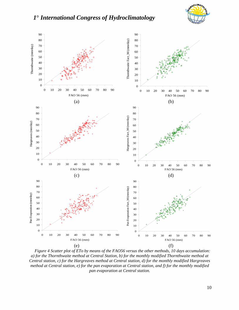
Figure 4c presents the scatter plot between the FAO56 and the Hargreaves-Samani methods at Central station, presenting a slight overestimation. However, in the Thornthwaite results (Figure 4a) a more severe underestimation is show. The pan Evaporation data finally presents great dispersion especially for daily evaluation; nevertheless for ten days accumulation it shows the same trend (Figure 4e).

This analysis reflects that the correction factor derived in the present case study depends on the station and the method. It is clearly not constant for the whole catchment.

From the above discussed figures, it might also be important to discuss the dispersion in the scatter plots of the Hargreaves method. When the Hargreaves method is compared with the FAO56 at Mairana station, regardless of the clear bias the dispersion is rather limited, which may indicate the suitable use of the Hargreaves method at this station. At Central station the dispersion is more noticed and the Viru Viru station presents the highest dispersion. This can directly be related to the importance of the aerodynamic factor at Viru Viru station when computing ETo. At Viru Viru station the average wind speed is almost 3 times that high as for Mairana station and still higher than the one at Central station.

Temesgen et al., (2005) found that higher wind speed combined with lower humidity results in lower values in the Hargreaves estimates. Lower wind speed combined with higher humidity results in higher values of the Hargreaves results. This is consistent with what has been found at


9

Mairana station: this station presents conditions of high humidity and low wind speed, and it shows overestimations by the Hargraeves method.

Other researchers have suggested possible overestimations of ETo by the Hargreaves method under humid environments and underestimations under windy conditions compared to the FAO56 method (Allen et al., 1998; Droogers and Allen, 2002; Temesgen et al., 1999). This agrees with the findings of the present case study at Viru Viru and Central stations.

At Central station, the Thornthwaite method underestimates ETo (Figure 5a), but with the annual correction factor it underestimates the lower ETo values whereas it overestimates the high values, Figure 5b. This problem is somehow solved with the monthly factor (Figure 5c).

In general it can be seen that the original Thornthwaite and Hargreaves methods under- or overestimate the daily ETo. After applying the annual correction factor these differences are somehow reduced. More significant improvement is, however, reached after applying a monthly correction factor to the prediction of the ETo using the temperature based methods (Figure 5b, 5d, 5f). The latter correction factor is therefore recommended in this study.

Figure 6 presents the evolution of the monthly correction factor for the Thornthwaite and Hargreaves methods. As was already noticed in the scatter ranked plot, the monthly correction factor is almost constant throughout the year at Mairana station, with a value near 0.8 for Hargreaves and 1.3 for Thornthwaite. At the Central station there is a slight variation of the factor, especially in the months of July and August, the windy months. However, these variations increase at the Viru Viru station, which has the higher wind speeds.


10

0

10

20

30

40

50

60

70

80

90

0 10 20 30 40 50 60 70 80 90

FAO 56 (mm)

Thor

nthw

aite

(mm

/day

)

0

10

20

30

40

50

60

70

80

90

0 10 20 30 40 50 60 70 80 90FAO 56 (mm)

Thor

nthw

aite

Fac

t_M

(mm

/day

)

(a) (b)

0

10

20

30

40

50

60

70

80

90

0 10 20 30 40 50 60 70 80 90

FAO 56 (mm)

Har

grea

ves (

mm

/day

)

0

10

20

30

40

50

60

70

80

90

0 10 20 30 40 50 60 70 80 90FAO 56 (mm)

Har

grea

ves F

act_

M (m

m/d

ay)

(c) (d)

0

10

20

30

40

50

60

70

80

90

0 10 20 30 40 50 60 70 80 90

FAO 56 (mm)

Pan

Evap

orat

ion

(mm

/day

)

0

10

20

30

40

50

60

70

80

90

0 10 20 30 40 50 60 70 80 90FAO 56 (mm)

Pan

Evap

orat

ion

Fact

_M (m

m/d

ay)

(e) (f) Figure 4 Scatter plot of ETo by means of the FAO56 versus the other methods, 10 days accumulation:

a) for the Thornthwaite method at Central Station, b) for the monthly modified Thornthwaite method at Central station, c) for the Hargreaves method at Central station, d) for the monthly modified Hargreaves method at Central station, e) for the pan evaporation at Central station, and f) for the monthly modified

pan evaporation at Central station.


11

0

1000

2000

3000

4000

5000

6000

7000

8000

9000

0 500 1000 1500 2000

Time (Days)

Cum

ulat

ive

ETo

(mm

)

FAO 56 AcuThornthwaite AcuThornthwaite Acu Fact_M

0

2

4

6

8

10

12

0 2 4 6 8 10 12FAO 56 (mm/day)

Mod

el (m

m/d

ay)

ThornthwaiteThornthwaite corr Fact_YThornthwaite corr Fact_M

(a) (b)

0

1000

2000

3000

4000

5000

6000

7000

8000

9000

0 500 1000 1500 2000Time (Days)

Cum

ulat

ive

ETo

(mm

)

FAO 56Thornthwaite AcuThornthwaite Acu Fact_M

0

2

4

6

8

10

12

0 2 4 6 8 10 12FAO 56 (mm/day)

Mod

el (m

m/d

ay)


(c) (d)

0

1000

2000

3000

4000

5000

6000

7000

0 500 1000 1500 2000Time (Days)

Cum

ulat

ive

ETo

(mm

)

FAO 56Thornthwaite AcuThornthwaite Acu Fact_M

0

1

2

3

4

5

6

7

8

9

0 1 2 3 4 5 6 7 8 9FAO 56 (mm/day)

Mod

el (m

m/d

ay)


(e) (f)

Figure 5. Cumulative and ranked scatter plots of ETo by means of the FAO56 method versus the other methods: a) for the Thornthwaite method at Central Station, b) for the corrected Thornthwaite method at

Central station, c) for the Thornthwaite method at Viru Viru station, d) for the modified Thornthwaite method at Viru Viru station, e) for the Thornthwaite method at Mairana station, and f) for the modified

Thornthwaite method at Mairana station


12

0.6

0.8

1

1.2

1.4

1.6

1.8Ja

n

Feb

Mar

Apr

May Jun

Jul

Aug Se

p

Oct

Nov Dec

Month

Coe

ffic

ient

Central _M Viru Viru_M Mairana_MCentral_Y Viru Viru_Y Mairana_Y

0.6

1

1.4

1.8

2.2

2.6

Jan

Feb

Mar

Apr

May Jun

Jul

Aug Se

p

Oct

Nov Dec

Month

Central _M Viru Viru_M Mairana_MCentral_Y Viru Viru_Y Mairana_Y

(a) (b) Figure 6. a) Evolution of the monthly correction factor for the a) Hargreaves method, and the

b) Thornthwaite method at the different stations

Table 3. Summary of the statistics and calibration coefficients found for the correspondence between the Thornthwaite and Hargreaves methods with the FAO56 method for the Piraí River Basin, Bolivia

Thornthwaite Hargreaves - Fact_Y Fact_M - Fact_Y Fact_M

RMSE* 1.352 1.373 1.249 1.026 0.898 0.856 Central ME* -0.614 -0.004 0.000 0.434 -0.002 0.000

RMSE* 1.864 1.803 1.588 1.248 1.130 0.965 Viru Viru ME* -0.990 0.033 0.000 -0.572 0.016 0.000

RMSE* 1.132 0.820 0.789 0.744 0.275 0.255 Mairana ME* -0.899 -0.007 0.000 0.659 -0.010 0.000

*in mm/day

Table 3 presents the basic statistics when comparing the temperature based methods (currently used in the region) against the FAO56 method, at the three CWS. The RMSE is reduced in all the cases after application of the correction factors. The ME for the monthly correction factor is zero given that the correction factors were based on minimization of the monthly bias.

Finally we can conclude that applying monthly correction factors to the temperature based methods can reach good quality results with an error in the order of less than 1 mm with respect to the FAO56 method. Therefore these factors can be applied in the TWS stations in order to obtain more realistic and accurate results.

FAO56 can handle missing climatic data, only Tmax and Tmin are required, therefore it is suggested to apply this method as standard. For further research, extra effort should be put in the data recompilation or digitalization since the mean air temperature should come from Tmax and Tmin measures.

A surprising bad result was observed for the pan evaporation measures, even with the use of monthly correction factors the improvements were almost imperceptibles. There are many factors that should be investigated (type of pan, installation of the pan, location of the pan,


13

environmental and climatic conditions, type of record). It is dangerous to use pan evaporation data in this conditions.

References

Alexandris, S., Kerkides, P., Liakatas, A., 2005. Daily reference evapotranspiration estimates by the ‘‘Copais’’

approach. Agric. Water Manage. 82, 371–386. Alfonsi, R., Pinto, H., Pedro, M., 1974. Estimativas das normais de temperaturas média mensal e anual do Estado de

Goiás (BR) em função de altitude e latitude. Caderno de Ciências da Terra, v.45, p.1-6. Allen, R.G., 1996. Assessing integrity of weather data for reference evapotranspiration estimation. Journal of

Irrigation and Drainage Engineering. ASCE 122 (2), 97–106. Allen, R.G., Pereira, L.S., Raes, D., Smith, M., 1998. Crop evapotranspiration: guidelines for computing crop water

requirements. FAO Irrigation and Drainage Paper no. 56, Rome, Italy. Amatya, D. M., Skaggs, R.W., and Gregory, J.D., 1995. Comparison of methods of estimating REF-ET. ASCE

Journal of Irrigation and Drainage Engineering 121 6, pp. 427–435. Cai, J., Liu, Y., Lei, T., Pereira, L.S., 2007. Estimating reference evapotranspiration with the FAO Penman–Monteith

equation using daily weather forecast messages. Agricultural and Forest Meteorology. Elsevier 145, 22–35. Cargnelutti, A., Tavares, J., Matzenauer, R., and Prestes, A., 2006. Altitude and geographic coordinates in the ten-

day mean minimum air temperature estimation in the State of Rio Grande do Sul, Brazil. Pesquisa Agropecuária Brasileira, vol.41, n.6, pp. 893-901. ISSN 0100-204X (in Portuguese).

Chiew, F.H.S., Kamaladasa, N.N., Malano, H.M., McMahon, T.A., 1995. Penman-Monteith, FAO-24 reference crop evapotranspiration and class-A pan data in Australia. Agricultural Water Management. Elsevier 28, 9–21.

Coelho, D., Sesiyama, G., Viera, M., 1973. Estimativa das temperaturas médias mensais e anual no Estado de Minas Gerais. Revista Ceres, v.20, p.455-459. (in Portuguese).

DehghaniSanij, H., Yamamotoa, T., Rasiah, V., 2004. Assessment of evapotranspiration estimation models for use in semi-arid environments. Agricultural Water Management. 64, 91–106.

Droogers, P., Allen, R.G., 2002. Estimating reference evapotranspiration under inaccurate data conditions. Irrigation and Drainage Systems 16, 33–45.

Feitoza, L., Scárdua, J., Sediyama, G., Valle, S., 1980. Estimativas das temperaturas médias das mínimas mensais e anual do Estado do Espírito Santo. Revista do Centro de Ciências Rurais, v.10, p.15-32. (in Portuguese).

Fritzsons, E., 2008. Relação entre Altitude e Temperatura: Uma Contribuição ao Zoneamento Climático no Estado do Paraná. Revista de Estudos Ambientais, V. 10, P. 40-48, 2008. (in Portuguese).

Harding, RJ, 1978. The variation of the altitudinal gradient of temperature in the British Isles. Geografiska Annaler. Series A, Physical Geography. 60, pp. 43–49. ISSN: 04353676 Blackwell Publishing

Garcia, M., Raes, D., Allen, R., and Herbas, C.: 2004, ‘Dynamics of reference evapotranspiration in the Bolivian highlands (Altiplano)’, Agricultural and Forest Meteorology 125(1–2), 67–82.

Gavilán, P., Lorite, I.J., Tornero, S., Berengena, J., 2006. Regional calibration of Hargreaves equation for estimating reference ET in a semiarid environment. Agric. Water Manage. 81, 257–281.

Hargreaves, G.H., Samani, Z.A., 1982. Estimating potential evapotranspiration. Journal of Irrigation and Drainage Engineering., ASCE 108 (3), 225–230.

Hargreaves, G.H. and Samani, Z.A. 1985. Reference Crop Evapotranspiration From Temperature. Applied Engineering in Agriculture. 1(2):96-99.

Jabloun, M., Sahli, A., 2008. Evaluation of FAO methodology for estimating reference evapotranspiration using limited climatic data – Application to Tunisia. Agric. Water Manage. 95, 707-715.

Jensen M.E. 1985. Personal communication, ASAE national conference, Chicago, IL. Lima, M., Ribeiro, V., 1998. Equações de estimativa da temperature do ar para o Estado do Piauí. Revista Brasileira

de Agrometeorologia, v.6, p.221-227. (in Portuguese). López-Urrea, R., Martın de Santa Olalla, F., Fabeiro, C., Moratalla, A., 2006. Testing evapotranspiration equations

using lysimeter observations in a semiarid climate. Agric. Water Manage. 85, 15–26. Martınez-Cob, A., Tejero-Juste, M., 2004. A wind-based qualitative calibration of the Hargreaves ETo estimation

equation in semiarid regions. Agric. Water Manage. 64, 251–264. Medeiros, S., Cecilio, R., Melo Júnior, J., Silva Junior, J., 2005. Estimativa e espacialização das temperaturas do ar

mínimas, médias e máximas na Região Nordeste do Brasil. Revista Brasileira de Engenharia Agrícola e Ambiental, v.9, p.247-255. (in Portuguese).


14

Meyer, S. J., Hubbard, K. G., and Wilhite, D. A. (1989). “Estimating potential evapotranspiration: The effect of random and systematic errors.” Agricultural and Forest Meteorology., 46, 285–296.

Pereira, A.R., Pruitt, W.O., 2004. Adaptation of the Thornthwaite scheme for estimating daily reference evapotranspiration. Agric. Water Manage. 66, 251–257.

Ponce, V. M., 1989; Engineering Hydrology, Principles and Practices; Prentice Hall, Englewood Cliffs, New Jersey. Pp 52.

Popova, Z., Kercheva, M., Pereira, L.S., 2006. Validation of the FAO methodology for computing ETo with missing climatic data application to South Bulgaria. Irrigation and Drainage - Wiley. 55, 201–215.

Sediyama, G., Melo Júnior, J., 1998. Modelos para estimateiva das temperaturas normais mensais médias, máximas, mínimas e anual no Estado de Minas Gerais. Engenharia na Agricultura, v.6, p.57-61. (in Portuguese).

Shamsudin, S., Hashim, N., 2002. Rainfall Runoff Simulation Using Mike11 NAM. Journal of Civil Engineering Vol. 15 No. 2.

Saxton, K. E. (1975). “Sensitivity analyses of the combination evapotranspiration equation.” Agricultural Meteorology., 15, (3) 343–353. Elsevier Science Ltd.

Temesgen, B., Allen, R. G., and Jensen, D. T. (1999). “Adjusting temperature parameters to reflect well-watered conditions.” J. Irrig. Drain. Eng., 125(1), 26–33.

Temesgen, B., Eching, S., Davidoff, B., and Frame, K., 2005, Comparison of some reference evapotranspiration equations for California, J. Irrig. Drain. Eng., ASCE 131 (2005) (1), pp. 73–84.

Thornthwaite, C.W., 1948. An Approach Toward a Rational Classification of Climate. Geographical Review. 38 (1):55-94.

Trajkovic, S., 2007. Hargreaves vs. Penman-Monteith under Humid Condition. J. Irrig. and Drain. Engrg., 133(1), 47-52.

Vanderlinden, K., Giraldez, J.V., Van Mervenne, M., 2004. Assessing reference evapotranspiration by the Hargreaves method in Southern Spain. J. Irrig. Drain. Eng. ASCE 129 (1), 53–63.

Wu, I. P., 1997. A Simple Evapotranspiration Model for Hawaii: The Hargreaves Model, CTAHR Fact Sheet, Engineer’s Notebook No. 106, College of Tropical Agriculture and Human Resources, University of Hawaii at Monoa.

international congress of hydroclimatologylhumss.fcyt.umss.edu.bo/archivos para...

Documents