INTERNATIONAL BENCHMARKING OF

NETWORK RAIL’S MAINTENANCE AND RENEWAL COSTS: AN

ECONOMETRIC STUDY BASED ON THE LICB DATASET (1996-2006)

Report for the Office of Rail Regulation

Andrew Smith

October 2008

2

Table of Contents EXECUTIVE SUMMARY ....................................................................................... 3

1. Introduction ........................................................................................................ 6

2. The LICB dataset ............................................................................................... 7

3. Potential efficiency measurement approaches ................................................ 10

4. Model specification and functional form........................................................... 14

4.1 Functional form........................................................................................... 14

4.2 LECG’s challenge to the Cobb-Douglas functional form............................ 15

4.3 Model specification..................................................................................... 17

5. Results for our preferred model ....................................................................... 19

5.1 An a priori justification for our preferred approach..................................... 19

5.2 LECG’s comments on the preferred model................................................ 20

5.3 Preferred model: key assumptions............................................................. 23

5.4 Preferred model: results (parameter estimates)......................................... 25

5.5 Preferred model: results (efficiency scores)............................................... 28

6. Results from alternative methods .................................................................... 30

6.1 General discussion of results across methods........................................... 31

6.2 The BC92 model put forward by LECG...................................................... 33

7. Sensitivity analysis........................................................................................... 35

8. ORR’s use of the econometric analysis in PR2008 ......................................... 37

9. Conclusions ..................................................................................................... 38

ANNEX 1: MAINTENANCE AND RENEWALS ONLY MODELS ........................ 41

A1.1 Maintenance-only models ........................................................................ 41

A1.2 Renewals -only models............................................................................ 42

REFERENCES .................................................................................................... 45

3

EXECUTIVE SUMMARY During 2007 and 2008, The Institute for Transport Studies (ITS), University of Leeds, undertook econometric work to inform ORR’s judgement on an appropriate efficiency target for the infrastructure manager over Control Period 4 (CP4). This work was conducted in conjunction with ORR and Network Rail, and culminated in a joint ITS / ORR report published in June 2008 (see ITS/ORR (2008)). Our interaction with Network Rail was mainly via Charles Robarts, David Rayner, Matthew Clements and David Smallbone, and their input was very useful in helping us develop our analysis over this period (though of course we recognise that Network Rail ultimately challenged the analysis). The work was peer reviewed by Dr Michael Pollitt from the Judge Business School, University of Cambridge. This work was used by ORR, alongside other evidence, in setting out its Periodic Review 2008 (PR2008) draft determination on efficiency published in June 2008. The data for the exercise was provided by the UIC (International Union of Railways). UIC has collected this dataset as part of its own Lasting Infrastructure Cost Benchmarking (LICB) exercise and kindly released this data to ORR and ITS for the purpose of informing PR2008 and also with a view to developing UIC’s own approach going forward. We have welcomed the interaction with Gerard Dalton and Teodor Gradinariu at UIC during the course of our work, and have found their input to be extremely useful in developing our analysis (though we note that in July 2008 UIC raised some concerns regarding the application of the econometric models within the context of PR2008). This paper sets out the results of the subsequent econometric work and its use as part of PR2008. It provides additional detail to support the summary report produced in June 2008 (see ITS/ORR (2008)). Since the econometric work was reviewed by LECG and Horton 4 Consulting over the summer of 2008, this report also refers to some of the points raised in those reports where relevant. The report should be read in conjunction with our response document to the challenges raised by LECG and Horton 4 Consulting (see Smith and Wheat (2008)). The key conclusions are set out below. In this report we have explained the model selection process and shown that the preferred econometric model is robust, both in its own right, and in the context of the vast array of other methods that we have applied to this dataset. Where relevant, we have referred to and refuted the challenges raised by LECG and Horton 4 Consulting during their work over the summer of 2008. For further details on the latter, see our response document (Smith and Wheat, 2008)). It should be noted that during our work some areas of analysis were outside the scope of ITS’s remit (for example, collating evidence on the extent to which companies were above or below steady-state). In these areas we took advice from ORR, and where this was done it is indicated in the relevant section of the report. We also comment, in general terms, on the way in which ORR used the econometric results in arriving at its draft efficiency determination. Our key findings are summarised below.

4

LECG’s assertion that a “fix” is required in order for the model to produce an estimate is shown to be incorrect. Furthermore, we have shown that the method used to derive the variance co-variance matrix (from which the standard errors and hence the means of determining the precision of the estimates are derived) is an accepted and widely used approach, and that alternative testing procedures also provide support for the method used. The preferred model also produces plausible estimates for the model parameters, which are also statistically significant at the usual levels of significance1. It also produces a plausible time path of efficiency for Network Rail over the period: that is, improving after privatisation2, deteriorating after Hatfield, before improving during CP3. As noted, our preferred model also produces similar efficiency estimates for Network Rail to those from the other methods that we have tested, and there is also strong conformity of efficiency rankings (for all firms) across the different methods applied. LECG’s assertion that the Cobb-Douglas functional form adopted in our study violates economic theory in the multiple output case is shown to be incorrect (see Smith and Wheat (2008). LECG’s assertion is based on a single quote from one textbook, which has been taken out of the context of the wider theoretical and empirical literature, and indeed even the book from which the quote is taken. It is clear from the literature that the multiple output Cobb-Douglas cost function does not violate any required theoretical property of a cost function in a regulated industry, such as railways, where output levels are typically assumed to be exogenously determined (see, for example, Klein (1953), Nerlove (1965), and Coelli and Perelman (2000)). Indeed, in Smith and Wheat (2008) we show that this functional form is widely used in both academic and regulatory studies. The appropriate functional form is, instead, an issue for econometric testing and, as noted in the ITS/ORR June 2008 report, we have tested the Cobb-Douglas model and found it to be preferred to the alternatives. Furthermore, LECG have themselves utilised a multiple-output Cobb-Douglas cost function in their recent (2005) study of postal delivery office efficiency, so it extremely puzzling that they have raised this issue in criticism of our work. This functional form has also been used by OFWAT, as LECG note in their 2005 study. In all of the other areas of concern raised by the consultants – which include data quality, possible omitted variables, and the modelling of railways out of steady-state, these have either been directly addressed in the modelling approach, or

1 As demonstrated by the standard errors derived from the variance co-variance matrix, and alternative testing procedures as noted.

2 Of course, the low costs experienced during the Railtrack period may have been indicative of inadequate work being carried out, rather than efficient operation. This issue is addressed via the steady-state adjustment carried out prior to estimation discussed below.

5

ORR has done other work to verify the appropriateness of the approach taken (it was recognised that that further work with regard to omitted variables and quantifying the extent to which railways are out of steady-state was outside ITS’s remit, and in these areas we took advice from ORR). Ultimately, there are strong reasons for using the preferred model (in its own right) as the starting point for ORR’s analysis, based on its statistical and other properties. The preferred model also produces an efficiency gap in the middle of the range of estimates resulting from the various models estimated and sensitivity analysis conducted. Furthermore, ORR benchmarks Network Rail against the upper quartiles, and not the frontier, which is a conservative approach given that the preferred model is a stochastic frontier model. In our view, ORR’s starting point for its efficiency determination is therefore a reasonable one, based on the econometric work carried out. The econometric results are also supported by the regional international econometric study (see ITS/ORR (2008)). From the starting point of a 37% efficiency gap, ORR then makes a further discounting assumption that two thirds of the gap can be closed over CP4. Furthermore, ORR has combined the results of the econometric work with other evidence in arriving at its draft efficiency determination. We therefore consider that, in general terms, ORR has made appropriate use of the econometric work in its analysis, although ITS did not review the other evidence commissioned / produced by ORR, and was not involved in the details of the process by which ORR reached its draft efficiency determination. This process resulted in the efficiency gap from the preferred econometric model of 37% being scaled down to an efficiency target for maintenance and renewals in CP3 of 22% (see ORR (2008)3) and, of course, required ORR to exercise its regulatory judgement.

3 See page 141.

6

1. INTRODUCTION During 2007 and 2008, The Institute for Transport Studies (ITS), University of Leeds, undertook econometric work to inform ORR’s judgement on an appropriate efficiency target for the infrastructure manager over Control Period 4 (CP4). This work was conducted in conjunction with ORR and Network Rail, and culminated in a joint ITS / ORR report published in June 2008 (see ITS/ORR (2008)). Our interaction with Network Rail was mainly via Charles Robarts, David Rayner, Matthew Clements and David Smallbone, and their input was very useful in helping us develop our analysis over this period (though of course we recognise that Network Rail ultimately challenged the analysis). The work was peer reviewed by Dr Michael Pollitt from the Judge Business School, University of Cambridge. This work was used by ORR, alongside other evidence, in setting out its Periodic Review 2008 (PR2008) draft determination on efficiency published in June 2008. The data for the exercise was provided by the UIC (International Union of Railways). UIC has collected this dataset as part of its own Lasting Infrastructure Cost Benchmarking (LICB) exercise and kindly released this data to ORR and ITS for the purpose of informing PR2008 and also with a view to developing UIC’s own approach going forward. We have welcomed the interaction with Gerard Dalton and Teodor Gradinariu at UIC during the course of our work, and have found their input to be extremely useful in developing our analysis (though we note that in July 2008 UIC raised some concerns regarding the application of the econometric models within the context of PR2008). This paper sets out the results of the subsequent econometric work, the model selection procedure, and its use as part of PR2008. It provides additional detail to support the summary report produced in June 2008 (see ITS/ORR (2008)). Since the econometric work was reviewed by LECG and Horton 4 Consulting over the summer of 2008, this report also refers to some of the points raised in those reports where relevant. The report should be read in conjunction with our response document to the challenges raised by LECG and Horton 4 Consulting (see Smith and Wheat (2008)). It should be noted that during our work some areas of analysis were outside the scope of ITS’s remit (for example, collating evidence on the extent to which companies were above or below steady-state). In these areas we took advice from ORR, and where this was done it is indicated in the relevant section of the report. We also comment, in general terms, on the way in which ORR used the econometric results in arriving at its draft efficiency determination. The remainder of the paper is structured as follows. Section 2 describes the LICB dataset. Section 3 discusses the range of possible efficiency methodologies that might be used and which method, a priori, might be preferred in the present context. Section 4 discusses model specification and the functional form adopted. Section 5 then presents the results of our preferred model, and the results of the other efficiency methods that we have applied to the data are presented in section 6. Section 7 presents the results of the sensitivity analysis that was

7

carried out. Section 8 discusses the use of the econometric results as part of PR2008. Section 9 concludes.

2. THE LICB DATASET As part of its own benchmarking analysis, and in particular the LICB work, the UIC has developed a potentially very useful dataset. It consists of data for 13 infrastructure companies (or infrastructure divisions within integrated companies) over a period of eleven years. We have reason to be relatively confident in the consistency of the LICB data, given the efforts made to standardise definitions, although we note comments from Network Rail that there are likely to be some limitations in terms of consistency as with any dataset of this nature. UIC uses this dataset in its approach to international benchmark (see UIC (2007) and Smith and Wheat (2008) for further details). The availability of multiple years on the same companies is also highly advantageous, as it avoids the danger of focusing on a single year snap-shot which might be impacted by year-to-year fluctuations in expenditure (particularly in respect of renewals). Furthermore, the dataset contains a wide range of variables in addition to the key measures of track length and traffic volumes.

Table 1: List of LICB study countries

Country Company

UK Network Rail Netherlands ProRail Norway Jernbaneverket Portugal Refer Finland RHK Sweden Banverket Ireland Irish Railways Belgium Infrabel Germany DB Austria OBB Italy FS (RFI) Denmark BDK Switzerland SBB Below we briefly describe the key variables from the LICB dataset that we have used in our analysis and any changes made to the raw data provided by UIC. The raw data provided by UIC contained in excess of thirty variables. The variables that were ultimately included in our analysis are listed below. These were the variables for which there was sufficient coverage of the data across the different companies and years.

8

• Cost Data

o Maintenance costs o Total costs (Maintenance + renewals)

• Network Size

o Track kilometres o Route kilometres o Single track kilometres o Electrified track kilometres

• Final Outputs

o Passenger train kilometres o Passenger tonne kilometres o Total tonne kilometres o Freight train kilometres o Freight tonne kilometres o Total train kilometres

• Network Characteristics

o Ratio of single track to route kilometres (as a measure of the extent

of single / multiple track) o Proportion of track electrified o Number of stations per route km o Number of switches per track km

Whilst the above list includes a wide range of potential cost drivers, ideally we would have wanted to include “quality” measures (e.g. track geometry), as well as asset age. We would also be interesting in exploring the impact of different safety standards and possessions regimes on cost. However data is not currently available although we hope that if UIC and ORR want to take this work forward in the future that we might be able to include such measures for a future round of the analysis if the data can be collected. Further work in this area during PR2008 was outside ITS’s remit. However, as discussed in section 5, following work carried out by ORR, an adjustment is made to Network Rail’s costs to address the possibility that Network Rail is currently renewing at above steady-state levels, and ORR (and Network Rail) have also undertaken parallel analysis to assess the impact of other possible omitted variables on our analysis. The dataset was taken largely as given, although some analysis was done to check for very large, discrete swings in data values from year to year. We determined whether these swings were justified by changes in other variables

9

correlated to the trend examined and whether the trend appeared to be confirmed by other published sources or data collected. As a result of this analysis a small number of data points were changed where the evidence strongly suggested that an input error had been made4. In addition, we also made a small number of changes to the data set where gaps existed in the dataset (e.g. where data for a variable for a particular company was missing for a single year). Two methodologies for infilling were applied as follows:

(a) For variables for which there were other related variables, with which we would reasonably expect the variable to be correlated, we used the relevant annual growth rate of the related variable to pro-rata the missing observations. This applied to the traffic variables in particular; and

(b) For the physical variables and cost variables for which no clearly correlated variables were available, we used simple interpolation / extrapolation to obtain the relevant observation from the overall trend in that variable.

We expect the impact of this infilling to be relatively small given that we have adopted a reasonable approach – that is, the variables in question do tend to change steadily over time - and also because the number of data points that we have filled in is relatively small. On inspection the data relating to network size, single track, electrification variables and passenger and freight train-km appeared to be well behaved. However we note that the passenger and freight tonnage data appeared to be more volatile, and we also had some concerns over the data on switches and stations. As shown in section 5, however, none of these latter variables were included in the preferred model specification (as they were found not to be statistically significant and because we had concerns over the quality of the data for those variables). Finally, cost data were supplied in both local currency and Purchasing Power Parity (PPP) Euros. So that we could be sure of the underlying assumptions concerning inflation and the PPP adjustment, we started with the local currency information and used Purchasing Power Parity (PPP) exchange rate data from the OECD to convert the data to a common currency and price level for each year. In this way, differences in national price levels which affect costs were controlled for. To control for inflation, the data was then deflated to a common year price level (with German Euros in 2006 as the numeraire). These real costs were then the final figures used in our analysis5. We did not have sufficient information to separately include a wage rate variable in the model, although general (economy wide) wage rate differences will be

4 See ORR internal documentation (Powerdocs #277320). Most of the changes were

made to variables that were not subsequently included in the preferred model. 5 See ORR internal documentation (Powerdocs #277315).

10

accounted for via the PPP adjustment. However, ORR advised us that there was insufficient evidence to judge whether Network Rail faced higher relative (rail specific) wage rates than in other countries (or at least that if differences did occur, wages might be thought of as partially endogenously determined and thus under Network Rail’s control). We understand that over the summer of 2008 ORR carried out further work on this question using available data which supports the original analysis. In respect of taking this work forward beyond PR2008, we would expect to revisit the data to see whether any of the infilled data can be replaced with actual data, to discuss any other possible limitations of the dataset, and to investigate the availability of data on other key cost drivers.

3. POTENTIAL EFFICIENCY MEASUREMENT APPROACHES In this paper we apply econometric methods6 to relate maintenance and renewals costs to the relevant cost drivers included in the LICB database. These methods allow us to test the extent to which costs can be explained by the relevant cost drivers and, once those relationships have been estimated, to use that information to estimate the relative efficiency of a company compared to other companies in the dataset. Of course, we recognise that the LICB data is limited in terms of the number of cost drivers, and ideally additional variables would be included in the model. We therefore accept that there is some uncertainty here, and that the distance from the frontier may reflect both inefficiency and the impact of omitted variables. However, we have taken advice from ORR in this regard (further work in this respect being outside ITS’s remit) and ORR, having looked at the evidence, has concluded that there is no reason to believe that incorporating additional variables would necessarily lead to a significant change in the model results and be favourable to Network Rail, since there will be factors which disadvantage Network Rail as well as benefiting it. In addition, as discussed in section 5 below, a “steady-state” adjustment has been made to Network Rail’s costs whilst the leading firms are assumed to be

6 During some preliminary analysis, based on the dataset for the years 1996-2005, we also

applied the linear programming method, data envelopment analysis (DEA) to the data and this produced similar results to the COLs econometric results. For the latter reason, and also because of the difficulty of dealing with scale and density effects in a DEA framework, without resorting in any case to a two stage approach that involves econometric estimation in the second stage, we did not apply the DEA method to the final 1996-2006 dataset.

11

broadly in steady-state. We also understand that during the summer of 2008 ORR has undertaken some further analysis based on the available data on relative renewal levels for some of the countries in the UIC’s LICB dataset which supports the original analysis. We therefore consider that appropriate supporting work has been done in parallel to the econometric study to address the concerns raised. Furthermore, as discussed in section 8 of this report, ORR has applied discount factors to the raw results of the econometric models to reduce the level of savings required during CP4 (by aiming off the frontier, and requiring two thirds of the gap to be delivered over CP4), and also combined the results with other evidence. We therefore consider that ORR has made appropriate use of the econometric study in reaching its draft determination, although ITS did not review the other evidence commissioned / produced by ORR, and of course the efficiency determination process requires ORR to exercise its regulatory judgement. Given these factors, in the remainder of the report we interpret the final results from the econometric work as efficiency scores. There are a range of econometric methods that might be applied in the present context. Our preferred model has the following error structure:

ititit uv +=ε (1) where the i and t subscripts refer to the firms in the sample and time respectively. The ( itv ) term is a random, stochastic, component representing unobservable factors that affect the firm’s operating environment (often referred to as random noise). This term is distributed symmetrically around zero. A further one sided error term is then added to capture inefficiency ( itu ), where the inefficiency term in turn has the following time varying structure (and is based on the model proposed by Cuesta (2000)):

)t(guu iit ⋅= ))(exp()( tTtg i −⋅= η T,,1t Κ= (2)

where the iη are a set of firm specific parameters to be estimated, and iu has a one sided normal distribution with zero mean and variance 2

uσ . If iη is positive for an individual firm, this indicates that efficiency is improving for that firm over time, and vice versa for a negative iη . This model therefore captures a number of important and desirable features for efficiency estimation. First of all, it is one of a class of models, referred to as stochastic frontier models, that distinguishes between random noise and inefficiency, and therefore is not overly influenced by outliers. Second, it allows efficiency to vary over time and in flexible manner, so that a time varying efficiency parameter is estimated for each firm, so that the direction and extent of efficiency variation over time can be different for each firm. Third, the variation in efficiency over time is nevertheless structured, and not random - and the model

12

thus recognises the panel structure in the data (that is, we have a dataset of thirteen firms over 11 years, and not simply a dataset of 143 firms7). Furthermore, our preferred model incorporates additional flexibility in respect of the time path of efficiency for Network Rail. First, we have split the sample, such that the observations for Britain are treated as two firms, one for the pre-Hatfield period (1996 to 1999 inclusive), and one for the post-Hatfield period (2000-2006); though we note that the models with and without this separation produce very similar results. Second, we have incorporated an additional squared term into equation (2) for Network Rail which allows the model to (potentially) pick up a turning point in inefficiency during the post-Hatfield period8. This was considered important by ORR, given the expectation that efficiency deteriorated during the early post-Hatfield years, before improving as the CP3 efficiency savings start to have an impact. In general, incorporating additional flexibility into the efficiency time path for Network Rail seems desirable given the substantial changes in costs that have occurred over the period under analysis. In the analysis that follows, the preferred model is referred to as the flexible Cuesta00 model. As described in section 6 we have also applied a wide range of other efficiency measurement approaches in order to validate our preferred model. Some of these models are “nested” within our preferred models (as simpler versions of it), and the preferred model can therefore be tested against these nested alternatives. So, if we do not include the additional squared term, the model becomes a straightforward application of Cuesta (2000); and this model is therefore referred to as the simple Cuesta00 model in the results that follow. Likewise, the Battese and Coelli (1992) time varying efficiency model is a further simplification that assumes a common η parameter for all firms, so that all firms are forced (by assumption) to have the same direction of efficiency change over time; an assumption that could be particularly restrictive in the present context, where not all firms in the sample might be assumed to have followed a similar profile of efficiency change as Network Rail. Finally, our preferred model nests the time invariant stochastic frontier model proposed by Pitt and Lee (1981). This model assumes efficiency to be invariant for all firms over time, which could be considered restrictive, although it has the advantage of simplicity in that it produces a single efficiency score for each firm. However, as noted above, we do enable some efficiency variation for Network Rail in this model by splitting the British data into two firms (pre- and post-Hatfield).

7 As implied by some models which pool the data and treat each observation (11x13=143) as a separate firm.

8 The inefficiency specification in the preferred model is an extension of Cuesta (2000) and can also be seen as a specific case of the general model outlined in Orea and Kumbhakar (2004)).

13

In addition to the Pitt and Lee (1981) model, which is a random effects, maximum likelihood model, we also estimate the more traditional fixed effects and random effects (the latter estimated by generalised least squares) models (see Schmidt and Sickles (1984)). These are again time invariant models, but they do not require an assumption to be made about the distribution of the inefficiency term. Other models that we have considered include two commonly estimated, simple, pooled models, the corrected ordinary least squares (COLS) and the pooled stochastic frontier model. Both models do not recognise the panel structure of the data, and treat each observation (across firms, and over time) as a separate firm. This is, of course, an unrealistic assumption9, but these models are often estimated and we include them for completeness10. However, a key point is that we have used a combination of several techniques to help us try and develop the most robust models possible, and to provide us with a range of estimates using different techniques, as a “cross check”. Cross checking the results of benchmarking analysis of this sort in economic regulation by using alternative techniques is now considered regulatory best practice. There are also various test statistics that can help us in choosing our preferred models. Further details regarding the choice of methods are provided in sections 5-8. It should also be noted that all of these methods have been used in the academic literature therefore providing a precedent. In a regulatory context, the COLS method has been used in other UK regulated industries (for example by OFGEM, OFWAT and OFTEL/OFCOM)) at least in a cross-sectional context and stochastic frontier analysis has also been used (e.g. OFTEL/OFCOM). UK academics and water companies have applied panel data techniques to estimate

9 It should also be noted that these models allow efficiency to vary over time in a very flexible way. However, this variation is, ultimately random, which is a major problem in terms of interpretation in a regulatory context.

10 We have also considered models that allow efficiency to be decomposed into a persistent and time varying component (see Kumbhakar and Hjalmarsson (1995) and Kumbhakar and Heshmati (1995)). The main drawback of these models is that, as with the simple pooled models, the time varying component is assumed to vary randomly over time, which is a problem for testing the temporal variation in efficiency. These models have more recently been re-interpreted in an unobserved heterogeneity context, with the time invariant inefficiency term assumed to be unobserved heterogeneity, and the (random) time varying component to be inefficiency (the so-called “true” models; see Greene (2005)). However, this interpretation suffers from the problem that some inefficiency is likely to be persistent and, as noted above, that the time varying element is assumed to be random over time. We note that the “true” random effects model produces an error message on estimation, and the “true” fixed effects model produces identical results to the fixed effects model. For this reason, and also because these models are relatively new and their interpretation unclear, they are not discussed further.

14

relative efficiency in the water industry, and OFWAT is currently considering modifying its approach to efficiency analysis to include panel techniques.11 In the light of the above we might not necessarily want to reject any of the individual approaches unless there are very strong reasons for doing so in our particular case, although we may want to indicate our preferred model or models. As is common in studies of this nature we will also want to look at the extent of conformity in the results of different approaches, both in terms of the absolute efficiency scores and the relative rankings. All of the models have been estimated using the econometric software LIMDEP version 9. 4. MODEL SPECIFICATION AND FUNCTIONAL FORM In this section we discuss the functional form adopted in our study, the challenge to that functional form by LECG (in their September 2008 report), and the model specification adopted in terms of the variables included in the model.

4.1 Functional form In our analysis we have estimated a number of different functional forms:

• the linear form: all variables enter the cost function without any transformation;

• the log-linear or Cobb Douglas form: as for the linear function but with the dependent and explanatory variables entered in natural logarithms; and

• Translog: as for the Cobb Douglas but with square and cross terms for the main traffic and scale variables.

We have tested these forms against each other. In the case of the Cobb-Douglas versus the translog, the former is nested within the latter, so these two forms can be tested via a set of appropriate linear restrictions. We test between the linear and log-liner form via the Box Cox Test proposed by Zarembka (1968). Details of this test can be found in Dougherty (1992). This test transforms the dependent variables in such away that the fits of the models can be compared and then a test can be conducted to determine whether one is statistically better than the other12. In addition to statistical testing, we also looked at the reasonableness of the resulting parameter estimates. As reported in section 5 below, based on all of the above analysis, the Cobb-Douglas form is found to be the preferred functional form over both the linear and translog alternatives.

11 See for example Review of the Approach to Efficiency Assessment in the Regulation of

the UK Water Industry http://www.ukwir.org/ukwirlibrary/91524 12 Note that this test uses the residual sum of squares so we considered the ordinary least

squares (OLS) model only.

15

4.2 LECG’s challenge to the Cobb-Douglas functional form At this point we note that in their September (2008) report LECG have challenged the use of the Cobb-Douglas functional form from an economic theory perspective. This challenge is specifically addressed in Wheat and Smith (2008), and the discussion there is repeated below. In particular, LECG note the following:

“A great virtue of the Cobb-Douglas functional form is that its simplicity enables us to focus our attention where it belongs, on the error term, which contains information on the cost of inefficiency. As an empirical matter, however, the simplicity of the Cobb-Douglas functional form creates two problems. As Hasenkamp (1976) noted long ago, in a commentary on Klein’s (1947) famous railroad study, a function (or frontier) having the Cobb-Douglas form cannot accommodate multiple outputs without violating the requisite curvature properties in output space”; see LECG (2008), page 11, taken from Kumbhakar and Lovell (2000), page 143.

LECG then question why ITS/ORR “have selected a functional form that is incompatible with economic theory”, without giving any further explanation as to what they perceive the problem to be. In response we make three points. First, LECG have taken this quote out of the context of the wider theoretical and empirical literature, and indeed even the book from which the quote is taken. The multiple output Cobb-Douglas cost function does not violate any required theoretical property of a cost function in a regulated industry, as further reading of the earlier sections of the same textbook from which LECG derive the above quote demonstrates13. The problem applies only for profit maximising firms in a purely competitive industry (where firms can choose output levels to maximise profits), since the conditions for profit maximisation are violated. It does not apply in a regulated industry such as railways, where railway output levels are typically assumed to be exogenously determined. This point is clearly made in Klein (1953):

“This same problem does not arise in a model of a regulated industry….”; see Klein (1953), page 227.

13 See Kumbhakar and Lovell (2000), pages 20 and 34. See also Coelli, Rao, O’Donnell and

Battese (2005), page 23.

16

Coelli and Perelman (2000) also quote Klein (1953) and make a similar point14. The distinction between the perfectly competitive and regulated case is also made by Nerlove (1965) – this source being referenced in the Hasenkamp (1976) paper referred to in the paragraph quoted by LECG above. Nerlove (1965) dedicates a whole chapter to discussing Klein’s work, and notes the following:

“The study is especially interesting for the techniques employed; and while these are primarily applicable only in the case of a regulated industry [emphasis added], several lessons may be drawn of more general interest”; see Nerlove (1965), page 61.

Secondly, the error in LECG’s interpretation of the quote in their report is made clear by the fact that multiple output cost functions have been estimated in the literature in numerous cases – either in their own right, or as part of a statistical testing approach alongside other functional forms15. Some key regulatory studies have also adopted this approach, for example the recent and highly regarded study commissioned by the German Network Agency in respect of gas and electricity distribution benchmarking in Germany (see Sumicsid (2007))16. Indeed, a well acknowledged practical advantage of the Cobb-Douglas function, over the translog form, is its parsimony17. Thus the functional form for the cost function is in fact an issue for econometric testing, rather than being a required theoretical property. As noted in our June report we have tested the Cobb-Douglas model and found it to be preferred to the other alternatives (e.g. linear and translog).

14 Coelli and Perelman (2000), page 1969. 15 The following are just a few examples: Farsi and Filippini (2006), Barros (2005), Mulatu

and Crafts (2005) and Eeckaut, Tulkens and Jamar (1993). 16 For example, pages 35-38. 17 Coelli, Rao, O’Donnell and Battese (2005), page 212.

17

Finally, LECG themselves estimate a multiple output cost function in their work on postal cost efficiency (see LECG (2005)). For example, in their analysis of postal delivery office costs they estimate a Cobb-Douglas cost function:

“Another common functional form is the Cobb-Douglas form…We tested a number of alternative functional forms and found that the Cobb-Douglas form provided the best empirical fit to the data”; see LECG (2005), page 351.

and list the following variables as “measures of scale and output”:

“...measures of scale and output include: number of delivery points; percentage of delivery points that are business; and weighted and disaggregated volumes”; see LECG (2005), page 342.

In their 2005 study, LECG also list more than a dozen additional variables that may be thought of as output or output characteristic variables (for example, volume of mail redirected and length of road per delivery point)18 for possible inclusion in the model. They also note the OFWAT use the Cobb-Douglas form in their analysis19. We therefore question why LECG consider our approach to be incompatible with economic theory, as it would imply that the approach they have adopted elsewhere suffers from the same problem.

4.3 Model specification Having selected an appropriate functional form, the next step is to decide the dependent variables (cost measures) and independent variables (cost drivers) to include in the model. The models that we have estimated (and reported in our

18 See pages 343-344. The full list of variables included in the delivery office Cobb-Douglas

cost function model are as follows: volume per delivery point, number of delivery points, length of road per delivery point, percentage of business delivery points, mail re-direction, average wage rate, wage competitiveness index, major city centre dummy, urban dummy, sub-urban dummy, rural dummy, number of RM2000 frames – see page 352. Of course, the precise definition of what is an output, as opposed to being an output characteristics is often open to debate, but it is clear that the variables listed above are similar in nature to the inclusion of route length and passenger and freight density in our preferred model.

19 See page LECG (2005), page 351. It is clear that some of the OFWAT models include more than one output variable.

18

June (2008) Powerpoint report) are listed below in Table 2. The preferred model, with its two alternative specifications (with and without the steady-state adjustment), is shown in the first two columns (with shading).

Table 2: Model specifications

Dependent variable TOTSS TOTAL MAIN RENEWSS RENEW CONST

CONST

CONST

CONST

CONST

ROUTE ROUTE ROUTE ROUTE ROUTE PASSDR PASSDR PASSDR PASSDR PASSDR FRDR FRDR FRDR FRDR FRDR SING SING SING SING SING ELEC ELEC ELEC ELEC ELEC SWITCH SWITCH TIME TIME TIME TIME TIME

Cost drivers20

TIME^2 TIME^2 TIME^2 TIME^2 TIME^2 The definitions of the variables names in Table 2 are as follows:

• TOTSS2 = Ln (maintenance + renewal costs) where the renewal costs have been subject to a steady-state adjustment (see section 5 below)21;

• TOTAL = Ln (maintenance + renewal costs), based on the raw renewal costs;

• MAIN = Ln (maintenance); • RENEWSS = Ln (renewal costs) where the renewal costs have been

subject to a steady-state adjustment (see section 5 below); • RENEW = Ln (renewal costs), based on the raw renewal costs; • ROUTE = Ln (route-km); • PASSDR = ln (passenger train density)22; • FRDR = Ln (freight train density) • SING = Ln (single track-km divided by route-km); • ELEC = Ln (electrified track-km divided by track-km); • SWITCH = Ln(number of switches per track km); • TIME = time trend; • TIME = time trend squared.

For the single track and electrification variables we also ran the total cost (with steady-state) specification with these variables as proportions (not logged). Across all of the different efficiency models estimated (discussed in section 3

20 As is standard, the cost drivers are normalised by the sample mean prior to estimation to

permit straightforward interpretation of the parameters in the more flexible translog models.

21 All costs are expressed in PPP Euros 2006 prices 22 That is, Ln (passenger train-km/route-km).

19

above, and shown in sections 5 to 8 below) the efficiency score for Network Rail in 2006 was either very close to or lower than the equivalent models with the variables in log form23. Furthermore, the efficiency score (all firms) correlation coefficient between the two alternatives for the preferred total cost model (with steady-state adjustment) is very high (0.96), indicating that these models are producing very similar results. The log form model was retained because the parameter estimates on the key traffic and scale variables were more plausible and statistically significant than in the alternative case24. In addition, we have tested the inclusion of further variables, as well as alternative specifications, for example where the impact of traffic volume is handled via a single measure (total train-km density or total tonne-km density). These sensitivities are reported in section 7 below. It is shown that these sensitivities support the results of the preferred model.

5. RESULTS FOR OUR PREFERRED MODEL This section sets out our results for the preferred model. It starts with a reminder of the reasons, a priori, for supposing that this model is appropriate in the present context for estimating Network Rail’s efficiency performance versus the other countries in the sample. Then, since LECG have challenged the technical aspects of this model, we deal with their comments, before discussing the results and the reasons (based on statistical and other considerations) why this we selected this model as our preferred approach.

5.1 An a priori justification for our preferred approach As noted in section 3 above, our preferred approach has a number of important and desirable features for efficiency estimation. First of all, it distinguishes between random noise and inefficiency, and therefore is not overly influenced by outliers. Second, it allows efficiency to vary over time and in flexible manner, so that a time varying efficiency parameter is estimated for each firm. The direction and extent of efficiency variation over time can therefore be different for each firm. Third, the variation in efficiency over time is nevertheless structured, and not random. Furthermore, our preferred model incorporates additional flexibility in respect of the time path of efficiency for Network Rail. First, we have split the sample, such

23 For the preferred total cost (with steady-state adjustment) model, Network Rail’s efficiency

score for 2006 is 0.59 as compared with 0.60 when the variables are expressed in log form.

24 Since the efficiency scores are so highly correlated between the models, it appears that the parameter estimates are, overall, explaining the variation in cost in a similar way.

20

that the observations for Britain are treated as two firms, one for the pre-Hatfield period (1996 to 1999 inclusive), and one for the post-Hatfield period (2000-2006)25. Second, we have incorporated an additional squared term into equation (2) for Network Rail which allows the model to (potentially) pick up a turning point in inefficiency during the post-Hatfield period26. This additional flexibility was considered important by ORR, given the expectation that efficiency deteriorated during the early post-Hatfield years, before improving as the CP3 efficiency savings start to have an impact. In general, incorporating additional flexibility into the efficiency time path for Network Rail seems desirable given the substantial changes in costs that have occurred over the period under analysis. In the analysis that follows, the preferred model is referred to as the flexible Cuesta00 model.

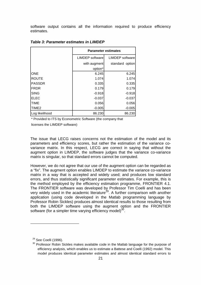
5.2 LECG’s comments on the preferred model LECG refers to a technical problem with our preferred model and the supposed fix that we have employed to make the model work. In this section we first respond to this point and show that the “fix” is in fact an accepted and very widely used approach to estimating the variance co-variance matrix for stochastic frontier models. We go on to argue why we think the model is robust (on its own terms). In sections 6 to 8 we also show that the preferred model is supported by the results of the vast array of other methods that we have applied to this dataset. This is not correct. The so called “fix” that we have used is an augment option to the standard stochastic frontier command which was provided to ITS by Econometric Software, the company that licenses the LIMDEP 9 software (in relation to an efficiency analysis conducted on a different data set for an unrelated project during 2007; and which is explained further below). When the model is run using the standard option (so without the augment option (as LECG has done)), LIMDEP gives the message “normal exit from iterations”, which indicates that the model has estimated. It is then a matter of requesting LIMDEP to produce the output from that estimation27. As will be seen from Table 3 below, the parameter estimates are identical to those obtained when using the augment option28. It is clear from Table 3 that these models are identical; and the

25 Though we note that the models with and without this separation produce very similar

results. 26 As noted earlier, the inefficiency specification in the preferred model is an extension of

Cuesta (2000) and can also be seen as a specific case of the general model outlined in Orea and Kumbhakar (2004)).

27 This involves the addition of the standard “OUTPUT=3” term to the LIMDEP code. The resulting output also confirms that the model has converged.

28 The parameters relating to efficiency change for each firm are also the same but are omitted for brevity.

21

software output contains all the information required to produce efficiency estimates.

Table 3: Parameter estimates in LIMDEP

LIMDEP software LIMDEP software

with augment standard optionoption*

ONE 6.245 6.245ROUTE 1.074 1.074PASSDR 0.335 0.335FRDR 0.179 0.179SING -0.918 -0.918ELEC -0.037 -0.037TIME 0.056 0.056TIME2 -0.005 -0.005Log likelihood 86.230 86.230

* Provided to ITS by Econometric Software (the company that

licenses the LIMDEP software)

Parameter estimates

The issue that LECG raises concerns not the estimation of the model and its parameters and efficiency scores, but rather the estimation of the variance co-variance matrix. In this respect, LECG are correct in saying that without the augment option in LIMDEP, the software judges that the variance co-variance matrix is singular, so that standard errors cannot be computed. However, we do not agree that our use of the augment option can be regarded as a “fix”. The augment option enables LIMDEP to estimate the variance co-variance matrix in a way that is accepted and widely used; and produces low standard errors, and thus statistically significant parameter estimates. For example, this is the method employed by the efficiency estimation programme, FRONTIER 4.1. The FRONTIER software was developed by Professor Tim Coelli and has been very widely used in the academic literature29. A further comparison with another application (using code developed in the Matlab programming language by Professor Robin Sickles) produces almost identical results to those resulting from both the LIMDEP software using the augment option and the FRONTIER software (for a simpler time varying efficiency model)30.

29 See Coelli (1996). 30 Professor Robin Sickles makes available code in the Matlab language for the purpose of

efficiency analysis, which enables us to estimate a Battese and Coelli (1992) model. This model produces identical parameter estimates and almost identical standard errors to

22

It should be noted that both approaches to estimating the variance co-variance matrix (that is, with and without the augment option) are accepted approaches. However, in the present context, one method implies that the parameters of the model are not estimated precisely, whilst the other suggests (with the augment option) that we can obtain quite precise estimates. Further comment is therefore warranted. We are confident in the results from our preferred model for the following reasons. First of all, as noted above, the approach we have used to estimate the variance co-variance matrix has been widely adopted in the academic literature. Secondly, where there is uncertainty concerning the reliability of the variance co-variance matrix it is possible to use alternative testing procedures to determine whether certain parameters are estimated precisely. In particular, the likelihood ratio (LR) test is computed without relying on the standard errors coming out of the variance co-variance matrix, so is not affected by the potential uncertainty concerning the reliability of this matrix. Indeed, stochastic frontier researchers often prefer the LR test for this reason31. We have computed likelihood ratio tests for each of the parameters in the model and the results are summarised in Table 4 below.

Table 4: LR versus Z tests

LR test Z-statistic basedstatistic on standard errors(note 1) (note 2)

VariableROUTE NA (note 3) 38.7253 ***PASSDR 5.44 ** 4.6103 ***FRDR 6.58 ** 2.85349 ***SING 21.88 *** -10.2273 ***ELEC 2.3 -0.464107TIME 13.84 *** 3.91652 ***TIME2 16.14 *** -4.18794 **** Significant at the 10% level. ** Significant at the 5% level*** Significant at the 1% levelNote 1: this test statistic is distributed Note 2: this test statistic is distributed as a standard normal N (0,1)Note 3: the model produces an error when the key scalevariable, route length, is excluded from the model

)1(2χ

From this table it is clear that all of the variables that are deemed to be statistically significant based on the z-statistics (computed from the standard errors contained in the variance co-variance matrix) remain so at the 5% or 1%

those obtained from LIMDEP (with the augment option) and FRONTIER. This finding suggests that this code is adopting the same method that we have used in our study.

31 See Coelli, Rao, O’Donnell and Battese (2005), page 258.

23

level when the LR test is used. An LR test also confirms that the efficiency effects are statistically significant at the 1% level. This additional testing gives us added confidence in the findings concerning the significance of the variables derived from the z-statistics and suggests that the approach we have used has produced a reasonable estimate of the variance co-variance matrix. Thirdly, as discussed below (see section 5.3 below) the point parameter estimates appear to be plausible in terms of the signs of the coefficients and their magnitude; and the time path of efficiency change for Railtrack / Network Rail is likewise plausible. Fourthly, the preferred model produces similar conclusions in respect of efficiency to the results from other econometric approaches to efficiency estimation (see section 6 below). In sections 6 to 8 below we discuss these models and explain the basis of our model selection process. Finally, the model also produces similar conclusions in respect of the efficiency gap and potential for efficiency savings to the other studies that ORR has drawn on in making its draft determination.

5.3 Preferred model: key assumptions In our June report we noted that our preferred approach was to benchmark Network Rail based on total costs (maintenance and renewals) together. We believe that this is more appropriate than considering maintenance and renewals separately as it means that both the trade-offs between M&R and any accounting differences that may exist between countries in the way in which they record maintenance and renewals costs, are taken into account. However, we have also modelled maintenance and renewals costs separately as a crosscheck. The results for these models are included in Annex 1. In our June 2008 report, we also discussed the fact that potential swings in railway expenditure from year to year (especially for renewals) could impact on our analysis. As noted earlier, consideration of the evidence for railways being above or below steady-state was outside the scope of ITS’s work, and we took advice from ORR in this area. In the June 2008 report, the approach for dealing with the problem, which was to make an adjustment to Network Rail’s track and signalling expenditure (as it could be argued renewal activity in these areas is presently at above steady-state levels) was outlined. The underlying assumption and data required to make this adjustment was supplied to ITS by ORR. Specifically, Network Rail’s renewals data was adjusted to make it consistent with 2.5% of total track and signalling assets being renewed in each year, implying an average life of 40 years for these assets. This adjustment increases the renewals cost data used for Network Rail in the years up to 2000 and reduces it thereafter. It also requires the assumption that there are constant returns to scale in track and signalling renewals, i.e. that unit costs are constant as volumes increase. This is not an unreasonable assumption but, if anything, is a conservative

24

assumption32. Since there was insufficient data to make similar adjustments for other railways, the approach also requires the assumption that the leading firms are broadly in steady-state (see ITS/ORR (2008), page 17). During PR2008 ORR has expressed the view that it is not convinced that Network Rail is significantly out of steady-state by the end of the time period under analysis. Indeed, the BSL report prepared for Network Rail reached a similar conclusion, although their analysis appeared to be based on looking at the whole period, rather than the post-Hatfield years of the sample. As such, ORR considered the adjustment made to costs (that is, for the post-Hatfield years, to reduce Network Rail costs substantially prior to modelling33) to be a conservative assumption. As noted above, in respect of other railways the assumption is that the leading firms are in steady-state. ORR advised us that there was no evidence to suggest this is not the case. We also understand that during the summer of 2008 ORR has undertaken some further analysis based on the available data on relative renewal levels for some of the countries in the UIC’s LICB dataset which supports the original analysis. In their September 2008 report, LECG challenged our approach, arguing that it assumes that all firms are in steady-state (see LECG (2008)34. However, in stochastic frontier analysis, it is the frontier (or leading firms) that define the benchmark against which Network Rail is judged, and the method ensures that greater weight is given to the data from the frontier firms in determining the position and shape of the frontier35. As a result, if other firms (non-leading firms) are below steady-state, then adjusting their costs upwards should not be expected to alter Network Rail’s efficiency score materially. It is therefore only if the leading firms are below steady-state that we would have major reason for concern in terms of the parameter estimates and the position of the frontier against which Network Rail (after having its cost reduced by the steady-state adjustment) is judged. As noted above, ORR advised us that there was no evidence to suggest that the leading firms were significantly out of steady-state. Furthermore, for the preferred model, the frontier is defined by three firms over the period of the sample, and thus even if one of these was out of steady-state, we still have the benchmark of the other two firms against which to

32 It might be expected that unit costs might increase for smaller volumes of work, although

there could also be counter effects in the opposite direction if the very large renewal volumes have driven up unit costs due to supply chain pressures.

33 And to increase costs for the pre-Hatfield years. 34 For example, paragraphs 3.6, 3.7 and 3.8. Surprisingly, LECG nevertheless correctly

import the actual quote from the ITS/ORR report, which refers to leading firms also in paragraph 3.6, but then refer to all firms elsewhere in the report.

35When estimated by maximum likelihood. See Lovell (1993), page 22.

25

judge Network Rail’s efficiency performance. Thus, the model should be reasonably robust to changes to even one of the leading firms36. However, this argument does not necessarily hold the other way round. Therefore, whilst the model should be robust to one of the leading firms being below steady-state, since the other leading firms continue to define the frontier, if just one of the leading firms was found to be above steady-state cost, then the resulting downward cost adjustment would be expected to shift the frontier outwards, thus increasing the relative inefficiency of Network Rail and the other firms in the sample. At this point it is worth noting also, that the stochastic frontier method makes allowance for noise in the data, such as might be caused by year-to-year fluctuations in expenditures relating to steady-state issues. As a result, the model should not interpret unusually low costs in a given year (perhaps due to budget constraints) as reflecting efficient operation. In addition, we have not relied on analysis of data at a snap shot in time, but have looked at evidence over an 11 year period which should further guard against the risk of counting low investment in a single year or over part of the period as a sign of efficient operation.

5.4 Preferred model: results (parameter estimates) Based on the above discussion we go on to report our results for the preferred approach, showing both the results with and without the steady-state adjustment, given that some doubt has been expressed regarding the extent to which Network Rail was indeed above steady-state at the end of the period of our analysis. The parameter estimates are shown in Table 5 below. Note that the raw data version of the model is slightly different from that reported in the June 2008, since this version is based on splitting the British data into two firms (pre- and post-Hatfield), whereas in the June 2008 report the raw data model did not make this separation. As is clear, the results are very similar, and the efficiency score for Network Rail in 2006 is identical (at 0.57); and in general we found this to be the case when estimating the models with and without the division in the British data. The results in this paper are therefore all based on models where the separation has been made (though reference is made to the alternative of not splitting the sample where relevant and where that version has been reported previously).

36 Of course, although the frontier may comprise more than one firm, an adjustment to the

costs of one of the frontier firms in a relatively small sample could impact on the parameter estimates and thus affect the efficiency scores of firms in the sample to some extent.

26

Table 5: Parameter estimates for the preferred model

Coefficients Significance Coefficients SignificanceCONSTANT 6.238 *** 6.245 ***ROUTE 1.091 *** 1.074 ***PASSDR 0.311 *** 0.335 ***FRDR 0.147 *** 0.179 ***SING -0.968 *** -0.918 ***ELEC -0.069 -0.037TIME 0.056 *** 0.056 ***TIME2 -0.005 *** -0.005 ***Lambda 4.181 *** 4.054 ***Sigma(u) 0.469 *** 0.456 ***XT13 -4.547 0.058XT14SQ -0.051 ** -0.057 **XT14 0.203 0.225 ** Significant at the 10% level. ** Significant at the 5% level*** Significant at the 1% level (all based on the standard errors taken from the varianceco-variance matrixNote: the XT13, XT14 and XT14SQ variables are the parameters capturing changein efficiency for Network Rail (before and after Hatfield). The parameters for the othercountries are not shown, in order not to reveal any information about the efficiency ofthe other countries

Flexible Cuesta00 stochastic frontier model

Total costs (maintenance and renewals)Raw data model Steady-state model

The parameter estimates appear to be well behaved in that their sign and magnitude make sense from an engineering perspective and are line with previous econometric work. In respect of the signs of the coefficients, the estimates for ROUTE, PASSDR and FRDR are positive as expected. The coefficient on the SING variable is negative which reflects the fact that, for a given level of route-km, more single track implies less track-km to maintain / renew37. The sign of the coefficient on the electrification variable is potentially ambiguous; on the one hand, more electrification assets should require higher M&R activity. On the other, it is possible that the electrification variable is acting as a proxy for other network characteristics. The size of the parameter estimates are also in-line with previous evidence. With respect to the scale variable (ROUTE) there is a wide range of evidence in the literature (from increasing through constant to decreasing returns38). We note

37 There may be an additional negative impact of single track on costs, in that possessions

may be handled more efficiently on single track routes if the line can be completely closed during work. This advantage disappears of course if a double-track section can likewise be closed during maintenance work, and there may be additional advantages to multiple track (e.g. materials can be delivered more cheaply if it is possible to use the adjoining track).

38 Some of the evidence relates to total rail industry costs (operations and infrastructure).

27

also that although the point estimate is marginally greater than one the hypothesis of constant returns (and indeed modest decreasing returns to scale) cannot be rejected at the 5% level39. With respect to the parameter estimates on PASSDR and FRDR, the two models imply a total elasticity of costs with respect to traffic of 0.46 to 0.51. This is towards the higher end of previous econometric and other work. The highest estimates from previous work are 0.37 (maintenance only), 0.30 (maintenance and renewals) and 0.45 (track renewals only), the latter estimate being based on a study of British costs40. However, we note also that the hypothesis that the overall elasticity is equal to 0.30 cannot be rejected at the 5% level (and when this restriction is imposed Network Rail’s 2006 efficiency score is little affected). We also note that, in general, the time varying models estimated produce slightly higher traffic volume elasticities than the time invariant models, but that the efficiency scores across all methods for Network Rail are very similar (see section 6). The parameter estimates are also statistically significant. As discussed in section 5 above, this conclusion does not depend solely on the standard errors reported by the LIMDEP software (which differ depending on whether the augment option is used), but are confirmed by Likelihood Ratio tests (which do not depend on the reported standard errors); see Table 4 above. The exception is the electrification coefficient which is not statistically significant based on either approach. However, we prefer to retain it in the model, based on theoretical considerations - that is, we expect this variable to impact on costs – and the variable is statistically significant in the maintenance only model (see Annex 1). It is possible that its effect in the M&R model is being obscured by its correlation with some of the other explanatory variables. It may also be possible that the third rail electrification system in Britain – which will have a different impact on costs – could be impacting on the coefficient in respect of this variable, although the British third rail network will be a comparatively small share of total European electrified track. We note that for the models shown in Table 5 above, removing this variable reduces Network Rail’s efficiency score in 2006 (implying greater relative inefficiency). In general, across all the methods estimated, we found that removing the electrification variable either has little impact on Network Rail’s score or reduces it. With respect to the chosen functional form, as noted above we tested the Cobb-Douglas functional form against the linear and translog alternatives and found that for both versions of the total cost model the Cobb-Douglas form could not be rejected. As noted earlier, in respect of the linear form, the Box Cox Test

39 And when this restriction is imposed Network Rail’s efficiency score in 2006 falls. 40 See Abrantes et. al (2008).

28

proposed by Zarembka (1968) was used. In respect of the translog form, the Likelihood Ratio test was used, as is usual in the literature41. In both the unadjusted and adjusted cost models the translog parameter estimates produce unrealistic elasticities with respect to traffic volumes. In particular, for the steady-state adjusted model, the coefficient on the freight variable is negative at the sample mean (and is statistically significant at the 10% level based on the reported standard errors, and at the 5% level based on the Likelihood Ratio test). Indeed, the freight elasticity is negative for over half of the observations in the sample (including Britain). Some of the elasticities with respect to passenger traffic are very high, even close to the sample mean, and for a number of countries the overall elasticity with respect to passenger and freight volumes is negative. In general in our modelling approach we have found that the translog model does not produce sensible results. For example, similar, unrealistic parameter estimates are also obtained when the model is re-run with a single traffic variable, total train density (these models are described in section 7 below). In some cases, the software produces an error when we try the translog specification. Indeed, whilst the translog is recognised as one of the so called flexible functional forms, the associated problems with estimation are also widely recognised (see Coelli, Rao, O’Donnell and Battese (2005)42. The Cobb-Douglas is often seen as a practical, parsimonious alternative which, in the present case, is also supported by the relevant test statistics and the reasonableness of the parameter estimates relative to the translog model.

5.5 Preferred model: results (efficiency scores) We now turn to discuss the efficiency results from the models shown in Table 5 (see Figure 1). First, from a statistical perspective, for the models estimated in Table 5, the null hypothesis of no inefficiency effects can clearly be rejected based on the standard LR test (at the 1% level). Likewise, the Battese and Coelli (1992) time varying model put forward by LECG in their report, is nested within our preferred model (see section 6 below for further details) and can clearly be rejected (again at the 1% level). The null hypothesis that efficiency is time invariant for all firms is also clearly rejected at the 1% level. Finally, the parameters that capture the time varying path of inefficiency for Network Rail are statistically significant, so that the null

41 The likelihood ratio test is the most commonly used test adopted by stochastic frontier

researchers. The Wald test, which relies on the standard errors in the variance co-variance matrix, suggests that the Cobb-Douglas form can be rejected. As noted earlier, since the estimates of the variance co-variance matrix can be unreliable in maximum likelihood models, stochastic frontier researchers prefer the LR test. Furthermore, as noted above, the translog models produce rather unbelievable parameter estimates.

42 Page 211.

29

hypothesis of no variation in efficiency for Network Rail over time can be clearly rejected at the 1% level (unadjusted cost model) and 5% level (steady-state adjusted costs). Thus we can be confident in the selection of our preferred model as compared with the relevant alternatives from a statistical perspective. It is further clear from Figure 1 that the preferred model (with a steady-state adjustment to costs) produces a plausible pattern of efficiency change over time for Railtrack / Network Rail. Figure 1 shows efficiency improving modestly in the early years after privatisation (even after the steady-state adjustment), before deteriorating sharply during the post-Hatfield period, before starting to improve once the efficiency savings being delivered by Network Rail during CP3 start to have an impact. A slightly different picture emerges for the model without the steady-state adjustment, where Railtrack is found to be on the frontier during the first four years of the period, before efficiency starts to deteriorate sharply and then pick up again towards the end. This difference is to be expected, since the steady-state adjustment increases the costs for the British data during this period. It should also be noted that the COLS model produces a similar pattern, although with a lower absolute level of efficiency (as expected since the COLS model does not distinguish between efficiency and noise); see Figure 2 below. Thus, although we have put forward a relatively complex model as our preferred model, the time path of inefficiency produced is similar to that of a much simpler model. At this point it should be noted that the alternative time varying model put forward by LECG does not produce a believable time path for efficiency (see section 6 below).

Figure 1: Network Rail efficiency scores for the flexible Cuesta00 model

Profile of Network Rail Efficiency Scores: Flexible Cuesta00 Model (with and without steady-state adjustment)

0

0.1

0.2

0.3

0.4

0.5

0.6

0.7

0.8

0.9

1

1996 1997 1998 1999 2000 2001 2002 2003 2004 2005 2006

Scor

e ag

ains

t fro

ntie

r

With steady-state adjustment

Without steady-state adjustment

30

Figure 2: Network Rail efficiency scores across method (costs adjusted for steady-state43)

Profile of Network Rail Efficiency Scores: Post Steady-state Adjustment

0

0.1

0.2

0.3

0.4

0.5

0.6

0.7

0.8

0.9

1

1996 1997 1998 1999 2000 2001 2002 2003 2004 2005 2006

Scor

e re

lativ

e to

fron

tier

Preferred model

COLS model

The preferred model thus produces an efficiency score for Network Rail in 2006 of 0.57 (unadjusted) and 0.60 (steady-state adjusted). This puts the efficiency gap in the range 40% to 43%. As discussed further in section 8, in fact ORR benchmarks Network Rail against upper quartile, which is a conservative assumption, and reduces the starting efficiency gap for ORR’s analysis to 37%. 6. RESULTS FROM ALTERNATIVE METHODS The key models that informed our choice of preferred model – and gave us added confidence in that model - are shown in Table 6. The alternative time varying model (attributed to Battese and Coelli (1992); hereafter BC92) suggested by LECG is also shown for comparative purposes. Note that in their report, LECG incorrectly reference this model as Battese and Coelli (1995), which is a totally different model. In this section, the results of the various methods are

43 The time path is also similar between the flexible Cuesta00 and COLS model for the

unadjusted cost data.

31

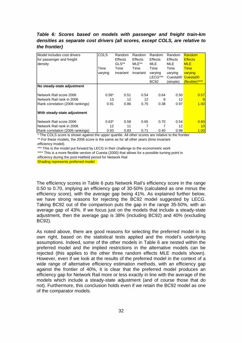
compared. Furthermore, since LECG have put forward the BC92 model, this model is discussed in more detail.

6.1 General discussion of results across methods As noted above, we have strong a priori reasons (based on the model’s flexibility) for selecting our preferred model; and, in addition, appropriate statistical tests show that the model is preferred over models that assume no inefficiency effects, the time varying model put forward by LECG (BC92) and time invariant models. Furthermore, ORR carried out or commissioned other work to verify the results of our preferred model as noted elsewhere in the report. The results were also in line with the regional international efficiency study conducted (as shown in our June 2008 report (ITS/ORR (2008); see also Smith and Wheat (2008)). In addition, we also compared the efficiency scores against a range of other frontier methods (see Table 6) and on this basis judged that the preferred model was in line with the results of other approaches. Table 6 shows Network Rail’s efficiency scores for 2006. The stochastic frontier model scores are shown relative to the frontier as is usual, whilst the COLS scores are shown relative to upper quartile. The latter adjustment is commonly performed by economic regulators, and is a prudent adjustment to put the results on what is probably a more comparable basis to the results of stochastic frontier models (since the COLS44 model does not distinguish inefficiency from noise). Network Rail’s 2006 ranking is also shown, together with the correlation coefficients between the scores for each model against the preferred model (which is shown, with shading, in the final column). Since ORR expressed the view that it is not convinced that Network Rail’s activity is significantly above steady-state by the end of the time period under analysis, the scores before and after the steady-state adjustment are shown. The models in Table 6 include both passenger and freight density as cost drivers since we expect these to impact on costs differently (see also the discussion on sensitivity analysis in section 7). It should also be noted that, whilst two of the models are described as time invariant models, there is a time variant element for Network Rail since the British data has been split to create two firms (relating to the pre- and post-Hatfield period) as discussed earlier.

44 We note that the pooled stochastic frontier model produces the error message, “wrong

skew” in LIMDEP, which may indicate a mis-specification (since the model does not account of the panel structure of the data, and instead treats all 143 data points as separate firms).

32

Table 6: Scores based on models with passenger and freight train-km densities as separate cost drivers (all scores, except COLS, are relative to the frontier) Model includes cost drivers COLS Random Random Random Random Randomfor passenger and freight Effects Effects Effects Effects Effectsdensity GLS** MLE** MLE MLE MLE

Time Time Time Time Time Timevarying invariant invariant varying varying varying

LECG*** Cuesta00 Cuesta00BC92 (simple) (flexible)****

No steady-state adjustment

Network Rail score 2006 0.56* 0.51 0.54 0.64 0.50 0.57Network Rail rank in 2006 13 12 12 9 12 9Rank correlation (2006 rankings) 0.91 0.86 0.75 0.38 0.97 1.00

With steady-state adjustment

Network Rail score 2006 0.63* 0.58 0.65 0.70 0.54 0.60Network Rail rank in 2006 12 11 7 7 12 10Rank correlation (2006 rankings) 0.93 0.83 0.71 0.40 0.98 1.00* The COLS score is shown against the upper quartile. All other scores are relative to the frontier** For these models, the 2006 score is the same as for all other years (time invariant efficiency model).*** This is the model put forward by LECG in their challenge to the econometric work**** This is a more flexible version of Cuesta (2000) that allows for a possible turning point in efficiency during the post-Hatfield period for Network RailShading represents preferred model The efficiency scores in Table 6 puts Network Rail’s efficiency score in the range 0.50 to 0.70, implying an efficiency gap of 30-50% (calculated as one minus the efficiency score), with the average gap being 41%. As explained further below, we have strong reasons for rejecting the BC92 model suggested by LECG. Taking BC92 out of the comparison puts the gap in the range 35-50%, with an average gap of 43%. If we focus just on the models that include a steady-state adjustment, then the average gap is 38% (including BC92) and 40% (excluding BC92). As noted above, there are good reasons for selecting the preferred model in its own right, based on the statistical tests applied and the model’s underlying assumptions. Indeed, some of the other models in Table 6 are nested within the preferred model and the implied restrictions in the alternative models can be rejected (this applies to the other three random effects MLE models shown). However, even if we look at the results of the preferred model in the context of a wide range of alternative efficiency estimation methods, with an efficiency gap against the frontier of 40%, it is clear that the preferred model produces an efficiency gap for Network Rail more or less exactly in line with the average of the models which include a steady-state adjustment (and of course those that do not). Furthermore, this conclusion holds even if we retain the BC92 model as one of the comparator models.

33

Given the above results, we consider that it was appropriate for ORR to use the preferred model (including a steady-state adjustment) as the starting point for its efficiency determination. As discussed further in section 8, ORR benchmarks Network Rail against upper quartile for the preferred model, a conservative assumption that brings the efficiency gap down to 37%.

6.2 The BC92 model put forward by LECG As already noted, we find that the preferred model produces results in line with (and roughly equal to the average of) other models, even if the BC92 model is included as one of the comparators. However, since this model does produce a higher efficiency score than the preferred model, and since LECG put it forward as an alternative in their report, we briefly explain why we have good reasons to select our preferred model over the BC92 model, and indeed to have strong doubts about the BC92 results more generally. Firstly, the BC92 approach is restrictive in that it forces the same direction of efficiency change for all firms over time. This could be a serious limitation if one company has a very different direction of efficiency change over the period (which could be the case for Network Rail). Secondly, as noted above, the BC92 model is nested within our preferred model - which does allow efficiency to vary in different directions for different firms – and the restricted (BC92) model can be very clearly rejected based on appropriate statistical testing45. Further statistical testing shows that, starting from the BC92 model, it is not possible to reject the null hypothesis of time invariant inefficiency, so that the BC92 model cannot be considered a robust model of time varying inefficiency46. As further evidence that the BC92 model may be inappropriate we note that it produces the unexpected result that Network Rail’s efficiency increases every year over the post-Hatfield years (2000 to 2006), which seems unrealistic given the very sharp cost rises over that period (Figure 3). There seems to be little doubt that is was during the post-Hatfield period – that is, during the period of Railtrack’s administration, and the early years after the formation of Network Rail - that efficiency got a lot worse. Indeed all other firms in the sample see increasing efficiency over the whole period as well (the model assumption forces the same direction of change for all firms). In addition, the key traffic density parameters are not statistically significant, and the BC92 model produces a large negative point estimate for the coefficient on the electrification variable. The latter point is important since Network Rail has

45 An LR test rejects the restricted (BC92) model at the 1% level, which is an indication of a

very clear rejection of the BC92 model. 46 In contrast, our preferred time varying efficiency model is clearly preferred over the time

invariant alternative (statistically).

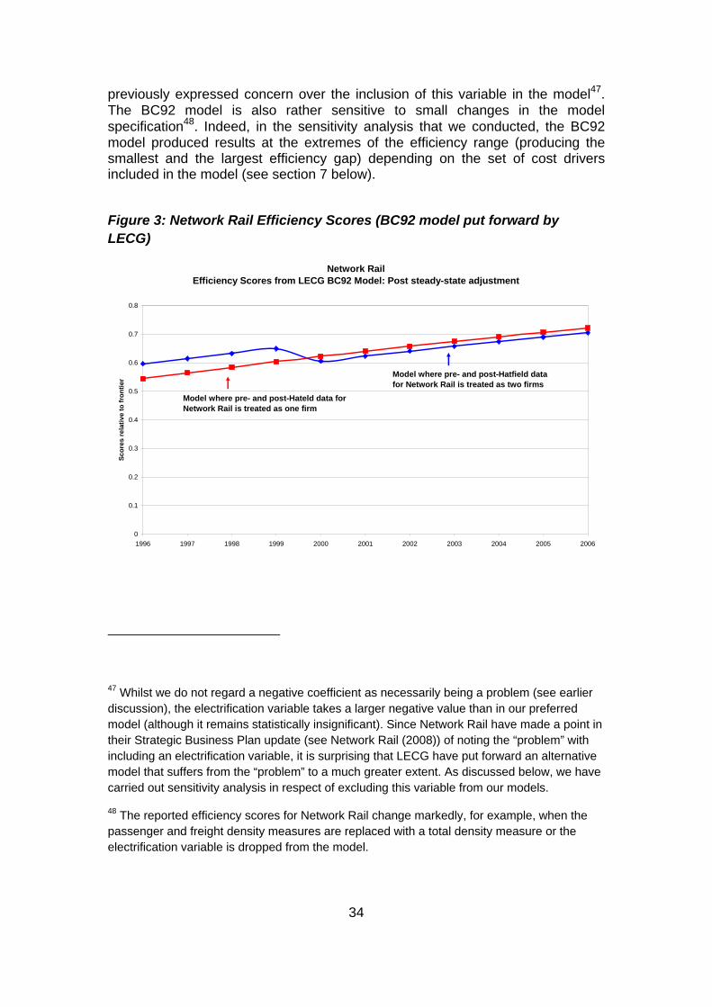
34

previously expressed concern over the inclusion of this variable in the model47. The BC92 model is also rather sensitive to small changes in the model specification48. Indeed, in the sensitivity analysis that we conducted, the BC92 model produced results at the extremes of the efficiency range (producing the smallest and the largest efficiency gap) depending on the set of cost drivers included in the model (see section 7 below).

Figure 3: Network Rail Efficiency Scores (BC92 model put forward by LECG)

Network Rail Efficiency Scores from LECG BC92 Model: Post steady-state adjustment

0

0.1

0.2

0.3

0.4

0.5

0.6

0.7

0.8

1996 1997 1998 1999 2000 2001 2002 2003 2004 2005 2006

Scor

es re

lativ

e to

fron

tier Model where pre- and post-Hatfield data

for Network Rail is treated as two firmsModel where pre- and post-Hateld data for Network Rail is treated as one firm

47 Whilst we do not regard a negative coefficient as necessarily being a problem (see earlier discussion), the electrification variable takes a larger negative value than in our preferred model (although it remains statistically insignificant). Since Network Rail have made a point in their Strategic Business Plan update (see Network Rail (2008)) of noting the “problem” with including an electrification variable, it is surprising that LECG have put forward an alternative model that suffers from the “problem” to a much greater extent. As discussed below, we have carried out sensitivity analysis in respect of excluding this variable from our models.

48 The reported efficiency scores for Network Rail change markedly, for example, when the passenger and freight density measures are replaced with a total density measure or the electrification variable is dropped from the model.

35

It can be seen then, that the weight of evidence from a wide range of models supports the results of the preferred model and that there are strong reasons for selecting the preferred model over the BC92 alternative suggested by LECG. The BC92 model clearly stands out as an outlier. The correlation coefficients between rankings of all firms across models indicate that the BC92 in general produces different rankings for all firms (not just Network Rail), whereas the correlation between the scores and rankings of the preferred model and the other models is reasonably high. The model also produces some rather surprising results in terms of the efficiency scores for Network Rail over time, and can also be rejected based on numerous statistical tests. LECG have put the BC92 model forward without reporting the results of any statistical testing of its properties, or commenting on the reasonableness or otherwise of the results in themselves and as compared to the preferred or other relevant models. 7. SENSITIVITY ANALYSIS In addition to testing alternative efficiency analysis methods, we also ran a number of sensitivities to test the robustness of our preferred model. The results from running the various models and sensitivities discussed in this section demonstrate that our modelling and model selection procedure is robust. First of all, we re-ran all of the models shown in Table 6, replacing the passenger and freight density variables with a measure of total train density. This sensitivity was run in response to a request from Network Rail raised during the various meetings held between ORR, Network Rail and ITS to discuss the modelling process. The results are shown in Table 7 below. The results in Table 7 produce slightly higher efficiency scores (and therefore imply a slightly lower efficiency gap) than those in Table 6, putting the efficiency gap in the range 25% to 54%, with an average gap of 41%. Excluding the BC92 models, which we have reason to doubt as outlined above49, the efficiency gap ranges from 33% to 49% (average of 41%), or 33% to 41% (average of 37%) if only the most favourable models (i.e. those that include a steady-state adjustment) are included. The preferred model, with an efficiency gap of 40% against the frontier, is again broadly in the middle of the range of estimates in Table 7.

49 The comments above apply also to the total train density version of the BC92 model. Indeed, we note here that the BC92 model defines the extreme upper and lower bounds of the efficiency gap, depending on the cost variable used, which is a further indication of its instability.

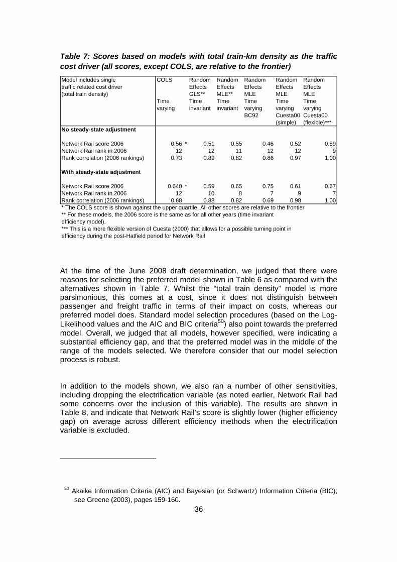
36

Table 7: Scores based on models with total train-km density as the traffic cost driver (all scores, except COLS, are relative to the frontier) Model includes single COLS Random Random Random Random Randomtraffic related cost driver Effects Effects Effects Effects Effects(total train density) GLS** MLE** MLE MLE MLE

Time Time Time Time Time Timevarying invariant invariant varying varying varying

BC92 Cuesta00 Cuesta00(simple) (flexible)***

No steady-state adjustment

Network Rail score 2006 0.56 * 0.51 0.55 0.46 0.52 0.59Network Rail rank in 2006 12 12 11 12 12 9Rank correlation (2006 rankings) 0.73 0.89 0.82 0.86 0.97 1.00

With steady-state adjustment

Network Rail score 2006 0.640 * 0.59 0.65 0.75 0.61 0.67Network Rail rank in 2006 12 10 8 7 9 7Rank correlation (2006 rankings) 0.68 0.88 0.82 0.69 0.98 1.00* The COLS score is shown against the upper quartile. All other scores are relative to the frontier** For these models, the 2006 score is the same as for all other years (time invariant efficiency model).*** This is a more flexible version of Cuesta (2000) that allows for a possible turning point in efficiency during the post-Hatfield period for Network Rail At the time of the June 2008 draft determination, we judged that there were reasons for selecting the preferred model shown in Table 6 as compared with the alternatives shown in Table 7. Whilst the “total train density” model is more parsimonious, this comes at a cost, since it does not distinguish between passenger and freight traffic in terms of their impact on costs, whereas our preferred model does. Standard model selection procedures (based on the Log-Likelihood values and the AIC and BIC criteria50) also point towards the preferred model. Overall, we judged that all models, however specified, were indicating a substantial efficiency gap, and that the preferred model was in the middle of the range of the models selected. We therefore consider that our model selection process is robust. In addition to the models shown, we also ran a number of other sensitivities, including dropping the electrification variable (as noted earlier, Network Rail had some concerns over the inclusion of this variable). The results are shown in Table 8, and indicate that Network Rail’s score is slightly lower (higher efficiency gap) on average across different efficiency methods when the electrification variable is excluded.

50 Akaike Information Criteria (AIC) and Bayesian (or Schwartz) Information Criteria (BIC);

see Greene (2003), pages 159-160.

37

Table 8: Scores including and excluding the electrification variable as a cost driver (all scores, except COLS, are shown against the frontier) Model includes cost drivers COLS Random Random Random Random Averagefor passenger and freight Effects Effects Effects Effects Scoredensity GLS** MLE** MLE MLE Across

Time Time Time Time Time Methodsvarying invariant invariant varying varying

Cuesta00 Cuesta00(simple) (flexible)***

NR 2006 score - preferred specification 0.63 * 0.58 0.65 0.54 0.60 0.60

NR 2006 score - excluding electrification 0.59 * 0.55 0.57 0.51 0.51 0.54variable

* For comparative purposes the COLS score is shown against the upper quartile** For these models, the 2006 score is the same as for all other years (time invariant efficiency model).*** This is a more flexible version of Cuesta (2000) that allows for a possible turning point in efficiency during the post-Hatfield period for Network Rail We also ran numerous other model specifications, for example, including switch and stations density (though noting the possible data quality issues with these variables); and testing models specified in terms of track-km rather than route-km. In all cases the resulting efficiency scores were very close to those of the preferred model, and in some cases where substantially lower. In addition, in some cases the alternative models run performed less well in terms of the size and significance of the parameter estimates. 8. ORR’S USE OF THE ECONOMETRIC ANALYSIS IN PR2008 It can be seen from the discussion above that there are good reasons for selecting the preferred model in its own right, based on the statistical tests applied and the model’s underlying assumptions. Indeed, the general consensus of evidence here is one of a substantial efficiency gap across all methods and the preferred model produces results in the middle of the range of models estimated. In our view it is therefore appropriate for ORR to use the results of this model as the starting point for its efficiency determination. Furthermore, since the computation of efficiency scores relative to upper quartile is normally only applied in the case of deterministic frontier approaches (in particular COLS), which do not take account of random noise, the use of an efficiency gap measured against upper quartile in this case (for a stochastic

38

frontier model) reflects ORR’s aim to use a conservative estimate of Network Rail’s efficiency gap as its starting point (see ORR (2008)51). In our view, ORR’s starting point for its efficiency determination is therefore a reasonable one, based on the econometric work carried out. The econometric results are also supported by the regional international econometric study (see ORR/ITS (2008)). From the starting point of a 37% efficiency gap, ORR then makes a further discounting assumption that two thirds of the gap can be closed over CP4. Furthermore, ORR has combined the results of the econometric work with other evidence in arriving at its draft efficiency determination. We therefore consider that, in general terms, ORR has made appropriate use of the econometric work in its analysis, although ITS did not review the other evidence commissioned / produced by ORR, and was not involved in the details of the process by which ORR reached its draft efficiency determination. This process resulted in the efficiency gap from the preferred econometric model of 37% being scaled down to an efficiency target for maintenance and renewals in CP3 of 22% (see ORR (2008)52) and, of course, required ORR to exercise its regulatory judgement. 9. CONCLUSIONS This document has explained the model selection process and shown that the preferred econometric model is robust, both in its own right, and in the context of the vast array of other methods that we have applied to this dataset. Where relevant, we have referred to and refuted the challenges raised by LECG and Horton 4 Consulting during their work over the summer of 2008. For further details on the latter, see our response document (Smith and Wheat, 2008)). As noted earlier in the report, during our work some areas of analysis were outside the scope of ITS’s remit (for example, collating evidence on the extent to which companies were above or below steady-state). In these areas we took advice from ORR, and where this was done it is indicated in the relevant section of the report. LECG’s assertion that a “fix” is required in order for the model to produce an estimate is shown to be incorrect. Furthermore, we have shown that the method used to derive the variance co-variance matrix (from which the standard errors and hence the means of determining the precision of the estimates are derived) is an accepted and widely used approach, and that alternative testing procedures also provide support for the method used. The preferred model also produces

51 See, for example, page 115-116. 52 See page 141.

39

plausible estimates for the model parameters, which are also statistically significant at the usual levels of significance53. It also produces a plausible time path of efficiency for Network Rail over the period: that is, improving modestly after privatisation (even after making the steady-state adjustment), deteriorating after Hatfield, before improving during CP3. As noted, our preferred model also produces similar efficiency estimates for Network Rail to those from the other methods that we have tested, and there is also strong conformity of efficiency rankings (for all firms) across the different methods applied. LECG’s assertion that the Cobb-Douglas functional form adopted in our study violates economic theory in the multiple output case is shown to be incorrect (see Smith and Wheat (2008). LECG’s assertion is based on a single quote from one textbook, which has been taken out of the context of the wider theoretical and empirical literature, and indeed even the book from which the quote is taken. It is clear from the literature that the multiple output Cobb-Douglas cost function does not violate any required theoretical property of a cost function in a regulated industry, such as railways, where output levels are typically assumed to be exogenously determined (see, for example, Klein (1953), Nerlove (1965), and Coelli and Perelman (2000)). Indeed, in Smith and Wheat (2008) we show that this functional form is widely used in both academic and regulatory studies. The appropriate functional form is, instead, an issue for econometric testing and, as noted in the ITS/ORR June 2008 report, we have tested the Cobb-Douglas model and found it to be preferred to the alternatives. Furthermore, LECG have themselves utilised a multiple-output Cobb-Douglas cost function in their recent (2005) study of postal delivery office efficiency, so it extremely puzzling that they have raised this issue in criticism of our work. This functional form has also been used by OFWAT, as LECG note in their 2005 study. In all of the other areas of concern raised by the consultants – which include data quality, possible omitted variables, and the modelling of railways out of steady-state, these have either been directly addressed in the modelling approach, or ORR has done other work to verify the appropriateness of the approach taken (it was recognised that that further work with regard to omitted variables and quantifying the extent to which railways are out of steady-state was outside ITS’s remit, and in these areas we took advice from ORR). Ultimately, as well as highlighting the strong reasons for selecting the preferred model (in its own right) as the starting point for ORR’s analysis, we also show that this model produces an efficiency gap in the middle of the range of estimates resulting from the various models estimated and sensitivity analysis conducted. Furthermore, ORR benchmarks Network Rail against the upper quartiles, and not

53 As demonstrated by the standard errors derived from the variance co-variance matrix, and

alternative testing procedures as noted.

40

the frontier, which is a conservative approach given that the preferred model is a stochastic frontier model. In our view, ORR’s starting point for its efficiency determination is therefore a reasonable one, based on the econometric work carried out. The econometric results are also supported by the regional international econometric study (see ITS/ORR (2008)). From the starting point of a 37% efficiency gap, ORR then makes a further discounting assumption that two thirds of the gap can be closed over CP4. Furthermore, ORR has combined the results of the econometric work with other evidence in arriving at its draft efficiency determination. We therefore consider that, in general terms, ORR has made appropriate use of the econometric work in its analysis, although ITS did not review the other evidence commissioned / produced by ORR, and was not involved in the details of the process by which ORR reached its draft efficiency determination. This process resulted in the efficiency gap from the preferred econometric model of 37% being scaled down to an efficiency target for maintenance and renewals in CP3 of 22% (see ORR (2008)54) and, of course, required ORR to exercise its regulatory judgement.

54 See page 141.

41

ANNEX 1: MAINTENANCE AND RENEWALS ONLY MODELS As noted above, our preferred approach was to model maintenance and renewals together. In this annex we briefly report the results of the separate maintenance-only and renewals-only models that we ran (some details were provided in our June report). These results support the findings from the preferred, combined maintenance and renewals models set out in the main body of the report.

A1.1 Maintenance-only models The parameter estimates for the flexible Cuesta00 maintenance-only model are shown in Table 9 below. Note that this model is slightly different from that shown in the June 2008 report, since the British data is split into two firms (one before and one after Hatfield), whereas the June 2008 report was based on treating the British data as a single firm. In general we have found that the results are not substantially impacted by the decision to split (or not) the British data, but we have chosen to the show the results based on the split sample so that they are consistent with the approach taken for the total cost models55.

Table 9: Maintenance cost parameter estimates

Coefficients SignificanceCONSTANT 5.477 ***ROUTE 0.843 ***PASSDR 0.136 **FRDR 0.157 ***SING -0.715 ***ELEC 0.073TIME 0.047 ***TIME2 -0.003 **Lambda 3.668 ***Sigma(u) 0.337 **** Significant at the 10% level. ** Significant at the 5% level*** Significant at the 1% level (all based on the standard errors taken from the varianceco-variance matrix

Flexible Cuesta00 stochastic frontier modelMaintenance costs

Raw data model

55 The overall elasticity with respect to volume is similar across the two approaches as are

most of the other coefficients. The time trend is slightly different however.

42

The model performs well statistically in terms of the signs, magnitudes and statistical significance of the parameter estimates. In terms of the efficiency results, the model produces an efficiency score for Network Rail of 0.59 in 2006 which is in line with the results of the total cost models. Against upper quartile, the model shows an efficiency score of 0.65 (as against 0.66 for the equivalent model with the British data treated as a single firm)56. These results therefore provide support for the total maintenance and renewal cost models shown in the main body of the report. There is also strong conformity in efficiency scores and rankings for Network Rail across the alternative efficiency analysis methods (as shown in Table 10 below). Once again, we note that the BC92 model stands out as the outlier, this time producing by far the smallest efficiency score (so by far the largest efficiency gap).

Table 10: Maintenance efficiency scores across method (scores shown against frontier, except for COLS) Model includes cost drivers COLS Random Random Random Random Randomfor passenger and freight Effects Effects Effects Effects Effectsdensity GLS** MLE** MLE MLE MLE

Time Time Time Time Time Timevarying invariant invariant varying varying varying

BC92 Cuesta00 Cuesta00(simple) (flexible)***

With steady-state adjustment

Network Rail score 2006 0.70 * 0.64 0.65 0.41 0.52 0.59Network Rail rank in 2006 11 13 11 12 12 11

* For comparative purposes the COLS score is shown against the upper quartile** For these models, the 2006 score is the same as for all other years (time invariant efficiency model).*** This is a more flexible version of Cuesta (2000) that allows for a possible turning point in efficiency during the post-Hatfield period

A1.2 Renewals -only models The parameter estimates for the flexible Cuesta00 renewals-only models (with and without steady-state adjustment) are shown in Table 11 below. With the exception of the electrification variable, the coefficients have the right sign, although not all variables are statistically significant at the 5% level. In general, the renewals only model performs less well statistically than either the total M&R model or the maintenance model. This might be expected as renewals are more lumpy than maintenance and, hence, renewals costs are harder to model.

56 The score against frontier for that model in 2006 is 0.64.

43

Possible definitional differences (between maintenance and renewal) may also impact the results, although we have no evidence that these are substantial.

Table 11: Renewals cost parameter estimates

Coefficients Significance Coefficients SignificanceCONSTANT 4.90267 *** 4.910 ***ROUTE 1.33886 *** 1.383 ***PASSDR 0.343322 * 0.319 *FRDR 0.274347 *** 0.192SING -1.51504 *** -1.645 ***ELEC -0.385418 *** -0.485 ***SWITCH 0.19143 * 0.134TIME 0.11508 *** 0.115 ***TIME2 -0.00763429 *** -0.008 **** Significant at the 10% level. ** Significant at the 5% level*** Significant at the 1% level (all based on the standard errors taken from the varianceco-variance matrix

Flexible Cuesta00 stochastic frontier modelRenewal costs

Raw data model Steady-state model

In particular, the coefficient on the route-km variable (at 1.38 in the steady-state model) is higher than might be expected based on the received literature (indicating substantial diseconomies of scale), given that the cost base here only includes infrastructure costs. As noted above, the electrification variable also takes a negative sign (and is statistically significant). It may be that this variable is picking up the effects of other quality factors that are correlated with electrification, for example age. However, the magnitude of the coefficient suggests that costs fall quickly with increased electrification. If the electrification variable is dropped, Network Rail’s efficiency score falls substantially. The efficiency scores for Network Rail in 2006 are 0.58 and 0.77 for the raw renewals and steady-state renewals models respectively. The relevant scores against upper quartile are 0.61 and 0.84 respectively. Therefore, broadly speaking these models provide support for the total maintenance and renewals models and maintenance-only models reported earlier, at least for the unadjusted cost data. However, the steady-state adjusted model shows a higher efficiency score than for the total cost models. In this respect, it should also be noted that for Network Rail the steady-state adjusted model suggests that the company’s efficiency score is deteriorating throughout CP3, which is unexpected; whereas the unadjusted renewals cost model produces a more sensible time path of inefficiency (i.e. rising towards the end of CP3), and more in line with the total cost models reported earlier. A comparison of the results across different efficiency methods is shown in Table 12 below. There is more variation in the scores and rankings across methods here but, in general these results indicate a substantial efficiency gap. If we

44

ignore the very low scores of the random effects (GLS) models, and also the BC92 model for the reasons described earlier, the average efficiency gap resulting from Table 14 is 37%, which is in line with the gap used by ORR as the starting point for its efficiency analysis. Thus, whilst the renewals models do not perform as well as the other models, they provide general support for the preferred total cost models.

Table 12: Renewals only efficiency scores across method (scores shown against frontier, except COLS) Model includes cost drivers COLS Random Random Random Random Randomfor passenger and freight Effects Effects Effects Effects Effectsdensity GLS** MLE** MLE MLE MLE

Time Time Time Time Time Timevarying invariant invariant varying varying varying

BC92 Cuesta00 Cuesta00(simple) (flexible)***

No steady-state adjustment

Network Rail score 2006 0.54 * 0.28 0.51 0.70 0.54 0.58Network Rail rank in 2006 13 11 8 5 6 5

With steady-state adjustment

Network Rail score 2006 0.62 * 0.35 0.73 0.86 0.77 0.77Network Rail rank in 2006 9 9 6 5 5 5

* For comparative purposes the COLS score is shown against the upper quartile** For these models, the 2006 score is the same as for all other years (time invariant efficiency model).*** This is a more flexible version of Cuesta (2000) that allows for a possible turning point in efficiency during the post-Hatfield period

45

REFERENCES Barros, C.P. (2005), ‘Governance and Incentive Regulation in Defence Industry

Enterprises: A Case Study’, European Journal of Law and Economics, vol. 20, pp. 87-97.

Battese, G.E. and Coelli, T.J. (1992), ‘Frontier Production Functions and the Efficiencies of Indian Farms Using Panel Data from ICRISAT’s Village Level Studies’, Journal of Quantitative Economics, vol. 5, pp. 327-348.

Battese, G.E. and Coelli, T.J. (1995), ‘A Model for Technical Inefficiency Effects in a Stochastic Frontier Production Function for Panel Data’, Empirical Economics, vol. 20, pp. 325-332.

BSL (2008), Rail Infrastructure Cost Benchmarking: Brief LICB-gap analysis and cost driver assessment, final report (April 2008).

Coelli, T. (1996), ‘A Guide to FRONTIER Version 4.1: A Computer Program for Frontier Production Function Estimation’, CEPA Working Paper 96/07, Department of Econometrics, University of New England, Armidale.

Coelli, T. and Perelman, S. (2000), ‘Technical Efficiency of European Railways: A Distance Function Approach’, Applied Economics, vol. 32, pp. 1967-1976.

Coelli, T., Rao, D.S.P, O’Donnell, C.J. and Battese, G.E. (2005), An Introduction to Efficiency and Productivity, 2nd edition, New York, Springer.

Cuesta, R. A. (2000). ‘A Production Model with Firm-Specific Temporal Variation in Technical Inefficiency: With Application to Spanish Dairy Farms’ Journal of Productivity Analysis, 13, pp. 139-158.

Dougherty, C. (1992), Introduction to Econometrics, Oxford University Press.

Eeckaut, P.V., Tulkens, H. and Jamar, M. (1993), ‘Cost Efficiency in Belgian Municipalities’, in Fried, H.O., Lovell, C.A.K. and Schmidt, S.S., eds., The Measurement of Productive Efficiency, New York, Oxford University Press.

Farsi, M. and Filippini, M. (2006), ‘An Analysis of Efficiency and Productivity in Swiss Hospitals’, Swiss Journal of Economics and Statistics, vol. 142, issue 1, pp. 1-37.

Greene, W.H. (2003), Econometric Analysis: fifth edition, Prentice Hall.

Greene, W. (2005), ‘Reconsidering heterogeneity in panel data estimators of the stochastic frontier model’, Journal of Econometrics, vol. 126, pp. 269-303.

46

Hasenkamp, G. (1976), ‘A Study of Multiple-Output Production Functions: Klein’s Railroad Study Revisited’, Journal of Econometrics, vol. 4, pp. 253-262.

Horton 4 Consulting (2008), International Efficiency Benchmarking in the Network Rail 2008 Periodic Review: ORR’s Draft Determination, report produced as part of PR2008, 31 July 2008.

ITS/ORR (2008), International Benchmarking of Network Rail’s Maintenance and Renewal Costs, joint report written by Andrew Smith and Phill Wheat (ITS) and Hannah Nixon (ORR) as part of PR2008, June 2008.

Klein, W.H. (1953), A Textbook of Econometrics, Row, Peterson and Company.

Kumbhakar, S.C. and Heshmati, A. (1995), ‘Efficiency Measurement in Swedish Dairy Farms: An Application of Rotating Panel Data’, Journal of Agricultural Economics, vol. 77, no. 3, pp. 660-674.

Kumbhakar, S.C. and Hjalmarsson, L. (1995), ‘Labour-Use Efficiency in Swedish Social Insurance Offices’, Journal of Applied Econometrics, vol. 10, pp. 33-47.

Kumbhakar, S.C. and Lovell, C.A.K. (2000), Stochastic Frontier Analysis, Cambridge University Press, Cambridge UK.

LECG (2005), Future Efficient Costs of Royal Mail’s Regulated Mail Activities, August 2005.

LECG (2008), Assessment of the ITS/ORR Econometric Models, report produced as part of PR2008, 4 September 2008.

Lovell, C.A.K. (1993), ‘Production Frontiers and Production Efficiency’, in Fried, H.O., Lovell, C.A.K. and Schmidt, S.S., eds., The Measurement of Productive Efficiency, New York, Oxford University Press.

Mulatu, A. and Crafts, N.F.R. (2005), ‘Efficiency Among Private Railway Companies in a Weakly Regulated System: The Case of Britain’s Railways in 1893-1912’, Department of Economic History Working Paper No. 08/05, London School of Economics.

Nerlove, M. (1965), Estimation and Identification of Cobb-Douglas Production Functions, Rand McNally and Company, Chicago.

Network Rail (2008), Network Rail: Response to ORR’s Draft Determinations: Periodic Review 2008, September 2008.

Orea, L. and Kumbhakar (2004), ‘Efficiency measurement using a latent class stochastic frontier model’, Empirical Economics, 29, 169-183.

ORR (2008), Periodic Review 2008: Draft Determinations, June 2008.

47

Pitt, M.M. and Lee, L.F. (1981), ‘Measurement and Sources of Technical Inefficiency in the Indonesian Weaving Industry’, Journal of Development Economics, 9,43-64.

Schmidt, P. and Sickles, R.C. (1984), ‘Production Frontiers and Panel Data’, Journal of Business & Economic Statistics, vol. 2 (4), pp 367-374.

Smith, A.S.J. and Wheat, P.E. (2008), A Response to the LECG and Horton 4 Consulting Reports on the ITS/ORR International Benchmarking Study (Based on the LICB Dataset), report written as part of PR2008, October 2008.

Sumicsid (2007), Project Gerner / AS6: Development of Benchmarking Models for German Electricity and Gas Distribution: Final Report.

UIC (2007), Lasting Infrastructure Cost Benchmarking (LICB): 10 years of Benchmarking 1996-2005.

Zarembka, P. (1968), ‘Functional form in demand for money’, Journal of the American Statistical Association, vol. 63 (322): pp. 502-511