International asset allocation in presence of systematic cojumps

This version: June 2016

Abstract This paper provides a new partial explanation of the home bias phenomenon in international asset holdings from an investigation of intraday jumps and cojumps. Using intraday index-based data for exchange-traded funds, we document evidence of significant systematic jump risks in international equity markets, which drive investors to reduce the proportion of foreign assets in their diversified portfolios. In addition, we show a negative link between the demand of foreign assets and the number of cojumps between domestic and foreign assets when considering the composition of the optimal portfolio in the sense of mean-variance and mean-CVaR approaches. Keywords: systematic jump risk, cojumps, home bias

2

1 Introduction

This paper contributes to the literature on international home bias puzzle by examining whether

jump and cojump risks explain a part of this phenomenon. It is now well established in the

finance literature that price discontinuities or jumps should be taken into account when studying

asset price dynamics and allocating funds across assets (Bekaert et al., 1998; Das and Uppal,

2004; Guidolin and Ossola, 2009). In this regard, the recent development of non-parametric jump

identification tests has enabled jump detection in financial asset prices. The seminal works in this

area include Barndorff-Nielsen and Shephard (2004, 2006a) who test for the presence of jumps

at the daily level using measures of bipower variation. The same family of intraday jump

identification procedures includes the tests developed by, among others, Jiang and Oomen

(2008), Andersen et al. (2012), Corsi et al. (2010), Podolskij and Ziggel (2010), and Christensen

et al. (2014). Andersen et al. (2007) and Lee and Mykland (2008) have developed techniques to

identify intraday jumps using high frequency data. All of these jump detection techniques

provide empirical evidence in favor of the presence of asset price discontinuities or jumps.

More recently, researchers are interested in studying cojumps between assets (Dungey et

al., 2009; Lahaye et al., 2010; Dungey and Hvozdyk, 2012; Pukthuanthong and Roll, 2015; Ait-

Sahalia and Xiu, 2016). For instance, Gilder et al. (2012) examine the frequency of cojumps

between individual stocks and the market portfolio, and find a tendency for a relatively large

number of stocks to be involved in systematic cojumps. Lahaye et al. (2010) show that asset

cojumps are partially associated with new macroeconomic announcements. Ait-Sahalia et al.

(2015) develop a multivariate Hawkes jump-diffusion model to capture jumps propagation over

time and across markets. They provide strong evidence for jumps to arrive in clusters within the

same market and to propagate to other international markets. Bormetti et al. (2015) find that

3

Hawkes one-factor model is more suitable to capture the high synchronization of jumps across

assets than the multivariate Hawkes model.

Our study furthers the current literature in two key ways. First, it empirically investigates

cojumps between international equity markets. Second, we show their impact on international

asset allocation. Specifically, we propose the systematic jumps partially explain home bias

phenomenon. Modern portfolio theory suggests that international diversification is an effective

way to minimize portfolio risks given that international assets are often less correlated and driven

by different economic factors. However, one might expect that systematic cojumps can lead to an

increase in the correlation between these international assets and thus affect negatively the

benefit from international diversification. Inversely, if price jumps are not systematic (i.e., they

are specific to a particular market due to asset-specific events which are uncorrelated with

market movement), they are categorized as idiosyncratic jumps and will not affect portfolio

allocation decisions in an international setting.

Accordingly, a risk-averse investor who holds an international portfolio is exposed to two

types of jump risks: systematic jump risk or cojumps (jumps common to all markets) and

idiosyncratic jump risk (jumps specific to one market). If the investor’s portfolio is well

diversified, the idiosyncratic jump risk will be reduced or even eliminated. On the other hand, the

systematic jump risk could not be eliminated through diversification, thus making its

identification central to asset pricing, asset allocation and portfolio risk hedging. Its presence and

contribution to the global portfolio risk also represent a good risk indicator for investors when

selecting portfolio composition among all available assets.

Two hypotheses are examined in this paper. The first posits that international equity

markets experience cojumps and a part of the jump risk is rather systematic. The second posits

4

that the systematic jump risk could partially explain the lack of international asset holdings or the

home bias, observed in global equity markets. If the systematic cojumps risk exists between

international equity markets, we would expect an increase in the cross-market linkages and thus

a decrease of diversification benefits. As a result, investors would prefer investing in domestic

assets.

Our empirical tests rely on the use of intraday returns for three dedicated international

exchange-traded funds (ETFs) – SPY, EFA, and EEM – which respectively aim to replicate the

performance of three international equity market indices: S&P 500, MSCI EAFE (Europe,

Australasia and Far East), and MSCI Emerging Markets.1 We use the technique proposed by

Andersen et al. (2007) and Lee and Mykland (2008) to empirically identify all intraday jumps

and cojumps of the three funds from January 2008 to October 2013. Lee and Mykland (2008)

show that the power of their non-parametric jump identification test increases with the sampling

frequency and that spurious detection of jumps is negligible when high frequency data are used.

Unlike Ait-Sahalia et al. (2015) who use low frequency data to study the dynamics of jumps, we

employ a bivariate Hawkes model to reproduce the time clustering features of intraday jumps

and the dynamics of their propagation across markets. The application of the Hawkes process is

particularly novel in the finance literature as it allows us to capture the dependency between the

occurrences of jumps which cannot be reproduced by, for example, the standard Poisson process,

owing to the hypothesis of independence of the increments (i.e., the numbers of jumps on

disjoint time intervals should be independent).

1 S&P 500 index is used as a proxy for the US market. MSCI EAFE index is the benchmark for developed markets excluding the US and Canada, whereas the MSCI Emerging Markets is used to capture the performance of emerging equity markets.

5

We also assess the impact of systematic jumps on international portfolio allocation

(second hypothesis) by considering a domestic risk-averse investor who selects the portfolio

composition based on one domestic asset and two foreign assets to minimize the portfolio risk,

while requiring a minimum expected return. As investors are concerned about negative

movements of asset returns, we take the risk of extreme events into account by using the

Conditional Value-at-Risk or CVaR (Rockafellar and Uryasev, 2000) as a risk measure in our

portfolio allocation problem. Unlike the standard mean-variance framework, which typically

underestimates the risk of large movements of asset returns, the mean-CVaR approach allows us

to provide a fairly accurate estimate of the downside risk induced by systematic negative jumps

of asset returns. Once the optimal portfolio composition is determined, we analyze how jumps

and cojumps affect investor demand for domestic and foreign assets. Our results show evidence

of a negative and significant link between the demand for foreign assets and the intensity of

cojumps between the domestic and foreign markets. We also find a negative effect of cross-

market cojumps on the conditional diversification benefit measure.

The remainder of the paper is organized as follows. Section 2 introduces the jump and

cojump identification techniques used in our study. Section 3 presents the portfolio allocation

problem in mean-variance and mean-CVaR frameworks. Section 4 describes the data. Section 5

discusses our main empirical findings. Section 6 concludes the paper.

2 Jump and cojump detection methodology

2.1 Jump test statistics

To explain the basic idea behind the jump detection procedures used in this paper, we begin with

the Barndorff-Nielsen and Shephard (2004, 2006a) non-parametric jump test based on two

6

measures of price variation: realized variance (RV) and bipower variation (BV). The first

measure captures the variation in the prices coming from both continuous and jump components

of the total price variation process, while the second one is jump robust and only seizes variation

coming from the continuous part of the process. This test has been largely applied in past studies

to determine if a day (or a given time window) contains price jumps.

Assume that the logarithm of the price of an asset can be generated by the following

jump-diffusion model (Merton 1976):

(1)

where represents the time-varying drift component, represents the time-varying

volatility component of the asset price, and is a standard Brownian motion. denotes the

time-varying jump component of the process. stands for the size of jumps and is a counting

process independent of . We consider M equidistant observations of the logarithm of the price

at day t: . The kth intraday return of day t is then defined by:

(2)

The realized variance of the price at day t, which converges to the integrated variance

(IV) plus a jump component as the sampling frequency of the price observations increases

, is calculated as following:

(3)

(4)

tp

, 0t t t t t tdp µ dt dW dJ t Tσ κ= + + ≤ ≤

tµ dt t tdWσ

tW t tdJκ

tκ tJ

tW

( ), 1,...,t k k Mp

=

, , , 1, 1,...,t k t k t kr p p k M−= − =

( )M → ∞

2,

1

M

t t kk

RV r=

=∑

2 2,1

1

tNtM

t s t jtj

RV dsσ κ→∞

−=

→ +∑∫

7

where represents the number of within day jump at day t and denotes the magnitude of jth

jump at day t.

Barndorff-Nielsen and Shephard (BNS) also propose a jump robust measure of the

integrated variation, called the bipower variation (BV), which converges to the integrated

variance as the sampling frequency of the price observations increases :

(5)

(6)

In this setting, the difference between realized variance and bipower variation is used to

estimate the sum of jumps within a day. We consider the relative jump measure which

quantifies the contribution of jumps to the total within-day variation of the process, such as:

We also introduce a modified form of BNS test statistic proposed by Huang and Tauchen

(2005) to identify days with at least one jump. Huang and Tauchen (2005) prove that this

particular form of the BNS test outperforms the other forms of BNS test applied in the financial

literature in terms of size and power. The test statistic of Huang and Tauchen (HT) is given by:

(7)

tN ,t jκ

( )M → ∞

, 1 ,22 1

M

t t k t kk

MBV r r

M

π−

=

=− ∑

2

1

tM

t s

t

BV dsσ→∞

−

→ ∫

tRJ

t tt

t

RV BVRJ

RV

−=

2

2

15 max 1,

2

tt

t

t

RJZ

QV

M BV

π π=

+ −

8

where (8)

The null hypothesis of absence of jumps at day t is rejected with a probability of if

, where represents the inverse of the standard normal cumulative distribution

function evaluated at a cumulative probability of .

By construction, the previous tests (BNS or HT) can only check for the discontinuity of

asset prices at a daily level and are generally applied to determine if a day (or a given time

window) contains price jumps, but they do not provide further information about the number, the

time and the size of the jumps that occurs during a given time window. Thus, a test statistic is

required in order to identify all intraday jumps for a given day and to determine the occurrence

time and the size of each jump. In the related literature, there are essentially two procedures to

identify intraday jumps, proposed by Andersen et al. (2007, henceforth ABD) and Lee and

Mykland (2008, henceforth LM). The LM and ABD procedures use the same test statistic, but

differ on the choice of the critical value. ABD assumes that the test statistic is asymptotically

normal, whereas LM provides critical value from the limit distribution of the maximum of the

test statistic. Moreover, Dumitru and Urga (2012) show that intraday jump tests of LM and ABD

outperform other test procedures when price volatility is not high.

The LM test statistic ( ) compares the current asset return with the bipower variation

calculated over a moving window with a given number of preceding observations. It tests at time

k whether there was a jump from k-1 to k and is defined as:

(9)

2

, 3 , 2 , 1 ,42 3

M

t t k t k t k t kk

MQV M r r r r

M

π− − −

=

= − ∑

1 α−

11tZ α−−> Φ 1

1 α−−Φ

1 α−

,t kL

,,

,ˆt k

t kt k

rL

σ=

9

where (10)

In Eq. (9), refers to the realized bipower variation calculated for a window of K

observations and provides a jump robust estimator of the instantaneous volatility. Lee and

Mykland (2008) emphasize that the window size K should be chosen in a way that the effect of

jumps on the volatility estimation disappears. They thus suggest to choose the window size K

between and , where M is the number of observations in a day. Under the null

hypothesis of absence of jumps at anytime in the interval [k-1, k], the LM statistic is

asymptotically distributed as:

(11)

where has a cumulative distribution function, , andand are given

by:

(12)

and (13)

The null hypothesis of absence of jumps is rejected for a given significance level if

.

( )1

2

, , 1 ,2

1ˆ

2

k

t k t j t jj k K

r rK

σ−

−= − +

=− ∑

,ˆ t kσ

252 M× 252 M×

,t k M M

M

L C

Sξ→∞−

→

ξ ( ) ( )exp xP x eξ −≤ = MC MS

( ) ( ) ( )( )( )

2log log log log

2 2logM

M MC

c c M

π += −

( )1

2 logMS

c M= 2

cπ

=

α

( )( ), log log 1t k M ML S Cα> − − − × +

10

On the other hand, the ABD test statistic is assumed to be normally distributed in the

absence of jumps. A jump is detected with the ABD test on day t in intraday interval k if the

following condition is satisfied:

(14)

where represents the inverse of the standard normal cumulative distribution function

evaluated at a cumulative probability of and , where represents the daily

significance level of the test.

In our study, we identify intraday jumps by relying on the intraday procedure of LM-

ABD. A jump is detected with the LM-ABD test on day t in intraday interval k when:

(15)

The threshold value is calculated for different significance levels. For a daily

significance level of 5% and a sampling frequency of 5 minutes (which corresponds to 77

intraday returns per day in our study), we obtain a threshold value of 3.40 and 4.40 using ABD

and LM methods, respectively. In our study, we combine both procedures by taking an

intermediate threshold value equal to 4.2

2.2 Cojump identification procedure

2 This threshold value is also employed by Bormetti and al. (2015). We also consider different threshold values (3 and 5). However, the results remain intact.

, 1

121

t k

t

r

BVM

β−

−> Φ

1

12

β−

−Φ

12

β− ( )1 1Mβ α− = − α

,

,ˆt k

t k

rθ

σ>

θ

11

A cojump exists when financial asset returns jump simultaneously. We use a two-step procedure

to identify a cojump for a pair of assets. First, we detect the intraday jumps of each asset using

the LM-ABD method described in subsection 2.1. We then apply the following co-exceedance

rule to detect a cojump (Bae et al., 2003):3

, , , ,

, , , ,ˆ ˆ

1: a cojump between assets i and j 1 1

0:nocojump i t k j t k

i t k j t k

r rθ θ

σ σ

> >

× =

(16)

Thus, we define cojumps as simultaneous significant jumps based on univariate tests of

LM-ABD. Other techniques have recently been proposed to identify cojumps in the multivariate

context using a single cojump test statistic such as those proposed by Barndorff-Nielsen and

Shephard (2006b), Jacod and Todorov (2009), and Bollerslev et al. (2008). For instance, a

cojump test proposed by Bollerslev et al. (2008) recognizes the role of covariance and thus is

based on the use of cross products in a panel of intraday stock returns to measure this covariance.

However, the power of their test relies on how efficiently this comovement is measured. The

return-based estimator, which is the cross product of intraday returns, may not be the best

covariance estimator. The cojump test based on co-exceedance rule is appropriate for our context

because it presents simple estimates of precisely timed cojumps with a relatively narrow range of

intraday data. Moreover, Gnabo et al. (2014) show that univariate tests we use are satisfactory

and best-suited for detecting jumps and cojumps as long as the jumps sizes are sufficiently large

and have the same sign as the assets’ correlation. This is effectively our case where the intraday

jump return is greater than four times the estimate of the local volatility and assets are jumping in

the same direction of the correlation.

3 See Lahaye et al. (2010) and Dungey et al. (2009) for applications.

12

Finally, we distinguish between an idiosyncratic jump of a single asset that occurs

independently of the market movement and a systematic jump that happens at the market level.

As we limit our empirical study to three ETFs dedicated to replicate the performance of three

international equity market indices, a jump is considered to be internationally systematic if the

three ETF price returns jump simultaneously. If only one or two out of the three ETF price

returns are involved in an intraday jump, this jump is not classified as an international systematic

jump. It is only considered as systematic within its corresponding market.

3 Portfolio allocation problem

We consider a risk-averse investor who selects his portfolio composition based on n assets: one

domestic risky asset and n-1 foreign risky assets. We suppose that all assets are expressed in the

investor’s domestic currency. The investor allocates funds across n assets in a way to minimize

the risk, while requiring a minimum expected return.

We first consider the standard mean-variance (MV) approach initially formulated by

Markowitz (1952). The Markowitz approach defines the risk as the variance of the portfolio

return. The MV portfolio optimization problem under constraints of budget (nonnegative weights

summing to 1) and portfolio’s expected return ( ), which can be solved using quadratic

programming techniques, is formulated as follows:

(17)

subject to

µ

( )minw

w w′Σ

0, 1,...,

1kw k n

e w

wµ µ

≥ = ′ = ′ =

13

where is the vector of portfolio weights, the mean vector of

returns and the variance-covariance matrix of returns. denotes

the vector of ones.

It is now well established that if asset returns are normally distributed (i.e., investors only

care about the portfolio’s mean and the variance), the MV framework could be used to obtain the

optimal portfolio weights. However, the portfolio optimization problem depends on investor

preferences in the case of non-normal returns. That is, the whole distribution of the return should

be considered. Moreover, the variance, as a symmetric risk measure, fails to differentiate

between the upside and downside risks, and often leads to an overestimation of the risk for

positively skewed distribution and an underestimation of the risk for negatively skewed

distribution. It is also unable to capture the risk of extreme events (large losses and large gains)

when returns follow a fat-tailed distribution. Since investors are more concerned about extremely

negative movements of asset returns, they pay a particular attention to the downside risk when

selecting portfolio assets.

The issue of the portfolio allocation under the non-normality of asset returns has been

widely studied and several alternatives to the standard MV framework have been proposed by,

among others, Jondeau and Rockinger (2006) and Guidolin and Timmermann (2008). These two

studies have extended the MV framework to cover higher moments of asset returns by

approximating the expected utility using Taylor series expansions. Other studies have considered

the downside risk in portfolio optimization and allocation, and proposed several percentile risk

measures as an alternative to the variance such as Value-at-Risk or VaR (Basak and Shapiro,

2001; Gaivoronski and Pflug, 1999) and Conditional Value-at-Risk or CVaR (Rockafellar and

( )1 2, ,..., nw w w w ′= ( )1 2, ,..., nµ µ µ µ ′=

( )1 ,

cov ,i k i k nr r

≤ ≤Σ = ( )1,1,...,1e ′=

14

Uryasev, 2000; Krokhmal et al., 2002). The CVaR is also known as mean excess loss, mean

shortfall, or tail VaR.

The VaR is an estimate of the upper percentile of loss distribution. It is calculated for

specified confidence level over a certain period of time. The VaR is widely used by financial

practitioners to manage and control risks. On other hand, the CVaR of a portfolio represents the

conditional expectation of losses that exceeds the VaR. This definition ensures that VaR is never

higher than the CVaR. In portfolio optimization, the CVaR has more attractive financial and

mathematical properties than the VaR. Indeed, the CVaR is sub-additive and convex

(Rockafellar and Uryasev, 2000) which can provide stable and efficient estimates, and is also

considered as a coherent risk measure (Artzner et al., 1997, 1999; Pflug, 2000).4

The mean-CVaR (M-CVaR) portfolio optimization problem under constraints of budget

(nonnegative weights summing to 1) and portfolio’s expected return ( ) is formulated as

follows:5

(18)

subject to

where is the confidence level of the CVaR and is a random collection of the

vector of returns 1 2( , ,..., )nr r r r ′= .

4 The lack of sub-additivity implies that VaR of a portfolio with two instruments may be greater than the sum of the individual VaRs of these two instruments (Artzner et al., 1997, 1999). Additionally, since the VaR is non-convex and non-smooth, the portfolio optimization may become very unstable and lead to multiple local extrema. 5 See Appendix B for more details about the mean-CVaR optimization problem.

µ

( ),1

1min

1

q

ii

uqα ω

αβ =

+− ∑

( )

1, , 0, 1,...,

0, 0, 1,...,

k

ii i

e w w w k n

u u w r i q

µ µ

α

′ ′= = ≥ =

′≥ + + ≥ =

β ( ) ( ) ( )( )1 2, ,..., qr r r

15

The mean-CVaR optimization problem in Eq. (18) can be solved using linear

programming techniques. We note that if asset returns are normally distributed and , the

values of the mean-variance and mean-CVaR approaches are equivalent and give the same

optimal portfolio weights (Rockafellar and Uryasev, 2000). In this paper, we consider both

approaches to determine the optimal portfolio composition and examine how the departure from

the normality caused by the presence of jumps affects the optimal portfolio composition.

4 Data

We use intraday data of three international exchange-traded funds: SPDR S&P 500 (SPY),

iShares MSCI EAFE (EFA) and iShares MSCI Emerging Markets (EEM). The SPDR S&P 500

ETF aims to replicate the performance of S&P 500 index by holding a portfolio of the common

stocks that are included in the index, with the weight of each stock in the portfolio substantially

corresponding to the weight of such stock in the index. The S&P 500 index is a US stock market

index containing the stocks of 500 large-Cap corporations, and thus a proxy for the whole US

stock market. The iShares MSCI EAFE ETF aims to replicate the performance of the MSCI

EAFE index, which captures the stock market performance of developed markets outside of the

US and Canada and thus a proxy for Europe, Australia and Far East equity markets. The iShares

Emerging Markets ETF seeks to replicate the performance of the MSCI Emerging Markets

index. The latter captures the stock market performance of emerging markets, currently covers

over 800 securities across 21 markets, and represents approximately 11% of world market cap.

Our empirical analysis is based on intraday prices of the three funds from January 2008 to

October 2013. Prices are sampled every five minutes from 9:30 am to 15:55 pm to smooth the

impact of market microstructure noise.

5.0≥β

16

5 Empirical findings

5.1 Intraday jump identification

This section summarizes the results from applying LM-ABD intraday jump detection test. A

particular attention is given to the intraday volatility pattern (Dumitru and Urga, 2012), which

can lead to spurious jump detection. We correct the intraday volatility pattern using a jump

robust corrector (Figure 1) proposed by Bollerslev et al. (2008) to improve the robustness of our

jump detection procedure.6

*** Insert Figure 1 here ***

We estimate the realized bipower variation using a window of 155 intraday returns,

which corresponds to two days of intraday returns sampled at a frequency of five minutes. Jumps

are detected with a threshold value , which means that the intraday jump return size is at

least four times greater than the estimate of the local volatility. We also apply threshold values of

3 and 5 to study the robustness of our results.7

Table 1 provides the number of total, positive and negative intraday jumps detected over

the study period. We identify 1119, 1114 and 1024 intraday jumps for SPY, EFA and EEM

funds respectively, or 0.989%, 0.986% and 0.900% of the total number of intraday returns. The

number of detected intraday jumps is higher in developed markets (US and EFA) than in

emerging markets, suggesting a higher degree of asset comovement within developed markets. A

positive (negative) jump is a jump with positive (negative) return. The results show the number

of negative jumps is more than 56% of total number of detected jumps for each fund, which is

slightly greater than positive ones. Stock markets thus tend to experience more price jumps when

6 Appendix A provides a detailed description of the volatility pattern corrector used in our study. 7 Detailed results for the threshold values of 3 and 5 can be made available upon request.

4θ =

17

markets are bearish. Table 1 also shows that the mean of intraday jump returns of SPY (-4.3e-04)

in absolute value is two times higher than the one for EFA and EEM (-2.5e-04 and -2.1e-04,

respectively). This result indicates that negative intraday price movements are larger for the US

market. However, the intraday jump return volatility is higher for emerging markets (0.0058)

than for developed ones (around 0.0047). At a daily level, Table 2 shows that the percentage

number of days with at least one intraday jump is around 40% of the total number of days of the

study period (1468 days) for three ETFs.

*** Insert Tables 1 and 2 here ***

Table 3 shows some statistics of detected cojumps. Over the study period, we find 585

cojumps between SPY and EFA funds, 509 cojumps between EEM and SPY funds, and 458

cojumps between EEM and EFA funds. This finding indicates that emerging equity markets are

more linked to the US market than to other developed markets covered by the EFA fund. The

three funds are involved in 365 cojumps, with the number of negative cojumps (61%) being

higher than positive cojumps. Table 4 shows the probability to have at least one cojump between

SPY and EFA is 0.27 at the daily level. This probability is lower for SPY and EEM (0.23) and

for EFA and EEM (0.22). The probability that the three funds simultaneously experience a

cojump is 0.18. We also calculate the time-varying daily intensities of jumps (JI) and cojumps

(CJI) using a rolling 6-month window of observations as follows:

and { }

1ikk Jump

days

JIN

=∑

{ }1

jik k

k Jump Jump

days

CJIN

∩=∑

18

where is the number of days of the observation period (120 days in our case).

is an

indicator function of jump occurrence for the ith asset at the intraday interval k. is an

indicator function of cojump occurrence for the ith and jth assets at the intraday interval k.

*** Insert Tables 3 and 4 here ***

*** Insert Figures 2 and 3 here ***

Figures 2 and 3 uncover that the daily jump and cojump intensities have significantly

increased during the financial crisis of 2008-2009 for the three funds. There is a pattern that the

US market was the first to reach the peak of the jump intensity during the crisis followed by

other developed markets and then emerging markets, particularly during a peak in January 2010,

a drop in June 2012, and a jump in December 2012. The results support the evidence found by

Ait-Sahalia et al. (2015). The cojump intensity is highest between funds of the US and other

developed markets, followed by funds of the US and emerging markets, and finally the funds of

other developed markets and emerging markets. The intensity of simultaneous jumps of three

funds is lowest. Overall, the lead/lag interaction of jumps is similar to pattern of lead/lag during

the financial crisis, i.e., the unusual increase of the intraday jumps (both positive and negative)

seems to be initially triggered in the US market and then propagated to other markets in the

world.

5.2 Time and space clustering of intraday jumps

In addition to the evidence that intraday jumps seem to be initially triggered in the US market

and then propagated to other markets in the world, they tend to appear in clusters within the same

region as indicated in Figure 4. Jumps in SPY tend to occur simultaneously with jumps in EFA

and their co-jumps are clustered during 599th-600th and 641st-643rd days of the sample. Thus,

daysN { }1 ikJump

{ }1 jik kJump Jump∩

19

international intraday jumps are likely to propagate both in time (in the same market) and in

space (across markets). This observed time and space propagation of asset jumps can be

empirically reproduced via the Hawkes process (Hawkes, 1971).8 This process is a self-excited

point process whose intensity depends on the path followed by the point process and has been

extensively used in different domains such as seismology and neurology, but only recently in

finance to model trading activity and the dynamics of asset jumps in financial markets. For

instance, Ait-Sahalia et al. (2015) use a multivariate Hawkes jump-diffusion model to investigate

the financial contagion in the international equity markets at daily level. Bormetti et al. (2015)

employ high frequency data and the Hawkes processes to reproduce the time clustering of jumps

for 20 high cap Italian stocks.

*** Insert Figure 4 here ***

Formally, the univariate Hawkes process we use to capture the time clustering of intraday

jumps for each of the ETFs in our study is given by:

(19)

where is the number of jumps occurring in the time interval [0, t]. A jump occurrence at a

given time will increase the intensity or the probability of another jump (self excitation). The

intensity increases by whenever a jump occurs, and then decays back towards a level at a

speed . These parameters can be estimated using the maximum likelihood method. Given the

jump arrival times , the likelihood function is written as:9

8 Note that this dependency pattern cannot be reproduced by the standard Poisson process which assumes the hypothesis of independence of the increments (jumps in our case) on disjoint time intervals. 9 See Ogata (1978) and Ozaki (1979) for the details of the maximum likelihood estimation.

( ) t t td dt dNλ β λ λ α∞= − +

tN

α λ∞

β

1 2, ,..., qt t t

20

(20)

where

for and .

The univariate Hawkes process can be extended so that it captures the time and space

clustering of intraday jumps between n markets, such as:

, i = 1,…, n (21)

Under this model, a jump in market j increases not only the jump intensity within the

same market through (self excitation) but also the cross-market jump intensity through

(cross excitation). The jump intensity of market i reverts exponentially to its average level

at a speed . Since the numerical resolution of the trivariate Hawkes model for three ETFs

is problematic owing to the large number of parameters to be estimated, we limit the calibration

procedure to the bivariate model whereby the vector of unknown parameters only contains 8

parameters, , as follows:

(22)

Panels A, B and C of Table 5 show the estimation results of the bivariate Hawkes model

for SPY/EFA, SPY/EEM and EFA/EEM, respectively. All the model parameters are significant

at conventional levels, implying that the bivariate Hawkes model satisfactorily fits the data of

intraday jump occurrences of three funds. The large value of the parameters and

provides clear evidence that intraday jumps of the US market, other developed markets and

( ) ( )( ) ( )( )1 21 1

, ,..., 1 logq i

q qt t

q qi i

L t t t t e A iβαλ λ α

β− −

∞ ∞= =

= − + − + +∑ ∑

( ) ( )i j

j i

t t

t t

A i eβ− −

<

= ∑ 2i ≥ ( )1 0A =

( ), , , , ,1

n

i t i i i t i j j tj

d dt dNλ β λ λ α∞=

= − +∑

,j jα

,i jα

,iλ ∞ iβ

( )1, 2, 1 2 1,1 1,2 2,1 2,2, , , , , , ,λ λ β β α α α α∞ ∞Θ =

( )( )

1, 1 1, 1, 1,1 1, 1,2 2,

2, 2 2, 2, 2,1 1, 2,2 2,

t t t t

t t t t

d dt dN dN

d dt dN dN

λ β λ λ α α

λ β λ λ α α∞

∞

= − + +

= − + +

1,1α 2,2α

21

emerging markets are strongly self-excited, with the self-excitation activity being the highest for

the US market. On the other hand, the value of the parameters and , which measure the

degree of jump transmission between markets, is smaller than the self-excitation parameters. The

degree of jump transmission between markets is asymmetric with a stronger transmission from

the US market to other developed markets (2.40 e-03) than from the US market to emerging

markets (2.23 e-03). The transmission of jumps in the other way around is also significant but the

strength is weaker. The emerging markets receive more jump spillover from the other developed

markets than what they transmit to the latter.

*** Insert Table 5 here ***

5.3 Cojumps and optimal portfolio composition

We now examine the effect of cojumps on the optimal portfolio composition within the mean-

variance (MV) and mean-CVaR (M-CVaR) framework from the US investor perspective, by

studying how the demand of foreign assets varies in function of the number of cojumps between

domestic and foreign assets. The portfolio we consider is composed of one domestic asset

(represented by the SPY fund) and two foreign assets (represented by EFA and EEM funds). The

demand of foreign assets is defined as the sum of optimal allocation weights of EFA and EEM

funds resulting from our portfolio optimization procedure based on weekly historical returns

(294 observations for each fund) and the MV and M-CVaR approaches. The weekly returns are

computed as the log difference of two consecutive closing prices. The portfolio optimization is

performed each week using a rolling window of about 50 weekly returns (12 months) that

immediately precede the optimization day. We also consider different rolling window sizes (9,

12, 15 and 18 months). However, the results remain intact.

1,2α 2,1α

22

Our optimization problem consists of minimizing the portfolio risk (standard deviation or

CVaR) for a given level of expected return. The composition of the optimal portfolio is thus a

function of the target expected return. The set of optimal portfolios with respect to different

levels of expected returns forms the portfolio’s efficient frontier. We choose to study one

particular portfolio from the efficient frontier that maximizes the expected return per unit of risk,

known as the tangency portfolio. This portfolio has the advantage of being more diversified than

the global minimum risk portfolio, which is often concentrated on assets that minimize the

portfolio’s risk. Panel A of Figure 5 shows the dynamic changes in the optimal proportion of the

foreign assets (EFA and EEM) for MV and M-CVaR approaches. We first remark that MV and

M-CVaR approaches almost lead to the same portfolio compositions over the study period,

except during the subperiod from June 2009 to November 2009 where we find a big discrepancy

of foreign assets computed from MV and M-CVaR models. Panels B and C of Figure 5 suggest

that the standard deviation and CVaR are equivalent risk measures. Moreover, the risk of the

domestic market (SPY fund) is often lower than that of foreign markets (EFA and EEM funds),

regardless of the risk measures.

*** Insert Figure 5 here ***

As the composition of the optimal portfolio becomes available, we are able to study how

cojumps between domestic and foreign markets affect the international diversification benefit.

We hypothesize that a high intensity of cojumps between domestic and foreign markets leads to

an increase in their correlation (comovement). If this hypothesis cannot be rejected, the benefit

from diversifying internationally is reduced and as a result, the domestic investor will have

incentive to invest more on domestic assets. We begin our analysis with the calculation of the

correlation between the daily intensity of cojumps and the optimal proportion of foreign assets

23

that we obtained with MV and CVaR optimization models. The main results for the MV

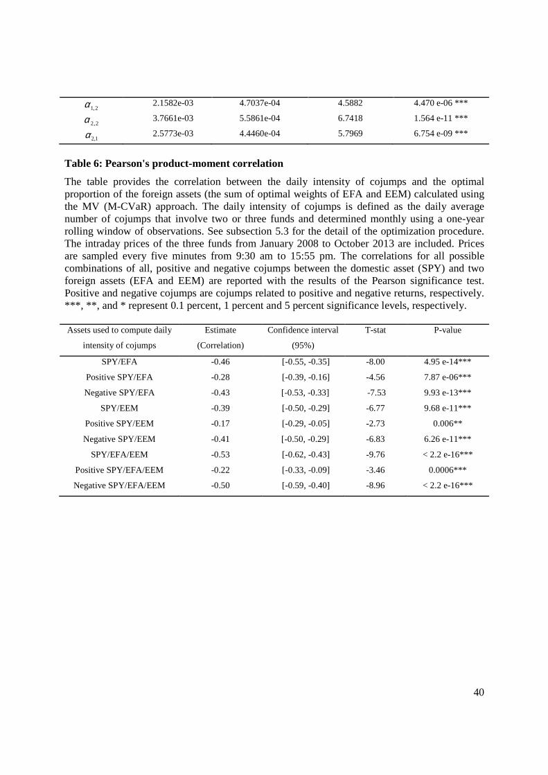
approach, summarized in Table 6,10 show a negative correlation between the demand of foreign

assets and the daily intensity of cojumps between the domestic market (SPY fund) and each of

foreign markets (EFA and EEM funds). We find a correlation of -0.46 for SPY/EFA cojumps

intensity and -0.39 for SPY/EEM cojumps intensity. When we consider the cojumps that involve

the three funds, we find a larger negative correlation (-0.53), which indicates that the holding of

foreign assets is more sensitive to the cojumps involving three funds than the cojumps between

two particular funds. Notably, the correlation coefficients are negative and larger for negative

cojumps than for positive cojumps, whatever the number of markets in the composite portfolio.

The sensitivity of foreign asset holding to number of cojumps is higher for the portfolio of SPY

and EFA funds than for the portfolio of SPY and EEM funds. This is expected given that the US

market have a very high correlation with the other developed ones. Finally, the proportion of

foreign assets is the lowest when jumps in three markets occur simultaneously. We also test the

significance of the Pearson correlation and find that the null hypothesis of no correlation is

statistically rejected for positive, negative and all market cojumps. This result confirms that the

negative link between the number of cross-market cojumps and the demand for the foreign assets

in international portfolios is economically meaningful. Similarly, we measure the correlation

between the daily intensity of idiosyncratic jumps (of respectively SPY, EFA and EEM funds)

and the optimal proportion of foreign assets and find that the correlation is not statistically

significant different from zero. For a sake of brevity, we do not tabulate this result in the paper. It

is available upon request. This result suggests that idiosyncratic jumps don’t affect the demand

for the foreign assets in international portfolios.

10 The results of the M-CVaR approach are not presented because MV and M-CVaR approaches lead to almost the same optimal portfolio composition. They are however available upon request.

24

*** Insert Table 6 here ***

*** Insert Table 7 here ***

We check the robustness of the correlation result by performing a regression analysis

where the optimal holding of foreign assets is explained by the number of cojumps. The results

presented in Table 7 show an estimated slope coefficient of -1.81 (-1.61 and -2.59) associated

with the daily intensity of cojumps between SPY and EFA funds (SPY/EEM funds and

SPY/EFA/EMM funds). All these coefficients are statistically significant at the 1% level. Thus,

if the average daily intensity of cojumps between SPY and EFA funds increases by 1%, the

optimal proportion of the foreign assets will decrease by -1.81%. The cojumps involving the

three funds have a greater effect as an increase of 1% in the daily intensity of cojumps of three

funds leads to a reduction of -2.59% of the proportion of foreign assets in the portfolio.

5.4 Cojumps and the benefits of international portfolio diversification

The results of the subsection 5.3 show that cojumps in international equity markets are an

indirect barrier to the holding of foreign assets. To the extent that they amplify the level of equity

market comovement, it is expected that they negatively affect the benefits of portfolio

diversification. We address this issue by looking at the link between the number of cojumps and

the measure of international diversification benefits in the spirit of Christoffersen et al. (2012),

which is calculated for the portfolio composed of three funds (SPY, EFA and EEM). Indeed,

Christoffersen et al. (2012) propose to measure the conditional diversification benefit (CDB) as

follows:

(23) ( ) ( )( )w

CDB ww

β ββ

β β

φ φφ α

−=

−

25

where and ( )wβφ are the values of the VaR and the CVaR of the portfolio loss function

associated with the vector of weights w and the confidence level .11 By construction, the

refers to the lower bound of the portfolio’s expected shortfall, while is the upper

bound of the portfolio’s expected shortfall and is defined as the weighted average of the

individual assets’ CVaRs ( ):

(24)

Thus, the CDB measure is a positive function with values ranging between 0 and 1, and

increases with the level of diversification benefit. Furthermore, it does not depend on the

expected returns and takes into account the nonlinearity of asset returns and the potential of their

nonlinear dependence (i.e., jumps, cojumps, and extreme movements).12

We calculate the monthly value of the CDB for our portfolio of three exchange-traded

funds based on the intraday data from the previous month (about 1617 intraday returns for each

fund per month). The confidence level is set at 5%. The weights allocated to three funds are

chosen monthly in a way to maximize the CDB. Figure 6 depicts the variation of the optimal

level of the CDB for the portfolio composed of three funds SPY, EFA and EEM. The CDB

measure fluctuates between 0.06 (August 2011) and 0.3 (August 2008 and January 2013). It is

high at the beginning and the end of the study period and relatively low during the global

financial crisis.

*** Insert Figure 6 here ***

11 See Appendix B for more details about the VaR and the CVaR of the portfolio loss function. 12 The high correlation of large down moves in international markets is documented by Longin and Solnik (2001) and Ang and Bekaert (2002).

( )wβα

β

( )wβα βφ

,iβφ

,1

n

i ii

wβ βφ φ=

=∑

β

26

To assess the effects of jumps and cojumps on the diversification benefit, we compute the

correlation between the optimal level of the CDB and the daily intensity of systematic and

idiosyncratic jumps, both calculated on a monthly basis from the cojumps and jumps detected

from the previous month. The daily intensity of cojumps refers to the daily average number of

cojumps involving three funds, while the daily intensity of idiosyncratic jumps refers to the daily

average number of jumps involving only one fund. We also consider the correlation between the

optimal level of CDB and a jump correlation measure. The latter is the monthly average

correlation of three funds, computed from the previous month intraday data. The jump

correlation of two particular funds takes into account both systematic and idiosyncratic jumps,

and is given by13:

(25)

where and are the intraday return of funds i and j, respectively over the

intraday time interval, m is the number of observations per one time unit, and

.

Obviously, the jump correlation increases with the number of systematic cojumps and decreases

with idiosyncratic jumps.

*** Insert Figure 7 here ***

*** Insert Table 8 here ***

13 See Jacod and Todorov (2009) for more details.

2 2, ,

1,

4 4, ,

1 1

mT

i j

i j mT mT

i j

p p

p p

τ ττ

τ ττ τ

ρ =

= =

∆ ∆=

∆ ∆

∑

∑ ∑

,ip τ∆ ,jp τ∆1

,m m

τ τ−

1,...,mTτ =

, 1, ,

ii i

m m

p p pτ τ τ −∆ = −

27

The findings in Table 8 show that the CDB is negatively correlated with the daily

intensity of systematic cojumps (-0.37) and with the jump correlation (-0.65). By contrast, the

CDB is positively correlated with the intensity of idiosyncratic jumps (0.4). The strong

dependence between the diversification benefit and the correlation of jumps is also shown in

Figure 7. Taken together, these results indicate that the international diversification benefit

increases with the intensity of idiosyncratic jumps and decreases with the level of systematic

cojumps observed in the international markets. They further confirm our previous findings that

domestic (US) investors will allocate more money towards home assets in the presence of

cojumps between domestic and foreign markets.

6 Conclusions

In this paper, we investigate how jumps and cojumps in international equity markets affect

international asset allocation and diversification benefits. Using a nonparametric intraday jump

detection technique developed by Lee and Mykland (2008) and Anderson et al. (2007) and

intraday data from three international exchange-traded funds as proxies for international equity

markets, we find that intraday jumps are transmitted both in time (in the same market) and in

space (across markets). The markets under consideration also have tendency to be involved in

systematic cojumps. The high and significant degree of jumps synchronization in international

equity markets suggests that the jump risk is rather systematic and thus could not be eliminated

through the diversification.

When studying the effects of cojumps on optimal international portfolio based on the MV

and M-CVaR approaches, we find evidence of a negative link between the demand for foreign

assets and the intensity of cojumps between domestic and foreign markets. This result implies

28

that a domestic (US) investor will invest less in foreign markets when the number of cojumps

increases. Putting differently, the high intensity of cojumps increases the cross-market

comovement between markets, and therefore reduces the international diversification benefit and

leads investors to prefer home assets. This result is also confirmed by the negative link between

the intensity of cojumps and the conditional diversification benefit measure suggested by

Christoffersen et al. (2012).

This work opens interesting perspectives for future research. It would be of great interest

to broaden the scope of this study by including a larger number of international equity indices

and studying the impact of asset cojumps on the demand for foreign assets for a larger panel of

countries. It is also interesting to investigate whether the mechanisms of jumps transmission

studied in this paper are also valid for individual country markets.

29

References

Ait-Sahalia, Y., Cacho-Diaz, J., and Laeven, R., 2015. Modeling financial contagion using

mutually exciting jump processes, Journal of Financial Economics 117, 585-606.

Aït-Sahalia, Y. , Xiu, D., 2016. Increased correlation among asset classes: Are volatility or

jumps to blame, or both?, Forthcoming Journal of Econometrics.

Andersen, T.G, Bollerslev, T., and Dobrev, D., 2007. No-arbitrage semi-martingale restrictions

for continuous-time volatility models subject to leverage effects, jumps and i.i.d. noise:

Theory and testable distributional implications. Journal of Econometrics 138 (1), 125-180.

Andersen, T.G., Dobrev, D., and Schaumburg, E, 2012. Jump robust volatility estimation using

nearest neighbor truncation. Journal of Econometrics 169 (1), 74-93.

Ang, A., and Bekaert, G., 2002. International Asset Allocation with Regime Shifts, Review of

Financial Studies 15, 1137-1187.

Artzner, P., Delbaen, F., Eber, J.M., Heath, D., 1997. Thinking coherently. Risk 10, 68-71.

Artzner, P., Delbaen, F., Eber, J., and Heath, D., 1999. Coherent measures of risk, Mathematical

Finance 9, 203-228.

Bae, K.H., Karolyi, G.A., and Stulz, R., 2003. A new approach to measuring financial contagion.

Review of Financial Studies 16, 717-763.

Barndorff-Nielsen O. E. and Shephard, N., 2004. Power and bipower variation with stochastic

volatility and jumps. Journal of Financial Econometrics 2, 1-37.

Barndorff-Nielsen, O. E. and Shephard, N., 2006a. Econometrics of testing for jumps in financial

economics using bipower variation. Journal of Financial Econometrics 4, 1-30.

Barndorff-Nielsen OE, Shephard N. 2006b. Measuring the impact of jumps on multivariate price

processes using bipower covariation. Manuscript.

Basak, S. and Shapiro, A., 2001. Value-at-risk based risk management: Optimal policies and

asset prices. Review of Financial Studies 14, 371-405.

Bekaert, G., Erb, C., Harvey, C., Viskanta, T., 1998. The distributional characteristics of

emerging market returns and asset allocation. Journal of Portfolio Management 24 (2), 102-

116.

Bollerslev, T., Law, T. H., Tauchen, G., 2008. Risk, jumps, and diversification. Journal of

Econometrics 144 (1), 234-256.

30

Bormetti, G., Calcagnile, L.M., Treccani, M., Corsi, F., Marmi, S., Lillo, F., 2015. Modelling

systemic price cojumps with hawkes factor models. Quantitative Finance 15, 1137-1156.

Christensen, K., Oomen, R., and Podolskij, M., 2014. Fact or friction: Jumps at ultra high

frequency. Journal of Financial Economics 114 (3), 576-599.

Christoffersen, P., Errunza, V., Langlois, H., and Jacobs, K., 2012. Is the Potential for

International Diversification Disappearing? Review of Financial Studies 25, 3711-3751

Corsi, F., Pirino, D., and Reno, R., 2010. Threshold bipower variation and the impact of jumps

on volatility forecasting. Journal of Econometrics 159, 276-288.

Das, S., Uppal, R., 2004. Systemic Risk and International portfolio choice. Journal of Finance

59, 2809-2834.

Dumitru, A.M. and Urga, G., 2012. Identifying jumps in financial assets: A comparison between

nonparametric jump tests. Journal of Business & Economic Statistics 30 (2), 242-255.

Dungey, M., McKenzie, M., and Smith, V., 2009. Empirical evidence on jumps in the term

structure of the US treasury market. Journal of Empirical Finance 16 (3), 430-445.

Dungey, M., Hvozdyk, L., 2012. Cojumping: Evidence from the US Treasury bond and futures

markets. Journal of Banking and Finance 36, 1563-1575.

Gaivoronski, A.A. and Pflug, G., 1999. Finding optimal portfolios with constraints on Value at

Risk, in B. Green, ed., Proceedings of the Third International Stockholm Seminar on Risk

Behaviour and Risk Management, Stockholm University.

Guidolin M., and Ossola E., 2009. Do Jumps Matter in Emerging Market Portfolio Strategies?

Chapter in Financial Innovations in Emerging Markets (Gregoriou G. editor), Chapman Hall,

London, 148-184.

Guidolin, M. and Timmermann, A., 2008. International asset allocation under regime switching,

skew, and kurtosis preferences. Review of Financial Studies 21 (2), 889-935.

Gilder, D., Shackleton, M., and Taylor, S., 2012. Cojumps in Stock Prices: Empirical Evidence.

Journal of Banking and Finance 40, 443-459.

Gnabo, J., Hvozdyk, L., and Lahaye, J., 2014. System-wide tail comovements: A bootstrap test

for cojump identification on the S&P500, US bonds and currencies. Journal of International

Money and Finance 48, 147-174.

Harris, L., 1986. A transaction data study of weekly and intradaily patterns in stock returns.

Journal of Financial Economics 16, 99-117.

31

Hawkes, A.G., 1971. Spectra of some self-Exciting and mutually exciting point Processes.

Biometrika 58, 83-90.

Huang, X. and Tauchen, G., 2005. The relative contribution of jumps to total price variance.

Journal of Financial Econometrics 3 (4), 456-499.

Jacod, J., and Todorov, V., 2009. Testing for Common Arrivals of Jumps for Discretely

Observed Multidimensional Processes. The Annals of Statistics 37, 1792-1838.

Jiang G. J. and Oomen, R. C. A., 2008.Testing for jumps when asset prices are observed with

noise - A swap variance approach. Journal of Econometrics 144, 352-370.

Jondeau, E., and Rockinger, M., 2006.Optimal portfolio allocation under higher moments.

European Financial Management 12 (1), 29-55.

Krokhmal. P., Palmquist, J., and Uryasev., S., 2002. Portfolio optimization with conditional

Value-At-Risk objective and constraints. The Journal of Risk 4, 11-27.

Lahaye J., Laurent, S., and Neely, C.J., 2010. Jumps, cojumps and macro announcements.

Journal of Applied Econometrics 26, 893-921.

Lee S. S. and Mykland, P.A., 2008. Jumps in financial markets: A new nonparametric test and

jump dynamics. Review of Financial Studies 21, 2535-2563.

Longin, F., and Solnik B., 2001, Extreme Correlation of International Equity Markets. Journal of

Finance 56, 649-676.

Markowitz, H.M., 1952. Portfolio Selection. Journal of finance 7 (1), 77-91.

Merton, R., 1976. Option pricing when underlying stock returns are discontinuous. Journal of

Financial Economics 3, 125-144.

Ogata, Y., 1978. The asymptotic behaviour of maximum likelihood estimates for stationary point

processes. Annals of the Institute of Statistical Mathematics 30, 243-261.

Ozaki, T., 1979. Maximum likelihood estimation of Hawkes’ self-exciting point processes.

Annals of the Institute of Statistical Mathematics 31(1), 145-155.

Pflug, G. Ch. 2000. Some remarks on the value-at-risk and the conditional value-at- risk. In.

“Probabilistic Constrained Optimization: Methodology and Applications”, ed. S. Uryasev.

Kluwer Academic Publishers, 2000.

Podolskij, M., Ziggel, D., 2010. New tests for jumps in semimartingale models. Statistical

Inference for Stochastic Processes 13 (1), 15-41.

32

Pukthuanthong, K., and Roll, R., 2015. Internationally correlated jumps. Review of Asset Pricing

Studies 5, 92-111.

Rockafellar, R. T. and Uryasev, S., 2000. Optimization of Conditional Value-at-Risk. Journal of

Risk 2, 21-41.

Rockafellar, R. T. and Uryasev, S., 2002. Conditional Value-at-Risk for General Loss

Distributions. Journal of Banking and Finance 26 (7), 1443-1471

Wood, R, A., McInish, A., Thomas H., and Ord, K., 1985. An investigation of transaction data

for NYSE stocks. Journal of Finance 40, 723-741.

33

Appendix A: Intraday volatility pattern

It is widely documented (Wood et al. (1985) and Harris (1986)) that intraday returns show a

systematic seasonality over the trading day, also called the U-shaped pattern. The intraday

volatility is particularly higher at the open and the close of the trading than the rest of the day.

To minimize the effects of intraday volatility on our jump detection test we modify our

procedure by rescaling intraday returns with a volatility jump robust corrector introduced by

Bollerslev and al. (2008). The kth rescaled intraday return of day t is defined by:

,

,ˆt k

t kk

rr

ς=

where:

,1 ,22 11 1 11

2 2,1 ,2 , 1 , , 1 , 1 ,

1 1 2 1

T

t tt

T T M T

t t t l t l t l t M t Mt t l t

M r r

r r r r r r r

ς =−

− + −= = = =

=+ +

∑

∑ ∑∑ ∑

1 1

2 2, 1 , , 1

2 11 112 2

,1 ,2 , 1 , , 1 , 1 ,1 1 2 1

, 2,..., 1

T

t k t k t kt

k T T M T

t t t l t l t l t M t Mt t l t

M r r rk M

r r r r r r r

ς− +

=−

− + −= = = =

= = −+ +

∑

∑ ∑∑ ∑

, 1 ,2 1

1 112 2

,1 ,2 , 1 , , 1 , 1 ,1 1 2 1

T

t M t Mt

M T T M T

t t t l t l t l t M t Mt t l t

M r r

r r r r r r r

ς−

=−

− + −= = = =

=+ +

∑

∑ ∑∑ ∑

T is the total number of days considered in the study and M is the number of observations in a

day.

34

Appendix B: Mean-CVaR optimization problem

The CVaR optimization approach initially developed by Rockafellar and Uryasev (2000) can be

described as follows. We first define the loss function of a portfolio composed of n assets given

the vector of weights w and the random vector of asset returns r such as

The probability of not exceeding a threshold is given by:

where is the density function of the vector of returns. is a function of for a fixed

vector of weights w and represents the cumulative distribution function for the loss associated

with the vector of weights w.

The values of the VaR and the CVaR of the loss function associated with w and a

confidence level , and , can be then determined as:

Following Rockafellar and Uryasev (2000), we provide the expression using the

function defined as follows:

( )1

,n

i ii

f w r w r w r=

′= − = −∑

( ),f w r α

( )( ),

, ( ) f w r

w p r drα

α≤

Ψ = ∫

( )p r Ψ α

β ( )wβα ( )wβφ

( ) ( )( )min : ,w R wβα α α β= ∈ Ψ ≥

( ) ( ) ( )( ) ( )

( )1

,

1 ,f w r w

w f w r p r drβ

βα

φ β −

≥

= − ∫

( )wβφ

Fβ

( ) ( ) ( ) ( )1, 1 ,F w f w r p r drβ α α β α

+− = + − − ∫

35

where . Rockafellar and Uryasev (2000) show that is convex

and continuously differentiable as a function of . It is also related to the CVaR of the loss

function through .

Moreover, the authors prove that minimizing over all is equivalent to

minimizing over all , that is .

The expression of can be simplified by generating a random collection of the vector of

returns and approximated with as follows:

Replacing the loss function by its expression gives:

By introducing the auxiliary variable , the minimizing of is equivalent to the linear

equation:

subject to: , for i = 1,…,q

If we add the budget and the expected target return constraints, the mean-CVaR

optimization problem is given by:

[ ] ( )max ;0x x+ = ( ),F wβ α

α

( ) ( )( )min ,R

w F wβ βαφ α

∈=

( )wβφ nw R∈

( ),F wβ α ( ), nw R Rα ∈ × ( )( )

( ),

min min ,n nw R w R R

w F wβ βαφ α

∈ ∈ ×=

Fβ

( ) ( ) ( )( )1 2, ,..., qr r r

iu

( ) 1

1

1

q

ii

uq

αβ =

+− ∑

0iu ≥ ( ) 0iiu w r α′+ + ≥

36

subject to

( ),1

1min

1

q

ii

uqα ω

αβ =

+− ∑

( )

1, , 0, 1,...,

0, 0, 1,...,

k

ii i

e w w w k n

u u w r i q

µ µ

α

′ ′= = ≥ = ′≥ + + ≥ =

37

Table 1: Summary statistics of jump occurrences and jump sizes

The number of total, positive (percentage) and negative (percentage) detected jumps from the returns of the three ETFs including SPY, ETA, and EEM are reported. The mean, standard deviation, skewness and kurtosis of jump sizes are shown. The percentage of positive jumps and negative jumps from all jumps are reported in brackets next to the number of positive jumps and negative jumps, respectively. Jumps are detected using the LM-ABD procedure with a critical value . See subsection 2.1 for the detail of jump test statistics. The intraday prices of the three ETFs from January 2008 to October 2013 are included. Prices are sampled every five minutes from 9:30 am to 15:55 pm.

SPY EFA EEM

Intraday jumps 1119 1114 1024

Positive jumps 475 (42%) 495 (44%) 455 (44%)

Negative jumps 644 (58%) 619 (56%) 569 (56%)

Mean (jump return) -4.3e-04 -2.5e-04 -2.1e-04

Standard deviation 0.0048 0.0047 0.0058

Skewness -0.59 0.27 -0.006

Kurtosis 14.00 8.40 15.60

Table 2: Summary statistics of jump occurrences at day level

The number of days with no jumps, one jump, and two jumps up to more than 5 jumps of the price of the three ETFs (SPY, EFA and EEM) are reported. The last row shows the percentage of days with at least one jump. Jumps are detected using LM-ABD procedure with a critical value

. See subsection 2.1 for the detail of jump test statistics. The intraday prices of the three ETFs from January 2008 to October 2013 are included. Prices are sampled every five minutes from 9:30 am to 15:55 pm.

SPY EFA EEM

0 843 843 879

1 357 365 353

2 139 147 128

3 75 50 60

4 30 37 26

5 12 13 9

More than 5 12 13 13

At least one jump 42% 42% 40%

4=θ

4=θ

38

Table 3: Summary statistics of cojump occurrences

The number of total positive and negative detected co-jumps among ETFs including SPY and EFA (column 1), SPY and EEM (column 2), EFA and EEM (column 3) and SPY, EFA and EEM (column 4) are reported. The percentage of cojumps compared to the total number of detected jumps is shown in brackets next to intraday cojumps. Jumps are detected using the LM-ABD procedure with a critical value . See subsection 2.1 for the detail of jump test statistics and subsection 2.2 for cojump identification procedure. The intraday prices of the three ETFs from January 2008 to October 2013 are included. Prices are sampled every five minutes from 9:30 am to 15:55 pm.

SPY / EFA SPY/EEM EFA/EEM SPY/EFA/EEM

Intraday cojumps 585 (53%) 509 (50%) 458 (45%) 365 (36%)

Positive cojumps 242 203 193 144

Negative cojumps 343 306 265 221

Table 4: Summary statistics of cojump occurrences at day level

The number of days with no cojumps, one cojump, two cojumps up to more than four cojumps among ETFs including SPY and EFA in column 2, SPY and EEM in column 3, EFA and EEM in column 4, and SPY, EFA, and EEM in column 5 are reported. The last row shows the percentage of days with at least one cojump. Jumps are detected using the LM-ABD procedure with a critical value . See subsection 2.1 for the detail of jump test statistics and subsection 2.2 for cojump identification procedure. The intraday prices of the three funds are from January 2008 to October 2013. Prices are sampled every five minutes from 9:30 am to 15:55 pm.

SPY/EFA SPY/EEM EFA/EEM SPY/EFA/EEM

0 1071 1130 1147 1208

1 282 233 233 193

2 70 61 57 39

3 27 28 19 20

4 12 11 6 5

More than 4 3 5 6 3

At least one cojump 27% 23% 22% 18%

4=θ

4=θ

39

Table 5: Maximum likelihood estimation of the bivariate Hawkes model

The table below shows the results of the maximum likelihood estimation of the bivariate Hawkes model for pairs of ETFs including SPY/EFA (panel A), SPY/EEM (panel B) and EFA/EEM (panel C). See subsection 5.2 for the detail of Hawkes process. The intraday prices of the three funds from January 2008 to October 2013 are included. Prices are sampled every five minutes from 9:30 am to 15:55 pm. The values of the estimate, standard error, z- statistic and p-value are reported for each parameter of the bivariate model. ***, **, and * represent 0.1 percent, 1 percent and 5 percent significance levels, respectively. Panel A: SPY / EFA

Estimate Std. Error z value Pr(z)

1.6305e-03 6.4929e-05 25.1122 < 2.2 e-16***

1.5445e-03 6.4217e-05 24.0505 < 2.2 e-16 ***

4.2957e-02 5.2288e-03 8.2154 < 2.2 e-16 ***

1.9230e-02 1.6585e-03 11.5942 < 2.2 e-16 ***

1.2004e-02 1.8520e-03 6.4816 9.074 e-11 ***

1.7864e-03 5.5554e-04 3.2156 0.001302 **

3.7166e-03 4.9845e-04 7.4563 8.896 e-14 ***

2.4015e-03 4.6676e-04 5.1452 2.673 e-07 ***

Panel B: SPY/EEM

Estimate Std. Error z value Pr(z)

1.5452e-03 6.4580e-05 23.9268 < 2.2 e-16***

1.4443e-03 6.3741e-05 22.6583 < 2.2 e-16 ***

1.8364e-02 1.6053e-03 11.4395 < 2.2 e-16 ***

1.8342e-02 1.6588e-03 11.0573 < 2.2 e-16 ***

4.0540e-03 5.3480e-04 7.5804 3.445 e-14***

2.1598e-03 4.6120e-04 4.6829 2.828 e-06 ***

3.8814e-03 5.5318e-04 7.0164 2.277 e-12 ***

2.2278e-03 4.2694e-04 5.2181 1.808 e-07 ***

Panel C: EFA/EEM

Estimate Std. Error z value Pr(z)

1.5471e-03 6.2625e-05 24.7045 < 2.2 e-16***

1.4194e-03 6.2419e-05 22.7400 < 2.2 e-16 ***

2.6309e-02 2.7030e-03 9.7335 < 2.2 e-16 ***

2.5798e-02 2.7876e-03 9.2544 < 2.2 e-16 ***

4.0065e-03 5.2480e-04 7.6342 2.272 e-14 ***

∞,1λ

∞,2λ

1β2β1,1α

2,1α

2,2α

1,2α

∞,1λ

∞,2λ

1β2β1,1α

2,1α

2,2α

1,2α

∞,1λ

∞,2λ

1β2β1,1α

40

2.1582e-03 4.7037e-04 4.5882 4.470 e-06 ***

3.7661e-03 5.5861e-04 6.7418 1.564 e-11 ***

2.5773e-03 4.4460e-04 5.7969 6.754 e-09 ***

Table 6: Pearson's product-moment correlation

The table provides the correlation between the daily intensity of cojumps and the optimal proportion of the foreign assets (the sum of optimal weights of EFA and EEM) calculated using the MV (M-CVaR) approach. The daily intensity of cojumps is defined as the daily average number of cojumps that involve two or three funds and determined monthly using a one-year rolling window of observations. See subsection 5.3 for the detail of the optimization procedure. The intraday prices of the three funds from January 2008 to October 2013 are included. Prices are sampled every five minutes from 9:30 am to 15:55 pm. The correlations for all possible combinations of all, positive and negative cojumps between the domestic asset (SPY) and two foreign assets (EFA and EEM) are reported with the results of the Pearson significance test. Positive and negative cojumps are cojumps related to positive and negative returns, respectively. ***, **, and * represent 0.1 percent, 1 percent and 5 percent significance levels, respectively. Assets used to compute daily

intensity of cojumps

Estimate

(Correlation)

Confidence interval

(95%)

T-stat P-value

SPY/EFA

Positive SPY/EFA

Negative SPY/EFA

SPY/EEM

Positive SPY/EEM

Negative SPY/EEM

SPY/EFA/EEM

Positive SPY/EFA/EEM

Negative SPY/EFA/EEM

-0.46

-0.28

-0.43

-0.39

-0.17

-0.41

-0.53

-0.22

-0.50

[-0.55, -0.35]

[-0.39, -0.16]

[-0.53, -0.33]

[-0.50, -0.29]

[-0.29, -0.05]

[-0.50, -0.29]

[-0.62, -0.43]

[-0.33, -0.09]

[-0.59, -0.40]

-8.00

-4.56

-7.53

-6.77

-2.73

-6.83

-9.76

-3.46

-8.96

4.95 e-14***

7.87 e-06***

9.93 e-13***

9.68 e-11***

0.006**

6.26 e-11***

< 2.2 e-16***

0.0006***

< 2.2 e-16***

2,1α

2,2α

1,2α

41

Table 7: Linear regression

The optimal demand of the foreign assets in the studied portfolio is regressed on the number of cojumps. α and β are the intercept and slope of the OLS regression, respectively. The demand of foreign assets is defined as the sum of optimal allocation weights of EFA and EEM funds resulting from our portfolio optimization procedure based on weekly historical returns (294 observations for each fund) and the MV and M-CVaR approaches. The cojumps are between SPY and EFA, SPY and EEM, and SPY, EFA, and EEM. Jumps are detected using LM-ABD procedure with a critical value . See subsection 2.1 for the detail of jump test statistics. Cojumps are jumps occurring in two or three markets simultaneously. See subsection 2.2 for cojump identification procedure. The intraday prices of the three funds from January 2008 to October 2013 are included. Prices are sampled every five minutes from 9:30 am to 15:55 pm. Panels A, B, and C report the results for all, negative, and positive cojumps, respectively. ***, **, and * represent 0.1 percent, 1 percent and 5 percent significance levels, respectively. Panel A: All cojumps

All cojumps Coefficient Estimate St.dev T-stat P-value

SPY/EFA α 1.23 0.09 13.37 < 2.2 e-16***

β -1.81 0.22 -8.00 4.9 e-14***

SPY/EEM α 1.06 0.08 12.60 < 2.2 e-16***

β -1.61 0.23 -6.70 9.7 e-11***

SPY/EFA/EEM α 1.15 0.06 16.90 < 2.2 e-16***

β -2.59 0.26 -9.76 < 2.2 e-16***

Panel B: Negative cojumps

Panel C: Positive cojumps

Positive cojumps Coefficient Estimate St.dev T-stat P-value

SPY/EFA α 0.86 0.08 10.69 < 2 e-16***

β -2.21 0.48 -4.56 7.8 e-16***

SPY/EEM

α 0.73 0.08 8.37 4.3 e-15***

β -1.72 0.62 -2.73 0.006**

SPY/EFA/EEM α 0.77 0.08 9.65 2.5 e-16***

β -2.72 0.78 -3.45 0.0006***

4=θ

Negative cojumps Coefficient Estimate St.dev T-stat P-value

SPY/EFA α 1.07 0.07 13.92 < 2 e-16***

β -2.38 0.31 -7.53 9.9 e-13***

SPY/EEM α 0.92 0.06 14.54 < 2 e-16***

β -2.00 0.29 -6.84 6.2 e-11***

SPY/EFA/EEM α 0.91 0.04 18.95 < 2 e-16***

β -2.73 0.30 -8.96 < 2 e-16***

42

Table 8: The impact of cojumps on the optimal level of the diversification benefit

The table reports the measures of correlation between the optimal level of the diversification benefit and the correlation of jumps, the daily intensity of cojumps and idiosyncratic jumps, respectively with the results of the Pearson significance test. The diversification benefit is defined in subsection 5.4. The correlation of jumps is the average value of the correlation of jumps among the three ETFs including SPY, EFA, and EEM calculated on a monthly basis. The LM-ABD is applied to detect jumps. See subsection 2.1 for the detail of jump test statistics and subsection 2.2 for cojump identification procedure. The daily intensity of cojumps is computed on a monthly basis as the daily average number of cojumps that involve three funds detected from the previous month. The daily intensity of idiosyncratic jumps is measured on a monthly basis as the daily average number of jumps that involve only one market. The intraday prices of the three funds from January 2008 to October 2013 are included. Prices are sampled every five minutes from 9:30 am to 15:55 pm.

The measure used to compute the correlation with the optimal level of

the diversification benefit

Estimate (Correlation)

Confidence interval (95%)

T-stat P-value

Correlation of jumps -0.65 [-0.77, -0.49] -7.05 1.1 e-09***

Intensity of cojumps -0.37 [-0.56, -0.15] -3.3 0.0015**

Intensity of idiosyncratic jumps 0.40 [0.18, 0.58] 3.61 0.0005***

43

Figure 1 : Volatity pattern corrector

This figure shows the variation of the volatility pattern corrector during the trading hours (from 9:30 am to 15:55 pm, UTC−4). The intraday volatility is high at the opening and the closing of the market with a remarkable jump around 10:00 am, which corresponds to the usual time of macroeconomic announcements. See Appendix A for the detailed description of the volatility jump robust corrector. The intraday prices of the three ETFs including SPY, EFA, and EEM from January 2008 to October 2013 are included. Prices are sampled every five minutes from 9:30 am to 15:55 pm.

44

45

Figures 2 and 3: Jump and cojump occurences

These figures show the variation of the daily jump and cojump intensities of the three funds (SPY, EFA, and EEM) from January 2008 to October 2013. The daily intensity of jumps (cojumps) is defined as the daily average number of jumps (cojumps that involve two or three funds). These time-varying jump intensities are calculated daily using a rolling six-month window of observations. Prices are sampled every five minutes from 9:30 am to 15:55 pm. Jumps are detected using the LM-ABD procedure with a critical value . See subsection 2.1 for the detail of jump test statistics and subsection 2.2 for cojump identification procedure.

4=θ

0.00

0.20

0.40

0.60

0.80

1.00

1.20

Jul-0

8

Oct

-08

Jan-

09

Ap

r-0

9

Jul-0

9

Oct

-09

Jan-

10

Ap

r-1

0

Jul-1

0

Oct

-10

Jan-

11

Ap

r-1

1

Jul-1

1

Oct

-11

Jan-

12

Ap

r-1

2

Jul-1

2

Oct

-12

Jan-

13

Ap

r-1

3

Jul-1

3

Oct

-13

Daily jump intensity

SPY EFA EEM

0.00

0.10

0.20

0.30

0.40

0.50

0.60

0.70

Jul-0

8

Oct

-08

Jan-

09

Ap

r-0

9

Jul-0

9

Oct

-09

Jan-

10

Ap

r-1

0

Jul-1

0

Oct

-10

Jan-

11

Ap

r-1

1

Jul-1

1

Oct

-11

Jan-

12

Ap

r-1

2

Jul-1

2

Oct

-12

Jan-

13

Ap

r-1

3

Jul-1

3

Oct

-13

Daily cojump intensity

SPY_ EFA SPY_EEM EFA_EEM SPY_EFA_EEM

46

Figure 4: Time and space clustering of intraday jumps

This figure shows the arrival times of intraday jumps of the three funds from April 2010 (574th day of the sample) to November 2010 (715th day of the sample). The intraday prices of the three ETFs including SPY, EFA, and EEM are included. Prices are sampled every five minutes from 9:30 am to 15:55 pm.

Figure 5 : The variation of the optimal proportion of foreign assets

Panel A shows the variation of the optimal proportion of the foreign assets (EFA and EEM) from MV and M-CVaR approaches. The optimal portfolio composition is determined in a monthly basis, using a one-year rolling window of weekly returns. The portfolio is composed of one domestic asset (SPY) and two foreign assets (EFA and EEM). Panel B and C presents moving standard deviation and absolute value of the CVaR, respectively of SPY, EFA and EEM. These variations are obtained for a rolling six-month window of daily returns. The intraday prices of the three ETFs including SPY, EFA, and EEM from January 2008 to October 2013 are included. Prices are sampled every five minutes from 9:30 am to 15:55 pm. Panel A: Optimal demand of foreign assets under MV and M-CVaR

47

Panel B: Standard deviation of SPY, EFA and EEM

0

0.2

0.4

0.6

0.8

1

1.2Ja

n-09

Apr

-09

Jul-

09

Oct

-09

Jan-

10

Apr

-10

Jul-

10

Oct

-10

Jan-

11

Apr

-11

Jul-

11

Oct

-11

Jan-

12

Apr

-12

Jul-

12

Oct

-12

Jan-

13

Apr

-13

Jul-

13

Oct

-13

Optimal demand of foreign assets (EFA+EEM)

MV CVAR

0

0.01

0.02

0.03

0.04

0.05

0.06

0.07

Jul-

08

Oct

-08

Jan-

09

Apr

-09

Jul-

09

Oct

-09

Jan-

10

Apr

-10

Jul-

10

Oct

-10

Jan-

11

Apr

-11

Jul-

11

Oct

-11

Jan-

12

Apr

-12

Jul-

12

Oct

-12

Jan-

13

Apr

-13

Jul-

13

Oct

-13

Standard deviation

SPY EFA EEM

48

Panel C: CVaR of SPY, EFA and EEM

Figure 6: The conditional diversification benefit (CDB)

The figure shows the variation of the optimal level of the diversification benefit calculated monthly based on an international portfolio composed of three funds SPY, EFA and EEM. See subsection 5.4 for the definition of conditional diversification benefit. The intraday prices of the three funds from January 2008 to October 2013 are included. Prices are sampled every five minutes from 9:30 am to 15:55 pm.

0

0.02

0.04

0.06

0.08

0.1

0.12

0.14

Jul-0

8

Oct

-08

Jan-

09

Ap

r-09

Jul-0

9

Oct

-09

Jan-

10

Ap

r-10

Jul-1

0

Oct

-10

Jan-

11

Ap

r-11

Jul-1

1

Oct

-11

Jan-

12

Ap

r-12

Jul-1

2

Oct

-12

Jan-

13

Ap

r-13

Jul-1

3

Oct

-13

CVaR

SPY EFA EEM

0.00

0.05

0.10

0.15

0.20

0.25

0.30

0.35

Jan-

08

Ap

r-0

8

Jul-0

8

Oct

-08

Jan-

09

Ap

r-0

9

Jul-0

9

Oct

-09

Jan-

10

Ap

r-1

0

Jul-1

0

Oct

-10

Jan-

11

Ap

r-1

1

Jul-1

1

Oct

-11

Jan-

12

Ap

r-1

2

Jul-1

2

Oct

-12

Jan-

13

Ap

r-1

3

Jul-1

3

Oct

-13

CDB

49

Figure 7: Linear regression between the conditional diversification benefit (CDB) and the correlation of jumps

The figure displays a scatterplot with a regression line showing the linear relationship between the optimal level of the conditional diversification benefit and the level of the correlation between jumps. Diversification benefit is defined in subsection 5.4. The correlation of jumps is the average value of the correlation of jumps from different pairs of the three ETFs including SPY, EFA, and EEM on a monthly basis. The LM-ABD is applied to detect jumps. See subsection 2.1 for the detail of jump test statistics. The intraday prices of the three funds from January 2008 to October 2013 are included. Prices are sampled every five minutes from 9:30 am to 15:55 pm.