PAPER P-853

INTERNAL WAVE-SURFACE WAVEINTERACTIONS REVISITED

F. Zachariasen

DF)C-

March 1972 1j A29 1912

C

;ll UNA !. rcICHNICALINFORMATION SERVICE

',~,tj bttVA 2,'1i1

SINSTITUTE FOR DEFENSE ANALYSESL..JD JASON

IDA Log No. HQ 72-1418-Copy •4 of 70 coph

.l~ ...... ........ .lyS I... .......... •. .

31 ..............-•.......1ItTItII•I0I/AVAI'" !'.lfY C03ES

118t. LZAf L.x SP&CIAL

The work reported in this document was conducted under contractDAHC15 67 C 0011 for the Department of Defense. The publicationof this IDA Paper does not indicate endorsement by the Departmentof Defense, nor should the contents be construed as reflecting theofficial position of that agency.

.d

SApproved for public release; distribution unlimited. I

.1

-j

I.!

~ 7 l

UNCLASSIFIED

Sevunty ClawBfictiBon

DOCUMENT CONTROL DATA - R At P£S&Corya ssi.eD s I.. tefio *1 toml. 60dr of .hstre.t &ad Jeessule mrwitattanmus ovo e wed .Aha the .ohr.II tepos is assll,*d)

I mGa N .G.... ACYIVITY ICoe. . L

INSTITUTE FOR DEFEN&m ANALYSES 1:0NcLiASSIFIED

400 Army-Navy Drive GROUP

Arlington, Virginia 22202 --

Internal Wave-Surface Wave Interactions Revisited

4 oescoliploveNOE .015 t "D of eP- aed #"#weirse d'os )

Paper P-853, March 1972S AU t"O"ICs (ffire nsme. middle Iiti5al. .3met.OJ

F. Zachariasen

* M1,OMT OATS[ ?Pa. TOTAL NO OF PA9I8 6b. No or NaraMarch 1972 21 0

&A CONTRAC T ON GRANT ?40 NO. OMIOINATON? S REPORT NUM-1iEWIR

DAHCI5 67 C 0011 P853

JASON€b. OTVNON M*&PO NOISI (AM, elaMt.M4mhtO -ft SO ... Ipo.d

d None.6 O.ST"01SJON STATEMENT

Approved for public release; distribution unlimited.

t"NART NOTES 1 9 SPONIOVING UILITVAMV ACTIViT,

- Defense Advanced Research Proj-None ects Agency

lArlinton, Virginia 22209S, .USTPAC T

The interaction of internal waves and surface waves in

water is explored in the regions where the effects of the inter-

action are small. Explicit- solutions for an arbitrary internal

wave are given for various kinds of boundary conditions, with a

detailed discussion of the conditions under which they are valid.

The connection of the solutions with the conservation equations

is made explicit, and the modifications produced by viscous

damping are outlined.

S/10,

DD , '.. 1473 UNCLASSIFIEDDD INov G 147,Secu3.V CIiimlfiCmtOHIC

UNCLASSIFIED------ G untY Classification--

*@L59 WT *OL49 WT MOLS .1

F Interxnal water wavesI Perturbation of surface waves

Viscous damping

g-awilty classificationI

PAPER P-853

"INTERNAL WAVE-SURFACE WAVE

INTERACTIONS REVISITED

F. Zachariasen

March 1972 DrCn f CJ. AG29 19?Z t

IDAINSTITUTE FOR DEFENSE ANALYSES

JASON

400 Army-Navy Drivc, Arlington. Virginia 22202

Contract DAHC15 67 C 0011

7.

ABSTRACT

The interaction of internal waves and surface waves in

water is explored in the regions where the effects of the

interaction are small. Explicit solutions for an arbitrary

internal wave are given for various kinds of boundary con-ditions, with a detailed discussion of the conditions under

which they are valid. The connection of the solutions with

the conservation equations is made explicit, and the modifi-

cations produced by viscous damping are outlined.

S~ii

CONTENTS

"I. Introduction 1

"II. Basic Equations 5

III. Perturbation Solution 8

IV. Conservation Equations 13

V. Properties of the Solutions 16

VI. Other Boundary Conditions 18

"VII. Viscous Damping 21

o111

I. INTRODUCTION

This paper is to be viewed as a sequel to an earlier work

on the internal wave-surface wave interaction in water, which

appeared in IDA/JASON Study S-334.* We wish to enlarge on the

previous analysis in the following ways:

1. Clarify the assumptions involved in the calculation.

2. Correct the result in (I) by including a term which

was unjustifiably neglected.

3. Extend the solution to ranges of the parameters not

treated in (I).

4. Establish the connection with the approach to the

problem based on the conservation equations, and

5. Include the effect of viscous damping of the surface

waves.

Let us begin with a brief recapitulation of the problem

which we wish to discuss. We assume the existence originally

of a surface wave, that is, of a displacement of the surface

of an infinite ocean, given by ho(xt) = A exp i(kox - wot)

with Wo= An internal wave with velocity U--which is

The complete reference is IDA/JASON Study S-334, Generationand Airborne Detection of Internal Waves from an Object MovingThrough a Stratifie: Ocean, JASON 1968 summer study, Vol. II,

April 1969, p. 69. We shall refer to this as (I) in what*follows.

We shall, for simplicity, assume there is only one horizontaldimension (denoted x). The depth variable is called z, andis measured positive up. We are also going to confine our-selves to gravity waves--hence (since the water is assumedto be infinitely deep) we take wo /go" This limits us tovalues of 1; < 3 cm "1. T

'_IOU,

a.;sumed to be s given, but arbitrary, function of space andtime--is turned on, and this produces, for later times, achange 6h(x,t) in the surface displacement. The problem is tocalLr!iaý -- 6h.

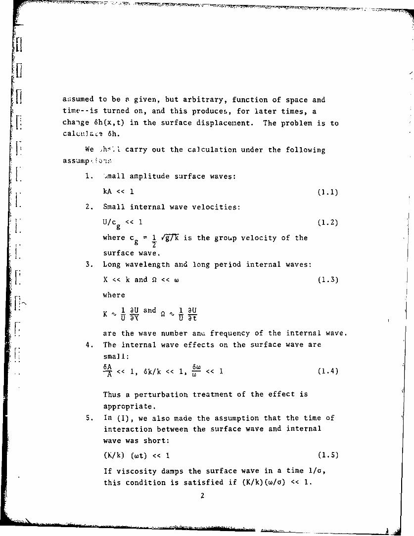
P We hr, * carry out the calculation under the followingassumnp -

1. ',mall amplitude surface waves:

kA< (1.1<)

2. Small internal wave velocities:

U/c << 1 (1.2)

where cg = 1 /g7/ is the group velocity of the

surface wave.3. Long wavelength and long period internal waves:

X << k and Q << w(13

where

K %,1 3U and a UK U a U at

V' are the wave number anu frequency of the internal wave.4. The internal wave effects on the surface wave are

small:6A ý_w

<< 1, 6k/k << 1, W << 1 (1.4)

Thus a perturbation treatment of the effect is

appropriate.

5. In (I), we also made the assumption that the time ofinteraction between the surface wave and internal

wave was short:

(K/k) (wt) << 1 (1.5)

If viscosity damps the surface wave in a time 1/a,

this condition is satisfied if (K/k)(w/a) << 1.

S2•.

Assumption (5) was mAde for convenience in (I), but was

not essential to the t.'.ýat.Aept. We shall therefore, here,I also obtain th.e solution without imposing this constraint. Weshall, however, s:ill fiind it useful in practice to keep a

weaker limit on the 'ime, namely (K/k) 4 (wt) 2 < 1; to relax

this requirement too is possible, but prevents us from exhibit-

ing the solution in a very explicit form.

A typical set of numbers with which we may be concerned

is as follows:

k = 1icm'1

A= 0.1 cm

U =1 cm/sec

K= I0- cm'

C = 1c cm/sec

For k = 1 cm 1, we have a = 3x10 '/sec, cg = 15 cm/sec and

w = 30 sec

With these parameters all of our conditions would appear

to be met: we have

kA = 0.1U/cg = 0.07

K/k = 10

Q/W = SxlO1

(K/k) - w/o = 0.1

The question of how well this idealized problem imitates

the real ocean is of course a serious one. Probably the mostimportant physical effect that has been ignored entirely is

wind. We have pretended that the wind enters only indirectly,

in that it is responsible for the generation of the surface

waves, but that once generated, the surface wave is no longer

seriously influenced by the wind and is merely eroded by

3

id

viscosity in some finite distance--or time--depending on itswavelength. This is evidently a great idealization.

The next most serious difficulty would appear to be in

the validity of the kA << I assumption. Nonlinear effects iiithe surface wave amplitude may well become important as SA/Aincreases from zero, and invalidate the treatment given hereeven when 6A/A is still quite small.

.14

-t

• 4

__ _ _

Ii

II. BASIC EQUATIONS

To obtain our basic equations we first write the equations

for a free surface:

W9 T -wi = WEy

both evaluated at z = . The notation is obvious: I is the

surface displacement and j is the velocity potential. We have,

in addition

and the boundary condition that 4 • €, where as

z - -. 4 is assumed to be a given function, and represents

the velocity potential of the internal wave.

The next step is to expand the surface equations to second

order in I. Then we write

E= h + H

•=4'=+4

and keep all first-order term; in either h or P. We choose H

and 4' (which are of course to be identified with the internal

wave) to satisfy the free surface equations by themselves (to

frist orler in H--and we furthermore assume that the z-depend-

ence in the internal wave is weak.) We then obtain equations

for h and 0, viz:

3h + U 2h + h N •4 _ (2.1)-Y -ax ax az gax at

5

Ss JSk~

(2.2)T- + IJ 7_ = -gh

evaluated at z = 0, together with

V20 = 0

and the boundary condition 0 - 0 as z ÷ - •. The symbol U

stands for the x component of the internal wave velocity 0.

We have thus far made use of assumption 1.1, the small

amplitude assumption.

Equations 2.1 and 2.2 are our starting point; comparing

with (I) we note the presence in Eq. 2.1 of the term h aU/ax.

"In (I) this was neglected in accord with assumption 1.3 with

the argument that it was small compared to U ah/ax. in mag-

- .. nitude, this is true; but the two terms are of different phase,

and hence it is not legitimate to ignore h aU/ax. This fact

will become more transparent later.

The next convenient thing to do is to eliminate 0 between

Eqs. 2.1 and 2.2 to obtain an equation for h alone, which is,

after all, the quantity of primary interest. This is made

feasible through V24 =0 and the fact that 0 ÷ 0 as z D -,

which permits us to writedk teikx Iklz4)(x,z,t) = f ZT O(k,t) eke

Hence (we take k positive) we have

3. 0/az = -i a4/ax (2.3)

We can now get rid of 0. Equations 2.1 and 2.2, together with

assumptions 1.2 and 1.3, yield

- ig h = -2U _2_h - 2 DU ah - 2 M 3h (2.4)

We have neglected all quadratic terms in U, and all second and

6

I-~.. higher derivatives of U, in obtaining this result. The

boundary condition which we associate with Eq. 2.4 is that fort > 0, h = h (xt), some specified surface wave present before

0

the internal wave was turned on. Normally, we shall take h0"" ~to be simply

ho = A ei(koX-Wot) (2.5)

where|=

* 1

Wo 7

I 7

!7

"III. PERTURBATION SOLUTION

We assume that the effect of the internal wave on the

surface wave which was present initially will be small (As-

sumption 1.4). We may then write

h = h + 6h, h >> 6h (3.1)

where, to first order in the perturbation,

(2 a 0•uho DU ho aU Mho"3_ - ig 27 h = -2U TX-9 - 2 T-t Tx 2 •-•x

"for the simple choice (2.5), this simplifies to

--- ig 6h = (-2k00 U + 2iw 2- - 2ik 2-U]h

"- Z(x,t) h0 (x,t) (3.2)

This will be recognized as the same equation as that used in

(I) except that the coefficient of WU/ax in (I) was iwo rather

than 2iwo. The factor of 2 reflects the existence of the

h alU/ax term in Eq. 2.1.

It may be objected that the derivation of Eq. 3.2 is in-

valid, since it relied on the assumption that ho >> 6h, and

for certain values of x and t (for which ho vanishes) this in-

equality is false. However, these values constitute a very

small range of x and t, and do not, in fact, affect the cor-

rectness of Eq. 3.2. This will be made explicit in Section IV,

8

S~where we will obtain the same result without use of the as-

. ~sumption that h° >> 6h.

I In any event, our problem is now a straightforward one,-namely to solve Eq. 3.2 with the boundary condition that

6h = 0 for t < 0. This can be re directly by the method used

in (I). Let A be the retarded Green's function, so that

1W - ig A =6(x) 6(t) (3.3)

with A = 0 for t < 0.

Then

6h(x,t) = ff dx'dt' A(x-x',t-t') Z(x',t') ho(x',t')

and using the (obvious) solution to Eq. 3.3 together with

Eq. 2.5, we find

6h(x,t) C dO dk eikx f' dw e-id(t-t')ho(x,t f dt' f Z(kt') e -fx gk-2•OWO W, (3.4)

whereCO

Z(k,t) E f dx e-ikx Z(x,t)

The integral over dw in Eq. 3.4 is to be taken above the poles

of the denominator in the complex w plane because A is the re-

tarded Green's function.

Up to this point we have invoked assumptions 1.1, 1.2,1.3 and 1.4 but have made no use of 1.5. Equation 3.4 con-

stitutes a complete solution to the problem; however for a

given (arbitrary) U some numerical integrations will be re-quired to obtain a solution. It is therefore of some interest

to try to simplify 3.4.

9

'I

To do this we note that from assumption 1.3, U, and henceZ, may be expected to have only small frequency components

present. Hence we may expect w to be small, so we may expandV" the denominator in Eq. 3.4:

1 = + + ... (3.5)

gk-2ww0 -w2 gk-2ww0 (gk-2ww 0 ) 2

The first term in this expansion, after evaluation of the con-

tour integral over dw, yields directly

6h _ i t11 Tw-2• f- dr' Z(x - cg9(t-t'), t') (3.6)

0 0 -CO

S""Let us assess the error involved in stopping at this point.

-A To do this it is important to note that, from Eq. 3.2, Re Z is

bigger than Im Z by a factor "' k/K. Since the next term in

the expansion is out of phase by 900 with this term, the first

term alone will be an excellent approximation to Im 6h/h 0 buta less good one for Re 6h/h . In fact the errors are evidently

of order (w 0 t) (K/ko )3 and (w 0 t) (K/k 0 ) for the imaginary and

-•real parts, respectively.

The first term is thus a good approximation for the real

I part of 6h/h 0 ; that is, for 6A/Ao, if the "short time assump-

tion," 1.5, is valid. It is a good approximation for the

" I imaginary part, that is for 6w and 6k, in any event.

In the case of short wavelength internal waves, or long

Sj wavelength surface waves, where assumption 1.5 may not be

satisfied, we may keep the next term in the expansion 3.5.

This leads to the result

I3 10

6h i t6h 2•o-F z(x c (t-t'), t') dt'

+ f t (t-t) a Z(x,)t-t') dt' (3.7)4Wo2 -00 at t2 x =X-cg9(tt

We may again estimate the error involved in stopping here,

and because of the alteration in phase by 900 of successive

terms in the expansion, it is clear that this is now an ex-

cellent approximation for both real and imaginary parts.

The successive terms are of the following magnitudes:

Imaginary part:

Real part: [(K + + (2 (0)o + (t.o']

Thus the neglected terms are of order (wot) 2 (•/wo) 4 in both

cases.

Finally, we may extract from Eq. .7 expressions for6A/Ao and 6k/ko, the quantities of real interest. We find,

using the definition of Z,

Ik_ U(x _ cx (t-t'), t') dt' (3.8)

and

6A U t U(x c (t-t'), t') dt'A 4c 9-' - CO ý ux - 9 ,-:• :)•:4c t

f O t-, U(x -c 9(t-t'), t') dt' (3.9)-~ ax2

The last term in 3.9 may be dropped if the short time assump-

tion is valid; we have neglected the corresponding term in

6k/ko in any event,

Comparing 3.8 and 3.9 with the results given in (I), wenote that the expression for 6k is the same, but that for6A differs by factors of 2 (apart from the a 2U/;x 2 term); these

changes are caused by the h DU/3x term in the original equation

with which we began.

12

IV. CONSERVATION EQUATIONS

We now return to our starting point, Eq. 2.4. Instead of

making a perturbation expansion of this immediately, as we didin Section III, let us use it to derive equations for the ampli-

tude, wave number and frequency directly. This is easily

done with the following definitions:

h = AeiX (4.1)

k = 3X/3x (4.2)

W= -ax/at (4.3)

The definitions 4.2 and 4.3 lead immediately to the so-called"conservation of waves":

3k +w . 0 (4.4)

We substitute 4.1 to 4.3 into 2.4, and separate 2.4 intoreal and imaginary parts, and find after a small amount ofalgebraic juggling that

2 _ 1gk - A -2kw U

3U 1 aA 2U 1 aA+ 2 i.,.+ 2 •

+ 2U a2 A (4.5)

13

and

.. (B •+ 3-N + 1 3w

"" kU A 1 3A U w

+k 3U 3U (4.6)W 7-1y - X-£

The first of these is the real part of 2.4, the second the

imaginary part.

These two equations are recognizable as the dispersion

relation and the conservation of energy, respectively. (One

should multiply the second through by A2 to make this obvious.)

Let us now introduce the perturbation expansion in U.

Thus we write A = A + 6A, k = k + 6k, w = w + 6w and assume000

6A << Ao, etc. The zero-order equations obviously tell us

that A = constw / and k= const. The first-order0 0oequations are

6w k U+c 6k (4.7)

+ c 1-) 6k -ko 'U (4.8)

:a- -6t x•A a •.Xk 3 +U 1 au (4.9)

0 0

where we define Cg g/2wo = (1/2) ='o'o

"We have used 4.4 to eliminate 6w in deriving these, and1- have also neglected higher derivatives of 6A.

First of all, these equations are immediately seen to"coincide with Eq. 3.2, thereby confirming the use of ho >> 6h,

in spite of the small range of x and t over which this may

14- ."4 9

not be true. Second, these coincide with the usual results

obtained from the conservation equations.*

Finally, the solutions may be written down by inspection,

(incorporating the boundary conditions that 6A and 6k vanish

when t < 0) and are seen to coincide exactly with Eqs. 3.8 and

3.9. The fact that the solutions to 4.8 and 4.9 agree exactly

with 3.8 and 3.9, which are only the first two terms in the

expansion of the solution Eq. 3.4 to 3.2, stems from theneglect of higher derivatives of 6A in deriving 4.8 and 4.9.This observation should help to clarify what is being dropped

when higher terms in the expansion 3.5 are neglected.

0. M. Phi!.ips, Dynamics of the U2per Ocean, Cambridge, 1966,p. 50. Noce that we have an additional term in aU/at not"given by Phillips. Presumably he omits this because of thetime averaging he uses to obtain the conservation equations.

i15

11

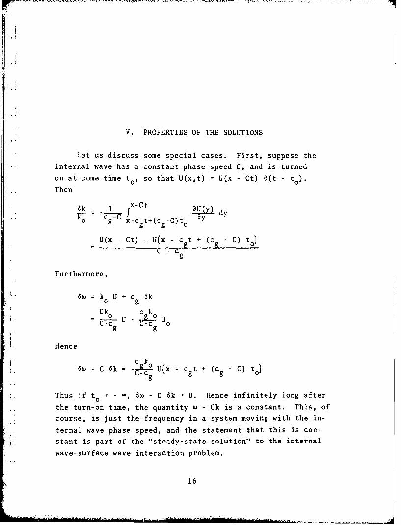
V. PROPERTIES OF THE SOLUTIONS

'ct us discuss some special cases. First, suppose the

internal wave has a constant phase speed C, and is turned

on at some time to, so that U(x,t) = U(x - Ct) 9(t - to).

S..Then

II6k 1 X-Ct aw) dyk 0o cg -c t+(c C)t 0 y• "X- g { g-

i, U(x - Ct) -u~x - cgt + (cg - C) to}

l~ C:

•"-C-C U - C-Cg

Hence

ck6w•- C 6k= =A- 2 U(X - Cgt + (cg -C) to)

g

Thus if to0 6 - •, C 6k -÷ 0. Hence infinitely long after

the turn-on time, the quantity w - Ck is a constant. This, ofcourse, is just the frequency in a system moving with the in-

ternal wave phase speed, and the statement that this is con-

stant is part of the "steady-state solution" to the internal

wave-surface wave interaction problem.

16

The fact that at finite times after turn on, the steady-

state solution is not reached is because the presence of6(t- t ) in the form chosen for U violates the assumption of

0the steady-state theory, that U is only a function of x - Ct.

It would thus not seem to be possible to reconcile the steady-

state case with an initial value problem.

Next suppose we go to resonance, that is, we take C = cg

Then (choosing to = 0 for convenience)

-k f a U(x - C(t-t') - Ct') dt'0 0

au-t (5.1)

and similarly,

6A U t 2 c a (5.2)-A -4c Wx 8 ax0 g

where we've kept the last term in 6A/Ao in case the "short time"

approximation is invalid.

These results constitute the expression of resonant en-"hancement--they depend only on the form U = U(x - Ct) e(t) and

"the choice C = cg. The linear (or quadratic) growth with tobviously means that the expressions break down eventually,

in that the requirements 6k/ko and 6A/A 0 << 1 fail.

III!

• 17

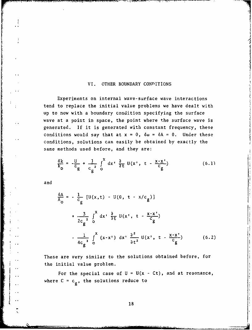
VI. OTHER BOUNDARY CONDITIONS

Experiments on internal wave-surface wave interactions

tend to replace the initial value problems we have dealt with

up to now with a boundary condition specifying the surface

wave at a point in space, the point where the surface wave is

generated. If it is generated with constant frequency, these

conditions would say that at x = 0, 6w = 6A = 0. Under these

conditions, solutions can easily be obtained by exactly the

same methods used before, and they are:

6k.. x x..x)+ - f dx' U(x' t .g (6.1)Cgc 2og

and

6A ~1AA _ cl [U(x,t) - U(0, t - x/cg)]

o gg

+ 3 fx dx' t U(x', t - I;

2c o gg

1 x a2 X-X'

1 (x-x') dx' 2-U(x', t (6.2)

4cg' 0 at 2 (.

These are very similar to the solutions obtained before, for

the initial value problem.For the special case of U = U(x - Ct), and at resonance,

where C = c the solutions reduce to

18

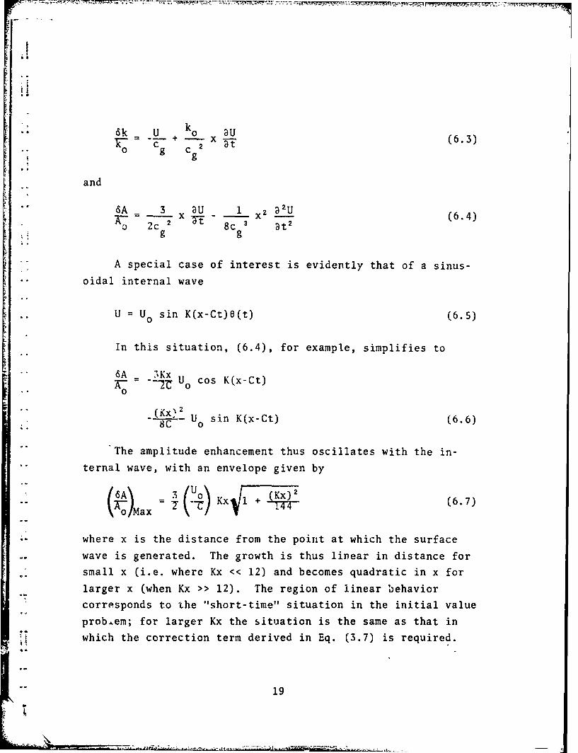
-; 6k =U- ko+ U6 g c 0 x 2 (6.3)

• g

and

SA _U3 1 x 2 (2U•." 6 •cax x- 8 t (6.4)

o c 8cg g

A special case of interest is evidently that of a sinus-

oidal internal wave

U = Uo sin K(x-Ct)O(t) (6.5)

In this situation, (6.4), for example, simplifies to

•"A = "--Kx U cos K(x-Ct)

;•: --- (Kx U0 .0

-- •ff_ U sin K(x-Ct) (6.6)8C 0

The amplitude enhancement thus oscillates with the in-

ternal wave, with an envelope given by

/•o/M•= rt"-e ¥ •(6.7)

where x is the distance from the point at which the surface

wave is generated. The growth is thus linear in distance for

small x (i.e. where Kx << 12) and becomes quadratic in x forlarger x (when Kx >> 12). The region of linear behaviorcorresponds to the "short-time" situation in the initial value

prob.em; for larger Kx the situation is the same as that inwhich the correction term derived in Eq. (3.7) is required.

"19

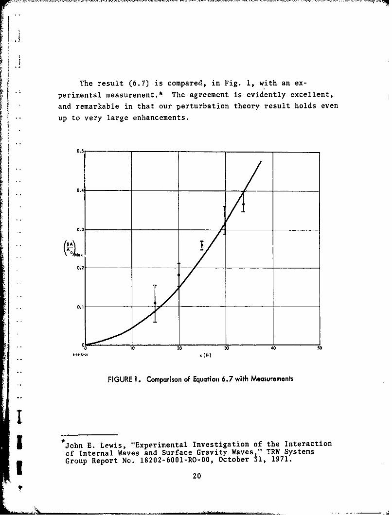
The resuit (6.7) is compared, in Fig. 1, with an ex-

perimental measurement.* The agreement is evidently excellent,

and remarkable in that our perturbation theory result holds even

up to very large enhancements.

0.5

0.3

0.2

T

0..,

"1030 o40 50

FIGURE 1. Comparison of Equation 6.7 with Measurements

--I *John E. Lewis, "Experimental Investigation of the Interactionof Internal Waves and Surface Gravity Waves," TRW Systems3 Group Report No. 18202-6001-RO-00, October 31, 1971.

20

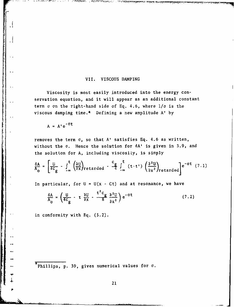
VII. VISCOUS DAMPING

Viscosity is most easily introduced into the energy con-

servation equation, and it will appear as an additional constant

term a on the right-hand side of Eq. 4.6, where 1/a is the

viscous damping time.* Defining a new amplitude A' by

A = A'e at

removes the term a, so that A' satisfies Eq. 4.6 as written,

without the a. Hence the solution for 6A' is given in 3.9, and

the solution for A, including viscosity, is simply

6A [U t(Uc t (7.1) a

0 g _0 Tx)retarded L0 (~~retarded]ea

In particular, for U = U(x - Ct) and at resonance, we have

6A U( t U t c 2U e'at-(72)T o 0 t 9- x 8X2 7 2

in conformity with Eq. (5.2).

Phillips, p. 39, gives numerical values for a.

•p