intermediate quality report - Национален …€¦ · web view · 2013-09-10this...

REPUBLIC OF BULGARIAREPUBLIC OF BULGARIANATIONAL STATISTICAL INSTITUTENATIONAL STATISTICAL INSTITUTE

INTERMEDIATE QUALITY REPORT

EU-SILC 2010 OPERATION

BULGARIA

SOFIA, December 2011

CONTENTS Pag

e

INTRODUCTION

1. COMMON CROSS-SECTION EUROPEAN UNION INDICATORS 31.1. Common cross-sectional EU indicators based on the cross-sectional component of EU-SILC

3

1.1.1. Primary Indicators calculated from SILC_2010 31.1.2. Secondary indicators of social cohesion calculated from SILC_2010 71.2. Other indicators 91.2.1. Equivalised disposable income 9

2. ACCURACY 102.1. Sample design 102.2. Sampling errors 142.3. Non-sampling errors 172.3.1. Sampling frame and coverage errors 172.3.2. Measurement and processing errors 172.3.3. Non-response errors 192.4. Mode of data collection 242.5. Interview duration 25

3. COMPARABILITY 253.1. Basic concepts and definitions 253.2. Components of income 273.2.1 Income definitions 273.2.2. The source or procedure used for the collection of income variables 303.2.3. The form in which income variables at component level have been obtained

30

3.2.4. The method used for obtaining income target variables in the required form

30

4. COHERENCE 314.1. Coherence of number of persons with external sources4.2. Comparison of some target variables from EU SILC 2009 survey with LFS20094.3. Comparison of EU-SILC 2009 and HBS 2009 results 4.4. Comparison of Laeken Indicators based on HBS 2008 and EU-SILC 2009 4.5. Comparison of some target variables from EU-SILC 2006, 2007, 2008 and 2009

3131323334

2

INTRODUCTION

The Survey on Income and Living Conditions (SILC) in Bulgaria is an annual survey implemented by the NSI in the framework of Regulation (EC) No 1177/2003 of the European Parliament and of the Council. Basic aim of the survey is the study, both at European and national level of households’ living conditions in relation to their income. The survey is the reference for comparative statistics on income distribution and social exclusion in the European Union.

In 2010, the survey was carried-out by the National Statistical Institute with the funds supplied by Eurostat grant nr. 10602.2009.003-2009.123.

This document presents the Intermediate Quality Report of EU-SILC 2010 in Bulgaria and follows the structure outlined in the Commission Regulation No. 28/2004.

The report is divided in four chapters:

(1) Common Cross-sectional European Union Indicators (2) Accuracy (3) Comparability (4) Coherence

1. COMMON CROSS-SECTIONAL EUROPEAN UNION INDICATORS

1.1. Common cross-sectional EU indicators based on the cross-sectional component of EU-SILC

The common cross sectional EU indicators refer to those indicators in Council of the Open method of coordination, based on the cross sectional sample of year 2010, with reference income period the calendar year (2009). The indicators below have been calculated using Eurostat SAS program.

1.1.1. Primary Indicators calculated from SILC_2010

Table 1. [OV-1a] At-risk-of poverty threshold (illustrative values)

Type of household Euro PPSOne person household 1810 3642Household with 2 adults end 2 children younger than 14 years 3801 7648

4

Table 2. [OV-1a] At-risk-of poverty rate after social transfers (by age and gender)

age sex unit 2010TOTAL T 1000PERS 1564.8 PC_POP 20.7 M 1000PERS 694.8 PC_POP 19.0 F 1000PERS 870 PC_POP 22.3Y0_17 T 1000PERS 340.6 PC_POP 26.8Y18_64 T 1000PERS 794 PC_POP 16 M 1000PERS 387.3 PC_POP 15.7 F 1000PERS 406.7 PC_POP 16.3Y65_MAX T 1000PERS 430.2

PC_POP 32.2 M 1000PERS 134.4 PC_POP 24.9 F 1000PERS 295.8 PC_POP 37.2

Table 3[PN-S1] At-risk-of-poverty rate of older people

age sex 2010Y_GE60 T 28.7 M 22 F 33.4Y_GE75 T 38.4 M 28 F 44.7Y_LT60 T 18.1 M 18.2 F 18Y_LT75 T 19.2 M 18.4 F 19.9

5

Table 4 [SI-S1a] At-risk-of-poverty rate, by household type

household type 2010TOTAL 20.7Households without dependent children 19.4One adult younger than 65 years 30.7One adult 65 years or older 61.6Single female 58.7Single male 34.5Two adults younger than 65 years 12Two adults, at least one aged 65 years and over 26.9Three or more adults 7.9Households with dependent children 21.7Single parent with dependent children 42.3Two adults with one dependent child 13.7Two adults with two dependent children 16.3Two adults with three or more dependent children 65.2Three or more adults with dependent children 21.9

Table 5 [SI-S1c] At-risk-of-poverty rate, by most frequent activity status and by gender

activity status sex age 2010Employment T Y_GE18 7.7 M Y_GE18 8.4 F Y_GE18 6.7Non employment T Y_GE18 32.4 M Y_GE18 30.6 F Y_GE18 33.6Unemployment T Y_GE18 48.3 M Y_GE18 51.9 F Y_GE18 44.7Retired T Y_GE18 30 M Y_GE18 23.6 F Y_GE18 34.2Inactive population - Other T Y_GE18 24.4 M Y_GE18 23.7 F Y_GE18 24.7

Table 6 [OV-2] Inequality of income distribution S80/S20 income quintile share ratio

6

age indic_il 2010

TOTAL S80_S20 5.9

Y_GE65 S80_S20 4.5

Y_LT65 S80_S20 5.9

Table 7. [OV-1b] Relative median at-risk-of-poverty gap (by age and gender)

age sex 2010TOTAL T 29.6 M 29 F 30.2Y18-64 T 29.6 M 29.9 F 29Y_GE65 T 26.6 M 20.7 F 29.2Y_GE75 T 29.5 M 23.2 F 31.7Y_LT18 T 36.5

Table 8 [OV-C11] At-risk-of-poverty rate before social transfers (by age and gender)

age sex 2010TOTAL T 40.8 M 38.6 F 42.8Y18-64 T 30.9 M 29.9 F 31.9Y_GE65 T 79.1 M 79.4 F 78.8Y_LT18 T 39

Table 9 [SI-C6] At-risk-of-poverty rate before social transfers, by gender and selected age groups (except pensions)

7

age sex 2010TOTAL T 27.1 M 25.4 F 28.8Y18-64 T 22.5 M 22.2 F 22.8Y_GE65 T 37.7 M 30 F 42.9Y_LT18 T 34.1

1.1.2. Secondary indicators of social cohesion calculated from EU-SILC

Table 10. [PEPS01] Population at risk of poverty or social exclusion by age and gender (ilc_peps01)

age sex unit 2010TOTAL T 1000PERS 3718.7 PC_POP 49.2 M 1000PERS 1729.3 PC_POP 47.3 F 1000PERS 1989.5 PC_POP 50.9Y18-64 T 1000PERS 2231.2 PC_POP 45 M 1000PERS 1085 PC_POP 44 F 1000PERS 1146.1 PC_POP 46Y_GE65 T 1000PERS 852.8 PC_POP 63.9 M 1000PERS 319.4 PC_POP 59.1 F 1000PERS 533.5 PC_POP 67.1Y_LT18 T 1000PERS 634.7 PC_POP 49.8

Table 11[PEES01] Intersections of Europe 2020 Poverty Target Indicators by age and gender

AGE sex indic_il unit 2010

8

TOTAL T NR_DEP_NLOW 1000PERS 2046.5 PC_POP 27.1 NR_NDEP_LOW 1000PERS 45.1 PC_POP 0.6 R_NDEP_NLOW 1000PERS 194.3 PC_POP 2.6Y18-64 T NR_DEP_NLOW 1000PERS 1343.7 PC_POP 27.1 NR_NDEP_LOW 1000PERS 38.3 PC_POP 0.8 R_NDEP_NLOW 1000PERS 88.1 PC_POP 1.8Y_LT18 T NR_DEP_NLOW 1000PERS 280 PC_POP 22 NR_NDEP_LOW 1000PERS 6.8 PC_POP 0.5 R_NDEP_NLOW 1000PERS 29.3 PC_POP 2.3

Table 12 People living in households with very low work intensity by age and gender

age sex unit 2010Y18-59 T 1000PERS 322.6 PC_POP 7.3 M 1000PERS 155.5 PC_POP 7 F 1000PERS 167.1 PC_POP 7.6Y_LT18 T 1000PERS 130.9 PC_POP 10.3Y_LT60 T 1000PERS 453.5 PC_POP 7.9 M 1000PERS 223 PC_POP 7.7 F 1000PERS 230.5 PC_POP 8.1

Table 13 [SI-P8]% of pop lacking at least 4 items in the economic strain and durables dimension by age and gender

age sex unit n_item 2010TOTAL T PC_POP GE4 45.7

9

M PC_POP GE4 44.2 F PC_POP GE4 47.2Y12-17 T PC_POP GE4 51.1 M PC_POP GE4 53.0 F PC_POP GE4 49.0Y18-64 T PC_POP GE4 42.2 M PC_POP GE4 41.5 F PC_POP GE4 42.9Y6-11 T PC_POP GE4 47.7 M PC_POP GE4 47.8 F PC_POP GE4 47.5Y_GE65 T PC_POP GE4 58.1 M PC_POP GE4 53.8 F PC_POP GE4 61.1Y_LT18 T PC_POP GE4 46.5Y_LT6 T PC_POP GE4 39.6 M PC_POP GE4 37.2 F PC_POP GE4 42.2

Table 14 [SI-S4] Mean number of items lacked by persons considered as deprived in the 'economic strain and durables' dimension by age and gender

age sex 2010TOTAL T 4.6 M 4.6 F 4.6Y18-64 T 4.5 M 4.6 F 4.5Y_GE65 T 4.6 M 4.4 F 4.6Y_LT18 T 4.8

1.2. Other indicators

1.2.1. Equivalised disposable income

National currency

Euro

Mean equivalised disposable income

6839.26 3496.91

Median equivalised disposable income

5898.41 3015.85

10

2. ACCURACY

2.1. Sample design

2.1.1. Type of sampling design

Four-year rotation panel is used for EU-SILC in Bulgaria. It contains 4 independent sub-samples and follows stratified two-stage cluster sampling design. Separated strata are formed based on the country administrative-territorial division. All private households in the country are covered.

2010 was the fifth year for the Bulgarian EU-SILC survey. In 2010 a new rotational group (number 8) with 2155 households was introduced.

2.1.2. Sampling units

Two stage sampling on a territorial principle is implemented as follows:- on the first stage - the census enumeration units (PSU) are selected; - on the second stage - the households are identified.

2.1.3. Stratification and sub-stratification criteria The general population and administrative-territorial division by statistical districts of the settlement, comprises all the households in the country. Population census 2001 data base was used as sampling frame. The sampling frame was updated according to the administrative changes occurred in human settlements statute in Bulgaria – some villages were recognized as towns; transition of municipalities or settlements from one administrative district to another.

The sample is stratified by administrative-territorial districts in the country (NUTS3) and the household’s location. As a result 56 strata are formed (28 of urban and 28 of rural population). Municipalities and settlements are ranged according to the number of their population within each stratum.

2.1.4. Sample size and allocation criteria

The necessary sample size for Bulgaria is determined in the Annex II of the Framework Regulation (1177/2003) to guarantee an effective sample size with regard to the at-risk-of-poverty indicator of 4500 households. The longitudinal sample for two successive waves should comprise at least 3500 households.

The total gross sample size (number of households) has been made analyzing the non-response rates and design effects of the previous EU-SILC surveys (2006-2009).

The total sample size in 2010 is 7354 households:-5064 “old” (longitudinal 2007, 2008 and 2009),

11

- 2155 “new” households (drawn in 2010).

2.1.5. Sample selection schemes

The number of census enumeration units (PSU) is calculated for each strata included in the sample.

The clusters on the first stage are chosen with probability proportion to population size (number of households) in the PSUs. Systematic sampling of secondary units (households) in each primary unitSelected is applied. Each PSU contains 5 households.

2.1.6. Sample distribution over time

As the survey is annual, the sample of households is not distributed over time. The survey is carried from May to July of the year 2010 with reference period of data the previous year (2009).

Table 15. Sample distribution (household questionnaire) over time

Month Data Number %May 11 –

20 57 0.921 –

31 579 9.4June 1 – 10 1071 17.4

11 – 20 858 13.9

21 – 31 1040 16.9

July 1 – 10 914 14.811 –

20 910 14.721 –

31 742 12.0Total 6171 100.00

2.1.7. Renewal of sample: rotational groups

Bulgaria applies a rotational panel in which the sample is divided into four sub-samples. Each of them is representing the whole population. Each year one of the rotation groups is dropped out and a new one is added to the sample.

2006 is the first year of EU-SILC in Bulgaria. The 6120 selected households are divided into 4 rotational groups with equal size. In 2007 the first rotational group R1(with a size 1530) is dropped out and 1530 new households are chosen.- R5. The rotational group R2 (with a size 1451) is dropped out in 2008 and 2935 new households are added as rotational group R6. In 2009 the third rotational group R3 (with a size 1072) is dropped out and 2915 new households are added as

12

rotational group R7. The rotational group R4 (with a size 894) is dropped out in 2010 and 2155 new households are added as rotational group R8.

Table 16. Size of rotational groups (selected sample)

Rotational group Year of survey

2006 2007 2008 2009 2010R1 1530 - - - -R2 1530 1451* - - -R3 1530 1444* 1072 - -R4 1530 1445* 1079 894 -R5 1530 1444* 974 941R6 2935 2571* 1863R7 2915 2260

R8 2155Total sample (households) 6120 5870 6530 7354 7219

*Including households which are not interviewed during the previous year

2.1.8. Weightings

Weighting factors were calculated as required to take into account the units’ probability of selection, non-response and to adjust the sample to external data relating to the distribution of households and persons in the target population, such as sex and age, residence or administrative-territorial districts (NUTS 3).

Design weights

For the first year of the panel, the design weights are equal to the inverses of the corresponding household inclusion probabilities. These weights are household design weights DB080.

For households in subsamples R5 (fourth year), R6 (third year) and R7 (second year) the household design factors were calculated by following general steps:

Computation of panel person base weights, coming from the final cross-sectional weight of the precedent year of survey;

Non-response adjustments due to panel attrition; Computation of base weights for persons entering panel households for the first time:

- children, born to sample women - the base weight is equal to the mother’s base weight;

- persons moving into sample household from outside the survey population – the base weight is the average of base weights of existing household members;

- persons moving into sample households from other non-sample households in the population have a basic panel weight equal to zero;

Computation of household weights by averaging within household over all household members.

13

Non-response adjustmentCorrection for non-response at the first year of subsamples R8 was done with Weighting within classes procedures:The design weights were modified by a factor inversely proportional to the response rate within strata. Coefficients of these corrections were computed separately according to classes of locality as ratios: the sum of design weights of selected units to the sum of design weights of responding units.

The response probability for the households at wave 2, 3, 4 ( subsamples R5, R6 and R7) is obtained by a logistic regression model. The following variables were used in the model:

• strata• size of household• sex• age group• activity• educational level• poverty indicators

Adjustments to external data (calibration)

After the non-response adjustments, the final weights were obtained applying the integrated calibration method. Combining the four independent subsamples, calibration is done on individual-level data, imposing equality of g-weights for individuals in the same household. We used truncated linear function in order to limit g-weights close enough to 1.

The following external information was used: Distribution of the population by administrative-territorial districts (NUTS 3) and

residence – urban/rural Distribution of the population by age groups (0 – 15, 16 – 19, 20 – 24, 25 – 29, 30 – 34,

35 – 39, 40 – 44, 45 – 49, 50 – 54, 55 – 59, 60 – 64, 65 – 69, 70 – 74, 75 or more), sex and residence – urban/rural

This information was derived from the Information System Demography (ISD).

Calibration was carried out with a G calib2.0 program (designed by Statistics Belgium).

Final cross-sectional weights

After calibration the final household cross-sectional weight DB090 is get.

The personal cross-sectional weight of an individual (RB050) is equal to the cross-sectional weight DB090 of its household.

Personal cross-sectional weights for all household members aged 16 and over (PB040) are obtained by correction for within household non-response of the RB050. After that the same calibration method as described above is used in order to adjust the weights to external sources.

14

2.1.9. Substitutions

No substitution was applied if the household did not enter the survey.

2.2. Sampling errors

2.2.1. Standard error and effective sample size

Computations of standard errors were carried out using JRR - SAS programs for variance estimation of the measures required for Intermediate quality Report

subpopulation est stat_se kish nHCR, after social transfers: Age 0-17 0.2677 0.0524 1.11 2034HCR, after social transfers: Age 18-24 0.1873 0.0125 1.13 1262HCR, after social transfers: Age 25-49 0.1583 0.0086 1.10 4752HCR, after social transfers: Age 50-64 0.1533 0.0070 1.15 3730HCR, after social transfers: Age 65+ 0.3231 0.0160 1.15 3716HCR, after social transfers: Male 0.1905 0.0073 1.14 7800HCR, after social transfers: Female 0.2234 0.0071 1.14 8517HCR, after social transfers: Male Age 0-17 0.2660 0.0157 1.11 1053HCR, after social transfers: Male Age 18-24 0.1891 0.0175 1.11 682HCR, after social transfers: Male Age 25-49 0.1573 0.0082 1.10 2405HCR, after social transfers: Male Age 50-64 0.1481 0.0081 1.15 1767HCR, after social transfers: Male Age 65+ 0.2492 0.0176 1.15 1492HCR, after social transfers: Female Age 0-17 0.2696 0.0151 1.11 981HCR, after social transfers: Female Age 18-24 0.1853 0.0134 1.15 580HCR, after social transfers: Female Age 25-49 0.1592 0.0102 1.10 2347HCR, after social transfers: Female Age 50-64 0.1579 0.0080 1.15 1963HCR, after social transfers: Female Age 65+ 0.3733 0.0182 1.15 2224HCR, after social transfers: Male Age 18+ 0.1755 0.0070 1.13 6747HCR, after social transfers: Female Age 18+ 0.2154 0.0072 1.13 7536HCR, after social transfers: Male Age 18-64 0.1588 0.0068 1.12 4854HCR, after social transfers: Female Age 18-64 0.1620 0.0070 1.13 4890HCR, after social transfers: Male Age 65+ 0.1803 0.0073 1.13 6308HCR, after social transfers: Female Age 65+ 0.1850 0.0070 1.14 6293HCR, after social transfers: One person hh under 65 years 0.3081 0.0201 1.22 489HCR, after social transfers: One person hh 65 years and over 0.6163 0.0272 1.15 999HCR, after social transfers: One person hh Male 0.3470 0.0210 1.20 458HCR, after social transfers: One person hh Female 0.5871 0.0267 1.21 1030HCR, after social transfers: One person hh Total 0.5095 0.0204 1.19 1488HCR, after social transfers: 2 adults no dependant children, both adults under 65 years 0.1195 0.0090 1.15 1682HCR, after social transfers: 2 adults no dependant children, at least one adult 65 years or more 0.2692 0.0244 1.16 2110

15

HCR, after social transfers: Other hh without dependant children 0.0786 0.0127 1.03 3094HCR, after social transfers: Single parent hh,one or more dependant children 0.4227 0.0329 1.17 318HCR, after social transfers: 2 adults one dependant child 0.1371 0.0248 1.15 1410HCR, after social transfers: 2 adults two dependant children 0.1628 0.0156 1.14 1416

HCR, after social transfers: 2 adults three or more dependant children 0.6516 0.0411 1.12 255HCR, after social transfers: Other hh with dependant children 0.2211 0.0127 1.09 4544HCR, after social transfers: Hh without dependant children 0.1940 0.0102 1.11 8374HCR, after social transfers: Hh with dependant children 0.2179 0.0093 1.12 7943HCR, after social transfers: Accommodation tenure status:Owner or rent free 0.2135 0.0070 1.14 15834HCR, after social transfers: Accommodation tenure status:Tenant 0.0598 0.0086 1.16 483HCR, after social transfers: Main activity status: Employed 0.0876 0.0049 1.14 6481HCR, after social transfers: Main activity status: Unemployed 0.4292 0.0255 1.16 1652HCR, after social transfers: Main activity status: Retired 0.2921 0.0127 1.15 5019HCR, after social transfers: Main activity status: Other inactive 0.2431 0.0105 1.12 3165HCR, after social transfers: Main activity status: Employed, Male 0.0949 0.0054 1.14 3466

HCR, after social transfers: Main activity status: Unemployed, Male 0.4313 0.0273 1.14 821

HCR, after social transfers: Main activity status: Retired, Male 0.2336 0.0146 1.16 2004

HCR, after social transfers: Main activity status: Other inactive, Male 0.2463 0.0127 1.13 1509

HCR, after social transfers: Main activity status: Employed, Female 0.0790 0.0054 1.13 3015

HCR, after social transfers: Main activity status: Unemployed, Female 0.4274 0.0279 1.17 831HCR, after social transfers: Main activity status: Retired, Female 0.3311 0.0141 1.15 3015

HCR, after social transfers: Main activity status: Other inactive, Female 0.2403 0.0124 1.11 1656HCR, after social transfers: Work intensity: hh without dependent children, w=0 0.8128 0.0220 1.09 502HCR, after social transfers: Work intensity: hh without dependent children, 0<w<1 0.2240 0.0111 1.13 5462HCR, after social transfers: Work intensity: hh without dependent children, w=1 0.0655 0.0158 1.15 1979HCR, after social transfers: Work intensity: hh with dependent children, w=0 0.4341 0.0211 1.16 3375HCR, after social transfers: Work intensity: hh with dependent children, 0<w<0.5 0.2517 0.0654 1.12 596HCR, after social transfers: Work intensity: hh with dependent children, 0.5<=w<1 0.0712 0.0059 1.10 2072HCR, after social transfers: Work intensity: hh with dependent children, w=1 0.0238 0.0023 1.02 2331HCR, before social transfers including pensions: Male Age 0-17 0.3443 0.0159 1.13 1053HCR, before social transfers including pensions: Male Age 18-24 0.2327 0.0155 1.13 682HCR, before social transfers including pensions: Male Age 25-49 0.2265 0.0093 1.12 2405HCR, before social transfers including pensions: Male Age 50-64 0.2140 0.0097 1.16 1767

16

HCR, before social transfers including pensions: Male Age 65+ 0.3013 0.0119 1.15 1492

HCR, before social transfers including pensions: Female Age 0-17 0.3520 0.0170 1.11 981




HCR, before social transfers including pensions: Female Age 65 + 0.4295 0.0116 1.15 2224HCR, before social transfers excluding pensions: Male Age 0-17 0.3913 0.0167 1.13 1053HCR, before social transfers excluding pensions: Male Age 18-24 0.2962 0.0178 1.12 682HCR, before social transfers excluding pensions: Male Age 25-49 0.2885 0.0101 1.11 2405HCR, before social transfers excluding pensions: Male Age 50-64 0.3121 0.0114 1.16 1767

HCR, before social transfers excluding pensions: Male Age 65+ 0.7951 0.0104 1.19 1492

HCR, before social transfers excluding pensions: Female Age 0-17 0.4035 0.0174 1.11 981




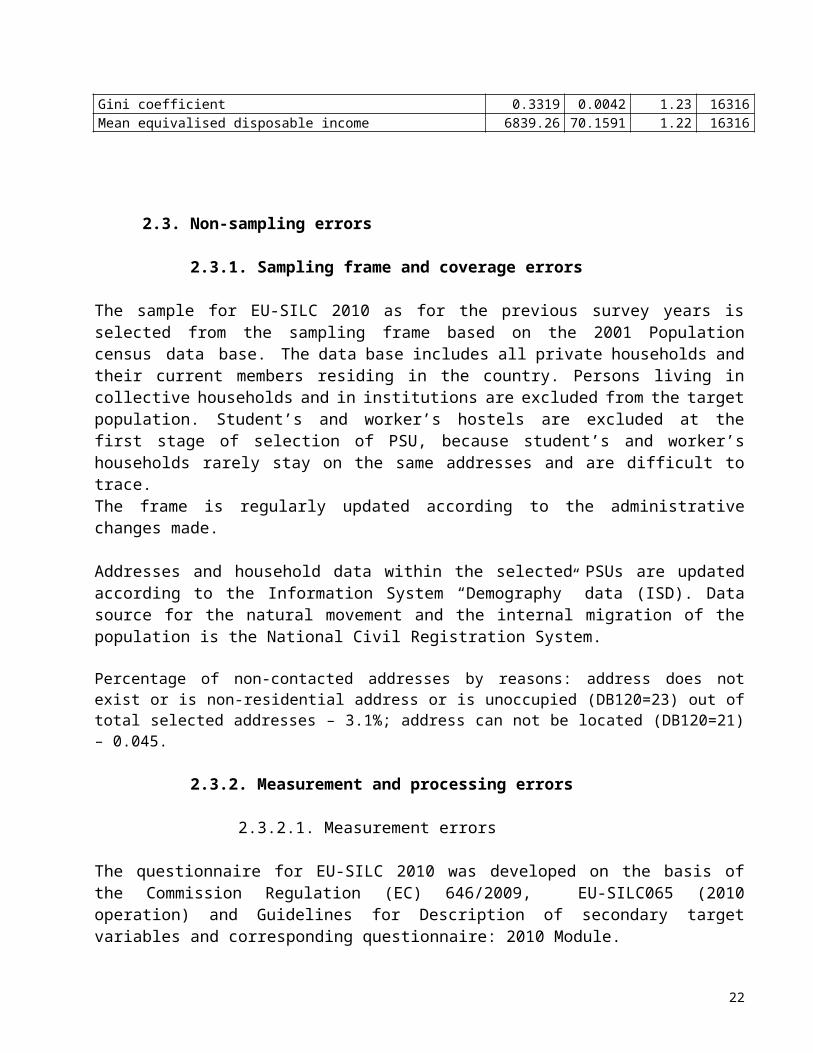
HCR, before social transfers excluding pensions: Female Age 65+ 0.7889 0.0092 1.17 2224Median equivalised disposable income 5898.41 95.0648 1.16 16317At-risk-of-poverty threshold, one person hh 2081.72 13.9384 1.19 1488At-risk-of-poverty threshold, hh 2 adults 2 dependent children 3670.99 87.6460 1.11 1416S80/S20 5.8464 0.2985 1.18 16317Relative median at-risk-of-poverty gap: Male Age 0-17 0.3765 0.0321 1.14 1053Relative median at-risk-of-poverty gap: Male Age 18-24 0.2956 0.0818 1.13 682Relative median at-risk-of-poverty gap: Male Age 25-49 0.3144 0.0219 1.13 2405Relative median at-risk-of-poverty gap: Male Age 50-64 0.2880 0.0190 1.18 1767Relative median at-risk-of-poverty gap: Male Age 65+ 0.2073 0.0442 1.15 1492Relative median at-risk-of-poverty gap: Female Age 0-17 0.3700 0.0336 1.11 981Relative median at-risk-of-poverty gap: Female Age 18-24 0.2674 0.0174 1.13 580Relative median at-risk-of-poverty gap: Female Age 25-49 0.3198 0.0241 1.15 2347Relative median at-risk-of-poverty gap: Female Age 50-64 0.2778 0.0208 1.19 1963Relative median at-risk-of-poverty gap: Female Age 65+ 0.2925 0.0107 1.15 2224Median income below the at-risk-of-poverty threshold 6839.26 42.4578 1.16 16316HCR P.L.as 50% median 0.1519 0.0065 1.14 16317HCR P.L.as 70% median 0.2826 0.0106 1.15 16317HCR P.L.as 40% median 0.0923 0.0041 1.16 16317Gini coefficient 0.3319 0.0042 1.23 16316Mean equivalised disposable income 6839.26 70.1591 1.22 16316

17

2.3. Non-sampling errors

2.3.1. Sampling frame and coverage errors

The sample for EU-SILC 2010 as for the previous survey years is selected from the sampling frame based on the 2001 Population census data base. The data base includes all private households and their current members residing in the country. Persons living in collective households and in institutions are excluded from the target population. Student’s and worker’s hostels are excluded at the first stage of selection of PSU, because student’s and worker’s households rarely stay on the same addresses and are difficult to trace. The frame is regularly updated according to the administrative changes made.

Addresses and household data within the selected PSUs are updated according to the Information System “Demography” data (ISD). Data source for the natural movement and the internal migration of the population is the National Civil Registration System.

Percentage of non-contacted addresses by reasons: address does not exist or is non-residential address or is unoccupied (DB120=23) out of total selected addresses – 3.1%; address can not be located (DB120=21) – 0.045.

2.3.2. Measurement and processing errors

2.3.2.1. Measurement errors

The questionnaire for EU-SILC 2010 was developed on the basis of the Commission Regulation (EC) 646/2009, EU-SILC065 (2010 operation) and Guidelines for Description of secondary target variables and corresponding questionnaire: 2010 Module.

EU-SILC survey in 2010 was carried out in May/July. EU-SILC is a non-obligatory, representative survey of individual households, performed by a face-to-face interview technique with the use of the PAPI method. Two types of questionnaires: individual and household questionnaire were applied. The fieldwork and all project implementation activities were done by NSI with annual grants from EC.

The training ship for interviewers was held on 15-18 March 2010. All responsible persons (supervisors) for the survey from each regional statistical office, interviewer and persons responsible for methodology from NSI took part in it. Household’s registries and person’s ID were marked with special attention. The training program included methodology, specific areas of income variables and variables from the new module 2010, which were presented to the participants. A discussion was held with the participants of the seminar related to the problems in collecting data and specific questions which required legislation knowledge. At the end of the course different examples of households and income sources were presented to the attendants and the training was evaluated.

18

Though some of the households have declared high income values, they confessed that their social insurance contribution is made at a lower amount. The data collected from the survey were compared to the data obtained from the registers. Some of the persons, who according to the register receive minimum income, defined themselves as unemployed or non-active in the survey, because they assess their current activity as temporary and did not indicate their income.

2.3.2.2. Processing errors

Data-entry phaseEU-SILC data were collected with two kinds of paper questionnaires – household and

individual questionnaire. The data entry program was developed in Visual Basic.Net. MS Access has been used as database.

A large number of edit checks (hard and soft) between questions in both questionnaires were implemented for ensuring data correctness and consistency. For example, two external files (at household and personal level) were used for verifying correctness of identifiers and for checking against previously collected information – household composition and questions such as day, month and year of birth, sex etc. for those individuals who are not observed for the first time. All gross income values were checked if they are equal or greater than net values (hard error) and if net values are greater or equal than gross values divided by two (soft error). In order to check the consistency of data on child allowances an additional check has been implemented – the program checks if the number and age of children in the household corresponds to the child allowances received in the household (hard error). Another check that has been added is between the salary of an individual, his/her profession and the minimum insurance income (soft error). According to national legislation the minimum insurance income is set to a certain level according to the profession type. For checking purposes, lower and upper boundaries, narrower than absolute, were set for most of the questions on income (e.g. social benefits, pensions) based upon national legislation. Internal files (implemented in the database) that hold valid ISCO-08 and NACE codes and descriptions were included.

During data entry phase, data entry operators were enabled to generate progress report by using SQL queries. The report contained form IDs, form status, number of errors and number of suppressed signals. A report for the number of individuals and households been interviewed or not grouped by interviewee had been added.

Data processing phaseAfter data-entry phase, further data checking and editing was performed by SILC unit, using

SPSS scripts.Initially, data were checked whether all questionnaires have been entered and completed.

Special attention was paid to split-off households. Next, all suppressed signals and remarks made by data entry operators were checked up and relevant corrections were made. After that, data were converted to SPSS data sets. Extreme income values were compared with data provided by National Social Security Institute or administrative data sources and data from previous waves, where possible and corrected if necessary. All SILC target variables were computed after checking original

19

variable(s). Finally, four transmission files were converted to .csv format and verified by Eurostat` SAS checking programs.

The main errors detected in the post-data-collection process were related to double registration of child allowances and personal income from agriculture, property or land. Both of them were recorded in household` and individual` questionnaires. As well as this, there were values that exceeded the maximum possible sizes of unemployment, old-age, survivor`, sickness and disability benefits.

All gross income values were checked if they are equal or greater than net values (hard error) and if net values are greater or equal than gross values divided by two (soft error).

The rates of failed edits for income variables are not available.2.3.3. Non-response errors

2.3.3.1. Achieved sample size

Table 17 Number of households for which an interview is accepted for the database. Rotational group breakdown and total

Rotational group

First wave Households

%

1 2007 882 14.32 2008 1765 28.63 2009 1975 32.04 2010 1549 25.1

Total 6171 100

Table 18 Number of persons of 16 years or older who are members of the households for which the interview is accepted for the database, and who completed a personal interview. Rotational group breakdown and total

Rotational group

First wave Households’ members

%

1 2007 2284 15.82 2008 4014 27.83 2009 4516 31.24 2010 3650 25.2

Total 14464 100.0

2.3.3.2. Unit non-response

New replication (4rd rotational group)

Household non-response rates NRh = [1 – (Ra*Rh)]*100, Ra = 0.995Rh = 0.756NRh = 24.8

Individual non-response rates NRp = (1 – Rp)*100,

20

Rp = 0.999NRp =0.14

Overall individual non-response rates *NRp = [1 – (Ra*Rh*Rp)]*100,*NRp = 24.9

Total sample

Household non-response rates NRh = [1 – (Ra*Rh)]*100,

Ra = Number of addresses successfully contacted = [DB120 = 11] 6928 . = 0.997

Number of valid addresses selected. [DB120 = all] - [DB120 = 23] 7177 - 69

Ra = 0.997Ra – the address contact rate

Rh = Number of household interviews completed and accepted for the database = [DB135=1] 6171 = 0.891 Number of eligible households at contacted addresses. [DB130=all] 6928

Rh = 0.891Rh – the proportion of complete household interviews accepted for the database

NRh=(1-0.997*0.891)*100= 11.21%

Individual non-response rates NRp = (1 – Rp)*100,

Rp = Number of personal interview completed = 14 464 = 0.998Number of eligible individuals 14 500

Rp – the proportion of complete personal interviews within the households accepted for the database

NRp=(1-0.998)*100=0.25%

Overall individual non-response rates *NRp = [1 – (Ra*Rh*Rp)]*100,

*NRp = [1- (0.997*0.891*0.998)]*100 = 11.43%;

- Information on non-response

total Rotation 1 Rotation 2 Rotation 3 Rotation 4All

householdsRa 0.997 1.000 0.999 0.995 0.995Rh 0.891 0.987 0.976 0.907 0.756

21

Rp 0.998 0.999 0.996 0.997 0.999NRp 0.25 0.13 0.40 0.27 0.14*NRp 11.43 1.34 2.43 9.93 24.91

Ra – the address contact rateRh – the proportion of complete household interviews accepted for the databaseRp – the proportion of complete personal interviews within the households accepted for the databaseNRp - Individual non-response rates*NRp - Overall individual non-response rates

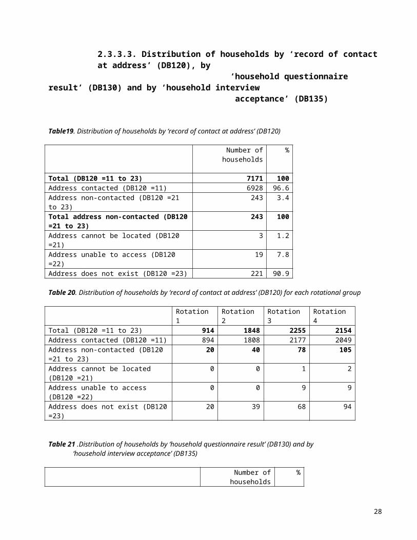
2.3.3.3. Distribution of households by ‘record of contact at address’ (DB120), by

‘household questionnaire result’ (DB130) and by ‘household interview acceptance’ (DB135)

Table19. Distribution of households by ‘record of contact at address’ (DB120)

Number of households

%

Total (DB120 =11 to 23) 7171 100Address contacted (DB120 =11) 6928 96.6Address non-contacted (DB120 =21 to 23)

243 3.4

Total address non-contacted (DB120 =21 to 23)

243 100

Address cannot be located (DB120 =21) 3 1.2Address unable to access (DB120 =22) 19 7.8Address does not exist (DB120 =23) 221 90.9

Table 20. Distribution of households by ‘record of contact at address’ (DB120) for each rotational group

Rotation 1 Rotation 2 Rotation 3 Rotation 4Total (DB120 =11 to 23) 914 1848 2255 2154Address contacted (DB120 =11) 894 1808 2177 2049Address non-contacted (DB120 =21 to 23)

20 40 78 105

Address cannot be located (DB120 =21)

0 0 1 2

Address unable to access (DB120 =22)

0 0 9 9

22

Address does not exist (DB120 =23)

20 39 68 94

Table 21 .Distribution of households by ‘household questionnaire result’ (DB130) and by ‘household interview acceptance’ (DB135)

Number of households

%

Total (DB130 =all) 6928 100Household questionnaire completed (DB130 =11)

6171 89.1

Interview not completed (DB130 =21 to 24)

757 10.9

Total interview not completed (DB130 =21 to 24)

757 100

Refusal to co-operate (DB130 =21) 317 41.9Entire household temporarily away (DB130 =22)

293 38.7

Household unable to respond (DB130 =23) 69 9.1Other reasons 78 10.3Household questionnaire completed (DB135=1+2)

6171 100

Interview accepted for database (DB135=1)

6171 100

Interview rejected (DB135=2 0 0

Table 22 .Distribution of households by ‘household questionnaire result’ (DB130) and by ‘household interview acceptance’ (DB135) for each rotational group

Rotation 1 Rotation 2 Rotation 3 Rotation 4Total (DB130 =all) 894 1808 2177 2049Household questionnaire completed (DB130 =11) 882 1765 1975 1549Interview not completed (DB130 =21 to 24) 12 43 202 500Refusal to co-operate (DB130 =21) 8 17 83 209Entire household temporarily away (DB130 =22) 3 14 97 179Household unable to respond (DB130 =23) 0 7 9 53Other reasons 1 5 13 59Household questionnaire completed (DB135=1+2) 882 1765 1975 1549

23

Interview accepted for database (DB135=1) 882 1765 1975 1549Interview rejected (DB135=2

2.3.3.4. Distribution of substituted units

No substitution was applied in our survey

2.3.3.5. Item non-response

Table 23 Information on item non-response on household level - households 2010

Item non-response

households having received an amount

Full information

Partial information

Missing information

total

% of all interviewed households total % total % total %

Total household gross income (HY010) 6169 100.0 1722 27.9 4368 70.8 85 1.4Total disposable household income (HY020) 6169 100.0 1719 27.9 4443 72.0 7 0.1Total disposable household income before social transfers except old-age and survivor’s benefits (HY022)

6143 99.5 2393 39.0 3733 60.8 17 0.3

Total disposable household income before social transfers including old-age and survivor’s benefit (HY023)

5879 95.3 3593 61.1 2264 38.5 22 0.4

Net income components at household level Income from rental of a property or land (HY040N) 934 15.1 930 99.6 4 0.4Family related allowances (HY050N) 1006 16.3 920 91.5 52 5.2 34 3.4Social exclusion not elsewhere classified (HY060N) 466 7.6 466 100.0Housing allowance (HY070) 1 0.0 1 100.0Regular inter-household cash transfer received (HY080) 707 11.5 707 100.0Alimonies received (HY081N) 64 1.0 64 100.0Interests, dividends, etc. (HY090N) 21 0.3 21 100.0Interest repayments on mortgage (HY100N) 259 4.2 259 100.0Income received by people aged < 16 (HY110) 45 0.7 45 100.0Taxes on wealth (HY120N) 4608 74.7 4608 100.0Regular inter-household cash transfer paid (HY130N) 861 14.0 852 99.0 4 0.5 5 0.6Tax on income and social contributions (HY140N) 3978 64.5 2936 73.8 474 11.9 568 14.3Value of goods produced by own-consumption (HY170N) 2114 34.3 2113 100 1 0.0Gross income components at household level Income from rental of a property or land (HY040G) 934 15.1 931 99.7 3 0.3Family related allowances (HY050G) 1006 16.3 920 91.5 52 5.2 34 3.4Social exclusion not elsewhere classified (HY060G) 466 7.6 466 100.0Housing allowance (HY070G) 1 0.0 1 100.0Regular inter-household cash transfer received (HY080G) 707 11.5 707 100.0Alimonies received (HY081N) 64 1.0 64 100.0Interests, dividends, etc. (HY090G) 21 0.3 21 100.0Interest repayments on mortgage (HY100G) 259 4.2 259 100.0Income received by people aged < 16 (HY110G) 45 0.7 45 100.0Taxes on wealth (HY120G) 4608 74.7 4608 100.0

24

Regular inter-household cash transfer paid (HY130G) 861 14.0 852 99.0 4 0.5 5 0.6Tax on income and social contributions (HY140G) 3978 64.5 2936 73.8 474 11.9 568 14.3Value of goods produced by own-consumption (HY170G) 2114 34.3 2113 100 1 0.0Net income component at personal levelEmployee cash or near cash income (PY010N) 7477 51.7 5047 67.5 1346 18.0 1084 14.5Net non-cash employee income (PY020N) 927 6.4 927 100.0Contribution to individual private pension plans (PY035N) 347 2.4 344 99.1 3 0.9Cash benefits or losses from self-employment (PY050N) 870 6.0 631 72.5 31 3.6 208 23.9Pension from individual private plans (PY080N) 40 0.3 40 100.0Unemployment benefits (PY090N) 653 4.5 233 35.7 420 64.3Old age benefits (PY100N) 4935 34.1 2346 47.5 2375 48.1 214 4.3Survivor’s benefits (PY110N) 109 0.8 109 100.0Sickness benefits (PY120N) 1465 10.1 48 3.3 14 1.0 1403 95.8Disability benefits (PY130N) 1333 9.2 469 35.2 340 25.5 524 39.3Education-related allowances (PY140N) 87 0.6 87 100.0 0.0Gross income components at personal level Employee cash or near cash income (PY010G) 7481 51.7 4603 61.5 1385 18.5 1493 20.0Net non-cash employee income (PY020G) 927 6.4 927 100.0Contribution to individual private pension plans (PY035G) 347 2.4 344 99.1 3 0.9Cash benefits or losses from self-employment (PY050G) 870 6.0 595 68.4 37 4.3 238 27.4Pension from individual private plans (PY080G) 40 0.3 40 100.0Unemployment benefits (PY090G) 653 4.5 233 35.7 420 64.3Old age benefits (PY100G) 4935 34.1 2346 47.5 2375 48.1 214 4.3Survivor’s benefits (PY110G) 109 0.8 109 100.0Sickness benefits (PY120G) 1465 10.1 48 3.3 14 1.0 1403 95.8Disability benefits (PY130G) 1333 9.2 469 35.2 340 25.5 524 39.3Education-related allowances (PY140G) 87 0.6 87 100.0 0.0Gross monthly earnings for employees (PY200G) 5625 38.9 5212 92.7 413 7.3

2.3.3.6. Total item non-response at unit level of the common cross-sectional European Union indicators based on the cross-sectional component of EU-SILC and for equivalised disposable income

Table 24. Item non-response at unit level of the common cross-sectional European Union indicators and for equivalised disposable income

Indicator Achieved sample size

Total item non-responce

At-risk-of-poverty rate after social transfers -total 16317 39

25

At-risk-of-poverty rate after social transfers -men total 7800 18At-risk-of-poverty rate after social transfers -women total

8517 21

At-risk-of-poverty rate after social transfers -0-17 years 2246 5At-risk-of-poverty rate after social transfers -18-64 years

10355 31

At-risk-of-poverty rate after social transfers -men 18-64 years

5145 17

At-risk-of-poverty rate after social transfers -women 18-64 years

5210 14

At-risk-of-poverty rate after social transfers -65+ years 3716 3At-risk-of-poverty rate after social transfers -men 65+ years

1492 1

At-risk-of-poverty rate after social transfers -women 65+ years

2224 2

At-risk-of-poverty threshold -single 1488 5At-risk-of-poverty threshold -2 adults, 2 children 1416 56

2.4. Mode of data collection

Table 25. Distribution of household members (RB245=1) by “Data status” (RB250)

Total Rotation 1 Rotation 2 Rotation 3 Rotation 4 N % N % N % N % N %Total 14500 100 2287 100 4030 100 4528 100 3655 100RB250=11 14461 99.7 2282 99.8 4013 99.6 4516 99.7 3650 99.9RB250=14 3 0.0 2 0.1 1 0.0 0 0 RB250=21 0 0 0 0 0 RB250=23 19 0.1 3 0.1 9 0.2 6 0.1 1 0.0RB250=31 12 0.1 0 4 0.1 5 0.1 3 0.1RB250=32 4 0.0 0 3 0.1 1 0.0 0 RB250=33 1 0.0 0 0 0 1 0.0

Table 26. Distribution of household members (RB245=1) by “Type of interview” (RB260)

Total Rotation 1 Rotation 2 Rotation 3 Rotation 4 N % N % N % N % N %

Total 14461 100.0 2282 100.0 4013 100.0 4516 100.0 3650 100.0Face to face (1)

11524 79.7 1797 78.7 3237 80.7 3554 78.7 2936 80.4

Proxy interview (5)

2937 20.3 485 21.3 776 19.3 962 21.3 714 19.6

The interviewers decided on proxy interviews only if the substitute respondents were well informed about the situation in the household and there was no other possibility to get the information. Proxy interviews were performed in the following situations:

26

- no contact with the respondent because of long-term absence (e.g. work in another town or abroad);

- respondent’s disability or illness; - the respondent was only available late at night and was not willing to

participate in such a long interview, while at the same time the proxy could provide detailed information, even based on the documents, such as tax statements.

2.5. Interview duration

The average household interview duration was about 28 minutes, while the average individual interview duration was about 22 minutes. The mean interview duration per household was estimated at 79.4 minutes.

3. COMPARABILITY

3.1. Basic concepts and definitions

There were no essential differences between the national concepts and standard EU-SILC concepts.

The reference population

The reference population is all citizens officially living at Bulgarian territory (population de facto). The source of the sample is the Census Population 2001. This Census includes all private households and their current members residing in the territory, independently of any socio-economic characteristics they may have. Persons living in collective households and in institutions are excluded from the target population.

The private household definition

The definition of household that Eurostat recommends is used. Household is defined as a person living alone or a group of people who live together in the same dwelling and share expenditures including the joint provision of the essentials of living. Family members living together but not sharing their income and expenditure with other family members make up separate households.

The household membership

All household members aged 16 years and more at the time of the interview, are selected for a personal interview.

The household composition accounted for:

27

1. Persons usually resident, related to other members 2. Persons usually resident, not related to other members 3. Resident boarders, lodgers, tenants 4. Visitors 5. Line-in domestic servants, au-pairs 6. Persons usually resident, but temporarily absent from the dwelling (for

reasons of holiday travel, work, education or similar) 7. Children of the household being educated away from home 8. Persons absent for long periods, but having household ties : persons working

away from home 9. Persons temporarily absent but having household ties: persons in hospital,

homes or other institutions

Further conditions for inclusion as household members are as follows:

(a) Categories 3,4, and 5: Such persons must currently have no private address elsewhere; or their actual or intended duration of stay must be six months or more.

(b) Category 6: Such persons must currently have no private address elsewhere and their actual or intended duration of absence from the household must be less than six months.

(c) Category 7 and 8: Irrespective of the actual or intended duration of absence, such persons must currently have no private address elsewhere, must be the partner or child of a household member and must continue to retain close ties with the household and must consider this address to be his/her main residence.

(d) Category 9: Such person must have clear financial ties to the household and must be actually or prospectively absent from the household for less than six months.

• Usually resident A person shall be considered as a usually resident member of the household if he/she spends most of his/her daily rest there, evaluated over the past six months. Persons forming new households or joining existing households shall normally be considered as members at their new location; similarly, those leaving to live elsewhere shall no longer be considered as members of the original household. The above mentioned ‘past six month’ criteria shall be replaced by the intention to stay for a period of six months or more at the new place of residence.

• Intention to stay for a period of six months or more

28

Account has to be taken of what may be considered as ‘permanent’ movements in or out of households. Thus a person who has moved into a household for an indefinite period or with their intention to stay for a period of six months or more shall be considered as a household member, even though the person has not yet stayed in the household for six months, and has in fact spent a majority of that time at some other place of residence. Similarly, a person who has moved out of the household to some other place of residence with the intention of staying away for six months or more, shall no longer be considered as a member of the previous household.

• Temporarily absent in private accommodation If the person who is temporarily absent is in private accommodation, then whether he/she is a member of this (or other) household depends on the length of the absence. Exceptionally, certain categories of persons with very close ties to the household may be included as members irrespective of the length of absence, provided they are not considered members of another private household.

In the application of these criteria, the intention is to minimize the risk that individuals who have two private addresses at which they might potentially be enumerated are not double-counted in the sampling frame. Similarly, the intention is to minimize the risk of some persons being excluded from membership of any household, even though in reality they belong to the private household sector.

The income reference period(s) used

The income reference period is a fixed twelve-month period, namely the previous calendar year. For SILC 2010 the income reference period is the year 2009

The period for taxes on income and social insurance contributions

The reference period for income tax repayment and compulsory social insurance contributions is the previous calendar year (2009).

The reference period for taxes on wealth

Taxes on wealth paid during the income reference period (2009) were recorded.

The lag between the income reference period and current variables

The income reference period is the previous calendar year (year 2009) and the current variables refer to the fieldwork period (May - July 2010). Therefore the lag is at minimum 5 months and at maximum 7 months.

29

The total duration of the data collection of the sample

EU-SILC was performed on the territory of the whole country between May and July 2010.

Basic information on activity status during the income reference period

There were no differences between the national concepts and standard EU-SILC concepts. This information can be obtained by combining the answer for question P2 (PL031) with the answer for question P25 (calendar question),(PL211A—PL211K)

3.2. Components of income

3.2.1 Income definitions

There are no differences between national definition and standard EU-SILC definition.

Within-household non-response inflation factor (HY025)In order to calculate variable HY025 the recommendation of the doc065 (EU-SILC 2010 Operation) were applied as follows:

HY025 = 1+ i/HY020cWhere HY020c is the collected household disposable income and i is a sum of imputed total personal income.

Imputed rent (HY030G)

Imputed rents are estimated for dwellings used as main residence by the households. The imputation is applied for those households that did not report paying rent:

- owners-occupiers- rent-free tenants

The market rent is the rent due for the right to use an unfurnished dwelling on the private market, excluding charges for heating, water, electricity, etc.

The stratification method used is based on actual rents (the same used by National Accounts – the same stratification variables and the same market rents). The method is in line with ESA’95 and requirements of Commission Decision 95/309 and Commission Regulation 1722/2005 on the principle of estimating dwelling services.

Stratification variables:- location (district centre with university, other district centre, smaller town, rural area) - size of the dwelling- number of rooms (1, 2, 3, 4+)

30

- amenities – availability of central heating

Actual market rents – main data sources:- current price statistics- household budget survey- real estate agencies

HY140G - Tax on income and social insurance contributionsThey are taxes on income and social insurance contributions paid for the previous calendar year 2009. The main problem of the survey EU-SILC is the provision of reliability of the data collected for the gross and net income of the interviewed persons. When the person does not respond to all questions connected with income it is necessary to convert net income into gross and vice versa. All incomes are different by source and form but their taxation and the payment of insurance contributions are subject to concrete rules.

According to the Social Insurance Code the insurance burden is divided between the employer and the insured person in a proportion defined by the Law for the Budget for the SSI for each calendar year. For 2009 this proportion is 60:40 (employer/insured, %). The insurance contributions for the respective funds are percentages from the insurance income as follows:

EMPLOYED PERSONS Employer Insured personFund “Pensions” (18%) 10.0 8.0Fund “General disease and maternity” (3.5%) 2.1 1.4Fund “Unemployment” (1%) 0.6 0.4Health insurance (8%) 4.8 3.2Fund “Work Injury and Occupational Disease” 0.7Fund “Earnings guarantee” 0.1

total 18.3 13.0SELF INSURED PERSONS person

Insured for pension Insured for all risks

Health insurance

XXX

18.0021.508.00

The insurance payments for the civil servants; the judges, prosecutors, investigators, state bailiffs, judges for the entries and court employees, as well as the members of the Supreme Judicial Council and the inspectors of the Inspectorate at the Supreme Judicial Council; the military servicemen under the Law of Defence and Armed Forces of the Republic of Bulgaria; the civil servants under the Law for the Ministry of Interior and the Law on Execution of Penalties and Detention and the civil servants referred to in the Law on State National Security Agency shall be for the account of the state budget, respectively the budget of the judicial authority

Insurance income includes all reimbursements and other incomes from labour activity. The law for the budget of SSI defines:

1. Minimal monthly insurance income during the calendar year. • minimal amount of the insurance income by economic activities and groups of professions according to which are to be insured the workers, employees, those working on contracts for

31

management and control of trade firms. The definition of the group of profession is done according to the National Classification of Professions. The working places are defined in 9 classes of professions and the post defines the type and contents of the labour activity of the person. • the minimal amount of the insurance income for self insured persons. For 2009 this monthly income is 260 BGN. They pay contributions on an amount of income chosen in advance in-between the minimum and maximum amount of income defined with the Law for the Budget of SSI.• The minimal amount of income for registered farmers and tobacco producers is 50% of the minimal insurance income (130 BGN) – the minimal amount of insurance income for registered farmers and tobacco producers who do only this activity is 25% of the minimal insurance income (65 BGN).

2. The maximal monthly amount of the insurance income for 2009 is 2000 BGN.

The main law, that defines income taxes, is the Law for Taxation of the Natural Persons’ Income (LTNPI). The fiscal year in the country is the calendar year. The tax unit is the person. Till April 30 2010 persons are obliged to fill in tax return forms or as they are called in Bulgaria - tax declarations (TD) and 30 days later should pay the balance of the income tax due or in case they have paid more tax in advance – get paid back for the negative balance.

The tax on the annual tax base is being assessed by multiplying the annual tax base by the 10% tax rate. The income from economic activity as a sole proprietor shall be taxed separately, with a tax on the annual tax base at the tax rate of 15%.

Incomes for which no income tax is due Income from a small family business for which a fixed (patent) tax is paid at the beginning of

the fiscal year. Income from interest on savings. Income from pensions. Income from social benefits – family, unemployment and other benefits. Incomes from fellowships and scholarships.

3.2.2. The source or procedure used for the collection of income variables

Total gross income and disposable household income were calculated according to Document 065 (2010 operation). All personal/household income variables were collected by interview.

In some cases, where the information on income component is unavailable a register to obtain missing value information is used. The National Social Security Institute keeps a register of all persons for whom employers pay social insurance contributions and of all self-insured persons. This register contains some data on personal income but it is generated by a labour activity of the persons and moreover, this is only the income on which the person was insured.

3.2.3. The form in which income variables at component

32

level have been obtained

The interviewers and the respondents have the option of reporting income gross and/or net at component level. The form in which the net amounts are recorded in database are net of tax on income at source and of social contributions.

3.2.4. The method used for obtaining income target variables

in the required form

The gross income was obtained by summing up net value, income tax payments and compulsory social insurance contributions. If the information on tax and insurance contributions was missing, the amounts were imputed in accordance with the labour and social insurance legislations.

If either the net or the gross value was missing for PY010, PY050 or PY100, the missing value was calculated on the basis of a net-gross conversion and vice versa.

4. COHERENCE

4.1. Coherence of number of persons with external sources

Table 27. Coherence of number of persons with external sources

SILC 2010Other source Source

Population 7 563 710 7 563 710 Population as of 31.12.2010 male 3 659 311 3 659 311 female 3 904 399 3 904 399

Mean number of pensioners 1 717 653 2 192 524 NSSIHouseholds sharing of expenditures 2 614 503 3 080 549 LFS 2010Employed 3 276.8 3 052.8 LFS 2010Working full time 3 143.1 2 980.9 LFS 2010Working part-time 133.7 72.0 LFS 2010Unemployed 679.7 348.0 LFS 2010Economically inactive 2 508.2 3 136.7 LFS 2010

4.2. Comparison of some target variables from EU SILC 2010 survey with LFS2010

33

Table 28. Highest ISCED level attainedPE040 Highest ISCED level attained SILC 2010 LFS 2010Weighted PB040 % total % total1 – primary education 6.9 443.1 6.6 434.42 – lower secondary education 23.8 1 538.1 26.4 1 728.43 – upper secondary education 49.1 3 177.2 48.3 3 157.64 - post-secondary non tertiary education 0.6 39.8 0.5 31.05 – first stage of tertiary education 18.2 1 174.2 18.0 1 174.66 – second stage of tertiary education 0.3 18.5 0.2 11.6missing value 1.1 73.8

Table 29. Self-defined current economic statusPL030 Self-defined current economic status SILC 2010 LFS 2010Weighted PB040 % total % totalemployed (PL031 = 1,2,3,4) 50.7 3 276.8 46.4 3 032.9unemployed (PL031=5) 10.5 679.7 9.6 627.5economically inactive (PL031=6,7,8,9,11) 38.8 2 508.2 44.0 2 877.1

Table 30. Status in employmentPL040 Status in employment (PL031=1,2,3,4) SILC 2010 LFS 2010Weighted PB040 % total % total Employed (PL031 = 1,2,3,4) 100 3 276.3 100 3 052.8 employees 87.6 2 871.1 87.5 2 662.8 self-employed without employees 7.9 258.0 8.0 242.7self-employed with employees 4.0 129.9 3.5 115.1 family worker 0.5 17.3 1.0 32.2missing value 0.5

4.3. Comparison of EU-SILC 2010 and HBS 2010 results

The objective of this section is to compare HBS (Household Budget Survey) and EU-SILC results. When comparing these two sources we must take into account the discrepancies. The differences are to great extent brought about by the methodological diversity. Here are the main methodological differences:

- Different reference periods for income variables – in HBS the main variables of income is estimated quarterly and yearly and presented in the form of average values. In EU-SILC the reference period is the previous calendar year;

- Different types of income are taken into account i.e. in HBS the information is collected both about the income in cash and in kind, while in EU-SILC – only about the income in cash (with a few exceptions), which may be important for the income from farming and social benefits other than retirement pay and pension;

- Different way of data collection – in HBS the respondents make records in the so called diary. They have to determine the data sources themselves and do not have them listed in the diary. In EU-SILC each respondent is asked

34

detailed questions. In EU-SILC all the income missing data are imputed, while there is no imputation in HBS;

- HBS data are not weighted.

Table 31. Household by size,%Households type HBS 2010 EU-SILC 2010One person household 24.8 24.2Two persons household 34.1 32.2Three persons household 20.1 18.1Four or more person household 21.0 25.5

Table 32. Structure of population by age % Structure of population by age, % HBS 2010 EU-SILC 20100-15 10.9 11.316-24 9.3 11.125-49 28.0 30.550-64 23.1 24.365+ 28.7 22.7

Table 33. Structure of population by level of education, % Structure of population by level of education, % HBS 2010 EU-SILC 2010Primary education 15.1 12.5Lower secondary 22.6 26.6Upper secondary 46.5 44.0Tertiary education 15.8 16.9

Table 34. Activity status,%Activity status, % HBS 2010 EU-SILC 2010Employed 35.7 40.0Unemployed 11.9 9.1Economically inactive 52.4 50.9

Table 35. Status in employment, %Status in employment, % HBS 2010 EU-SILC 2010Employer 1.6 2.6Self-employed 6.0 5.4Employee 92.1 91.7Family worker 0.3 0.3

Table 36. Dwelling typeDwelling type HBS 2010 EU-SILC 2010Detached house 44.6 47.4Semidetached house 8.7 10.5Apartment or flat 46.4 41.6Some other kind of accommodation 0.3 0.5

Table 37. Non monetary household deprivationNon monetary household deprivation“Cannot afford”

HBS 2010 EU-SILC 2010

Telephone 0.9 3.9Color TV 0.8 3.0

35

Computer 14.3 21.8Washing machine 14.0 15.9Car 22.5 25.3

4.4. Comparison of Laeken Indicators based on HBS 2009 and EU-SILC 2010

Table 38. Main indicators – comparability – HBS and EU-SILC

Main indicators HBS 2009 EU-SILC 2010At-risk-of poverty threshold - Euro 1415.00 1810Household with 2 adults end 2 children younger than 14 years 2971.4 3801At-risk-of poverty rate after social transfers. % 14.7 20.7Relative median at-risk-of poverty gap after social transfers 21.3 29.6S80/S20 quintile share ratio 3.9 5.9At-risk-of-poverty rate before social transfers. % 46.9 40.8Dispersion around et-risk-of-poverty threshold 40% of median 5.0 9.250% of median 8.5 15.270% of median 22.6 28.3Gini coefficient 26.2 33.2At-risk-of-poverty rate before social transfers (except pensions).% 18.4 27.2

[SI-S1a] At-risk-of-poverty rate, by household typeTotal 14.7 20.7Households without dependent children 12.8 19.4One adult younger than 64 years 33.2 30.7One adult older than 65 years 34.6 61.6Single female 35.7 58.7Single male 27.6 34.5Two adults younger than 65 years 8.9 12.0Two adults, at least one aged 65 years and over 5.7 26.9Three or more adults 9.7 7.9Households with dependent children 16.9 21.7Single parent with dependent children 27.5 42.3Two adults with one dependent child 9.3 13.7Two adults with two dependent children 15.7 16.3Two adults with three or more dependent children 42.4 65.2Three or more adults with dependent children 20.0 21.9

4.5. Comparison of some target variables from EU-SILC 2007, 2008, 2009 and 2010

Table 39. Self-defined current economic status

PL030 (weighted PB040) EU SILC 07 EU SILC 08 EU SILC 09 EU SILC 10 % total % total % total % total employed (PL030 = 1,2) 46.8 3 069 463 51.3 3 350 418 52.0 3 381 702 50.7 3 276 791

36

unemployed (PL030 = 3) 14.8 968 576 9.5 617 814 9.6 623 495 10.5 679 719economically inactive (PL030=4,5,6,7,8,9) 38.3 2 511 575 39.2 2 564 718 38.4 2 501 406 38.8 2 508 162 missing 0.1 9 741 0 1 454

Table 40. Status in employment

PL040 (weighted PB040) EU SILC 07 EU SILC 08 EU SILC 09 EU SILC 10(PL030=1,2) % total % total % total % total Employed (PL030 =1,2) 100 3 069 463 100 3 350 418 100 3 381 702 100 3 276 291 employees 91.0 2 793 907 86.6 2 902 147 86.9 2 939 546 87.6 2 871 057 self-employed without employees 1.4 43 343 4.5 151 051 4.0 136 202 7.9 257 982self-employed with employees 5.4 166 765 7.8 260 189 8.3 281 064 4.0 129 940 family worker 0.7 20 522 1.1 35 867 0.7 24 890 0.5 17 312 missing 1.5 44 926 0 1 164 500

Table 41 Personal income

weight pb040

EU SILC 08 EU SILC 09 EU SILC 10

totalMean

totalMean

totalMean

N G N G N GPY010 3 527 483 4047.09 5389.49 3 303 963 5442.37 7204.56 3 639 408 5365.50 6602.82PY020G/N 496 833 502.52 523 611 582.02 467 115 868.91 PY050 486 646 6992.48 7771.75 409 832 8411.39 9539.95 401 585 7098.5 8749.74PY100G/N 1 762 552 2141.72 1 714 686 2751.88 1 793 001 3211.77

37

intermediate quality report - Национален …€¦ · web view · 2013-09-10this...

Documents