intermediate macroeconomics - winter 2014
TRANSCRIPT

INTERMEDIATEMACROECONOMICSMACROECONOMICS
- WINTER 2014 -Francesco Trebbi
1 Macroeconomics 302 - Lecture 1

Welcome to the Study of the Aggregate Economy
This is Macroeconomics and here are some interesting objectives/questions:
1 Understanding (and forecasting) short run fluctuations (the Business Cycle)1. Understanding (and forecasting) short-run fluctuations (the Business Cycle)
2. Studying the long-run performance of the economy (Economic Growth)
3. What determines Unemployment?
4. What drives price changes (Inflation)?
5. What is the role for economic policy and the government? (Monetary and Fiscal Policy)
6. How does the domestic economy interact and how is it influenced by the rest of the world?
N W ’ll i d i h l f h US ( l i l ) d C d
Macroeconomics 302 - Lecture 12
Note: We’ll motivate our study with examples from the US (mostly in class) and Canada (mostly in the textbook).

US Business Cycle and Economic Growth Real GDP 1/1948 – present
Black line - trend in real GDP over time (black axis) – defined later in the lectureRed line - trend in real GDP growth (percentage change in real GDP) over time
Macroeconomics 302 - Lecture 13
(right axis)Shaded areas represent “official” recession dates (as calculated by National Bureauof Economic Research)

US Historical Unemployment: 1/1970 – present
Macroeconomics 302 - Lecture 14
Shaded Areas – Recession Years

US Historical Inflation: 1/1948 – present (Annualized)
Macroeconomics 302 - Lecture 15
Shaded Areas – Recession Years
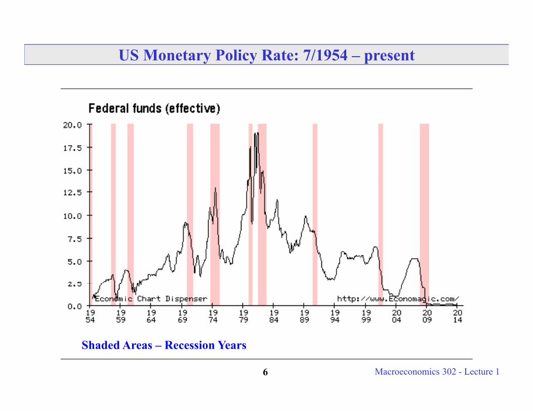
US Monetary Policy Rate: 7/1954 – present
Macroeconomics 302 - Lecture 16
Shaded Areas – Recession Years

US Monetary Policy Rate: 7/1954 – present
Macroeconomics 302 - Lecture 177
Shaded Areas – Recession Years

Recent US Monetary Action under Ben Bernanke
Macroeconomics 302 - Lecture 18
Shaded Areas – Recession Years

Understanding what the Federal Reserve says
Federal Reserve: FOMC Press Release Release Date: March 18, 2008 For immediate release The Federal Open Market Committee decided today to lower its target for the federal funds rate
75 basis points to 2-1/4 percent.Recent information indicates that the outlook for economic activity has weakened further. GrowthRecent information indicates that the outlook for economic activity has weakened further. Growth
in consumer spending has slowed and labor markets have softened. Financial markets remain under considerable stress, and the tightening of credit conditions and the deepening of the housing contraction are likely to weigh on economic growth over the next few quarters.
Inflation has been elevated, and some indicators of inflation expectations have risen. TheInflation has been elevated, and some indicators of inflation expectations have risen. The Committee expects inflation to moderate in coming quarters, reflecting a projected leveling-out of energy and other commodity prices and an easing of pressures on resource utilization. Still, uncertainty about the inflation outlook has increased. It will be necessary to continue to monitor inflation developments carefully.f p f y
Today’s policy action, combined with those taken earlier, including measures to foster market liquidity, should help to promote moderate growth over time and to mitigate the risks to economic activity. However, downside risks to growth remain. The Committee will act in a timely manner as needed to promote sustainable economic growth and price stability.
Macroeconomics 302 - Lecture 19
y p g p y We will understand what they mean
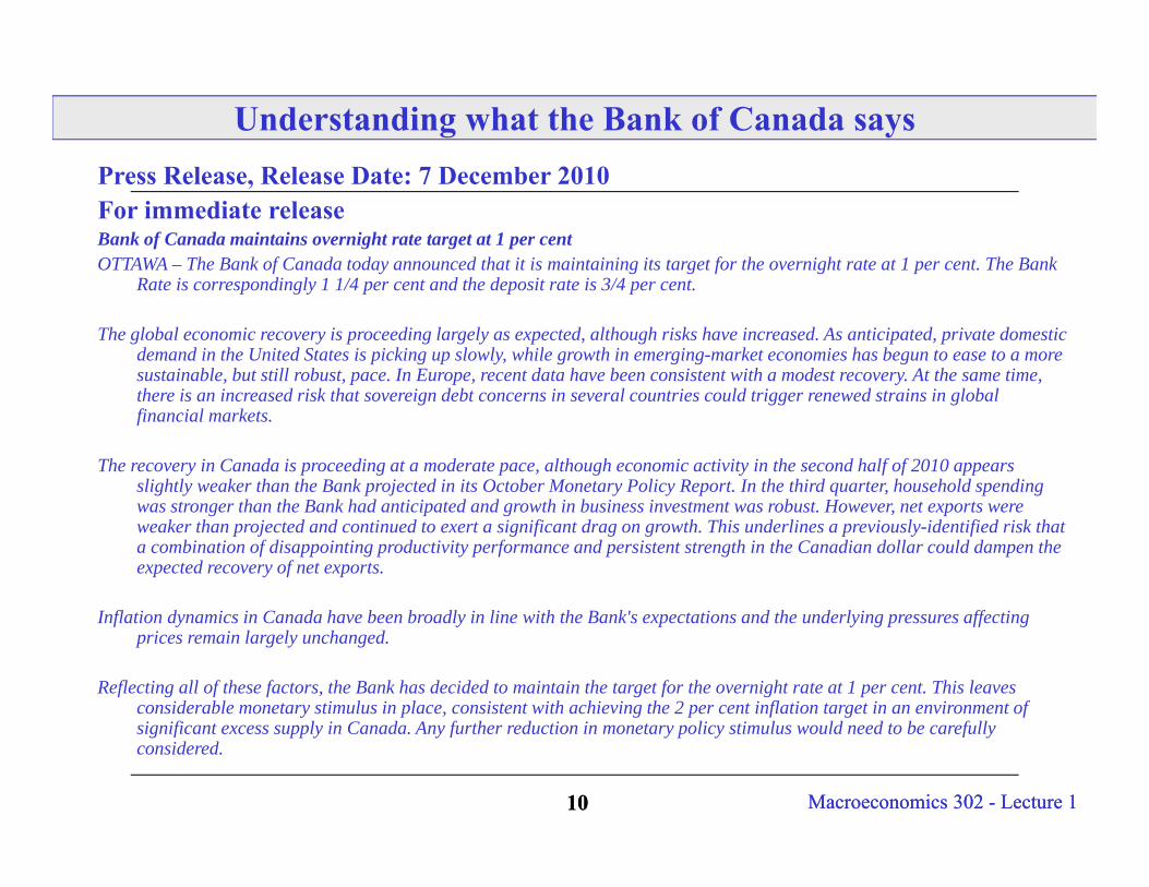
Understanding what the Bank of Canada saysPress Release, Release Date: 7 December 2010For immediate release Bank of Canada maintains overnight rate target at 1 per cent OTTAWA – The Bank of Canada today announced that it is maintaining its target for the overnight rate at 1 per cent. The Bank
Rate is correspondingly 1 1/4 per cent and the deposit rate is 3/4 per cent.
The global economic recovery is proceeding largely as expected, although risks have increased. As anticipated, private domestic demand in the United States is picking up slowly, while growth in emerging-market economies has begun to ease to a more sustainable, but still robust, pace. In Europe, recent data have been consistent with a modest recovery. At the same time, there is an increased risk that sovereign debt concerns in several countries could trigger renewed strains in global financial markets.
The recovery in Canada is proceeding at a moderate pace, although economic activity in the second half of 2010 appears slightly weaker than the Bank projected in its October Monetary Policy Report. In the third quarter, household spending
h h B k h d d d h b b Hwas stronger than the Bank had anticipated and growth in business investment was robust. However, net exports were weaker than projected and continued to exert a significant drag on growth. This underlines a previously-identified risk that a combination of disappointing productivity performance and persistent strength in the Canadian dollar could dampen the expected recovery of net exports.
I fl i d i i C d h b b dl i li i h h B k' i d h d l i ff iInflation dynamics in Canada have been broadly in line with the Bank's expectations and the underlying pressures affecting prices remain largely unchanged.
Reflecting all of these factors, the Bank has decided to maintain the target for the overnight rate at 1 per cent. This leaves considerable monetary stimulus in place, consistent with achieving the 2 per cent inflation target in an environment of i ifi t l i C d A f th d ti i t li ti l ld d t b f ll
Macroeconomics 302 - Lecture 110 Macroeconomics 302 - Lecture 110
significant excess supply in Canada. Any further reduction in monetary policy stimulus would need to be carefully considered.

Federal Budget Deficit
Macroeconomics 302 - Lecture 111

Thoughts on Economic Outlook (2011 est.)
In 2011 the US economy (production) was about $15.8 trillion (CAN $1.39 trillion) Population 313 million, labor force 155 million. (CAN 34 million) US Output per capita $48,300 (CAN $40,500) Inflation rate 3.1% (CAN 2.9%) Unemployment rate 9% (CAN 7.5%)
$2 3 illi G di $3 6 illi Tax revenues $2.3 trillion; Gov Expenditures $3.6 trillion. Gov. Deficit 8.7% of GDP (CAN 4.7%); Gov. Debt 67.8% of GDP (CAN 87.4% ) Spending of Economic Agents (Consumers and firms spend when they are
optimistic about the future).optimistic about the future).
• Consumers (~ 70% of the U.S. economy) (~ 55% of the CAN economy)• Business (~ 16% of the U.S. economy) (~ 20% of the CAN economy)
• Government (~ 17% of the U.S. economy) (~ 22% of the CAN economy)• Foreign Sector (~ -3% of the U.S. economy) (~ +3% of the CAN economy)
Macroeconomics 302 - Lecture 112

Real Household Spending: 1/1999 – present (Consumption)
Black Line Le el of Spending (Left A is)
Macroeconomics 302 - Lecture 113
Black Line – Level of Spending (Left Axis)Red Line – Percentage Change in Spending over Prior 12 months (Right Axis)Shaded Areas – Recession Years

Real Business Spending: 1/1999 – present (Investment)
Black Line Le el of Spending (Left A is)
Macroeconomics 302 - Lecture 114
Black Line – Level of Spending (Left Axis)Red Line – Percentage Change in Spending over Prior 12 months (Right Axis)Shaded Areas – Recession Years

US Balance on Current Account: 1960Q1 – present
Black Line – Current Account Balance Shaded Areas Recession Years
Macroeconomics 302 - Lecture 115
Shaded Areas – Recession Years

Thoughts on the Current Economic Outlook
Are we still in a de facto recession? Unemployment rate? (overall health of the U.S./CAN economy?)
Spending of Economic Agents
• Consumers• Business• Government• Foreign Sector
Other Things on My Mind:
EU C i i• EU Crisis• 2014 Unemployment rates• Housing Market still down-weighting on growth.• Central Bank Oversight and political influence on Monetary Policy
Macroeconomics 302 - Lecture 116
• Central Bank Oversight and political influence on Monetary Policy

Deflation Risks in EU?
Macroeconomics 302 - Lecture 117Source: Wall Street Journal

EU Crisis
Macroeconomics 302 - Lecture 118Source: Economist

Housing Prices
Macroeconomics 302 - Lecture 119Source: WSJ

Interesting Questions We Will Address This Term
What determines a country’s output? What determines consumption choices?
How do countries grow over long periods of time? Why do some countries grow faster than others? Why has Japan stagnated during the last two decades?
Can rising oil prices increase the inflation rate? If so, how? Why do we care about rising inflation rates? What can the Federal Reserve do to mitigate rising inflation rates? Is there a cost to their policy? What happens in oil exporting
i ?countries?
What is the role of the Central Bank in the macroeconomy? How do they i fl i t t t ? H d i t t t ff t l tinfluence interest rates? How do interest rates affect unemployment, production, etc.? How’s Bernanke’s regime different from Greenspan’s? Should the Fed follow explicit policy rules (i.e., target a 2% inflation rate –always) or should they follow some discretion?
Macroeconomics 302 - Lecture 120
y ) y

Interesting Questions We Will Address This Term
What are the role of labor markets in the economy? What is a “job-less” recovery? Is this a new phenomenon? (Yes)
Has the U.S. economy become more stable during the last 25 years? (Yes/No). Why? Has macro policy gotten better? (Yes/No) Have fundamentals in the economy changed? (Yes)(Yes)
Does the executive have significant impact on the economy in the short run? (Not really) Can they affect the economy in the long run? (Yes) Can large budget deficits hi d i th i th l ? (Y ) Wh ?hinder economic growth in the long run? (Yes) Why?
Should macro economists care about current account deficits? (Sometimes) Why could large trade deficits be a good thing for an economy? How important is outsourcing?large trade deficits be a good thing for an economy? How important is outsourcing?
Other topics: What role do consumers play in the macroeconomy? Can a housing slump cause a (severe) recession? How would social security reform affect the macroeconomy? L i t ?
Macroeconomics 302 - Lecture 121
Low savings rates?

Course Preliminaries
Quizzes: I’ll post online quiz material. Not graded, but useful for exercise and self-evaluation. Use it as preparation material or for furthering your understanding. No graded homework. If you need that kind of i iti t k thi i t limposition to keep up, this is not your class.
Midterms: 1st Midterm on February 11th – Will last 1h 20’!2nd Midterm on March 11th – Will last 1h 20’!
Final: UBC sets the date. No alternative arrangements.
Grading Policy: 100% midterms and final.I count each midterm ‘once’I count each midterm once .I count final ‘three times’.In total, I will have five observations for midterms and finals. I will keep the three highest observations and average them.
This implies that the midterms are optional (although, I strongly encourage you to take them – much easier than the final).If you wish to get provisional grades you need to take the midterms.
Macroeconomics 302 - Lecture 122
Readings/Must Reads: Assigned (encouraged). I will try to link to lectures. “Readings are Fair Game For All Tests”

Course Preliminaries (continued)
In Class: I really appreciate your participation. This is a hard class, so be prepared to answer direct questions –this way I can check if you’reprepared to answer direct questions this way I can check if you re getting it. If you do not like cold-calling, this is not your class.
Teaching Assistant: Crystal Li [email protected] first resource for simple questions on the materialYour first resource for simple questions on the material.
Lecture Notes: I upload them online before class. They are comprehensive anddetailed. All material is posted on my webpage:
http://faculty.arts.ubc.ca/ftrebbi/302_trebbi.html
Macroeconomics 302 - Lecture 123
An Introduction to Macro Data:The National Economy
Topic 1
Macroeconomics 302 - Lecture 124

Topic 1: Outline and Goals
(1) How do we Measure Current Economic Activity? (Simon Kuznets, Nobel 1971) What is Gross Domestic Product (GDP)? Why do we care about it? How do we measure standards of living over time? What are the definitions of the major economic expenditure components?
(2)(2) What is the difference between ‘Real’ and ‘Nominal’ variables? How is Inflation measured? Why do we care about Inflation?
(3)(3) What have been the predominant relationships between Unemployment, Inflation and GDP over the last four decades.
(4)(4) Nominal and Real Interest Rates. The Yield Curve. How is Unemployment measured? Why do we care about Unemployment?NOTE Thi l t ill lik l i t t k Thi i b d i It d t
Macroeconomics 302 - Lecture 125
NOTE: This lecture will likely go into next week. This is by design. It does not mean we will be short-changed on other material later in the class.

Objective: Measuring the amount of Economic ActivityActivity
3 Approaches of Measuring the amount of Economic Activity:
1) Product approach:Add the MKT Value of Goods & Services Produced Minus the Value of
Intermediate Materials across all industries (VALUE ADDED)Intermediate Materials across all industries. (VALUE ADDED)
2) Income approach: Add the Income Received by All Producers of Output (wages forAdd the Income Received by All Producers of Output. (wages for
workers and profits for owners of firms)
3) Expenditure approach:3) Expenditure approach:Add the Amount Spent by All Ultimate Users of Output. (Final Consumers)
They are equivalent: Fundamental Identity of National Accounting
Macroeconomics 302 - Lecture 126
They are equivalent: Fundamental Identity of National Accounting

Example: Total Economic ActivityORANGE INC
Product Approach
Income Approach
Expenditure Approach
worker owner Wages paid 15000 + - g pRevenues: - Sales of oranges to public
10000 + + +
p - Sales of oranges to JUICE INC
25000 + +
JUICE INC
Wages paid 10000 + - Cost of 25000 - -Cost of Oranges
25000 - -
Revenues: - Sales of juice to
40000 + + +
Macroeconomics 302 - Lecture 127
juice to public TOTAL 50000 50000 50000

“Production” Equals “Expenditure”
GDP is a measure of MKT Production!
GDP = Expenditure = Income = Y (the symbol we will use)(in macroeconomic equilibrium)
Because MKT value is equal to how much you have to spend to buy
What is produced in the market has to show up as being purchased or held by p p g p ysome economic agent;
Who are the economic agents we will consider on the expenditure side?g p• Consumers (refer to expenditure of consumers as “consumption”)• Businesses (refer to expenditure of firms as “investment”)• Governments (refer to expenditures of governments as “government spending”)
Macroeconomics 302 - Lecture 128
• Foreign Sector (refer to expenditures of foreign sector as “exports”)

A Simple Example
Suppose I produce silverware (forks, spoons, etc.). If so, I could:
• sell it to some domestic customer (Consumption)• sell it some business (Investment)• keep it in my stock room as inventory (Investment)• sell it to the city of Vancouver to use in their shelters (Government spending)• sell it to some foreign customer (Export)
Macroeconomics 302 - Lecture 129
“Expenditure” Equals “Income”
What buyers spend (expenditure) equals what sellers receive (income)
• Suppose I sell a glass of lemonade for $1.00
$• I just use lemons, sugar, and water to make the lemonade. The water costs $0.01 per glass, the sugar costs $0.09 per glass, and the lemons costs $0.20 per glass.
I /P fit f i $0 70• Income/Profit for me is $0.70
• The same procedure is used for the people who sell water ($0.01 of income), for the people who sell the sugar ($0 09 of income) and for the people who sell the lemonspeople who sell the sugar ($0.09 of income), and for the people who sell the lemons ($0.20 per glass).
• The $1.00 spent on a glass of lemonade resulted in $1.00 worth of income for
Macroeconomics 302 - Lecture 130
The $1.00 spent on a glass of lemonade resulted in $1.00 worth of income for various people (the $1.00 ended up in someone’s pocket).

Gross Domestic Product (GDP)
GDP is a measure of Production GDP is a measure of Production.
Formal Definition:
• GDP is the Market Value of all Final Goods and Services Newly Produced on Domestic Soil During a Given Time Period (different than GNP)
Why Do We Care?
• Because output is highly correlated (at certain times) with things we care aboutBecause output is highly correlated (at certain times) with things we care about (standard of living, wages, unemployment, inflation, budget and trade deficits, value of currency, etc…)
Macroeconomics 302 - Lecture 131

Gross Domestic Product (GDP)
Market Value: Goods & Services measured at the Prices at which they are sold.
Final Goods & Services: End Products of a process – Not Intermediate (avoid double counting).
Newly Produced: Produced in the current period.
On Domestic Soil: We focus on this.On Domestic Soil: We focus on this.
Macroeconomics 302 - Lecture 132

What GDP is NOT!
GDP is not or never claims to be an absolute measure of well being! GDP is not, or never claims to be, an absolute measure of well-being!
• Size effects (Population): But even GDP per capita is not a perfect measure of welfare
“The gross national product does not allow for the health of our children, the quality of their education, or the joy of their play. It does not include the beauty of our poetry or the strength of our marriages, the intelligence of our public debate or the integrity of our public officials. It measures neither our courage, nor our wisdom, nor our devotion to our country. It measures everything, in short, except that which makes life worthwhile, and it can tell us everything about America except why we are proud to be Americans.”
U S Senator Robert F Kennedy 1968U.S. Senator Robert F. Kennedy, 1968
Bill Gates’ remarks at Davos.
Macroeconomics 302 - Lecture 133

More on What GDP Is Not
GDP Does Not Measure:
• Non-MKT Activity (home production, leisure, black market activity)• Environmental Quality/Natural Resource Depletion• Life Expectancy and Health (though highly correlated)p y ( g g y )• Income Distribution/Inequality• Crime/Safety
Remember how we measure GDP…(i.e. how does one measure “safety”).
Ideally, what we would like to measure is quality of one’s life (See reading on Stiglitz’s report):report):
• Present discounted value of utility from one’s own consumption and leisure and that of one’s loved ones.
Macroeconomics 302 - Lecture 134

3 Equivalent Approaches. Different Information
Production Method: Measure the Value Added summed Across Industries(value added = sale price less cost of raw materials)(value added = sale price less cost of raw materials)
Expenditure Method: Spending by consumers (C) + Spending by businesses (I) + Spending by government (G) + Net Spending by(I) + Spending by government (G) + Net Spending by foreign sector (NX=Net Exports = Exports - Imports)
Income Method: Labor Income (wages/salary) +Income Method: Labor Income (wages/salary) Capital Income (rent, interest, dividends, profits).
We will predominantly spend our time working with the ExpenditureWe will predominantly spend our time working with the Expenditure Approach:
******* Y = C + I + G + NX *******
Macroeconomics 302 - Lecture 135
Y C + I + G + NX

Measuring Expenditure Only include expenditures for goods that are “newly produced”.
• If I give $10 to a movie theater to watch a movie, it is counted as expenditure.• If I give $10 to my nephew for a birthday present, it is not counted as expenditure.• If I give $10 to the ATM machine to put in my savings account, it is not counted as
expenditureexpenditure.
The second example would be considered a “transfer” (once I give $10 to my nephew, he can go to the movies if he wanted to – once that $10 is spent, it will p , g p ,show up in GDP).
• “Transfers” are defined as the exchange of economic resources from one economic h h d i h dagent to another when no goods or services are exchanged.
The third example is considered “saving” (I am delaying expenditure until the future) Once I spend the $10 in the future it will show up in GDP
Macroeconomics 302 - Lecture 136
future). Once I spend the $10 in the future, it will show up in GDP.

Defining the Expenditure Components (formally) Consumption (C):
• The Sum of Durables, Non-Durables, and Services Purchased Domestically by Non-B i d N G t (i i di id l )Businesses and Non-Governments (i.e. individual consumers).
• Includes Haircuts (services), Refrigerators (durables), and Apples (non-durables).• Does Not Include Purchases of New Housing.
Investment (I):• The Sum of Durables, Non-Durables, and Services Purchased Domestically by
Businesses.• Includes Business and Residential Structures Equipment and Inventory Investment• Includes Business and Residential Structures, Equipment, and Inventory Investment• Excludes Intermediate Goods (i.e. goods used-up during production in the same
period that they themselves were produced –note the difference with equipment/capital goods which last for several periods).
• Land purchases are NOT counted as part of GDP (land is not produced!!)• Stock purchases are NOT counted as part of GDP (stock transactions do NOT
represent production – they are saving!)There is a difference between financial and economic investment!!!!!!!
Macroeconomics 302 - Lecture 137
There is a difference between financial and economic investment!!!!!!!

More On Expenditure Components
Government Spending (G): Goods & Services Purchased by the domestic Government Spending (G): Goods & Services Purchased by the domestic government.
For the U S 2/3 of this is at the state level (police and fire protection schoolFor the U.S., 2/3 of this is at the state level (police and fire protection, school teachers, snow plowing) and 1/3 is at the federal level (President, Post Office, Missiles).
NOTE: Welfare and Social Security are NOT Government Spending. These are Transfer Payments. Nothing is Produced in this Case.
Net Exports (NX): Exports (X) - Imports (IM); • Exports: The Amount of Domestically Produced Goods Sold on Foreign Soil • Imports: The Amount of Goods Produced on Foreign Soil Purchased
D ti ll
Macroeconomics 302 - Lecture 138
Domestically.

Some Examples of GDP Calculations
How would these transactions be counted as part of 2004 U.S. GDP Calculation.(Assume the production/transaction took place in 2004 if not otherwise specified)(Assume the production/transaction took place in 2004 if not otherwise specified).
i. I purchase a $2000 Armani suit (in NYC).ii I receive $200 unemployment check from the state governmentii. I receive $200 unemployment check from the state government.iii. The city of Chicago spends $10 million this year repaving all of its streets.iv. US Steel purchases a new $10 million steel rolling machine for its factory. v Ford Motor Company purchases $10 worth of steel for building fendersv. Ford Motor Company purchases $10 worth of steel for building fenders. vi. I buy a 1998 Ford Focus from a dealer.vii. I buy a plot of land for $100,000.iii I l l l $175 f h h l i iti illviii. I pay a local lawyer $175 for her help in writing your will.
ix. A U.S. travel agent is paid $1000 for services rendered to U.S. customers while in Rome for a year.
x I receive as a gift a condo in a new Coal Harbour building
Macroeconomics 302 - Lecture 139
x. I receive as a gift a condo in a new Coal Harbour building.

Defining Savings: Private SavingsYd = Private Disposable Income = Y - T + Tr (1)
- T = Taxes- Tr = Transfers (i.e. Welfare)
Yd = C + SP (2)
S P i S i P l (H h ld) S i (S ) B i S i- SP = Private Saving = Personal (Household) Saving (SHH)+Business Saving
SP = Y - T + Tr – C <<Combine (1) and (2)>> (3)
- Private Savings Rate = SHH/Yd
Macroeconomics 302 - Lecture 140
For simplicity, we are going to abstract from NFP and business saving (things like retained earnings and depreciation). For those interested in more of these accounting relationships, see the text.

A Look at Actual U.S. Household Saving Rates: 1/1960 – presentp
Macroeconomics 302 - Lecture 141

Saving Identities (continued)
Sgovt = T - (G + Tr) (4)
- Sgovt = Government (Public) Saving - Includes Federal, State and Local Saving- What government collects (T) less what it pays out (G & Tr)What government collects (T) less what it pays out (G & Tr)
S = SP + Sgovt = Y - C – G (5)
- Where S = National Savingsso,
S = I + NX <<Combine (5) & Y = C+I+G+NX>> (6)
Identity (6) is the “use of saving” equation.
Macroeconomics 302 - Lecture 142
Identity (6) is the use of saving equation.

Prices and Inflation Inflation rate = % change in P, where P is the level of Prices
[P(t+1) - P(t)] / P(t)
How Are Prices Measured?
Price Indexes – a relative measure of a ‘basket’ of many goods
GDP Deflator (one prominent price index):GDP Deflator (one prominent price index):
Value of Current Output at Current Prices / Value of Current Output at Base Year Pricesp
Another prominent price index is the CPI (consumer price index) – measures price changes of consumer goods. Cost of living. I will often use the CPI as our measure of a
i i d i thi l Th F d ( ) PCE
Macroeconomics 302 - Lecture 143
price index in this class. The Fed uses (core) PCE.

CPI vs. Consumption Deflator (Like GDP Deflator)
Macroeconomics 302 - Lecture 144

Example of Price Index Calculations
F ’ B k t f G d ( d I d i ld) Francesco’s Basket of Goods (goods I produce in my world)
2000 2010Q P Y Q P Y
Pizza 10 1.00 10.00 20 2.00 40.00Red wine 15 3.00 45.00 20 4.00 80.00Red wine 15 3.00 45.00 20 4.00 80.00Scarves 50 0.50 25.00 40 1.00 40.00
Y(2000) 80 00 ( 10*1 + 15*3 + 50* 5)Y(2000) = 80.00 (=10*1 + 15*3 + 50*.5)Y(2010) = 160.00 (=20*2 + 20*4 + 40*1)
Macroeconomics 302 - Lecture 145
GDP (Nominal) Went up by 100%

Example of Price Index Calculation (Continued)Compute GDP Deflator for Francesco’s World (with 2000 as Base Year)
2000 2010Q P Y Q P Y
Pizza 10 1.00 10.00 20 2.00 40.00Red wine 15 3 00 45 00 20 4 00 80 00Red wine 15 3.00 45.00 20 4.00 80.00Scarves 50 0.50 25.00 40 1.00 40.00
C O C P i 160 00Current Output at Current Prices: 160.00Current Output at Base Year Prices: 100.00 (1*20 + 3*20 +0.50*40)
GDP Deflator for 2010 = 1.60 GDP Deflator for 2000 = 1.00 (note: Price Index in the Base Year ALWAYS = 1)Inflation Rate Between 2000 and 2010 = 60%
Macroeconomics 302 - Lecture 146
Inflation Rate Between 2000 and 2010 60%

Example of Price Index Calculation (Continued)
Why are we doing this? Comparing Nominal GDPs over time can become problematic:• Confusing Changes in Output (production) with Changes in Prices
Real GDP is output valued at some Constant Level of Prices (prices in a base year).
Real GDP(t) = Nominal GDP(t) / Price Index (t)
Growth in Real GDP:% Δ in Real GDP = [Real GDP (t+1) - Real GDP (t)]/Real GDP (t)
or (approximately)
Macroeconomics 302 - Lecture 147
% Δ in Real GDP = % Δ in Nominal GDP - % Δ in P

Example of Price Index Calculation (Continued)
The exact relationship between nominal and real growth rates is:
% Δ in Nominal GDP = % Δ in Real GDP + % Δ in P + % Δ in Real GDP * % Δ in P
Can be derived easily by considering:
% Δ in Nominal GDP = Y(t+1)/Y(t)-1 = [P(t+1)*Q(t+1)]/[P(t)*Q(t)]-1=…
Prove it to yourself. Check:- What is real GDP growth between 2000 and 2010 in Francesco’s World? 40%
(approximation)Wh i l GDP h b 2000 d 2010 i F ’ W ld? 25% ( l)
Macroeconomics 302 - Lecture 148
- What is real GDP growth between 2000 and 2010 in Francesco’s World? 25% (actual)

Consumer Price Index (CPI)
Need to Pick a Reference Base Period for the Prices (Same as GDP deflator).+ Need to Pick a Reference Basket of Goods (Expenditure Base). Need to Pick a Reference Basket of Goods (Expenditure Base).
Pros: Much faster than collecting all GDP data Cons: ‘Ideal/Representative’ Basket of Goods Change Over TimeCons: Ideal/Representative Basket of Goods Change Over Time
• Invention (Computers, Cell Phones, VCRs, DVDs).• Quality Improvements (Anti-Lock Brakes)
Criticisms of Price Indices: • (i) Part of the Change in Prices Represents a Change in Quality - Prices go up
because quality goes up, i.e. you are getting more out of the same good.• (ii) Substitution effects – the quantity you consume of a good changes with its price.• (iii) Arbitrary selection of goods (Housing in US CPI, but not EU CPI).• (iv) How do we account for “sales”?
Macroeconomics 302 - Lecture 149
Also: Technological advances drive down prices of ‘same’ goods over time.

Technical Notes on Price Indexes
B ki R t (1996) C l d th t CPI O t t I fl ti b 1 1% Boskin Report (1996) Concludes that CPI Overstates Inflation by 1.1% per year.
Overstating Inflation means understating Real GDP increases - makes it appear that the economy has grown slower over time. (Same for Stock Market, Housing Prices, Wages - any Nominal Measure).
Measures to get around problems with base years - Chain Weighting • Read text to get a sense of chain weighting (a way of solving the base year problem
in Real GDP).
Read Course Readings: 14 and 15 (difficulty measuring prices; rental costs;
Macroeconomics 302 - Lecture 150
PCE)
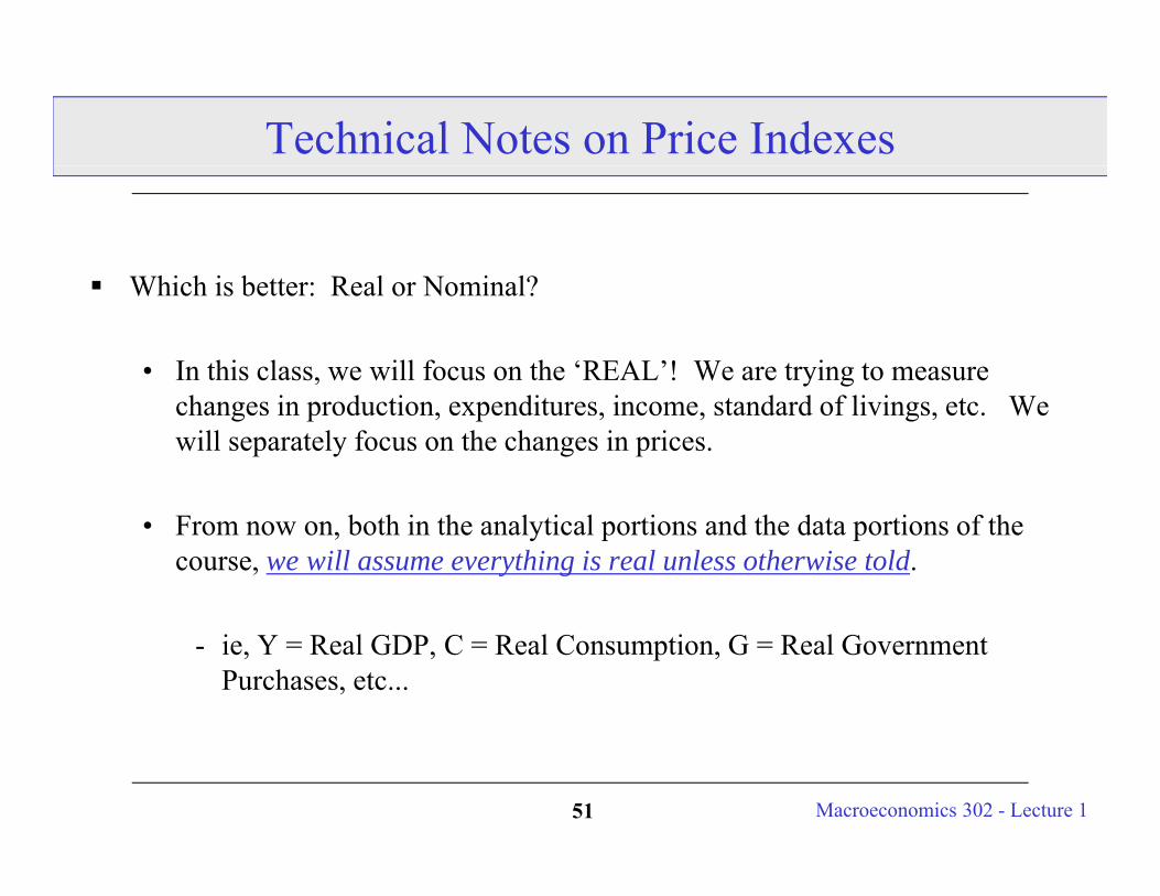
Technical Notes on Price Indexes
Whi h i b tt R l N i l? Which is better: Real or Nominal?
• In this class, we will focus on the ‘REAL’! We are trying to measure changes in production, expenditures, income, standard of livings, etc. We will separately focus on the changes in prices.
• From now on, both in the analytical portions and the data portions of the course, we will assume everything is real unless otherwise told.
- ie, Y = Real GDP, C = Real Consumption, G = Real Government Purchases, etc...
Macroeconomics 302 - Lecture 151

A Look at U.S. Nominal GDP: 1970Q1 – 2006Q3
Black line trend in nominal GDP over time (left axis)
Macroeconomics 302 - Lecture 152
Black line - trend in nominal GDP over time (left axis)Red line - trend in nominal GDP growth (percentage change in nominal GDP) over time(right axis)

A Look at U.S. Inflation 1970M1 - 2006M11
Black line - trend in CPI over time (left axis)Red line - trend in CPI inflation rate (percentage change in CPI) over time(right axis)
Macroeconomics 302 - Lecture 153
( g )Shaded areas represent “official” recession dates (as calculated by NBER)

A Look at U.S. Real GDP 1970Q1 – 2006Q3
Black line - trend in real GDP over time (black axis)Red line - trend in real GDP growth (percentage change in real GDP) over time ( i ht i )
Macroeconomics 302 - Lecture 154
(right axis)Shaded areas represent “official” recession dates (as calculated by National Bureauof Economic Research)

Paul Volcker - Fed Chairman 1979-1987
Macroeconomics 302 - Lecture 155

What is a Recession?
“Un-Official Rule of Thumb” - 2 or more quarters of negative real GDP growth
Most Economies are usually not in recession
• U.S. average postwar expansion: 50 monthsU.S. average postwar expansion: 50 months
• U.S. average postwar recession: 11 months
• Previous Recession: 7 - 9 months (April 2001 – December 2001)
• Previous Expansion: 73 months (Jan 2002- Nov 2007)
• The 1990s experienced the longest expansion since 1850,121 months (more than 10 years; the second longest was 106 months ; 1961-1969.
Macroeconomics 302 - Lecture 156
• For US Business Cycle dates see: www.nber.org/cycles/cyclesmain.html
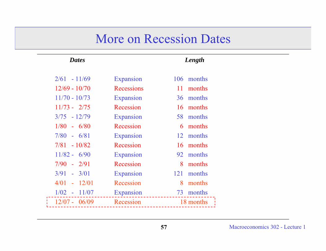
More on Recession DatesDates Length
2/61 11/69 Expansion 106 months2/61 - 11/69 Expansion 106 months12/69 - 10/70 Recessions 11 months11/70 - 10/73 Expansion 36 months11/73 - 2/75 Recession 16 months3/75 - 12/79 Expansion 58 months1/80 - 6/80 Recession 6 months7/80 - 6/81 Expansion 12 months7/81 - 10/82 Recession 16 months11/82 - 6/90 Expansion 92 months7/90 - 2/91 Recession 8 months3/91 3/01 Expansion 121 months3/91 - 3/01 Expansion 121 months 4/01 - 12/01 Recession 8 months1/02 - 11/07 Expansion 73 months12/07 - 06/09 Recession 18 months
Macroeconomics 302 - Lecture 157

More on Recession DatesDates Length
2/61 11/69 Expansion 106 months
49 months of recession in 21
2/61 - 11/69 Expansion 106 months12/69 - 10/70 Recessions 11 months11/70 - 10/73 Expansion 36 months11/73 - 2/75 Recession 16 months 21 years3/75 - 12/79 Expansion 58 months1/80 - 6/80 Recession 6 months7/80 - 6/81 Expansion 12 months
The Great Moderation7/81 - 10/82 Recession 16 months11/82 - 6/90 Expansion 92 months7/90 - 2/91 Recession 8 months3/91 3/01 Expansion 121 months
16 months of recession in27 years
3/91 - 3/01 Expansion 121 months 4/01 - 12/01 Recession 8 months1/02 - 11/07 Expansion 73 months12/07 - 06/09 Recession 18 months
Macroeconomics 302 - Lecture 158
Great Moderation???

Great Moderation!? - Analysis of Real GDP
• Recessions seemed to have become less frequent. Until 2008. • Recent recessions were much less severe than previous recessions. • Even the expansions were more stable Until 2008
Macroeconomics 302 - Lecture 159
• Even the expansions were more stable. Until 2008.• This teaches us a lesson on how hard it is to identify structural breaks in the macroeconomy.

Real GDP and Inflation Over the Last Three Decades?High Inflation: 73-75
79-80
Low Inflation: 82-8396-00 (sustained)02-07 (sustained)
High Growth in GDP: 83-8696-00 (sustained)
Negative Growth in GDP: 74-7579-8081-8290-9190 91
1) Sometimes Negative Growth in GDP and High Inflation (70s)2) Sometimes Negative Growth in GDP and NO High Inflation (80s, 90s, and in 2008-09)
Macroeconomics 302 - Lecture 160
Need Theory to Explain Both Sets of Facts!!!!

Here’s Our Theory: A Brief Overview
We want to learn how GDP, Inflation and Economic Growth are determined.
Economic gro th i th h i GDP ti ( ll l ti i d lik• Economic growth is the change in GDP over time (usually long time periods, like decades or centuries).
• The level of GDP (as opposed to its growth) can determine level of unemployment.• Why do we care about inflation & unemployment?y p y
Questions we will ask:
• Is it possible to have low/stable inflation and high GDP at the same time?• Can too high of a level of GDP be a bad thing?• How can policy makers use the tools available to them to manipulate inflation and
GDP targets?GDP targets?• How do we get sustainable increases in ‘standards of living’ (i.e., economic
growth)?• Specifically, how do workers, firms, consumers, and government agencies interact
Macroeconomics 302 - Lecture 161
to determine macroeconomic outcomes?

Mechanics of the Class
The Demand Side
The aggregate demand (AD) curve represents the expenditure (demand) side of the whole economy.
Aggregate demand curve will relate price changes with changes in ‘real’ expenditures.
Demand side of the economy will be the expenditure side of the economy!y p y
YD = C + I + G + NX (what we learned above)
We will prove later in the course that the AD curve slopes down (take my word for it now). As prices increase, aggregate demand for goods and services in the economy will fall.
Macroeconomics 302 - Lecture 162

The AD Curve: Graphical Representation
Let Y = Real GDPLet P = the aggregate price level (measured by some price index)
P
AD
Y
AD
YThe AD curve need not slope down linearly - it could have some curvature. We willdraw it linearly for simplicity.
Macroeconomics 302 - Lecture 163
The AD curve only shifts when C, I, G, or NX changes.

Mechanics of the Class: Part Deux
The Supply Side
The supply side of the economy is determined by production (what is produced by firms). The focus of Lecture 2 will be on the aggregate production function for the economy.y
• Aggregate Supply (AS) curve is also drawn in the {Y, P} space.• The AS curve will slope up in the short run (we will prove this later in the course, p p ( p ,
the intuition is that if prices go up firms will be more willing to supply goods and services).
• The AS curve will be vertical in the long run at Y* (again, bear with me).
AS will be derived from the aggregate production function:
Macroeconomics 302 - Lecture 164
YS = f(inputs in the economy: land, labor, equipment, machines, oil, etc.).

The AS Curve: Graphical Representations
Let Y = Real GDPLet P = the aggregate price level (measured by some price index)
P Short Run AS
Long Run AS
YY* YThe short-run AS curve is not linearly sloped. We will usually draw it linearly for simplicity. In the real world, the SRAS curve is flatter at lower levels of GDP.The AS curve only shifts when the price of factors of production change (things like
Y
Macroeconomics 302 - Lecture 165
oil prices, wages, and such) or the means of production change (technology) - we will start to model the AS curve in Topic 2.

Potential Output (Y*) - i.e., long-run equilibrium
Potential Output (Y*) is the level of output when the economy is in long-run equilibrium. In other words, if no shocks hit the economy, the economy will stay at Y* (or it will gravitate towards Y*)stay at Y* (or it will gravitate towards Y*).
(ok, that definition is kind of technical, what does Y* really mean?)
Think of it this way, Y* is the level of economic activity that the economy was designed to sustain:
• People are working the ‘right’ amount given labor market conditions (not working too much, not working too little),g g )
• Machines are working the right amount given profit maximizing conditions (not working too much, not working too little)
Macroeconomics 302 - Lecture 166
We will formalize this (and all related concepts) as the course progresses.
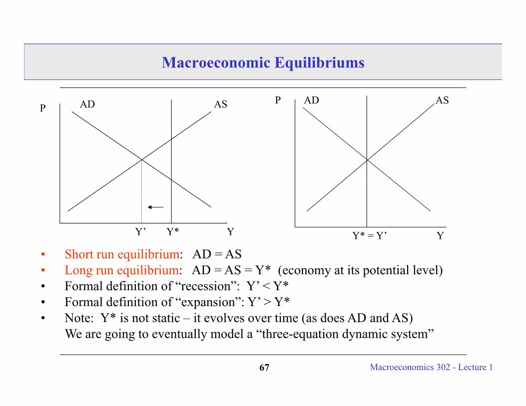
Macroeconomic Equilibriums
PP AD ASAD AS
Y’ Y* YY’ Y* Y Y* = Y’ Y
• Short run equilibrium: AD = AS• Long run equilibrium: AD = AS = Y* (economy at its potential level)• Formal definition of “recession”: Y’ < Y*• Formal definition of “expansion”: Y’ > Y*• Note: Y* is not static – it evolves over time (as does AD and AS)
W i t t ll d l “th ti d i t ”
Macroeconomics 302 - Lecture 167
We are going to eventually model a “three-equation dynamic system”

Macroeconomic Equilibrium
Short-run equilibrium: AD equals short-run AS (SRAS)
What does that mean? What is produced is equal to what is purchased (total expenditures).p )
Long-run equilibrium: AD equals long-run AS (the potential level of output)
What does that mean? What is produced is equal to what is purchased and what is produced is equal to the sustainable level of production.
How are these equilibriums ensured? Prices in the economy adjust (price level, interest rates, wages).
Macroeconomics 302 - Lecture 168

Business Cycles vs. Economic Growth
Business cycle analysis focuses on the movements around Y* (why Y’ differs from Y*)
• Why do we have recessions? Why do we have periods of economic expansions? • Business cycle analysis tends to focus on high-frequency macroeconomic analysis
(quarters, years, maybe a decade)
Economic growth analysis focuses on the evolution of Y* over time.
• Focus is on low-frequency macroeconomic analysis (decades, centuries, etc.)
Y*
Y
timeY’
Y
Macroeconomics 302 - Lecture 169

Congressional Budget Office Estimates Potential Output
Macroeconomics 302 - Lecture 170

Foreshadowing the Rest of the Course: Demand Shocks
The relationship between inflation and output when aggregate demand shifts: Suppose we are in long-run equilibrium at point (a) (AD = SRAS = LRAS)
Short Run AS
Long Run AS
PP
a
bP’P
Y
AD
Y*
AD’
Y’If the economy receives a negative aggregate demand shock, short run equilibriumIf the economy receives a negative aggregate demand shock, short run equilibrium will move from point (a) to point (b). Output will fall (from Y* to Y’). Prices will fall (from P to P’).
D d h k i d t t t i th di ti
Macroeconomics 302 - Lecture 171
Demand shocks cause prices and output to move in the same direction.(You should be able to illustrate a positive demand shock)

Foreshadowing the Rest of the Course: Supply Shocks
The relationship between inflation and output when aggregate supply shifts: Suppose we are in long-run equilibrium at point (a) (AD = SRAS = LRAS)
Short Run AS
Long Run AS
P
Short Run AS’
cP
aP’
P
c
Y
AD
Y*Y’
If the economy receives a negative short-run aggregate supply shock, short run equilibrium will move from point (a) to point (c). Output will fall (from Y* to Y’). Prices will rise (from P to P’).
Macroeconomics 302 - Lecture 172
Supply shocks cause prices and output to move in opposite directions.

Real GDP and Inflation Over the Last Five Decades?
Macroeconomics 302 - Lecture 173
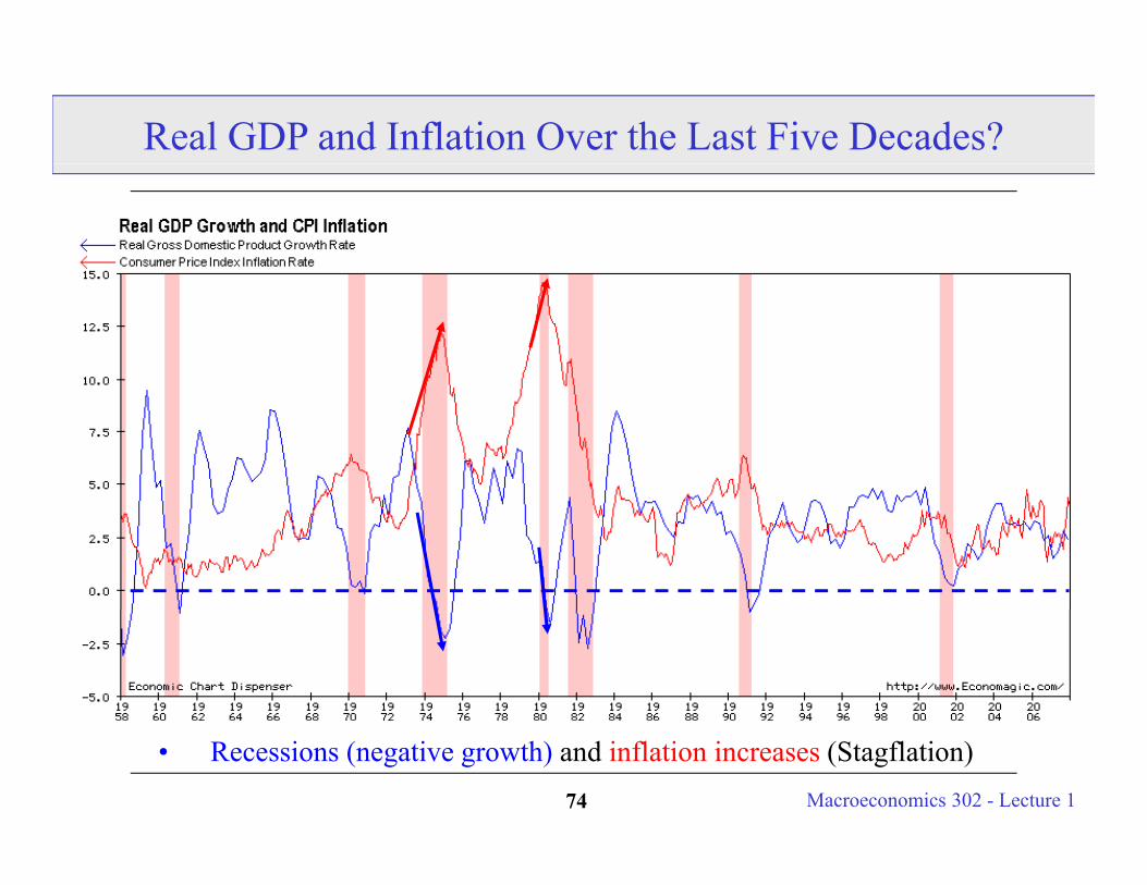
Real GDP and Inflation Over the Last Five Decades?
Macroeconomics 302 - Lecture 174
• Recessions (negative growth) and inflation increases (Stagflation)

Real GDP and Inflation Over the Last Five Decades?
Macroeconomics 302 - Lecture 175
• Recessions (negative growth) and inflation decreases.

Reinterpreting the Business Cycle Data 1970-2001
1970 recessions: Inflation increasing at start of recession! High Increasing Inflation (supply shock)(ca se: rapidl rising oil prices)(cause: rapidly rising oil prices)
1981 recession: Dramatic decrease in inflation at start of recessionNo inflation (demand shock)No inflation (demand shock)(cause: Fed induced recession)
1990 recession: Little increase in inflation/but low level of inflation (demand (shock)(cause: fall in consumer confidence/oil price increase)
R id th i id 1990 N i fl ti ( l h k)Rapid growth in mid 1990s: No inflation (supply shock)(cause: IT revolution)
2001 recession: No inflation (demand shock)
Macroeconomics 302 - Lecture 176
2001 recession: No inflation (demand shock)(cause: over confidence by firms: inventory adjustment)

What’s Next?
Why is inflation bad?
Why is low GDP bad? Why do we care about business cycles?Why is low GDP bad? Why do we care about business cycles?
Th fi l f hi l dd h iThe final part of this lecture addresses these issues.
Macroeconomics 302 - Lecture 177

Interest Rates
i0,1 = the nominal interest rate between periods 0 and 1(the nominal return on the asset)
πe0,1 = the expected inflation rate between periods 0 and 1
re0,1 = the expected real interest rate between periods 0 and 1
D fi i iDefinitions:
re0,1 = i0,1 - πe
0,1 (or i0,1 = πe0,1 + re
0,1)
ra0,1 = i0,1 - πa
0,1 (or i0,1 = πa0,1 + ra
0,1)
Macroeconomics 302 - Lecture 178
where ra and πa are the actual real interest rate and inflation.
Interest Rate Notes
The formula given is approximate. The approximation is less accurate the higher the levels of inflation and nominal interest rates The exact formula is:higher the levels of inflation and nominal interest rates. The exact formula is:
re = (1 + i) / (1 + πe) - 1
Central Banks are very interested in r since it may affect the savings decisionsCentral Banks are very interested in r since it may affect the savings decisions of households and definitely affects the investment decisions of firms. The press talks about Central Banks setting i, but the Central Banks are really trying to set r.
3 easy ways of measuring expected inflation:• Recent actual inflation (see http://www.clev.frb.org).• Survey of forecasters (see http://www.phil.frb.org/econ/liv/welcom.html).• Interest rate spread on nominal vs. inflation-indexed securities (TIPS).
S htt // hil f b / / f/ f ht l f th f t
Macroeconomics 302 - Lecture 179
See http://www.phil.frb.org/econ/spf/spfpage.html for other macro forecasts

Why We Care About Inflation
Inflation is Unpredictable
Indexing Costs (even if you know the inflation rate - you have to deal with it).
Menu Costs (having to go and re-price everything on the shelves/on the menu)Menu Costs (having to go and re price everything on the shelves/on the menu)
Shoe-Leather Costs (you want to hold less cash - have to go to the bank more often)often).
Caveat: There may be some benefits to small inflation rates - more on this later.
Macroeconomics 302 - Lecture 180

Why We Care About Inflation
E l f h i fl ti ff t l t Example of how inflation can affect real returns.
Suppose you and I agree that a real rate of 0.05 over the next year is fair. • borrowing rate, salary growth rate, etc.
Suppose we also agree that expected inflation over the next year is 0.07
We should then set the nominal return equal to 0.12 (i = re + πe)
Summary: i = 0.12re = 0.05
Macroeconomics 302 - Lecture 181
πe = 0.07

Why We Care About Inflation
Suppose that actual inflation is 0.10 (πa > πe)
In this case, ra = 0.02 (ra = i - πa)Borrowers/Firms are better offLenders/Workers worse offLenders/Workers worse off
Suppose that actual inflation is 0.03 (πa < πe)
In this case, ra = 0.09 (ra = i - πa)Borrowers/Firms are worse offL d /W k b ffLenders/Workers better off
Research has also shown that higher inflation rates are correlated with more i bilit P l /Fi D ’t Lik th U t i t
Macroeconomics 302 - Lecture 182
variability. People/Firms Don’t Like the Uncertainty

Measuring Unemployment
Standardized Unemployment Rate:
Labor Force = #Employed + #Unemployed but Looking
Unemployment Rate #Unemployed but Looking/ Labor ForceUnemployment Rate = #Unemployed but Looking/ Labor Force
This is the definition used in most countries, including the U.S.
U.S. data: http://stats.bls.gov/eag.table.htmlU.S. measurement details: http://stats.bls.gov/cps_htgm.htm
Issues: Discouraged Workers, Underemployed, Measurement Issues
Macroeconomics 302 - Lecture 183
Course Pack Reading: 18

Types of Unemployment
F i ti l U l t R lt f M t hi B h i b t Fi d Frictional Unemployment: Result of Matching Behavior between Firms and Workers.
Structural Unemployment: Result of Mismatch of Skills and Employer Needs
Cyclical Unemployment: Result of Output being below full-employment
Is Zero Unemployment a Reasonable Policy Goal?• No! Frictional and Structural Unemployment may be desirable/unavoidable.
Macroeconomics 302 - Lecture 184

Why We Care About Unemployment
Depreciation of Human Capital Depreciation of Human Capital
Productive Externalities Productive Externalities
Social Externalities Social Externalities
I di id l S lf W th Individual Self Worth
Macroeconomics 302 - Lecture 185

The Yield CurveThe Yield Curve
Macroeconomics 302 - Lecture 186

What is a Yield Curve
• A yield curve graphs the interest rate for a given security of differing maturities.
• For example, it represents the yield on 1, 3, 5, 7, and 10 year treasuries.
Historically, yield curves tend to be upward slopingData on U.S. treasury yields from late 2004
Macroeconomics 302 - Lecture 187
Maturity (in years)

Yield Curve Mechanics
Consider a two period model
Define the interest rate on a one year treasury starting today as i0,1
Define the interest rate on a two year treasury starting today as i0,2
What is the relationship between one year treasuries and two year treasuries?What is the relationship between one year treasuries and two year treasuries?
Appeal to theory of arbitrage. If arbitrage holds, then by definition:
(1 + i0,2)2 = (1 + i0,1) * (1 + i1,2)
Macroeconomics 302 - Lecture 188
where i1,2 is the interest rate on a one year treasury starting one period from now.

Shape of the Yield Curve: Macro Explanations
Solve for long interest rates (i0,2) as a function of short rates:
i0,2 = [(1+i0,1) * (1+i1,2)]1/2 – 1
When does the yield curve slope up (i.e., i0,2 > i0,1)? Answer: when i1,2 > i0,1
Remember: i = r + πe (or, with time subscripts, i0,1 = r0,1 + πe0,1)
So, if r is held fixed over time (i.e., r0,1 = r1,2) then the yield curve will slope up if πe
1,2 > πe0,1. Increasing inflation will cause the yield curve to slope up (all
else equal)!else equal)!
Also, if πe is fixed over time (i.e., πe1,2 = πe
0,1) then the yield curve will slope up if r > r Higher f t re real rates ill ca se the ield c r e to slope p (all
Macroeconomics 302 - Lecture 189
if r1,2 > r0,1. Higher future real rates will cause the yield curve to slope up (all else equal).

Revisiting the 2004 Yield Curve?
• Why was the 2004 yield curve sloping upwards? Oil prices were increasing sharply in 2004 which either would put upward pressure on inflation (πe) or
ld lt i th F d fi hti th i fl ti (b i i i) Eithwould result in the Fed fighting the inflation (by raising i). Either way, future short term interest rates would be expected to be higher than currentshort term interest rates (resulting in an upward sloping yield curve).
6 5
7.0
5.5
6.0
6.5
4.5
5.0
Macroeconomics 302 - Lecture 190
4.02 3 4 5 6 7 8 9 10

Flat or Inverted Yield Curves
There is no reason that yield curves need to slope upwards. Expected future short-term rates could be the same or lower than current short-term rates. This would imply that current long rates will be the same or lower than current shortwould imply that current long rates will be the same or lower than current short rates.
This will lead to flat yield curves (current short rates = current long rates) orThis will lead to flat yield curves (current short rates current long rates) or inverted yield curves (current short rates > current long rates).
This possibility could exist in equilibrium! This will occur if inflation isThis possibility could exist in equilibrium! This will occur if inflation is expected to decline over time (or if deflation is predicted) or if future expectations of real interest rates are lower than current real interest rates.
Key: Some people assume that a flat or inverted yield curve means that the economy will be entering a recession! This is not always true. These people are implicitly assuming that we are currently at Y* and a negative demand shock will be occurring in the future (causing either future πe or r to fall)
Macroeconomics 302 - Lecture 191
shock will be occurring in the future (causing either future πe or r to fall).

Example: Yield Curve for U.S. Treasuries
Macroeconomics 302 - Lecture 192Source: US Treasury

Shape of the Yield Curve: Micro Explanations
Our discussion of interest rates was simplified along one dimension – we have ignored risk premiums
i = r + π + ρ (where ρ is the per period risk premium)
Alluding back to our previous discussion, i1,2 > i0,1 if ρ1,2 > ρ0,1
C f i l d d f l i d i Components of ρ include default premiums and term premiums
Declines in ρ for long term assets (i.e., a decline in the term premium) will affect shape of the yield curve.
See an interesting discussion by Ben Bernanke on the shape of yield curves:
Macroeconomics 302 - Lecture 193
g y p yhttp://www.federalreserve.gov/boarddocs/Speeches/2006/20060320/default.htm

Shape of the Yield Curve: Micro Explanations
One component of the term premium: Uncertainty in the future
• If investors are risk averse and the government is risk neutral an• If investors are risk averse and the government is risk neutral, an equilibrium could exist where the government will compensate borrowers for holding longer-term assets.
• A decline in uncertainty (perhaps due to the “Great Moderation” could flatten yield curves relative to historical standards).
A second component of the term premium: Liquidity premium
• If short-term assets are more liquid than long-term assets (or demand for h i l i l hi h h l ) i illshort-term assets is relatively higher than long-term assets), a premium will
exist.
• An increase in the demand for long-term U S assets (perhaps by foreign
Macroeconomics 302 - Lecture 194
An increase in the demand for long term U.S. assets (perhaps by foreign investors) could cause the yield curve to flatten.

Summary Topic 1: What We Have Learned
How GDP, Inflation, Savings, and Unemployment are measured (and problems with their measurement)with their measurement).
The Difference between Real and Nominal Variables.
General Trends in Macro Data over the last few decades.
Any model of the economy we develop should explain the basic facts of the economy!!
Why we care about Inflation and Unemployment.
Th l i bl f th b d ti
Macroeconomics 302 - Lecture 195
The general variables of the economy can be expressed as equations.