interior-point method for nuclear norm approximation...
TRANSCRIPT

Interior-point method for nuclear norm approximation with
application to system identification
Zhang Liu and Lieven Vandenberghe∗
Abstract
The nuclear norm (sum of singular values) of a matrix is often used in convex heuristics forrank minimization problems in control, signal processing, and statistics. Such heuristics can beviewed as extensions of ℓ1-norm minimization techniques for cardinality minimization and sparsesignal estimation. In this paper we consider the problem of minimizing the nuclear norm of anaffine matrix valued function. This problem can be formulated as a semidefinite program, butthe reformulation requires large auxiliary matrix variables, and is expensive to solve by general-purpose interior-point solvers. We show that problem structure in the semidefinite programmingformulation can be exploited to develop more efficient implementations of interior-point methods.In the fast implementation, the cost per iteration is reduced to a quartic function of the problemdimensions, and is comparable to the cost of solving the approximation problem in Frobeniusnorm. In the second part of the paper, the nuclear norm approximation algorithm is applied tosystem identification. A variant of a simple subspace algorithm is presented, in which low-rankmatrix approximations are computed via nuclear norm minimization instead of the singularvalue decomposition. This has the important advantage of preserving linear matrix structurein the low-rank approximation. The method is shown to perform well on publicly availablebenchmark data.
1 Introduction
We discuss the implementation of interior-point algorithms for the nuclear norm approximationproblem
minimize ‖A(x) − B‖∗. (1)
In this problem B ∈ Rp×q is a given matrix,
A(x) = x1A1 + x2A2 + · · · + xnAn
is a linear mapping from Rn to Rp×q, and ‖ · ‖∗ denotes the nuclear norm on Rp×q. (‖X‖∗ isthe sum of the singular values of X, and is also known as the trace norm, the Ky Fan norm, andthe Schatten norm.) The techniques discussed in this paper also apply to problems with an addedconvex quadratic term in the objective,
minimize ‖A(x) − B‖∗ + (x − x0)T Q(x − x0), (2)
∗Electrical Engineering Department, University of California, Los Angeles. Email: [email protected], van-
[email protected]. Research supported by NSF under grants ECS-0524663 and ECCS-0824003, and a Northrop
Grumman Ph.D. fellowship.
1

and nuclear norm approximation problems with convex constraints. However, we will limit mostof the discussion to the unconstrained linear approximation problem for the sake of clarity.
The nuclear norm approximation problem is of interest as a convex heuristic for the rank min-imization problem
minimize rank(A(x) − B),
which is NP-hard in general. The convex nuclear norm heuristic was proposed by Fazel, Hindi,and Boyd [FHB01], and is motivated by the observation that the residual A(x)−B at the optimalsolution of (1) typically has low rank. This idea is very useful for a variety of applications incontrol and system theory, including model reduction, minimum order control synthesis, and systemidentification; see [FHB01, Faz02, FHB04, RFP07]. An important special case is the minimum-rank matrix completion problem, which arises in machine learning [Sre04] and computer vision[TK92, MK97]. In this problem the variables x are the nonzero entries of a sparse matrix A(x); thematrix B has the complementary sparsity pattern and contains the fixed entries in the completionproblem. Another special case is nonnegative factorization, the problem of approximating a matrixby a nonnegative matrix of low rank. This problem arises in data mining [Eld07, §9.2].
The nuclear norm of a diagonal matrix is the ℓ1-norm of the vector formed by its diagonalelements: ‖diag(u)‖∗ = ‖u‖1 for a vector u. The role of the nuclear norm in convex heuristics forrank minimization therefore parallels the use of the ℓ1-norm in sparse approximation or cardinalityminimization [Tib96, HTF01, CDS01, Don06, CT05, CRT06b, CRT06a, Tro06]. The renewedinterest in nuclear norm minimization is motivated by the remarkable success of ℓ1-norm techniquesin practice, and by theoretical results that characterize the possibility of exact recovery of sparsesignals by ℓ1-norm methods [Don06, CT05, CRT06b, CRT06a, Tro06]. Parts of this theoreticalanalysis have recently been extended to nuclear norm methods, providing conditions for exactrecovery of low-rank matrices via nuclear norm optimization [RFP07, CR08, RXH08, CT09, CP09].
Algorithms for nuclear norm approximation This paper is concerned with numerical meth-ods for problem (1), and for extensions of this problem that include convex contraints or regularizedobjectives as in (2). It is well known that the nuclear norm approximation problem can be cast asa semidefinite program (SDP)
minimize (trU + trV )/2
subject to
[
U (A(x) − B)T
A(x) − B V
]
� 0,(3)
with variables x ∈ Rn, U ∈ Sq, V ∈ Sp [FHB01]. (We use Sn to denote the set of symmetricmatrices of order n.) It can therefore be solved by interior-point methods available in general-purpose software for semidefinite programming [Stu99, TTT03, BY05b, YFK03, Bor99]. Interior-point methods offer fast convergence (typically 10-50 iterations), robust performance across differentproblem instances, and high accuracy. However, the memory requirements and the volume ofcomputation per iteration are often high. The SDP (3) has n + p(p + 1)/2 + q(q + 1)/2 variablesand is very difficult to solve by general-purpose solvers, if p and q approach 100. This difficultyhas limited the adoption of nuclear norm methods for rank minimization in practice. The maincontribution of this paper is to describe a more efficient interior-point method that exploits theproblem structure in (3), and is capable of solving problems with dimensions p, q on the order ofseveral hundred.
2

Again, the parallel with ℓ1-norm optimization is instructive. The vector counterpart of prob-lem (1) is the ℓ1-norm approximation problem
minimize ‖Px − q‖1. (4)
This problem can be solved as a linear program (LP)
minimize 1T ysubject to −y � Px − q � y,
(5)
where y is an auxiliary vector variable. Although the LP formulation requires the introduction ofa large number of extra variables, it can be shown that the cost of solving the LP by an interior-point method is comparable to the cost of solving the least-squares counterpart, i.e., to minimizing‖Px − q‖2. To see why, note that an interior-point algorithm typically requires 10–50 iterations,almost independent of the problem size. Each iteration of an interior-point method applied to (5)reduces to solving a set of linear equations
P T DP∆x = r
where D is a positive diagonal matrix with values that change at each iteration [BV04, p. 617]. Thismeans that the cost per iteration of a custom interior-point method for solving (4) is roughly equalto the cost of solving a weighted least-squares problem with coefficient matrix P . In this paper weestablish a similar result for nuclear norm approximation. By exploiting problem structure in theSDP (3), we show that the complexity of an interior-point method can be reduced to O(pqn2) periteration, if n ≥ max{p, q}. This is comparable to solving the norm approximation problem in theleast-squares sense, i.e., to minimizing ‖A(x) − B‖F .
As an alternative to interior-point methods one can consider methods that solve problem (1)directly without requiring the SDP formulation. The cost function f(x) = ‖A(x) − B‖∗ is nondif-ferentiable and convex, and can be minimized by the subgradient method [Sho85]. A subgradient off can be computed from the singular value decomposition (SVD) [RFP07]. Let A(x)−B = PΣQT
be the singular value decomposition of A(x) − B, with P ∈ Rp×r, Σ ∈ Rr×r, and Q ∈ Rq×r,where r is the rank of A(x) − B. Then Aadj(PQT ) is a subgradient of f at x (Aadj is the adjointmapping of A). Since the main computation in each iteration in the subgradient method involvesone singular value decomposition, the time per iteration is lower, and grows more slowly with theproblem dimensions, than one iteration of the interior-point method. However, the convergenceof the subgradient method is often very slow, and the number of iterations to reach an accuratesolution varies widely, depending on the problem data and step size rule.
Another possibility is to replace the cost function with a smooth approximation and thenminimize the smooth approximation by a fast gradient method [Nes04, Nes05, Tse08]. For example,a smooth approximation of the function ‖X‖∗ is obtained by taking the SVD, X =
∑ri=1 σiuiv
Ti ,
replacing the singular values with
hµ(σi) =
{
σ2i /(2µ) σi ≤ µ
σi − µ/2 σi > µ
where µ is a small positive parameter, and defining fµ(X) =∑r
i=1 hµ(σi)uivTi . It can be shown
that
fµ(X) = sup‖Y ‖≤1
(
tr(Y T X) −µ
2‖Y ‖2
F
)
, (6)
3

where ‖Y ‖ denotes the standard matrix norm, i.e., the maximum singular value of Y , and ‖Y ‖F
is the Frobenius norm. Therefore fµ is convex and differentiable, and its gradient is Lipschitzcontinuous with constant 1/µ [HUL93, p.121]. This method applies to much larger problems thanthe interior-point method, but is less accurate (see section 5).
Several algorithms have been proposed for the related problem
minimize ‖X‖∗subject to F(X) = g,
(7)
where F is a linear mapping from Rp×q to Rm, and the optimization variable is X ∈ Rp×q. Oneinteresting approach is to use a factored parametrization X = LRT where L ∈ Rp×r and R ∈ Rq×r.It can be shown that for sufficiently large r, minimizing (‖L‖2
F + ‖R‖2F )/2 subject to F(LRT ) = g,
is equivalent to problem (7) [RFP07]. Thus the problem is transformed to a smooth, nonconvexoptimization problem. This method can be very effective if the rank of the optimal X is small.However it is not guaranteed to find the global optimum.
Recently, a new class of first-order algorithms for the nuclear norm minimization problem (7)has been proposed, extending Bregman iterative algorithms for large-scale ℓ1-norm minimization[MGC, CCS08]. Again each iteration involves a singular value decomposition of X. The complexitycan be further reduced by using an approximate or partial SVD. Although these algorithms wereprimarily developed for the low rank matrix completion problem, they also apply to the generalproblem (7), and are particularly attractive if F and its adjoint are easily evaluated.
Our focus on interior-point methods can be explained by the applications in system identifi-cation that motivated this work. While the optimization problems arising in this context are toolarge for general purpose SDP solvers, they are still orders of magnitude smaller than the machinelearning applications that have inspired the recent work on first-order methods. As mentionedearlier, interior-point methods offer high accuracy and robust performance across different probleminstances. (In particular, we will note that high accuracy is important if the results of the opti-mization are used for model order selection.) Moreover they readily handle variations on the basicproblem format (1), including problems with general convex constraints. As we will see, the capa-bilities of the specialized interior-point method described in the paper are sufficient to investigatethe effectiveness of the nuclear norm heuristic in system identification, an area where it has notbeen widely investigated due to lack of adequate software.
Applications to system identification As a second contribution, we propose and test a sub-space identification algorithm based on quadratically regularized nuclear norm minimization. Thisapproach has important advantages over standard techniques based on the singular value decompo-sition, because it preserves linear (Hankel) structure in low rank approximations. Experiments onbenchmark data sets indicate that the identification method based on nuclear norm minimizationis competitive with existing subspace identification methods in terms of accuracy, and that it cangreatly simplify the selection of the model order.
Outline The paper is organized as follows. In section 2 we review some background on semidefi-nite programming. In section 3.1 we review different semidefinite programming formulations of thenuclear norm approximation problem and give the cost of solving them via general-purpose SDPsolvers. Section 3.2 contains the main result in the paper. We show how standard interior-pointmethods for semidefinite programming can be customized to solve the nuclear norm approximation
4

problem much more efficiently than by general-purpose methods. In section 4 we give numerical ex-periments that illustrate the effectiveness of the method. Section 5 describes in detail applicationsin system identification.
2 Semidefinite programming
This short section provides some necessary background on semidefinite programming.The following optimization problems are Lagrange duals:
(P) minimize tr(CX)subject to G(X) = h
X � 0,
(D) maximize hT zsubject to Gadj(z) � C.
(8)
The variable in the primal problem is a symmetric matrix X ∈ Sn, and the variable in the dualproblem is a vector z ∈ Rm. The coefficients in the cost functions are C ∈ Sn and h ∈ Rm. G is alinear mapping from Sn to Rm, and Gadj is the adjoint of G, i.e., it satisfies uTG(V ) = tr(Gadj(u)V )for all u ∈ Rm, V ∈ Sn. The inequalities denote matrix inequalities. The primal problem is oftencalled an SDP in standard form, and the dual problem an SDP in inequality form.
The most popular methods for solving SDPs are the primal-dual interior-point algorithms. Toestimate the cost of solving the SDPs (8) by a primal-dual interior-point algorithm of the type usedin the popular solvers [Stu99, TTT03], it is sufficient to know that the number of iterations of aninterior-point method is relatively small (usually less than 50) and grows slowly with problem size.Each iteration requires the solution of a set of linear equations
−T−1∆XT−1 + Gadj(∆z) = R, G(∆X) = r
where T ≻ 0. The values of T and the righthand sides R, r change at each iteration. These equationscan be interpreted as linearizations of the nonlinear equations that characterize the primal and dualcentral paths, and are therefore often referred to as the Newton equations.
The Newton equations are solved by eliminating ∆X from the first equation, and then solving
G(TGadj(∆z)T ) = r + G(TRT ) (9)
This is a positive definite set of equations of order m. It can be solved via a Cholesky factorizationif we first express the left hand side as a matrix-vector product H∆z. The cost is O(m3), plus thecost of computing H. The latter part depends on the structure of G, and often exceeds the costof the Cholesky factorization. General-purpose software packages require that G is expressed as avector of inner products
G(X) = (tr(G1X), tr(G2X), . . . , tr(GmX)) . (10)
In this case, the elements of H are given by
Hij = tr(GiTGjT ), i, j = 1, . . . , m. (11)
If no sparsity in the matrices Gi is exploited, this requires O(max{mn3, m2n2}) operations, sinceeach matrix product GiT requires O(n3) operations, and the m2 inner products of tr(GiTGjT )cost O(n2) each.
5
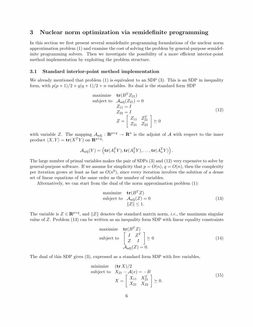
3 Nuclear norm optimization via semidefinite programming
In this section we first present several semidefinite programming formulations of the nuclear normapproximation problem (1) and examine the cost of solving the problem by general-purpose semidef-inite programming solvers. Then we investigate the possibility of a more efficient interior-pointmethod implementation by exploiting the problem structure.
3.1 Standard interior-point method implementation
We already mentioned that problem (1) is equivalent to an SDP (3). This is an SDP in inequalityform, with p(p + 1)/2 + q(q + 1)/2 + n variables. Its dual is the standard form SDP
maximize tr(BT Z21)subject to Aadj(Z21) = 0
Z11 = IZ22 = I
Z =
[
Z11 ZT21
Z21 Z22
]
� 0
(12)
with variable Z. The mapping Aadj : Rp×q → Rn is the adjoint of A with respect to the innerproduct 〈X, Y 〉 = tr(XT Y ) on Rp×q:
Aadj(Y ) =(
tr(AT1 Y ), tr(AT
2 Y ), . . . , tr(ATnY )
)
.
The large number of primal variables makes the pair of SDPs (3) and (12) very expensive to solve bygeneral-purpose software. If we assume for simplicity that p = O(n), q = O(n), then the complexityper iteration grows at least as fast as O(n6), since every iteration involves the solution of a denseset of linear equations of the same order as the number of variables.
Alternatively, we can start from the dual of the norm approximation problem (1):
maximize tr(BT Z)subject to Aadj(Z) = 0
‖Z‖ ≤ 1.(13)
The variable is Z ∈ Rp×q, and ‖Z‖ denotes the standard matrix norm, i.e., the maximum singularvalue of Z. Problem (13) can be written as an inequality form SDP with linear equality constraints
maximize tr(BT Z)
subject to
[
I ZT
Z I
]
� 0
Aadj(Z) = 0.
(14)
The dual of this SDP gives (3), expressed as a standard form SDP with free variables,
minimize (trX)/2subject to X21 −A(x) = −B
X =
[
X11 XT21
X21 X22
]
� 0.(15)
6

We have pq variables in (14), which is less than the number of variables in (3). The secondformulation is therefore recommended when using a general-purpose solver. Nevertheless the costper iteration of a general-purpose method applied to this pair of problems is still very high. If weassume that p = O(n), q = O(n), then the number of variables is still O(n2), and the complexityper iteration grows at least as O(n6).
3.2 Custom interior-point method implementation
We now discuss the possibility of customizing an interior-point method to solve the SDP (3) moreefficiently than by general-purpose solvers. We assume that A has zero nullspace (i.e., the coefficientmatrices Ai are linearly independent) and that p ≥ q (since otherwise we can minimize ‖A(x)T −BT ‖∗).
The key step in each iteration of an interior-point method based on primal or dual scalingdirections, or on the Nesterov-Todd primal-dual scaling direction [NT97, TTT98], is the solutionof a set of linear equations
Aadj(∆Z) = r,
[
∆U A(∆x)T
A(∆x) ∆V
]
+ T
[
0 ∆ZT
∆Z 0
]
T = R (16)
to compute search directions ∆x, ∆U , ∆V , ∆Z. The matrices
T =
[
T11 T T21
T21 T22
]
∈ Sp+q, R =
[
R11 RT21
R21 R22
]
∈ Sp+q,
and the vector r ∈ Rn are given, with T11 ∈ Sq, R11 ∈ Sq. The matrix T is positive definite.It is clear that if we know ∆Z and ∆x in (16), then ∆U and ∆V follow from
∆U = R11 − T11∆ZT T21 − T T21∆ZT11, ∆V = R22 − T21∆ZT T22 − T22∆ZT T
21. (17)
We can therefore focus on the reduced equations
Aadj(∆Z) = r, A(∆x) + T22∆ZT11 + T21∆ZT T21 = R21, (18)
with variables ∆x ∈ Rn, ∆Z ∈ Rp×q. To simplify (18), we start by computing a block-diagonalcongruence transformation that reduces the four blocks of T to diagonal form:
[
W1 00 W2
] [
T11 T T21
T21 T22
] [
W T1 0
0 W T2
]
=
[
I ΣT
Σ I
]
, Σ =
[
diag(σ1, . . . , σq)0
]
with 0 ≤ σk < 1, k = 1, . . . , q. The matrices W1 and W2 can be computed as
W1 = QT L−11 , W2 = P T L−1
2 ,
where L1 and L2 are Cholesky factors of T11 = L1LT1 and T22 = L2L
T2 , and the orthogonal
matrices P ∈ Rp×p, Q ∈ Rq×q and the diagonal matrix Σ ∈ Rp×q follow from the singular valuedecomposition
L−12 T21L
−T1 = PΣQT .
7

If we now define ∆Z = W−T2 ∆ZW−1
1 , A(·) = W2A(·)W T1 , and R21 = W2R21W
T1 , then the equa-
tions (18) reduce to
Aadj(∆Z) = r, A(∆x) + ∆Z + Σ∆ZT Σ = R21. (19)
This has the same form as (18), but with T11 and T22 replaced with identity matrices, and T21 witha positive diagonal matrix. It is important to note that the singular values σk are less than one, asa consequence of the positive definiteness of T .
The diagonal structure in (19) makes it easy to eliminate ∆Z. To see this, consider the mapping
S : Rp×q → Rp×q, S(X) = X + ΣXT Σ.
The mapping S is self-adjoint and positive definite, and can be factored as
S(X) = L(Ladj(X)), (20)
where L : Rp×q → Rp×q is defined by
L(X)ij =
√
1 − σ2i σ
2j Xij + σiσjXji i < j
√
1 + σ2i Xii i = j
Xij i > j,
and its adjoint Ladj : Rp×q → Rp×q by
Ladj(X)ij =
Xij i > qXij + σiσjXji q ≥ i > j√
1 + σ2i Xii i = j
√
1 − σ2i σ
2j Xij i < j.
Note that L is lower-triangular when represented as a pq×pq matrix that maps vec(X) (the matrixX stored in column major order as a pq-vector) to vec(L(X)). The factorization (20) can thereforebe interpreted as a Cholesky factorization of S. The inverse mappings of L and its adjoint are
L−1(X)ij =
(Xij − σiσjXji)/√
1 − σ2i σ
2j i < j
Xii/√
1 + σ2i i = j
Xij i > j
and
L−1adj(X)ij =
Xij i > q
Xij − σiσjXji/√
1 − σ2i σ
2j q ≥ i > j
Xii/√
1 + σ2i i = j
Xij/√
1 − σ2i σ
2j i < j.
These expressions provide O(q2) algorithms for evaluating S and its inverse.Returning to (19), we can use the second equation to express ∆Z in terms of ∆x as
∆Z = S−1(R21 − A(∆x)). (21)
8

Substituting this in the first equation gives an equation in ∆x:
H∆x = g (22)
where g = Aadj(S−1(R21))− r and H is the matrix that satisfies H∆x = Aadj(S
−1(A(∆x))) for all∆x, i.e.,
Hij = tr(ATi S
−1(Aj)) = tr(L−1(Ai)TL−1(Aj)), i, j = 1, . . . , n, (23)
Since A has full rank and S is positive definite, (22) is a positive definite set of linear equations.After solving for ∆x, we first obtain ∆Z and ∆Z = W T
2 ∆ZW1 from (21), and then ∆U , ∆Vfrom (17).
Several methods can be used to solve (22). We can compute the matrix H by computingL−1(Ai)) for i = 1, . . . , n and forming the inner products (23), and then factor H using a Choleskyfactorization. Another method is to note that H = GT G, where
G =[
vec(L−1(A1)) vec(L−1(A2)) · · · vec(L−1(An)))]
.
We can therefore use a QR factorization of G to factor H. This is slower (by a factor of at most two)than the Cholesky factorization method and requires more memory. However it is also numericallymore stable because it allows us to compute a triangular factorization of the matrix H withoutexplicitly calculating H.
Complexity The linear algebra complexity per iteration of the custom interior-point algorithmcan be estimated as follows. The cost of computing the congruence transformation W and thesingular value matrix Σ is O(p3) (recall our assumption that p ≥ q). The cost of computing thecoefficients of the scaled mapping
A(x) = x1A1 + x2A2 + · · · + xnAn,
i.e., computing Ai = W2AiWT1 for i = 1, . . . , n, is O(np2q) if the coefficient matrices Ai are dense
and unstructured. Solving (22) by Cholesky factorization or QR factorization costs O(n2pq) (recallour assumption that the A has zero nullspace, and hence n ≤ pq). If we make the reasonableassumption that n ≥ p, we see that the overal cost is O(n2pq). If the coefficient matrices Ai aredense, this is comparable to solving the linear norm approximation problem in the Frobenius norm,i.e., solving a least squares problem with n variables and pq equations. More generally, if p = O(n),q = O(n), the cost per iteration increases as O(n4), as opposed to O(n6) if we use general-purposesoftware.
4 Numerical experiments
4.1 Randomly generated problems
We first consider a family of randomly generated nuclear norm approximation problems (1) withn = p = q. The matrices Ai and B have entries independently generated from N (0, 1). Thenumber of variables n ranges from 20 to 350. Table 1 shows the time per iteration in seconds on a3.0 GHz processor with 3 GB of memory. A graph of the results is shown in Figure 1. All timesare averaged over five randomly generated instances. The number of iterations ranges from 8 to
9

n SeDuMi SDPT3 CVXOPT
20 0.25 0.29 0.0350 13 4.0 0.1575 138 33 0.34100 0.93150 2.7200 8.3275 23350 50
Table 1: Time per iteration in seconds for two standard SDP solvers and a custom interior-pointmethod, for randomly generated problems with n = p = q.
101
102
10310
-2
10-1
100
101
102
103
SeDuMiSDPT3CVXOPT
Problem dimension n
Tim
eper
iter
atio
n(s
econ
ds)
Figure 1: Graph of the results in table 1.
10

15 for all experiments. Blank entries in the table indicate that the simulation was aborted dueto memory limitations. Columns 2 and 3 show the statistics for solving the problem using thegeneral-purpose solvers SeDuMi (version 1.1R3) [Stu99] and SDPT3 (version 4.0 beta) [TTT03] inMatlab (version R2007a). The last column shows the results of a custom implementation of thealgorithm described in Section 3.2 using CVXOPT (version 1.0) [DV08]. CVXOPT is written inPython (version 2.5), with critical linear algebra computations implemented in C using LAPACK(version 3.1.1) and ATLAS (version 3.8.1). It includes an SDP solver that can be customized byproviding functions to evaluate the constraints and to solve the Newton equations.
The results clearly illustrate the effectiveness of the fast algorithm of Section 3.2 in comparisonwith general-purpose solvers. Within the range of problem sizes considered here, the times periteration grow roughly as n5 for the general purpose solvers, and as n3 for the custom solvers. Forlarger problem sizes, the times per iteration can be expected to increase as n6, respectively, n4, aspredicted by the flop count analysis at the end of section 3.2.
4.2 An open-loop control problem
The second experiment is a variation on an example from [FHB04]. The problem is to design a low-order discrete-time controller for a plant, so that the step response of the combined controller andplant lies within specified bounds. We denote the plant impulse response by h(t), t = 0, . . . , N , thecontroller impulse response by x(t), t = 0, . . . , N , and the step input by u(t) = 1 for t = 0, . . . , N .The impulse response coefficients x(t) are the variables in the problem, and are computed by solvingthe convex optimization problem
minimize ‖H(x)‖∗subject to bl(t) ≤ (h ∗ x ∗ u)(t) ≤ bu(t), t = 0, . . . , N,
(24)
where bl and bu are given lower and upper bounds on the step response, ∗ denotes convolution, and
H(x) =
x(1) x(2) x(3) · · · x(N)x(2) x(3) x(4) · · · x(N + 1)
......
......
x(N) x(N + 1) x(N + 2) · · · x(2N − 1)
.
The variables are x(t), t = 0, . . . , 2N − 1.Figure 2 shows the result for a 6th-order plant with transfer function
P (z) =0.0158z5 − 0.00292z4 − 0.0284z3 + 0.0177z2 + 0.00816z − 0.00828
z6 − 4.03z5 + 7.4z4 − 8.06z3 + 5.57z2 − 2.31z + 0.434,
and N = 160. The step response of the original system has a long rise time and large biased steadystate error. After solving the optimization problem (24), we obtain a second-order controller withtransfer function
X(z) =1.58z2 − 3.06z + 1.48
z2 − 1.93z + 0.931.
The step response with the low-order controller satisfies all the time-domain constraints as shownin the figure. The singular values of H(x∗) at the optimal solution x∗ are plotted in Figure 3, whichclearly shows H(x∗) has rank 2.
11

0 2 4 6 8 10 12 14 16−0.2
0
0.2
0.4
0.6
0.8
1
1.2
Without controller
With controller
Upper/lower bound
Time (seconds)
Ste
pre
spon
se
Figure 2: Open-loop controller design with time-domain constraints.
0 2 4 6 8 10 12 14 16 18 2010
−12
10−10
10−8
10−6
10−4
10−2
100
Singular value index
Sin
gula
rva
lue
Figure 3: Largest singular values of the Hankel matrix H(x∗) at the optimal solution x∗ of theopen-loop controller design example.
12

The dimensions of the optimization (24) are p = 160, q = 160, n = 320, so the resulting SDP hasmore than 25000 variables. The custom interior-point method implemented in CVXOPT, reducesthe relative duality gap and relative primal and dual residual below 10−6 in 15 iterations, and takesless than 2 minutes on a 3.0 GHz processor.
5 Application to system identification
In this section we present a system identification method based on nuclear norm minimization. Theobjective is to fit a discrete-time linear time-invariant state-space model
x(t + 1) = Ax(t) + Bu(t), y(t) = Cx(t) + Du(t), (25)
to a sequence of inputs u(t) ∈ Rm and outputs y(t) ∈ Rp, t = 0, . . . , N . The vector x(t) ∈ Rn
denotes the state of the system at time t, and n is the order of the system model. The parametersto be estimated are the model order n, the matrices A, B, C, D, and the initial state x(0).
Subspace algorithms [Lar90, Ver94, OD94, Vib95] use the singular value decomposition (SVD)of matrices constructed from observed inputs and outputs to estimate the system order, and tocompute low-rank approximations from which the model parameters are subsequently determined.Nuclear norm minimization offers an alternative method for computing low rank matrix approxi-mations. An advantage of this approach is that the matrix structure (for example, the block Hankelstructure common in subspace identification) can be taken into account before the rank or modelorder is chosen. As a consequence the minimum nuclear norm approximation typically provides amore clear-cut criterion for model selection than the SVD low-rank approximation.
5.1 Input-output equation
Suppose we are given a sequence of inputs and outputs u(t), y(t), t = 0, . . . , N . If we define blockHankel matrices
Y =
y(0) y(1) y(2) · · · y(N − r)y(1) y(2) y(3) · · · y(N − r + 1)
......
......
y(r) y(r + 1) y(r + 2) · · · y(N)
and
U =
u(0) u(1) u(2) · · · u(N − r)u(1) u(2) u(3) · · · u(N − r + 1)
......
......
u(r) u(r + 1) u(r + 2) · · · u(N)
,
we obtain from (25) the equationY = GX + HU (26)
where
G =
CCACA2
...CAr
, H =
D 0 0 · · · 0CB D 0 · · · 0
CAB CB D · · · 0...
......
. . ....
CAr−1B CAr−2B CAr−1B · · · D
,
13
andX =
[
x(0) x(1) x(2) · · · x(N − r)]
.
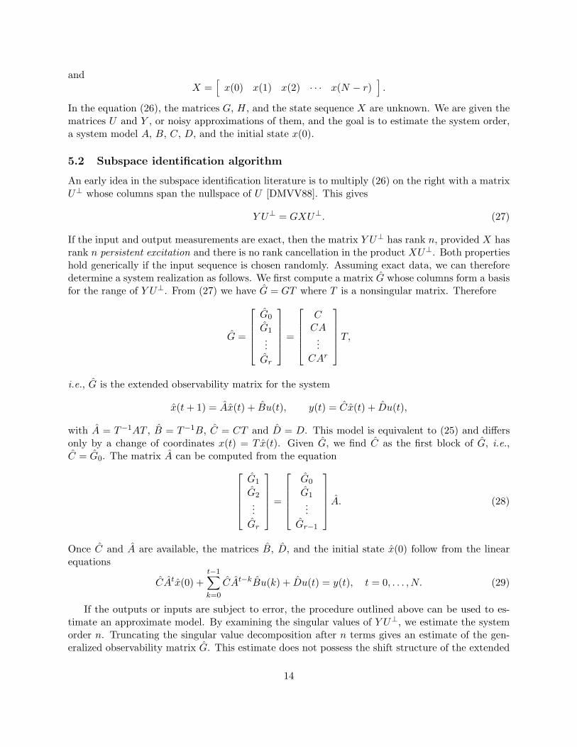
In the equation (26), the matrices G, H, and the state sequence X are unknown. We are given thematrices U and Y , or noisy approximations of them, and the goal is to estimate the system order,a system model A, B, C, D, and the initial state x(0).
5.2 Subspace identification algorithm
An early idea in the subspace identification literature is to multiply (26) on the right with a matrixU⊥ whose columns span the nullspace of U [DMVV88]. This gives
Y U⊥ = GXU⊥. (27)
If the input and output measurements are exact, then the matrix Y U⊥ has rank n, provided X hasrank n persistent excitation and there is no rank cancellation in the product XU⊥. Both propertieshold generically if the input sequence is chosen randomly. Assuming exact data, we can thereforedetermine a system realization as follows. We first compute a matrix G whose columns form a basisfor the range of Y U⊥. From (27) we have G = GT where T is a nonsingular matrix. Therefore
G =
G0
G1...
Gr
=
CCA...
CAr
T,
i.e., G is the extended observability matrix for the system
x(t + 1) = Ax(t) + Bu(t), y(t) = Cx(t) + Du(t),
with A = T−1AT , B = T−1B, C = CT and D = D. This model is equivalent to (25) and differsonly by a change of coordinates x(t) = T x(t). Given G, we find C as the first block of G, i.e.,C = G0. The matrix A can be computed from the equation
G1
G2...
Gr
=
G0
G1...
Gr−1
A. (28)
Once C and A are available, the matrices B, D, and the initial state x(0) follow from the linearequations
CAtx(0) +t−1∑
k=0
CAt−kBu(k) + Du(t) = y(t), t = 0, . . . , N. (29)
If the outputs or inputs are subject to error, the procedure outlined above can be used to es-timate an approximate model. By examining the singular values of Y U⊥, we estimate the systemorder n. Truncating the singular value decomposition after n terms gives an estimate of the gen-eralized observability matrix G. This estimate does not possess the shift structure of the extended
14

observability matrix, so the overdetermined set of equations (28) is not solvable. As an approximatesolution we can take C = G0, and compute a least-squares solution A to (28). Similarly, we cancompute a least-squares solution of the overdetermined set of equations (29) to find estimates B,D and x(0). We refer to [Lju99, Section 10.6] for more details.
5.3 Identification by nuclear norm optimization
We now present a variation on the algorithm of the previous section based on nuclear norm mini-mization. We will use y(t), t = 0, . . . , N , as optimization variables, and distinguish the computedoutputs y(t) from the given measurements ymeas(t). As before, the matrix Y will denote the Hankelmatrix constructed from y(t). The proposed method is based on computing y(t) by solving theconvex optimization problem
minimize ‖Y U⊥‖∗ + γN∑
t=0
‖y(t) − ymeas(t))‖22 , (30)
for a positive weighting parameter γ. This gives a point on the trade-off curve between the nuclearnorm of Y U⊥ (as a proxy for rank(Y U⊥)), and the deviation between the sequences y(t) andymeas(t). From the optimal solution y(t) of (30), we can compute the singular value decompositionof Y U⊥, and proceed as in the method of section 5.2.
Obviously, many variations on this idea exist. For example, we can move the deviation betweenmeasured and computed output to the constraints, and solve
minimize ‖Y U⊥‖∗subject to ‖y(t) − ymeas(t)‖ ≤ ǫ, t = 0, . . . , N.
We can also use a weighted norm to measure the deviation, as in
minimize ‖Y U⊥‖∗ +N∑
t=0
‖Wt(y(t) − ymeas(t))‖22 .
The method can also be extended to cases where the inputs are subject to error.The idea outlined above is related to subspace algorithms based on structured total least squares
[MWV+05, De 94]. In these methods a low rank constraint on a structured matrix A(x) is imposedvia nonlinear equality constraints A(x)y = 0, yT y = 1. The resulting nonconvex optimizationproblem is solved locally via nonlinear optimization.
5.4 Experimental results
We have implemented the algorithm proposed in section 5.3 and tested it on ten benchmark prob-lems from the Daisy collection [DDDF97]. A brief description of the data sets is given in table 2.NI is the number of data points used in the identification experiment, and NV is the number ofdata points that will be used for model validation. This includes the NI data points used in theidentification.
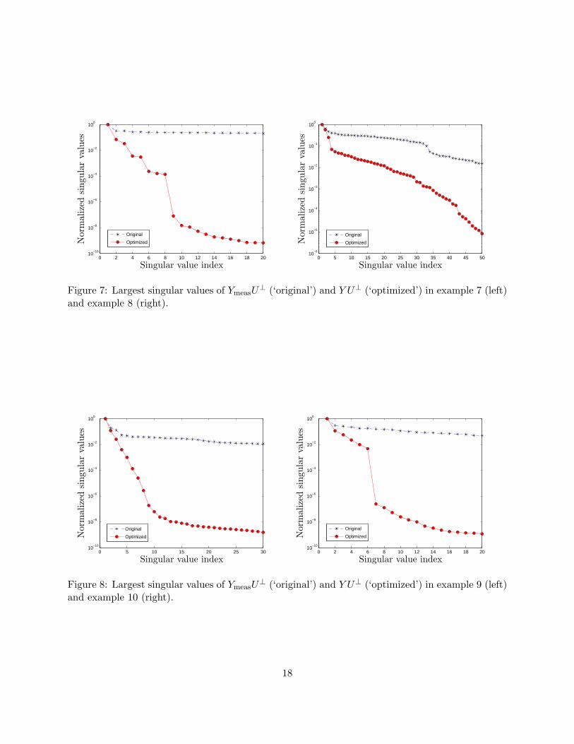
We first apply the method of section 5.3, based on the nuclear norm minimization problem (30).Figures 4–8 show the singular values of Y U⊥ for the ten examples, where Y is the solution of theoptimization problem (30) with N = NI . The parameter γ was selected by examining different
15

Data set Description Inputs Outputs NI NV
1 96-007 CD player arm 2 2 200 6002 98-002 Continuous stirring tank reactor 1 2 250 7003 96-006 Hair dryer 1 1 150 4004 97-002 Steam heat exchanger 1 1 400 10005 99-001 SISO heating system 1 1 400 8006 96-009 Flexible robot arm 1 1 100 3007 96-011 Heat flow density 2 1 400 10008 97-003 Industrial winding process 5 2 250 6009 96-002 Glass furnace 3 6 150 40010 96-016 Industrial dryer 3 3 250 600
Table 2: Ten benchmark problems from the Daisy collection [DDDF97]. NI is the number of datapoints that will be used in the identification experiment. NV is the number of points used forvalidation.
0 2 4 6 8 10 12 14 16 18 2010
−10
10−8
10−6
10−4
10−2
100
Original
Optimized
Singular value index
Nor
mal
ized
singu
lar
valu
es
0 2 4 6 8 10 12 14 16 18 2010
−10
10−8
10−6
10−4
10−2
100
Original
Optimized
Singular value index
Nor
mal
ized
singu
lar
valu
es
Figure 4: Largest singular values of YmeasU⊥ (‘original’) and Y U⊥ (‘optimized’) in example 1
(left) and example 2 (right). Ymeas and U are block-Hankel matrices constructed from the input-output data. Y is a block-Hankel matrix constructed from the optimal solution of the optimizationproblem (30).
16

0 2 4 6 8 10 12 14 16 18 2010
−10
10−8
10−6
10−4
10−2
100
Original
Optimized
Singular value index
Nor
mal
ized
singu
lar
valu
es
0 2 4 6 8 10 12 14 16 18 2010
−10
10−8
10−6
10−4
10−2
100
Original
Optimized
Singular value index
Nor
mal
ized
singu
lar
valu
esFigure 5: Largest singular values of YmeasU
⊥ (‘original’) and Y U⊥ (‘optimized’) in example 3 (left)and example 4 (right).
0 2 4 6 8 10 12 14 16 18 2010
−10
10−8
10−6
10−4
10−2
100
Original
Optimized
Singular value index
Nor
mal
ized
singu
lar
valu
es
0 2 4 6 8 10 12 14 16 18 2010
−7
10−6
10−5
10−4
10−3
10−2
10−1
100
Original
Optimized
Singular value index
Nor
mal
ized
singu
lar
valu
es
Figure 6: Largest singular values of YmeasU⊥ (‘original’) and Y U⊥ (‘optimized’) in example 5 (left)
and example 6 (right).
17
0 2 4 6 8 10 12 14 16 18 2010
−10
10−8
10−6
10−4
10−2
100
Original
Optimized
Singular value index
Nor
mal
ized
singu
lar
valu
es
0 5 10 15 20 25 30 35 40 45 5010
−6
10−5
10−4
10−3
10−2
10−1
100
Original
Optimized
Singular value index
Nor
mal
ized
singu
lar
valu
esFigure 7: Largest singular values of YmeasU
⊥ (‘original’) and Y U⊥ (‘optimized’) in example 7 (left)and example 8 (right).
0 5 10 15 20 25 3010
−10
10−8
10−6
10−4
10−2
100
Original
Optimized
Singular value index
Nor
mal
ized
singu
lar
valu
es
0 2 4 6 8 10 12 14 16 18 2010
−10
10−8
10−6
10−4
10−2
100
Original
Optimized
Singular value index
Nor
mal
ized
singu
lar
valu
es
Figure 8: Largest singular values of YmeasU⊥ (‘original’) and Y U⊥ (‘optimized’) in example 9 (left)
and example 10 (right).
18

Nuclear norm method N4SID default N4SIDn eI eV n eI eV n eI eV
1 3 0.17 0.18 10 0.15 0.24 3 0.16 0.192 3 0.23 0.23 7 0.22 0.20 3 0.26 0.233 4 0.069 0.12 3 0.079 0.13 4 0.080 0.134 6 0.12 0.20 2 0.21 0.47 6 0.22 0.385 4 0.02 0.085 2 0.038 0.094 4 0.032 0.0906 4 0.028 0.038 7 0.046 0.075 4 0.13 0.267 8 0.14 0.14 1 0.18 0.17 8 0.14 0.138 3 0.17 0.17 10 0.17 0.18 3 0.18 0.179 5 0.21 0.36 10 0.31 0.47 5 0.54 0.5910 6 0.28 0.27 10 0.31 0.32 6 0.37 0.26
Table 3: Identification results for the ten benchmark problems. For each of the three methods, n isthe estimated system order, eI is the relative estimation error on the identification data, and eV isthe relative prediction error on the validation data. ‘Nuclear norm method’ refers to the algorithmdescribed in section 5.3. The results under ‘N4SID default’ were obtained by the Matlab commandn4sid with default values of the parameters. The results under ‘N4SID’ were obtained by n4sid
with a specified model order.
points on the trade-off curve, and choosing the value that gives approximately the smallest valueof identification error. The singular values are normalized so that the largest singular value is one.As can be seen, in most cases the nuclear norm optimization provides a Hankel matrix Y withY U⊥ very close to low rank, and the singular value plots suggest a distinct value for the modelorder. When this is not the case (as in example 9), we take n equal to the number of singularvalues greater than 10−3 times the first singular value. The figures also show the singular valuesof YmeasU
⊥, where Ymeas is the Hankel matrix constructed from the output data. These singularvalues typically do not indicate a clear choice for the model order.
Columns 2–4 of table 3 summarize the results of the identification based on the nuclear normapproximation. n is the estimated system order. eI and eV are the identification error and validationerror, computed as
eI =
(
∑NI−1t=0 ‖ymeas(t) − y(t)‖2
2∑NI−1
t=0 ‖ymeas(t) − yI‖22
)1/2
, eV =
(
∑NV −1t=0 ‖ymeas(t) − y(t)‖2
2∑NV −1
t=0 ‖ymeas(t) − yV ‖22
)1/2
, (31)
respectively, where ymeas(t) are the given output data,
yI =1
NI
NI−1∑
t=0
ymeas(t), yV =1
NV
NV −1∑
t=0
ymeas(t),
and y(t) is the output of the identified state-space model, starting at the estimated initial state. Intable 3 we also give the results obtained with the subspace identification algorithm implemented inthe Matlab Identification Toolbox. The results under ‘N4SID default’ are for the models computedby the Matlab command n4sid with the default settings (including the feedthrough matrix D).The results under ‘N4SID’ are from n4sid with a specified model order, equal to the order used inthe nuclear norm method. We note that the identification errors for the nuclear norm optimization
19

10−3
10−2
10−1
100
101
0.08
0.1
0.12
0.14
0.16
0.18
0.2
0.22
0.24
Identification
Validation
Nuclear norm
Iden
tifica
tion
and
validat
ion
erro
r
Figure 9: Trade-off between the identification/validation error (eI/eV ) and the nuclear norm‖Y U⊥‖∗ in example 1.
algorithm are comparable or slightly lower than n4sid. The main advantage of the nuclear normtechnique appears to be that it makes the selection of an appropriate model order easier.
Figures 9 and Figure 10 provide some further illustration of the identification algorithm. Fig-ure 9 shows the trade-off between the identification/validation error (eI/eV ) and the nuclear normof Y U⊥, for the first example. The trade-off curves were computed by solving problem (30) fora range of different values of γ. eI and eV are calculated using (31) based on the predictions ofthe identified state-space model. In Figure 10 we compare the measured outputs with the modelpredictions for example 1. The first NI = 200 points were used for the identification.
5.5 Comparison with first-order method
In this section we compare the speed and accuracy of the interior-point method with a first-ordermethod. We use Nesterov’s optimal gradient method of 1983 [Tse08, Algorithm 2] to minimize asmooth approximation of the problem (30), obtained by replacing the nuclear norm by the smoothmatrix function (6). The problem data are from example 1, and the problem dimensions are p = 81,q = 80, and n = 400. We use three different values of the smoothing parameter µ, and a fixed stepsize t in the gradient steps (selected for best performance by trial and error).
The left plot in Figure 11 shows the relative accuracy versus the number of iterations. Therelative error in this plot refers to the original, nonsmooth problem, i.e., it is defined as (f (k) −f⋆)/f⋆, where f (k) is the objective value of (30) after k iterations and f∗ is the optimal value. (Thisexplains why the error levels off at a relatively high value.) For the same problem, the interior-point method reaches an accurate solution in ten iterations. However the average CPU time periteration of the interior-point method is 2.4 seconds, and is much larger than the 0.02 seconds of the
20

0 100 200 300 400 500 600−2
−1
0
1
2
0 100 200 300 400 500 600−2
−1
0
1
2
Measured
Identified
Time
Time
Outp
ut
1O
utp
ut
2
Figure 10: Measured and identified outputs in example 1.
0 2000 4000 6000 8000 10000 1200010
−4
10−3
10−2
10−1
100
101
102
µ=1e−2, t=3e−4
µ=1e−3, t=3e−5
µ=1e−4, t=3e−6
Number of iterations
Rel
ativ
eer
ror
100
101
102
10−8
10−6
10−4
10−2
100
102
µ=1e−2, t=3e−4
µ=1e−3, t=3e−5
µ=1e−4, t=3e−6
Interior method
Rel
ativ
eer
ror
CPU time in seconds
Figure 11: Convergence of interior-point method and a fast gradient method applied to a smoothapproximation, with smoothing parameter µ. The parameter t is the step size in the gradientmethod.
21

0 5 10 15 2010
−10
10−8
10−6
10−4
10−2
100
µ=1e−2, t=3e−4
µ=1e−3, t=3e−5
µ=1e−4, t=3e−6
Interior method
Singular value index
Nor
mal
ized
singu
lar
valu
es
Figure 12: Normalized singular values from the fast gradient method and interior-point method.
gradient method. The right plot in Figure 11 shows the relative accuracy versus elapsed CPU time.The figure shows that when µ is sufficiently large, the first-order method can reach a moderateaccuracy faster than the interior-point method. For larger problems, the difference will be evenmore pronounced. Figure 12 shows the singular values of the solutions for each value of µ. Here wenote that the gap between zero and nonzero singular values rapidly decreases when the smoothingis increased. In combination, these three plots illustrate the trade-off between the quality of thesmooth approximation and the complexity of solving it. The experiment also demonstrates theimportance of the robustness and high accuracy of interior-point methods when the results of thenuclear norm minimization are used for model order selection.
6 Conclusion
We have described techniques for improving the efficiency of interior-point methods for nuclearnorm approximation. By exploiting problem structure in the linear equations that form the mostexpensive part of an interior-point method, we were able to reduce the cost per iteration to O(n2pq)operations, where n is the number of variables, p and q are the matrix dimensions, and we assumethat n ≥ max{p, q}. The techniques can be used in combination with standard primal-dual interior-point algorithms of the type implemented in the general-purpose solvers SDPT3 and Sedumi. Thisresults in algorithms with the same robustness and high accuracy as the state-of-the-art SDP solvers,but with a much lower computational cost. The cost can be further reduced by exploiting structurein the mapping A(x). For example, some of the techniques developed for linear matrix inequalitieswith Hankel and Toeplitz structure in [GHNV03, RV06] extend to the problem considered here.
As an application, we implemented and tested a subspace algorithm for system identificationbased on nuclear norm approximation. The experimental results on benchmark data sets suggestthat the quality of the models obtained by this method is comparable with state-of-the-art subspaceidentification software. An important advantage of the nuclear norm method for computing low
22

rank approximations is that, unlike the SVD, it preserves linear matrix structure. It also providesa less equivocal criterion for the selection of the system order.
We have not discussed the implementation of interior-point methods for the least-norm prob-lem (7) or its SDP formulation
minimize (trU + trV )/2
subject to
[
U XT
X V
]
� 0
F(X) = g.
(32)
This SDP includes extra matrix variables U , V , and is therefore also very expensive to solvevia general-purpose solvers. However the steps required for a custom implementation are morestraightforward than for the nuclear norm approximation problem considered in the paper. TheNewton equations for (32) take the form
T
[
0 Fadj(∆z)T
Fadj(∆z) 0
]
T −
[
∆U ∆XT
∆X ∆V
]
=
[
R11 RT21
R21 R22
]
, F(∆X) = r,
where
T =
[
T11 T12
T21 T22
]
is a positive definite scaling matrix. By eliminating ∆U , ∆V , ∆X from the first equation we obtaina smaller (and usually dense) system H∆z = r where H is the matrix defined by
Hu = F(
T22Fadj(u)T11 + T21Fadj(u)T T21
)
.
The key to improving the efficiency is then to exploit structure in F when assembling the matrixH. Properties that can be exploited are sparsity or low rank-structure (in the coefficients Fi, if weexpress F as F(X) = (tr(F T
1 X), . . . , tr(F TmX))). These techniques are straightforward extensions
of similar techniques in standard semidefinite programming [BY05a, FKN97, RV06].
References
[Bor99] B. Borchers. CSDP, a C library for semidefinite programming. Optimization Methodsand Software, 11(1):613–623, 1999.
[BV04] S. Boyd and L. Vandenberghe. Convex Optimization. Cambridge University Press,2004. www.stanford.edu/~boyd/cvxbook.
[BY05a] S. J. Benson and Y. Ye. DSDP5: Software for semidefinite programming. TechnicalReport ANL/MCS-P1289-0905, Mathematics and Computer Science Division, ArgonneNational Laboratory, Argonne, IL, September 2005. Submitted to ACM Transactionson Mathematical Software.
[BY05b] S. J. Benson and Y. Ye. DSDP5 user guide — software for semidefinite programming.Technical Report ANL/MCS-TM-277, Mathematics and Computer Science Division,Argonne National Laboratory, Argonne, IL, September 2005.
23

[CCS08] J.-F. Cai, E. J. Candes, and Z. Shen. A singular value thresholding algorithm formatrix completion. 2008. Preprint available at arXiv.org (0810.3286).
[CDS01] S. S. Chen, D. L. Donoho, and M. A. Saunders. Atomic decomposition by basis pursuit.SIAM Review, 43:129–159, 2001.
[CP09] E. J. Candes and Y. Plan. Matrix completion with noise. 2009. Submitted to Proceed-ings of the IEEE.
[CR08] E. J. Candes and B. Recht. Exact matrix completion via convex optimization. 2008.Preprint available at arXiv.org (0805.4471).
[CRT06a] E. J. Candes, J. Romberg, and T. Tao. Robust uncertainty principles: Exact signalreconstruction from highly incomplete frequency information. IEEE Transactions onInformation Theory, 52(2):489–509, 2006.
[CRT06b] E. J. Candes, J. K. Romberg, and T. Tao. Stable signal recovery from incompleteand inaccurate measurements. Communications on Pure and Applied Mathematics,59(8):1207–1223, 2006.
[CT05] E. J. Candes and T. Tao. Decoding by linear programming. IEEE Transactions onInformation Theory, 51(12):4203–4215, 2005.
[CT09] E. J. Candes and T. Tao. The power of convex relaxation: near-optimal matrix com-pletion. 2009. Submitted for publication.
[DDDF97] B. De Moor, P. De Gersem, B. De Schutter, and W. Favoreel. DAISY: A database forthe identification of systems. Journal A, 38(3):4–5, Sep. 1997.
[De 94] B. De Moor. Total least squares for affinely structured matrices and the noisy realiza-tion problem. IEEE Transactions on Signal Processing, 42(11):3104–3113, 1994.
[DMVV88] B. De Moor, M. Moonen, L. Vandenberghe, and J. Vandewalle. A geometrical approachfor the identification of state space models with the singular value decomposition.In Proceedings of the 1988 IEEE International Conference on Acoustics, Speech, andSignal Processing, pages 2244–2247, 1988.
[Don06] D. L. Donoho. Compressed sensing. IEEE Transactions on Information Theory,52(4):1289–1306, 2006.
[DV08] J. Dahl and L. Vandenberghe. CVXOPT: A Python Package for Convex Optimization.www.abel.ee.ucla.edu/cvxopt, 2008.
[Eld07] L. Elden. Matrix Methods in Data Mining and Pattern Recognition. Society for Indus-trial and Applied Mathematics, Philadelphia, PA, 2007.
[Faz02] M. Fazel. Matrix Rank Minimization with Applications. PhD thesis, Stanford Univer-sity, 2002.
[FHB01] M. Fazel, H. Hindi, and S. Boyd. A rank minimization heuristic with applicationto minimum order system approximation. In Proceedings of the American ControlConference, pages 4734–4739, 2001.
24
[FHB04] M. Fazel, H. Hindi, and S. Boyd. Rank minimization and applications in system theory.In Proceedings of American Control Conference, pages 3273–3278, 2004.
[FKN97] K. Fujisawa, M. Kojima, and K. Nakata. Exploiting sparsity in primal-dual interior-point methods for semidefinite programming. Mathematical Programming, 79(1-3):235–253, October 1997.
[GHNV03] Y. Genin, Y. Hachez, Yu. Nesterov, and P. Van Dooren. Optimization problems overpositive pseudopolynomial matrices. SIAM Journal on Matrix Analysis and Applica-tions, 25(1):57–79, 2003.
[HTF01] T. Hastie, R. Tibshirani, and J. Friedman. The elements of statistical learning. Datamining, inference and prediction. Springer-Verlag, 2001.
[HUL93] J.-B. Hiriart-Urruty and C. Lemarechal. Convex Analysis and Minimization AlgorithmsII: Advanced Theory and Bundle Methods, volume 306 of Grundlehren der mathema-tischen Wissenschaften. Springer-Verlag, New York, 1993.
[Lar90] W. E. Larimore. Canonical variate analysis in identification, filtering, and adaptivecontrol. In Proceedings of the 29th IEEE Conference on Decision and Control, volume 2,pages 596–604, 1990.
[Lju99] L. Ljung. System Identification: Theory for the User. Prentice Hall, Upper SaddleRiver, New Jersey, second edition, 1999.
[MGC] S. Ma, D. Goldfarb, and L. Chen. Fixed point and Bregman iterative methods formatrix rank minimization. Mathematical Programming, Series A. Submitted, 2008.
[MK97] T. Morita and T. Kanade. A sequential factorization method for recovering shape andmotion from image streams. IEEE Transactions on Pattern Analysis and MachineIntelligence, 19:858–867, 1997.
[MWV+05] I. Markovsky, J. C. Willems, S. Van Huffel, B. De Moor, and R. Pintelon. Applicationof structured total least squares for system identification and model reduction. IEEETransactions on Automatic Control, 50(10):1490–1500, 2005.
[Nes04] Y. Nesterov. Introductory Lectures on Convex Optimization. Kluwer Academic Pub-lishers, 2004.
[Nes05] Yu. Nesterov. Smooth minimization of non-smooth functions. Mathematical Program-ming Series A, 103:127–152, 2005.
[NT97] Yu. E. Nesterov and M. J. Todd. Self-scaled cones and interior-point methods forconvex programming. Mathematics of Operations Research, 22:1–42, 1997.
[OD94] P. Van Overschee and B. De Moor. N4SID: subspace algorithms for the identificationof combined deterministic-stochastic systems. Automatica, 30(1):75–93, 1994.
[RFP07] B. Recht, M. Fazel, and P. A. Parrilo. Guaranteed minimum-rank solutions of linearmatrix equations via nuclear norm minimization. 2007. Submitted to SIAM Review.
25

[RV06] T. Roh and L. Vandenberghe. Discrete transforms, semidefinite programming, andsum-of-squares representations of nonnegative polynomials. SIAM Journal on Opti-mization, 16:939–964, 2006.
[RXH08] B. Recht, W. Xu, and B. Hassibi. Necessary and sufficient conditions for success ofthe nuclear norm heuristic for rank minimization. In Proceedings of the 47th IEEEConference on Decision and Control, pages 3065–3070, 2008.
[Sho85] N. Z. Shor. Minimization Methods for Non-differentiable Functions. Springer Series inComputational Mathematics. Springer-Verlag, Berlin, 1985.
[Sre04] N. Srebro. Learning with Matrix Factorizations. PhD thesis, Massachusetts Instituteof Technology, 2004.
[Stu99] J. F. Sturm. Using SEDUMI 1.02, a Matlab toolbox for optimization over symmetriccones. Optimization Methods and Software, 11-12:625–653, 1999.
[Tib96] R. Tibshirani. Regression shrinkage and selection via the Lasso. Journal of the RoyalStatistical Society. Series B (Methodological), 58(1):267–288, 1996.
[TK92] C. Tomasi and T. Kanade. Shape and motion from image streams under orthography:a factorization method. International Journal of Computer Vision, 9(2):137–154, 1992.
[Tro06] J. A. Tropp. Just relax: Convex programming methods for identifying sparse signalsin noise. IEEE Transactions on Information Theory, 52(3):1030–1051, 2006.
[Tse08] P. Tseng. On accelerated proximal gradient methods for convex-concave optimization.SIAM Journal on Optimization, 2008. submitted.
[TTT98] M. J. Todd, K. C. Toh, and R. H. Tutuncu. On the Nesterov-Todd direction insemidefinite programming. SIAM J. on Optimization, 8(3):769–796, 1998.
[TTT03] R. H. Tutuncu, K. C. Toh, and M. J. Todd. Solving semidefinite-quadratic-linearprograms using SDPT3. Mathematical Programming Series B, 95:189–217, 2003.
[Ver94] M. Verhaegen. Identification of the deterministic part of MIMO state space modelsgiven in innovations form from input-output data. Automatica, 30(1):61–74, 1994.
[Vib95] M. Viberg. Subspace-based methods for the identification of linear time-invariantsystems. Automatica, 31(12):1835–1851, 1995.
[YFK03] M. Yamashita, K. Fujisawa, and M. Kojima. Implementation and evaluation of SDPA6.0 (Semidefinite Programming Algorithm 6.0). Optimization Methods and Software,18(4):491–505, 2003.
26