interior estimates for some nonconforming and mixed finite element
TRANSCRIPT
The Pennsylvania State University
The Graduate School
Department of Mathematics
INTERIOR ESTIMATES FOR SOME NONCONFORMING
AND MIXED FINITE ELEMENT METHODS
A Thesis in
Mathematics
by
Xiaobo Liu
c����� Xiaobo Liu
Submitted in Partial Ful�llmentof the Requirementsfor the Degree of
Doctor of Philosophy
October ����
�
CHAPTER �
INTRODUCTION
Finite element methods are widely used for approximating elliptic boundary value
problems� Usually the accuracy of such numerical methods depend on both the
smoothness of the exact solution and on the order of complete polynomials in the
�nite element space� To be speci�c� consider the Dirichlet problem for the Poisson
equation
�u � f in ��
u � on �������
where � is a bounded polygonal domain in R� so that the �nite element space can
be constructed without error in approximating the boundary� and f is some given
function� The standard �nite element method for ���� consists of constructing a one�
parameter family of continuous piecewise polynomials subspaces Vh of the Hilbert
space H��� and using the Ritz�Galerkin method to compute an approximation
uh � Vh� The standard error estimate gives
ku� uhk��� � C infv��Vh
ku� vk��� � Chmin�k�r���kukr��� ����
where k � kr�� is the norm on Hilbert space Hr�� and k is the order of complete
polynomials in the �nite element space Vh� In order for the �nite element solution
to achieve the optimal convergence rate� the exact solution u must be su�ciently
regular� Namely� if r � k � �� then ���� will result in an Ohk� order convergence
rate� which is best possible for the degree of polynomials used� Otherwise a loss of
accuracy will occur�
In practice� it often happens that r � k��� For example� when � is a nonconvex
polygon� the exact solution will generally have corner singularities� and one cannot
�
expect u to be in H���� So no matter how high the order of the �nite element space
Vh is� the �nite element approximation does not even achieve �rst order convergence�
The situation is even worse for the plane elasticity problem� described by a second
order vector elliptic equation� In this case� the solution may not be in H��� even
if � is a convex polygon ���� under some boundary conditions�� We also note that
there are other important situations when the exact solution is singular or nearly so�
even when the boundary is smooth� for example� in singular perturbation problems
or problems with concentrated loads�
In the examples mentioned above� the exact solution is smooth in a large part of
the domain and the singularity is a local phenomenon� Therefore� it is natural to
ask whether uh approximates u better where u is smoother� Interior error estimates
address this question�
Interior error estimates for �nite element discretizations were �rst introduced by
Nitsche and Schatz ���� for second order scalar elliptic equations in ����� They
proved that for h su�ciently small
ku� uhk���� � C�infv��Vh
ku� vk���� � ku� uhk�p����� ����
for �� b �� b � here A b B means that �A � B� and any nonnegative integer p�
Here C is a constant that is independent of u� uh� and h� This estimate says that
the local accuracy of the �nite element approximation is bounded in terms of two
factors� the local approximability of the exact solution by the �nite element space
and the global approximability measured in an arbitrarily weak Sobolev norm on
a slightly larger domain� The usual way to estimate ku � uhk�p��� is to use the
fact that ku�uhk�p��� � ku�uhk�p��� for which the estimate is available by using
Nitsche�s duality technique� The signi�cance of the negative norm is that� under
some very important circumstances� one can prove higher rates of convergence in

�
the negative norm than that in the energy norm� Therefore� better convergence rates
may be obtained in the interior domain� But it does not imply that one can always
recover the optimal convergence rate� For example� as a direct application of ����
and the standard convergence theory of the �nite element method� it is easy to see
that if linear Lagrange elements are used for the Poisson equation on an L�shaped
domain with a smooth forcing function� then ku�uhk���� is of Oh� for any interior
region ��� However� if quadratic Lagrange elements are used for the same problem�
ku�uhk���� is only of order Oh����� which is less than the optimal Oh�� rate but
better than the Oh���� global rate�� This phenomenon is called the pollution e�ect
of the boundary singularity�
In ����� Schatz and Wahlbin extended the idea of ���� and established interior
estimates in the maximum norm ���� for second order elliptic equations� They proved
that
ku� uhk���� � C�ln
�
h�r
infv��Vh
ku� vk���� � ku� uhk�p����� ����
where k � k���� represents the usual maximum norm and �r � � for linear elements
in R�� �r � � otherwise� This was later generalized to allow �� to intersect the
boundary of ��
Interior error estimates are important for other reasons as well� In some cases�
mesh re�nement and post�processing schemes to improve the initial approximation
can be designed by using the information obtained from a local analysis� In ����
Schatz and Wahlbin ����� based on ����� gave a systematic mesh re�nement proce�
dure for the �nite element method for second order elliptic equations on polygonal
domains and showed that optimal global convergence rates could be obtained� In
����� they studied in detail the approximation of the standard �nite element method
for the singular perturbed second order elliptic equation� where a strong boundary

�
layer e�ect exists ����� again utilizing the interior convergence theory� In ���� Eriks�
son ����� ���� applied the local analysis method to the second order elliptic equations
with singular forcing functions and designed an adaptive mesh re�nement scheme to
obtain optimal convergence rates� They also generalized such methods to some time
dependent problems �����
Interior error estimates have also been used successfully to study a posteriori
estimators� In ���� Eriksson and Johnson ���� introduced two a posteriori error
estimators based on local di�erence quotients of the numerical solution� Their anal�
ysis was based on the interior convergence theory in ����� Zhu and Zienkiewicz
����� ���� proposed several adaptive procedures for �nite element methods based on
smoothing techniques� In ����� Babu�ska and Rodr��guez ��� gave a complete study
of these estimators by using the interior estimate results of Bramble and Schatz �����
In ����� Dur�an ����� ���� proved the asymptotic exactness of several a posteriori er�
ror estimators by Bank and Weisser ��� by applying the interior superconvergence
results of Whiteman and Wheeler �����
The interior convergence theory is reasonably well understood for standard �nite
element methods� For a comprehensive review� see ����� But there are only few
results in this area for mixed �nite element methods� The di�culty in obtaining
interior estimates for mixed methods can be understood by considering how an
interior estimate is usually obtained� �rst the exact solution is restricted to a local
domain and its projection is constructed� then the di�erence between the global �nite
element solution and the local projection of the exact solution is estimated via duality
and energy arguments� For the interior analysis of a mixed method� there are two
new aspects compared to that for a standard one� the coupling of local projections
and the balancing of two di�erent norms� The resolution of these problems depends
on the speci�c mixed formulation� In ���� Douglas and Milner ��� adapted the
�
Nitsche�Schatz approach to the Raviart�Thomas mixed method for scalar second
order elliptic problems� Their work took advantage of the so called !commuting
diagram property" ���� between the two discrete spaces� Recently� Gastaldi ����
obtained interior error estimates for some �nite element methods for the Reissner
Mindlin plate model� Her work is similar in spirit to that of Chapter �� However
it is for the Brezzi�Bathe�Fortin family of elements for the Reissner�Mindlin plate
����� for which the variational formulation is di�erent� The !commuting diagram
property" plays an important role in Gastaldi�s work� but does not enter here�
In this thesis we establish interior estimates for some nonconforming and mixed
�nite element methods� Our primary goal is the interior error analysis for the the
Arnold�Falk element for the Reissner�Mindlin plate model ���� Via the Helmholtz
decomposition� the Reissner�Mindlin system can be transformed into an uncoupled
system of two Poisson equations and a singularly perturbed variant of the Stokes
system� Using a discrete Helmholtz decomposition theorem� the Arnold�Falk element
can be viewed as combination of nonconforming linear elements for the Poisson
equations and the MINI element ��� for the Stokes�like system� Therefore the interior
analysis of the Arnold�Falk element requires analysis of the nonconforming piecewise
linear �nite element for the Poisson equation and of the MINI element for the Stokes�
like system� and so we consider those problems� which are also of interest in their
own right� �rst�
The thesis is organized as follows� Chapter � de�nes with some notation and
derives interior estimates for the linear nonconforming �nite element method for the
Poisson equation� This result will be used later in Chapter � in the interior estimate
of the Arnold�Falk element for the Reissner�Mindlin plate model� Because of the
relative simplicity of this chapter� it also serves to review the standard procedure
for obtaining interior error estimates� Chapter � gives interior error estimates in the

�
energy norm for a wide class of �nite element methods for the Stokes equations� In
Chapter � we study the interior error estimate of the Arnold�Falk element for the
Reissner�Mindlin plate model� First by adapting the theory of Chapter �� we obtain
the interior estimate for the Stokes�like system� This is later used to prove that the
Arnold�Falk element achieves almost� �rst order convergence rate uniformly in the
plate thickness t in any interior region� Note that �rst order convergence cannot
be achieved globally for the soft simply supported plate�� due to the existence of
a boundary layer in the exact solution� This problem does not arise for the hard
clamped boundary conditions considered in ���� since in that case the boundary
layer is weaker� and global �rst order convergence is achieved� Numerical results
are given� which con�rm the theoretical prediction�
Finally� in the Appendices� we prove two technical results� one about approxima�
tion property of linear �nite elements and the other about the regularity of the exact
solution of the Stokes�like system� They are required in Chapter ��
�
CHAPTER �
INTERIOR ESTIMATES FOR
A NONCONFORMING METHOD
��� Introduction
In this chapter� we �rst introduce some standard notations and then take the
Poisson equation as an example to study the interior error estimate for the noncon�
forming �nite element method� The linear element will be the focus of the study
and the result obtained here will be used in Chapter � in the interior estimate of
the Arnold�Falk element for the Reissner�Mindlin plate model� We note that more
general results can be obtained similarly�
The technique used is a combination of those in ���� and ����� Even though the
method of getting interior estimates for �nite element methods is well known for a
comprehensive review� see ������ the result proven here� to the author�s knowledge� is
new� We mention that in ��� Zhan and Wang ���� obtained interior estimates for a
class of compensated� nonconforming elements for second order elliptic equations�
However� the method they considered there excludes most standard nonconforming
methods� including the linear element we will study here�
Overall� the structure of this chapter is quite similar to that in ���� for the continu�
ous element� So this chapter can serve to review the standard procedure of obtaining
interior estimates� Some di�erences still exist� �� in section ���� additional terms
have to be taken into account due to the discontinuity of �nite element functions
across element edges� �� in section ���� the integration by parts technique� which is
essential in Nitsche and Schatz�s treatment for the continuous element ���� section ���
�
is not used� Instead� we use a method by Schatz in �����
The remainder of this chapter is organized as follows� Section ��� presents nota�
tions and the model equation� Section ��� gives a brief introduction to the noncon�
forming �nite element space and proves some of its properties� Section ��� derives
an interior duality estimate and section ��� shows the �nal result�
��� Notations and Preliminaries
The notations used in this chapter as well as the whole thesis� are quite standard�
For those for Sobolev spaces� cf� Adams ����
Let � � R� be a bounded domain with Lipschitz boundary ��� Lp�� is the usual
space consisting of p�th power integrable functions� Wm�p�� will be the standard
Sobolev space of index m�p� with norm denoted by k � km�p��� for m � N� The
fractional spaces can be de�ned by interpolation ����� We shall use the usual L��
based Sobolev spaces Hs�� and Hs���� s � R� with norms denoted by k � ks��
and k � ks���� respectively� Notation j � js�� denotes the semi�norm of Hs��� We will
drop � and use Hs to denote Hs��� with norm k � km� whenever no confusion can
arise� The space Hs is the completion of C�� �� in Hs�
For s � � H�s denotes the closure of C�� �� under the norm
kuk�s�� � supv��Hs
v ��
u� v�
kvks���
The notation � � �� stands for both the L� inner product and its extension to a pairing
of Hs andH�s� The notation h� � �i denotes the pairing of Hs��� andH�s���� We
use boldface type to denote ��vector�valued functions� operators whose values are
vector�valued functions� and spaces of vector�valued functions� This is illustrated

�
in the de�nitions of the following standard di�erential operators�
div� �����x
�����y
� gradp �
��p��x
�p��y
��
The letter C denotes a generic constant� not necessarily the same in each occurrence�
Consider the boundary value problem
��u � K � divF in �� ������
u � on ��� ������
In the above� we include divF on the right hand side since it appears in a reformu�
lation of the Reissner�Mindlin plate equations for which we will study in Chapter ��
This plate model was the original motivation for the current investigation�
The weak variational form is�
Find u � H� such that
gradu�gradv� � K� v� � grad v�F � for all v � H�� ������
From the standard theory on elliptic boundary value problems cf� ������ we have�
Lemma ������ For a smooth �� a given K � Hk� and an F � Hk��� there is a
unique solution u satisfying ������ and ������� Moreover�
kukk�� � C�kKkk � kF kk��
�� ������
where C is independent of K� F � and u�
��� The Nonconforming P � Element
The notations and de�nitions for �nite element spaces used here follow closely
those by Ciarlet ����� For simplicity� we will assume that � is a polygonal domain�
�
This is just to avoid explaining the construction of curved elements near the bound�
ary ��� The theory of the interior estimate to be developed in this chapter� however�
is independent of this assumption�
By a triangulation of � we mean a set Th of closed triangles such that the inter�
section of any two triangles is either a common edge� a common vertex� or empty�
and such that � �SK�Th
K� For any K � Th � let hK be its diameter and �K the
radius of the largest inscribed disk inside K� De�ne h � maxK�Th hK �
We will assume that triangulation Th is quasi�uniform cf� ���� page ������ i�e��
there are positive constants �� and �� independent of h such that
hK � ��h��KhK
� ���
for all K � Th� This restriction carries over to the whole thesis unless otherwise
stated�
De�ne
Wh � fw � L� � wjT � P�T � for all T � Th� w is continuous at midpoints
of element edgesg�
�Wh � fw � L� � wjT � P�T � for all T � Th� w is continuous at midpoints
of element edges and vanishes at midpoints of boundary edgesg�
Vh � fv � H� � vjT � P�T � for all T � Th� v is continuous at element
verticesg�
Here P�T � is the set of linear functions on T � The sets Wh and Vh are the standard
nonconforming linear �nite element space and the conforming linear �nite element
space� respectively� For �� � �� let
Wh��� � fp �Wh j suppp � ���g� Vh��� � fv � Vh j suppv � ���g�
��
If Gh b � is a union of triangles� let WhGh�� �WhGh�� and VhGh� be de�ned the
same way as Wh� �Wh� and Vh� respectively�
Let G� and G be two concentric open disks with G� b G b �� i�e�� �G� � G and
�G � �� Then there is a positive number h�� such that for h � h�� the following
properties hold�
Superapproximation property� Let � � C�� G�� and u � Wh� There exists a
function v � WhG�� such that
kgradh��u� v�k��G � Ch
�k� gradh uk��G � kuk��G
�� ������
for C � CG�� G� ��� Here for �Wh� gradh denotes the function with values in
the space of piecewise constants that coincides element�wise with grad�
Inverse inequality property� Let t be a nonnegative integer� Then there exists a
set Gh� which is a union of triangles and satis�es G� b Gh b G� such that
kukh��Gh� Ch�t��kuk�t�Gh for all u �Wh� ������
where the constant C is independent of h and u� Here kukh��Gh� kgradh uk
���Gh
�
kuk���Gh���� for u �Wh�
The above superapproximation property is somewhat di�erent from the one in ����
cf� section ����� This is because a di�erent approach will be used in the step of
!interior error estimates" ���� section �� from that for the conforming elements��
We mention that ������ was �rst proved by Schatz ���� for the continuous linear
element and the same proof can be carried over to the nonconforming element� For
the sake of completeness� we include the proof�
Proof of the superapproximation property� As � � C�� G��� for h small enough� we
can �nd a set Gh� a union of triangles� such that G� b Gh b G� By the standard
��
approximation theory on �nite element spaces cf� ���� page ������ the linear function
vT which interpolates ��u at the midpoints of the edges of T satis�es
kgrad��u� vT �k��T � CThTkgrad��u�k��T
� CThT k� graduk��T � kuk��T ��
for each T � Gh� De�ne v in WhGh� by vjT � vT and extend it outside Gh by zero
so that v � WhG�� Summing up inequalities of above type for each T and using
the fact that Th is quasi�uniform� we obtain ������� �
An inverse inequality like ������ was used in ���� for continuous elements� where
it was stated that it could be obtained by using the inverse inequality kukt�Gh �
Chs�tkuks�Gh� for � s � t� and Green�s formula� It is unlikely that this approach
can be easily adapted for discontinuous elements� In the following we give a proof
that is independent of the speci�c �nite element space�
Proof of the inverse inequality� The proof uses a result by Schatz and Wahlbin ����
Lemma �����
Let t � be an integer� Furthermore� let �j � j � �� � � � � J � be disjoint open sets
with � �SJj� �j � Then
JXj�
kuk��t��j� kuk��t��� for all u � H�t�
Based on the above inequality and the standard inverse inequality ���� page ����
kukh� � Ch��kuk� for all u �Wh�
it is easily seen that one need only prove
kuk��K � Ch�tkuk�t�K � for all u � P�K� and K � Th� ������
��
To do so� we apply the scaling argument ����� Let #K be the standard reference
triangle and FK an a�ne mapping from #K into K� For any function v � L�K��
let #v#x� � vx�� where x � FK #x�� Under FK � the set WhK� will be mapped onto
P� #K�� the space of linear polynomials on #K� Using the equivalence of norms on a
�nite dimensional linear space� we obtain
k#uk�� �K � Ck#uk�t� �K for all #u � P� #K�� ������
with C independent of #u� By de�nition
k#uk�t� �K � sup
�v��Ht� �K��v ��
#u� #v� �Kk#vkt� �K
� ������
We have cf� ���� page ����
#u� #v� �K � Ch��K u� v�K ������
and
k#vkt� �K � Ch��K� tXi�
h�iK jvj�i�K
� �� � Cht��K kvkt�K � ������
with constant C depending only on the minimum angle of K� Substituting ������
and ������ into ������ yields
k#uk�t� �K � Ch�t��K sup
v��Ht�K�v ��
u� v�
kvkt�K� Ch�t��K kuk�t�K�
Since
kuk��K � ChKk#uk�� �K
and the mesh is quasi�uniform� inequality ������ follows� �
The �nite element approximation for ������ and ������ is�
��
Find a uh � �Wh such that
gradh uh�gradh v� � K� v� � gradh v�F � for all v � �Wh� ������
The following convergence theorem is well known� See� for example
��� Lemma �����
Lemma ������ Let K � L� and F �H�� Assume that � is a convex polygon and
u and uh are the solutions of ������ and ������� and ������� respectively� Then�
ku� uhk� � hkgradhu� uh�k� � Ch��kKk� � kF k�
�� ������
The following estimate� which can be found in ����� will play an important role
in our analysis�
Lemma ������ There is a constant C independent of h such that���� XT�Th
Z�T
uw � nT
���� � Chkwk� infv��H�
kgradhu� v�k�
for all w �H�� u � �Wh � H�� ������
where nT is the outer normal of each triangle T �
Before we turn to the next section� we de�ne a semi�norm for linear functional L
on WhG��
kLkG � supv��Wh�G�gradh v ��
Lv�
kgradh vk��G�
We also want to point out that the results of this chapter require that the mesh
size h to be su�ciently small which is self�evident from the analysis involved��
However� for the sake of simplicity� we may not mention it explicitly�
��
��� An Interior Duality Estimate
In this section we will derive an interior duality estimate� The method used here
is parallel to that for the conforming method� but there are some additional terms�
which measure the jumps of the discontinuous �nite elements� to be taken care of�
Let u � H� be some solution to the Poisson equation ������ and uh �Wh be some
�nite element solution satisfying both without regard to the boundary conditions�
gradh uh�gradh v� � K� v� � gradh v�F � for all v � Wh�
Using integration by parts we obtain
gradhu� uh��gradh v� �XT�Th
Z�T
�u
�n� F � nT �v for all v � Wh� ������
The interior error analysis only depends on the above interior discretization equation�
Lemma ������ Let L be a linear functional on Wh and assume that u � H� �Wh
satis�es �gradh u�gradh v
�� Lv� for all v � Vh� ������
Then for any concentric disks G� b G b � and any nonnegative integer t
kuk��G�� C
�hkgradh uk��G � kuk�t�G � kLkG
�� ������
Moreover� if Lv� � for all v � Vh� then
kuk��G�� C
�hkgradh uk��G � kuk�t�G
�� ������
Proof� We �rst prove that for any integer s � �
kuk�s�G�� C
�hkgradh uk��G � kuk�s���G � kLkG
�������
��
holds for any concentric disks G� b G b � not necessarily the same sets as in
�������� Then inequality ������ can be obtained by iteration�
Find a union of elements Gh� such that G� b Gh b G� Construct a cut�o�
function � � C�� Gh� such that � � � on G�� By de�nition
kuk�s�G�� k�uk�s�G � sup
���Hs�G����
��u� �
�k�ks�G
� ������
By Lemma ������ there exists a unique function U � Hs��G� � H�G�� such that
��U � � in G�
U � on �G�
Moreover�
kUks���G � Ck�ks�G� ������
For convenience� we extend U by zero outside the disk G� Now� we can estimate the
numerator of the right hand side of �������
��u� �
�G� �
��u��U
�Gh
�XT�Gh
��grad�u��gradU
�T�
Z�T
�u�U
�nds
�
�XT�Gh
��gradu�grad�U�
�T��ugrad��gradU
�T
��u�divU grad��
�T�
Z�T
�uU
��
�n� �u
�U
�n
�ds
��������
where we use the de�nition of U � di�erentiation rules� and integration by parts�
Since supp�U � Gh � G� the continuous piecewise linear interpolant �U�I of �U
belongs to � VhG�� thus
k�U � �U�Ik��G � ChkUk��G� ������

��
So we have
�u� �� �XT�Gh
��gradu�grad�U � �U�I
�T
�� L
��U�I
��
XT�Gh
��ugrad��gradU
�T��u�divU grad��
�T
��
XT�Gh
�Z�T
uU��
�nds �
Z�T
�u�U
�nds
�
�� A� L��U�I
��B � C� ������
where we use the fact that�gradh u�grad�U�I
�� L
��U�I
�� Applying �������
Lemma ������ and the Schwarz inequality� we get
jAj � Chkgradh uk��GhkUk��G�
jBj � Ckuk�s���GkUks���G�
jCj � Chkgradh uk��GhkUk��G�
jL��U�I
�j � CkLkGhkUk��G�
�������
Substituting ������� into ������� then using ������ and ������ we obtain �������
To prove ������� take a family of concentric disks� G� b G� b � � � Gt � G� Then
applying ������ with s � and G replaced by G�� we obtain
kuk��G�� C
�hkgradh uk��G�
� kuk���G�� kLkG�
��
To bound kuk���G�� we apply ������ with G� and G replaced by G� and G�� re�
spectively� and s � �� Thus� we get
kuk��G�� C
�hkgradh uk��G�
� kuk���G�� kLkG�
��
Continuing in this fashion� we obtain the �������
If Lv� � for all v � Vh� we see easily from the above proof that the term kLkG
can be taken away from the right hand side of ������� �

��
��� The Main Result
In this section� we prove the main result of this chapter� Theorem ������ To be
speci�c� we �rst use a local energy estimate to study the discrete function satisfying
������� This equation is usually satis�ed by the di�erence between the global �nite
element solution and the local projection of the exact solution� Then we combine
it with Lemma ����� to obtain a local version of Theorem ������ The �nal result is
obtained by a covering argument�
Lemma ������ Let L be a linear functional on Wh and assume that u �Wh satis�es
gradh u�gradh v� � Lv� for all v � Wh� ������
Then for any concentric disk G� b G and nonnegative integer t� the following holds
kukh��G�� C
�kuk�t�G � kLkG
�� ������
Proof� Let G� b G� b G be concentric disks and Gh� G� b Gh b G� be a union of
triangles� Construct a cut�o� function � � C�� G�� such that � � � on G�� Then�
kgradh uk���G�
� k� gradh uk���G �
ZG
�� gradh u � gradh u
�
ZG
gradh u � gradh��u�
�
�
ZG
� gradh u � ugrad�
� J� � J��
������
Using the inverse inequality cf� �����
hkgradh uk��Gh � Ckuk��Gh� ������
the Schwarz inequality� ������� and the arithmetic�geometric mean inequality� we
��
get
j J� j � j
ZG
gradh u � gradh���u� ��u�I
�� L
���u�I
�j
� Ckgradh uk��Ghkgradh���u� ��u�I
�kGh � kLkG�
kgradh��u�Ik��G�
� Chkgradh uk��Gh
�k� gradh uk��G�
� kuk��G�
�� kLkG�
�kgradh�
�u�k��G�� kgradh
���u� ��u�I
�k��G�
��
�
�k� gradh uk
���G � Ckuk���G�
�CkLk�G� ������
The estimate on jJ�j is straightforward�
j J� j � Ck� gradh uk��G�kuk��G�
��
�k� gradh uk
���G � Ckuk���G�
�������
Combining ������� ������� and ������� then taking the square root� we obtain
kgradh uk��G�� C
�kuk��G�
� kLkG��
From ������ and Lemma ������ we have
kuk��G�� Chkgradh uk��G � kuk�t�G � kLkG��
Combing the above two inequalities we get
kukh��G�� C
�kuk��G�
� hkukh��G � kuk�t�G � kLkG��
Then using Lemma ����� again with G� replaced by G� to bound kuk��G�on the
right hand side of the above inequality yields
kukh��G�� C
�hkukh��G � kuk�t�G � kLkG
�� ������
We will now use an iteration method ���� to prove �������

�
Let G� b G� b � � � b Gt�� � G be concentric disks and apply ������ to each
pair Gj b Gj�� with G� and G replaced by Gj and Gj��� respectively� to get
kuk���Gj� C
�hkukh��Gj��
� kuk�t�Gj�� � kLkGj��
��
Combining inequalities of above type for j � � �� � � � � we obtain
kukh��G�� C
�hkukh��G�
� kuk�t�G�� kLkG�
�� � � �
� C�ht��kukh��Gt��
� kuk�t�Gt�� � kLkGt��
��
By ������� there is a set Gh� Gt�� b Gh b Gt�� � G� such that
ht��kukh��Gt��� ht��kukh��Gh
� Ckuk�t�Gh � Ckuk�t�G�
Thus the above two inequalities imply ������� �
Theorem ������ Let �� b �� b � and assume that K � L� and divF � L��
Assume that F j�� � H����� Suppose that u � H� satis�es uj�� � H���� and
uh � Wh satis�es ������� Let t be a nonnegative integer� Then there exists a
constant C depending only on ��� ��� and t� and a positive number h�� such that
for h � � h��
ku� uhkh����
� C�hkuk���� � hkF k���� � ku� uhk�t���
�� ������
ku� uhk���� � C�h�kuk���� � h�kF k���� � ku� uhk�t���
�� ������
Proof� We �rst prove a local version of ������� that is�
ku� uhkh��G�
� C h�kuk��G � kF k��G
�� Cku� uhk�t�G� ������
��
for any pair of concentric disks G� b G b �� In order to do so� we �nd a disk G�
such that G� b G� b Gh b G� with Gh a union of triangles� Construct a cut�o�
function � � C�� Gh� such that � � � on G�� Use the notation eu � �u and de�ne
eu � �WhGh� by
gradh eu�gradh v� � gradh eu�gradh v� for all v � �WhGh�� �������
This problem is uniquely solvable� Moreover�
keu� eukh��Gh� C inf
v� Wh�Gh�keu� vk��Gh � C hkuk��Gh�
By the triangle inequality�
ku� uhkh��G�
� keu� eukh��Gh� keu� uhk
h��G�
� C hkuk��Gh � keu� uhkh��G�
� �������
From �������� ������� and the fact that � � � on G��
gradheu� uh��gradh v� � gradhu� uh��gradh v�
�XT�Gh
Z�T
�u
�n� F � nT �v
�� Lv� for all v � WhG���
By Lemma ������
jLv�Gh j � Chkuk��Gh � kF k��Gh�kgradh vk��Gh for all v � WhGh��
which implies
kLkGh � C h�kuk��Gh � kF k��Gh
�� �������

��
Then� applying Lemma ����� with G replaced by G�� we obtain
keu� uhkh��G�
� C�keu� uhk�t�G�
� kLkG��
� Ckeu� euk�t�Gh � ku� uhk�t�G�� kLkGh�
� C hkF k��G � kuk��G�� Cku� uhk�t�G� �������
By the triangle inequality� �������� and �������� inequality ������ is obtained�
In order to prove ������� we use a covering argument� Let d � d��� where
d� � dist ���� ����� Cover ��� with a �nite number of disks G�xi� � i � �� �� � � � �m
centered at xi � ��� with diamG�xi� � d� Let Gxi� � i � �� �� � � � � k be correspond�
ing concentric disks with diamGxi� � �d� Applying ������ to each pair G�xi�
and Gxi�� and adding inequalities of the form ������� we obtain the desired result�
To prove ������� note that
�gradheu� uh��grad v
�� for all v � VhG���
By Lemma ������ we obtain
ku� uhk��G�� C
�hkgradhu� uh�k��G�
� ku� uhk�t�G�
��
for any disks G� b G�� Then� applying ������ with G� replaced by G� to get
ku� uhk��G�� C
�h�kuk��G � h�kF k��G � ku� uhk�t�G
��
for any pair of disks G� b G b �� Then a covering argument leads to ������ �
��
CHAPTER �
INTERIOR ESTIMATES FOR
THE STOKES EQUATIONS
��� Introduction
In this chapter we establish interior error estimates for �nite element approxima�
tions to solutions of the Stokes equations� The theory cf� ���� to be developed here
covers a wide range of �nite element methods for the Stokes equations� It is based
on some abstract hypotheses that apply to most stable elements� This is di�erent
than what we did in Chapter �� where we only studied one special element�
The conclusion we obtain here is quite similar to that for the second order elliptic
equation� Namely� we prove that� the approximation error of the �nite element
method in the interior region is bounded above by two terms� the �rst one measures
the local approximability of the exact solution by the �nite element space and the
second one� given in an arbitrary weak Sobolev norm over a slightly larger domain�
represents a global pollution e�ect�
The technique used here is adapted from that for the second order elliptic equation
by Nitche and Schatz ����� Although the general approach is not new� there are a
number of signi�cant di�culties which arise for the Stokes system that are not
present in previous works� The method developed here will also be generalized to
get the interior error estimate of the Arnold�Falk element for the Reissner�Mindlin
plate model in the next chapter�
After the preliminaries of the next section� we set out the hypotheses for the
�nite element spaces in section ���� These assumptions are satis�ed by most stable

��
elements on a locally quasi�uniform mesh� In section ���� we introduce the local
equations and derive some basic properties of their solutions� Section ��� gives the
precise statement of our main result and its proof� In section ���� we apply the
general theory to the MINI element of Arnold�Brezzi�Fortin ��� and show that it
achieves the optimal convergence rate in the energy norm away from the boundary
for a nonconvex polygonal domain� However this optimal convergence cannot be
obtained on the whole domain due to the corner singularity of the exact solution�
��� Notations and Preliminaries
Let � denote a bounded domain in R� and �� its boundary� We de�ne the
gradient of a vector function�
grad� �
������x �����y�����x �����y
��
Let G be an open subset of � and s an integer� If � � HsG�� � � H�sG�� and
� � C�� G�� then
j�����j � Ck�ks�Gk�k�s�G�
with the constant C depending only onG� �� and s� For� �HsG��� �H�s��G�
de�ne
R������ ���grad��t�grad�
���grad���grad��t
�� ������
Then
jR������
�j � Ck�ks�Gk�k�s���G� ������
If� moreover� � �H�s��� we have the identity
�grad����grad�
���grad��grad���
��R�������
��
If X is any subspace of L�� then #X denotes the subspace of elements with average
value zero�
The following lemma states the well�posedness and regularity of the Dirichlet
problem for the generalized Stokes equations on smooth domains� Because we are
interested in local estimates we really only need this results when the domain is a
disk�� For the proof see ��� Chapter I� x ���
Lemma ������ Let G be a smoothly bounded plane domain and m a nonnegative
integer� Then for any given functions F � Hm��G�� K � HmG� � #L�G�� there
exist uniquely determined functions
� �Hm��G� � H�G�� p � HmG� � #L�G��
such that
�grad��grad�
���div�� p
���F ��
�for all � � H�G���
div�� q���K� q
�for all q � #L�G��
Moreover�
k�km���G � kpkm�G � C�kF km���G � kKkm�G
��
where the constant C is independent of F and K�
��� Finite Element Spaces
In this section we collect assumptions on the mixed �nite element spaces� As
usual for the interior estimate� we require the superapproximation property of the
�nite element spaces� in addition to the the approximation and stability properties�
Let � � R� be the bounded open set on which we solve the Stokes equations�
We denote by V h the �nite element subspace of H�� and by Wh the �nite element
��
subspace of L�� For �� � �� de�ne
V h��� � f�j�� j � � V h g� Wh��� � f pj�� j p �Wh g�
V h��� � f� � V h j supp� � ���g� Wh��� � f p �Wh j suppp � ��� g�
Let G� and G be concentric open disks with G� b G b �� We assume that
there exists a positive real number h� and positive integers k� and k�� such that for
h ��� h�
�� the following properties hold�
A�� Approximation property�
�� If � �HmG� for some positive integerm� then there exists a �I � V h such
that
k�� �Ik��G � Chr��� j � jm�G� r� � mink� � ��m��
�� If p � H lG� for some nonnegative integer l� then there exists a pI � Wh�
such that
kp� pIk��G � Chr�kpkl�G� r� � mink� � �� l��
Furthermore� if � and p vanish on Gn �G�� respectively� then �I and pI can be chosen
to vanish on � n �G�
A�� Superapproximation property� Let � � C�� G�� � � V h� and p �Wh� Then
there exist � � V hG� and q � WhG�� such that
k����k��� � Chk�k��G�
k�p� qk��� � Chkpk��G�
where C depends only on G and ��

��
A�� Inverse property� For each h � � h��� there exists a set Gh� G� b Gh b G�
such that for each nonnegative integer m there is a constant C for which
k�k��Gh � Ch���m k�k�m�Gh for all � � V h�
kpk��Gh � Ch�m kpk�m�Gh for all p �Wh�
A�� Stability property� There is a positive constant �� such that for all h � � h��
there is a domain Gh� G� b Gh b G for which
infp� �Wh�Gh�
p��
sup���V h�Gh�
���
�div� � p
�Gh
k�k��Ghkpk��Gh
� �
When Gh � �� property A� is the standard stability condition for Stokes elements�
It will usually hold as long as Gh is chosen to be a union of elements� The standard
stability theory for mixed methods then gives us the following result�
Lemma ������ Let Gh be a subdomain for which the stability inequality in A�
holds� Then for � � H�Gh� and p � L�Gh�� there exist unique � � V hGh�
and p �WhGh� withRGh
p �RGh
p such that
�grad� � ���grad �
���div�� p� p
�� for all � � V hGh���
div� � ��� q�� for all q �WhGh��
Moreover�
k�� �k��Gh � kp� pk��Gh � C�
inf���V h�Gh�
k���k��Gh � infq�Wh�Gh�
kp� qk��Gh
��
The approximation properties A� are typical of �nite element spaces V h and
Wh constructed from polynomials of degrees at least k� and k�� respectively� It
does not matter that the subdomain G is not a union of elements since � and p
��
can be extended beyond G�� The inverse inequality was proved in section ��� for
general �nite element spaces� The superapproximation property is discussed as
Assumptions ��� and ��� in ����� Many �nite element spaces are known to have the
superapproximation property� In particular� it was veri�ed in ���� for Lagrange and
Hermite elements� To end this section we shall verify the superapproximation for
the MINI element�
Let bT denote the cubic bubble on the triangle T � so on T � bT is the cubic poly�
nomial satisfying bT j�T � andRTbT � �� We extend bT outside T by zero� For a
given triangulation Th let Vh denote the span of the continuous piecewise linear func�
tions and the bubble functions bT � T � Th� The MINI element uses Vh Vh as the
�nite element space for velocities� We wish to show that if � � Vh and � � C�� G�
then k����k��G � Chk�k��G for some � � VhG�� We begin by writing � � �l��b
with �l piecewise linear and �b �P
T�Th�T bT for some �T � R�
We know that there exists a piecewise linear function �l supported in G for which
k��l � �lk��� � Chk�lk��G�
Turning to the bubble function term �b de�ne �b �P
T�G�T LT ��bT � VhG�
where LT � � R is the average value of � on T � Now if T intersects supp� then
T � G� at least for h su�ciently small� Hence
k��b � �bk���� �
XT�G
k��b � �bk���T �
XT�G
k�T bT � �LT ��k���T
�XT�G
k� �LT �k�L��T �k�T bT k
���T � Ch�k�bk
���G�

��
where the constant C depends on �� Moreover�
kgrad��b � �b�k���� �
XT�G
kgrad��b � �b�k���T
�XT�G
kgrad��T bT � �LT ��
�k���T
�XT�G
k�T w �LT ��grad bT � �T bT grad� � LT ��k���T
� C�h�
XT�G
kgrad�k���Tk�T grad bT k���T � kgrad�k���T
XT�G
k�T bT k���T
�� Ch�k�bk
���G�
where we used the fact that
kbT k��T � C hkbTk��T �
Taking �h � �b � �l � VhG� we thus have
k��h � �hk��� � C h�k�bk��G � k�lk��G
��
We complete the proof by showing that k�bk��T �k�lk��T � Ck�b��lk��T for any
triangle T with the constant C depending only on the minimum angle of T � SinceRT grad�b � grad�l � � it su�ces to prove that
k�bk��T � k�lk��T � Ck�b � �lk��T �
If T is the unit triangle this hold by equivalence of all norms on the �nite dimen�
sional space of cubic polynomials� and the extension to an arbitrary triangle is
accomplished by scaling�
�
��� Interior Duality Estimates
Let �� p� �H� L� be some solution to the generalized Stokes equations
���� gradp � F �
div� � K�
Regardless of the boundary conditions used to specify the particular solution� �� p�
satis�es
�grad��grad�
���div�� p
���F ��
�for all � � H���
div�� q���K� q
�for all q � L��
Similarly� regardless of the particular boundary conditions� the �nite element solution
�h� ph� � V h Wh satis�es
�grad�h�grad�
���div�� ph
���F ��
�for all � � V h��
div�h� q���K� q
�for all q � Wh�
Therefore
�grad� � �h��grad�
���div�� p� ph
�� for all � � V h�
�������div� � �h�� q
�� for all q �Wh�
������
The interior interior error analysis starts from these interior discretization equations�
Theorem ������ Let G� b G be concentric open disks with closures contained in
� and s an arbitrary nonnegative integer� Then there exists a constant C such that

��
if �� p� �H� L�� and �h� ph� � V h Wh satisfy ������ and ������� we have
k�� �hk��G�� kp� phk���G�
� C�hk�� �hk��G � hkp� phk��G
� k�� �hk�s�G � kp � phk���s�G��������
In order to prove the theorem we �rst establish two lemmas�
Lemma ������ Under the hypotheses of Theorem ������ there exists a constant C
for which
kp� phk�s���G�� C
�hk�� �hk��G � hkp� phk��G
� k�� �hk�s���G � kp� phk�s���G��
Proof� Choose a function � � C�� G� which is identically � on G�� Also choose a
function � C�� G�� with integral �� Then
kp� phk�s���G�� k�p� ph�k�s���G � sup
g��Hs���G�g ��
��p� ph�� g
�kgks���G
� ������
Now ��p� ph�� g
����p� ph�� g �
ZG
g����p� ph��
� ZG
g
and clearly
j��p� ph��
� ZG
g j� Ckp� phk�s���Gkgk��G�
Since g � RGg � Hs��G� � #L�G� it follows from Lemma ����� that there exist
� �Hs��G� � H�G� and P � Hs��G� � #L�G� such that
�grad��grad�
���div�� P
�� for all � � H�G�� �������
div�� q���g �
ZG
g� q�
for all q � L�G��������
��
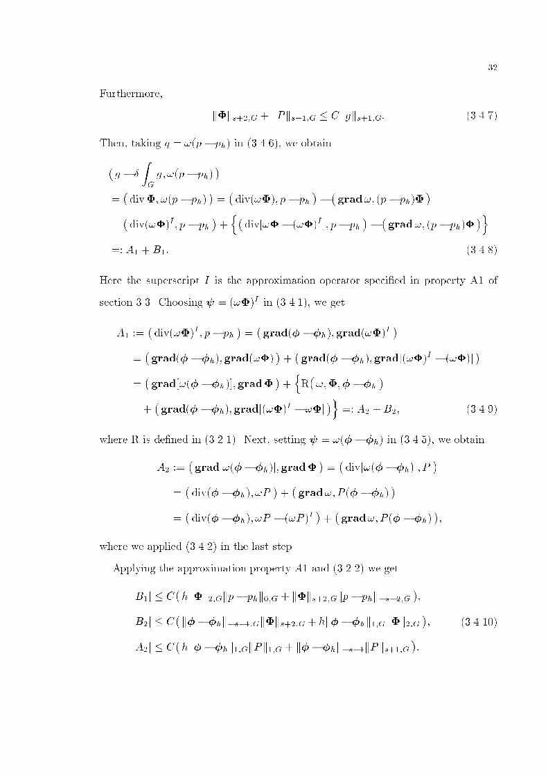
Furthermore�
k�ks���G � kPks���G � Ckgks���G� ������
Then� taking q � �p � ph� in ������� we obtain
�g �
ZG
g� �p� ph��
��div�� �p � ph�
���div���� p � ph
���grad�� p � ph��
���div���I � p � ph
��n�
div���� ���I �� p� ph���grad�� p � ph��
�o�� A� �B�� ������
Here the superscript I is the approximation operator speci�ed in property A� of
section ���� Choosing � � ���I in ������� we get
A� ���div���I � p� ph
���grad� ��h��grad���I
���grad� � �h��grad���
���grad� � �h��grad����I � ����
���grad��� ��h���grad�
��nR������ ��h
���grad� � �h��grad����I � ���
�o�� A� �B�� ������
where R is de�ned in ������� Next� setting � � �� � �h� in ������� we obtain
A� ���grad���� �h���grad�
���div���� �h��� P
���div�� �h�� �P
���grad��P � � �h�
���div�� �h�� �P � �P �I
���grad��P � � �h�
��
where we applied ������ in the last step�
Applying the approximation property A� and ������ we get
jB�j � C�hk�k��Gkp� phk��G � k�ks���Gkp� phk�s���G
��
jB�j � C�k�� �hk�s���Gk�ks���G � hk�� �hk��Gk�k��G
��
jA�j � C�hk�� �hk��GkPk��G � k�� �hk�s��kPks���G
��
������
��
Substituting ������ into ������ and combining the result with ������� ������� and
������� we arrive at ������� �
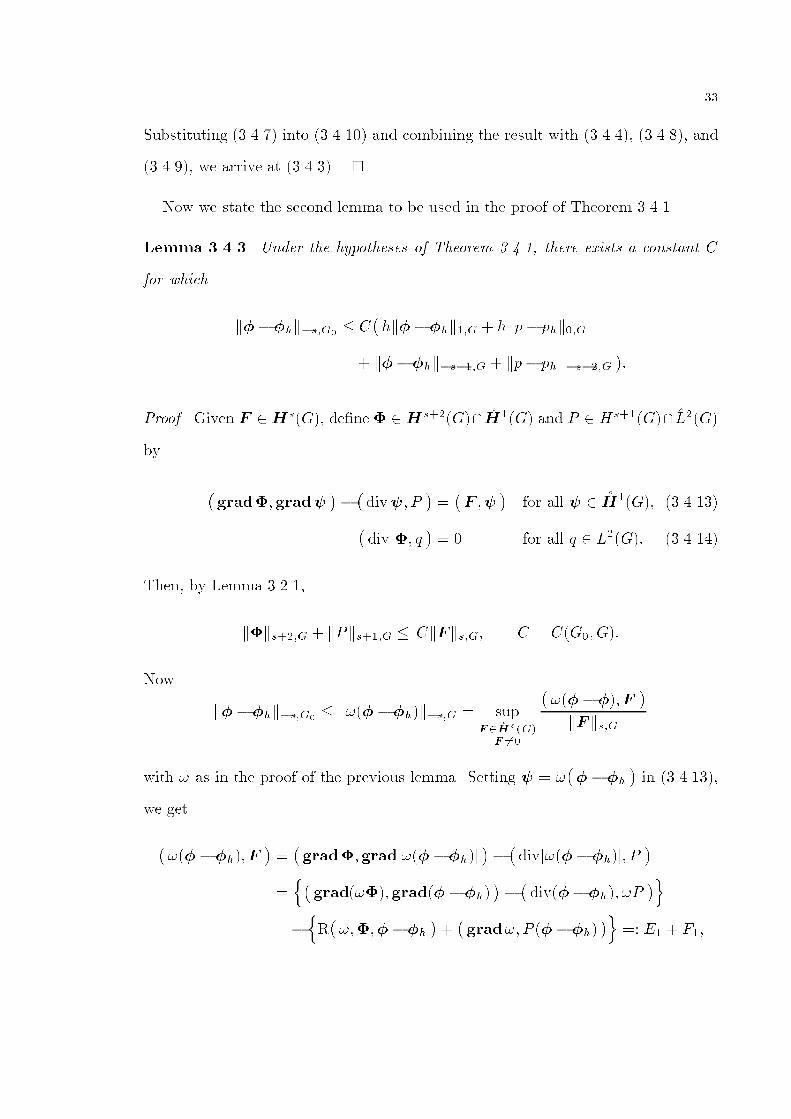
Now we state the second lemma to be used in the proof of Theorem ������
Lemma ������ Under the hypotheses of Theorem ������ there exists a constant C
for which
k�� �hk�s�G�� C
�hk�� �hk��G � hkp� phk��G
� k�� �hk�s���G � kp� phk�s���G��
Proof� Given F �HsG�� de�ne � �Hs��G�� H�G� and P � Hs��G�� #L�G�
by
�grad��grad�
���div�� P
���F ��
�for all � � H�G�� ��������
div �� q�� for all q � L�G�� �������
Then� by Lemma ������
k�ks���G � kPks���G � CkF ks�G� C � CG�� G��
Now
k� � �hk�s�G�� k�� � �h�k�s�G � sup
F��Hs�G�F ��
���� ���F
�kF ks�G
with � as in the proof of the previous lemma� Setting � � ��� � �h
�in ��������
we get
��� � �h��F
���grad��grad��� ��h��
���div���� �h��� P
��n�grad����grad� � �h�
���div�� �h�� �P
�o�nR������ ��h
���grad��P � � �h�
�o�� E� � F��

��
To estimate E�� we set q � �P �I in ������ and obtain
E� ��grad���I �grad� � �h�
��n�
div� � �h�� �P � �P �I�
��grad���� ���I ��grad� � �h�
�o�� E� � F��
Taking � � ���I in ������� we arrive at
E� ��grad���I �grad� ��h�
���div���I � p� ph
���div���� p � ph
���div����I � ����� p � ph
���grad�� p � ph��
���div����I � ����� p � ph
��
where we applied ������� in the last step� Applying ������ and the approximation
property A�� we have
j F� j� Ck���hk�s���Gk�ks���G � k�� �hk�s���GkPks���G��
j F� j � Chk�� �hk��GkPk��G � k�� �hk��Gk�k��G��
j E� j � C�kp� phk�s���Gk�ks���G � h kp� phk��Gk�k��G
��
From these bounds we get the desired result� �
Proof of Theorem ������ Let G� b G� b � � � Gs � G be concentric disks� First
applying Lemma ����� and Lemma ����� with s replaced by and G replaced by
G�� we obtain
k� ��hk��G�� kp� phk���G�
� C�hk�� �hk��G�
� hkp� phk��G�
� k� � �hk���G�� kp� phk���G�
��
To estimate k� � �hk���G�and kp � phk���G�
� we again apply Lemma ����� and
Lemma ������ this time with G� and G being replaced by G� and G� and s replaced
��
by �� Thus� we get
k� ��hk��G�� kp� phk���G�
� C�hk�� �hk��G�
� hkp� phk��G�
� k� � �hk���G�� kp� phk���G�
��
Continuing in this fashion� we obtain ������� �
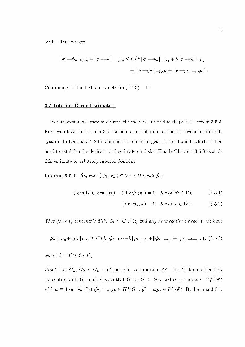
��� Interior Error Estimates
In this section we state and prove the main result of this chapter� Theorem ������
First we obtain in Lemma ����� a bound on solutions of the homogeneous discrete
system� In Lemma ����� this bound is iterated to get a better bound� which is then
used to establish the desired local estimate on disks� Finally Theorem ����� extends
this estimate to arbitrary interior domains�
Lemma ������ Suppose��h� ph
�� V h Wh satis�es
�grad�h�grad�
���div�� ph
�� for all � � V h� �������
div�h� q�� for all q � Wh� ������
Then for any concentric disks G� b G b �� and any nonnegative integer t� we have
k�hk��G��kphk��G�
� C�hk�hk��G�hkphk��G�k�hk�t�G�kphk�t���G
�� ������
where C � Ct�G�� G��
Proof� Let Gh� G� b Gh b G� be as in Assumption A�� Let G� be another disk
concentric with G� and G� such that G� b G� b Gh� and construct � � C�� G��
with � � on G�� Set f�h � ��h � H�G��� fph � �ph � L�G��� By Lemma ������
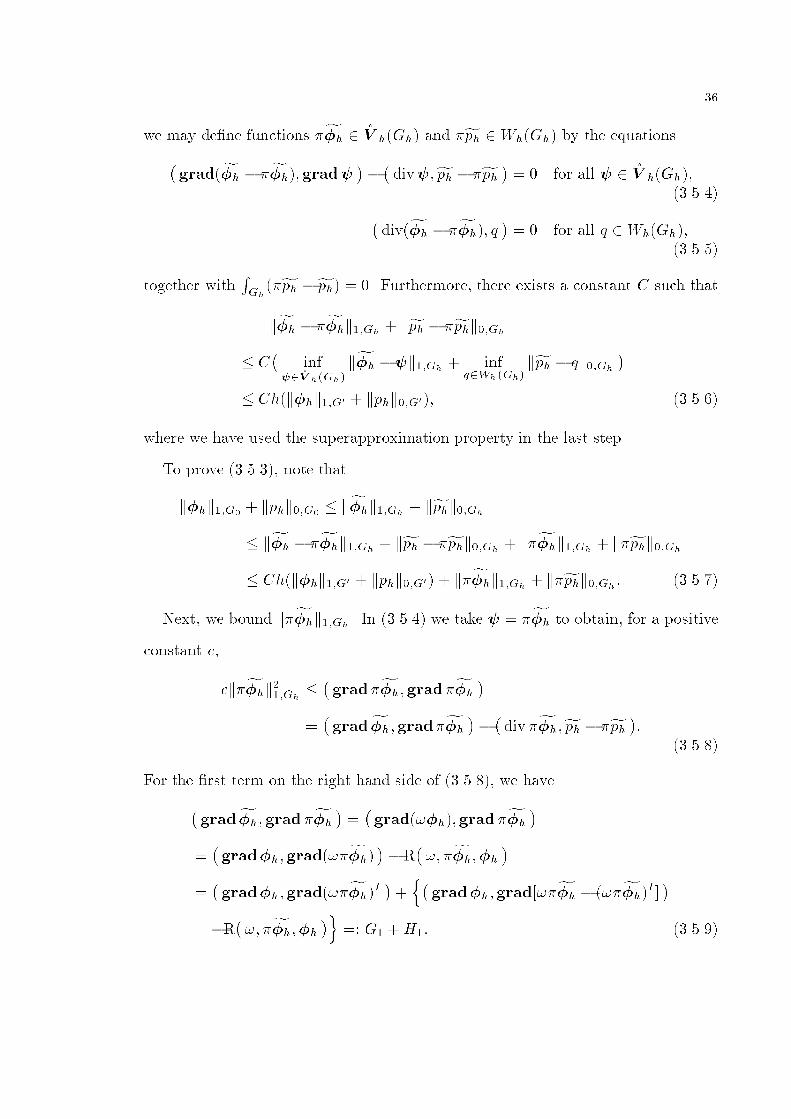
��
we may de�ne functions f�h � V hGh� and fph �WhGh� by the equations�gradf�h � f�h��grad� �� � div��fph � fph � � for all � � V hGh��
�������divf�h � f�h�� q � � for all q � WhGh��
������
together withRGh
fph �fph� � � Furthermore� there exists a constant C such that
kf�h � f�hk��Gh � kfph � fphk��Gh
� C�
inf���V h�Gh�
kf�h ��k��Gh � infq�Wh�Gh�
kfph � qk��Gh
�� Chk�hk��G� � kphk��G��� ������
where we have used the superapproximation property in the last step�
To prove ������� note that
k�hk��G�� kphk��G�
� kf�hk��Gh � kfphk��Gh
� kf�h � f�hk��Gh � kfph � fphk��Gh � kf�hk��Gh � kfphk��Gh
� Chk�hk��G� � kphk��G�� � kf�hk��Gh � kfphk��Gh� ������
Next� we bound kf�hk��Gh� In ������ we take � � f�h to obtain� for a positive
constant c�
ckf�hk���Gh��gradf�h�gradf�h �
��gradf�h�gradf�h �� �div f�h�fph � fph ��
������
For the �rst term on the right hand side of ������� we have�gradf�h�gradf�h � � �
grad��h��gradf�h ���grad�h�grad�f�h� � �R
��� f�h��h �
��grad�h�grad�f�h�I �� n�
grad�h�grad��f�h � �f�h�I � ��R
��� f�h��h �o �� G� �H�� ������
��
To bound G�� we take � � �f�h�I in ������ and get
G� ��div�f�h�I � ph �
��div�f�h�� ph �� �
div��f�h�I � �f�h�� ph ���div f�h� �ph �� �
grad�� phf�h �� �div��f�h�I � �f�h�� ph �
��div f�h�fph �� �
grad�� phf�h �� �div��f�h�I � �f�h�� ph �
���div f�h�fph ��H�� ������
Combining ������� ������� ������� and ������� we obtain
ckf�hk���Gh��div f�h�fph ��H� �H� �
�div f�h�fph � fph �
��div f�h� fph ��H� �H�� �������
Taking q � fph in ������� we get�div f�h� fph � � �
divf�h� fph � � �div��h�� fph �
��div�h� �fph �� �
grad�� fph�h ���div�h� �fph � �fph�I �� �
grad�� fph�h � �� H���������
where we used ������ at the last step� Applying the Schwartz inequality� �������
and the superapproximation property A�� we get
j H� j� C�h k�hk��G� � k�hk��G�
�kf�hk��Gh�
j H� j� C�kphk���G� � h kphk��G�
�kf�hk��Gh�
j H� j� C�h k�hk��G� � k�hk��G�
�kfphk��Gh �
Combining the above three inequalities with ������� and �������� and using the
arithmetic�geometry mean inequality� we arrive at
kf�hk���Gh� C�
�h�k�hk
���G� � k�hk
���G� � h�kphk
���G� � kphk
����G�
�� C�
�k�hk��G� � h k�hk��G�
�kfphk��Gh� �������
��
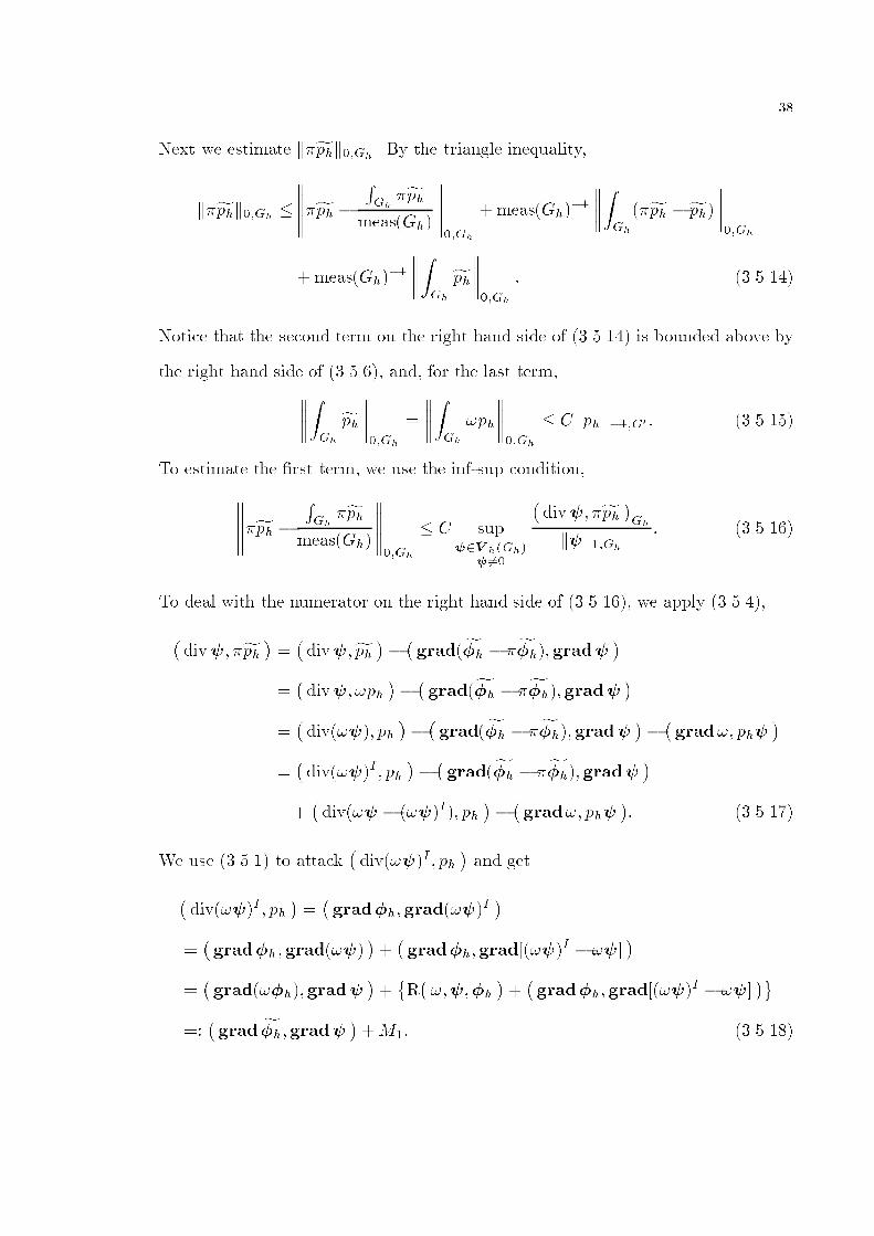
Next we estimate kfphk��Gh� By the triangle inequality�
kfphk��Gh �
�����fph �RGh
fphmeasGh�
�������Gh
�measGh���
����ZGh
fph �fph�������Gh
�measGh���
����ZGh
fph������Gh
� �������
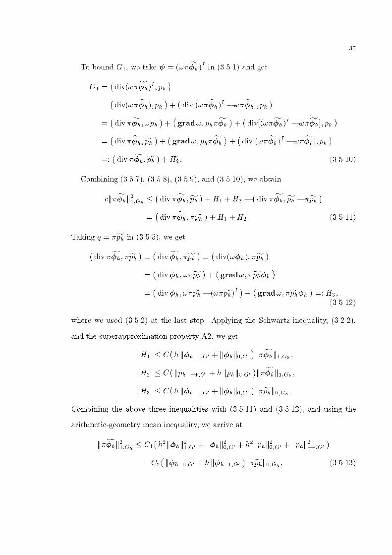
Notice that the second term on the right hand side of ������� is bounded above by
the right hand side of ������� and� for the last term�����ZGh
fph������Gh
�
����ZGh
�ph
������Gh
� Ckphk���G� � �������
To estimate the �rst term� we use the inf�sup condition������fph �RGh
fphmeasGh�
�������Gh
� C sup���V h�Gh�
� ��
�div�� fph �Gh
k�k��Gh
� �������
To deal with the numerator on the right hand side of �������� we apply �������
�div�� fph � � �
div��fph �� �gradf�h � f�h��grad� �
��div�� �ph
���gradf�h � f�h��grad� �
��div���� ph
���gradf�h � f�h��grad� �� �
grad�� ph��
��div���I � ph
���gradf�h � f�h��grad� �
��div�� � ���I�� ph
���grad�� ph�
�� �������
We use ������ to attack�div���I � ph
�and get
�div���I � ph
���grad�h�grad���
I�
��grad�h�grad���
���grad�h�grad����
I � ����
��grad��h��grad�
���R������h
���grad�h�grad����
I � ����
���gradf�h�grad� ��M�� �������
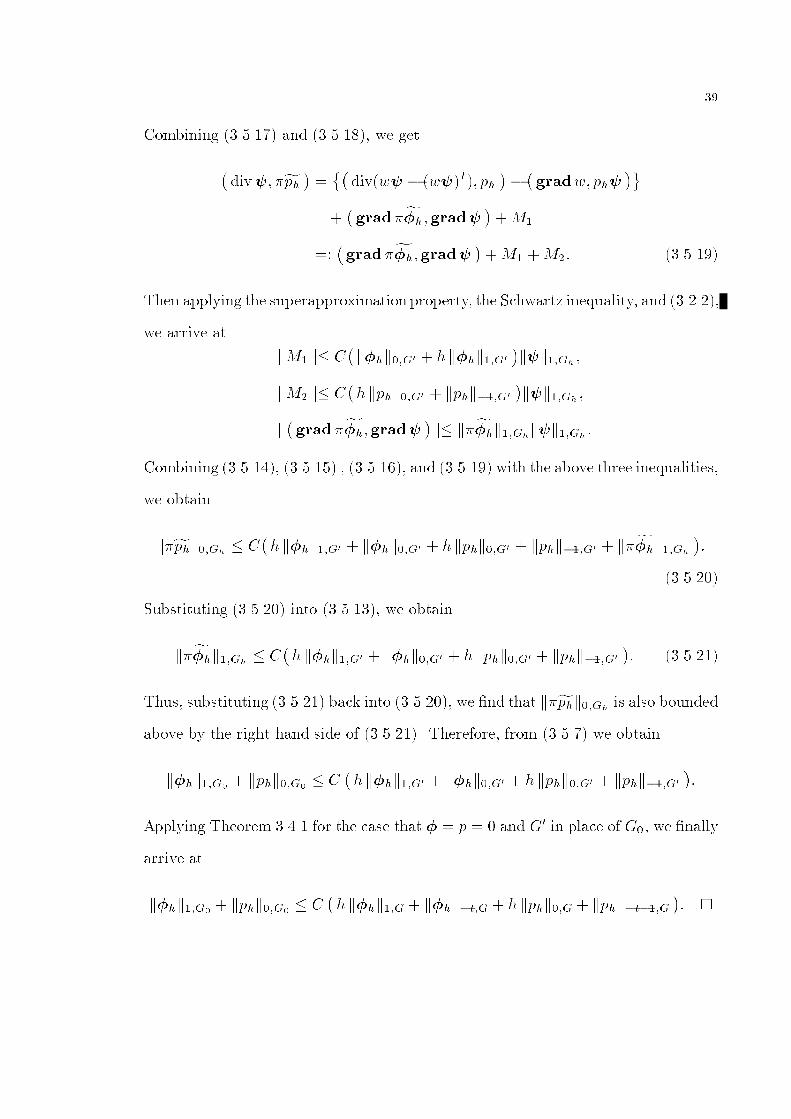
��
Combining ������� and �������� we get
�div�� fph � � ��
divw� � w��I�� ph���gradw� ph�
� ��gradf�h�grad� ��M�
���gradf�h�grad� ��M� �M�� �������
Then applying the superapproximation property� the Schwartz inequality� and �������
we arrive at
jM� j� C�k�hk��G� � h k�hk��G�
�k�k��Gh�
jM� j� C�h kphk��G� � kphk���G�
�k�k��Gh�
j�gradf�h�grad� � j� kf�hk��Ghk�k��Gh�
Combining �������� ������� � �������� and ������� with the above three inequalities�
we obtain
kfphk��Gh � C�h k�hk��G� � k�hk��G� � h kphk��G� � kphk���G� � kf�hk��Gh
��
������
Substituting ������ into �������� we obtain
kf�hk��Gh � C�h k�hk��G� � k�hk��G� � h kphk��G� � kphk���G�
�� �������
Thus� substituting ������� back into ������� we �nd that kfphk��Gh is also bounded
above by the right hand side of �������� Therefore� from ������ we obtain
k�hk��G�� kphk��G�
� C�h k�hk��G� � k�hk��G� � h kphk��G� � kphk���G�
��
Applying Theorem ����� for the case that � � p � and G� in place of G�� we �nally
arrive at
k�hk��G�� kphk��G�
� C�h k�hk��G � k�hk�t�G � h kphk��G � kphk�t���G
�� �
�
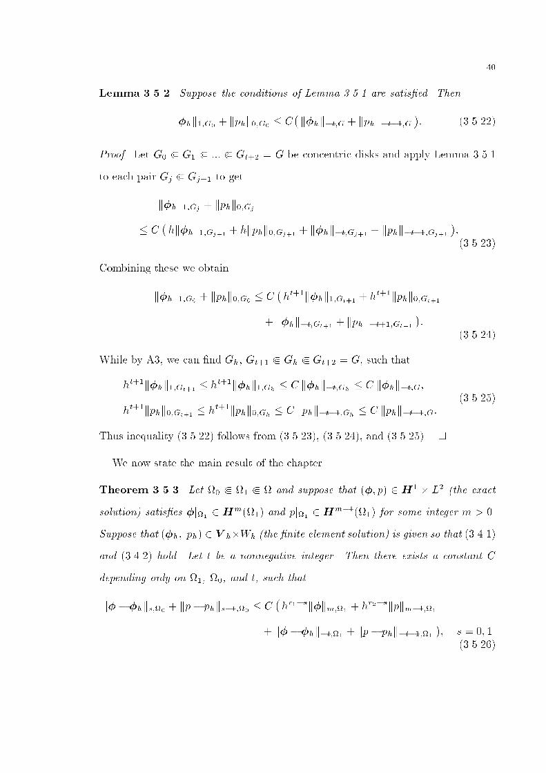
Lemma ������ Suppose the conditions of Lemma ����� are satis�ed� Then
k�hk��G�� kphk��G�
� C�k�hk�t�G � kphk�t���G
�� �������
Proof� Let G� b G� b ��� b Gt�� � G be concentric disks and apply Lemma �����
to each pair Gj b Gj�� to get
k�hk��Gj � kphk��Gj
� C�hk�hk��Gj�� � hkphk��Gj�� � k�hk�t�Gj�� � kphk�t���Gj��
���������
Combining these we obtain
k�hk��G�� kphk��G�
� C�ht��k�hk��Gt�� � ht��kphk��Gt��
� k�hk�t�Gt�� � kphk�t���Gt��
��
�������
While by A�� we can �nd Gh� Gt�� b Gh b Gt�� � G� such that
ht��k�hk��Gt�� � ht��k�hk��Gh � C k�hk�t�Gh � C k�hk�t�G�
ht��kphk��Gt�� � ht��kphk��Gh � C kphk�t���Gh � C kphk�t���G��������
Thus inequality ������� follows from �������� �������� and �������� �
We now state the main result of the chapter�
Theorem ������ Let �� b �� b � and suppose that �� p� � H� L� the exact
solution satis�es �j�� � Hm��� and pj�� � H
m����� for some integer m � �
Suppose that �h� ph� � V hWh the �nite element solution is given so that ������
and ������ hold� Let t be a nonnegative integer� Then there exists a constant C
depending only on ��� ��� and t� such that
k�� �hks��� � kp� phks����� � C�hr��sk�km��� � hr��skpkm�����
� k�� �hk�t��� � kp� phk�t������� s � � �
�������

��
with r� � mink� � ��m�� r� � mink� � ��m�� and k�� k� as in A��
The theorem will follow easily from a slightly more localized version�
Theorem ������ Suppose the hypotheses of Theorem ����� are ful�lled and� in
addition� that �� � G� and �� � G� are concentric disks� Then the conclusion of
the theorem holds�
Proof� Let G�� b G� be further concentric disks strictly contained between G� and
G and let Gh be a domain strictly contained between G� and G for which properties
A� and A� hold� Thus
G� b G�� b G� b Gh b G b ��
Take � � C�� G�� identically � on G�� and set e� � ��� ep � �p� Let e� � V hG��
ep �WhG� be de�ned by
�grad e� � e���grad� ���div�� ep� ep � � for all � � V hGh��
��������div e� � e��� q � � for all q �WhGh��
�������
together withRGh
ep �RGh
ep� Then using Lemma ����� and A� we have
k e�� e�k��Gh � kep� epk��Gh
� C�
inf���V h�Gh�
k e� ��k��Gh � infq�Wh�Gh�
kep � qk��Gh
�� C
�hr���k�km�Gh � hr���kpkm���Gh
�� �������
Let us now estimate k���hk��G�and kp�phk��G�
� First� the triangle inequality

��
gives us
k�� �hk��G�� kp� phk��G�
� k� � e�k��G�� kp� epk��G�
� k e� ��hk��G�� kep� phk��G�
� k e� � e�k��Gh � kep� epk��Gh � k e� � �hk��G�� kep � phk��G�
� C�hr���k�km�Gh � hr���kpkm���Gh
�� k e� ��hk��G�
� kep� phk��G��
������
From �������� ������� and ������� ������ we �nd
�grad�h � e���grad� �� �div�� ph � ep � � for all � � V hG
�����
div�h � e��� q � � for all q � WhG����
We next apply Lemma ����� to �h � e� and ph � ep with G replaced by G��� Then
it follows from ������� that
k�h � e�k��G�� kph � epk��G�
� C�k�h � e�k�t�G�� � kph � epk�t���G�� �
� C�k� � �hk�t�G�� � kp� phk�t���G�� � k� � e�k�t�G�� � kp� epk�t���G�� �
� C�k�� �hk�t�G � kp� phk�t���G � ke�� e�k��Gh � kep� epk��Gh
��
In the light of ������� �������� and the above inequality� we have
k� � �hk��G�� kp� phk��G�
��hr���k�km�G � hr���kpkm���G
� k� ��hk�t�G � kp� phk�t���G� ��������
Thus� we have proved the desired result for s � �� For s � � we just apply
Theorem ����� to the disks G� and G� and get
k� ��hk��G�� kp� phk���G�
� C hk�� �hk��G� � hkp� phk��G�
� k� � �hk�t�G� � kp� phk�t���G�� �

��
Then� applying ������� with G� replaced by G�� we obtain the desired result
k�� �hk��G�� kp� phk���G�
� C�hr�k�km�G � hr�kpkm���G
� k�� �hk�t�G � kp� phk�t���G�� �
Proof of Theorem ������ The argument here is same as in Theorem ��� of ����� Let
d � d��� where d� � dist ���� ����� Cover ��� with a �nite number of disks G�xi��
i � �� �� � � � �m centered at xi � ��� with diamG�xi� � d� Let Gxi�� i � �� �� � � � � k
be corresponding concentric disks with diamGxi� � �d� Applying Theorem ������
we have
k� ��hks�G��xi� � kp� phks���G��xi� � Ci
�hr��sk�km�G�xi� � hr��skpkm���G�xi�
� k�� �hk�t�G�xi� � kp� phk�t���G�xi���
�������
Then the inequality ������� follows by summing ������� for every i� �
�� An Example Application
As an example� we apply our general result to the Stokes system when the domain
is a non�convex polygon� in which case the �nite element approximation does not
achieve the optimal convergence rate in the energy norm on the whole domain� due
to the boundary singularity of the exact solution�
Assume that � is a non�convex polygon� Then it is known that the solution of
the Stokes system satis�es
� �Hs�� �H�� � p � Hs�
� �H����� p � H����� if �� b ��
for s � s�� where s� is a constant which is determined by the largest interior angle
of � cf� ������ For a non�convex polygonal domain we have ��� � s� � �� The

��
value of s� for various angles have been tabulated in ����� For example� for an
L�shaped domain� s� � �����
The MINI element was introduced by Arnold� Brezzi and Fortin in ��� as a stable
Stokes element with few degrees of freedom� Here the velocity is approximated
by the space of continuous piecewise linear functions and bubble functions and the
pressure is approximated by the space of continuous piecewise linear functions only�
Globally we have
k�� �hk� � kp� phk� � Chs�k�ks�� � kpks
��
which re$ects a loss of accuracy due to the singularity of the solutions�
In order to apply Theorem ������ we note that a standard duality argument as in
��� gives us
k�� �hk� � kp� phk�� � Ch�skF k��
Hence� according to Theorem ������ for �� b �� b �� we have
k�� �hk���� � kp� phk���� � C�hk�k���� � hkpk���� � h�s kF k�
��
Since �s � �� the �nite element approximation achieves the optimal order of conver�
gence rate in the energy norm in interior subdomains�
��
CHAPTER �
INTERIOR ESTIMATES FOR
A FINITE ELEMENT METHOD FOR
THE REISSNERMINDLIN PLATE MODEL
��� Introduction
The Reissner�Mindlin plate model describes deformation of a plate with small to
moderate thickness subject to a transverse load� The �nite element method for this
model was studied extensively cf� ����� ���� and references therein� and it has been
known for a long time that a direct application of standard �nite element methods
usually leads to unreasonly small solution� as the plate thickness approaches zero�
This is usually called the !locking" phenomenon of the �nite element method for the
Reissner�Mindlin plate ����� ����
The reason behind the locking phenomenon is well known� as the plate thickness
becomes very small� the numerical scheme tries to enforce a discrete version of
the Kircho� constraint on the displacement and the rotation �ber normal to the
midplane� If the �nite element spaces for those two quantities are not chosen wisely�
then� together with boundary conditions� the numerical solution reduces to the trivial
solution�
Another di�culty relating to the Reissner�Mindlin plate model is that the solution
possesses boundary layers� having the plate thickness as the singular parameter� As
usual� the strength of the boundary layer is sensitive to the boundary condition� The
structure of the dependence of the solution on the plate thickness was analyzed in
detail by Arnold and Falk ���� ����

��
The purpose of this chapter is to obtain the interior error estimate for the Arnold�
Falk element ��� for the Reissner�Mindlin plate model� This element is the �rst to
achieve a locking�free �rst order optimal� convergence for the Reissner�Mindlin plate
under the hard clamped boundary condition�� However� it does not retain the same
order of convergence rate for the plate under the soft simply supported boundary
condition� due to a stronger boundary layer e�ect� By applying the interior estimate
to the soft simply supported plate� we are able to obtain the interior convergence
rate of the Arnold�Falk element and show that it still possesses almost� �rst order
convergence rate in the region away from the boundary�
The construction of the Arnold�Falk element is based on an equivalence between
the plate equations and an uncoupled system of two Poisson equations plus a Stokes�
like system ���� Arnold and Falk used the nonconforming linear element for the
Poisson equation and the MINI element for the Stokes�like system� So the global
or interior� analysis of the Arnold�Falk element consists of two parts� one for the
nonconforming method for the Poisson equation and another for the MINI element
for the Stokes�like system� Recall that in Chapter � we obtained interior estimates for
the nonconforming element for the Poisson equation� So the task here is essentially
to analyze the interior error estimate of the MINI element for the Stokes�like system�
The organization of chapter is as follows� Section ��� presents the Reissner�
Mindlin plate equations and its reformulation under the Helmholtz decomposition
for the shear stress� The interior regularity of the solution of the singularly per�
turbed system is studied in section ���� The Arnold�Falk element is introduced in
section ���� Section ��� is devoted to the interior duality analysis of the variant of
the Stokes system� In section ��� we �rst obtain the interior estimate of the MINI
element Theorem ������ for the Stokes�like system with perturbation and then use
it to get the interior estimate of the Arnold�Falk element for the Reissner�Mindlin

��
plate model Theorem ������� which is the main result of the chapter� As an appli�
cation of the general theory we develop� we consider the soft simply supported plate
in section ���� We will show that globally� the Arnold�Falk element only achieves
almost� h��� order convergence for the rotation Theorem ������� but away from
the boundary layer� almost� optimal order convergence rate can be obtained The�
orem ������� Finally� numerical results are shown in section ��� which con�rm the
theoretical predictions�
��� Notations and the Reissner�Mindlin Plate Model
The following operators are standard�
div
�t�� t��t�� t��
��
��t����x � �t����y
�t����x � �t����y
��
curl p �
���p��y
�p��x
�� rot� � �����y � �����x�
Let � denote the region in R� occupied by the midsection of the plate� and
denote by w and � the transverse displacement of � and the rotation of the �bers
normal to �� respectively� Under the soft simply supported boundary condition�
the Reissner�Mindlin plate model determines w��� as the unique solution to the
following variational problem�
Find w��� � H� H� such that
a������t����gradw���grad� � g� � for all ��� � H�H�� ������
Here g is the scaled transverse loading function� t the plate thickness�
� � E���� � �� with E the Young�s modulus� � the Poisson ratio� and � the

��
shear correction factor� The bilinear form a is
a���� �E
���� ���
Z�
�����x
� �����y
�����x
�
������x
�����y
�����y
��� �
�
�����y
�����x
������y
�����x
�
�
Z�
CE�� � E���
Here� E�� is the symmetric part of the gradient of � and C is a fourth order tensor
de�ned by the bilinear form a�
Following Brezzi and Fortin ����� equation ������ can be reformulated by using
the Helmholtz Theorem to decompose the shear strain vector
�t��gradw � �� � grad r � curl p� ������
with r� p� � H� #H��
Equation ������ now becomes
Find r��� p� w� � H� H� #H� H� such that
grad r�grad� � g� � for all � H�� �������CE��� E ��
���curl p��
���grad r��
�for all � �H�� ������
��� curl q� � ���t�curl p� curl q� � for all q � #H�� ������
gradw�grad s� � � � ���t� grad r�grad s� for all s � H�� ������
Obviously the function r in ������ is independent of t and the functions �� p� and
w are not� It has been shown in ��� that the transverse displacement w does not
su�er from the boundary layer e�ect under all boundary conditions� However� the
regularity of solution �� p� for system ������ and ������ depends on the boundary
condition imposed on the plate� For example� under the hard clamped boundary

��
condition then� � is to be found in space H�� rather than H��� the following holds
���
k�k� � kpk� � Ckgk��
with the constant C independent of the plate thickness t� This guarantees the MINI
element to achieve a locking free �rst order convergence rate for the system ������
and ������ ����
But the above estimate does not hold for the soft simply supported plate� In this
case� one can only expect that the H��� norm of function � and the H��� norm of
function p to be bounded above� independent of the small parameter t ���� This is
obviously not enough for the �nite element method to achieve �rst order convergence
rate� It is also easy to see that a complete understanding of the dependence of the
regularity of the solution on the small parameter t is of crucial importance for the
convergence analysis of the �nite element method� However� for the purpose of
interior estimates� we need only know the inteiror regularity of the solution of the
Stokes�like system� This will be given in the next section�
In the following� we introduce some notations that will be used in the interior
estimate�
Let G be an open subset of �� � � C�� G�� and s an integer� For � � HsG��
� �H�s��G�� P � HsG�� and Q � H�s��G�� de�ne
R������ ��CE���� E ��
���CE��� E���
�and
R����P�Q
���curl�P �� curlQ
���curlP� curl�Q�
��
Then
jR������
�� Ck�kt�Gk�k�t���G ������
�
and
jR����P�Q
�� CkPkt�GkQk�t���G� ������
for non�negative integers t � s�
��� An Interior Regularity Result
In this section we present an interior regularity result for the solution of the
singularly perturbed Stokes�like system under the homogeneous Dirichlet boundary
condition� We will show that the regularity of the solution in the interior region
is not a�ected by the boundary layer� This will be used in section ��� for the the
interior duality analysis of the MINI element�
The proof basically follows that in ��� Theorem ���� for proving the regularity of
the solution of the hard�clamped plate and uses the standard approach for analyzing
interior regularities for solutions of elliptic equations�
Theorem ������ Let F �HsG� and K � Hs��G� � #L�G�� where integer s �
and G is a disk� Then there exists a unique solution �� P � �Hs��G�� H�G�
Hs��G� � #L�G� such that
CE��� E��� � curl P��� � ��F � for all � � H�G�� ������
��� curlQ� � ���t�curlQ� curl P � � Q�K� for all Q � H�G�� ������
Moreover�
k�k��G � kPk��G � tkPk��G � t�kPk��G � C�kF k��G � kKk��G
�� ������
k�ks���G�� kPks���G�
� tkPks���G�� t�kPks���G�
� C�kF ks�G � kKks���G
��
������
for an arbitrary disk G� b G�

��
Proof� The inequality
k�k��G � kPk��G � tkPk��G � C�kF k��G � kKk��G
�is proved in ��� for K � when a���� is simpli�ed into grad��grad��� i�e��
CE��� E��� is replaced by grad��grad�� in ������� By checking the proof
there and using the fact that bilinear form�CE��� E��
�is coercive on space H��
we can conclude that the same estimate still applies to the current case� What we
will do next is to follow the same proof to show that the estimate is still true for
K �� � At the same time� we will prove that t�kPk��G is also bounded above by the
right hand side of �������
De�ne ��� P �� � H�G� #L�G� as the solution of ������ and ������ with t
set equal to zero�
CE��� E���� � P �� rot�� � ��F � for all � � H�G��������
�rot��� Q� � Q�K� for all Q � L�G��������
This is a Stokes like system which admits a unique solution� Moreover� the standard
regularity theory gives ���
k��k��G � kP �k��G � C�kF k��G � kKk��G
�� ������
From ������� ������� ������� and ������� we get�CE� ����� E ��
���curlP � P ����
�� for all � � H�G���
����� curlQ�� ���t�
�curlP� curlQ
�� for all Q � H�G��
which imply�CE� ����� E��
���curlP � P ����
���� ���� curlQ
�� ���t�
�curlP � P ��� curlQ
�� ����t�
�curlP �� curlQ
�for all �� Q� � H�G� H�G��
��
Choosing � � ���� and Q � P � P �� we obtain
k����k���G � t�kP � P �k���G � Ct�kP �k��GkP � P �k��G�
It easily follows that
k����k��G � tkP � P �k��G � CtkP �k��G � CtkF k��G � kKk��G�� ������
Hence also
kPk��G � CkF k��G � kKk��G��
Applying standard estimates for second�order elliptic problems to ������� we further
obtain
k�k��G � CkPk��G � kF k��G� � CkF k��G � kKk��G�� ������
Now from ������ and the de�nition of �� i�e�� ������� we get
���t�curlP� curlQ� � ��� curlQ�� K�Q� � �� ��� curlQ�
for all Q � H�G��
Thus P is the weak solution of the boundary value problem
��P � �t�� rot�� ��� in G��P
�n� on �G�
and by standard a priori estimates
kPk��G � Ct��k����k��G � Ct��kF k��G � kKk��� ������
and
kPk��G � Ct��k����k��G � Ct��k�k��G�k��k��G� � Ct��kF k��G�kKk��G��
�������
��
where we apply ������ in deriving ������� and ������� ������ in deriving ��������
This completes the proof of �������
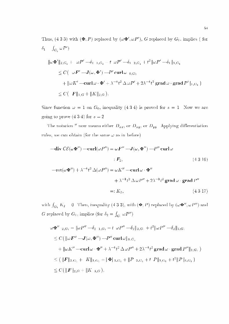
In order to prove ������� we take a disk G� such that G� b G� b G� Find a
cut�o� function � � C�� G�� with � � � on G�� We will use the notation � � Dx or
Dy� say for example� P � can be either Px or Py� Then� by di�erentiation rules� it is
easy to obtain
�div CE����� curl�P �� � �F � � J������ P � curl�
�� F�� �������
� rot���� � ���t���P �� � �K � � curl� ��� � ���t���P �
� ����t� grad� � gradP �
�� K�� �������
where
J����� �� div CE����� � div CE����
with
jJ�����j � Ck��k��G��
Obviously� ZG�
K� �
ZG�
�� rot���� � ���t���P ��
�� �
Z�G�
���� � s � ���t���P ����n
�� �
because both � and grad� vanish on �G�� Moreover� we see that ���� �P ��
satis�es
CE��� E������ curl�P ����� � ��F�� for all � � H�G����������
����� curlQ� � ���t�curlQ� curl�P ��� � Q�K�� for all Q � H�G����������
��
Thus� ������ with �� P � replaced by ���� �P ��� G replaced by G�� implies for
� �RG�
�P ��
k���k��G�� k�P � � �k��G�
� tk�P � � �k��G�� t�k�P � � �k��G�
� C�k�F � � J������ P � curl�k��G�
� k�K � � curl� ��� � ���t���P � � ����t� grad� � gradP �k��G�
�� C
�kF k��G � kKk��G
��
Since function � � � on G�� inequality ������ is proved for s � �� Now we are
going to prove ������ for s � ��
The notation �� now means either Dxx� or Dxy� or Dyy� Applying di�erentiation
rules� we can obtain for the same � as in before�
�div CE������ curl�P ��� � �F �� � J������� P �� curl�
�� F�� �������
� rot����� � ���t���P ��� � �K �� � curl� ����
� ���t���P �� � ����t� grad� � gradP ��
�� K�� �������
withRG�
K� � � Then� inequality ������� with �� P � replaced by ����� �P ��� and
G replaced by G�� implies for � �RG�
�P ���
k����k��G�� k�P �� � �k��G�
� tk�P �� � �k��G�� t�k�P �� � �k��G�
� C�k�F �� � J������� P �� curl�k��G�
� k�K �� � curl� ���� � ���t���P �� � ����t� grad� � gradP ��k��G�
���kF k��G�
� kKk��G�� k�k��G�
� kPk��G�� tkPk��G�
� t�kPk��G�
�� C
�kF k��G � kKk��G
��
��
where in the last step we use ������ with s � � and G� replaced by G�� Since � � �
on G�� so inequality ������ is proved for s � �� Same arguments� together with an
induction on s could be used to prove ������ for s � �� �
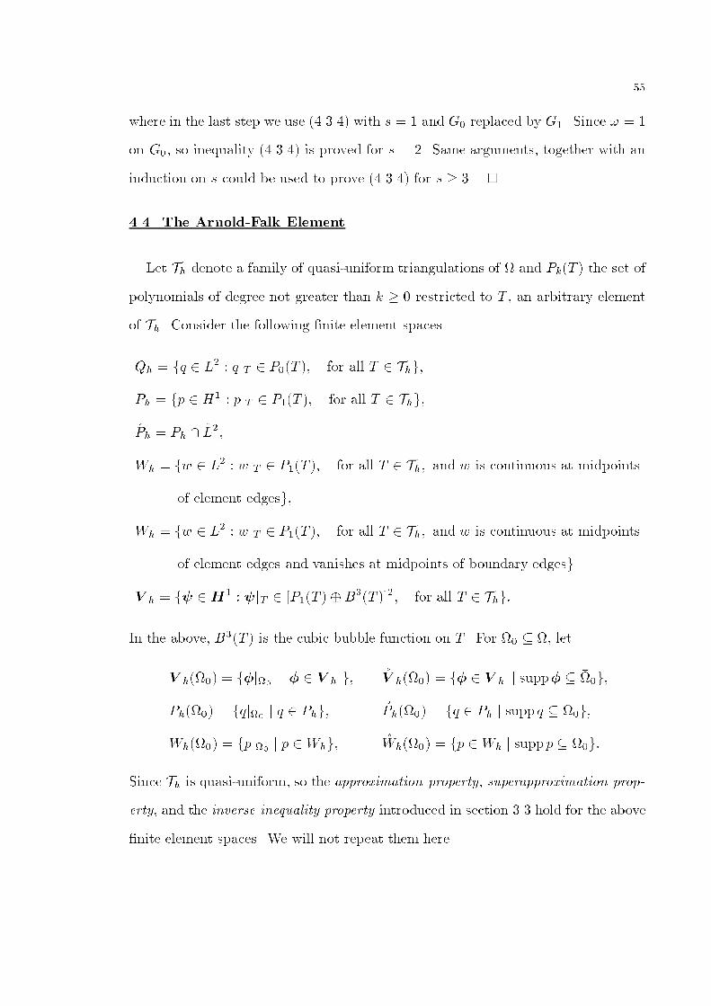
���� The ArnoldFalk Element
Let Th denote a family of quasi�uniform triangulations of � and PkT � the set of
polynomials of degree not greater than k � restricted to T � an arbitrary element
of Th� Consider the following �nite element spaces
Qh � fq � L� � qjT � P�T �� for all T � Thg�
Ph � fp � H� � pjT � P�T �� for all T � Thg�
#Ph � Ph � #L��
Wh � fw � L� � wjT � P�T �� for all T � Th� and w is continuous at midpoints
of element edgesg�
�Wh � fw � L� � wjT � P�T �� for all T � Th� and w is continuous at midpoints
of element edges and vanishes at midpoints of boundary edgesg
V h � f� �H� � �jT � �P�T � B�T ���� for all T � Thg�
In the above� B�T � is the cubic bubble function on T � For �� � �� let
V h��� � f�j�� j � � V h g� V h��� � f� � V h j supp� � ���g�
Ph��� � fqj�� j q � Phg� Ph��� � fq � Ph j suppq � ���g�
Wh��� � fpj�� j p �Whg� Wh��� � fp � Wh j suppp � ���g�
Since Th is quasi�uniform� so the approximation property� superapproximation prop�
erty� and the inverse inequality property introduced in section ��� hold for the above
�nite element spaces� We will not repeat them here�
��
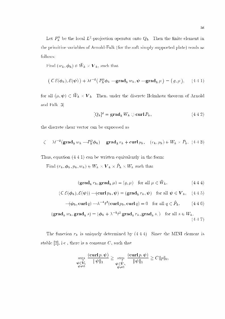
Let P �h be the local L��projection operator onto Qh� Then the �nite element in
the primitive variables of Arnold�Falk for the soft simply supported plate� reads as
follows�
Find wh��h� � �Wh V h� such that
�C E�h�� E��
�� �t��
�P �h�h � gradh wh�� � gradh
���g�
�� ������
for all ��� � �Wh V h� Then� under the discrete Helmhotz theorem of Arnold
and Falk ���
�Qh�� � gradh
�Wh curlPh� ������
the discrete shear vector can be expressed as
� � �t��gradh wh � P �h�h� � gradh rh � curl ph� rh� ph� � �Wh #Ph� ������
Thus� equation ������ can be written equivalently in the form�
Find rh��h� ph� wh� � �Wh V h #Ph �Wh such that
gradh rh�gradh � � g� � for all � �Wh� ������
C E�h�� E��� � curl ph��� � gradh rh��� for all � � V h� ������
��h� curl q� � ���t�curl ph� curl q� � for all q � #Ph� ������
gradh wh�gradh s� � �h � ���t� gradh rh�gradh s� � for all s � �Wh�������
The function rh is uniquely determined by ������� Since the MINI element is
stable ���� i�e�� there is a constant C� such that
sup��Vh� ��
curl p���
k�k�� sup���V h� ��
curl p���
k�k�� Ckpk��
��
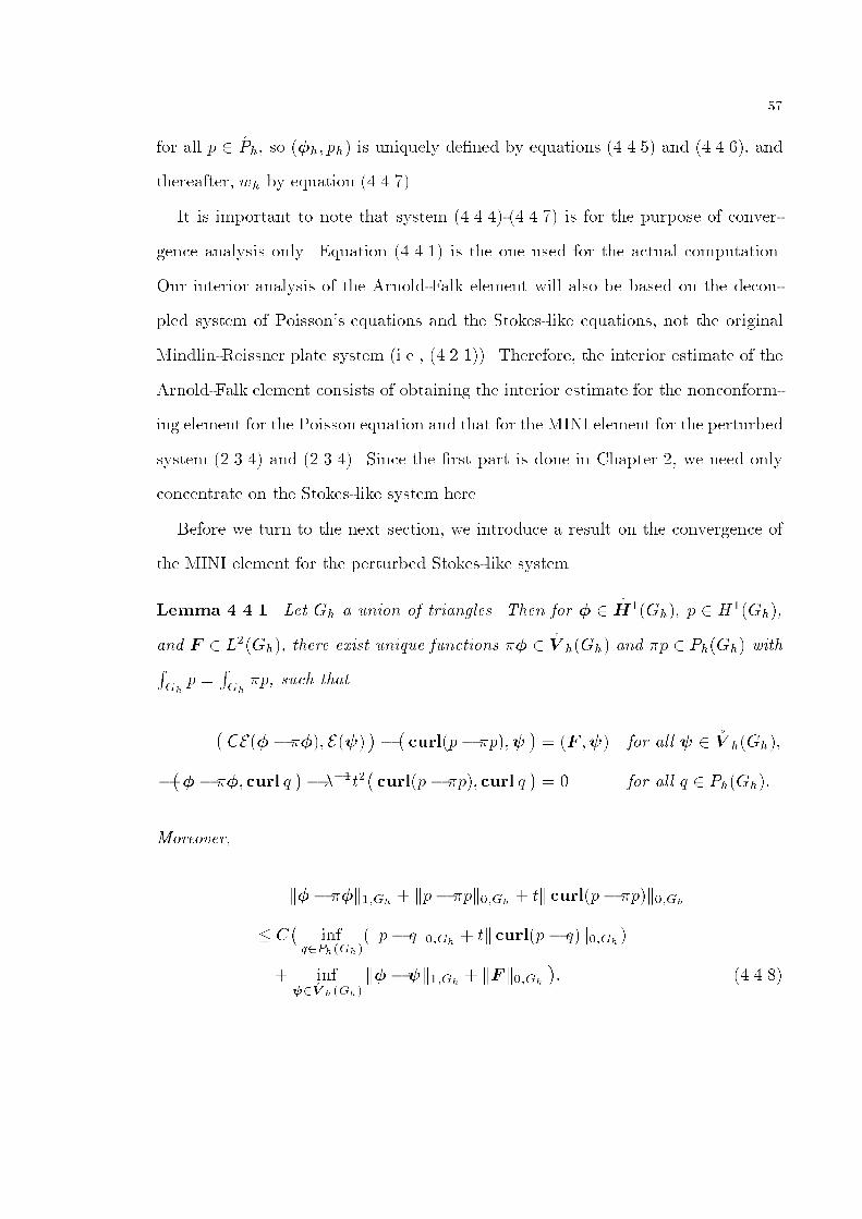
for all p � #Ph� so �h� ph� is uniquely de�ned by equations ������ and ������� and
thereafter� wh by equation �������
It is important to note that system ������������� is for the purpose of conver�
gence analysis only� Equation ������ is the one used for the actual computation�
Our interior analysis of the Arnold�Falk element will also be based on the decou�
pled system of Poisson�s equations and the Stokes�like equations� not the original
Mindlin�Reissner plate system i�e�� �������� Therefore� the interior estimate of the
Arnold�Falk element consists of obtaining the interior estimate for the nonconform�
ing element for the Poisson equation and that for the MINI element for the perturbed
system ������ and ������� Since the �rst part is done in Chapter �� we need only
concentrate on the Stokes�like system here�
Before we turn to the next section� we introduce a result on the convergence of
the MINI element for the perturbed Stokes�like system�
Lemma ������ Let Gh a union of triangles� Then for � � H�Gh�� p � H�Gh��
and F � L�Gh�� there exist unique functions � � V hGh� and p � PhGh� withRGh
p �RGh
p� such that
�CE� � ��� E ��
���curlp� p���
�� F ��� for all � � V hGh��
��� � �� curl q
�� ���t�
�curlp � p�� curl q
�� for all q � PhGh��
Moreover�
k�� �k��Gh � kp� pk��Gh � tk curlp� p�k��Gh
� C�
infq�Ph�Gh�
kp� qk��Gh � tk curlp � q�k��Gh�
� inf���V h�Gh�
k� ��k��Gh � kF k��Gh
�� ������
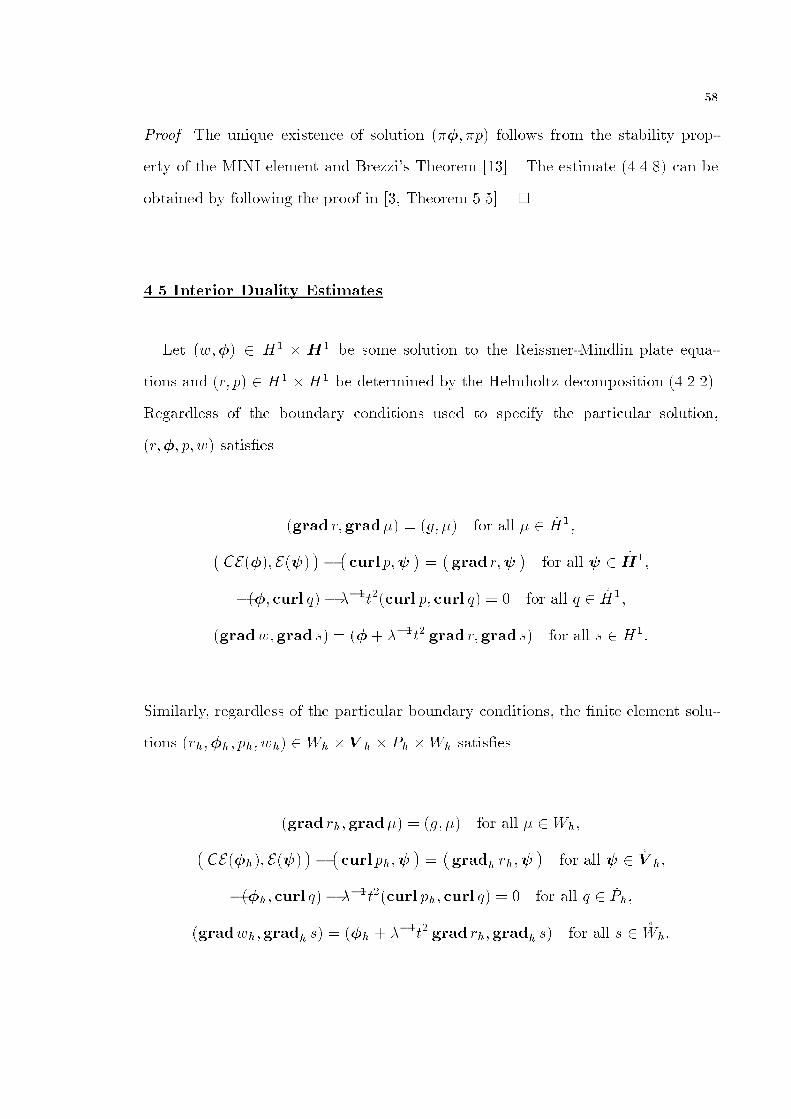
��
Proof� The unique existence of solution �� p� follows from the stability prop�
erty of the MINI element and Brezzi�s Theorem ���� � The estimate ������ can be
obtained by following the proof in ��� Theorem ����� �
��� Interior Duality Estimates
Let w��� � H� H� be some solution to the Reissner�Mindlin plate equa�
tions and r� p� � H� H� be determined by the Helmholtz decomposition �������
Regardless of the boundary conditions used to specify the particular solution�
r��� p� w� satis�es
grad r�grad� � g� � for all � H���CE��� E ��
���curl p��
���grad r��
�for all � � H��
��� curl q� � ���t�curl p� curl q� � for all q � H��
gradw�grad s� � � � ���t� grad r�grad s� for all s � H��
Similarly� regardless of the particular boundary conditions� the �nite element solu�
tions rh��h� ph� wh� �Wh V h Ph Wh satis�es
grad rh�grad� � g� � for all � Wh��CE�h�� E��
���curl ph��
���gradh rh��
�for all � � V h�
��h� curl q� � ���t�curl ph� curl q� � for all q � Ph�
gradwh�gradh s� � �h � ���t� grad rh�gradh s� for all s � Wh�
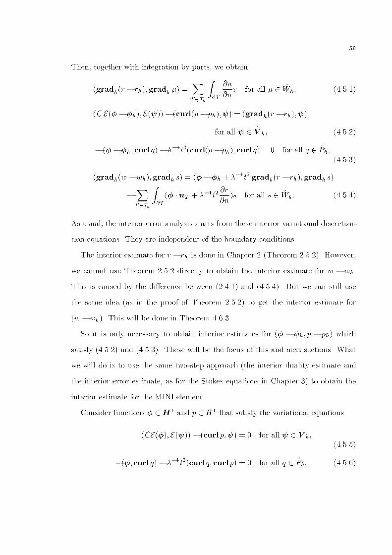
��
Then� together with integration by parts� we obtain
gradhr � rh��gradh � �XT�Th
Z�T
�u
�nv for all � Wh� ������
C E� � �h�� E ���� curlp � ph���� � gradhr � rh����
for all � � V h� ������
� � � �h� curl q� � ���t�curlp � ph�� curl q� � for all q � Ph�������
gradhw �wh��gradh s� � �� �h � ���t� gradhr � rh��gradh s�
�XT�Th
Z�T
� � nT � ���t��r
�n�s for all s � Wh� ������
As usual� the interior error analysis starts from these interior variational discretiza�
tion equations� They are independent of the boundary conditions�
The interior estimate for r � rh is done in Chapter � Theorem ������� However�
we cannot use Theorem ����� directly to obtain the interior estimate for w � wh�
This is caused by the di�erence between ������ and ������� But we can still use
the same idea as in the proof of Theorem ������ to get the interior estimate for
w � wh�� This will be done in Theorem ������
So it is only necessary to obtain interior estimates for � � �h� p � ph� which
satisfy ������ and ������� These will be the focus of this and next sections� What
we will do is to use the same two�step approach the interior duality estimate and
the interior error estimate� as for the Stokes equations in Chapter �� to obtain the
interior estimate for the MINI element�
Consider functions � �H� and p � H� that satisfy the variational equations
CE��� E ��� � curl p��� � for all � � V h�������
��� curl q� � ���t�curl q� curl p� � for all q � Ph� ������

�
We have the following result�
Theorem ������ Assume � � H� and p � H� satisfy ������ and ������� Let
G� b G b � be two concentric disks� Then for any integer � � � the following
holds
k�k��G��kpk���G�
� Chk�k��G�hkpk��G�htk curl pk��G�k�k���G�kpk�����G��
������
Proof� Find a diskG� such that G� b G� b G and construct a function � � C�� G��
with � � � on G�� Then� for any non�negative integer s�
k�k�s�G�� k��k�s�G � sup
F��Hs�G�F ��
���F �
kF ks�G� ������
To estimate the right hand side of ������� we de�ne �� P � through ������ and
������ with K � � Then take � � �� in ������ to obtain
����F
���CE���� E��
������ curlP
���CE��� E ���
����� curl�P �
��R������ �
�curl��P�
����CE��� E ���I
����� curl�P �
� ���CE��� E ���� ���I �
��R������ �
�curl��P�
� �� A� �B�� ������
Here the superscript I is the approximation operator� Chosing � to be ���I in

��
������ we get
A� ��curl p� ���I
����� curl�P �
���curl p� ��
����� curl�P �
���curl p� ���I � ��
����curl�p���
����� curl�P �
� ���curl�� p�
���curl p� ���I � ��
� �� A� �B�� ������
Taking Q � �p in ������ with K � �� we obtain
A� � ����t��curl�p�� curl P
����� curl�P �
�� ����t�
�curl p� curl�P �
����� curl�P �
�� ���t�R���P� p�
� �����t�
�curl p� curl�P �I
����� curl�P �
� �����t�
�curl p� curl��P �I � �P �
�� ���t�R���P� p�
�� A� �B��
�������
Substituting q � �P �I in ������� we have
A� ���� curl�P �I
����� curl�P �
����� curl��P �I � �P �
�� �������
Combining ������ through �������� we get
����F
�� B� �B� �B� �A�� �������
Then applying the approximation property� ������� ������� integration by parts� and
the Schwarz inequality� we obtain
j B� j� C�hk�k��G�
k�k��G�� k�k�s���G�
k�ks���G�� kPks���G�
���
j B� j� C�hkpk��G�
k�k��G�� kpk�s���G�
k�ks���G�
��
j B� j� C�ht�k curl pk��G�
kPk��G�� t�kpk�s���G�
kPks���G�
��
j A� j� Chk�k��G�kPk��G�
�
�������
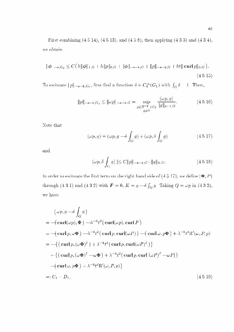
��
First combining �������� �������� and ������� then applying ������ and �������
we obtain
k�k�s�G�� C
�hk�k��G � hkpk��G � k�k�s���G � kpk�s���G � htk curl pk��G
��
�������
To estimate kpk�s���G�� �rst �nd a function � C�� G�� with
RG � �� Then�
kpk�s���G�� k�pk�s���G � sup
g��Hs���G�g ��
�p� g�
kgks���G� �������
Note that
�p� g� � �p� g �
ZG
g� � �p�
ZG
g� �������
and
j �p�
ZG
g� j� Ckpk�s���G � kgk��G� �������
In order to estimate the �rst term on the right hand side of �������� we de�ne �� P �
through ������ and ������ with F � � K � g � RGg� Taking Q � �p in �������
we have
��p� g �
ZG
g�
� ��curl�p���
�� ���t�
�curl�p�� curl P
�� �
�curl p� ��
�� ���t�
�curl p� curl�P �
���curl�� p�
�� ���t�R���P� p�
� ���curl p� ���I
�� ���t�
�curl p� curl�P �I
� ���curl p� ���I � ��
�� ���t�
�curl p� curl��P �I � �P �
���curl�� p�
�� ���t�R���P� p�
�� C� �D�� �������
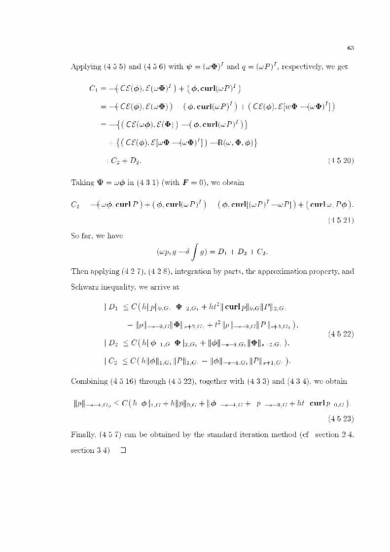
��
Applying ������ and ������ with � � ���I and q � �P �I � respectively� we get
C� � ��CE��� E ���I
����� curl�P �I
�� �
�CE��� E ���
����� curl�P �I
���CE��� E �w� � ���I �
�� �
��CE���� E ��
����� curl�P �I
� ���CE��� E ���� ���I �
��R������
�� C� �D�� ������
Taking � � �� in ������ with F � �� we obtain
C� � ����� curl P
����� curl�P �I
����� curl��P �I ��P �
���curl��P�
��
�������
So far� we have
�p� g �
Zg� � D� �D� �C��
Then applying ������� ������� integration by parts� the approximation property� and
Schwarz inequality� we arrive at
j D� j� C�hkpk��G�
k�k��G�� ht�k curl pk��GkPk��G�
� kpk�s���Gk�ks���G�� t�kpk�s���GkPks���G�
��
j D� j� C�hk�k��Gk�k��G�
� k�k�s���G�k�ks���G�
��
j C� j� C�hk�k��G�
kPk��G�� k�k�s���G�
kPks���G�
��
�������
Combining ������� through �������� together with ������ and ������� we obtain
kpk�s���G�� C
�hk�k��G � hkpk��G � k�k�s���G � kpk�s���G � htk curl pk��G
��
�������
Finally� ������ can be obtained by the standard iteration method cf� section ����
section ����� �
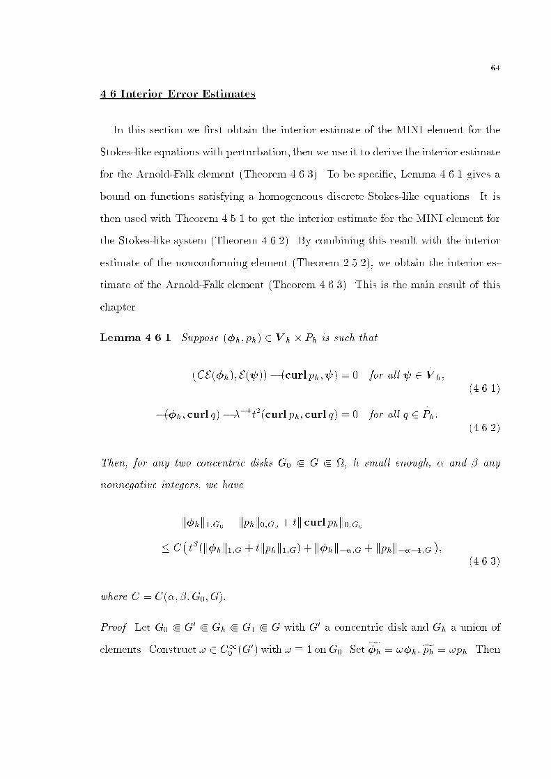
��
�� Interior Error Estimates
In this section we �rst obtain the interior estimate of the MINI element for the
Stokes�like equations with perturbation� then we use it to derive the interior estimate
for the Arnold�Falk element Theorem ������� To be speci�c� Lemma ����� gives a
bound on functions satisfying a homogeneous discrete Stokes�like equations� It is
then used with Theorem ����� to get the interior estimate for the MINI element for
the Stokes�like system Theorem ������� By combining this result with the interior
estimate of the nonconforming element Theorem ������� we obtain the interior es�
timate of the Arnold�Falk element Theorem ������� This is the main result of this
chapter�
Lemma ����� Suppose �h� ph� � V h Ph is such that
CE�h�� E��� � curl ph��� � for all � � V h�������
��h� curl q�� ���t�curl ph� curl q� � for all q � Ph�������
Then� for any two concentric disks G� b G b �� h small enough� � and � any
nonnegative integers� we have
k�hk��G�� kphk��G�
� tk curl phk��G�
� C�t�k�hk��G � tkphk��G� � k�hk���G � kphk�����G
��
������
where C � C�� ��G�� G��
Proof� Let G� b G� b Gh b G� b G with G� a concentric disk and Gh a union of
elements� Construct � � C�� G�� with � � onG�� Set f�h � ��h�fph � �ph� Then
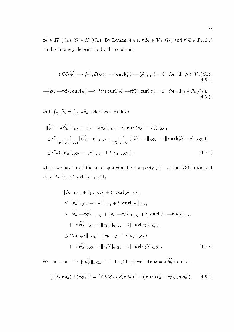
��
f�h � H�Gh�� fph � H�Gh�� By Lemma ������ f�h � V hGh� and fph � PhGh�
can be uniquely determined by the equations
�CEf�h � f�h�� E�� � � �
curlfph � fph��� � � for all � � V hGh��������
�� f�h � f�h� curl q �� ���t�
�curlfph � fph�� curl q � � for all q � PhGh��
������
withRGhfph �
RGh
fph� Moreover� we have
kf�h � f�hk��Gh � kfph � fphk��Gh � tk curlfph � fph�k��Gh
� C�
inf���V h�Gh�
kf�h ��k��Gh � infq�Ph�Gh�
kfph � qk��Gh � tk curlfph � q�k��Gh��
� Ch�k�hk��Gh � kphk��Gh � tkphk��Gh
�� ������
where we have used the superapproximation property cf� section ���� in the last
step� By the triangle inequality
k�hk��G�� kphk��G�
� tk curl phk��G�
� kf�hk��Gh � kfphk��Gh � tk curlfphk��Gh
� kf�h � f�hk��Gh � kfph � fphk��Gh � tk curlfph � fph�k��Gh
� kf�hk��Gh � kfphk��Gh � tk curl fphk��Gh
� Chk�hk��Gh � kphk��Gh � tkphk��Gh�
� kf�hk��Gh � kfphk��Gh � tk curl fphk��Gh� ������
We shall consider kf�hk��Gh �rst� In ������� we take � � f�h to obtain
�CEf�h�� Ef�h� � � �
CEf�h�� Ef�h� �� �curlfph � fph�� f�h �� ������
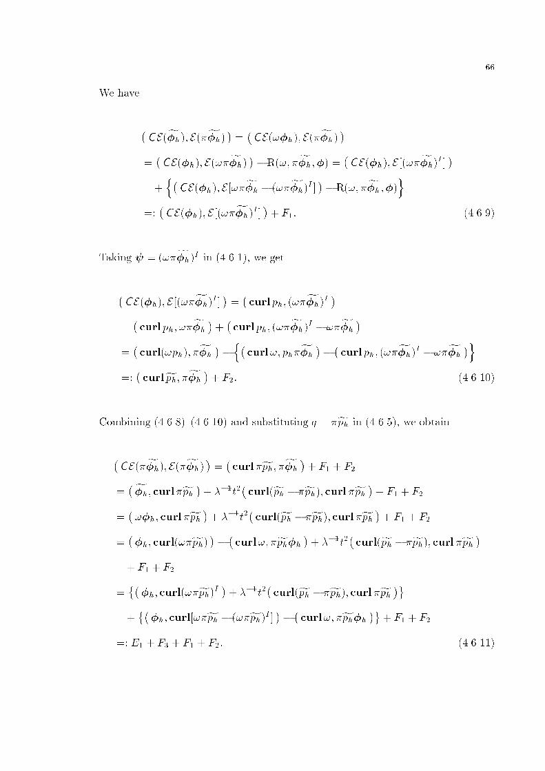
��
We have
�CEf�h�� Ef�h� � � �
CE��h�� Ef�h� ���CE�h�� E�f�h� � �R�� f�h��� � �
CE�h�� E ��f�h�I � ��n�CE�h�� E ��f�h � �f�h�I � ��R�� f�h���o
���CE�h�� E ��f�h�I � �� F�� ������
Taking � � �f�h�I in ������� we get
�CE�h�� E ��f�h�I � � � �
curl ph� �f�h�I ���curl ph� �f�h �� �
curl ph� �f�h�I � �f�h ���curl�ph�� f�h �� n�
curl�� phf�h �� �curl ph� �f�h�I � �f�h �o
���curlfph� f�h �� F�� ������
Combining ������ ������ and substituting q � fph in ������� we obtain
�CEf�h�� Ef�h� � � �
curl fph� f�h �� F� � F�
�� f�h� curl fph �� ���t�
�curlfph � fph�� curl fph �� F� � F�
����h� curl fph �� ���t�
�curlfph � fph�� curl fph �� F� � F�
���h� curl�fph� � � �
curl�� fph�h �� ���t��curlfph � fph�� curl fph �
� F� � F�
����h� curl�fph�I �� ���t�
�curlfph � fph�� curl fph �
����h� curl��fph � �fph�I � �� �
curl�� fph�h � � F� � F�
�� E� � F� � F� � F�� �������

��
Setting q � �fph�I in ������� we get
E� � ����t��curl ph� curl�fph�I �� ���t�
�curlfph � fph�� curl fph �
� ����t��curl ph� curl�fph� �� ���t�
�curl ph� curl��fph � �fph�I � �
� ���t��curlfph � fph�� curl fph �
� ����t�curl�ph�� curl fph� � ���t��curlfph � fph�� curl fph �
�����t�
�curl ph� curl��fph � �fph�I � �� ���t�R��� ph� fph�
�� ����t�curl fph� curl fph� � F�� �������
So far� we have
kC�� Ef�h�k���Gh
� ���t�k curl fphk���Gh� F� � F� � F� � F�� �������
Using the superapproximation properties cf� section ����� the Schwarz inequality�
integration by parts� ������� and ������� we obtain
j F� j� C�hk�hk��Ghkf�hk��Gh � k�hk��Ghkf�hk��Gh
��
j F� j� C�kphk���Ghk
f�hk��Gh � hkphk��Ghkf�hk��Gh
��
j F� j� C�hk�hk��Ghkfphk��Gh � k�hk��Ghkfphk��Gh
��
j F� j� Ct��hk curl phk��Ghkfphk��Gh � kphk��Ghkfphk��Gh
��
Combining the above inequalities with �������� using the inverse inequalities for
fph� �h� and ph� we get
kf�hk���Gh� t�k curl fphk���Gh
� C�hk�hk��Gh � k�hk��Gh � hkphk��Gh � kphk���Gh
�kf�hk��Gh
�C�hk�hk��Gh � k�hk��Gh � t�kphk��Gh
�kfphk��Gh
� C�k�hk��Gh � kphk���Gh
�kf�hk��Gh �C
�k�hk��Gh � t�kphk��Gh
�kfphk��Gh �
�������
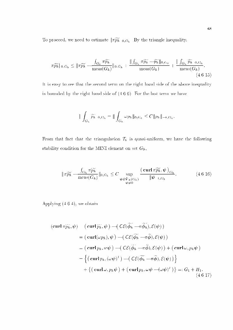
��
To proceed� we need to estimate kfphk��Gh� By the triangle inequality�
kfphk��Gh � kfph � RGh
fphmeasGh�
k��Gh �kRGh
fph �fphk��Gh
measGh��kRGhfphk��Gh
measGh��
�������
It is easy to see that the second term on the right hand side of the above inequality
is bounded by the right hand side of ������� For the last term we have
k
ZGh
fphk��Gh � k
ZGh
�phk��Gh � Ckphk���Gh�
From that fact that the triangulation Th is quasi�uniform� we have the following
stability condition for the MINI element on set Gh�
kfph � RGh
fphmeasGh�
k��Gh � C sup���V h�Gh�
� ��
�curl fph�� �Gh
k�k��Gh
� �������
Applying ������� we obtain
curl fph��� � �curlfph�� �� �CEf�h � f�h�� E�� �
��curl�ph���
���CEf�h � e��� E�� �
��curl ph� w�
���CEf�h � e��� E �� �� �
curl�� ph��
�n�curl ph� ���
I���CEf�h � e��� E�� �o
���curl�� ph�
���curl ph� �� � ���I
� �� G� �H��
�������
��
Setting � � ���I in ������� we get
G� ��CE�h�� E���
I���CEf�h � e��� E �� �
��CE�h�� E���
���CE�h�� E ����
I � ����
��CEf�h � e��� E�� �
�n�
CE��h�� E�����CEf�h � e��� E�� �o
��R�����h� �
�CE�h�� E ����
I � ����
���CEf�h�� E�� � �H�� �������
Applying the superapproximation property� the Schwarz inequlity� ������� �������
and integration by parts� we have
j H� j� C�kphk���Ghk�k��Gh � hkphk��Ghk�k��Gh
��
j H� j� C�k�hk��Ghk�k��Gh � hk�hk��Ghk�k��Gh
��
j Ef�h�� E��� j� kf�hk��Ghk�k��Gh�
Combining ������� ������� �������� the above inequalities� and using the inverse
inequalities� we arrive at
kfphk��Gh
� C�hk�hk��Gh � k�hk��Gh � htkphk��Gh � hkphk��Gh � kphk���Gh� � kf�hk��Gh
� C�k�hk��Gh � htkphk��Gh � kphk���Gh
�� kf�hk��Gh�
�������
Substituting ������� into ������� and using the arithmetic�geometric mean inequal�
ity� we have
kf�hk��Gh � tk curl fphk��Gh � C�k�hk��Gh � t� � ht�kphk��Gh � kphk���Gh
��
������

�
Substituting ������ back into �������� we get
kfphk��Gh � C�k�hk��Gh � kphk���Gh � ht� t��kphk��Gh
�� �������
Hence� combining ������ and ������� with ������� we obtain
k�hk��G�� kphk��G�
� tk curl phk��G�
� C�k�hk��Gh � kphk���Gh � ht� t��kphk��Gh
��
�������
Applying Theorem ����� with G� replaced by G� to bound k�hk��G�and kphk���G�
�
we get
k�hk��G�� kphk��G�
� tk curl phk��G�
� C�hk�hk��G � hkphk��G � tt� h�kphk��G � k�hk���G � kphk�����G
��
Iterating the above inequality � � � times as in section ���� or section ���� but
separating the case h � t with that h � t� we prove ������� �
Theorem ����� Let �� b �� b �� Suppose that �� p� � H� H� satis�es
�j�� �H���� and pj�� � H����� Suppose that �h� ph� � V hPh are such that
CE� � �h�� E��� � curlp� ph���� � F ��� for all � � V h��������
�� ��h� curl q�� ���t�curlp � ph�� curl q� � for all q � Ph��������
for some function F in L�� Let � and � be two arbitrary nonnegative integers�
Then� there is a positive number h� such that for h � � h���
k� � �hk���� � kp� phk���� � tk curlp � ph�k����
� C�kF k���� � hk�k���� � kpk���� � tkpk����� � t�k� ��hk����
� t���kp� phk���� � k�� �hk����� � kp� phk���������
�������

��
for a constant C depending only on ��� ��� �� and ��
Proof� Let G� b G�� b G� b Gh b G� b G be concentric disks and �nd a � �
C�� G�� with � � on G��� Set e� � ��� ep � �p� Then e� � H�Gh�� ep � H�Gh��
By Lemma ������ e� � V hGh�� ep � PhGh� can be de�ned uniquely by the
following equations�
�CE e� � e��� E �� �� �
curlep � ep��� � � F ��� for all � � V hGh���������
�� e� � e�� curl q �� ���t�
�curlep � ep�� curl q � � for all q � PhGh��
�������
withRGh
ep �RGh
ep� Moreover� we have
ke�� e�k��Gh � kep� epk��Gh � tk curlep� ep�k��Gh
� C�
infq�Ph�Gh�
kep� q k ��Gh � tk curlep� q�k��Gh� � kF k��Gh
�� inf���V h�Gh�
ke���k��Gh
�� C
�k�k��G � kpk��G � tkpk��G � kF k��G
�� �������
Let us now estimate k� � �hk��G�� kp � phk��G�
� and tk curlp � ph�k��G�� By the
triangle inequality� we have
k�� �hk��G�� kp� phk��G�
� tk curlp� ph�k��G�
� k�� e�k��G�� kp� epk��G�
� k e�� �hk��G�� kep� phk��G�
� tk curlp � ep�k��G�� tk curlep� ph�k��G�
� �������
Since �������� ������� and �������� ������� hold for any � � V hG����
��
q � PhG���� respectively� Subtracting the corresponding two equations� we obtain
E �h � e��� E��� � curlph � ep���� � for all � � V hG����
������
��h � e�� curl q�� ���t�curlph � ep�� curl q� � for all q � PhG�����������
Then we apply Lemma ����� to �h � e� and ph � ep with G replaced by G�� to
obtain
k�h � e�k��G�� kph � epk��G�
� tk curlph � ep�k��G�
� C�t�k�h � e�k��G�� � t���kph � epk��G�� � k�h � e�k���G��
� kph � epk�����G�� �� C
�t���kp� epk��G�� � t���kph � pk��G��
� k� � e�k���G�� � k�h � �k���G��
� t�k�� �hk��G�� � t�k�h � �hk��G�� � kp� epk�����G
�
�� kp� phk�����G��
�� C
�ke�� e�k��Gh � kep� epk��Gh � tk curlep � epk��Gh
� t�k�� �hk��G � t���kp� phk��G � k� � �hk���G � kp� phk�����G���������
Combining �������� �������� and �������� we obtain
k�� �hk��G�� kp� phk��G�
� tk curlp� ph�k��G�
� C�kF k��G � k�k��G � kpk��G � tk curl pk��G
� t�k� ��hk��G � t���kp� phk��G � k�� �hk���G � kp� phk�����G��
Since ��� q�� �h � q�� and �p� q�� ph � q�� also satisfy equations ������� and
������� for any � � V h and q � Ph� we have
k�� �hk��G�� kp� phk��G�
� tk curlp� ph�k��G�
� C�
inf���V h
k� ��k��G � infq��Ph
kp � qk��G � tk curlp � q�k��G� � kF k��G
� k� � �hk���G � kp� phk�����G � t�k�� �hk��G � t���kp� phk��G��
��
Then� �rst using the approximation properties of the �nite element spaces and then a
covering argument cf� section ��� and section ����� we obtain the desired result� �
We now state the main result of this chapter�
Theorem ����� Let �� b �� b � and suppose that r��� p� w� � H�H�H�
H� the exact solution satis�es r��� p� w�j�� � H���� H���� H����
H����� Suppose that rh��h� ph� wh� � Wh V h Ph Wh the �nite element
solution is given so that ������� ������� ������� and ������ hold� Let �� � be
two nonnegative integers� Then there exists a positive number h� and a constant C
depending only on ��� ��� �� and �� such that for all h � � h��
kr � rhkh����
� C�hkrk���� � kr � rhk�����
��������
k� � �hk���� � kp� phk���� � tk curlp � ph�k����
� C�hk�k���� � kpk���� � tkpk���� � krk���� � � kr � rhk�����
� k� ��hk����� � kp� phk������� � t�k� � �hk���� � t���kp� phk������
�������
kw � whkh����
��Chk�k���� � kpk���� � tkpk���� � krk���� � kwk�����
� kw � whk����� � k� � �hk����� � kr � rhk�����
� kp� phk������� � t�k�� �hk���� � t���kp� phk������ �������
Proof� Find a subdomain �� such that �� b �� b ��� Apllying Theorem ����� with
�� replaced by �� yields
kr � rhkh���� � C
�hkrk���� � kr � rhk�����
�� �������
which also implies �������� From ������� ������� �������� and Theorem ����� with
��
�� replaced by ��� we obtain
k�� �hk���� � kp� phk���� � tk curlp� ph�k����
� C�hk�k���� � kpk���� � tkpk����� � kgradhr � rh�k����
� k�� �hk����� � kp� phk������� � t���kp� phk���� � t�k� ��hk�����
� C�hk�k���� � kpk���� � tkpk���� � krk���� � � k�� �hk�����
� kp� phk������� � t�k� � �hk���� � t���kp� phk���� � kr � rhk�������
This completes ��������
We now consider the interior estimate for the transverse displacement� Because
of the di�erence between ������ required by Theorem ������� and ������ satis�ed
by w � wh��� Theorem ����� cannot be used directly� But we can follow the same
proof to get ��������
Let G� b G� b G be concentric disks and Gh be a union of triangles which
satis�es G� b Gh b G� Use the notation ew � �w and de�ne ew � �WhGh� by
gradh ew�gradh s� � gradh ew�gradh s� for all s � �WhGh��
We have
k ew � ewkh��Gh� C inf
s� Wh�Gh�k ew � sk��Gh � C hkwk��Gh�
By the triangle inequality�
kw � whkh��G�
� k ew � ewkh��Gh� k ew � whk
h��G�
� Chkwk��Gh � k ew � whkh��G�
� �������
From ������ and the fact that � � � on G��
gradh ew � wh��gradh s� � gradhw � wh��gradh s�
� Ls� for all s � WhG����������
��
where
Ls� �� � � �h � ���t� gradhr � rh��gradh s� �XT�Th
Z�T
� � nT � ���t��r
�n�s�
for all s � Wh� By Lemma ������
jLs�Gh j � C�k� � �hk��Gh � kr � rhk
h��Gh
� hk�k��Gh � krk��Gh��kgradh sk��Gh for all s � WhGh��
which implies
kLkGh � C�k�� �hk��Gh � kr � rhk
h��Gh
� hk�k��Gh � krk��Gh���
Under ������� we apply Lemma ����� with G replaced by G� to obtain
k ew � whkh��G�
� C�k ew � whk�t�G�
� kLkG��
� Ck ew� ewk�t�Gh � kw �whk�t�G�� kLkGh�
� C�k�� �hk��G� � kr � rhk
h��G� � kw � whk���G
� hk�k��G � krk��G���
�������
Using the triangle inequality� �������� and ������� yields
kw � whkh��G�
� C�k�� �hk��G� � kr � rhk
h��G� � kw � whk���G
� hk�k��G � kwk��G � krk��G���
Applying ������� and ������� with �� and �� replaced by G� and G� respectively�
we obtain a local version of �������� Then a standard covering argument leads to
�������� �

��
��� The Global and Interior Convergences of the ArnoldFalk Element
As an application of the theory we developed in the last section� we consider the
soft simply supported plate with a smooth forcing function g� Under this boundary
condition for a smooth ��� the exact solution of the Reissner�Mindlin plate satis�es
cf� ����
krk� � kwk� � k�k��� � kpk��� � tkpk��� � C�
k�k����� � kpk����� � tkpk����� � C�t���
k�k� � kpk� � tkpk� � Ct�����
������
for a constant C� that is independent of t and h� and � � � ����� Obviously�
functions � and p are not regular enough to ensure that the MINI element converges
at the optimal rate� uniformly in the plate thickness t�
Thus� we want to use Theorem ����� to obtain the interior convergence rates
of the Arnold�Falk element� To do so� we must estimate kp � phk�� k� � �hk��
kr � rhk����� � k� � �hk����� � kp � phk������� � and kw � whk����� for some
suitable domain �� and integer �� The only way of doing these� as far as we
know� is to use the inequality k � kt��� � k � kt��� Hence� the global convergence of
the nonconforming element for the Poisson equation and that of the MINI element
for the Stokes�like equations must be established� The �rst one is well�known but
the second one is di�cult due to the special structure of the singularly perturbed
Stokes�like equations and the type of the boundary condition imposed� Because of
the di�culty in dealing with the boundary approximation when the boundary layer
exists� we will only work on a polygonal domain� i�e�� we will assume that � is a
convex polygon� Therefore� we need to know the regularity of the exact solution
of the singularly perturbed generalized Stokes�like equations on a convex polygon
under the soft simply supported boundary condition�� But so far we cannot prove
��
the regularity result Theorem ������ we need� So we will assume that it is true� We
feel that we have reason to believe it is correct possibly with some restriction on
the magnitude of the maximum angle of the polygon�� As a partial justi�cation� we
will prove a similar result for a smooth � in Appendix B�
This section is organized as follows� Theorem ����� presents a technical result on
the approximation property of the continuous piecewise linear functions� Its proof
can be found in Appendix A� Theorem ����� is the assumption we just mentioned�
The global convergence of the Arnold�Falk element is given in Theorem ������ Finally
by combing Theorem ����� and Theorem ����� we get the interior convergence rate
of the Arnold�Falk element for the rotation Theorem �������
Theorem ������ Let � be a convex polygon and u � H�� Then there exists an
operator h � H� � Ph such that
kp� hpk� � C�h�����kpk������ ������
kp� hpk� � Ch���kpk���� ������
kp� hpk������� � C�h�����kpk������ ������
for any � � � ���� Here C is independent of � and C� depends on �� but not h�
Proof� See Theorem ������ Appendix A�
Theorem ������ Let � be a convex polygon and F �H� and K � H� � #L�� Then
there exists a unique solution �� P � �H� H� � #L� to the equations
CE��� E��� � �� curlP � � F ��� for all � �H��������
��� curlQ� � ���t�curlQ� curl P � � K�Q� for all Q � H��������

��
Moreover�
k�k����� � kPk����� � tkPk����� � C�t���kF k� � t���kF k�
�for K � �
������
k�k����� � kPk����� � tkPk����� � C�t��kKk� for F � � ������
for � � � ����
Proof� See Corollary ���� Appendix B�
Theorem ������ Let � be a convex polygon� Assume that r��� p� w� and
rh��h� ph� wh� solve ������������� and �������������� respectively� for some
smooth g� some t � � ��� and a quasi�uniform mesh Th� Then�
k� ��hk� � kp� phk� � tk curlp� ph�k� � C�h���t��� ������
k� ��hk� � kw � whkh� � C�ht
��� ������
tk� ��hk� � t�k curlp � ph�k� � Ch� �������
k� ��hk�� � kp� phk�� � C�ht��� �������
for an arbitrarily small constant ��
Proof� Subtracting ������ by ������ and ������ by ������� respectively� we obtain�CE� � �h�� E ��
����� curlp� ph�
���gradr � rh���
�for all � � V h
�������
��curl q�� � �h
�� ���t�
�curlp� ph�� curl q
�� for all q � Ph
�������
From ������� and ������� see also the proof on page ���� of ��� Theorem ������
we have
kC�� E�h ���k
�� � ���t�k curlph � q�k��
��CE� ���� E�h ���
�� ���t�
�curlp � q�� curlph � q�
���curlp� q���h ��
������� curlph � q�
���gradhrh � r���h ��
��
�������
��
In the above we choose � to be the Fortin projection of �� that is�
� � �� curl q� � for all q � Ph�
k�� �k� � Ck���k� for all � � V h�
We see that the fourth term on the right hand side of ������� is gone� Taking
q � hp to be the interpolant of p described in Theorem ����� and using the Schwartz
inequality� integration by parts� and the arithmetic�geometric mean inequality� we
obtain
kC�� E�h � ��k
�� � ���t�k curlph � hp�k
��
� Ck�� �k�� � t�kp� hpk�� � kp� hpk�k rot�h � ��k�
� k�h � �k�kp� hpk������� � hk�h � �k��� �������
To estimate k�h� �k�� we note that theH� norm of the vector function �h� �
is equivalent to
kE � ��h�k� � j
Z � � �hj� j
Z �� �h� � �y� x�j� �������
The �rst term in ������� is already covered by �������� To control the other two�
we take q � y and q � x� respectively in ������� to get
j
Z� ��h�j � Ct�j
Zcurlp� ph�j�
which implies
j
Z �� �h�j � j
Z � ���j � Ct�k curlp � ph�k�
� C�k� � �k� � t�k curlp � hp�k� � t�k curlhp� ph�k�
���������
�
To control the third term in �������� we take q � Lhq� � Lhx� � y����� the L�
projection of x� � y���� in Ph�� in �������� to obtain
�� � �h� curl q�
���� � �h� curlq� � Lhq��
�� ���t�
�curlp � ph�� curlLhq�
��
Using the fact that
kq� � Lhq�k��� � Ch
and
kLhq�k��� � C�
we obtain
j
Z� ��h� � �y� x�j � C
�hk�� �hk� � t�j
Zcurlp� ph�j
�� �������
Therefore�
j
Z � ��h� � �y� x�j
� C�k�� �k� � hk � � �hk� � t�k curlp � hp�k� � t�k curlhp� ph�k�
��
������
Combining ������� ������ and using the arithmetic�geometric mean inequality� we
get
k�h � �k� � tk curlph � hp�k�
� C�k�� �k� � tkp� hpk� � kp� hpk� � kp� hpk������� � h
��
Applying the approximation property of and Theorem ������ we get
k�h � �k� � tk curlph � hp�k�
� C�h����k�k��� � tkpk��� � kpk����� � h���
��
��
which implies
k�� �hk� � tk curlp� ph�k� � C�h���t��� �������
Moreover�
tk�� �hk� � t�k curlp � ph�k� � Ct�k�� �k� � tkp� hpk�
� kp� hpk������� � h�
� Cth�k�k� � tkpk� � �
�� Ch�
To estimate kp�phk�� we simply repeat the proof on page ���� of ��� Theorem �����
By the stability condition� there exits � � independent of h such that for all q � #Wh
there exists a nonzero � � V h with
�kqk�kgrad�k� � curl q����
Applying this result with q replaced by ph �hp�R�hp�� and again using ������
and ������� we have
�kph � hp�
Z�
hpk�kgrad�k� ��curlph � hp���
���curlp � hp���
���CE�h � ��� E ��
���gradhrh � r���
�� C
�kp� hpk� � kgrad�h � ��k� � kgradhrh � r�k�
�kgrad�k��
so
kph � hp �
Z�
hpk� � C�kp� hpk� � k�� �hk� � kgradhr � rh�k�
��
By the triangle inequality� we get
kp� phk� � C�kpk� � kp� hpk� � k� ��hk� � kgradhr � rh�k�
��

��
Since if � � �h� p � ph� satis�es ������� and �������� so will
�� � �� � �h � ��� p � q� � ph � q��� for any �� q� � V h Wh� Therefore�
together with ������� and Theorem ������ we get
kp� phk� � C�kp� hpk� � k�� �hk� � kgradhr � rh�k�
�� C�h
���t���
This completes ������� To bound k� � �hk�� we construct the following duality
problem�
Find �� P � �H� #H� such that
CE��� E��� � �� curlP � � �� �h��� for all � �H���������
�curl q��� � ���t�curl q� curlP � � for all q � H�� �������
From Corollary ����� we know that �� P � is uniquely de�ned� Moreover�
k�k����� � kPk����� � tkPk����� � C�t���k�� �hk� � t���k���hk�
��������
Following the proof of Theorem ��� on page ���� of ���� we can obtain� for q��� �
hP� ��� where is the Fortin projection and h the interpolant as described in
Theorem ������
k� ��hk�� �
�CE� � �h�� E� � ��
����� �h� curlP � hP �
���curlp � hp��� � �
�� ���t�
�curlp� ph�� curlP � hP �
���gradhr � rh�� �
���CE� � �h�� E� � ��
���rot� ��h�� P � hP
�� h� ��h� � s� P � hP i�� �
�p� hp� rot�� ��
�� hp� hp� � � �� � si�� � ���t�
�curlp � ph�� curlP � hP �
���gradhr � rh�� �
��������
��
Using the Schwartz inequality and integration by parts in �������� we get
k�� �hk��
� Ck�� �hk�k�� �k� � kP � hPk� � kP � hPk��������
� k�� �k�kp � hpk� � kp� hpk��������
� t�k curlp � ph�k�k curlP � hP �k� � kgradhr � rh�k�k �k���������
If t � h� then by Theorem ������ �������� �������� and ������� we obtain
k� � �hk��
� C�ht���k�k��� � kPk�����
�� Chk�k���kpk����� � C�hkPk��� � Chk�k�
� C�ht���
�k�� �hk� � t���k� ��hk�
�� C�ht
����k�� �hk� � h�
��
which implies
k� ��hk� � C�ht����
If t � h� using ������� with � � ��� in �������� we obtain
k�� �hk��
� C�h���t��k�k� � kPk�� � C�h
���t��k�k� �C�h���t��kPk� � Chk�k�
� C�h���t��t����k� � �hk� � t���k� ��hk�� � Chk���hk��
Since t � h�
k�� �hk�� � C�ht
��k� ��hk� � h���
Hence
k� ��hk� � C�ht���
��
To analyze w �wh� we follow that in ���Theorem ����� De�ne ��h � �Wh by
�gradh �wh�gradh s
����� ���t� grad r�gradh s
�for all s � �Wh�
So
kw � �whkh� � Ch
�k� � t�rk� � kwk�
�� Ch�
where we use the fact that k�k� � krk� � kwk� � C� with C independent of t� In
addition� we have
�gradh �wh � wh��gradh s
���� ��h � ���t� gradhr � rh��gradh s
��
for all s �Wh� Obviously�
k �wh � whkh� � C
�k�� �hk� � t�kgradhr � rh�k�
�� C
�h� k�� �hk�
��
which implies
kw � whkh��� � kw � �whk
h� � k �wh � whk
h� � Ch� k� � �hk�� � C�ht
���
This completes �������
We will use the duality argument again to estimate kp � phk��� To do so� we
introduce the following auxiliary problem�
Find �� P � �H� #H� such that
CE��� E��� � �� curlP � � for all � �H�� �������
�curl q��� � ���t�curl q� curlP � � K� q� for all q � H�� ������
for any K � #L�� By Corollary ������ this problem admits a unique solution� and
that
k�k����� � kPk����� � tkPk����� � C�t��kKk�� �������
��
By de�nition�
kp� phk�� � supK��H�
K ��
p � ph�K�
kKk�� �������
In ������� we take q to be p� ph and apply ������� ������� ������� ������� and
������� to obtain
p � ph�K� ����� �� curlp� ph�
�� ���t�
�curlp � ph�� curlP � hP �
���CE� � �h�� E� � ��
����� �h� curlhP � P �
���gradhr � rh�� �
��������
Using the Schwartz inequality� Theorem ������ and ������� in �������� we get
jp� ph�K�j � C�ht���k�k��� � tkPk��� � kPk�����
�� �������
Combining ������� �������� we arrive at
kp� phk�� � C�ht����
Similarly� we can prove
k�� �hk�� � C�ht����
Since � is an arbitrary number� then ������� is proved� �
Equipped with the above result� we are able to prove the following interior esti�
mate for the Arnold�Falk element for the rotation ��
Theorem ������ Let � be a convex polygon and ��� b � an interior domain� Let g
be a smooth function� Assume that Th is quasi�uniform� Suppose that w��� solves
������ and wh��h� solves ������� Then there exists a number h� � � such that
for all h � � h���
k� ��hk���� � C� ht��� �������
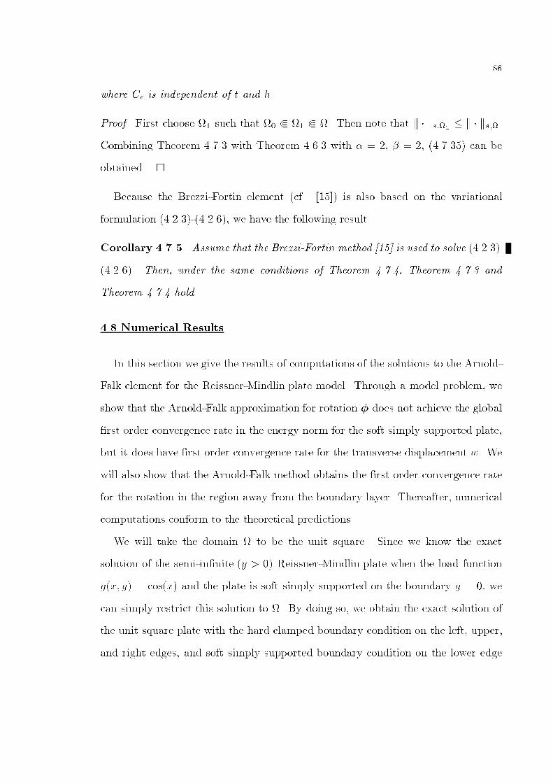
��
where C� is independent of t and h�
Proof� First choose �� such that �� b �� b �� Then note that k � ks��� � k � ks���
Combining Theorem ����� with Theorem ����� with � � �� � � �� ������� can be
obtained� �
Because the Brezzi�Fortin element cf� ����� is also based on the variational
formulation �������������� we have the following result�
Corollary ������ Assume that the Brezzi�Fortin method ��� is used to solve �������
������� Then� under the same conditions of Theorem ������ Theorem ����� and
Theorem ����� hold�
��� Numerical Results
In this section we give the results of computations of the solutions to the Arnold�
Falk element for the Reissner�Mindlin plate model� Through a model problem� we
show that the Arnold�Falk approximation for rotation � does not achieve the global
�rst order convergence rate in the energy norm for the soft simply supported plate�
but it does have �rst order convergence rate for the transverse displacement w� We
will also show that the Arnold�Falk method obtains the �rst order convergence rate
for the rotation in the region away from the boundary layer� Thereafter� numerical
computations conform to the theoretical predictions�
We will take the domain � to be the unit square� Since we know the exact
solution of the semi�in�nite y � � Reissner�Mindlin plate when the load function
gx� y� � cosx� and the plate is soft simply supported on the boundary y � � we
can simply restrict this solution to �� By doing so� we obtain the exact solution of
the unit square plate with the hard clamped boundary condition on the left� upper�
and right edges� and soft simply supported boundary condition on the lower edge
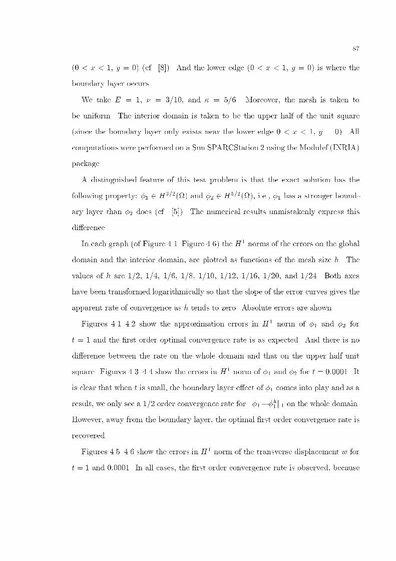
��
� x � �� y � � cf� ����� And the lower edge � x � �� y � � is where the
boundary layer occurs�
We take E � �� � � ���� and � � ���� Moreover� the mesh is taken to
be uniform� The interior domain is taken to be the upper half of the unit square
since the boundary layer only exists near the lower edge � x � �� y � �� All
computations were performed on a Sun SPARCStation � using the Modulef INRIA�
package�
A distinguished feature of this test problem is that the exact solution has the
following property� �� � H����� and �� � H ����� i�e�� �� has a stronger bound�
ary layer than �� does cf� ����� The numerical results unmistakenly express this
di�erence�
In each graph of Figure ��� Figure ���� the H� norms of the errors on the global
domain and the interior domain� are plotted as functions of the mesh size h� The
values of h are ���� ���� ���� ���� ���� ����� ����� ���� and ����� Both axes
have been transformed logarithmically so that the slope of the error curves gives the
apparent rate of convergence as h tends to zero� Absolute errors are shown�
Figures ��� ��� show the approximation errors in H� norm of �� and �� for
t � � and the �rst order optimal convergence rate is as expected� And there is no
di�erence between the rate on the whole domain and that on the upper half unit
square� Figures ��� ��� show the errors in H� norm of �� and �� for t � ��� It
is clear that when t is small� the boundary layer e�ect of �� comes into play and as a
result� we only see a ��� order convergence rate for k����h�k� on the whole domain�
However� away from the boundary layer� the optimal �rst order convergence rate is
recovered�
Figures ��� ��� show the errors in H� norm of the transverse displacement w for
t � � and ��� In all cases� the �rst order convergence rate is observed� because
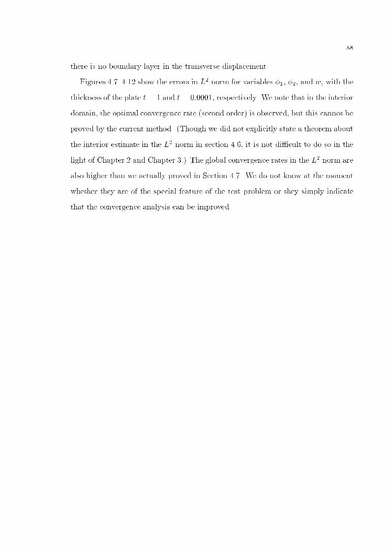
��
there is no boundary layer in the transverse displacement�
Figures ��� ���� show the errors in L� norm for variables ��� ��� and w� with the
thickness of the plate t � � and t � ��� respectively� We note that in the interior
domain� the optimal convergence rate second order� is observed� but this cannot be
proved by the current method� Though we did not explicitly state a theorem about
the interior estimate in the L� norm in section ���� it is not di�cult to do so in the
light of Chapter � and Chapter ��� The global convergence rates in the L� norm are
also higher than we actually proved in Section ���� We do not know at the moment
whether they are of the special feature of the test problem or they simply indicate
that the convergence analysis can be improved�

��
10-2
10-1
100
101
10-2 10-1 100
o
o
o
oo
o
oo
o
x
x
x
xx
x
xx
x
t=1
o--Global
x--Interior
1
Figure ���� Errors in H� Norm for ��
10-2
10-1
100
101
10-2 10-1 100
o
o
o
oo
o
oo
o
x
x
x
xx
x
xx
x
t=1
o--Global
x--Interior
1
Figure ���� Errors in H� Norm for ��

�
10-2
10-1
100
101
10-2 10-1 100
o
oo
oooo
oo
x
x
x
xx
x
xx
x
t=0.0001
o--Global
x--Interior
1
0.5
Figure ���� Errors in H� Norm for ��
10-2
10-1
100
101
10-2 10-1 100
o
o
o
oo
o
oo
o
x
x
x
xx
x
xx
x
t=0.0001
o--Global
x--Interior
1
Figure ���� Errors in H� Norm for ��

��
10-2
10-1
100
10-2 10-1 100
o
o
o
o
oo
o
oo
x
x
x
x
x
x
x
xx
t=1
o--Global
x--Interior
1
Figure ���� Errors in H� Norm for w
10-2
10-1
100
10-2 10-1 100
o
o
o
o
o
o
o
oo
x
x
x
x
x
x
x
xx
t=0.0001
o--Global
x--Interior
1
Figure ���� Errors in H� Norm for w
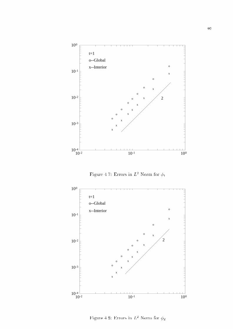
��
10-4
10-3
10-2
10-1
100
10-2 10-1 100
o
o
o
o
oo
o
oo
x
x
x
x
xx
x
x
x
t=1
o--Global
x--Interior
2
Figure ���� Errors in L� Norm for ��
10-4
10-3
10-2
10-1
100
10-2 10-1 100
o
o
o
o
oo
o
oo
x
x
x
x
x
x
x
xx
t=1
o--Global
x--Interior
2
Figure ���� Errors in L� Norm for ��

��
10-4
10-3
10-2
10-1
100
10-2 10-1 100
o
o
o
oo
o
oo
o
x
x
x
x
xx
x
xx
t=0.0001
o--Global
x--Interior
2
1.5
Figure ���� Errors in L� Norm for ��
10-4
10-3
10-2
10-1
100
10-2 10-1 100
o
o
o
o
oo
o
oo
x
x
x
x
x
x
x
x
x
t=0.0001
o--Global
x--Interior
2
Figure ���� Errors in L� Norm for ��

��
10-4
10-3
10-2
10-1
10-2 10-1 100
o
o
o
o
o
o
o
o
o
x
x
x
x
x
x
x
x
x
t=1
o--Global
x--Interior
2
Figure ����� Errors in L� Norm for w
10-4
10-3
10-2
10-1
10-2 10-1 100
o
o
o
o
o
o
o
o
o
x
x
x
x
x
x
x
x
x
t=0.0001
o--Global
x--Interior
2
Figure ����� Errors in L� Norm for w

��
APPENDIX A
AN APPROXIMATION RESULT
��� Introduction
The purpose of this appendix is to prove Theorem ������ which is due to Arnold ����
This approximation result was used extensively in Chapter � as Theorem ������ for
proving the global convergence of the Arnold�Falk element for the Reissner�Mindlin
plate model under the simply supported boundary condition�
Recall that Ph is the space of continuous piecewise linear functions� We shall
start with a result by Scott and Zhang �����
Theorem ������ Assume that � is a convex polygon� Let % � �� and P�h �
f vj� � v � Ph g � H�%�� There exists a projection Ih � H� � Ph such that if
uj� � P�h then Ihuj� � uj�� Moreover
ku� Ihuks � Chl�skukl� for � s � l � �� l � ���� ������
Using this� we can quickly prove�
Lemma ������ Let w � H� be a function for which wj� � P�h � De�ne wh � Ph byZ
�
gradwh � gradv �
Z�
gradw � gradv for all v � Ph� wh � w on %�
Then
kw � whk� � C inf��Ph
�w on �
kw � �k�� ������
kw � whk� � Chkw� whk�� ������
kw �whks � Cht�skwkt� s � � �� t � �� �� ������
��
Proof� The �rst two estimates are completely standard� We take � to be the inter�
polant of Theorem ����� to get the third� �
The outline of this chapter is as follows� Section ��� constructs the approximation
operator and section ��� proves that it has the desired property�
��� The Construction of the Approximation Operator
In this section we study a �nite element method for the nonhomogeneousDirichlet
problem for the Poisson equation� We will prove some of the properties of the �nite
element method here and we will show in the next section that the approximation
operator determined by the �nite element solution is the one we need�
For simplicity� we will use notation j � jt to denote k � kt��� in this chapter instead
of its old meaning as the semi�norm on Ht��
Lemma ������ Given p � H�� let g � pj� and let gh be the L�%��projection of g
into P�h � De�ne ph � Ph by
Z�
gradph �grad q �
Z�
grad p �gradq for all q � Ph� ph � gh on %� ������
Then
kp� phks � Cht�skpkt� � s � �� � � t � ��
Proof� De�ne �ph � H� by
� �ph � � p in �� �ph � gh on %�
Since p� �ph is harmonic� we have
kp� �phk� � Cjg� ghj����� kp� �phk� � Cjg � ghj���� ������

��
Now using a standard duality argument and standard approximation results for the
L��projection into P�h together with the trace theorem we get
jg � ghj���� � supf�H������
hg � gh� fi
jf j���
� supf�H������
hg � gh� f � fI i
jf j���
� Ch���jg � ghj� � Chjgj��� � Chkpk�� ������
where fI is the L�%� projection of f on P�h � Although % is not su�ciently smooth
to de�ne the space H���%� intrinsically� we can de�ne �H���%� to be the space
of functions in H�%� whose restrictions to each edge e of the polygon belong to
H���e�� and use as the norm
v��� ��
�Xe���
kvk�H����e�
����
�
Then
jg � ghj���� � Ch���jg � ghj� � Ch�jgj��� � Ch�kpk�� ������
From jg � ghj� � Cjgj� and the inverse inequality we can obtain jg � ghj� � Cjgj��
Then� by the interpolation theorem we get
jg � ghj��� � Cjgj��� � Ckpk�� jg � ghj��� � Chjgj��� � Chkpk�� ������
Combining ������ ������ we get
kp� �phks � Cht�skpkt� s � � �� t � �� �� ������
NowZ�
grad ph � grad q �
Z�
grad �ph � grad q for all q � Ph� ph � �ph on %�
��
Then� using ������ in the case t � � we obtain
k�ph � phks � Ch��sk�phk�� s � � ��
Thus combining the above with ������ in the case t � � we get
kp� phks � Ch��skpk� � k�phk�� � Ch��skpk�� s � � ��
where in the last step we use ������ for s � � and t � ��
Now let Ihp be the usual piecewise linear interpolant of p so that egh �� Ihpj� is
the piecewise linear interpolant of g� and de�ne eph � Ph by
Z�
grad eph � grad q � Z�
gradp � grad q for all q � Ph� eph � egh on %�
Then
kp� ephk� � C inf��Ph
�egh on �
kp� �k� � Ckp� Ihpk� � Chkpk�� ������
Next� de�ne w � H� by
�w � in �� w � egh � gh on %�
Note that eph � ph � Ph� and
Z�
gradeph � ph� � grad q �
Z�
gradw � grad q � for all q � Ph�
eph � ph � w on %�
Then by the Lemma ������ we have keph � phks � Ch��skwk�� for s � � �� Since
kwk� � Cjegh � ghj��� � Cjg � eghj��� � jg � ghj���� � Chjgj��� � Chkpk��
��
we get
keph � phks � Ch��skpk��
which� together with ������ gives kp� phk� � Chkpk��
Finally we use duality to prove that kp�phk� � Chkp�phk�� and thus kp�phk� �
Chkpk�� Namely� we de�ne z by
�� z � p� ph in �� z � on %�
Then kzk� � Ckp� phk�� and
kp� phk�� � �
Z�
p � ph�� z �
Z�
gradp� ph� � grad z �
Z�
g � gh��z
�nT
� kp� phk� inf���Ph
kz � �k� � jg � ghj����
���� �z�nT
�������
� Chkp� phk�kzk� � Ch�jgj���kzk�
� Ch�kpkkp� phk��
as desired�
This completes the proof for s � and �� and t � � and �� The extension to real
indices follows by interpolation� �
��� The Main Result
For p � H�� let hp � ph be the �nite element solution de�ned in Lemma ������
In the following� we shall prove that h is what we need� To do so� we should keep
in mind two important properties of h� equation ������ and that h preserves P�h
on the boundary�

�
Theorem ������ Assume that u � H�� where � is a convex polygon� Then the
operator h � H� � Ph constructed in Lemma ����� satis�es
kp� hpk� � C�h�����kpk������ ������
kp� hpk� � Ch���kpk���� ������
jp� hpj���� � C�h�����kpk������ ������
for any � � � ���� Here C is independent of � and C� depends on �� but not h�
Proof� Inequality ������ is already proved in Lemma ������ Inequality ������ is
also straightforward� since hp is the L�%� projection of p on P�h � we have
jp� hpj���� � Ch���jp� hpj� � C�h�����jpj� � C�h
�����kpk������
where we use the trace theorem in the last step�
We now prove ������ in three steps� �rst for p � H�� then for p such that
pj� � P�h � and �nally for all p � H��
Using an inverse inequality ����Theorem ����� we obtain
kzhk����� � C�h������kzhk� for all zh � Ph�
which implies that zh � H������ For all T � Th� applying inequality ����
kuk��s�T � C kuk��T � �s����s�kuk��T �
for u � z � hz� � h������ and s � ���� � yields
kz� hzk������T � C�h�����kz� hzk��T � h������kz� hzk��T � for all z � H��
Summing up inequalities of above type for all T � � and noting that the second
order derivative of hz vanishes� we obtain
kz � hzk����� � C�h�����kzk� � h������kz � hzk�� for all z � H���

��
Then applying Lemma ����� for s � � and t � � yields
kz � hzk����� � C�h�����kzk� for all z � H�� ������
Now if p � H� then hp � Ph� so if both p� z � H��
gradhp�grad z� � gradhp�gradhz� � gradp�gradhz��
For a given p � H�� we will use a duality argument to get ������� Taking z � H�� H�
with �� z � p�hp and kzk� � Ckp�hpk� for hz as described in Lemma ������
we get
kp� hpk�� � gradp � hp��grad z� � gradp�gradz � hz��
� kgradpk�����kgradz � hz�k����� � kpk�����kz � hzk�����
� C�h�����kpk�����kzk� � C�h
�����kpk�����kp� hpk��
which proves ������ for p � H��
Assume p � H� has the property that pj� � P�h � Let Ih denote the Scott�Zhang
interpolant ����� Then� since Ihp � p on % and� using what we just proved and the
fact that Ih is bounded in H������ we obtain
kp� hpk� � kp� Ihp� � hp� Ihp�k�
� C�h�����kp� Ihpk����� � C�h
�����kpk������
This completes the proof of the second case� Finally for the general case of p � H�
we use the same decomposition as in the proof of Lemma ������ Namely we de�ne
�ph � H� by
� �ph � � p in �� �ph � gh on ���
where gh is the L�%��projection of g � pj� into P�h � Then
kp� �phk� � jg � ghj���� � C�h�����jgj� � C�h
�����kpk������
��
Also
kp� �phk����� � jg � ghj� � C�jgj� � C�kpk������
Here we have used an inverse inequality to obtain that the L�����projection is
bounded in H����� We thus have
k�phk����� � C�kpk������
Finally we have h �ph � hp� so
k�ph � hpk� � k�ph � h�phk� � C�h�����k�phk����� � C�h
�����kpk������
This completes the proof� �

��
APPENDIX B
A REGULARITY RESULT
The purpose of this Appendix is to prove Theorem ��� on the regularity of the
exact solution of the singularly perturbed Stokes�like system under the soft simply
supported boundary condition� This is done assuming that the domain � is smooth�
So far� we cannot prove the same result for a convex polygonal domain�
Theorem ��� Let � denote a smooth domain� and let F �H� and K � H� � #L��
Then there exists a unique solution �� P � �H� H� � #L� to the equations
CE��� E��� � �� curlP � � F ��� for all � �H������
��� curlQ� � ���t�curlQ� curl P � � K�Q� for all Q � H������
Moreover�
k�k� � kPk� � tkPk� � C�t����kF k���� � kKk���� � tkF k� � kKk��
������
kPk��� � C�kF k���� � kKk��� � tkF k��� � kKk����
�� ����
k�k��� � tkPk��� � C�kF k���� � kKk��� � t���kF k� � kKk��
�� ����
Proof� We �rst de�ne some notations� Let
Mn� �� n � CE��n � D
���
�n� n� �
��
�s� s
��
Ms� �� s � CE��n �D� � ��
�
���
�n� s � �
��
�n� n
��
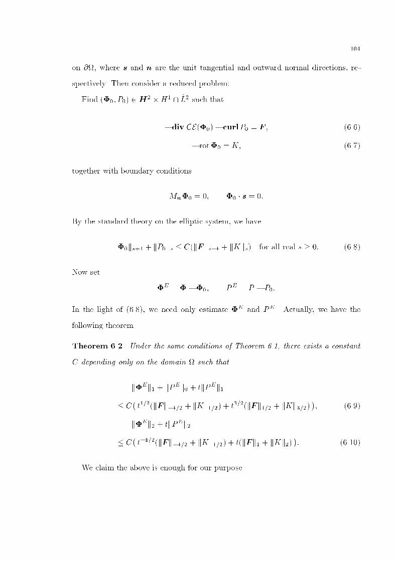
��
on ��� where s and n are the unit tangential and outward normal directions� re�
spectively� Then consider a reduced problem�
Find ��� P�� � H� H� � #L� such that
�div CE���� curlP� � F � ����
� rot�� � K� ����
together with boundary conditions
Mn�� � � �� � s � �
By the standard theory on the elliptic system� we have
k��ks�� � kP�ks � CkF ks�� � kKks� for all real s � � ����
Now set
�E � � ���� PE � P � P��
In the light of ����� we need only estimate �E and PE� Actually� we have the
following theorem�
Theorem ��� Under the same conditions of Theorem ���� there exists a constant
C depending only on the domain � such that
k�Ek� � kPEk� � tkPEk�
� C�t���kF k���� � kKk���� � t���kF k��� � kKk����
�� ����
k�Ek� � tkPEk�
� C�t����kF k���� � kKk���� � tkF k� � kKk��
�� ����
We claim the above is enough for our purpose�
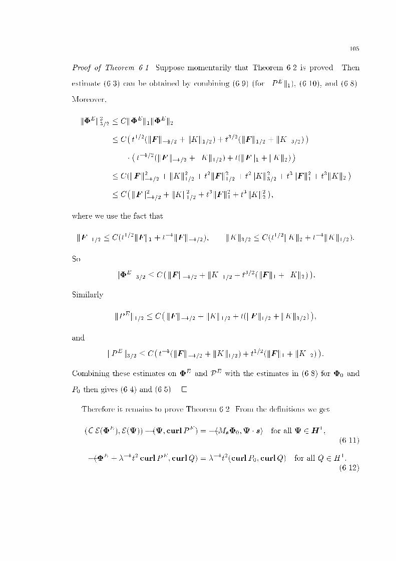
��
Proof of Theorem ���� Suppose momentarily that Theorem ��� is proved� Then
estimate ���� can be obtained by combining ���� for kPEk��� ����� and �����
Moreover�
k�Ek���� � Ck�Ek�k�Ek�
� C�t���kF k���� � kKk���� � t���kF k��� � kKk����
���t����kF k���� � kKk���� � tkF k� � kKk��
�� CkF k����� � kKk���� � t�kF k���� � t�kKk���� � t�kF k�� � t�kKk�
�� C
�kF k����� � kKk���� � t�kF k�� � t�kKk��
��
where we use the fact that
kF k��� � Ct���kF k� � t��kF k������ kKk��� � Ct���kKk� � t��kKk�����
So
k�Ek��� � C�kF k���� � kKk��� � t���kF k� � kKk��
��
Similarly
kPEk��� � C�kF k���� � kKk��� � tkF k��� � kKk����
��
and
kPEk��� � C�t��kF k���� � kKk���� � t���kF k� � kKk��
��
Combining these estimates on �E and PE with the estimates in ���� for �� and
P� then gives ���� and ����� �
Therefore it remains to prove Theorem ���� From the de�nitions we get
C E�E�� E ���� �� curlPE� � �hMs���� � si for all � �H�������
��E � ���t� curlPE� curlQ� � ���t�curl P�� curlQ� for all Q � H�������

��
We will prove Theorem ��� by choosing the appropriate test functions in these equa�
tions� First we need a lemma�
Lemma ��� Under the same conditions of Theorem ���� there is a constant C
such that for r � H����
jh�E � s� rij �Ct���krk���� � tkrk�����kF k� � kKk� � kPEk��
� Ct���krk����k�Ek��
Proof of Lemma ���� We de�ne the usual boundary��tted coordinates in a neigh�
borhood of the boundary� Let �� be a positive number less than the minimum radius
of curvature of �� and de�ne
�� � fz � �nzjz � ��� � � � �� g �
where nz is the outward unit normal to � at z� Let z�� � X��� Y ���� � � �� L��
be a parametrization of �� by arclength which we extend L�periodically to � � R�
The correspondence
�� �� � z � �nz � X�� � �Y ���� Y �� � �X ����
is a di�eomorphism of � ��� R�L on ��� For any function f � let #f �� �� denote
the change of variable to the �� ���coordinate�
Now� we de�ne an extension R of r to �� by
R�� �� � #r��e��t�
Then �nd a smooth cut�o� function � which is a function of � alone� independent of
� and t� and identically one for � � � ����� identically zero for � � ������ Thus
�R gives an extension to all of � and� by simple computations�
k�Rk� � Ct���krk����� k�Rk� � Ct����krk���� � t���krk������
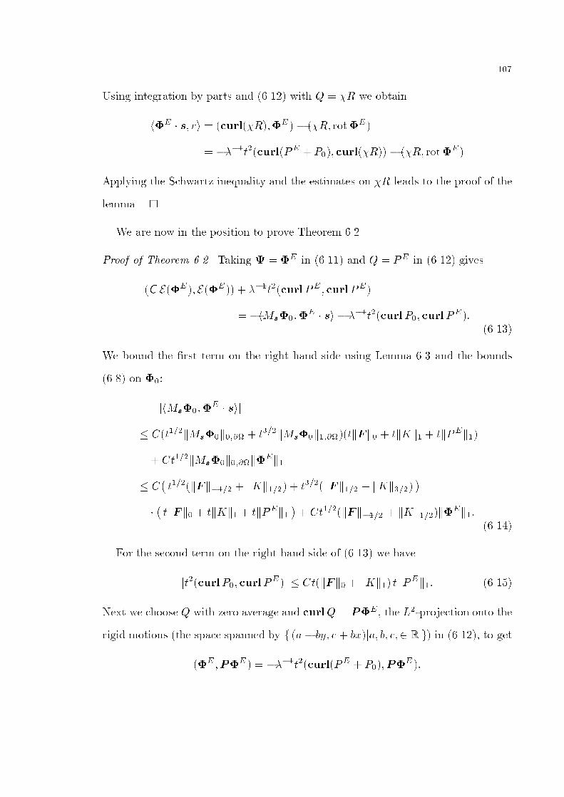
��
Using integration by parts and ����� with Q � �R we obtain
h�E � s� ri � curl�R���E � � �R� rot�E�
� ����t�curlPE � P��� curl�R�� � �R� rot�E�
Applying the Schwartz inequality and the estimates on �R leads to the proof of the
lemma� �
We are now in the position to prove Theorem ����
Proof of Theorem ���� Taking � � �E in ����� and Q � PE in ����� gives
C E�E�� E �E�� � ���t�curlPE � curlPE�
� �hMs����E � si � ���t�curl P�� curlP
E�������
We bound the �rst term on the right hand side using Lemma ��� and the bounds
���� on ���
jhMs����E � sij
� Ct���kMs��k���� � t���kMs��k�����tkF k� � tkKk� � tkPEk��
� Ct���kMs��k����k�Ek�
� C�t���kF k���� � kKk���� � t���kF k��� � kKk����
���tkF k� � tkKk� � tkPEk�
�� Ct���kF k���� � kKk����k�
Ek�������
For the second term on the right hand side of ����� we have
jt�curlP�� curlPE�j � CtkF k� � kKk�� tkP
Ek�� �����
Next we choose Q with zero average and curlQ � P�E � the L��projection onto the
rigid motions the space spanned by f a � by� c � bx�ja� b� c�� R g� in ������ to get
�E �P�E � � ����t�curlPE � P���P�E ��
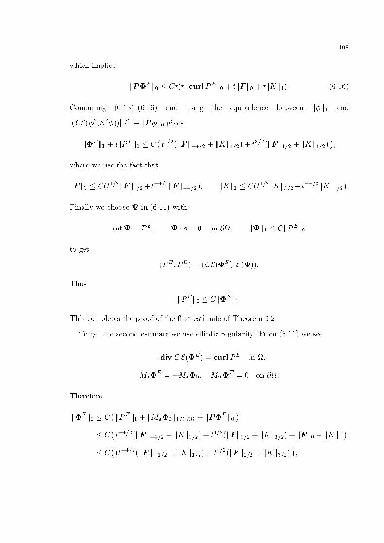
��
which implies
kP�Ek� � Cttk curlPEk� � tkF k� � tkKk��� �����
Combining ����� ����� and using the equivalence between k�k� and
jCE��� E ���j��� � kP�k� gives
k�Ek� � tkPEk� � C�t���kF k���� � kKk���� � t���kF k��� � kKk����
��
where we use the fact that
kF k� � Ct���kF k���� t����kF k������ kKk� � Ct���kKk���� t����kKk�����
Finally we choose � in ����� with
rot� � PE� � � s � on ��� k�k� � CkPEk�
to get
PE � PE� � CE�E�� E����
Thus
kPEk� � Ck�Ek��
This completes the proof of the �rst estimate of Theorem ����
To get the second estimate we use elliptic regularity� From ����� we see
�div C E�E� � curlPE in ��
Ms�E � �Ms��� Mn�
E � on ���
Therefore
k�Ek� � C�kPEk� � kMs��k������ � kP�Ek�
�� C
�t����kF k���� � kKk���� � t���kF k��� � kKk���� � kF k� � kKk�
�� C
�t����kF k���� � kKk���� � t���kF k��� � kKk����
��
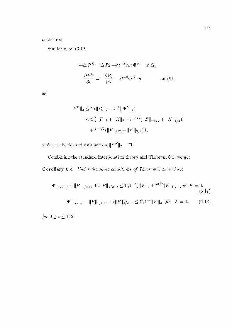
��
as desired�
Similarly� by �����
��PE � �P� � �t�� rot�E in ��
�PE
�n� �
�P��n
� �t���E � s on ���
so
kPEk� � CkP�k� � t��k�Ek��
� C�kF k� � kKk� � t����kF k���� � kKk����
� t����kF k��� � kKk������
which is the desired estimate on kPEk�� �
Combining the standard interpolation theory and Theorem ���� we get
Corollary ��� Under the same conditions of Theorem ���� we have
k�k����� � kPk����� � tkPk����� � C�t���kF k� � t���kF k�
�for K � �
�����
k�k����� � kPk����� � tkPk����� � C�t��kKk� for F � � �����
for � � � ����
��
References
�� R� A� Adams� Sobolev spaces� Academic Press� New York� ���� �� D� N� Arnold� F� Brezzi� and M� Fortin� A stable �nite element for the Stokes equa�
tions� Calcolo� �� ������� pp ������� �� D� N� Arnold and R� S� Falk� A uniformly accurate �nite element method for the
Reissner�Mindlin plate� SIAM J Num Anal � �� ������� pp �������� �� � The boundary layer for Reissner�Mindlin plate� SIAM J Math Anal� �� ������
pp ��� �� � The boundary layer for the Reissner�Mindlin plate model� soft simply supported�
soft clamped and free plates� to appear �� D� N� Arnold and X� Liu� Local error estimates for �nite element discretizations of the
Stokes equations� to appear �� D� N� Arnold� private communication �� D� N� Arnold and R� S� Falk� Edge E�ects in the Reissner�Mindlin Plate Theory�
Analytic and Computation Models of Shells� ���� �� I� Babu�ska and R� Rodr�iguez� The problem of the selection of an a�posteriori error
indicator based on smoothing techniques� Institute for Physical Science and Technology�BN����� �August �����
�� R� E� Bank and A� Weisser� Some a posteriori error estimators for elliptic partial
di�erential equations� Math Comp � �� ������� pp ������ ��� K� J� Bathe� Finite element procedure in engineering analysis� Prentice�Hall� ���� ��� J� H� Bramble and A� H� Schatz� Higher order local accuracy by local averaging in the
�nite element method� Math Comp � �� ������� pp ������ ��� F� Brezzi� On the existence� uniqueness� and approximation of saddle point problems
arising from Lagrangian multipliers � RAIRO Anal Numer � � ������� pp ������� ��� F� Brezzi� K� J� Bathe� and A� Fortin� Mixed�Interpolated elements for Reissner�
Mindlin plates� Int J Num Meth in Eng � �� ������� pp �������� ��� F� Brezzi and A� Fortin� Numerical approximation of Mindlin�Reissner plates� Math
Comp � �� ������� pp ������� ��� P� G� Ciarlet� The Finite Element Method for Elliptic Equations� North�Holland� Ams�
terdam � ����
��� � Finite element methods for elliptic boundary value problems� in Handbook of Nu�merical Analysis Volume II� P G Ciarlet and J L Lions� eds � Elsevier� Amsterdam�New York� ����
��� M� Crouzeix and P�A� Raviart� Conforming and non�conforming �nite element methods
for solving the stationary Stokes equations� RAIRO Anal Num�er � � R�� ������� pp �����
��� M� Dauge� Stationary Stokes and Navier�Stokes systems on two� or three�dimentional
domains with corners� Part I� Linearized equations� SIAM J Math Anal� � �������pp �����
�� J� Douglas� Jr� and F� A� Milner� Interior and superconvergence estimates for mixed
methods for second order elliptic problems� RAIRO Mod�el Math Anal Num�er � ��������� pp �������
��� J� Douglas� Jr� and J� E� Roberts� Global estimates for mixed methods for second order
elliptic problems� Math Comp � �� ������� pp ����� ��� R� Dur�an� M� A�M� Muschietti� and R� Rodr�iguez� On the asymptotic exactness of
error estimators for linear traingular �nite elements� Numer Math � �� ������� pp ������
��� R� Dur�an and R� Rodr�iguez� On the asymptotic exactness of Bank�Weisser�s estimator�Numer Math � �� ������� pp ������

���
��� E� Eriksson� Higher order local rate of convergence by mesh re�nement in the �nite ele�
ment method� Math Comp � �� ������� pp ������� ��� � Improved accurccy by adapted mesh re�nement in the �nte element method� Math
Comp � �� ������� pp ������ ��� E� Eriksson and C� Johnson� An Adaptive Finite Element Method for Linear Elliptic
Problems� Math Comp � � ������� pp ������� ��� � Adaptive �nite element methods for parabolic problems I� A linear model problem�
SIAM J Num Anal� �� ������� pp ����� ��� L� Gastaldi� Uniform interior error estimates for reissner�mindlin plate model� preprint ��� P� Grisvard� Probl�emes aux limits dans les polygones� Mode d�emploi � �� E D F Bulletin
de la direction des Etudes et Recherches S�erie C Math�ematiques� Informatiques� ���� �� T� R� Hughes� The �nite element method� Linear Static and Dynamic analysis� Prentice�
Hall� Englewood Cli�s� New Jersey� ���� ��� C� Johnson� in Numerical solutions of partial di�erential equations by the �nite element
method� CambridgeUniversity Press� NewYork�New Rochelle�Melbourne�Sydney� ����
��� J� L� Lions and E� Magnes� Nonhomogeneous boundary value problems and applications�Springer�Verlag� New York�Heidelberg�Berlin� ����
��� J� A� Nitsche and A� H� Schatz� Interior estimate for Ritz�Galerkin methods� Math Comp � �� ������� pp �������
��� A� H� Schatz� Lecture Notes in Mathematics � � Springer�Verlag� New York�Heidelberg�Berlin� ����
��� A� H� Schatz and L� B� Wahlbin� Interior Maximun norm estimates for �nite telement
methods� MATHC�� �� ������� pp ������� ��� � Maximun norm estimates in the �nite telement methods on plane polygonal do�
main� Part �� Math Comp � �� ������� pp ����� ��� � Maximun norm estimates in the �nite telement methods on plane polygonal do�
main� Part Re�nements� Math Comp � �� ������� pp ������� ��� � On the �nite element for singularly perturbed reaction�di�usion problems in two
and one dimensions� Math Comp � � ������� pp ����� ��� L� R� Scott and S� Zhang� Finite element interpolation of nonsmooth functions satisfying
bounday conditions� Math Comp � �� ������ pp ������� �� R� Temam� Navier�Stokes Equations� Amsterdam� Amsterdam� ���� ��� L� B� Wahlbin� Local Behavior in Finite Element Methods� in in Handbook of Numerical
Analysis Volume II� P G Ciarlet and J L Lions� eds � Elsevier� Amsterdam�NewYork�����
��� M� F� Wheeler and J� R� Whiteman� Superconvergence recovery of gradients on sub�
domains from piecewise linear �nite�elemen approximations� Numerical methods forpartial di�erential equations� � ������� pp �������
��� J� Xu� Theorey of Multilevel methods� Tech Report � ��� Department of Mathematics� thePenn State University� ����
��� C� Zhan and L� Wang� The interior Estimates for Nonconforming Finite elements� �� ��Chiness J Num Math � Appl � ���
��� J� Z� Zhu and O� C� Zienkiewicz� Adaptive techniques in the �nite element method�Comm in Appl Num methods� � ������� pp ������
��� O� C� Zienkiewicz and J� Z� Zhu� A simple error estimator and adaptive procedure for
practical engineering analysis� Internat J Numer Methods Engrg � �� ������� pp �������