intergenerational income mobility - an empirical ... · intergenerational income mobility - an...
TRANSCRIPT
Intergenerational Income Mobility -An Empirical Investigation for Austria
and the European Union∗
Wilfried Altzinger† Matthias Schnetzer‡
Vienna University of Economics and BusinessDepartment of Economics
October 2010 - Preliminary Version 1.4
This paper uses data from the European Union Statistics on Income andLiving Conditions (EU-SILC) 2005 to analyze intergenerational income mobil-ity in Austria compared to other European Union members. Applying variousmethodological approaches like least squares estimations or quantile regres-sions we reveal substantial differences in intergenerational mobility betweenScandinavian countries and Continental Europe. The results show that theperception of fast social advancement in Austria is limited.
JEL-Classification: E24, J62, D30Keywords: Intergenerational Income Mobility, Generational Mobility,
Income Distribution, Austria
∗The authors are grateful for useful comments and suggestions to Pirmin Fessler, Dieter Gstach, JohannesLedolter, Jesus Crespo-Cuaresma, Daniel Schnitzlein and Philippe van Kerm. Financial support fromthe Oesterreichische Nationalbank (OeNB) is gratefully acknowledged.
†E-Mail: [email protected]‡E-Mail: [email protected]
1
1. Introduction
There is a broad consensus in society as far as the perception of the rise from rags toriches is concerned. It is widely thought to be indisputable that certain individual effortalmost automatically leads to well-paid jobs. Haller (2005) shows that since the 1980sviews of a mobile society and economy is predominant in Austria. In 1986, 64 percentof Austrians agreed to the statement, that every hard working person has the chance toachieve social advancement. In 1993, 69 percent supported this opinion and in 2003 still 65agreed to this view1. It is therefore of great interest if, and furthermore to which extent,the social status of an individual is determined by the economic or social situation of theancestor. If it turns out that wages are independent between generations and income is notpredetermined by the parental economic status, this would support the above mentionedview.
From a sociologic as well as from an economic perspective limited social mobility impliesloss of efficiency, since children from socially disadvantaged families hardly have access tothe market of so-called high potentials even though they would have specialized skills.Resources would therefore not be deployed adequately which has social and political con-sequences. According to Bjorklund/Jantti (2009, p. 492), in the last centuries, the UnitedStates were conjectured to be a highly mobile society compared to Europe. While individ-ual income mobility was low, class solidarity and consequently left-wing political partiesand unions became stronger in Europe than in the United States.
There has been plenty of research on mobility, however there were considerable differ-ences in the methods used by economists and sociologists. For instance, while Pareto(1935) dealt with the circulation of the elite in his book ”The Mind and Society”, Becker/Tomes (1979) intended to create an integrative, consistent model of intergenerational mo-bility on the basis of utility maximization of households. Their work is known as a seminalcontribution for the explanation of the transmission of economic inequality across genera-tions. It has been used to analyze the distribution of income across families, across regionsor across countries2. Parents are said to derive utility on the one hand by own consump-tion and on the other hand by their child’s future well-being. The descendant’s realizedhuman capital is advanced by investment ,such as education or health care3 or endowmentsthat are transmitted across generations, i.e. genetic constitutions as well as endowmentsacquired by certain family cultures. However, the contribution of genetic factors is stillrather unclear and very controversial. Some authors, especially those familiar to sociologyor psychology, focused on this debate, famously entitled ”Nature versus Nurture”.
Zimmerman (1992) mentions in a few words and notes, that regression estimates arenot capable of capturing influences of cultural or genetic endowments. He refers to somearticles published in the 1970s and 1980s concerning the nature versus nurture debate ineconomic outcomes. However, for most scientists the discussion of nature and nurture asdichotomy is out of date4. The modern approach in the relevant literature is the calculation
1See Haller (2005, p. 57)2See Durlauf 1996 or Benabou 19943Such investments may be performed by parents or the public sector, which could be seen as perfect
substitutes (Bjorklund/Jantti 2009, p. 493).4”By now most scientists reject both the nineteenth-century doctrine that biology is destiny and the
2
of income elasticities between two generations as well as the probability of a movementalong the income distribution, which we will carry out in this article as well.
In Chapter 2 we provide a short literature survey. Although there is much emphasis puton mobility in the United States, we concentrate on literature based on European countries,since our main focus lies on the 27 European Union members. The bulk of articles dealswith data problems regarding the investigation of intergenerational mobility as well asdifficulties with cross-country analysis. This leads straightforward to our Chapter 3 ondata, where we describe the European Union Survey on Income and Living Conditions(EU-SILC) as well as issues concerning sample selection. In Section 4 we elaborate severalmethods for the analysis of intergenerational mobility such as income elasticities or quantileregression approaches. Moreover, we focus on the critique regarding these methods in therelevant literature. Finally we present the main results in Chapter 5.
2. Literature At A Glance
While the current state of research in countries like Austria or Germany is extremelyweak, there has been plenty of researchon an international scale. Mulligan (1999, p. 187)presents a detailed list of articles concerning intergenerational mobility across severaltopics (see Table 1). 16 articles among them deal with earnings or wages and estimateincome elasticities between 0.11 and 0.59 and an average value of 0.34. Solon (2002) liststwelve articles concerning intergenerational mobility in countries other than the UnitedStates. He refers to studies in Canada, Finland, Germany, Malaysia, South Africa, Swedenand the United Kingdom which calculate mobility between fathers and sons with elasticityvalues between 0.11 (Germany) and 0.57 (United Kingdom). Most of these elasticitycoefficients come from least square estimates of a log-linear regression with age controlsfor both generations.
Table 1: Studies of Intergenerational Mobility
Economic Characteristic Number of Estimates Range Average1. Years of schooling 8 .14-.45 .292. Log earnings or wages 16 .11-.59 .343. Log family income 10 .14-.65 .434. Log family wealth 9 .27-.76 .505. Log family consumption 2 .59-.77 .68
(Source: Mulligan 1999, p. 187)
For the case of Sweden, Osterberg (2000) analyses tax-data files with regard to intergen-erational transmissions of earnings status. Osterberg uses data from the Swedish IncomePanel (SWIP), which consists of a representative 1-percent-sample drawn from the regis-ter of total population (RTB). The information on income was gathered in two different,three years lasting periods from 1978 to 1980 for parents and from 1990 to 1992 for thechildren. This leads to varying mean ages for parents (fathers: 52, mothers: 49) and
twentieth-century doctrine that the mind is a blank slate”, Steven Pinker, Professor of Psychology atHarvard University wrote in an article.
3

children (37) at the point of observation. The author concentrates on regression resultsas well as on transition matrices with respect to gender and compares his results with thework of Bjorklund/Jantti (1997). Osterberg reports high intergenerational income mobil-ity in Sweden compared to estimations from most other countries. He derives correlationvalues varying between 0.11 and 0.18, depending on different restrictions. Solon (2002)cites a comparable study by Bjorn Gustafsson (1994) for Swedish father-son pairs with anelasticity value of 0.14, which is near Osterberg’s results.
Given the scarcity of data sources and the intricacy of the subject, the investigation ofintergenerational income mobility in Austria has been a rare field of research. Accordingto Statistics Austria, actually not a single analysis of intergenerational income mobility inAustria has been conducted yet5. To our knowledge there are only few articles on wagemobility within one generation in Austria like Hofer/Weber (2001) or Raferzeder/Winter-Ebmer (2004). Based on a special module in the EU-SILC 2005, some intergenerationalcalculations were finally carried out by Statistik Austria (2007a). The focus of the modulewas to reconstruct the former living conditions of adult participants. Various relevantvariables were requested, including the financial situation of the parental household and theeducational level as well as the occupational status of mothers and fathers. Fessler/Schurz(2009) analyze the intergenerational transmission of educational attainment in Austria.The authors state that compared to other European countries, the level of educationalmobility in Austria is similar to Italy or Slovenia and consequently lower than in theNetherlands, Finland or Sweden. In Chapter 5.1 we will see, how accurate this analysis isfor the case of intergenerational income mobility as well.
For Germany, Schnitzlein (2008) provides a collection of several studies on intergenera-tional income mobility carried out between 1997 and 2006. He presents an overview of theincome elasticity6 between fathers and sons. According to the referred authors, observedintergenerational mobility is higher in Germany than in the United States. However, thisis the result of very few studies and the findings should not be taken as irrevocable. Inmost common studies fathers and sons are the benchmark for the analysis of intergen-erational transmission of income, since in most countries females have significantly lowerlabor participation rates. According to Schnitzlein, recent studies published results forboth genders, however the amount of mobility studies relating to gender issues in Ger-many is diminutive. Schnitzlein shows estimates of intergenerational income elasticityvalues for Germany between 0.10 and 0.37, which means, that a marginal advance in thelogarithmic income of parents by one unit leads to an increase in the descendant’s logarith-mic income of 0.10 to 0.37 units. These positive regression coefficients may be interpretedas a positive relationship between earnings of fathers and sons, and hence limited incomemobility. Schnitzlein himself calculates coefficients of 0.172 for sons and 0.202 for daugh-ters. By the evaluation of transition matrices, Schnitzlein (2008) expects a high level ofintergenerational mobility in Germany.
5Statistik Austria (2007a, p. 61)6Most empirical analysis is based on a simple regression equation, denoted by
ln Yi,t = α+ β · ln Yi,s + εi,t
where ln Yi,t is the logarithmic life time income of a descendant of family i. This is determined bythe average income of his generation α, a noise term εi,t and the influence of the parental logarithmicincome of his parents ln Yi,s. The coefficient β measures the income elasticity between two generations(see Corak 2004, p. 10).
4
Zimmerman (1992) cites several studies for income elasticity in the United States. Thestudies revealed the elasticity coefficients of children’s earnings with respect to parent’searnings to be between 0.15 and 0.45. Zimmerman himself estimates the elasticity of de-scendant’s earnings with respect to parental income on 0.4. From a vast pool of studieson intergenerational income mobility, other relevant literature has been provided by Vo-gel (2006) and Schafer/Schmidt (2009) for Germany, Kopczuk/Saez/Song (2010) for theUnited States, Atkinson (1981) and Dearden/Machin/Reed (1997) for United Kingdom,Bjorklund/Jantti (1997) for Sweden as well as Corak/Heiz (1996) for the case of Canada,and OECD (2010) and Causa/Dantan/Johansson (2009) for European OECD countries.Extensive work on North America and Europe has been published in a volume edited byCorak (2004).
3. Data
3.1. Data specification
The most evident problem of data recording for the investigation of intergenerational in-come mobility is to measure incomes for two generations during two different time periods.Bjorklund/Jantti (1997), for instance, have to estimate intergenerational income correla-tions for independent fathers and sons, because income data for consecutive generationswere not available for Sweden. Their technique based on predictions of progenitors’ earn-ings given their education and occupational status7. The same procedure is applied byAndrews/Leigh (2009) due to the lack of data. The authors approximate hourly wagesby a regression on a vector of dummies for occupations and age. The earnings of fathersin a certain occupation is then predicted to be the same as those of a 40 year old manin this occupation. Schnitzlein (2008) points out as well, that there is no data existing,that contains long term (or at best life time) earnings for two interconnected generations.For this reason economists find a remedy in approximations via annual observation timeseries8.
In Austria, there are no official data sources which offer information on incomes forsequenced periods9. Even the most reliable data set for the analysis of wage-related in-come distribution, which is the Austrian Income Tax Data, does not provide any linksbetween ancestors and descendants. Consequently, the only practicable method to inves-tigate intergenerational income mobility is the usage of survey data that include questionsconcerning the financial situation of ancestors.
The European Statistics on Income and Living Conditions (EU-SILC) provides suchdata in its 2005 questionnaire and again in the 2011 panel wave. The EU-SILC is a surveycarried out in private households with its central focuses on income, employment, living,health and financial conditions. The population of the survey are households with at leastone household member aged at least 16. The EU-SILC questionnaire replaced the Euro-pean Community Household Panel (ECHP) which was conceived as a sole panel survey.
7Osterberg (2000, p. 422)8Problems and potential biases are discussed by Becker/Tomes (1986) or Zimmerman (1992).9Statistik Austria (2007a, p. 61)
5
Since the last panel wave of the ECHP in 2001, no data on income and living conditionswas collected on a European scale10. The EU-SILC project was started with a regulationof the European Parliament in June 2003, pursuing the objective of a standardized surveyfor comparable analysis of economic conditions in European households.
As far as the income level of parents is concerned, a respective question was askedwithin the survey, whether there were financial problems in the respondent’s householdwhen he/she was aged 12 to 16 (5 levels from most of the time to never). In some countries(e.g. in Austria) the equivalent question was, how the respondent would characterize thefinancial situation of the household aged 12 to 16 (5 levels from very good to very bad).Consequently, five categorical groups were requested which will be our approximationfor wealth and income status of parents, where a value of one means very bad financialconditions and five means very good income status.
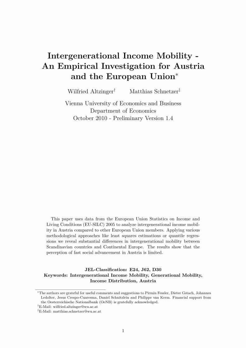
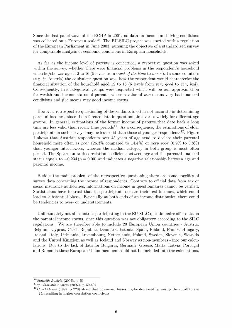
However, retrospective questioning of descendants is often not accurate in determiningparental incomes, since the reference date in questionnaires varies widely for different agegroups. In general, estimations of the former income of parents that date back a longtime are less valid than recent time periods11. As a consequence, the estimations of elderparticipants in such surveys may be less solid than those of younger respondents12. Figure1 shows that Austrian respondents over 45 years of age tend to declare their parentalhousehold more often as poor (26.3% compared to 14.4%) or very poor (6.9% to 3.8%)than younger interviewees, whereas the median category in both group is most oftenpicked. The Spearman rank correlation coefficient between age and the parental financialstatus equals to −0.234 (p = 0.00) and indicates a negative relationship between age andparental income.
Besides the main problem of the retrospective questioning there are some specifics ofsurvey data concerning the income of respondents. Contrary to official data from tax orsocial insurance authorities, informations on income in questionnaires cannot be verified.Statisticians have to trust that the participants declare their real incomes, which couldlead to substantial biases. Especially at both ends of an income distribution there couldbe tendencies to over- or understatements.
Unfortunately not all countries participating in the EU-SILC questionnaire offer data onthe parental income status, since this question was not obligatory according to the SILCregulations. We are therefore able to include 20 European Union countries - Austria,Belgium, Cyprus, Czech Republic, Denmark, Estonia, Spain, Finland, France, Hungary,Ireland, Italy, Lithuania, Luxembourg, Netherlands, Poland, Sweden, Slovenia, Slovakiaand the United Kingdom as well as Iceland and Norway as non-members - into our calcu-lations. Due to the lack of data for Bulgaria, Germany, Greece, Malta, Latvia, Portugaland Romania these European Union members could not be included into the calculations.
10Statistik Austria (2007b, p. 5)11cp. Statistik Austria (2007a, p. 59-60)12Couch/Dunn (1997, p. 220) show, that downward biases maybe decreased by raising the cutoff to age
25, resulting in higher correlation coefficients.
6
3.799
3.799
3.79914.34
14.34
14.3440.68
40.68
40.6834.45
34.45
34.456.738
6.738
6.7386.96
6.96
6.9626.24
26.24
26.2442.88
42.88
42.8819.36
19.36
19.364.56
4.56
4.560
0
010
10
1020
20
2030
30
3040
40
40very bad
very bad
very badbad
bad
badfair
fair
fairgood
good
goodvery good
very good
very goodvery bad
very bad
very badbad
bad
badfair
fair
fairgood
good
goodvery good
very good
very goodAge < 46
Age < 46
Age < 46Age > 45
Age > 45
Age > 45Percent
Perc
ent
PercentFinancial Situation of Parental Household
Financial Situation of Parental Household
Financial Situation of Parental Household
Figure 1: Parental Income for Age Groups in Austria
3.2. The EU-SILC 2005 income data
There are several variables on an individual’s income collected in the EU-SILC 200513.The reference period for the declaration of all income components was the calendar year2004, all income data was demanded on an annual or on a monthly basis. If respondentscould not or were not willing to reveal their exact income, they were asked to point ona certain level on an income range chart. The gross monthly income was categorizedinto 15 classes ranging from ”1-600” to ”8,001 and more” euros. For instance, 47 percentseized the possibility to declare their income out of investments (dividends, savings book,building loan contract, stocks and bonds, etc.) by the classification in categories. Thealternative to such charts would be an increasing probability of non-response and missingimportant information on income.
Several values were missing in the raw data. Missing net income values were imputedin EU-SILC, missing gross income values were computed using net-gross-conversion. Adetailed description of the imputation of income data into EU-SILC is given by StatistikAustria (2007b, p. 13). While in the EU-SILC 2004 survey approximately 20 percent ofemployee income were imputed, in 2005 this ratio could be reduced to 3 percent, especiallydue to some changes in the questionnaire14. Amongst other things, these changes led to anincrease of the disposable household income of about eight percent compared to EU-SILC2004, which is definitely not reflecting real income growth in Austria. A second reason forthis result is that households with lower income had a lower probability to continue theirparticipation in the longitudinal survey.
13For a detailed list see European Parliament (2003, p. 3).14see Statistik Austria (2007a, p. 77) and Statistik Austria (2007b, p. 25)
7
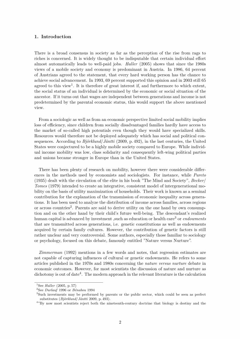
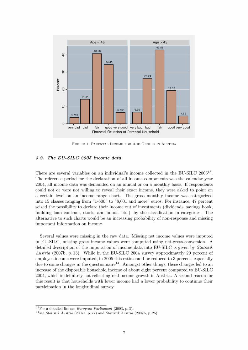
(a) Gender (b) Age
Figure 2: Mean Wage with Respect to Parental Income Class in Austria for Genderand Age
The dependent variable in this article are gross hourly wages of employed individuals15.Most respondents declare their work time per week, therefore the annualized wages couldbe calculated first on a weekly and furthermore on a hourly basis. These are based onwages and salaries paid in cash for time worked in main and any secondary job includingholiday pay and any additional payments during the year preceding the interview. Usinghours worked in the main job may lead to an over-estimation of wages for persons with twoor more jobs. Finally, the logarithmic hourly wages were derived. For those observationsfor which monthly wages in 2005 were available, we replaced the data from 2004 by thenewer ones. Osterberg (2000) refers to the problem of missing information on workinghours or wage per hour for Swedish data. The EU-SILC, however, is equipped with dataon working hours per week, hence we are able to correct for potential working time biases.In Figure 2 the (gross) mean hourly wages for all observations is presented for gender aswell as for age, given the particular parental income status from very poor (1) to very good(5). The mean wage is obviously increasing with the financial situation of the parentalhousehold. This is true for both characteristics, age and gender. Remarkably, the incomegaps between male and female as well as young and old respondents at both tails of thedistribution are significantly varying -especially with the second-best parental income rank(gender wage gap of 18% compared to 12% for the lowest income group).
3.3. Sample selection
In this paper, the emphasis is placed on the stability and robustness of the results. Theselection of the sample therefore is of decisive interest. Since the influence of parentaleconomic status on actual wages of descendants is the object of analysis, we concentrateon full time employees to obtain a homogeneous sample for our calculations. Self employed
15See Causa/Dantan/Johansson (2009, p. 10): ”This may potentially exaggerate the degree of intergener-ational wage mobility, to the extent that the offspring of higher-educated families are less likely to beinactive than the offspring of low-educated families.”
8
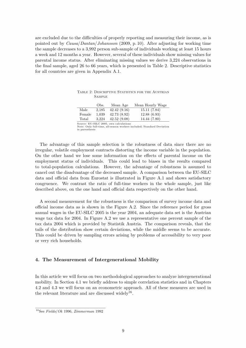
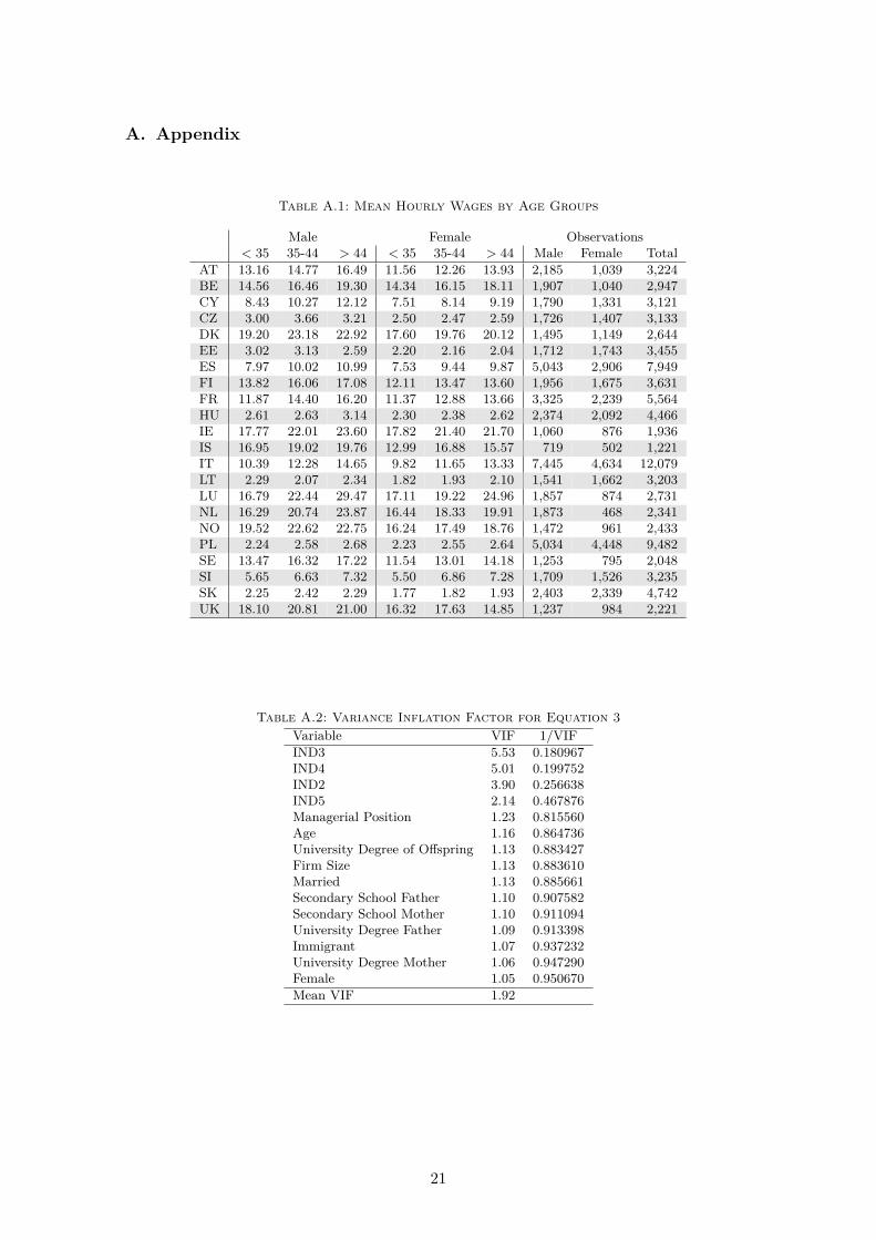
are excluded due to the difficulties of properly reporting and measuring their income, as ispointed out by Causa/Dantan/Johansson (2009, p. 10). After adjusting for working timethe sample decreases to a 3,992 person sub-sample of individuals working at least 15 hoursa week and 12 months a year. However, several of these individuals show missing values forparental income status. After eliminating missing values we derive 3,224 observations inthe final sample, aged 26 to 66 years, which is presented in Table 2. Descriptive statisticsfor all countries are given in Appendix A.1.
Table 2: Descriptive Statistics for the AustrianSample
Obs. Mean Age Mean Hourly WageMale 2,185 42.42 (9.16) 15.11 (7.84)Female 1,039 42.73 (8.92) 12.88 (6.93)Total 3,224 42.52 (9.08) 14.44 (7.80)
Source: EU-SILC 2005, own calculationsNote: Only full-time, all-season workers included; Standard Deviationin parenthesis
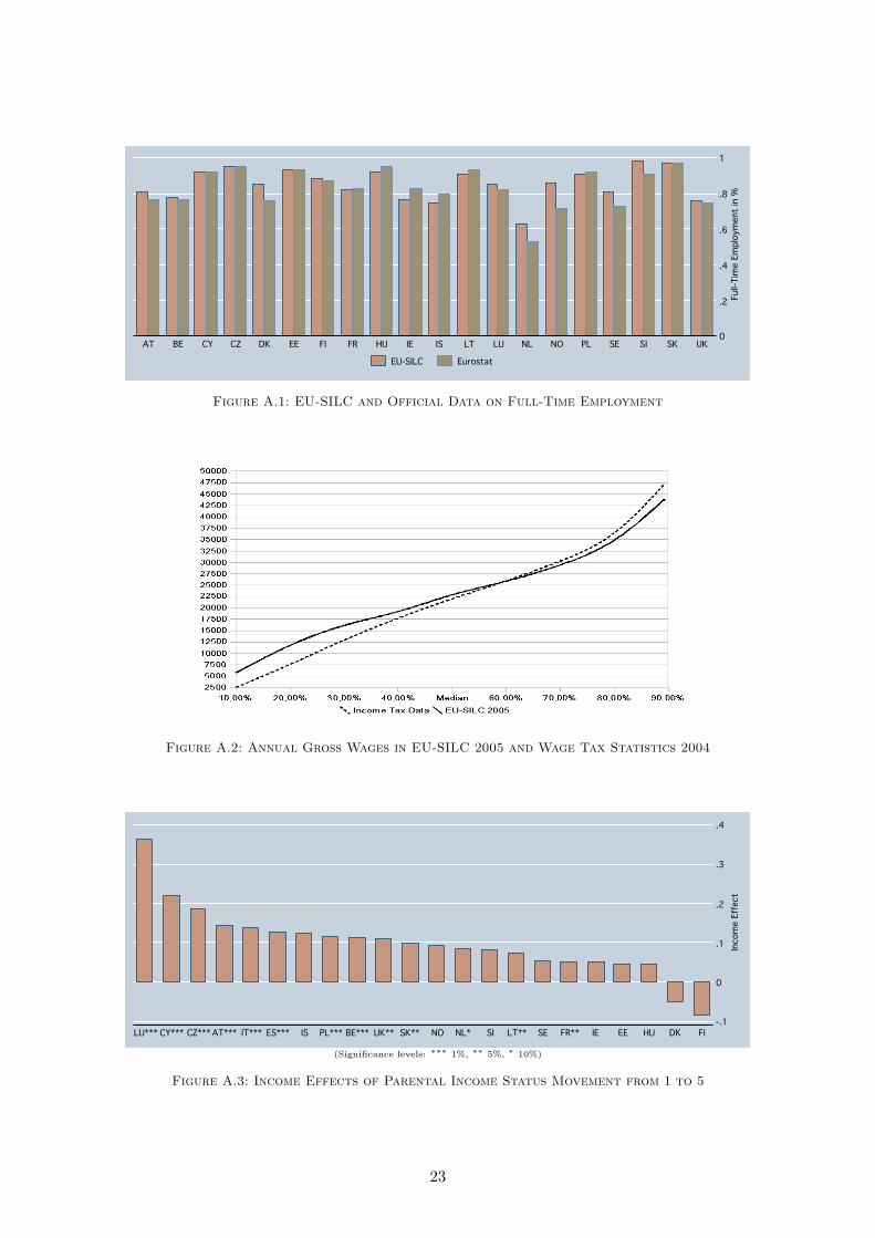
The advantage of this sample selection is the robustness of data since there are noirregular, volatile employment contracts distorting the income variable in the population.On the other hand we lose some information on the effects of parental income on theemployment status of individuals. This could lead to biases in the results comparedto total-population calculations. However, the advantage of robustness is assumed tocancel out the disadvantage of the decreased sample. A comparison between the EU-SILCdata and official data from Eurostat is illustrated in Figure A.1 and shows satisfactorycongruence. We contrast the ratio of full-time workers in the whole sample, just likedescribed above, on the one hand and official data respectively on the other hand.
A second measurement for the robustness is the comparison of survey income data andofficial income data as is shown in the Figure A.2. Since the reference period for grossannual wages in the EU-SILC 2005 is the year 2004, an adequate data set is the Austrianwage tax data for 2004. In Figure A.2 we use a representative one percent sample of thetax data 2004 which is provided by Statistik Austria. The comparison reveals, that thetails of the distribution show certain deviations, while the middle seems to be accurate.This could be driven by sampling errors arising by problems of accessibility to very pooror very rich households.
4. The Measurement of Intergenerational Mobility
In this article we will focus on two methodological approaches to analyze intergenerationalmobility. In Section 4.1 we briefly address to simple correlation statistics and in Chapters4.2 and 4.3 we will focus on an econometric approach. All of these measures are used inthe relevant literature and are discussed widely16.
16See Fields/Ok 1996, Zimmerman 1992
9
4.1. Spearman Correlation Coefficient
Since parental income in the EU-SILC 2005 is not provided as a floating variable but ratheras ranked proxy, the common Pearson correlation coefficient is not capable of measuringthe relationship between parental and offspring incomes. Instead we use the Spearmanrank correlation coefficient or better known as Spearman’s Rho, ranging between 1 and−1. A value of 1 indicates perfect positive relationship, while −1 means perfect negativerelationship. A score of 0 means no relation at all. The correlation coefficient is given by
ρ =∑i(xi − x)(yi − y)√∑
i(xi − x)2 ∑i(yi − y)2 ,
where xi and yi are the ranks. In our case, we are going to calculate the Spearman’s Rho forthe relationship between individuals earnings and parental income status. One particularproblem that arises with this approach is the loss of control for age. The correlationcoefficient is only able to capture the direct relationship between the two variables, butcan’t take into account that wages could rise with the age of an individual. This issue willbe handled with least squares regressions.
4.2. Critical Remarks on OLS methods
The common approach to intergenerational income transitions is the calculation of theregression coefficient β1 of the corresponding parental income to the income of descendants.Hence, the basic model yields
ln Yi,t = α+ β1 · ln Yi,s + εi,t (1)
where Yi,t is the logarithmic income of a descendant, Yi,s is the wage of the parents andεi is a white-noise error term. The coefficient β1 may be denoted as the intergenerationalincome elasticity17. Perfect mobility would be attained with a coefficient value of zero,whereas a value of one would report perfect immobility18. Values close to unity areindicative of limited mobility.
A cautious approach to the coefficients of the income variables is recommended byZimmerman (1992). According to him, there are potential life-cycle biases caused by thearbitrary date of observation of the sample. The most decisive problem is the particulartime of the data acquisition19. It is not possible to reveal whether a descendant, aged 20,draws a lower salary due to a low life-span income or due to the recent career entry. If thelatter is true, the person could certainly be in another position in the income distribution,17See Zimmerman (1992), Vogel (2006), Bjorklund/Jantti (2009), Schnitzlein (2008), etc.18An important constraint of this approach is given by Anderson/Leo (2009). The authors refer to the
implicit assumption that y and x are homogeneously linear across all socioeconomic strata. Otherwisethere could arise dangers with interpreting zero correlation with perfect mobility. ”Imagine a deter-ministic world (perfectly immobile) where below a certain parental income there is an exact negativerelationship between parent and child outcomes, whereas above that income there is an exact positiverelationship between parent and child outcomes; an appropriately balanced sample would yield 0 cor-relation with an inferred perfect mobility for what is a completely deterministic and immobile state.”(Anderson/Leo 2009, p. 621)
19Schnitzlein (2008, p. 12), Zimmerman (1992, p. 411)
10
if asked 15 years later. Ideally, income data would be available over the entire workinglives of parents and descendants respectively. Beyond these distortions, short-term proxiesfor lifetime economic status, such as annual earnings could be influenced by transitoryfluctuations. This measurement error could lead to a higher variance of the observed valuethan that of the underlying life-cycle value and consequently result in downward-biasedOLS-coefficients.
Another objection is mentioned by Corak (2004, p. 11). He argues that even small valuesfor β1 may indicate substantial income advantages for children, depending on the degreeof inequality in the parental earnings distribution. Corak therefore calculates the ratiobetween children from high income (H) and low income (L) backgrounds, raised to thepower of β and thus YH,t/YL,t = (YH,s/YL,s)β.
He gives an example with US-data reporting a earnings multiple of 12.0 for the topincome quintile compared to the bottom quintile. The ratio between high- and low-incomehouseholds would yield 12/1 and a elasticity coefficient β = 0.6 would result in (12/1)0.6.The intergenerational income elasticity then may be translated into an income advantagegiven a disproportionate income distribution of the parental generation, which is shown inTable 3. Hence, with an intergenerational elasticity of 0.6, children of high-income parentswill earn as much as 4.44 times the salaries of low-income parents (ceteris paribus andεi,t = 0).
Table 3: Income Elasticity and Income Advantage
β 0 0.2 0.4 0.6 0.8 1.0Income advantage 1.0 1.64 2.70 4.44 7.30 12.0
Source(Corak 2004, p. 12)
Bjorklund/Jantti (2009, p. 497) turn towards this issue as well. They argue, that theOLS-coefficient depends on income dispersion in two generations. Thus, if income inequal-ity rises from one to another generation, a larger coefficient will be needed to account forthe increased income variation in the second generation. Consequently, a elasticity co-efficient multiplied by the ratio of the standard deviations of parental and descendantincome should be preferred, ϕ = β(σf/σs). This correlation coefficient provides informa-tion how many standard deviations the child’s wage would change with a modification inthe standard deviation of the parental income.
O’Neill/Sweetman/Van de Gaer (2007, p. 160) focus on measurement errors in leastsquares estimations: ”Omitted variable bias, on the other hand, occurs when unobservedcharacteristics that are inherited from parents, such as ability, are also correlated withearnings. The OLS estimator mistakenly attributes the variation in earnings due to inher-ited endowments directly to parental earnings, leading us to overestimate the causal effectof parental earnings on children’s earnings. While the simple linear regression model pro-vides a useful summary of the conditional mean function, it is only a partial description ofthe joint distribution of earnings. When considering intergenerational mobility patternsthroughout the distribution, researchers have traditionally moved away from regressionbased models and relied instead upon transition matrices.” The briefly discussed issues on
11
least squares regressions lead to three established variants for measuring intergenerationalmobility - OLS, Spearman rank correlation coefficients and transition matrices.
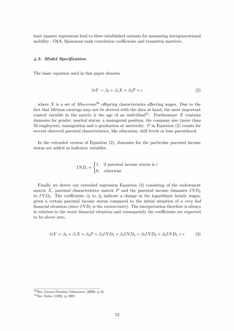
4.3. Model Specification
The basic equation used in this paper denotes
lnY = β0 + β1X + β2P + ε (2)
where X is a set of Mincerian20 offspring characteristics affecting wages. Due to thefact that lifetime earnings may not be derived with the data at hand, the most importantcontrol variable in the matrix is the age of an individual21. Furthermore X containsdummies for gender, marital status, a managerial position, the company size (more than50 employees), immigration and a graduation at university. P in Equation (2) counts forseveral observed parental characteristics, like education, skill levels or lone parenthood.
In the extended version of Equation (2), dummies for the particular parental incomestatus are added as indicator variables.
INDi ={
1, if parental income status is i0, otherwise
Finally we derive our extended regression Equation (3) consisting of the endowmentmatrix X, parental characteristics matrix P and the parental income dummies IND2to IND5. The coefficients β3 to β6 indicate a change in the logarithmic hourly wages,given a certain parental income status compared to the initial situation of a very badfinancial situation (since IND1 is the nummeraire). The interpretation therefore is alwaysin relation to the worst financial situation and consequently the coefficients are expectedto be above zero.
lnY = β0 + β1X + β2P + β3IND2 + β4IND3 + β5IND4 + β6IND5 + ε (3)
20See Causa/Dantan/Johansson (2009, p. 8)21See Solon (1992, p. 399)
12
5. Results
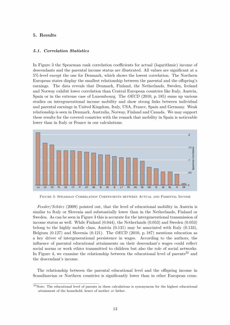
5.1. Correlation Statistics
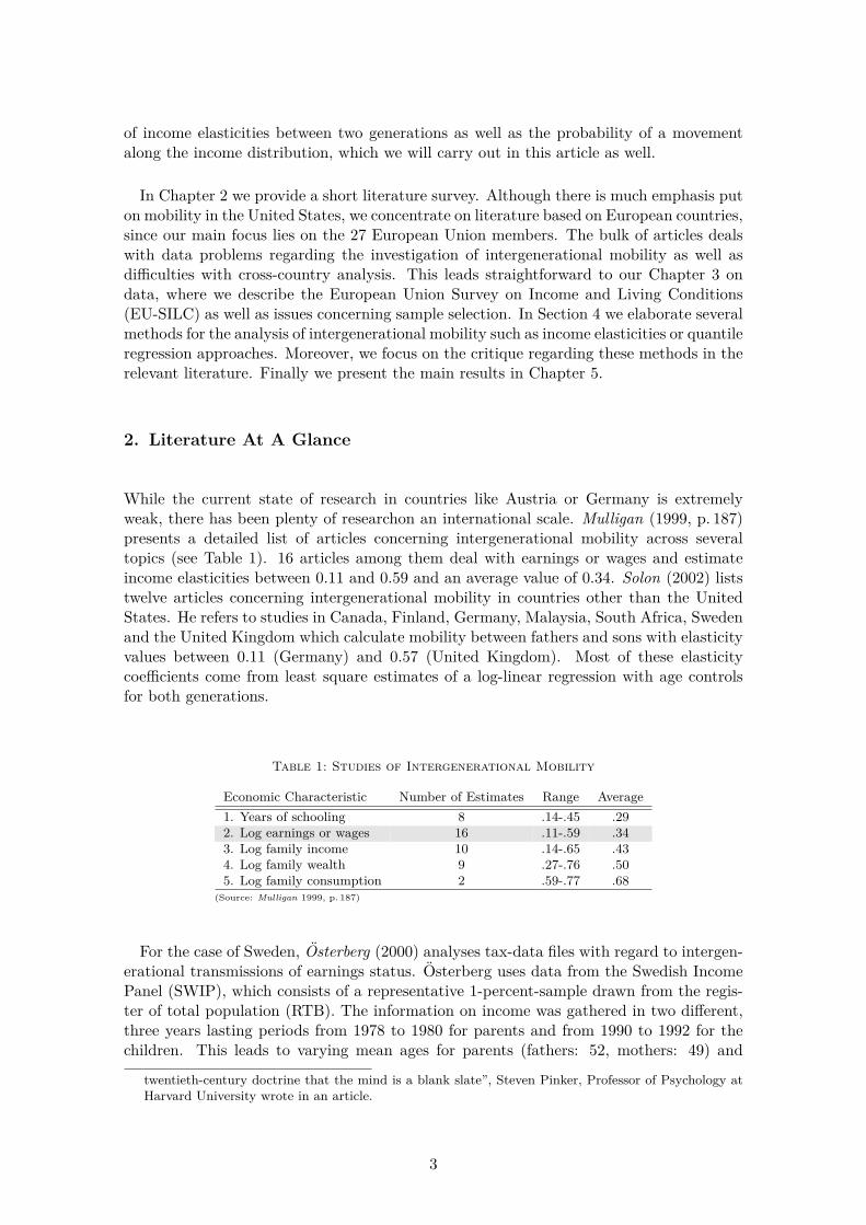
In Figure 3 the Spearman rank correlation coefficients for actual (logarithmic) income ofdescendants and the parental income status are illustrated. All values are significant at a5%-level except the one for Denmark, which shows the lowest correlation. The NorthernEuropean states display the smallest relationship between the parental and the offspring’searnings. The data reveals that Denmark, Finland, the Netherlands, Sweden, Icelandand Norway exhibit lower correlation than Central European countries like Italy, Austria,Spain or in the extreme case of Luxembourg. The OECD (2010, p. 185) sums up variousstudies on intergenerational income mobility and show strong links between individualand parental earnings in United Kingdom, Italy, USA, France, Spain and Germany. Weakrelationship is seen in Denmark, Australia, Norway, Finland and Canada. We may supportthese results for the covered countries with the remark that mobility in Spain is noticeablelower than in Italy or France in our calculations.0
0
0.05
.05
.05.1
.1
.1.15
.15
.15.2
.2
.2Spearman Correlation
Spea
rman
Cor
rela
tion
Spearman CorrelationLU
LU
LUCZ
CZ
CZES
ES
ESPL
PL
PLEE
EE
EECY
CY
CYIT
IT
ITAT
AT
ATBE
BE
BESI
SI
SIUK
UK
UKIE
IE
IELT
LT
LTFR
FR
FRHU
HU
HUSK
SK
SKNO
NO
NOIS
IS
ISSE
SE
SENL
NL
NLFI
FI
FIDK
DK
DK
Figure 3: Spearman Correlation Coefficients between Actual and Parental Income
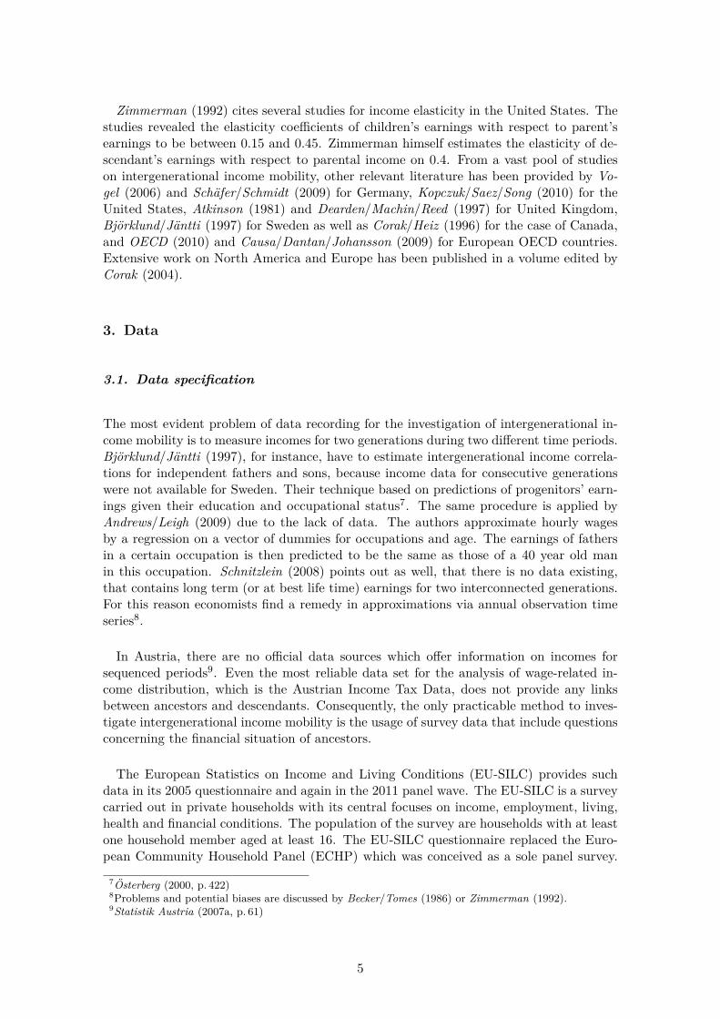
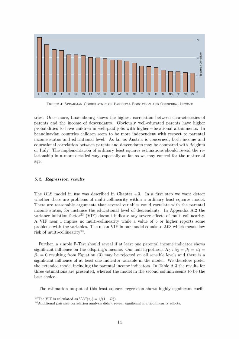
Fessler/Schurz (2009) pointed out, that the level of educational mobility in Austria issimilar to Italy or Slovenia and substantially lower than in the Netherlands, Finland orSweden. As can be seen in Figure 3 this is accurate for the intergenerational transmission ofincome status as well. While Finland (0.044), the Netherlands (0.053) and Sweden (0.053)belong to the highly mobile class, Austria (0.131) may be associated with Italy (0.133),Belgium (0.127) and Slovenia (0.121). The OECD (2010, p. 187) mentions education asa key driver of intergenerational persistence in wages. According to the authors, theinfluence of parental educational attainments on their descendant’s wages could reflectsocial norms or work ethics transmitted to children but also the role of social networks.In Figure 4, we examine the relationship between the educational level of parents22 andthe descendant’s income.
The relationship between the parental educational level and the offspring income inScandinavian or Northern countries is significantly lower than in other European coun-
22Note: The educational level of parents in these calculations is synonymous for the highest educationalattainment of the household, hence of mother or father.
13
0
0
0.1
.1
.1.2
.2
.2.3
.3
.3Spearman Correlation
Spea
rman
Cor
rela
tion
Spearman CorrelationLU
LU
LUEE
EE
EEHU
HU
HUIE
IE
IESI
SI
SIUK
UK
UKES
ES
ESLT
LT
LTCZ
CZ
CZSK
SK
SKBE
BE
BEAT
AT
ATPL
PL
PLFR
FR
FRIT
IT
ITIS
IS
ISFI
FI
FINL
NL
NLNO
NO
NOSE
SE
SEDK
DK
DKCY
CY
CY
Figure 4: Spearman Correlation of Parental Education and Offspring Income
tries. Once more, Luxembourg shows the highest correlation between characteristics ofparents and the income of descendants. Obviously well-educated parents have higherprobabilities to have children in well-paid jobs with higher educational attainments. InScandinavian countries children seem to be more independent with respect to parentalincome status and educational level. As far as Austria is concerned, both income andeducational correlation between parents and descendants may be compared with Belgiumor Italy. The implementation of ordinary least squares estimations should reveal the re-lationship in a more detailed way, especially as far as we may control for the matter ofage.
5.2. Regression results
The OLS model in use was described in Chapter 4.3. In a first step we want detectwhether there are problems of multi-collinearity within a ordinary least squares model.There are reasonable arguments that several variables could correlate with the parentalincome status, for instance the educational level of descendants. In Appendix A.2 thevariance inflation factor23 (VIF) doesn’t indicate any severe effects of multi-collinearity.A VIF near 1 implies no multi-collinearity while a value of 5 or higher reports someproblems with the variables. The mean VIF in our model equals to 2.03 which means lowrisk of multi-collinearity24.
Further, a simple F-Test should reveal if at least one parental income indicator showssignificant influence on the offspring’s income. Our null hypothesis H0 : β2 = β3 = β4 =β5 = 0 resulting from Equation (3) may be rejected on all sensible levels and there is asignificant influence of at least one indicator variable in the model. We therefore preferthe extended model including the parental income indicators. In Table A.3 the results forthree estimations are presented, whereof the model in the second column seems to be thebest choice.
The estimation output of this least squares regression shows highly significant coeffi-
23The VIF is calculated as V IF (xj) = 1/(1−R2j ).
24Additional pairwise correlation analysis didn’t reveal significant multicollinearity effects.
14
cients for nearly all explanatory variables. While gender and immigration have a negativeimpact on earnings, a leading position in the company and the possession of a universitydegree have a strong positive effect on income. Among the parental income status indi-cator variables, one is insignificant, one is significant on a 10%-level and two dummieson a 1%-level. One may conclude that there is no significant income difference betweendescendants, which declare their childhood household either very poor or poor. However,offsprings with good or very good financial background earn significantly more than theirvery poor peers.
This is a strong indicator that parental income does have an influence and intergenera-tional mobility is limited.
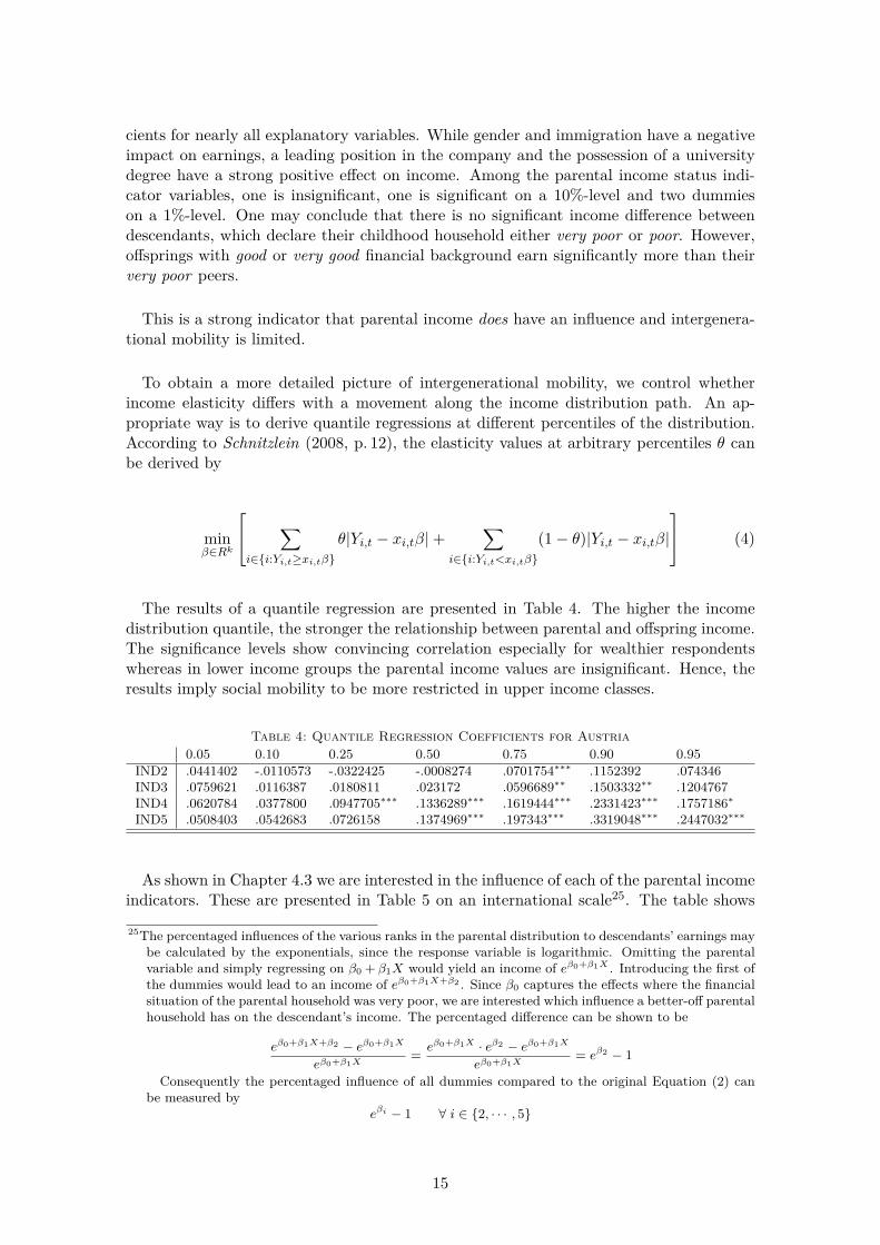
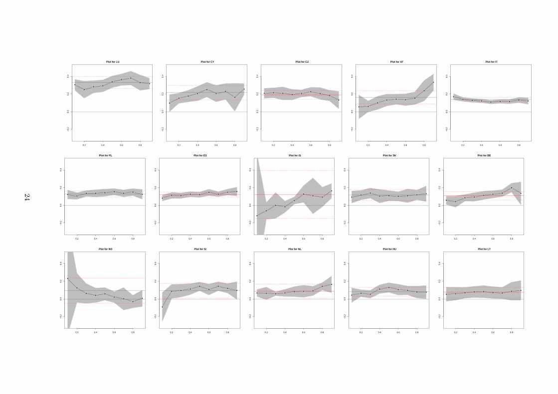
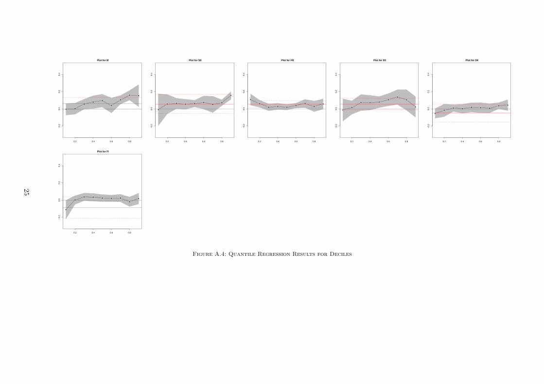
To obtain a more detailed picture of intergenerational mobility, we control whetherincome elasticity differs with a movement along the income distribution path. An ap-propriate way is to derive quantile regressions at different percentiles of the distribution.According to Schnitzlein (2008, p. 12), the elasticity values at arbitrary percentiles θ canbe derived by
minβ∈Rk
∑i∈{i:Yi,t≥xi,tβ}
θ|Yi,t − xi,tβ|+∑
i∈{i:Yi,t<xi,tβ}(1− θ)|Yi,t − xi,tβ|
(4)
The results of a quantile regression are presented in Table 4. The higher the incomedistribution quantile, the stronger the relationship between parental and offspring income.The significance levels show convincing correlation especially for wealthier respondentswhereas in lower income groups the parental income values are insignificant. Hence, theresults imply social mobility to be more restricted in upper income classes.
Table 4: Quantile Regression Coefficients for Austria0.05 0.10 0.25 0.50 0.75 0.90 0.95
IND2 .0441402 -.0110573 -.0322425 -.0008274 .0701754∗∗∗ .1152392 .074346IND3 .0759621 .0116387 .0180811 .023172 .0596689∗∗ .1503332∗∗ .1204767IND4 .0620784 .0377800 .0947705∗∗∗ .1336289∗∗∗ .1619444∗∗∗ .2331423∗∗∗ .1757186∗IND5 .0508403 .0542683 .0726158 .1374969∗∗∗ .197343∗∗∗ .3319048∗∗∗ .2447032∗∗∗
As shown in Chapter 4.3 we are interested in the influence of each of the parental incomeindicators. These are presented in Table 5 on an international scale25. The table shows
25The percentaged influences of the various ranks in the parental distribution to descendants’ earnings maybe calculated by the exponentials, since the response variable is logarithmic. Omitting the parentalvariable and simply regressing on β0 + β1X would yield an income of eβ0+β1X . Introducing the first ofthe dummies would lead to an income of eβ0+β1X+β2 . Since β0 captures the effects where the financialsituation of the parental household was very poor, we are interested which influence a better-off parentalhousehold has on the descendant’s income. The percentaged difference can be shown to be
eβ0+β1X+β2 − eβ0+β1X
eβ0+β1X= eβ0+β1X · eβ2 − eβ0+β1X
eβ0+β1X= eβ2 − 1
Consequently the percentaged influence of all dummies compared to the original Equation (2) canbe measured by
eβi − 1 ∀ i ∈ {2, · · · , 5}
15

the income effects of a movement in the parental income situation based on the initialsituation to be very poor. The last column therefore shows the increase of wages if parentsare very rich compared to the lowest income level. Significant and high values imply thatthere is an influence of parental income status and hence limited social mobility. As far asNordic countries like Sweden, Norway, Denmark or Finland are concerned, the regressioncoefficients are entirely senseless. Not a single one is significant on sensible levels, whichimplies that links between parental and offspring income can not be verified. The incomeeffects of a parental income status movement from the lowest to the highest class on thedescendant’s earnings are seen as the best indicator, how mobile a wage structure is. Avalue of zero would again mean no influence of the family background, the higher the valuethe lower the intergenerational mobility.
Table 5: Income Effects on Parent Status Movement
1→ 2 1→ 3 1→ 4 1→ 5LU .2054∗∗∗ .2639∗∗∗ .3295∗∗∗ .3633∗∗∗CY .0743∗ .15∗∗∗ .1753∗∗∗ .2185∗∗∗CZ .0743∗∗ .1138∗∗∗ .1681∗∗∗ .1866∗∗∗AT .0451 .0598∗ .1429∗∗∗ .1444∗∗∗IT .0477∗∗∗ .1096∗∗∗ .1235∗∗∗ .1386∗∗∗ES .0065 .0644∗∗∗ .0682∗∗∗ .1248∗∗∗IS .2398 .1598 .1211 .1236PL .0412 .0889∗∗∗ .0659∗∗∗ .1141∗∗∗BE .0359 .094∗∗∗ .0736∗∗ .1113∗∗∗UK -.0492 .0992∗ .0322 .109∗∗SK .0385 .0334 .054 .0976∗∗NO .1753 .0627 .0868 .0915NL .1099∗ .0725 .0465 .085∗SI .0263 .0528 .0017 .082LT .0107 .0221 .0466 .073∗∗SE .0121 -.005 .0044 .0545FR -.0284 .0399 .0458∗ .0516∗∗IE -.062 .007 .0598 .0511EE .0013 .0706∗ .075∗2 .0448HU -.0046 .0121 .0218 .0441DK -.0533 -.0254 -.0121 -.0528FI .0832 -.0442 -.0465 -.0836
The results are illustrated in Figure A.3. While Scandinavian countries seem to featuremobile social structures, Southern European countries as well as Luxembourg show limitedmobility. Austria is ranked behind Luxembourg, Cyprus and Czech Republic as one ofthe lowest mobile countries, followed by Italy, Poland and Spain.
Andrews/Leigh (2009) investigate the relationship between inequality and intergenera-tional mobility. By proxying father’s earnings via occupational data, they reveal that sonswho grew up in countries that were more unequal in the 1970s were less likely to haveexperienced social mobility by the late 1990s26. Recent research by the OECD (2010,p. 193) confirms that higher inequality is associated with lower intergenerational mobil-ity. According to the authors a higher income dispersion could lead to higher returnsto education and individuals whose investments to education are not limited by familybackground may benefit in particular. Comparing the results in Figure 5 with the figures
26The authors use Gini coefficients from the Luxembourg Income Study (LIS).
16
in Andrews/Leigh (2009) and OECD (2010), the previous findings may be supported.
●●
●
●
●
●
●
●
●●
●
●
●
●
●
●
●
●
●
●
●
●
0.25 0.30 0.35
0.00
0.05
0.10
0.15
0.20
Gini Coefficient
Cor
rela
tion
Coe
ffici
ent
ATBE
CY
CZ
DK
EE
ES
FI
FRHUIE
IS
IT
LT
LU
NL
NO
PL
SE
SI
SK
UK
(a) All Countries (R2 = 0.23)
●●
●
●
●
●
●
●
●
●
●
●
●
0.25 0.30 0.35
0.00
0.05
0.10
0.15
0.20
Gini Coefficient
Cor
rela
tion
Coe
ffici
ent
ATBE
DK
ES
FI
FRIE
IS
IT
NL
NO
SE
UK
(b) Western ex LU (R2 = 0.66)
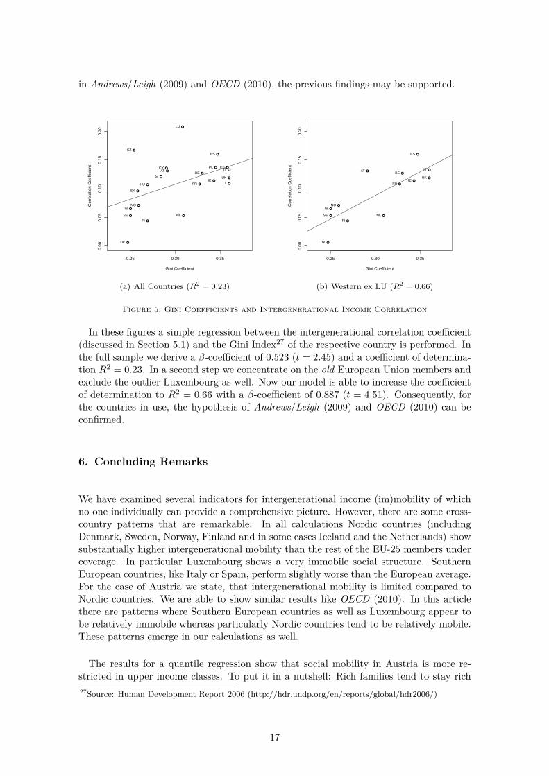
Figure 5: Gini Coefficients and Intergenerational Income Correlation
In these figures a simple regression between the intergenerational correlation coefficient(discussed in Section 5.1) and the Gini Index27 of the respective country is performed. Inthe full sample we derive a β-coefficient of 0.523 (t = 2.45) and a coefficient of determina-tion R2 = 0.23. In a second step we concentrate on the old European Union members andexclude the outlier Luxembourg as well. Now our model is able to increase the coefficientof determination to R2 = 0.66 with a β-coefficient of 0.887 (t = 4.51). Consequently, forthe countries in use, the hypothesis of Andrews/Leigh (2009) and OECD (2010) can beconfirmed.
6. Concluding Remarks
We have examined several indicators for intergenerational income (im)mobility of whichno one individually can provide a comprehensive picture. However, there are some cross-country patterns that are remarkable. In all calculations Nordic countries (includingDenmark, Sweden, Norway, Finland and in some cases Iceland and the Netherlands) showsubstantially higher intergenerational mobility than the rest of the EU-25 members undercoverage. In particular Luxembourg shows a very immobile social structure. SouthernEuropean countries, like Italy or Spain, perform slightly worse than the European average.For the case of Austria we state, that intergenerational mobility is limited compared toNordic countries. We are able to show similar results like OECD (2010). In this articlethere are patterns where Southern European countries as well as Luxembourg appear tobe relatively immobile whereas particularly Nordic countries tend to be relatively mobile.These patterns emerge in our calculations as well.
The results for a quantile regression show that social mobility in Austria is more re-stricted in upper income classes. To put it in a nutshell: Rich families tend to stay rich27Source: Human Development Report 2006 (http://hdr.undp.org/en/reports/global/hdr2006/)
17
or like Pareto (1935) formulated: It’s a circulation of elites. Moreover we state, that in-equality and immobility are linked together. The higher the inequality in a country, thelower the mobility and consequently the chances for social advancement. Again, Nordiccountries are amongst the most equal and mobile structures. Policies for higher socialmobility should therefore be accompanied by policies for more equal societies. Accordingto OECD (2010, p. 194) progressive tax systems and social transfer programs should notonly help to make a society more equal but also strengthen the chances for individualsocial and economic advancement.
For a decisive part individual positioning in social systems results from origin and edu-cation status. In this context, education systems are widely discussed. There are variousvariables taking effect on the degree of social mobility. While study grants (Studienbei-hilfe) may have a positive effect on social mobility, since students from poor families arefinancially backed, the rigid educational system in Austria prevents indigent individualsto get to university. Consequently, not only tax policy or social welfare may account forintergenerational mobility but also basic modifications of the educational system are de-cisive. Apparently, Scandinavian countries could be a model worth studying in the rest ofEurope.
References
Anderson, Gordon/Leo, Teng Wah (2009): Child Poverty, Investment in Children and GenerationalMobility: The Short and Long Term Wellbeing of Children in Urban China after the OneChild Policy. Review of Income and Wealth, 55, Issue 0, pp. 607–629
Andrews, Dan/Leigh, Andrew (2009): More inequality, less social mobility. Applied EconomicsLetters, 16, Issue 15, pp. 1489 – 1492
Atkinson, A.B. (1981): On Intergenerational Income Mobility in Britain. Journal of Post-KeynesianEconomics, 3, No. 2, pp. 184–217
Atkinson, A.B./Bourguignon, F./Morrisson, C. (1992): Empirical Studies of Earnings Mobility.Harwood Academic Publishers, Chur, Switzerland
Becker, Gary/Tomes, Nigel (1979): An Equilibrium Theory of the Distribution of Income andIntergenerational Mobility. The Journal of Political Economy, Vol. 87, No. 6, pp. 1153–1189
Becker, Gary/Tomes, Nigel (1986): Human Capital and the Rise and Fall of Families. Journal ofLabor Economics, 4, No. 3, pp. S1–S39
Benabou, Roland (1994): Human Capital, Inequality, and Growth: A Local Perspective. EuropeanEconomic Review, Vol. 38, pp. 817–826
Bjorklund, Anders/Jantti, Markus (1997): Intergenerational Income Mobility in Sweden comparedto the United States. American Economic Review, 87, No. 5, pp. 1009–1018
Bjorklund, Anders/Jantti, Markus (2009): Intergenerational Income Mobility and the Role ofFamily Background. In: Salverda, Wiemer: The Oxford handbook of economic inequality.Oxford University Press, pp. 491–521
Bowles, Samuel/Gintis, Herbert/Groves, Melissa Osborne (2008): Introduction to UnequalChances: Family Background and Economic Success. In: Unequal Chances: Family Back-ground and Economic Success. Princeton University Press
Burkhauser, Richard V./Couch, Kenneth A. (2009): Intragenerational Inequality and Intertempo-ral Mobility. In: Salverda, Wiemer: The Oxford handbook of economic inequality. OxfordUniversity Press, pp. 522–545
Causa, Orsetta/Dantan, Sophie/Johansson, Asa (2009): Intergenerational Social Mobility in Eu-ropean OECD Countries. OECD Economics Department Working Papers No. 709
18
Corak, M./Heiz, A. (1996): The Intergenerational Income Mobility of Canadian Men. AnalyticalStudies Branch Research Paper Series 89
Corak, Miles (2004): Generational Income Mobility in North America and Europe. CambridgeUniversity Press
Couch, Kenneth A./Dunn, Thomas A. (1997): Intergenerational Correlations in Labor MarketStatus: A Comparison of the United States and Germany. The Journal of Human Resources,32, No. 1, pp. 210–232
Dearden, L./Machin, S./Reed, H. (1997): Intergenerational Mobility in Britain. The EconomicJournal, 107, pp. 47–66
Durlauf, Steven (1996): A Theory of Persistent Income Inequality. Journal of Economic Growth,Vol. 1, No. 1, pp. 75–93
European Parliament (2003): Regulation (EC) No 1980/2003. Official Journal of the EuropeanUnion Volume 46, L298
Fessler, Pirmin/Schurz, Martin (2009): Intergenerational Transmission of Educational Attainmentin Austria. IAFFE Conference in Boston, June 2009
Fields, Gary S./Ok, Efe A. (1996): The Measurement of Income Mobility: An Introduction tothe Literature. C.V. Starr Center for Applied Economics, New York University – WorkingPapers 96-05
Forster, Michael (2008): Einkommensverteilung und Armut im OECD-Raum. In: Proceedings ofOeNB Workshops. Volume No. 16, OeNB
Geweke, John/Marshall, Robert C./Zarkin, Gary A. (1986): Mobility Indices in Continuous TimeMarkoc Chains. Econometrica, Vol. 54, No. 6, pp. 1407–1423
Haller, Max (2005): Auf dem Weg zur mundigen Gesellschaft? Wertwandel in Osterreich 1986bis 2003. In: Schulz, Wolfgang/Haller, Max/Grausgruber, Alfred: Osterreich zur Jahrhun-dertwende. Gesellschaftliche Werthaltungen und Lebensqualitat 1986-2004. VS Verlag furSozialwissenschaften, Wiesbaden, pp. 33–73
Hofer, Helmut/Weber, Andrea (2001): Wage Mobility in Austria 1986-1996. Institute for AdvancedStudies, Vienna Economics Series 108
Kopczuk, Wojciech/Saez, Emmanuel/Song, Jae (2010): Earnings Inequality and Mobility in theUnited States: Evidence from Social Security Data since 1937. Quarterly Journal of Eco-nomics, 125, No. 1, pp. 91–128
Mulligan, Casey (1999): Galton versus the Human Capital Approach to Inheritance. The Journalof Political Economy, Vol. 107, No. 6, pp. 184–224
OECD (2010): Economic Policy Reforms - Going for Growth 2010.Oesterreichische Nationalbank (2008): Dimensions of Inequality in the EU., No. 16O’Neill, Donal/Sweetman, Olive/Van de Gaer, Dirk (2007): The effects of measurement error
and omitted variables when using transition matrices to measure intergenerational mobility.Journal of Economic Inequality, 5, No. 2, pp. 159–178
Osterberg, Torun (2000): Intergenerational Income Mobility in Sweden: What do Tax-Data show?Review of Income and Wealth, 46, Issue 4, pp. 421–436
Pareto, Vilfredo (1935): Mind and Society [Trattato Di Sociologia Generale], Harcourt, Brace.Prais, S.J. (1955): Measuring Social Mobility. Journal of the Royal Statistical Society, Series A,
No. 118, pp. 56–66Raferzeder, Thomas/Winter-Ebmer, Rudolf (2004): Who is on the Rise in Austria: Wage Mobility
and Mobility Risk. IZA Discussion Paper No. 1329Schafer, Holger/Schmidt, Jorg (2009): Einkommensmobilitat in Deutschland - Entwicklung, Struk-
turen und Determinanten. IW-Trends - Vierteljahresschrift zur empirischen Wirtschafts-forschung aus dem Institut der deutschen Wirtschaft 2/2009
Schnitzlein, Daniel D. (2008): Verbunden uber Generationen - Struktur und Ausmaß der intergen-erationalen Einkommensmobilitat in Deutschland. DIW Berlin, The German Socio-EconomicPanel (SOEP). SOEPpapers Nr. 80
Shorrocks, A.F. (1978): The Measurement of Mobility. Econometrica, Vol. 46, No. 5, pp. 1013–1024
19
Solon, Gary (1992): Intergenerational Income Mobility in the United States. The American Eco-nomic Review, 82, No. 3, pp. 393–408
Solon, Gary (2002): Cross-Country Differences in Intergenerational Earnings Mobility. Journal ofEconomic Perspectives, 16, No. 3, pp. 59–66
Statistik Austria (2007a): Einkommen, Armut und Lebensbedingungen 2005, Ergebnisse aus EU-SILC 2005.
Statistik Austria (2007b): Standard-Dokumentation Metainformation zu EU-SILC 2005.Online: http://www.statistik.at/web de/wcmsprod/groups/gd/documents/stddok/027339.pdf – visited on 03.06.2009
Trede, Mark (1998): Making Mobility visible: a graphical device. Economics Letters, Vol. 59, No.1, pp. 77–82
Van de Gaer, Dirk/Schokkaert, Erik/Martinez, Michael (2001): Three Meanings of Intergenera-tional Mobility. Economica, No. 68, pp. 519–537
Van Kerm, Philippe (2002): Tools for income mobility analysis. Dutch-German Stata Users’ GroupMeetings 2002, Maastricht
Van Kerm, Philippe (2009): Income mobility profiles. Economics Letters, Vol. 102, No. 2, pp. 93–95Vogel, Thorsten (2006): Reassessing intergenerational mobility in Germany and the United States:
the impact of differences in lifecycle earnings patterns. School of Business and Economics,Humboldt-Universitat zu Berlin, Germany – Discussion Paper 2006-055
Zimmerman, David J. (1992): Regression Toward Mediocrity in Economic Stature. The AmericanEconomic Review, 82, Nr. 3, pp. 409–429
20
A. Appendix
Table A.1: Mean Hourly Wages by Age Groups
Male Female Observations< 35 35-44 > 44 < 35 35-44 > 44 Male Female Total
AT 13.16 14.77 16.49 11.56 12.26 13.93 2,185 1,039 3,224BE 14.56 16.46 19.30 14.34 16.15 18.11 1,907 1,040 2,947CY 8.43 10.27 12.12 7.51 8.14 9.19 1,790 1,331 3,121CZ 3.00 3.66 3.21 2.50 2.47 2.59 1,726 1,407 3,133DK 19.20 23.18 22.92 17.60 19.76 20.12 1,495 1,149 2,644EE 3.02 3.13 2.59 2.20 2.16 2.04 1,712 1,743 3,455ES 7.97 10.02 10.99 7.53 9.44 9.87 5,043 2,906 7,949FI 13.82 16.06 17.08 12.11 13.47 13.60 1,956 1,675 3,631FR 11.87 14.40 16.20 11.37 12.88 13.66 3,325 2,239 5,564HU 2.61 2.63 3.14 2.30 2.38 2.62 2,374 2,092 4,466IE 17.77 22.01 23.60 17.82 21.40 21.70 1,060 876 1,936IS 16.95 19.02 19.76 12.99 16.88 15.57 719 502 1,221IT 10.39 12.28 14.65 9.82 11.65 13.33 7,445 4,634 12,079LT 2.29 2.07 2.34 1.82 1.93 2.10 1,541 1,662 3,203LU 16.79 22.44 29.47 17.11 19.22 24.96 1,857 874 2,731NL 16.29 20.74 23.87 16.44 18.33 19.91 1,873 468 2,341NO 19.52 22.62 22.75 16.24 17.49 18.76 1,472 961 2,433PL 2.24 2.58 2.68 2.23 2.55 2.64 5,034 4,448 9,482SE 13.47 16.32 17.22 11.54 13.01 14.18 1,253 795 2,048SI 5.65 6.63 7.32 5.50 6.86 7.28 1,709 1,526 3,235SK 2.25 2.42 2.29 1.77 1.82 1.93 2,403 2,339 4,742UK 18.10 20.81 21.00 16.32 17.63 14.85 1,237 984 2,221
Table A.2: Variance Inflation Factor for Equation 3Variable VIF 1/VIFIND3 5.53 0.180967IND4 5.01 0.199752IND2 3.90 0.256638IND5 2.14 0.467876Managerial Position 1.23 0.815560Age 1.16 0.864736University Degree of Offspring 1.13 0.883427Firm Size 1.13 0.883610Married 1.13 0.885661Secondary School Father 1.10 0.907582Secondary School Mother 1.10 0.911094University Degree Father 1.09 0.913398Immigrant 1.07 0.937232University Degree Mother 1.06 0.947290Female 1.05 0.950670Mean VIF 1.92
21
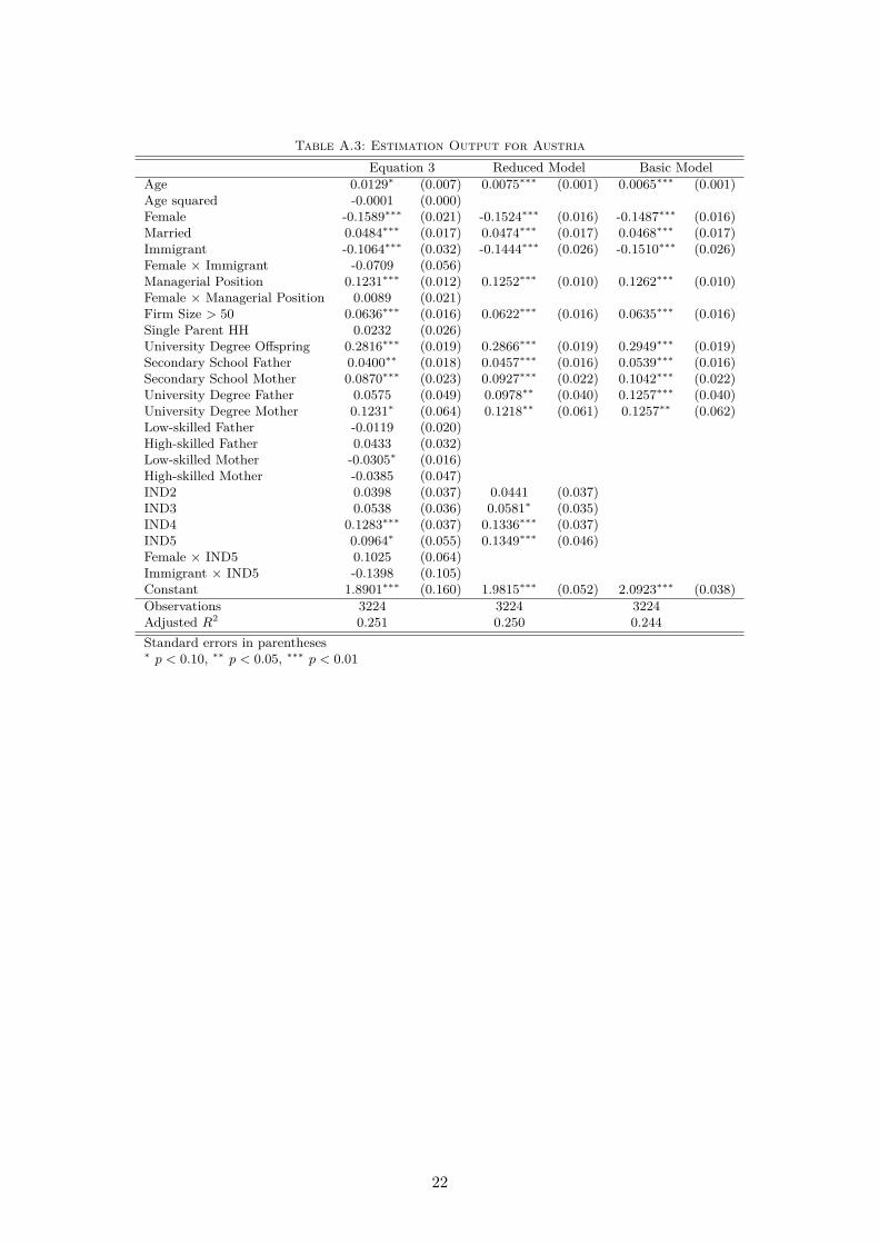
Table A.3: Estimation Output for AustriaEquation 3 Reduced Model Basic Model
Age 0.0129∗ (0.007) 0.0075∗∗∗ (0.001) 0.0065∗∗∗ (0.001)Age squared -0.0001 (0.000)Female -0.1589∗∗∗ (0.021) -0.1524∗∗∗ (0.016) -0.1487∗∗∗ (0.016)Married 0.0484∗∗∗ (0.017) 0.0474∗∗∗ (0.017) 0.0468∗∗∗ (0.017)Immigrant -0.1064∗∗∗ (0.032) -0.1444∗∗∗ (0.026) -0.1510∗∗∗ (0.026)Female × Immigrant -0.0709 (0.056)Managerial Position 0.1231∗∗∗ (0.012) 0.1252∗∗∗ (0.010) 0.1262∗∗∗ (0.010)Female × Managerial Position 0.0089 (0.021)Firm Size > 50 0.0636∗∗∗ (0.016) 0.0622∗∗∗ (0.016) 0.0635∗∗∗ (0.016)Single Parent HH 0.0232 (0.026)University Degree Offspring 0.2816∗∗∗ (0.019) 0.2866∗∗∗ (0.019) 0.2949∗∗∗ (0.019)Secondary School Father 0.0400∗∗ (0.018) 0.0457∗∗∗ (0.016) 0.0539∗∗∗ (0.016)Secondary School Mother 0.0870∗∗∗ (0.023) 0.0927∗∗∗ (0.022) 0.1042∗∗∗ (0.022)University Degree Father 0.0575 (0.049) 0.0978∗∗ (0.040) 0.1257∗∗∗ (0.040)University Degree Mother 0.1231∗ (0.064) 0.1218∗∗ (0.061) 0.1257∗∗ (0.062)Low-skilled Father -0.0119 (0.020)High-skilled Father 0.0433 (0.032)Low-skilled Mother -0.0305∗ (0.016)High-skilled Mother -0.0385 (0.047)IND2 0.0398 (0.037) 0.0441 (0.037)IND3 0.0538 (0.036) 0.0581∗ (0.035)IND4 0.1283∗∗∗ (0.037) 0.1336∗∗∗ (0.037)IND5 0.0964∗ (0.055) 0.1349∗∗∗ (0.046)Female × IND5 0.1025 (0.064)Immigrant × IND5 -0.1398 (0.105)Constant 1.8901∗∗∗ (0.160) 1.9815∗∗∗ (0.052) 2.0923∗∗∗ (0.038)Observations 3224 3224 3224Adjusted R2 0.251 0.250 0.244Standard errors in parentheses∗ p < 0.10, ∗∗ p < 0.05, ∗∗∗ p < 0.01
22
0
0
0.2
.2
.2.4
.4
.4.6
.6
.6.8
.8
.811
1Full-Time Employment in %
Full-
Tim
e Em
ploy
men
t in
%
Full-Time Employment in %AT
AT
ATBE
BE
BECY
CY
CYCZ
CZ
CZDK
DK
DKEE
EE
EEFI
FI
FIFR
FR
FRHU
HU
HUIE
IE
IEIS
IS
ISLT
LT
LTLU
LU
LUNL
NL
NLNO
NO
NOPL
PL
PLSE
SE
SESI
SI
SISK
SK
SKUK
UK
UKEU-SILC
EU-SILC
EU-SILCEurostat
Eurostat
Eurostat
Figure A.1: EU-SILC and Official Data on Full-Time Employment
Figure A.2: Annual Gross Wages in EU-SILC 2005 and Wage Tax Statistics 2004
-.1
-.1
-.10
0
0.1
.1
.1.2
.2
.2.3
.3
.3.4.4
.4Income Effect
Inco
me
Effe
ct
Income EffectLU***
LU***
LU***CY***
CY***
CY***CZ***
CZ***
CZ***AT***
AT***
AT***IT***
IT***
IT***ES***
ES***
ES***IS
IS
ISPL***
PL***
PL***BE***
BE***
BE***UK**
UK**
UK**SK**
SK**
SK**NO
NO
NONL*
NL*
NL*SI
SI
SILT**
LT**
LT**SE
SE
SEFR**
FR**
FR**IE
IE
IEEE
EE
EEHU
HU
HUDK
DK
DKFI
FI
FI
(Significance levels: ∗∗∗ 1%, ∗∗ 5%, ∗ 10%)
Figure A.3: Income Effects of Parental Income Status Movement from 1 to 5
23
0.2 0.4 0.6 0.8
−0.
20.
00.
20.
4
●
●
●
●
●
●
●
●
●
Plot for LU
0.2 0.4 0.6 0.8
−0.
20.
00.
20.
4
●
●
●
●
●
●
●
●
●
Plot for CY
0.2 0.4 0.6 0.8
−0.
20.
00.
20.
4
●●
●
●
●
●
●
●
●
Plot for CZ
0.2 0.4 0.6 0.8
−0.
20.
00.
20.
4
●●
●
●
●●
●
●
●
Plot for AT
0.2 0.4 0.6 0.8
−0.
20.
00.
20.
4
●
●
●●
●
● ●
●
●
Plot for IT
0.2 0.4 0.6 0.8
−0.
20.
00.
20.
4
●
●
● ●
●
●
●
●
●
Plot for PL
0.2 0.4 0.6 0.8
−0.
20.
00.
20.
4
●
●●
●●
●
●
●
●
Plot for ES
0.2 0.4 0.6 0.8
−0.
20.
00.
20.
4
●
●
●
●
●
●
●
●
●
Plot for IS
0.2 0.4 0.6 0.8
−0.
20.
00.
20.
4
●
●
●
●●
●●
●
●
Plot for SK
0.2 0.4 0.6 0.8
−0.
20.
00.
20.
4
●
●
●
●
●
●
●
●
●
Plot for BE
0.2 0.4 0.6 0.8
−0.
20.
00.
20.
4
●
●
●
●
●
●
●
●
●
Plot for NO
0.2 0.4 0.6 0.8
−0.
20.
00.
20.
4
●
●
●
●
●
●
●
●
●
Plot for SI
0.2 0.4 0.6 0.8
−0.
20.
00.
20.
4
●●
●
●
●●
●
●
●
Plot for NL
0.2 0.4 0.6 0.8
−0.
20.
00.
20.
4
●
●
●
●
●
●
●
● ●
Plot for HU
0.2 0.4 0.6 0.8
−0.
20.
00.
20.
4
●●
●
●●
●●
●
●
Plot for LT
24
0.2 0.4 0.6 0.8
−0.
20.
00.
20.
4
●
●
●
●
●
●
●
●●
Plot for IE
0.2 0.4 0.6 0.8
−0.
20.
00.
20.
4
●
●
●
●
●
●
●
●
●
Plot for SE
0.2 0.4 0.6 0.8
−0.
20.
00.
20.
4
●
●
●
●
●
●
●
●
●
Plot for FR
0.2 0.4 0.6 0.8
−0.
20.
00.
20.
4
●
●
● ●
●
●
●
●
●
Plot for EE
0.2 0.4 0.6 0.8
−0.
20.
00.
20.
4
●
●
●
●
● ●
●
●
●
Plot for DK
0.2 0.4 0.6 0.8
−0.
20.
00.
20.
4
●
●
●●
●●
●
●
●
Plot for FI
Figure A.4: Quantile Regression Results for Deciles
25