Interference Management for Stabilizationof Dynamical Systems over Wireless

Channels

IBRAHIM BILAL

Supervisor: Ali Abbas Zaidi

Examiner: Dr. Tobias Oechtering

Masters’ Degree ProjectStockholm, Sweden Aug 2012

XR-EE-KT 2012:002

To my parents

i

Table of Contents

Table of Contents ii

Abstract iv

1 Introduction 1

1.1 Motivation . . . . . . . . . . . . . . . . . . . . . . . . . . . . . . . . . . . . . . . . . 11.2 Background . . . . . . . . . . . . . . . . . . . . . . . . . . . . . . . . . . . . . . . . . 2

1.2.1 State Space Description of Dynamical Systems . . . . . . . . . . . . . . . . . 21.2.2 Control Theory . . . . . . . . . . . . . . . . . . . . . . . . . . . . . . . . . . . 31.2.3 Networked Control Systems . . . . . . . . . . . . . . . . . . . . . . . . . . . . 4

1.3 Related Work . . . . . . . . . . . . . . . . . . . . . . . . . . . . . . . . . . . . . . . . 101.4 Outline . . . . . . . . . . . . . . . . . . . . . . . . . . . . . . . . . . . . . . . . . . . 11

1.4.1 Chapter 2 . . . . . . . . . . . . . . . . . . . . . . . . . . . . . . . . . . . . . . 111.4.2 Chapter 3 . . . . . . . . . . . . . . . . . . . . . . . . . . . . . . . . . . . . . . 111.4.3 Chapter 4 . . . . . . . . . . . . . . . . . . . . . . . . . . . . . . . . . . . . . . 12

2 Control over Single User Interference Channel 13

2.1 Introduction . . . . . . . . . . . . . . . . . . . . . . . . . . . . . . . . . . . . . . . . . 132.2 Problem Formulation . . . . . . . . . . . . . . . . . . . . . . . . . . . . . . . . . . . . 14

2.2.1 Linear Sensing and Control . . . . . . . . . . . . . . . . . . . . . . . . . . . . 152.3 Main Results . . . . . . . . . . . . . . . . . . . . . . . . . . . . . . . . . . . . . . . . 172.4 Proofs . . . . . . . . . . . . . . . . . . . . . . . . . . . . . . . . . . . . . . . . . . . . 18

2.4.1 Proof of Theorem 2.2 . . . . . . . . . . . . . . . . . . . . . . . . . . . . . . . 182.4.2 Using delayed values of interference . . . . . . . . . . . . . . . . . . . . . . . 202.4.3 Proof of Theorem 2.3 . . . . . . . . . . . . . . . . . . . . . . . . . . . . . . . 21

2.5 Numerical Results and Discussion . . . . . . . . . . . . . . . . . . . . . . . . . . . . . 24

3 Control Over Two User Interference Channel 29

3.1 Introduction . . . . . . . . . . . . . . . . . . . . . . . . . . . . . . . . . . . . . . . . . 293.2 Problem Formulation . . . . . . . . . . . . . . . . . . . . . . . . . . . . . . . . . . . . 303.3 Main Results . . . . . . . . . . . . . . . . . . . . . . . . . . . . . . . . . . . . . . . . 313.4 Sensing and Control Scheme . . . . . . . . . . . . . . . . . . . . . . . . . . . . . . . . 32

3.4.1 Stability Analysis . . . . . . . . . . . . . . . . . . . . . . . . . . . . . . . . . . 343.5 Numerical Results and Discussion . . . . . . . . . . . . . . . . . . . . . . . . . . . . . 39

4 Conclusion and Future Work 48

ii

A Appendices in Chapter 2 50

A.1 Concavity w.r.t c . . . . . . . . . . . . . . . . . . . . . . . . . . . . . . . . . . . . . . 50A.2 Optimal c in Interference Pre-Cancelation . . . . . . . . . . . . . . . . . . . . . . . . 52A.3 Optimality in Sum Power Constraint . . . . . . . . . . . . . . . . . . . . . . . . . . . 53

Bibliography 55

iii

Abstract

In networked control systems, dynamical systems are stabilized by actions of remotely placed con-

trollers. This involves communication between plants and controllers over wireless channel(s). The

communication channel(s) are subjected to interfering signals, caused by some external radio de-

vices in the neighborhood or by the other wireless components within the same networked control

system. Interference in the communication channel is a major problem which drastically affects

performance of the dynamical systems that are to be controlled over the wireless channels. This

thesis in particular focuses on such a problem; it aims to improve stabilizability of linear systems by

managing interference in the wireless channels. We propose an idea of using dedicated sensor nodes

in a networked control system whose sole purpose is to manage interferences. Such a dedicated

sensor node is termed as a relay node in this thesis, as it relays its received information to the other

components in networked control system.

We assume first order linear time invariant plants with arbitrary distributed initial state and

model all the communication links as white Gaussian channels. We study two related setups. In the

first setup, we study the remote stabilization of a first order linear plant over a wireless channel in

which the communication between the plant’s sensor (state encoder) and controller is disturbed by

an independent interference signal. The relay node observes this interference information and sends

it to the state encoder and the controller, which then utilize this information to mitigate interference.

In the second setup, we consider two separate plants that communicate with two separate controllers

using a shared spectrum. Due to the common communication medium, the signals transmitted by the

state encoders of the two plants interfere with each other. In this setup, the relay node observes the

signals transmitted by the encoders of both plants. It then assists by communicating its observations

to the two controllers. The fundamental difference between the two setups is that in the former,

the interference is independent of the signal transmitted by the encoder, whereas in the later, the

interference becomes correlated with the signals transmitted by the encoders of the two plants. In

both setups, we use delay-free linear sensing and control schemes. By employing these schemes, we

derive sufficient conditions for mean square stability. We show that the achievable stability region

significantly enlarges with the relay assisted interference cancelation schemes.

iv

Chapter 1

Introduction

1.1 Motivation

Nearly every industrial plant requires some kind of regulation and control. Numerous applications

and services around the globe such as factory automation, space exploration, robots and automo-

biles incorporate control systems. These applications consist of dynamical systems whose response

is varying with time. Control systems are designed to influence and control this response by ma-

nipulating the input to the system. In many control problems, we deal with a scenario in which we

want to remotely control a dynamical plant over a given communication channel. The communi-

cation channel between the plant and controller imposes communication constraints on the control

performance. The system response is affected by quantization loss, packet drops, fading, thermal

noise, external interferences etc. Interference management is a key challenge in control problems

and is the emphasis of this thesis.

In networked control systems, a network of sensors and controllers is employed that act in co-

ordination to control the system. The sensor nodes (termed as relay nodes in this thesis) can have

partial or complete information of the system response and the interfering source. Having this in-

formation, the relay nodes mutually assist each other and other nodes in the network to minimize

the disturbances and uncertainties in the communication. In modern control applications such as

sensor networks, there are multiple plants that we desire to control simultaneously. This problem

is characterized as designing an optimal relaying scheme that decides on what information signal to

send and optimal controller scheme that decides on what control action to take in order to control

the remote plants.

1

2

This thesis in particular aims to solve such problems. We study the control problem of a single

as well as multiple plants. We design different relaying schemes in order to minimize the effect of

interferences and improve the control performance. The main goal of the thesis is to derive sufficient

conditions for remote control of the dynamical plants over a given channel.

1.2 Background

In this section, we explain the key concepts necessary to grasp the contents of this thesis. We begin

by defining dynamical systems, relate it to a basic control system and elucidate with a standard

example. Later on, we introduce networked control system and explain its constituents in detail.

We end the section by studying a classical problem of networked control systems.

1.2.1 State Space Description of Dynamical Systems

Dynamical systems are systems that evolve in time according to a fixed rule. At any point in time,

a dynamical system has a state vector which is referred to as a set of variables, also known as

the state variables that completely define the behavior of the system and its response to a given

input. A swinging pendulum is a typical example of a dynamical system. The state of the system

is the angular velocity and the angle where as the fixed rule or the evolution rule of this system is

Newton’s second law of motion. The state-space model of a discrete time closed loop linear time

variant system is of the form:

Xt+1 = f(x, u, t) = AtXt +BtUt, (1.1a)

Yt = CtXt +DtUt, (1.1b)

where Xt, Ut and Yt are the state, input and output vectors simultaneously. The matrices At and Bt

are system matrices defined by the system structure and elements. The matrix Ct is output matrix

which expresses the relation between state and output. The matrix Dt is feed forward matrix which

allows the control system to influence the output directly. In this state space model, (1.1a) is termed

as state equation in which the state vector Xt+1 is represented as a linear vector function f(x, u, t).

The output vector is a linear combination of Xt and Ut and is represented by the measurement

equation (1.1b). The measurement equation does not necessarily include all variables; in most of the

3

cases we choose Dt = 0. From the model in (1.1), we see that the state space equations completely

describe the system for all t if the initial conditions X0 and the inputs Ut for t ≥ 0 are known.

In this thesis we consider a time invariant system model, that is the matrices A, B and C

are constants. In this case, the mathematical manipulation of the state space equations yields the

transfer function between the output vector Y (z) and input vector U(z) as

H(z) =C adj(zI−A)B+ det(zI−A)D

det(zI−A).

It is seen that the eigenvalues of the matrix A are the poles of the system and determine system

stability. We will discuss system stability later in the section.

1.2.2 Control Theory

Control theory is branch of science that deals with the control and regulation of dynamical systems.

Control systems are employed in applications where we desire to influence the behavior of a dynamical

plant. In typical control problems, we are interested in adjusting the plant’s output according to

a given reference signal. In this problem, the controller aims to make sure that the state variable

does not exceed pre-specified thresholds. A standard example is that of a car cruise control. The

car encounters different terrains and elevations and one aims to design a system that keeps the

velocity at a desired level. A straight forward solution is to keep the throttle at a constant level.

However if the car is moving downhill or uphill, the velocity cannot be stabilized with this solution.

In this system, the measurement of the velocity (i.e. the state variable) is not used to control the

state variable. Such a system in which the controller is not fed with the output of the system it

is controlling, is termed as an open loop system. One can employ a feedback mechanism in which

the controller is fed with the state measurement. Based on the current measurement of the state

variable(s), the feedback controller can manipulate the dynamical plant in order to have a desired

effect on the output Xt of the system. Extending this to our example, the controller can increase or

decrease engine power in order to keep the velocity at the desired level. Such a system is termed as

a closed loop system.

We depict our example in Fig. 1.1 where the objective is to maintain the velocity of the car

to the reference variable r. The plant generates state Xt which is measured by a sensor (S). The

variable is then compared with the reference signal r. The difference between the reference and the

4

C

S

Xtr Utet+

− Plant

Figure 1.1: A simple closed loop cruise control system.

state variable is used by the controller C to take decision Ut in order to manipulate the state of the

dynamical plant at next time stamp.

1.2.3 Networked Control Systems

Networked Control Systems (NCS) are control systems in which a communication network is in-

volved. It consists of a set of sensors and controllers that have partial or complete access to the

state variable. The prominent examples of NCS are terrestrial exploration, aircrafts, manufactur-

ing plant monitoring, remote diagnostics and troubleshooting. In all of these examples, we aim to

control single or multiple plants through a remote feedback controller as shown in Fig. 1.2. In this

figure, the dynamical plants have an internal process noise W . Moreover, the communication link is

perturbed by external disturbance from a single or multiple interference sources. The set of sensors

are deployed in the network that help the communication between the plant and controller. In this

thesis the sensor nodes are termed as relay nodes R.

We are dealing with the field of stochastic control which means that the variables involved are

randomly distributed variables. The plant’s state as well as the interfering signals are all realizations

of stochastic variables. We now discuss the most fundamental control problem called the Linear

Quadratic Gaussian (LQG) Control.

Linear Quadratic Gaussian Control

The LQG control problem consists of a linear dynamical system that is to be controlled over an

additive white Gaussian noise (AWGN) channel. Moreover, the LQG control problem has a quadratic

5

R1 R1

Rk Rm

P1

P2

Pn

V1 V2 Vp

C1

C2

Cn

Wt

Controller NetworkPlant Network

Sensor Network Sensor Network

Interference Sources

......

......

. . .

Figure 1.2: A Networked control system closed over wireless channel.

criteria for design of optimal controller. In LQG problem we consider a linear system

Xt+1 = AXt +BUt +Wt, (1.2a)

Yt = CXt + Vt. (1.2b)

where Wt is the plants process and is Gaussian distributed variable with a given variance nw. The

controller receives the variable Yt after it is distorted by the i.i.d. channel noise Vt∼N (0, Nv). The

goal in stochastic control is to design an optimal control action Ut that minimizes the cost function

J = E

[N−1∑

t=0

l(Xt, Yt, Ut)

]= E

[XT (N)Q0X(N)

]+

N−1∑

t=0

E

[(XT

t UTt

)(Q1 Q12

Q21 Q2

)(Xt

Ut

)], (1.3)

where Q0 ≥ 0, Q2 > 0 and

(Q1 Q12

Q21 Q2

)≥ 0 are specified weighting matrices. We see that the

quadratic criterion l(·) not only aims to minimize the energy of the state and control variables but

also their cross relation defined by E[XTt Q12Ut] and E[UT

t Q21Xt]. The optimal controller action

Ut = f(Y t0 ) in LQG with Gaussian distributed variables that minimizes the cost function J is well

6

known [17] to be

Ut = −LtXt, with (1.4a)

Lt =[BTSt+1B +Q2

]−1 [BTSt+1A+Q21

], (1.4b)

St = ATSt+1A+Q1 −[ATSt+1B +Q12

]× Lt, (1.4c)

SN = Q0, (1.4d)

where St is a matrix computed by backward recursion and Xt = E [Xt|Y t0 ] is an estimate of the

state variable, computed from the available measurements Y0 . . . Yt at the controller. In most of the

cases, we are not interested in the cross relations i.e, we choose Q12=Q21=0.

Stability

Stability is an important concept in the field of control systems. The control action of any dynamical

system translates to stability of the system. A dynamical system is considered unstable if the system

response in unbounded in the interval t ∈ [0,∞]. The system is asymptotically stable if the response

is bounded at t = ∞. In the state space model (1.1a) and (1.1b), the system is asymptotically stable

when the eigenvalues of matrix A are within the unit disc i.e, |λi| < 1 and is marginally stable when

|λi| = 1.

In the LQG control problem, we cannot measure the state Xt directly from the observation. Our

goal is then to estimate its value from the measurement signal Yt. To model a good estimate of Xt,

we replicate the equations in (1.2) to form a state space model

Xt+1 = AXt +BUt +Wt, (1.5)

and et+1 = AXt −AXt = Aet,

where et is the estimation error. We see that the plant will be unstable when the uncertainty et

increases with time. If the matrix A is stable then the error will converge to zero. On the other

hand, if A is unstable then the estimation error will grow with time leading to an unstable system.

To counter this problem, we introduce a correction term in (1.5)

Xt+1 = AXt +BUt +Wt +K(Yt − Yt),

7

where Yt = CXt and K is a given matrix. Notice that, when we have a good estimate of Xt then

Yt approaches Yt. However as the uncertainty et = Xt − Xt increases, the term K(Yt − Yt) helps

correct the error. The estimation error in this scenario is given by

et+1 = AXt −AXt +Wt −K(CXt + Vt −CXt) = (A−KC)et +Wt −KVt (1.6)

This leads to the Linear Quadratic Gaussian estimation problem i.e, the optimal control action in

LQG is the one that minimizes the estimation error,

JLQG = limT→∞

E[‖ et ‖2].

For a noise free system that is when Vt = Wt = 0, the estimation error in (1.6) indicates that

system stability depends on eigenvalues of A−KC. Note that the system is stabilizable even if A

is unstable.

We introduce the concept of mean square stability [21].

Definition 1.1. A system is said to be mean square stable if there exists a constant M<∞ so thatE[XT

t Xt] < M for all t.

In this thesis, we desire to bound the state variable in mean square sense. It translates to

choosing Q2 = 0 in the quadratic criterion given in (1.3). This leads to the optimal controller action

Ut = AXt from (1.4). Since we study scalar closed loop LTI systems in this thesis, the state equation

is given by

Xt+1 = λXt + Ut +Wt = λ(Xt − Xt) +Wt (1.7)

Point to Point LQG

We now study a simple point to point LQG control problem. Consider a scalar discrete time LTI

plant in Fig. 1.3 that is remotely controlled over a memoryless feedback Gaussian channel. The

system model is give in (1.7).

This kind of scenario is designed in two blocks. First block consists of an observer O and an

encoder E lumped together. The observer/encoder block receives the state variableXt from the plant

and sends it over the channel after encoding. The second block consists of a decoder D and controller

C lumped together which receives the encoded state variable corrupted by interference(s). The linear

plant has an initial state X0 which is a random variable with an arbitrary distribution. The plant

8

O EXt St D CRt

Ut

ZtWt

Plant

Figure 1.3: A linear plant is controlled over an AWGN channel.

under consideration often has an internal noise processW ∈ R. This is applicable to scenarios where

we have to consider noise from imprecise measurements and interaction between different components

of the plant. The noise processWt is modeled as a zero mean white Gaussian noise with variance nw.

In the presence of the noise process, the state variable is partially observed by the encoder. In the

figure, the encoder E receives the state variable Xt from the plant and transmits St = ft(Xt) where

ft is the encoder policy which satisfies the average power constraint limT→∞1T

∑T−1t=0 E[S2

t ] ≤ Ps.

The controller/decoder block receives a measurement vector Rt = St + Zt distorted by the channel

noise Zt ∼ N (0, N). The control action is defined by Ut = −λXt, where Xt = E[Xt|{Rt}t0] is the

estimate of the state variable.

This is a classical control problem of stabilizing a single plant over a memoryless additive white

Gaussian channel (AWGN). The sufficient and necessary conditions for stability of such a system is

computed in [3] as

log(λ) <1

2log

(1 +

Ps

N

), (1.8)

Relay Assisted Control:

Since we estimate the state variable at the controller, the interference noise power in the channel

is a major concern. One way to tackle this problem is to place multiple sensors in the network

that are dedicated to sense the interference and convey it to the controller and encoder. This type

of dedicated sensors will be referred as relays (R) throughout this thesis. There are number of

strategies on how to efficiently utilize the relays. A convenient approach is to place the relay node

close to the interferer. In this way, the relay node gains near perfect knowledge of the interference

which can be relayed to the encoder and controller nodes.

In most part of the thesis, we consider that the relay transmission is delay free. In a commu-

nication network, the authors of [5] study the relay without delay and derive an upper bound on

9

channel capacity. However in some practical systems, relay communication suffer from a delay which

imposes constraints on the transmission rates. The capacity bounds of such systems is derived in [6].

Potential gains in stability of a plant by employing dedicated sensors (relays) has attracted much

attention in modern control applications. In de-centralized control systems, there are multiple relay

nodes deployed which act in coordination to stabilize the plant. We have already shown a general

relay assisted scenario in Fig. 1.2. The communication between plant and controller network is

perturbed by an interfering signal Vt. To help the control problem, a network of relays is introduced

that exchange interference information between each other and other components of the network

through a separate link under an average power constraint. Using this information, the nodes in the

networked control system can reduce the uncertainties caused by the interferer.

Gaussian Interference Channels

Channel is defined as the transmission medium or connection between a sender and receiver over

which some information message is conveyed. If there is an additive white Gaussian noise (AWGN)

component present in the transmission medium, then such a channel is termed is a Gaussian inter-

ference channel.

RX1

RX2

T1

T2

h

h

Z2,t

Z1,t

X2,t

X1,t

Y2,t

Y1,t

Figure 1.4: A two user Gaussian interference channel with channel gain h and independent noiseterms Z1, Z2 ∼ N (0, N).

In Gaussian interference channels we have strict one to one correspondence between the sender

and receiver. In the case when two independent transmitter nodes send separate messages to separate

receivers over the same transmission medium, the channel is called a two user Gaussian interference

10

channel. In such a channel, the message from one transmitter to its corresponding receiver is

perturbed by the message from the other transmitter as shown in Fig. 1.4. The received messages

are

Y1,t = X1,t + hX2,t + Z1,t

Y2,t = X2,t + hX1,t + Z2,t

In this thesis we consider discrete time memoryless Gaussian channel. The channel in Fig. 1.4 is

said to be memoryless if the output at a particular instant is dependent on the input only at that

time, i.e,

p(Y1,0...tY2,0...t|X1,0...tX2,0...t) =t∏

i=0

p(Y1,iY2,i|X1,iX2,i).

1.3 Related Work

Recently, the field of control and communication has gained much attention. The communication

channel involved in the networked control system imposes communication constraints on the control

performance. The authors of [1, 16] have studied this relation between communication and control.

In [3], it is shown that the remote stabilization of a feedback control system is closely related to a

communication problem over the given channel. The stability of a system under data rate constraints

is studied in [15,20], where the authors have added a lower bound that characterizes the degradation

in performance resulting in reducing data rate. In [19], the necessary rate conditions for stability

of a control over noisy channel have been derived. The LQG control problem with communication

capacity constraints is studied in [10].

There has been significant research in control problems under signal-to-noise ratio constraint such

as the studies in [4, 12, 13, 23]. The authors of [18] study the stabilization over power-constrained

parallel Gaussian channels where they have derived the bounds on channel capacity for feedback

stabilization. In [22], the necessary and sufficient conditions for stability of control over memory

channels are derived. The stability conditions for control of LTI systems over varying feedback

channels are obtained in [14].

Some research studies consider the problem of control over fading channels. In [9], the authors

study Optimal LQG control over Gaussian fading channels. The research in [2] goes one step further

11

which derive the necessary and sufficient conditions for stability of continuous time linear Gaussian

systems over additive white noise wireless channels subject to capacity constraints.

Gaussian channel with multiple relay nodes is studied in [7] where they find the upper bound on

the capacity of such communication networks. In [24] the authors find memoryless relaying schemes

for maximizing transmission rates. Moreover, some non-linear relaying scheme have been shown

in [8] to achieve better data rates. This is a remarkable result since one can expect potential gain

in the stability by using such non-linear relaying schemes in networked control systems.

1.4 Outline

In this section we will give an outline of the report. We consider two different networked control

systems that are studied in separate chapters.

1.4.1 Chapter 2

In this chapter, we formally study the closed loop remote stabilization of a plant in the presence

of a single interferer that is modeled as a random variable with Gaussian distribution. We begin

with a linear relay assisted scheme in which the relay has perfect instantaneous knowledge of the

interference. The relay broadcasts interference information to the controller as well as the state

encoder. The encoder uses this information to pre-cancel the interference where as the controller

uses this information to post-cancel the interference. We investigate the gains in stability achieved

by using the relay assisted scheme and compare it with a system without relay. In the next step,

we will consider an ideal situation in which the encoder has complete future information of the

interference. Finally, we consider a realistic case in which the interference pre-cancelation is affected

by a delay. We derive the stability conditions for the mentioned schemes, analyze the results and

end the chapter with a discussion.

Related Publication : Ibrahim Bilal, A. A. Zaidi, T. Oechtering and M. Skoglund, “Interference

management for stabilization over wireless channels” in Proc. IEEE MSC 2012

1.4.2 Chapter 3

This chapter studies the problem of remote stabilization of two dynamical plants in a symmetric two

user Gaussian interference channel. This case is applicable to the scenarios where the interfering

12

source is output of another dynamical control system or a wireless device in the close vicinity. We

introduce a relay node that partially observes the state variables from the two plants. The relay

node helps the communication by forwarding a linear combination of the partially observed output

from the two plants. The controller nodes use the information from the relay and their respective

encoders to estimate the desired state variable. The objective of this chapter to derive sufficient

conditions for the mean square stability of the linear plants over the given channel.

1.4.3 Chapter 4

The final chapter gives a conclusion to the thesis work and discusses some research areas for future

work.

Chapter 2

Control over Single User

Interference Channel

2.1 Introduction

In this chapter we consider remote stabilization of a linear plant over a Gaussian channel subject

to an external interference signal. We introduce the idea of managing the external interference

by informing the plant’s sensor and the remote controller about the interference signal with the

help of a relay node. The relay node in the given setup is a communication device which relays the

interference information to the sensor and the controller under an average transmit power constraint.

Based on the interference information received via the relay, the plant’s sensor tries to pre-cancel

the interference under an average transmit power constraint and the remote controller tries to post-

cancel the interference. For understanding fundamental principles we have neglected the effect of

communication delays and assumed that the relay node fully observes the interference. In a practical

sensor networking scenario, the relay node can for example be an idle sensor node observing any

radio interference present in the environment.

In an industrial scenario, with challenging and time-varying interference patterns, such relay

nodes can also be deployed as dedicated to this purpose. In the coming sections, we will derive

necessary and sufficient conditions for mean square stability of the linear plant over the given com-

munication channel using some relay-assisted interference cancelation schemes. Moreover, we will

study the potential gains one can obtain by deploying a dedicated inexpensive sensor (relay) node

to manage interference in a network of control systems closed over wireless channels.

13

14

2.2 Problem Formulation

Consider a discrete-time LTI system in Fig. 2.1 with state equation

Xt+1 = λXt + Ut +Wt, (2.1)

where Xt ∈ R, Ut ∈ R, and Wt ∈ R are the state, control, and plant noise processes respectively.

The process noise {Wt} is a zero mean white Gaussian noise sequence with variance nw. The initial

state X0 is assumed to be a random variable having an arbitrary probability distribution with a

given variance α0. The open loop system is assumed to be unstable i.e, λ > 1. We consider a

remote control setup where a sensor node observes the state process and transmits it over a wireless

link to a remotely situated controller. In order to communicate the observed state value Xt, an

encoder E is integrated with the observer O and a decoder D is integrated with the controller

C as depicted in Fig. 2.1. The communication link from the state encoder to the controller is

assumed to be an additive white Gaussian noise channel, which is the simplest model for the wireless

channel. Generally the communication over wireless channels is subject to interference from other

users (sources) sharing the same radio spectrum. In this problem we consider a single interfering

source whose signal Vt interferes in an additive manner with the signal transmitted by the state

encoder as shown in Fig. 2.1. The interfering signal Vt is modeled as a white Gaussian sequence

having zero mean and variance Nv. In order to combat the interference, a sensor node is placed

adjacent to the interferer which is assumed to have a perfect observation of the interference. This

can be either seen as an idealistic assumption or the sensor node is part of the interferer. This

sensor then relays its observations to both the state encoder and the remote controller, therefore

we call it a relay node R. This relay node can also play a dual role by also assisting information

transmission in a secondary system which is causing interference to the primary system. However

the sole purpose of the relay node in this problem is to assist the state encoder and the controller

to combat the interference.

The communication and control protocol works as follows. At any time instant t, the relay node

R broadcasts the information of Vt to both state encoder E and the controller C by transmitting

Sr,t = γt(Vt), where γt : R× N 7→ R is the relay policy which satisfies an average power constraint

E[S2r,t] ≤ Pr. Accordingly the state encoder E receives Yt = Sr,t + Zr,t, where Zr,t ∼ N (0, Nr)

15

Plant O/E D/C

Yt

Se,t

Sr,t

R1,t

R2,t

Zr,t Zd,t

Zt

h

Xt

R

Ut

Vt

Vt

Figure 2.1: A linear plant has to be stabilized by the joint actions of observer/encoder (O/E) anddecoder/controller (D/C) over a Gaussian channel subject to an external interference signal. Arelay node R is deployed, whose purpose is to mitigate the effect of interference by informing E

and C about the interference.

is the noise component in R − E link. The state encoder then transmits Se,t = ft(Xt, Yt), where

ft : R2 × N 7→ R must satisfy an average transmit power constraint limT→∞

1T

∑T−1t=0 E[S2

e,t] ≤ Ps.

Accordingly the controller receives R1,t and R2,t from the state encoder and the relay respectively

R1,t = Se,t + Vt + Zt,

R2,t = hSr,t + Zd,t,

where Zt ∼ N (0, N) is the white noise component in E − C link, Zd,t ∼ N (0, Nd) is white the noise

component in R − D link, Vt ∼ N (0, Nv) is the interference variable, and h ∈ R is the gain of

R − D link. The interference variable Vt and the noise variables Zt, Zr,t and Zd,t are all mutually

independent for all time steps t. The controller takes an action based on the received signals,

Ut = πt({R1,i}ti=0, {R2,i}ti=0) where πt : R2(t+1) × N 7→ R is the decoder/controller policy. The

controller aims at stabilizing the system in mean square sense (see Def. 1.1).

The main objective we will attempt to achieve is to derive necessary and sufficient conditions for

mean square stability of the system in (2.1) over the given communication channel.

2.2.1 Linear Sensing and Control

In this section we introduce a delay-free linear and memoryless scheme for mean square stabilizing

the LTI system in (2.1). The sensing and control scheme works as follows. At any time t the

16

relay transmits Sr,t =√

Pr

NvVt. The sensor E observes the state Xt of the plant and it also receives

Yt = Sr,t + Zr,t from the relay. The encoder then transmits a linear combination of Xt and Yt

according to

Se,t =

√Ps

D

(Xt√αt

+ cYt√

Pr +Nr

), (2.2)

where c ∈ R is the interference combining coefficient and we choose D = 1 + c2 in order to ensure

the average transmit power constraint E[S2e,t

]= Ps. Accordingly the signals received by the remote

controller are given by

R2,t = hSr,t + Zd,t = h

√Pr

NvVt + Zd,t, (2.3)

R1,t = Se,t + Vt + Zt

(a)=

√Ps

DαtXt +

(1 + c

√k1Ps

DNv

)Vt + c

√Ps

D(Pr +Nr)Zr,t + Zt, (2.4)

where (a) follows from (2.2) and k1 := Pr

Pr+Nr. The decoder computes the minimum mean square

error (MMSE) estimate of the state as Xt = E [Xt|{R1,i}ti=0, {R2,i}ti=0] and applies the following

action on the plant; Ut = −λXt.

By choosing different values of the system and the communication channel parameters, we can

get some special cases. In the following we highlight two scenarios.

A. Relay-assisted Interference Pre-cancelation

This refers to the scenario where there is no direct communication link from the relay to the con-

troller, that is h = 0. In this case the relay is only assisting the state encoder to pre-cancel the

interference. The encoder has limited transmit power, which has to be used for transmission of the

state process and for the interference pre-cancelation.

B. Relay-assisted Interference Post-cancelation

This refers to the scenario where there is no direct communication link from the relay to the encoder

or the encoder does not utilize the information from the relay, that is we choose c = 0 in (2.2). In

this case the relay is only assisting the controller to post-cancel the interference.

17

2.3 Main Results

In this section we present some necessary and sufficient conditions for mean square stability of system

in (2.1).

Theorem 2.1. The scalar LTI system can be mean square stabilized over the given channel in theabsence of relay node if and only if

log(λ) <1

2log

(1 +

Ps

N +Nv

). (2.5)

Proof. In the absence of relay node, E − C link is a point-to-point channel with zero mean whiteGaussian noise having variance N + Nv. The necessary and sufficient condition for mean squarestabilization over this channel is given by (2.5), see for example [23].

Theorem 2.2. The scalar LTI system in (2.1) can be mean square stabilized in the presence of relaynode if

log(λ) <1

2log

(1 +

Ps

c⋆2Ps +D⋆ (N +Nv(2M − 1− k2M2))

), (2.6)

where M = 1 + c⋆√

k1Ps

D⋆Nv, D⋆ = 1 + c⋆2, k1 = Pr

Pr+Nr , k2 = h2Pr

h2Pr+Nd, and c⋆ is the unique real

solution of the following equation

2c(Ps +N +Nv(2M − 1− k2M

2))+ 2Nv

(√k1Ps

DNv(1 − k2M)

)= 0.

Proof. The proof is given in Section 2.4.

By choosing c = 0 and h = 0 in Theorem 2.2, we get stability results for the two special cases

given in Section 2.2.1.A and 2.2.1.B.

Corollary 2.1. The scalar LTI system in (2.1) can be mean square stabilized using the relay assistedinterference pre-cancelation scheme if

log(λ) <1

2log

(1 +

Ps

c⋆2Ps +D⋆(N +Nv) + 2c⋆√k1PsNvD⋆

), (2.7)

where c⋆ is given by

c⋆ = − 1√2

(−1 +

√(Ps +N +Nv)2

(Ps +N +Nv)2 − 4k1PsNv

) 1

2

.

Proof. The expression (2.7) follows from (2.6) by choosing h= 0. The optimal c⋆ is computed inA.2.

Corollary 2.2. The scalar LTI system in (2.1) can be mean square stabilized using the relay assistedinterference post-cancelation scheme if

log(λ) <1

2log

1 +Ps

N +Nv(

Nd

h2Pr+Nd

)

. (2.8)

18

Proof. The proof directly follows from (2.6) by choosing c = 0.

Remark 2.1. If we consider a special case of interference pre-cancelation (h=0) scheme, in which thestate encoder receives a delayed version of the interference information i.e, the relay node transmitsVt−1 instead of Vt, then such a scheme does not improve achievable stability region of the givensystem. A delay in interference information is not useful in improving control performance. Weshow in Section 2.4.2

Remark 2.2. If we impose a sum power constraint P = Ps+Pr on the interference post-cancelation(c=0) scheme, then the scheme has to optimally distribute power between the state encoder andrelay. In the sum power constraint, the relay assisted scheme performs at least as good as the relayless scheme. The optimal allocation {P ⋆

s , P⋆r } has been computed in A.3.

Remark 2.3. Note that one can completely eliminate the effect of interference using the post-cancelation scheme if R − D link is noiseless (Nd = 0). But we cannot eliminate the effect ofinterference by using the pre-cancelation scheme for noiseless R− E link (Nr = 0). However in thefollowing we present an ideal scenario where an interference pre-cancelation scheme can completelyeliminate the effect of interference.

Consider a scenario where the state-encoder E has a complete future information of the interfer-

ence. That is at time t = 0 the encoder has prior knowledge of Vi for all i ≥ t. For this case we have

the following necessary and sufficient condition.

Theorem 2.3. The scalar LTI system in (2.1) with Wt = 0 can be mean square stabilized overAWGN channel using non-causal information of the interference at the state encoder if

log(λ) <1

2log

(1 +

Ps

N

). (2.9)

Proof. The proof is given in Section 2.4.

2.4 Proofs

In this section we give proofs of Theorem 2.2 and Theorem 2.3.

2.4.1 Proof of Theorem 2.2

We use linear sensing and control scheme presented in Section 2.2.1 to derive sufficient condition for

stability.

Initial time step, t = 0: The encoder E observes X0 and transmits Se,0 =√

Ps

α0

X0. The decoder

D receives R1,0 = Se,0 + V0 + Z0 and estimates X0 =√

α0

PsR1,0. The controller takes controller

action U0 = −λX0. The next state in accordance with (2.1) is given by

X1 = λX0 + U0 +W0 = λ(X0 − X0) +W0

= −λ√α0

Ps(V0 + Z0) +W0.

19

Since X1 is a linear combination of zero mean mutually independent Gaussian variables (V0, Z0,W0),

therefore it is a Gaussian distributed random variable with variance

α1 = E[X21 ] = λ2

α0

Ps(Nv +N) + nw.

For time steps, t ≥ 1: The relay node R observes Yt and broadcasts Sr,t =√

Pr

NvVt which is

received by the state encoder as Yt = Sr,t + Zr,t. The encoder transmits Se,t according to (2.2).

The decoder observes R1,t and R2,t in accordance with (2.4) and (2.3) respectively. The decoder

computes an estimate of the state Xt as

Xt = E[Xt|{R1,i}ti=0, {R2,i}ti=0]

(a)= E[Xt|R1,t, R2,t]

(b)= l1R1,t + l2R2,t,

where (a) follows from the orthogonality property of MMSE estimate that is E[XtR1,t−j ] = E[XtR2,t−j ] =

0 for j ≥ 1; (b) follows from the fact that the optimum MMSE estimate of a Gaussian variable is

linear. The computation of the estimator coefficients l1, l2 ∈ R gives

l1 =1

G

√αtPs

D, l2 = − hM

√αtPsPrNv

(h2Pr +Nd)G√D,

where we have defined G := Ps +N +Nv(2M − 1− k2M2). The second moment of state process is

then given by

αt+1 = E[X2t+1] = E

[(λ(Xt − Xt) +Wt

)2]

(a)= λ2

(E[X2

t ]+E[X2t ]−2E[XtXt]

)+E[W 2

t ]

(b)= λ2

(αt + αt

Ps

DG− 2αt

Ps

DG

)+ nw

= αt

[λ2(DG− Ps

DG

)]+ nw (2.10)

(c)= α0

[λ2(DG− Ps

DG

)]t+nw

t−1∑

i=0

(λ2DG− Ps

DG

)i

, (2.11)

where (a) follows from the fact that {Wt} is a sequence of i.i.d. random variables and is independent

of {Xt, Xt}; (b) follows from E[XtXt] = E[X2t ] = αt

Ps

DG by computation and (c) follows by recursively

applying (2.10). Now we wish to find a condition which guarantees boundedness of {αt} for all t ≥ 0.

We observe from (2.11) that αt converges to a constant real number as t→ ∞ if

λ2(DG− Ps

DG

)< 1 ⇒ log(λ) <

1

2log

(1 +

Ps

DG− Ps

).

20

By substituting G=Ps+N+Nv(2M−1−k2M2), we obtain the sufficient condition in (2.6)

log(λ) <1

2log

(1 +

Ps

c2Ps +D (N +Nv(2M − 1− k2M2))

). (2.12)

We now consider the right side of the inequality in (2.12) and show in A.1 that this is concave with

respect to c.

2.4.2 Using delayed values of interference

In practical systems, the interference information received at the encoder might suffer from a time

delay. In this section, we consider a subcase of interference pre-cancelation in which the relay

transmits one step delayed instantaneous interference information Vt−1 to the state encoder. We

aim to show that the using delayed version of interference variable does not help in improving system

stability. To keep things simple, we assume that the interference information received by the state

encoder is perfect i.e, Nr = 0.

Initial time step, t = 0: The state encoder transmits Se,0 =√

Ps

α0

X0. The decoder receives

R1,0 = S1,0 + V0 + Z0 and computes X0 =√

α0

PsR1,0. The controller takes the action U0 = −λX0.

The state variable at next time stamp is

X1 = λX0 + U0 +W0 = −λ√α0

Ps(V0 + Z0) +W0.

Time steps, t ≥ 1: The state encoder observes Xt and receives one step delayed perfect interference

information Vt−1 from the relay node. The state encoder transmits a linear combination of the state

and interference variables

Se,t =

√Ps

Dt

(Xt√αt

+ cVt−1√Nv

), (2.13)

where Dt = 1+ c2 +2cρt. Note that Xt in (2.13) is not independent of the interference information

Vt−1 sent by the encoder. We have therefore introduced the correlation coefficient ρt =E[XtVt−1]√

αtNvin

Dt to ensure the average power constraint E[S2e,t

]= Ps. The decoder receives R1,t = S1,t + Vt +Zt

and computes an estimate of the state as

Xt = E[Xt|R1,t](a)=

E[XtR1,t]

E[R21,t]

Rt, (2.14)

21

where (a) follows from the orthogonality principle of MMSE estimate. The second moment of the

state variable is given as

λ2t+1 =E[X2t+1] = E

[(λ(Xt − Xt) +Wt

)2],

(a)=λ2

[E[X2

t ]E[R21,t]− E[XtR1,t]

E[R21,t]

]+ nw,

(b)=αt

[λ2

(Ps +N +Nv)Dt − Ps(1 + cρt)2]

(Ps +N +Nv)Dt

]+ nw, (2.15)

where (a) follows from (2.14) and (b) follows from E[XtR1,t] =√

Psαt

Dt(1 + cρt) and E[R2

t ] = Ps +

N+Nv by computation. Comparing (2.15) with αt for the without relay scheme in (2.5), we observe

that using one step delayed interference information is useful if

(Ps +N +Nv)Dt − Ps(1 + cρt)2

(Ps +N +Nv)Dt<

N +Nv

Ps +N +Nv.

Simplifying the above inequality, we obtain

Ps

(Dt − (1 + cρt)

2)< 0

⇒ Psc2(1− ρt)

2 < 0,

which never holds since c ∈ R. This shows that using delayed version of interference information for

pre-cancelation is not useful in stabilizing the system.

2.4.3 Proof of Theorem 2.3

Consider that the plant in (2.1) is noiseless i.e Wt = 0, and further assume that the state encoder

at time t = 0 knows Vi for all i > 0. In this setup, we do not consider any assistance from the

relay node. We propose a linear sensing and control scheme based on the coding scheme in [11], and

derive sufficient condition in (2.9). We first define the following variables:

β : =√1 + Ps/N, g :=

√Ps/N , and

ψi+1 = ψi +

(1− 1

β2

)Viβig

, (2.16)

φi+1 =1

β2φi +

(1− 1

β2

)Zi

βig, (2.17)

22

with ψ1 := V0/β and φ1 := Z0/β. The channel noise {Zt} is a zero mean i.i.d. Gaussian sequence

therefore {φi} is also Gaussian. We compute the variance of φi by induction. For i = 0

E[φ21] = E[Z20 ]/β

2 = N/β2.

We claim that E[φ2t ] = N/β2t for all t ≥ 1. Assuming that our argument is correct then

E[φ2t+1] =1

β4E[φ2t ] +

(1− 1

β2

)2E[Z2

t ]

β2tg2

=1

β4

(N

β2t

)+

(g2

β2

)2N

β2tg2

=N

β2tβ4(1 + g2) =

N

β2(t+1), (2.18)

which validates our argument by induction.

The linear sensing and control scheme works as follows.

Initial transmission, t=0 : The encoder E observes X0 and transmits Se,0 = −β(X0 + ψn),

where ψn is computed by the encoder according to (2.16) from the non-causal information of Vt for

t = 0, 1, . . . , n. The decoder D observes

R1,0 = −β(X0 + ψn) + V0 + Z0,

and estimates the initial state as

X0|0 = −R1,0/β = X0 + ψn − 1

β(V0 + Z0)

= X0 + ψn − ψ1 − φ1,

where X0|0 is the estimate of the initial state X0 at time t = 0. The controller C takes an action

U0 = −λX0|0 on the plant which results in

X1 = λX0 + U0 = λ(X0 − X0|0) = λ(−ψn + ψ1 + φ1).

Further transmission t ≥ 1: The encoder E observes Xt and transmits Se,t = −βtgλt (Xt+λ

t(ψn−

ψt)). We observe that the encoder adds λt(ψn − ψt) to Xt before transmission in order to save

transmit power by canceling the contribution of {Vt} in the state process. Shortly, we will show that

Se,t satisfies the average power constraint E[S2e,t]=Ps. The controller receives R1,t = Se,t + Vt +Zt,

and computes the estimate X0|t as

X0|t = X0|t−1 −(1− 1

β2

)Rt

βtg.

23

The controller takes the following action

Ut = λt+1(X0|t−1 − X0|t). (2.19)

The plant’s next state Xt+1 is given by

Xt+1 =λXt + Ut

(a)=λ

(λt(X0 − X0|t−1)

)+ λt+1(X0|t−1 − X0|t)

=λt+1(X0 − X0|t), (2.20)

where (a) follows from (2.19).

We now show by induction that from the above scheme, X0|t = X0+ψn−ψt+1−φt+1. At t = 1,

we have

Se,1 =− βg

λ(X1 + λ(ψn − ψ1)) = −βgφ1.

X0|1 =X0|0 −(1− 1

β2

)R1

βg

(a)=(X0 + ψn − ψ1 − φ1

)+

(1− 1

β2

)φ1 −

1

βg

(1− 1

β2

)(V1 + Z1)

(b)=X0 + ψn − ψ2 − φ2,

where (a) follows from substituting R1,1 = Se,1 + V1 + Z1 and (b) follows from (2.16) and (2.17).

The next state then is computed as

X2 = λ2(X0 − X0|1) = λ2(−ψn + ψ2 + φ2).

Assuming that our argument X0|t−1 = X0 + ψn − ψt − φt is true for t ≥ 1 then for the next time

step

Se,t =− βtg

λt(Xt + λt(ψn − ψt)) = −βtgφt.

X0|t =X0|t−1 −(1− 1

β2

)Rt

βtg

=(X0 + ψn − ψt − φt

)+

(1− 1

β2

)φt −

1

βtg

(1− 1

β2

)(Vt + Zt)

=X0 + ψn − ψt+1 − φt+1, (2.21)

24

which validates our induction that X0|t =X0 + ψn−ψt+1−φt+1 at all times t ≥ 0. It can be seen

that Se,t=−βtgφt for t ≥ 1 which gives

E[S2e,t] = β2tg2E[φ2t ]

(a)= g2N = Ps,

where (a) follows from (2.18). This satisfies the average power constraint limT→∞1T

∑T−1t=0 E[S2

e,t] ≤

Ps. With the proposed scheme above, it follows from (2.20) and (2.21) that at all times

Xt+1 = λt+1(−ψn + ψt+1 + φt+1). (2.22)

If we let n = t+1, then the plant’s state according to (2.22) is Xt+1 = λt+1φt+1. The second moment

of the state process is then given by

E[X2t+1] = αt+1 = N

(λ2

β2

)t+1

,

from which we observe that αt → 0 as t→ ∞ if

λ2

β2< 1 ⇒ log(λ) <

1

2log

(1 +

Ps

N

).

This completes the proof of Theorem 2.3. �

Remark 2.4. The probability distribution of the interference Vt has no significance in derivingthe sufficient conditions. This implies that the theorem will hold true for any i.i.d. sequence ofinterference.

Remark 2.5. The non-causal information of interference is utilized only in computation of ψn. Ifthe number ψn is already computed and known, the encoder does not need to know future values ofinterference.

2.5 Numerical Results and Discussion

We know from Section 2.2.1 that the system stabilization is influenced by the following set of

communication variables: {N,Nv, Nd, Nr, Ps, Pr}. Therefore we study and discuss the effect of

these variables. We consider the following schemes: i) the generic relay scheme (i.e, when both

the state encoder and controller utilize interference information), ii) the interference pre-cancelation

(h=0) scheme, iii) the interference post-cancelation (c=0) scheme and iv) the relayless scheme. The

stability regions achieved using these schemes are given in (2.6), (2.7), (2.8) and (2.5) respectively.

For the sake of reference we will also consider v) without interference scheme according to (2.9).

25

0 2 4 6 8 100

0.02

0.04

0.06

0.08

0.1

0.12

0.14

0.16

Generic Relay Post−Cancelation (c=0) Pre−Cancelation (h=0) Without Relay Without Interference

log10(λ)

Interference Noise Power, Nv

Figure 2.2: Achievable stability regions for various cases plotted as functions of Interference noisepower Nv, with N=Nr=Nd=1 and Ps=Pr=5.

Note that this scheme serves as an upper bound on attainable stabilizability and can be achieved

according to Theorem 2.3 when the interference is non-causally known at the encoder. In Fig. 2.2

we fix Nd = 0.5, Nr = 0.25, h=N=Ps=Pr=1 and plot the boundary of the achievable stability

regions for the above mentioned schemes as functions of interference noise power Nv. We observe

that the use of relay can substantially improve the system stabilizability. The generic relay case is

as at least as good as the two sub-cases, namely interference pre-cancelation (h=0) and interference

post-cancelation (c=0) scheme. In high interference regime, the pre-cancelation (h=0) scheme

outperforms the post-cancelation (c=0) scheme. The gap between the achievable stability region for

the two schemes enlarges significantly as Nv increases. This is due to the reason that the transmit

power available at the state encoder is not enough to pre-cancel the high interference. In the high

interference scenario, the achievable stability region for the interference pre-cancelation (h=0) scheme

eventually approaches that of the relayless scheme. The pre-cancelation scheme in this situation no

longer remains useful and consequently, the stability region for the generic relay scheme approaches

the post-cancelation (c=0) scheme.

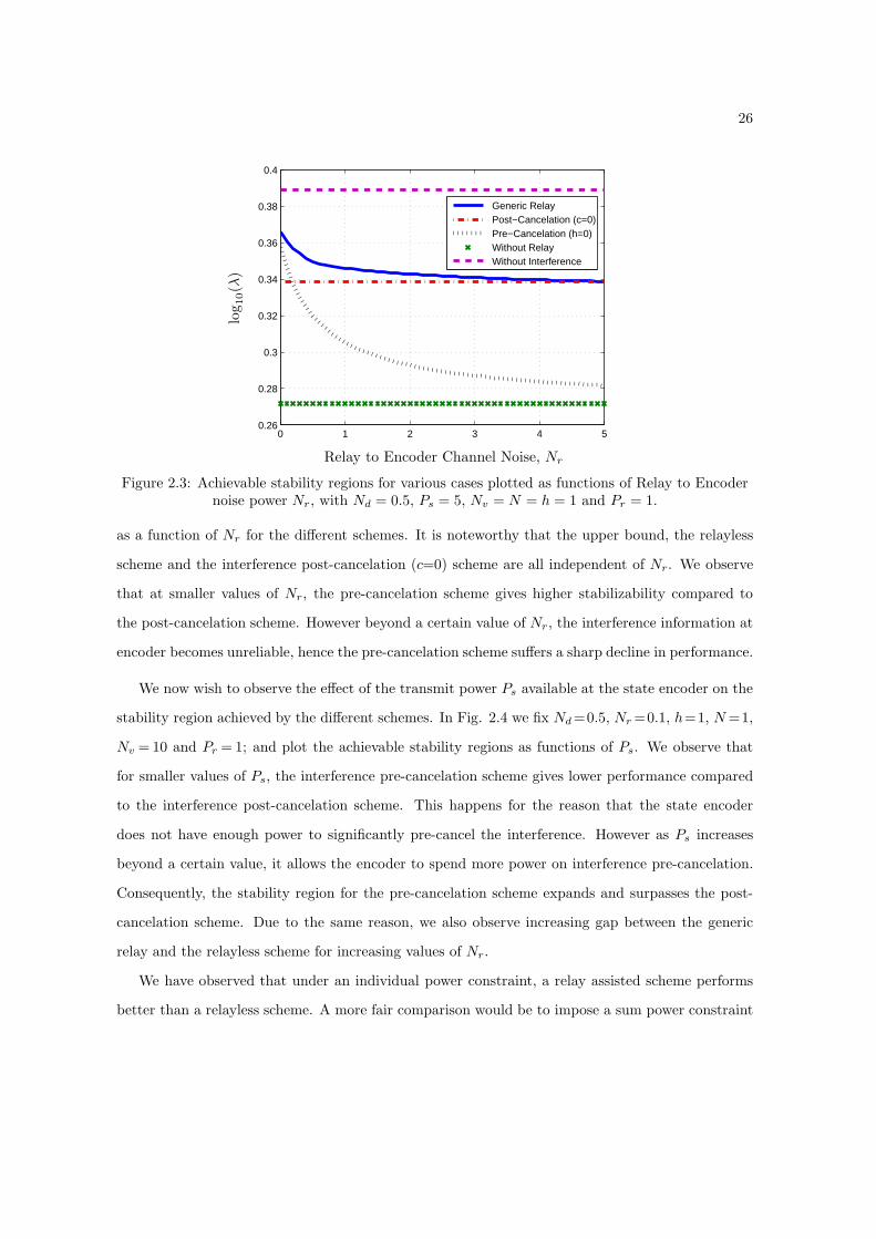
The reliability of the interference information at the state encoder depends on the quality of the

R− E link, therefore we study the effect of the channel noise power Nr on system stability. In Fig.

2.3 we fix Nd = 0.5, h= 1, N = 1, Nv = 1, Ps =5, Pr = 1, and plot the attainable stability regions

26

0 1 2 3 4 50.26

0.28

0.3

0.32

0.34

0.36

0.38

0.4

Generic Relay Post−Cancelation (c=0) Pre−Cancelation (h=0) Without Relay Without Interference

log10(λ)

Relay to Encoder Channel Noise, Nr

Figure 2.3: Achievable stability regions for various cases plotted as functions of Relay to Encodernoise power Nr, with Nd = 0.5, Ps = 5, Nv = N = h = 1 and Pr = 1.

as a function of Nr for the different schemes. It is noteworthy that the upper bound, the relayless

scheme and the interference post-cancelation (c=0) scheme are all independent of Nr. We observe

that at smaller values of Nr, the pre-cancelation scheme gives higher stabilizability compared to

the post-cancelation scheme. However beyond a certain value of Nr, the interference information at

encoder becomes unreliable, hence the pre-cancelation scheme suffers a sharp decline in performance.

We now wish to observe the effect of the transmit power Ps available at the state encoder on the

stability region achieved by the different schemes. In Fig. 2.4 we fix Nd=0.5, Nr=0.1, h=1, N=1,

Nv = 10 and Pr = 1; and plot the achievable stability regions as functions of Ps. We observe that

for smaller values of Ps, the interference pre-cancelation scheme gives lower performance compared

to the interference post-cancelation scheme. This happens for the reason that the state encoder

does not have enough power to significantly pre-cancel the interference. However as Ps increases

beyond a certain value, it allows the encoder to spend more power on interference pre-cancelation.

Consequently, the stability region for the pre-cancelation scheme expands and surpasses the post-

cancelation scheme. Due to the same reason, we also observe increasing gap between the generic

relay and the relayless scheme for increasing values of Nr.

We have observed that under an individual power constraint, a relay assisted scheme performs

better than a relayless scheme. A more fair comparison would be to impose a sum power constraint

27

0 5 10 15 20 250

0.1

0.2

0.3

0.4

0.5

0.6

0.7

0.8

Generic Relay Post−Cancelation (c=0) Pre−Cancelation (h=0) Without Relay Without Interference

log10(λ)

Encoder Transmit Power, Ps

Figure 2.4: Achievable stability regions for various cases plotted as functions of the state Encodertransmit power Ps, with Nr = 0.1 Nd = 0.5 Nv = 10 N = h = 1 and Pr = 1.

Ps+Pr ≤ P on the relay assisted scheme. For the sake of simplicity we will only compare the

performance of interference post-cancelation scheme with the relayless scheme. The generic relay

scheme will perform at least as good as the post-cancelation scheme. In the absence of relay, the

state encoder utilizes all the available power i.e, Ps = P . On the other hand, the relay assisted

scheme has to optimally distribute the total power P between the relay and the state encoder. We

have computed the optimal power allocation {P ⋆s , P

⋆r } in Section 2.2.

0 5 10 15 200.05

0.1

0.15

0.2

0.25

0.3

0.35

0.4

0.45

0.5

0.55

With Relay Without Relay

log10(λ)

Interference Noise Power, Nv

Figure 2.5: Achievable stability regions plotted as functions of the Interference noise power Nv

with P = Ps + Pr, P = 10 and Nd = N = h = 1

28

We now plot the achievable stability regions as functions of interference noise power Nv in Fig.

2.5. The stability regions for the relay-assisted system are obtained using the optimal {P ⋆s , P

⋆r }

according to (A.12). We fix P =10, Nd=1, N =1 and h=1; and observe that for the given set of

channel parameters, the relay assisted scheme outperforms the without relay scheme, especially in

presence of high interference. In order to draw further comparison, we plot the achievable stability

regions as functions of the channel noise power N in Fig. 2.6. We fix P =10, Nd =1, Nv =1 and

h= 1; and examine the relative performances of the two schemes. We see that for smaller values

of the channel noise power N , the achievable stability region of the relay assisted scheme is larger

than the relayless scheme. However as N increases, the gap between the two regions reduces and

eventually the relay assisted scheme approaches the relayless scheme. Under such circumstances,

the performance is noise limited therefore interference cancelation has little importance. This shows

that for values of N significantly larger than Nv, all the available power P has to be allocated to

the state encoder.

0 1 2 3 4 50.2

0.3

0.4

0.5

0.6

0.7

0.8

0.9

With Relay Without Relay

log10(λ)

Channel Noise Power, N

Figure 2.6: Achievable stability regions plotted as functions of the channel noise power N withP = Ps + Pr, P = 10 and Nd = Nv = h = 1

Chapter 3

Control Over Two User

Interference Channel

3.1 Introduction

In chapter 2, we considered a system in which the transmitted signal was perturbed by an indepen-

dent interfering source. However in many practical systems, the interfering source is not indepen-

dent. Such a problem is of particular interest since in modern networked control system, we often

encounter a scenario in which the interfering source is another dynamical system. The dynamical

system can be a wireless network in the neighborhood or another communication network sharing

the same medium. In this chapter, we particulary study this problem.

We consider remote stabilization of two linear plants over a two user Gaussian interference

channel. In such a problem, two separate plants communicate their respective state variables to

two separate controllers over a common medium. Due to the shared medium, the state variable

transmitted by each sensor mutually interferes with each other which results in increased uncertainty

at the controller. We introduce a single relay node in the network which partially observes the two

state variables and uses a linear amplify and forward strategy to broadcast the observed variables

simultaneously. In order to make things simple, we have assumed that the network is not affected

by communication delays. We also assume that the feedback communication is carried over separate

error free channels.

In the coming sections, we will formally state the problem and derive the sufficient conditions

for the mean square stability of such a system. We will analyze the performance gain achieved by

29

30

relay assisted scheme and then end the chapter with results and discussion.

3.2 Problem Formulation

We consider two discrete time LTI systems in Fig. 3.1 with the following state equations:

Xi,t+1 = λiXi,t + Ui,t, for i = 1, 2 (3.1)

where Xi,t ∈ R and Ui,t ∈ R are the state and control variables of ith plant. Each plant has an

initial value Xi,0 which is a random variable with an arbitrary probability distribution and a given

initial variance αi,0. The correlation between state variables of the two plants is defined by the

correlation coefficient ρt =E[X1,tX2,t]√

α1,tα2,t. The two plants are remotely controlled by the control action

of two separate controllers Ci. Similar to the problem in last chapter, the physical model of each

dynamical system consists of an observer encoder (Oi/Ei) block and a decoder controller (Di/Ci)

block.

Plant 1

Plant 2

O1/E1 D1/C1

O2/E2 D2/C2

RYt

S1,t

S2,t

Sr,t

R1,t

R2,t

R1,t

R2,t

Zr,t

Z1,t

Z2,t

Z3,t

Z4,t

h

h

X1,t

X2,t

U1,t

U2,t

Figure 3.1: Two linear plants have to be stabilized over a symmetric two user Gaussianinterference channel. A relay node R is deployed to support the communication by relaying

information of the two state variables to the two controllers via a separate link.

At any time t, the encoder Ei observers the state variable from the respective plant and transmits

Si,t = ft(Xi,t) where ft : R × N 7→ R is the encoder policy satisfying the average power constraint

limT→∞1T

∑T−1t=0 E[S2

i,t] ≤ Ps. Accordingly the relay node R receives Yt = S1,t + S2,t + Zr,t where

Zr,t ∼ N (0, Nr) is the relay noise component. The relay node then transmits Sr,t = γt(Yt) to the

31

two controllers Ci where γt : R×N 7→ R is the relay policy that satisfies the average transmit power

constraint limT→∞1T

∑T−1t=0 E[S2

r,t] ≤ PR. The signal from relay to controller is transmitted using a

different frequency such that it is not interrupted by signal from Ei − Ci link. The controller nodes

C1 and C2 receive

R1,t = S1,t + hS2,t + Z1,t, R2,t = S2,t + hS1,t + Z2,t,

R1,t = Sr,t + Z3,t, R2,t = Sr,t + Z4,t,

where Z1,t ∼ N (0, N) and Z2,t ∼ N (0, N) are the i.i.d. noise components in E1 − C1 and E2 −

C2 links respectively; Z3,t ∼ N (0, Nd) and Z4,t ∼ N (0, Nd) are the i.i.d. noise components in

R− C1 and R− C2 links respectively; and h ∈ R is the channel crossover gain. The noise variables

Zj,t for j = 1, . . . , 4 are assumed to be mutually independent. Notice that the two controllers receive

interference as well as state information from the relay node. Based on the signals received from

the channel and relay, the controller nodes take action Ui,t = πt({Ri,k}tk=0, {Ri,k}tk=0) where πt :

R2(t+1) × N 7→ R is the decoder/controller policy. The controllers compute the minimum mean

square error (MMSE) estimate Xi,t = E[Xi,t|Ri,t, Ri,t] and apply the action Ui,t = λiXi,t. The main

objective of the controller node is to stabilize the corresponding plant in mean square sense over the

given communication channel.

3.3 Main Results

We present the main results for the given problem in this section.

Theorem 3.1. The scalar LTI system in (3.1) can be mean square stabilized over a memoryless twouser Gaussian interference channel in the presence of the relay node if

log(λi) < max0≤Pr≤PR

1

2log

(P 2s Pr(1−h)2(1−|ρ⋆|2)+(PrNr+D

⋆Nd)(Ps(1+h

2+2h|ρ⋆|)+N)+2PsPrN(1+|ρ⋆|)

(PrNr +D⋆Nd)(h2Ps(1− |ρ⋆|2) +N) + PsPrN(1− |ρ⋆|2)

),

(3.2)

where ρ⋆ ∈ [0, 1] is the fixed point of ρt and D⋆=2Ps(1+|ρ⋆|)+Nr. The fixed point ρ⋆ is the largest

among all roots of the polynomials

f1(ρ) = ρ+ g(ρ), f2(ρ) = −ρ+ g(ρ),

where g(ρ) is a higher order function of ρ and is given in (3.17).

Proof. The proof of the theorem is given in Section 3.4.

32

Corollary 3.1. In the absence of relay node, the scalar LTI system in (3.1) can be mean squarestabilized over the given channel if

log(λi) <1

2log

(1 +

Ps(1 + h|ρ⋆|)2h2Ps(1− |ρ⋆|2) +N

). (3.3)

Proof. The expression in (3.3) directly follows from (3.2) by choosing Pr = 0.

Corollary 3.2. In the absence of interference (i.e, h = 0), the scalar LTI system in (3.1) can bemean square stabilized over the given channel if

log(λi) <1

2log

(P 2s Pr+(PrNr+2PsNd)

(Ps+N

)+2PsPrN

N(PrNr + 2PsNd) + PsPrN

), (3.4)

Proof. The expression in (3.4) directly follows from (3.2) by choosing h = 0.

Remark 3.1. The expression on right hand side of the inequality in (3.2) represents the achievablestability region of the two plants over the given channel. For a fixed set of channel parameters, theexpression has to be maximized over the possible values of relay power in the interval 0 ≤ Pr ≤ PR.

3.4 Sensing and Control Scheme

In this section we formally present the control scheme that achieves the stability region in (3.2).

As in Chapter 2, we consider linear memoryless schemes for transmission i.e, the relay and encoder

policies are linear functions that aim to stabilize the LTI systems. The linear sensing and control

scheme works as follows.

Initial time steps, t = 0, 1: Initially, the two encoders E1 and E2 transmit at alternate time steps

where as the relay node does not transmit any signal. The reason for this strategy is to make sure

that the plant states at time step t = 2 are Gaussian distributed. At time t = 0 the encoder E1observes X1,0 and transmits S1,0 =

√Ps

α1,0X1,0. The encoder E2 and the relay R remain silent. The

controller C1 observes

R1,0 = S1,0 + Z1,0 =

√Ps

α1,0X1,0 + Z1,0

and sends back U1,0 = −λ1X1,0 where X1,0 =√

α1,0

PsR1,0 = X1,0 +

√α1,0

PsZ1,0. The state variable at

next the time step t=1 is then given by

X1,1 = λ1X1,0 + U1,0 +W1,1 = −λ1√α1,0

PsZ1,0.

Irrespective of the initial distribution, the state of the first plant is now a Gaussian distributed

variable with zero mean and variance α1,1 = λ21Nα1,0

Ps.

33

At time step t = 1, the encoder E2 observes X2,1 and transmits S2,1 =√

Ps

α2,1X2,1. The encoder

E1 and the relay R remain silent. The controller C2 receives R2,1 =√

Ps

α2,1X2,1 + Z2,1 and takes an

action U2,1 = −λ2X2,1 where X2,1 =√

α2,1

PsR2,1 = X2,1 +

√α2,1

PsZ2,1. The state at next time step is

X2,2 = λ2X2,1 + U2,1 +W2,2 = −λ2√α2,1

PsZ2,1.

The state of the second plant is now a Gaussian distributed variable with zero mean and variance

α2,2 = λ22Nα2,1

Ps.

As a result of transmission in alternate time steps, the states of the two plants are now zero

mean Gaussian variables with correlation coefficient ρ2 =E[X1,2X2,2]√

α1,2α2,2= 0.

For time t ≥ 2: The encoders E1 and E2 observe X1,t and X2,t respectively and transmit

S1,t =

√Ps

α1,tX1,t, (3.5a)

S2,t = sgn(ρt)

√Ps

α2,tX2,t, (3.5b)

where sgn(ρt) = 1 when ρt > 0 and sgn(ρt) = −1 when ρt < 0. Accordingly, the relay node observes

Yt = S1,t + S2,t + Zr,t and transmits

Sr,t =

√Pr

DtYt =

√PsPr

Dt

(X1,t√α1,t

+ sgn(ρt)X2,t√α2,t

)+

√Pr

DtZr,t, (3.6)

where we have defined Dt := 2Ps(1+ |ρt|) +Nr to ensure the average power constraint E[S2r,t] = Pr

at the relay. The controller nodes {C1, C2} simultaneously observe

R1,t = S1,t + hS2,t + Z1,t =√Ps

(X1,t√α1,t

+ sgn(ρt)hX2,t√α2,t

)+ Z1,t, (3.7a)

R2,t = S2,t + hS1,t + Z2,t =√Ps

(hX1,t√α1,t

+ sgn(ρt)X2,t√α2,t

)+ Z2,t, (3.7b)

R1,t = Sr,t + Z3,t =

√PsPr

Dt

(X1,t√α1,t

+ sgn(ρt)X2,t√α2,t

)+

√Pr

DtZr,t + Z3,t, (3.7c)

R2,t = Sr,t + Z4,t =

√PsPr

Dt

(X1,t√α1,t

+ sgn(ρt)X2,t√α2,t

)+

√Pr

DtZr,t + Z4,t, (3.7d)

and compute the minimum mean square error (MMSE) estimate of the state

Xi,t = E[Xi,t|Ri,t, Ri,t](a)= aiRi,t + biRi,t, (3.8)

34

where (a) follows from the fact that the MMSE estimate of a Gaussian variable is linear. The

computation of the estimator coefficients ai, bi ∈ R gives

a1 =√Psα1,t l1(ρt), b1 =

√Prα1,t l2(ρt), (3.9a)

a2 = sgn(ρt)√Psα2,t l1(ρt), b2 = sgn(ρt)

√Prα2,t l2(ρt), (3.9b)

where we have defined

l1(ρt) :=PsPr(1−h)(1−|ρt|2)+(1+h|ρt|)(PrNr+DtNd)

PrP 2s (1−h)2(1−|ρt|2)+(PrNr+DtNd)

(Ps(1+h2+2h|ρt|)+N

)+2PsPrN(1+|ρt|)

, (3.10a)

l2(ρt) :=

√Ps

Dt

(1 + |ρt|)(1− Ps(1 + h)l1(ρt)

)

Pr +Nd. (3.10b)

Based on the state estimate, the controller node Ci takes an action λiXi,t. The state of the ith plant

at next time step is then

Xi,t+1 = λiXi,t + Ui,t = λi(Xi,t − Xi,t).

3.4.1 Stability Analysis

We now derive the sufficient conditions for mean square stability of the two LTI systems in (3.1).

The second moment of the state variable is computed as

αi,t+1 = E[X2i,t+1] = E[(λiXi,t + Ui,t)

2] = E

[(λi(Xi,t − Xi,t)

)2]

= λ2i

(E[X2

i,t] + E[X2i,t]− 2E[Xi,tXi,t]

)

(a)= λ2i

(αi,t + E[(aiRi,t + biRi,t)

2]− 2aiE[Xi,tRi,t]− 2biE[Xi,tRi,t])

(b)= αi,tλ

2i

(PrNr +DtNd)(h2Ps(1− |ρt|2) +N) + PsPrN(1− |ρt|2)

P 2s Pr(1−h)2(1−|ρt|2)+(PrNr+DtNd)

(Ps(1+h2+2h|ρt|)+N

)+2PsPrN(1+|ρt|)

,

(c)= αi,tλiΨt (3.11)

where (a) follows from (3.8) and (b) follows from the following computations:

E[X1,tR1,t] =√Psα1,t(1 + h|ρt|), E[X2,tR2,t] = sgn(ρt)

√Psα2,t(1 + h|ρt|),

E[X1,tR1,t] =

√PsPrα1,t

Dt(1 + |ρt|), E[X2,tR2,t] = sgn(ρt)

√PsPrα2,t

Dt(1 + |ρt|),

E[R2i,t] = Ps(1 + h2 + 2h|ρt|) +N, E[R2

i,t] = Pr +Nd,

E[Ri,tRi,t] =

√Pr

DPs(1 + h)(1 + |ρt|),

35

and (c) follows by defining

Ψt :=(PrNr +DtNd)(h

2Ps(1− |ρt|2) +N) + PsPrN(1− |ρt|2)P 2s Pr(1−h)2(1−|ρt|2)+(PrNr+DtNd)

(Ps(1+h2+2h|ρt|)+N

)+2PsPrN(1+|ρt|)

. (3.12)

To derive the sufficient conditions, we first derive an analytical expression of the correlation coefficient

ρt. We have

ρt+1 =E[X1,t+1X2,t+1]√α1,t+1α2,t+1

(a)=

λ1λ2√α1,t+1α2,t+1

E[(X1,t − X1,t)(X2,t − X2,t)]

(b)=

λ1λ2√α1,t+1α2,t+1

E

[X1,tX2,t + (a1R1,t + b1R1,t)(a2R2,t + b2R2,t)

−X1,t(a2R2,t + b2R2,t)−X2,t(a1R1,t + b1R1,t)], (3.13)

where (a) follows from (3.1) and (b) follows from (3.8). The expectations in (3.13) are computed

from the equations in (3.7) as

E[X1,tR2,t] =√Psα1,t(h+ |ρt|), E[X1,tR2,t] =

√PsPrα1,t

Dt(1 + |ρt|), (3.14a)

E[X2,tR1,t] = sgn(ρt)√Psα2,t(h+ |ρt|), E[X2,tR1,t] = sgn(ρt)

√PsPrα2,t

Dt(1 + |ρt|), (3.14b)

E[R1,tR2,t] = Ps

(|ρt|(1 + h2) + 2h

), E[R1,tR2,t] = Pr, (3.14c)

E[R1,tR2,t] =

√Pr

DPs(1 + h)(1 + |ρt|), E[R2,tR1,t] =

√Pr

DPs(1 + h)(1 + |ρt|). (3.14d)

The expression in (3.13) together with (3.9) and (3.14) imply

ρt+1 = sgn(ρt)λ1λ2

√α1,tα2,t√

α1,t+1α2,t+1

(|ρt|+P 2

s (|ρt|+h2|ρt|+ 2h)+P 2r l

22(ρt)−2

√Ps

DtPr(1+|ρt|)l2(ρt)

+ 2

√Ps

DtPsPr(1 + h)(1 + |ρt|)l1(ρt)l2(ρt)− 2Ps(h+ |ρt|)l1(ρt)

)(3.15)

where l1(ρt) and l2(ρt) are given in (3.10). We know from (3.11) that λ2iαi,t/αi,t+1 = Ψ−1t ; substi-

tuting this in (3.15), we get

ρt+1 = sgn(ρt)Ψ−1t

(|ρt|+P 2

s (|ρt|+h2|ρt|+ 2h)l21(ρt)+P2r l

22(ρt)−2

√Ps

DtPr(1+|ρt|)l2(ρt)

+2

√Ps

DtPsPr(1+h)(1+|ρt|)l1(ρt)l2(ρt)−2Ps(h+|ρt|)l1(ρt)

)=: sgn(ρt)g(ρt), (3.16)

36

where we have defined

g(ρt) := Ψ−1t

(|ρt|+P 2

s (|ρt|+h2|ρt|+ 2h)l21(ρt)+P2r l

22(ρt)−2

√Ps

DtPr(1+|ρt|)l2(ρt)

+ 2

√Ps

DtPsPr(1 + h)(1 + |ρt|)l1(ρt)l2(ρt)− 2Ps(h+ |ρt|)l1(ρt)

).

Substituting l2(ρt) from (3.10) in above expression, we obtain by simplification

g(ρt) =Ψ−1t

|ρt|+ 2Psl1(ρt)Pr(Pr + 2Nd)

(Ps(1− h)(1 − |ρt|2)−Nr(h+ ρt)

)−DtN

2d (h+ |ρt|)

Dt(Pr +Nd)2

+P 2s l

21(ρt)

DtN2d (h

2|ρt|+|ρt|+2h)+Pr(Pr+2Nd)(Nr(h

2|ρt|+|ρt|+2h)−Ps(1−h)2(1−|ρt|2))

Dt(Pr+Nd)2

− PsPr(Pr + 2Nd)(1 + |ρt|2)Dt(Pr +Nd)2

, (3.17)

where l1(ρt) and Ψt are given in (3.10) and (3.12) respectively. We have obtained a recursive equation

of ρt in (3.16). In deriving the sufficient conditions for mean square stability, we first show that ρt

achieves time invariance i.e, ρt+1 converges to a fixed point. A fixed point exists, if at any point in

time |ρt+1|= |ρt|=:ρ⋆ ∈ [0, 1]. If ρt reaches the fixed point ρ⋆ ∈ [0, 1] at time t′ then |ρt+1| = ρ⋆ for

all t ≥ t′, which means that |ρt| does not vary with time. The reason we require existence of a fixed

point ρ⋆ in magnitude is because αt+1 in (3.11) depends on ρt in magnitude only.

If we can compute the value of the fixed point ρ⋆, we may modify our scheme such that ρ2 is

equal to ρ⋆ instead of zero. This is achieved by transmitting S1,0 =√

Ps

α1,0X1,0 + ν at t = 0 and

S2,1 =√

Ps

α2,1X2,1 + ν at t = 1, where we have introduced a random variable ν ∼ N (0, σ2

ν). This

results in ρ2 = σ2ν/N . The variance σ2

ν can be varied such that the correlation coefficient at time

t=2 is ρ⋆. This technique ensures that ρt does not vary with time but remains constant with the

value ρ⋆. To investigate the existence of a fixed point, we define the polynomials

J1(ρ) := ρ+ g(ρ),

J2(ρ) := −ρ+ g(ρ),

and check if any of the above polynomials has a root in the interval [0, 1]. Any root of the above

polynomials in the given interval [0, 1] is a fixed point. We find the existence of a root ρ⋆ by

intermediate value theorem which states that for a real-valued continuous function J on the interval

37

[a, b], and v being a number between J(a) and J(b), there exists a value c in the interval [a, b] such

that J(c) = v.

For a = 0, b = 1 and v = 0, we will evaluate the polynomials J1(ρ) and J2(ρ). If Ji(0) > 0 and

Ji(1) < 0 or viceversa, it means that there exists a value c = ρ⋆ ∈ [0, 1] such that Ji(ρ⋆) = v = 0.

In simple words, if Ji(ρ) changes sign in the interval [0, 1], then there must be a zero crossing. The

value ρ for which Ji(ρ) = 0 is the root ρ⋆ of the polynomial.

By computation, we find that

J1(1) = 1 +DN

(4PsN

2d +Nr(Pr +Nd)

2)

4PsPrN(PrNr +DNd) + (PrNr +DNd)2(Ps(1 + h)2 +N

) ,

J2(1) = − 4PsPrDNNd + Ps(1 + h)2(PrNr +DNd)2

4PsPrN(PrNr +DNd) + (PrNr +DNd)2(Ps(1 + h)2 +N

) ,

J1(0) = J2(0) = g(0).

We see that J1(1) > 0 and J2(1) ≤ 0 for all h, Ps, Pr, N,Nr, Nd ∈ R. Since J1(0) = J2(0) = g(0), we

realize that there is always a zero crossing in one of the two polynomials. If g(0) < 0, then there is

a zero crossing in J1(ρ) in the interval [0, 1] and if g(0) > 0, then the zero crossing is in J2(ρ) in the

same interval. This leads to the conclusion that a fixed point solution ρ⋆ always exists.

We are now able to replace ρt with a constant ρ⋆ in Ψt. We then recursively apply the expression

in (3.11) to obtain

αi,t+1 = αi,2

(λ2iΨ

⋆)t−2

.

We see that αi,t will be bounded for all t ≥ 0 if

λ2iΨ⋆ < 1

⇒ log(λi) <1

2log

(P 2s Pr(1−h)2(1−|ρ⋆|2)+(PrNr+D

⋆Nd)(Ps(1+h

2+2h|ρ⋆|)+N)+2PsPrN(1+|ρ⋆|)

(PrNr +D⋆Nd)(h2Ps(1 − |ρ⋆|2) +N) + PsPrN(1− |ρ⋆|2)

).

For best performance, the right hand side of the above expression has to be maximized over the

relay power Pr in the interval [0, PR]. This completes the proof of Theorem 3.1.

Remark 3.2. The stability analysis show that there exists at least one root in the interval [0, 1].However, there can be multiple roots depending on choice of the channel parameters. In such case,we choose the largest root to be ρ⋆ in our stability conditions. The reason for this is that the termson right side of the inequality in (3.2) increases monotonically with ρt. Therefore a larger value ofρ⋆ will maximize the achievable stability.

38

Remark 3.3. The sign of g(0) marks the polynomial which gives us the root ρ⋆. We define g(0) =∆num/∆den such that

∆num := c4h4 + c3h

3 + c2h2 + c1h+ c0,

∆den := D(Pr +Nd)2[PsPrN + (PrNr +DNd)(h

2Ps +N)]

×[P 2s Pr(1 − h)2 + (PrNr +DNd)

(Ps(1 + h2) +N

)+ 2PsPrN

],

follow from algebraic manipulations. The coefficients c0, . . . , c4 are computed as

c4 = P 3s P

2rDNr(Pr +Nd)

2,

c3 = −4P 3sN

2d (PrNr +DN2

d )− 2P 2sDNr(Pr +Nd)

3(PrNr +DNd)

− 8P 4s PrDN

2d (Pr + 2Nd)− 2P 3

s PrNr

(4PsPrN

2d +D(Pr +Nd)

2(Pr + 2Nd)),

c2 = P 2s PrD(Pr +Nd)

2 (PsPrNr − 2DNNd) ,

c1 = 2PsD2N(Pr +Nd)

2 [PsPrNd − (Pr +Nd)(PrNr +DNd)] ,

c0 = −PsPrD2N2(Pr +Nd)(Pr + 2Nd).

We observe that ∆den > 0 for all possible values of system parameters whereas ∆num can be greaterthan or less than zero depending on the value of h and other channel parameters. It is seen that∆num alone determines the sign of g(0). This leads to the condition

ρ⋆ belongs to

{J1, if ∆num < 0.

J2, if ∆num > 0.(3.18)

Note that the fixed point solution ρ⋆ always exists. The condition in (3.18) helps identify thepolynomial that gives the fixed point solution. If the fixed point ρ⋆ is the root of J1(ρ) thenρt+n = (−1)nρ⋆ for all n > 0. This phenomenon is shown in Fig. 3.2a in which ρt converges to afixed point ρ⋆ = 0.13 in magnitude. On the other hand, if ρ⋆ is the root of J2(ρ) then ρt+n = ρ⋆

for all n > 0. This is illustrated in Fig. 3.2b in which ρt converges to a fixed point ρ⋆ = 0.19 inmagnitude.

0 5 10 15 20 25 30 35 40−0.3

−0.2

−0.1

0

0.1

0.2

0.3

0.4

0.5

0.6

Correlationcoeffi

cient,ρt

Time step, t

(a) h = 0.1

0 5 10 15 20 25 30 35 40−0.3

−0.2

−0.1

0

0.1

0.2

0.3

0.4

0.5

0.6

Correlationcoeffi

cient,ρt

Time step, t

(b) h = 20

Figure 3.2: Time indexed sequence ρt, with Ps = Pr = 20 and Nr = Nd = N = 1

39

Remark 3.4. For the relayless case in (3.3), the correlation coefficient directly follows from (3.16)by choosing Pr = 0.

ρt+1 = sgn(ρt)

(Ps(1+h

2+2h|ρt|+N)

h2Ps(1−|ρt|2)+N

)(|ρt|−

2Ps(h+|ρt|)(1+h|ρt|)Ps(1+h2+2h|ρt|)+N

+P 2s (1+h|ρt|)2(ρt+h2|ρt|+2h)(Ps(1+h2+2h|ρt|)+N

)2

),

=: sgn(ρt)q(ρt).

A fixed point in this case is the largest among all the roots of the polynomials J3(ρ) = ρ+ q(ρ) andJ4(ρ) = −ρ + q(ρ). To find the existence of a root, we substitute ρ = 0, 1 in J3(ρ) and J4(ρ) toobtain

J3(0) = 1 +N

h2Ps, J4(0) = −J1(0),

J3(1) = −N(h2 + 2h+ 2N2)

2h3Ps, J4(1) = −N(1 + h)2

2h3Ps.

We see that J1(ρ) > 0 and J1(ρ) ≤ 0 ∀Ps, N, h ∈ R, indicating that J1(ρ) always has a root. Thisleads to the conclusion that a fixed point ρ⋆ always exists in the relayless case.

3.5 Numerical Results and Discussion

The sufficient condition in (3.2) indicates that the stability region of the system in (3.1) depends

on the following set of channel parameters: {Ps, Pr, N,Nr, Nd, h, ρ}. In this section, we analyze and

discuss how these parameters influence system stability.

0 10 20 30 40 500

0.05

0.1

0.15

0.2

0.25

Relay assisted schemeRelayless scheme

log10(λ)

Channel Noise Power, N

(a) Achievable stability regions forvarious cases plotted as functions

of channel noise power N .

0 1 2 3 4 50

0.05

0.1

0.15

0.2

0.25

0.3

0.35

0.4

Relay assisted schemeRelayless scheme

log10(λ)

Encoder transmit power, Ps

(b) Achievable stability regions forvarious cases, with

Pr=N=Nd=h=1, Nr=0.1.

Figure 3.3

We consider the i) relay assisted scheme and compare it with a ii) relayless scheme. For the

initial discussion, we do not maximize the relay assisted scheme over the relay transmit power. The

40

2 4 6 8 10 12 14 16 18 200.05

0.1

0.15

0.2

0.25

0.3

0.35

0.4

0.45

Relay asssited schmeRelayless scheme

log10(λ)

Channel gain, h

Figure 3.4: Achievable stability regions for various cases plotted as functions of the channelcrossover gain h, with Pr=Ps=Nd=N=1, Nr=0.1.

achievable stability regions using relay assisted and relayless scheme are given in (3.2) and (3.3)

respectively.

In Fig. 3.3a, we fix Ps=Pr=Nd=h=1, Nr=0.1 and sketch the boundary of achievable stability

region for the two schemes as a function of channel noise power N . We see that for the given set

of channel parameters, employing a relay node significantly expands the stability region. The relay

assisted scheme performs better than the relayless scheme, especially in high channel noise. This

behavior is a direct result of the fact that the R−Ci link is independent of channel noise. As the noise

power increases, the significance of relay assistance kicks in and gives a better performance than the

relayless scheme. For further comparison, we sketch the stability regions against the encoder transmit

power Ps in Fig. 3.3b. The state encoder transmit power plays a significant role in performance

of any control scheme. We see that as the transmit power Ps increases, the stability region for the

relayless scheme expands significantly and eventually approaches that of the relay assisted scheme.

Note that the relay assisted scheme performs at least as good as the relayless scheme.

So far we have compared the performances of the two schemes in a low interference regime

i.e, we have chosen a small value of the channel crossover gain h. It is interesting to study the

41

2 4 6 8 10 12 14 16 18 200.2

0.3

0.4

0.5

0.6

0.7

0.8

0.9

1

Relay assisted schemeRelayless scheme

CorrelationCoeffi

cient,ρ⋆

Channel gain, h

Figure 3.5: The fixed point of correlation coefficient ρ⋆ plotted for different schemes as functions ofthe channel crossover gain h, with Pr=Ps=Nd=N=1, Nr=0.1.

system behavior in the presence of a high interference. In Fig. 3.4, we plot the achievable stability

regions for the two schemes against different values of the channel gain h. The figure illustrates

that the stability region for the relayless scheme grows monotonically as interference increases. On

the other hand, the relay assisted scheme exhibits a different behavior. The proposed relay assisted

scheme gives a better performance in low interference regime, however the performance degrades as

interference power increases.

To investigate this further, we sketch the correlation coefficient ρ⋆ for the two schemes against

varying values of h in Fig. 3.5. We observe a similar behavior in this illustration which explains

the results depicted in Fig. 3.4. For the relayless scheme, the correlation between the states X1 and

X2 grows with interference power. In a very high interference, the correlation coefficient approaches

unity which means the interfering signal becomes a replica of the desired signal. In such scenario, the

controller can get a better estimate of the state from the high powered interference and thus it helps

improve the system stability. This is a well established result in information theory [Sato (1981)];

the presence of a strong interference improves the transmission rates over interference channels in

feedback systems.

42

5 10 15 20 25−0.05

0

0.05

0.1

0.15

0.2

0.25

0.3

0.35

0.4

0.45

i, ρ=0.2

i, ρ=0.2

i, ρ=0.8

i, ρ=0.8

Channel gain, h

a

a

b

b

Figure 3.6: Estimator coefficients plotted for the relay assisted scheme against channel crossovergain h, with Pr=Ps=Nd=N=1, Nr=0.1.

On the other hand, the correlation between the state variables of the two plants in the relay

assisted scheme decreases monotonically in high interference regime. We explain this result with the

help of Fig. 3.6 in which we have plotted the estimator coefficients in (3.9) for a fixed value of αi.

The estimation criteria aims to minimize the mean square error. We see that in high interference

regime, the estimator gives little or no importance to the signal Ri and relies more on the relay

information Ri in estimating the state variable Xi. The reason for this result is that the signal Ri

received from the channel is an interference dominant signal. The signal received from the relay node

Ri gives the controller an additional freedom to help minimize the effect of interference. Since the

signal from relay is modestly interfered, the controller gives it higher preference in order to minimize

the mean square error. In this way, the state at next time stamp in relay assisted scheme has small

component of interfering signal compared to the relayless scheme. This results in a smaller value of

the correlation coefficient ρ⋆. The estimation criteria is not optimal because it does not consider the

performance gains achieved by high correlation and thus cannot benefit from it.

We establish that the proposed relay assisted scheme is not useful in the presence of a very

high interference. However for moderate values of the channel gain h, Fig. 3.4 illustrates that the

43

relay assisted scheme performs better than the relayless scheme. It is seen that choosing Pr =0 in

high interference regime achieves higher stability. It is therefore necessary to maximize the term on

right hand side of the inequality in (3.2) over the relay transmit power. This ensures that the relay

assisted scheme perform at least as good as the relayless scheme.

We now maximize the relay assisted scheme over the relay power 0 ≤ Pr ≤ PR and compare

it with the relayless scheme. In Fig. 3.7 and 3.8, we plot the achievable stability region of the

two schemes as a function of the channel gain h. We observe that as h increases beyond a certain

threshold, the scheme chooses Pr =0 to maximize the achievable stability. In such case, the relay

assisted scheme gives same performance as the relayless scheme. For further comparison, we compare

the two schemes when subjected to varying values of channel noise N and relay noise Nr. This is

depicted in Fig. 3.9 and 3.10 respectively. Note that the relay assisted scheme is at least as good as

the relayless scheme.

44

10−1

100

101

0.44

0.46

0.48

0.5

0.52

0.54

0.56

0.58

0.6

Relayless schemeRelay assisted scheme

log10(λ)

Channel gain, h

(a) N = 0.1

10−1

100

101

0.16

0.18

0.2

0.22

0.24

0.26

0.28

0.3

0.32

0.34

Relayless schemeRelay assisted scheme

log10(λ)

Channel gain, h

(b) N = 1

10−1

100

101

0.02

0.03

0.04

0.05

0.06

0.07

0.08

0.09

0.1

0.11

Relayless schemeRelay assisted scheme

log10(λ)

Channel gain, h

(c) N = 10

10−1

100

101

102

0

0.01

0.02

0.03

0.04

0.05

0.06

0.07

0.08

0.09

Relayless schemeRelay assisted scheme

log10(λ)

Channel gain, h

(d) N = 100

Figure 3.7: Achievable stability regions of the relay assisted and relayless case plotted as functionsof channel gain h, with Ps = PR = Nd = 1 and Nr = 0.1

45

10−1

100

101

0.16

0.18

0.2

0.22

0.24

0.26

0.28

0.3

0.32

0.34

Relayless schemeRelay assisted scheme

log10(λ)

Channel gain, h

(a) Nr = 0.1

10−1

100

101

0.16

0.18

0.2

0.22

0.24

0.26

0.28

0.3

0.32

0.34

Relayless schemeRelay assisted scheme

log10(λ)

Channel gain, h

(b) Nr = 1

10−1

100

101

0.16

0.18

0.2

0.22

0.24

0.26

0.28

0.3

0.32

0.34

Relayless schemeRelay assisted scheme

log10(λ)

Channel gain, h

(c) Nr = 10

10−1

100

101

0.16

0.18

0.2

0.22

0.24

0.26

0.28

0.3

0.32

0.34

Relayless schemeRelay assisted scheme

log10(λ)

Channel gain, h

(d) Nr = 100

Figure 3.8: Achievable stability regions of the relay assisted and relayless case plotted as functionsof channel gain h, with Ps = PR = Nd = N = 1

46

10−1

100

101

0

0.1

0.2

0.3

0.4

0.5

0.6

0.7

Relayless schemeRelay assisted scheme

log10(λ)

Channel Noise Power, N

(a) h = 0

10−1

100

101

0

0.1

0.2

0.3

0.4

0.5

0.6

0.7

Relayless schemeRelay assisted scheme

log10(λ)

Channel Noise Power, N

(b) h = 0.1

10−1

100

101

0

0.05

0.1

0.15

0.2

0.25

0.3

0.35

0.4

0.45

0.5

Relayless schemeRelay assisted scheme

log10(λ)

Channel Noise Power, N

(c) h = 1

10−1

100

101

102

0

0.1

0.2

0.3

0.4

0.5

0.6

0.7

Relayless schemeRelay assisted scheme

log10(λ)

Channel Noise Power, N

(d) h = 10

Figure 3.9: Achievable stability regions of the relay assisted and relayless case plotted as functionsof channel noise power N , with Ps = PR = Nd = 1 and Nr = 0.1

47

10−1

100

101

0.15

0.155

0.16

0.165

0.17

0.175

0.18

0.185

Relayless schemeRelay assisted scheme

log10(λ)

Relay Noise Power, Nr

(a) h = 0

10−1

100

101

0.15

0.155

0.16

0.165

0.17

0.175

0.18

0.185

0.19

0.195

0.2

Relayless schemeRelay assisted scheme

log10(λ)

Relay Noise Power, Nr

(b) h = 0.1

10−1

100

101

0.17

0.175

0.18

0.185

0.19

0.195

0.2

0.205

Relayless schemeRelay assisted scheme

log10(λ)

Relay Noise Power, Nr

(c) h = 1

10−1

100

101

0.3

0.305

0.31

0.315

0.32

0.325

0.33

0.335

0.34

0.345

0.35

Relayless schemeRelay assisted scheme

log10(λ)

Relay Noise Power, Nr

(d) h = 10

Figure 3.10: Achievable stability regions of the relay assisted and relayless case plotted asfunctions of relay noise power Nr, with Ps = PR = Nd = N = 1

Chapter 4

Conclusion and Future Work

In this thesis, we have studied remote stabilization of closed loop discrete time LTI systems and

derived sufficient conditions for mean square stability.

In chapter 2, we considered stabilization problem over a single user interference channel in which

the encoder controller E − C link was perturbed by a single independent interference. We proposed

a linear memoryless relaying scheme and derived sufficient conditions for mean square stability. It

was seen that the use of relay significantly expands the attainable stability region. The relay node

assists the encoder and controller to mitigate the effect of interference by interference pre-cancelation

and interference post-cancelation respectively. We learnt that interference post-cancelation scheme

is preferable in high interference regime, especially for a system with a limited encoder transmit

power. We have observed that the relay assisted system performs at least as good as the relayless

system even when a sum power P = Ps+Pr constraint is introduced. Moreover when the interference

information is non-causally known at the encoder, we have shown that the effect of interference can

be completely eliminated.

In chapter 3, we studied the stabilization problem over a two user Gaussian interference channel,

in which two separate plants were controlled by two separate controllers over the same transmission

medium. We introduced a relay node in the network that partially observes the states from the

two plants and sends it to the controllers through a separate link. We have seen that the relay

assisted scheme performs better in low interference regime. For high interference however, the relay

assisted scheme results in a lower stability region compared to the relayless scheme. This behavior

is attributed to the nature of the estimator that aims to minimize the mean square error at the cost

48

49

of reduction in the correlation between the states of the two plants. For this reason, we choose to

maximize the stability conditions over the relay power Pr.

For future work in these problems, an interesting research is to obtain better sufficient conditions

on system stability. One can develop non-linear schemes for relay and encoder policies. For a

communication network, some non-linear relaying schemes have been shown in [8] to achieve better

transmission rates, therefore one can expect potential improvement in stability region by using such

non-linear relaying schemes in the given control problems.

There can be further improvements in the problem of control over two user Gaussian interference

channel. It was seen that the estimation criteria is unable to recognize gains from high interference.

In this case, the separation of estimation and control is highly suboptimal, especially in high inter-

ference regime. A possible direction for improvement is to use memory in estimation such that it

considers measurements at previous time steps for estimation.

Appendix A

Appendices in Chapter 2

A.1 Concavity w.r.t c

To maximize the term on the right hand side of (2.12) with respect to c, we need to show that it is

concave in c. This is equivalent to proving that the function

f2(c) := c2Ps +D(N +Nv(2M − 1− k2M

2))

(A.1)

is convex with respect to c. The function is strictly convex if f ′′2 (c) = ∂2f2(c)

∂c2 > 0 ∀c ∈ R. By

computation we get,

f ′′2 (c) = g1(c)− k2g2(c) > 0, (A.2)

where

g1(c) : = Ps +N +Nv(2M − 1) +cNv

D

√k1Ps

DNv, (A.3)

g2(c) : = k1Ps

D2+NvM(M +

c

D

√k1Ps

DNv). (A.4)

We claim that g1(c) > 0 for all c ∈ R. This has been shown later in the section. Given that g1(c) > 0

and 0 ≤ k2 ≤ 1, the inequality in (A.2) holds if it holds for the worst case (k2 = 1) i.e, g1(c) > g2(c).

This implies from (A.3) and (A.4)

Ps +N +Nv(2M − 1) +cNv

D

√k1Ps

DNv> k1

Ps

D2+NvM

(M +

c

D

√k1Ps

DNv

).

50

51

After rearranging, we obtain

Ps +N+Nv(2M−1−M2)+cNv

D(1−M)

√k1Ps

DNv>k1Ps

D2.

Since c√

k1Ps

DNv=M − 1, the above inequality results in

Ps +N −Nv(M − 1)2 − Nv

D(M − 1)2 >

k1Ps

D2

⇒ D2(Ps +N)− c2k1Ps(D + 1) > k1Ps

⇒ D2Ps(1− k1) +D2N > 0,

which is always true since k1 = Pr

Pr+Nr≤ 1.

We now prove our claim that g1(c) > 0. This together with (A.3) implies

Ps +N +Nv(2M − 1) +cNv

D

√k1Ps

DNv> 0

By substituting M = 1 + c√

k1Ps

DNv, we obtain

(Ps +N +Nv)√k1PsNv

> −c (3 + 2c2)

(1 + c2)3/2=: l(c), (A.5)

where we have defined l(c) := −c (3+2c2)(1+c2)3/2

. We now evaluate (A.5) for the worst case scenario i.e,

for the largest value of l(c). We see that ∂l(c)∂c = −3

(1+c2)5/2is negative ∀c ∈ R, which shows that

l(c) is a monotonically decreasing function. The maximum value of l(c) will be at c = −∞ which is

computed as

limc→−∞

l(c) = −c (2 + 3/c2)

(1 + 1/c2)√1 + c2

= 2.

We therefore substitute the maximum value of l(c) = 2 in (A.5) to obtain

Ps +N +Nv > 2√k1PsNv, (A.6)

where 0 ≤ k1 ≤ 1. The term on right of the inequality in above expression will be largest when

k1 = 1. For the worst case (i.e, k1 = 1), we can rewrite (A.6) as

Ps +N +Nv − 2√PsNv > 0

⇒(√

Ps −√Nv

)2+N > 0,

which is true for all possible values of channel parameters. This proves that f2(c) is convex which

consequently confirms that the expression on right hand side of the inequality in (2.6) is concave

with respect to c.

52

The optimal c⋆ is given by the unique solution of

∂f2(c)

∂c= 2c

(Ps +N +Nv(2M − 1− k2M

2))+ 2Nv

(√k1Ps

DNv(1 − k2M)

)= 0.

This completes the proof of Theorem 2.2. �

A.2 Optimal c in Interference Pre-Cancelation

We wish to find the optimal encoding coefficient c⋆ in (2.7). We define

f4(c) := c2Ps +D(N +Nv) + 2c√k1PsNvD, (A.7)

where D = 1 + c2. Note that f4(c) is convex w.r.t c since it is a special case of f2(c) in (A.1) with

h = k2 = 0. The first derivative with respect to c is given by

f ′4(c) = 2cb1 + 2b2

(1 + 2c2√1 + c2

),

where b1 := (Ps + N + Nv) and b2 :=√k1PsNv. We want to find the optimum value of c that

minimizes f4(c). Since f4(c) is convex, there exists a real and unique value of c that satisfies

f ′4(c) = cb1

√1 + c2 + b2(1 + 2c2) = 0. (A.8)

The unique value of c that satisfies (A.8) will also satisfy

(cb1√1 + c2

)2=(b2(1 + 2c2)

)2. (A.9)

The reverse however, is not true. Solving for c, (A.9) results in the following four solutions: c =

±√

−1±Γ2 , where Γ =

√(Ps+N+Nv)2

(Ps+N+Nv)2−4k1PsNv> 1 for Ps>0. It can be seen that this results in two

imaginary and two real solutions. The two real solutions are given by c = ±√

−1+Γ2 . One of the two

real solutions is also the solution to (A.8) and thus it is the minimizer of f4(c) in (A.7). We observe

from (A.7) that the value of c that minimizes f4(c) has to be negative. This gives the optimal value

of c as

c⋆ = −√

−1 + Γ

2

= − 1√2

(−1 +

√(Ps +N +Nv)2

(Ps +N +Nv)2 − 4k1PsNv

) 1

2

.

53

A.3 Optimality in Sum Power Constraint

We want to show that the expression on right of inequality in (2.8) is strictly concave for 0 < Ps ≤ P .

We define

f3(Ps) =Ps

N +Nv(

Nd

h2(P−Ps)+Nd

) .

We know that f3(Ps) is strictly concave if f ′′3 (Ps) = ∂2f3(Ps)

∂P 2s

< 0. The second order derivative is

given by

f ′′3 (Ps) =

−2h2Psd1/d32

(N +NvNd/d2)2− 2

d1d22

(N +NvNd/d2 − Psd1/d22)

(N +NvNd/d2)3, (A.10)

where we have defined d1 := h2NvNd and d2 := h2(P − Ps) +Nd. We want to show that f ′′3 (Ps) <

0 for all 0 < Ps ≤ P . This together with (A.10) implies

Ps

(d1d22

)2

<

(N +

NvNd

d2

)(d1d22

+ h2Psd1d32

)

⇒ Psd1d22

<

(N +

NvNd

d2

)(1 +

h2Ps

d2

). (A.11)

Since h2Ps

d2

+ 1 = h2P+Nd

d2

, the inequality (A.11) reduces to

d1Ps < (h2P +Nd)(Nd2 +NvNd)

⇒ 0 < Nd2(h2P +Nd) +Nd(NvNd) + d1(P − Ps),

which is always true since Ps = P −Pr ≤ P. This proves that f3(Ps) is concave with respect to

Ps ∈ [0, P ].

In order to find the value of Ps that maximizes f3(Ps), we compute the first order derivative:

f ′3(Ps)=N+

NvNd

h2(P−Ps)+Nd− h2PsNvNd

(h2(P−Ps)+Nd)2.

From f ′3(Ps) = 0, we get the following quadratic equation:

(h2N)P 2s − 2h2(NvNd +Nk3)Ps +Nk23 +NvNdk3 = 0,

where k3 = h2P +Nd. This quadratic equation has the following two solutions

Ps,1 = P +Nd

h2N

(N +Nv(1 +

√1 + k3N/NdNv)

),

Ps,2 = P +Nd

h2N

(N +Nv(1−

√1 + k3N/NdNv)

).

54

The first solution Ps,1 is strictly greater than P for all possible channel parameter values. The

second solution Ps,2 can be either less than P or greater than P depending on the choice of the

other variables. Therefore the optimal choice of Ps is given by

P ⋆s =

Ps,2, if Ps,2 < P .

P, if Ps,2 ≥ P .(A.12)

and the optimum relay power is given by P ⋆r =P−P ⋆

s .

Bibliography

[1] R. Bansal and T. Basar. Simultaneous design of measurement and control strategies for stochas-

tic systems with feedback. Automatica, 25(5):679–694, 1989.

[2] Charalambos D. Charalmbous, Alireza Farhadi, and Stojan Z. Denic. Control of continuous-

time linear gaussian systems over additive gaussian wireless fading channels: A separation

principle. IEEE Trans. Automat. Control, 53(4):1013–1019, 2008.

[3] Nicola Elia. When Bode meets Shannon: control–oriented feedback communication schemes.

IEEE Trans. on Automat. Control, 49(9):1477–1488, 2004.

[4] James S. Freudenberg, Rick H. Middleton, and Victor Solo. The minimal signal-to-noise ratio

rqeuired to stabilize over a noisy channel. In Proc. ACC, 2006.

[5] Abbas El Gamal and Navid Hassanpour. Relay-without-delay. In IEEE ISIT, pages 1078–1080,

2005.

[6] Abbas El Gamal, Navid Hassanpour, and James Mammen. Relay networks with delays. IEEE

Trans. Inform. Theory, 53(10):3413–3431, 2007.

[7] M. Gastpar and M. Vetterli. On the capacity of large gaussian relay networks. IEEE Trans.

Inform. Theory, 51:765–779, 2005.

[8] Majid N. Khormuji, Ali A. Zaidi, and Mikael Skoglund. Interference management using non-

linear relaying. IEEE Trans. Commun., 58(7):1924 –1930, July 2010.

[9] Alex S. Leong, Subhrakanti Dey, and Jai Anand. Optimal LQG control over continuous fading

channels. In 18th IFAC World Congress, August 2011.

[10] Alex S. Matveev and Andrey V. Savkin. Optimal LQG control via limited capacity communi-

cation networks. In IEEE CDC, December 2002.

55

56

[11] N. Merhav and T. Weissman. Coding for the feedback Gel’fand Pinsker channel and the feed-

forward Wyner-Ziv source. IEE Trans. Inform. Theory, 52(9):4207 –4211, sept. 2006.

[12] Rick H. Middleton, Aejandro J. Rojas, James S. Freudenberg, and Julio H. Braslavsky. Feedback

stabilization over signal-to-noise ratio constrained channels. IEEE Trans. Automat. Control,

52(8):1391–1403, August 2007.

[13] Rick H. Middleton, Aejandro J. Rojas, James S. Freudenberg, and Julio H. Braslavsky. Feedback

stabilization over a first order moving average Gaussian noise channel. IEEE Trans. Automat.

Control, 54(1), Jan. 2009.

[14] Paolo Minero, Massimo Franceschetti, Subhrakanti Dey, and Girish N. Nair. Data rate theorem

for stabilization over time varying feedback channels. IEEE Trans. Automat. Control, 54(2):243–

255, 2009.

[15] G. N. Nair and R. J. Evans. Stabilizability of stochastic linear systems with finite feedback

data rates. SIAM J. Control Optim., 43(2):413–436, 2004.

[16] G. N. Nair, F. Fagnani, S. Zampieri, and R.J. Evans. Feedback control under data rate con-

straints: An overview. Proceedings of the IEEE, 95(1):108 –137, jan. 2007.

[17] T. Soderstrom. Discrete-time Stochastic Systems. Springer, 2nd edition, 2002.

[18] Zhan Shu and Rick H. Middleton. Stabilization over power-constrained parallel Gaussian chan-

nels. IEEE Trans. Automat. Control, 56(7):1718–1724, July 2011.

[19] S. Tatikonda and S. Mitter. Control over noisy channels. IEEE Trans. Automat. Control,

49(7):1196–1201, 2004.

[20] S. Tatikonda and S. Mitter. Control under communication constraints. IEEE Trans. Automat.

Control, 49(7):1056–1068, 2004.

[21] V. Gupta U. Kumar and J. N. Laneman. On stability across a Gaussian product channel. In

IEEE CDC, December 2011.

[22] Serdar Yuksel. Stochastic stability and asymptotic mean stationarity of linear systems con-

trolled over noisy channels. In IEEE CDC, 2011. To appear.

[23] Serdar Yuksel and Tamer Basar. Control over noisy forward and reverse channels. IEEE Trans.

Automat. Control, 56, 2011.

57

[24] A. A. Zaidi, M. N. Khormuji, S. Yao, and M. Skoglund. Rate-maximizing mappings for mem-

oryless relaying. In Proc. IEEE ISIT, 2009.