1

Interest Rate Convergence: Evidence from the CEE

EU Countries

Minoas Koukouritakis*

Department of Economics, University of Crete, Greece

Abstract

This article examines 10-year bond yields convergence between each of the new EU countries

and Germany, including structural breaks that embody the effects of the current debt crisis in the

Eurozone. The analysis is based on a new definition of bond yields convergence that can be

interpreted either as strong or weak monetary policy convergence, depending on whether the

conditions of UIP and ex-ante PPP hold or are violated, respectively. The empirical results

provide evidence of either strong or weak monetary policy convergence with Germany only for

Croatia, the Czech Republic, Lithuania, Romania and Slovakia. For the rest of the new EU

countries, the evidence implies lack of monetary policy convergence probably due to the

presence of large and persistent risk premia.

JEL classification numbers: E43, F15, F42

Keywords: Debt crisis, yields convergence, structural shifts, cointegration, common trends,

cotrending

___________________ * Department of Economics, University of Crete, University Campus, Rethymno 74100, Greece. Tel:

+302831077411, fax: +302831077404, e-mail: m.koukouritakis@uoc.gr . This study was funded by the Special

Account for Research (ELKE – Project KA4449) of the University of Crete.

2

1. Introduction Long-term bond yields convergence between the new EU countries and the Eurozone is

examined in the present paper, in the framework of the current debt crisis in the Eurozone. As the

German dominance was established during the crisis, convergence implies that the long-term

bond yield of each new EU country must converge to that of Germany. Under the conditions of

uncovered interest rate parity (UIP) and ex-ante relative purchasing power parity (PPP), long-

term bond yields spreads are equal to expected inflation differentials. Thus, evidence of yields

convergence can be interpreted as monetary policy convergence of the new EU countries to

Germany. However, lack of yields convergence does not necessarily imply monetary policy

divergence with Germany. There is the possibility that one new EU country has achieved

monetary policy convergence to Germany, but its yields to diverge with those of Germany. The

reason is that the recent debt crisis in the Eurozone might increase the sovereign default risk of

this country and thus, led to large and persistent risk premium. Of course, such information has

practical implications regarding the evaluation of each new EU country in order to join the

Eurozone.1 Hence, a proper evaluation of bond yields linkages or monetary policy convergence

should take the above arguments into account. Otherwise, invalid conclusions may be drawn.

The empirical literature on nominal interest rate convergence within the EU is extensive,

and convergence has been linked to the concept of cointegration in most studies. Among others,

Karfakis and Moschos (1990) investigated interest rate linkages between Germany and each of

Belgium, France, Ireland, Italy and the Netherlands. Using data on short rates from late 1970s to

late 1980s, they found no evidence that imply long-run interest rate convergence to Germany.

Using the same sample period and adding the USA to their sample of countries, Katsimbris and

Miller (1993) studied interest rate linkages in the European Monetary System (EMS) and failed

to support the German leadership hypothesis within the EMS. They also showed that both the US

and the German rates have important causal influences on the interest rates of the EMS members.

Hafer and Kutan (1994) examined long run co-movements of short rates and money supplies in a

group of five EMS countries. Using monthly data from late 1970s to early 1990s, they reported

evidence of partial monetary policy convergence. Kirchgässner and Wolters (1995) also

1 In fact, Slovenia adopted the euro in January 2007, followed by Cyprus and Malta in January 2008, Slovakia in January 2009, Estonia in January 2011, Latvia in January 2014 and Lithuania in January 2015. All of the remaining new EU countries aspire to apply for Eurozone membership in the future.

3

investigated interest rate linkages between Germany and five EMS countries. Using a sample of

three-month money market rates from mid-1970s to mid-1990s, they showed that Germany has a

strong long-run influence within the EMS. Haug et al. (2000) tried to determine which of the

twelve original EU countries would form a successful monetary union based on the nominal

convergence criteria of the Treaty on European Union (TEU). Using data from 1979 to 1995,

they found that not all of these countries would form a successful monetary union, unless several

countries made significant adjustments in their fiscal and monetary policies. Camarero et al.

(2002) investigated convergence of long-term interest rate differentials for the fourteen EU

countries relative to the TEU criterion, using 10-year bond yields from 1980 to mid-1990s.

Departing from the literature, they adopted the definitions of long-run convergence of per capital

output catching-up convergence (Bernard and Durlauf 1995, 1996),2 and accounted for structural

breaks in the data using the one-break unit root test of Perron (1997). They showed that six

countries satisfied the criterion of long-run convergence, seven countries satisfied the conditions

of catching-up convergence, and only Italy did not converge in either sense.

Several limitations of the existing studies can be pointed out, which may have affected the

reported results. Firstly, most of the aforementioned studies, with the exception of Camarero et

al. (2002), did not account for structural shifts in the data. Secondly, the existing studies have not

distinguished in a systematic way between stochastic and deterministic trends in the structure of

interest rates. This is important because evidence of cointegration between, for example, two

interest rates implies the presence of a single common stochastic trend that ties them in the long-

run. On the other hand, deterministic trends depend on the underlying process that generates the

stochastic variables under study. Thus, for two interest rates it is not enough to cointegrate with

cointegrating vector ( )1, 1− ; it is also required that they are co-trended, so that the deterministic

trends cancel out in the differential of the two series. Thirdly, in most of the existing studies,

interest rate convergence has been examined without an explicit formal definition of convergence

or a data generation process (DGP) for the interest rates. The above omissions make the

interpretation of the empirical results less transparent and informative.

The present study attempts to deal with these considerations. Firstly, consistent with the

Eurozone’s nominal convergence criteria, it focuses on nominal 10-year bond yields convergence

2 Long-run convergence exists when the long-term forecasts of interest rates are equal and catching-up convergence is interpreted as the cointegration between the interest rates along a deterministic time trend.

4

between each new EU country and Germany, in the framework of an explicit DGP for bond

yields and a new definition of convergence that allows for a constant non-negative deviation in

the pairs of bond yields. The inclusion of these elements leads to explicit testable cointegration

and cotrending restrictions that makes the interpretation of the econometric results more

informative and meaningful. Furthermore, under UIP and PPP, deviations from yields parity are

equal to expected inflation differentials. Such deviations can be eliminated in the long-run, if

monetary authorities (or market forces) in the corresponding new EU country contribute in

establishing common deterministic and stochastic trends with Germany, regarding the long-term

yields or expected inflation rates. This case can be interpreted as strong convergence with

Germany, which more than satisfies the TEU criterion for yields convergence. If UIP and PPP do

not hold due to time-varying stationary risk premia, different tax rates (Mark 1985) or

transactions costs (Goodwin and Grennes 1994) across countries, yields convergence can be

defined broader as weak convergence, in which yields converge to a non-negative constant. If

this constant is less than 2%, the TEU criterion is also satisfied. Hence, the empirical results are

interpreted in terms of strong or weak monetary policy convergence between each new EU

country and Germany. Based on the above, I test sequentially for convergence between the yields

of each new EU country and Germany as follows: (i) if cointegration exists and in this case, if the

cointegrating vector ( )1, 1− spans the cointegration space, (ii) conditional on (i), if the pairs of

yields are cotrended, and (iii) if the regression constant and level shift in yields are jointly less

than 2%, as stated by the TEU criterion.

Secondly, assuming that the deterministic components of yields are independent of the

stochastic components, I implement the Gonzalo and Granger (1995) methodology for estimating

and testing for the common stochastic trend in each pair of yields. Thirdly, I employ the the

cointegration test developed by Lütkepohl, Saikkonen and Trenkler and his co-authors in several

papers noted below, in order to capture possible structural shifts in the data. Such breaks are, of

course, important in this analysis as the current debt crisis in the Eurozone has probably caused

structural shifts in the yields of the new EU countries.

The paper is organised as follows. Section 2 defines yields convergence and relates it to

monetary policy convergence, using the conditions of UIP and PPP. Section 3 discusses the

cointegration methodology in the presence of structural breaks in the data, along with the

5

common trends test. Section 4 describes the data, analyses the empirical results and provides

some policy implications. Finally, Section 5 contains some concluding remarks.

2. Yields Convergence with Structural Breaks The TEU nominal convergence criterion regarding interest rates requires that the 10-year bond

yield of a Eurozone candidate country must converge to within two 2% of the average 10-year

bond yield of the three Eurozone countries with the lowest inflation rates. In this paper Eurozone

is proxied by Germany, whose dominance in the Eurozone was established during the current

debt crisis. Apart from the current debt crisis, there may be several reasons that the 10-year yields

of the new EU countries will not converge to the Eurozone criterion, even in the long run.

Transaction costs, different tax rates or failures of the UIP and PPP, may create a “band of

inaction” within which there are no arbitrage opportunities for long-term bonds issued by

different countries. Also, differences in the fiscal positions of the Eurozone countries may cause a

wedge in yields. Thus, in order to take the above considerations into account in the following

definition of convergence, I allow for a non-negative constant gap 0c ≥ between the 10-year

yields of each the new EU country and Germany.

Based on the above, 10-year bond yields convergence exists if ( ), ,lim |i t k G t k tkE r r I c+ +→∞ − =

at any fixed time t and at all horizons 1,2,...k = , where ir is the 10-year yield of the new EU

country i , Gr is the German 10-year yield and tI is the information set at time t . Strong

convergence between the yields exists when 0c = , while weak convergence exists when 0c > .

This definition states that pairs of yields will converge, if their long-term forecasts differ by a

non-negative constant. With non-stationary ( )1I yields, convergence requires cointegration with

cointegrating vector ( )1, 1− . Furthermore, if the yields have deterministic trends, they should also

be cotrended, so that their differential has no deterministic trends.3 This definition is satisfied, if

it is probably restricted, by the following data generation processes (DGPs) for the long-term

yield r of any new EU country i :

3 This definition is inspired by the definition of per capita income convergence of Bernard and Durlauf (1995) from the empirical growth literature, in which they assume 0c = . Pesaran (2007) considers the case of 0c ≠ and deals explicitly with the cointegration and cotrending restrictions.

6

, , , , , 1 ,, ,i t i t i t i t i t l tr r r br uµ −= + = + (1)

where ,i tµ is the deterministic component possibly with structural breaks, ,i tr is the stochastic

component and tu is an error term. It is clear that ,i tr will be an ( )1I process if 1b = . Among

others, Bhargava (1986) and Schmidt and Phillips (1992) used the DGP in equation (1) for

studying non-stationary time series with no structural breaks. The cointegration test with

structural breaks that is used in the paper has adopted similar representations.

The DGP in equation (1) implies that the deterministic component of ,i tr is independent of

and not affected by its stochastic component. As Schmidt and Phillips (1992) indicate, this

property allows for an unambiguous interpretation of the parameters of the DGP. Also, the DGP

in equation (1) is economically plausible, because domestic policy actions or other exogenous

international events, such as the Eurozone debt crisis, affect directly the deterministic component

but not the stochastic component of ,i tr . The latter is more likely to be influenced by market

forces, perceptions of individual country risks, expectations of future government policies and

their credibility, movements of yields in the dominant economy of Germany.

Furthermore, the definition of yields convergence imposes several restrictions on the DGP.

Let , ,0 ,1 ,2 ,i t i i i td d t d Dµ = + + where t is a time trend and tD is a dummy variable corresponding to

a level shift in ,i tµ at some specific time BT . Using equation (1), one can obtain:

( ) ( ) ( )( ) ( ) ( ), , ,0 ,0 ,1 ,1 ,2 ,2 , ,| | .i t k G t k t i G i G i G t k i t k G t k tE r r I d d d d t k d d D E r r I+ + + + + − = − + − + + − + − (2)

For yields convergence to be realised, the following restrictions on the parameters of equation (2)

must hold: (i) ,0 ,0 0i Gd d− ≥ if 0t kD + = and ,0 ,0 ,2 ,2 0i G i Gd d d d− + − ≥ if 1t kD + = , (ii)

,1 ,1 0i Gd d− = , and (iii) ( ), , | 0i t k G t k tE r r I+ + − = . Restriction (i) is easily satisfied as the yield in

each new EU countries is larger, in general, than the German. Under the hypothesis of

cointegration, the restrictions (ii) and (iii) imply cotrending and cointegration, respectively.

The above definition of convergence can be applied in different cases. With no transaction

costs in asset markets, different tax rates or different fiscal positions across countries, restriction

(i) should hold with equality, along with restrictions (ii) and (iii). Hence, 10-year yields should be

equalised across countries in the long-run, and converge strongly. Since the TEU criterion allows

7

for a 2% yield differential, strong convergence more than satisfies it. The above definition also

accommodates deviations from UIP and ex-ante relative PPP, which are, respectively:

( ), , , |i t G t i t tr r E S I− = ∆ (3)

and

( ) ( ), , ,| |i t t i t G t tE S I E Iπ π ∆ = − , (4)

where, additionally, ,i tS is the logarithm of the nominal exchange rate (the domestic price of

foreign currency), ,i tπ is the inflation rate of the new EU country i and ,G tπ is the inflation rate

of Germany. Substituting equation (4) into equation (3), one gets:

( ), , , , | .i t G t i t G t tr r E Iπ π − = − (5)

Equation (5) implies that the 10-year yield of the new EU country i will converge to that of

Germany in the long run, if the expected inflation rate of this new EU country converges to the

expected inflation rate of Germany, or alternatively, if the monetary policy of this new EU

country converges to the German monetary policy, in the long run.4 Of course, evidence of yields

divergence for a new EU country can also be attributed to the probability of large and persistent

risk premium due to the Eurozone debt crisis.

3. Cointegration with Structural Breaks

As noted in the introductory section, structural breaks in the data can distort substantially

standard inference procedures for cointegration. Thus, it is necessary to account for possible

breaks in the data before inference on cointegration can be made. There is a recent large literature

on different approaches and techniques for testing for cointegration in the presence of structural

breaks in the data. Perron (2006) provides a comprehensive review of the literature. For reasons

of consistency with treating deterministic trends independent of stochastic trends in the present

paper, I employ the approach developed by Lütkepohl and his co-authors (Lütkepohl and

Saikkonen 2000; Saikkonen and Lütkepohl 2000; Trenkler et al. 2008). In this approach

4 If expected inflation differentials converge to a small non-negative constant 0π , adding a stationary ‘risk premium’

in equation (5) of the form 0 1( )t t tu L uρ ρ ν−= + + , where ( )Lρ is a m -order polynomial in the lag operator L

and tν is a zero mean stochastic process, to reflect imperfect substitutability of bonds between the new EU country i and Germany, would still be consistent with the definition of weak convergence.

8

henceforth called LST, it is assumed that in the data generating process (DGP) for a vector-

valued process ty , its deterministic part ( )tµ does not affect its stochastic part ( )tX . Thus, the

deterministic part can be removed in the first stage, and the likelihood ratio (LR) cointegration

test can be applied in the second stage using the detrended stochastic part of ty .

Briefly, consider the case of a single exogenous break at time BT in tµ , in both the level

and the trend of ty . In this case, the DGP for ty is

0 1 0 1 , 1,....,t t t t t ty X t b d X t Tµ µ µ d d= + = + + + + = (6)

where t is a linear time trend, iµ ( 0,1)i = and id ( 0,1)i = are unknown ( 1)v× parameter vectors,

tb and td are dummy variables defined as 0t tb d= = for Bt T< , and 1tb = and 1t Bd t T= − + for

Bt T≥ . The unobserved stochastic error tX is assumed to follow a ( )VAR k process with the

following VECM representation:

11 1

, ~ (0, ), 1,...,kt t i t i t ti

X X X iidN t Tε ε−

− −=∆ = Π + Γ ∆ + Ω =∑ . (7)

Also, it is assumed that the components of tX are at most (1)I and cointegrated (i.e., /αβΠ = )

with cointegrating rank 0r . Based on the DGP described in (6) and (7), one can obtain estimates

of 0µ , 1µ , 0d and 1d using a feasible GLS procedure under the null hypothesis

0 0 0( ) : ( )H r rank rΠ = : vs. 1 0 0( ) : ( )H r rank rΠ > . Using these estimates, the de-trended series

0 1 0 1ˆ ˆˆ ˆ ˆt t t tX y t d bµ µ d d= − − − − are computed. Then, an LR-type test for the null hypothesis of

cointegration is applied to the detrended series. This involves replacing tX by ˆtX in the VECM

(7) and computing the LR or trace statistic:

( )0 1

ln 1pLST ii r

LR T l= +

= − −∑ , (8)

where the eigenvalues 'i sl can be obtained by solving a generalised eigenvalue problem, along

the lines of Johansen (1988). Asymptotic results and critical values for the case of one break were

derived by Trenkler et al. (2008), using response surface techniques. These authors also showed

that the asymptotic distribution of the LR statistic in (8) depends on the break point location, and

extended the analysis for more than one break points.

Regarding common trends, Gonzalo and Granger (1995) used the VECM framework in

order to identify, estimate and test for the significance of common trends in a system of time

9

series. They exploited the duality between cointegration and common trends, in the sense that if

the elements of a p −dimensional vector of possibly ( )1I variables are bound together by 0r

cointegrating vectors, then there are 0p r− common trends that induce shifts in the cointegrating

relations within the cointegration space. They showed that the common trends in the zero mean

stochastic process tX are simply the cumulated disturbances /1

tti

α ε⊥ =∑ , where α⊥ is a

( )0p p r× − matrix that is the orthogonal complement of α (Johansen, 1995, p. 41). They also

assumed that the common trends are a linear combination of tX , of the form /t tf Xα⊥= . Thus,

one can test if linear combinations of tX are the common trends. Null hypotheses on α⊥ is

0 :H Gα θ⊥ = , where G is a p m× known matrix of constants and θ is an ( )0m p r× − matrix of

unknown coefficients, such that 0p r m p− ≤ ≤ . To perform the test, one solves two eigenvalue

problems under the null and the alternative hypotheses, and obtains the eigenvalues * *1

ˆ1 ... 0ml l> > > > and 1ˆ1 ... 0pl l> > > > , respectively. Then, the LR statistic for testing 0H is

( )( ) ( )0

*1

ˆ ˆln 1 1 ,pii m pi r

L T l l+ −= + = − − − ∑ (9)

Which under 0H is distributed as 0

2( ) ( )p r p mχ − × − asymptotically.

4. Data and Empirical Results 4.1 Data

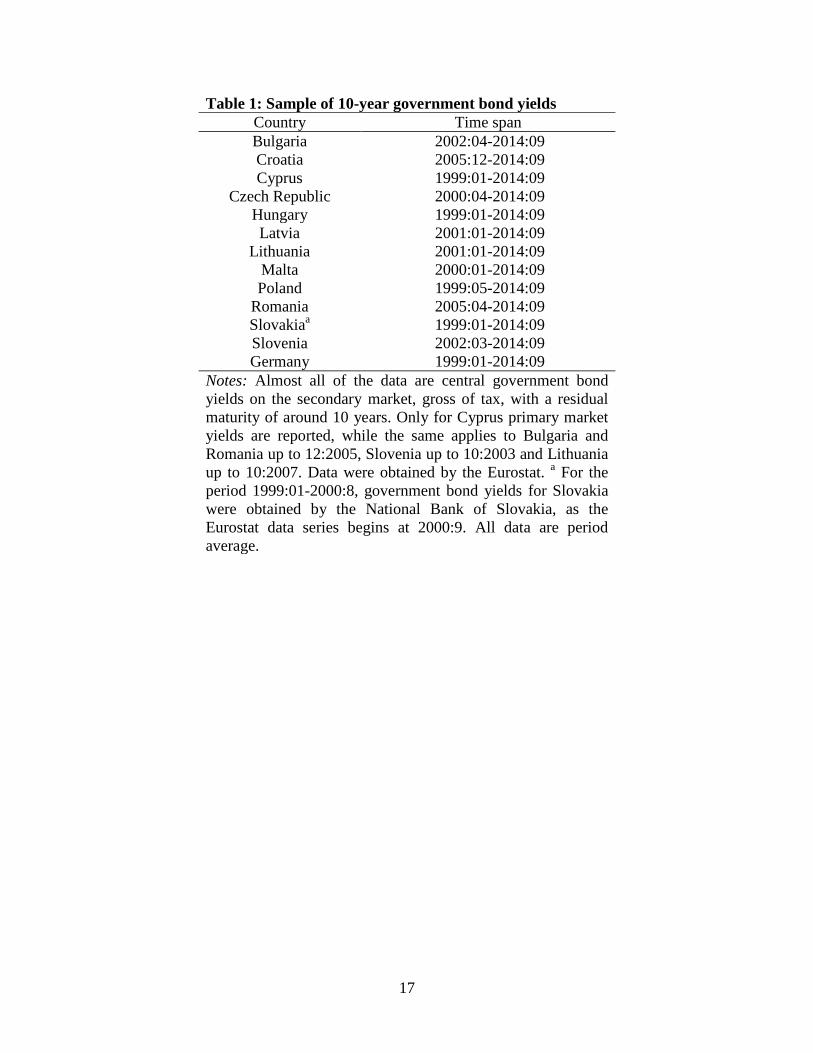
The data set consists of annualised monthly observations for 10-year government bond yields for

each new EU country and Germany. Estonia was left out of the analysis, because Estonian long-

term bonds are issued only occasionally and thus, their yields are not disseminated. The time

span for each country begins in 1999:01 with the establishment of the Eurozone, or later due to

data availability, and ends in 2014:09. The data details and their sources are reported in Table 1.

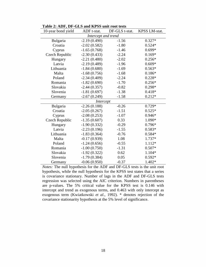
4.2 Unit Root Tests Results

Before testing for cointegration, each yield was tested for a unit root. Initially, the ADF, the DF-

GLS and the KPSS unit root tests were implemented. Columns 2 and 3 of table 2 report the

results for the ADF and the DF-GLS tests, respectively, which both indicate that the unit root

hypothesis cannot be rejected for any yield at the 5 per cent level of significance. The results for

10

the KPSS test are presented in the fourth column of table 2. Similarly, they provide evidence that

the null hypothesis of covariance stationarity is rejected for all yields.

4.3 Convergence of Monetary Policies

The possibility of monetary policy convergence between each new EU country and Germany is

examined by investigating long-run linkages in bond yields and testing for the restrictions

implied by the analysis of Section 2. Using two-dimensional VECMs for ( ), ,,t i t G ty r r= , each

consisting of the 10-year yields of the new EU country i and Germany, I firstly test for

cointegration between these two yields. If cointegration exists, then I test if the cointegrating

vector is ( )1, 1− . Secondly, conditional on the cointegrating vector being ( )1, 1− , I test for

cotrending and examine both strong and weak monetary policy convergence.

Before testing for cointegration, it is crucial to detect the structural breaks for the VECMs.

As suggested by economic theory and indicated by Koukouritakis (2013) the structural breaks

included in the VECMs had to be detected exogenously. This detection was based on specific

economic events that affected the sample countries. Hence for all VECMs, a single break is

allowed to be at the beginning of the current financial and debt crisis. According to the U.S.

National Bureau of Economic Research, the current financial crisis began in December 2007.

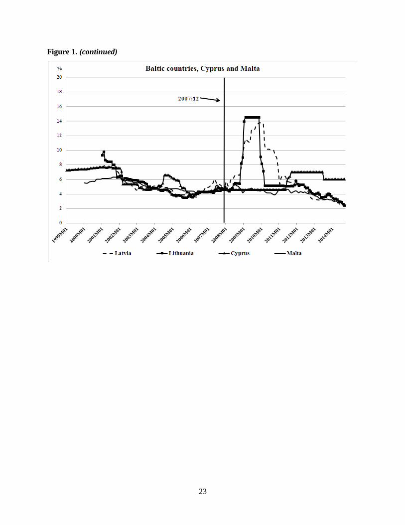
Figure 1 reports the yields for each sample country, along with the structural shift. One can easily

observe that from 2007 onwards, all yields show higher volatility, reflecting the fiscal deficit and

sovereign debt problems that several new EU countries faced.

4.3.1 Testing the cointegration hypothesis

To examine the hypothesis of cointegration, the model in equations (6) and (7) for each new EU

country and Germany was estimated. Then, for each country the LSTLR test statistic and the

corresponding response surface p-value were computed, using GAUSS codes.5 The lag length for

each VECM was selected using the Akaike information criterion (AIC). Also, the estimated

residuals in each VECM were checked for s-order serial correlation, using the multivariate

versions of the Lung-Box Q − tests and LM − tests. Under the null hypothesis of no serial

correlation in the error term of the VECM, these test statistics are asymptotically distributed as 5 The author is grateful to Carsten Trenkler for kindly providing him with the Gauss codes.

11

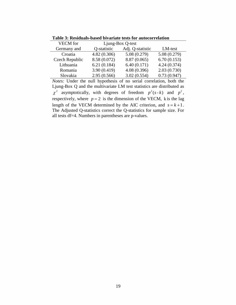
2χ with degrees of freedom 2 ( )p s k− and 2p , respectively (Johansen, 1995, p. 22). The

computed test statistics and associated p-values are reported in table 3. In all cases, both the Q

and LM tests do not reject the hypothesis of no serial correlation in the estimated residuals.

Table 4 reports the cointegration results. As shown in the third and fourth column, the

German 10-year bond yield is cointegrated only with the 10-year yields of Croatia, the Czech

Republic, Lithuania, Romania and Slovakia. In contrast, there is no evidence of cointegration

between the German 10-year yield and the 10-year yields of Bulgaria, Cyprus, Hungary, Latvia,

Malta, Poland and Slovenia. Next, for the five countries for which there is evidence of

cointegration, two separate tests were performed. Firstly, I tested the null hypothesis that the

German long rate is the shared common trend. The sixth column of table 4 gives the L-statistics

for specific choices of the matrix G . In particular, to test the null hypothesis that the German

long rate is the common trend, I set ( )0,1 'G = . As shown in this column, this null hypothesis is

not rejected in any case. Secondly, I tested the null hypothesis that the cointegrating vector

linking the pairs of 10-year bond yields is ( )1, 1− . Under the null hypothesis, this test is also

distributed asymptotically as 21χ (Johansen, 1995, p. 104). As shown in the seventh column of

table 4, this hypothesis is not rejected for all five countries. These results provide significant

empirical support for the necessary condition of monetary policy convergence of each of these

five countries to Germany. Alternatively, for these countries, Germany (as the dominant country

of the Eurozone) sets the long-term trend for expected inflation, and these five new EU countries

tend to adjust their monetary policies in order to achieve an expected inflation rate consistent

with that of Germany.

4.3.2 Testing the cotrending hypothesis and the significance of the constant term

As it was discussed in Section 2, interest rate or monetary policy convergence requires not only

that a pair of yields is cointegrated with cointegrating vector ( )1, 1− , but also that it is cotrending.

The latter means that yield spreads have no deterministic trends except possibly for a non-

negative constant term, including the level shifts where applicable. Furthermore, if the constant

term is insignificantly different from zero strong convergence has been achieved and the TEU

criterion is more than satisfied. Otherwise, if the constant term is significantly different from zero

12

but insignificantly different from 2%, then weak convergence has been achieved and the TEU

criterion for yields convergence is also satisfied.

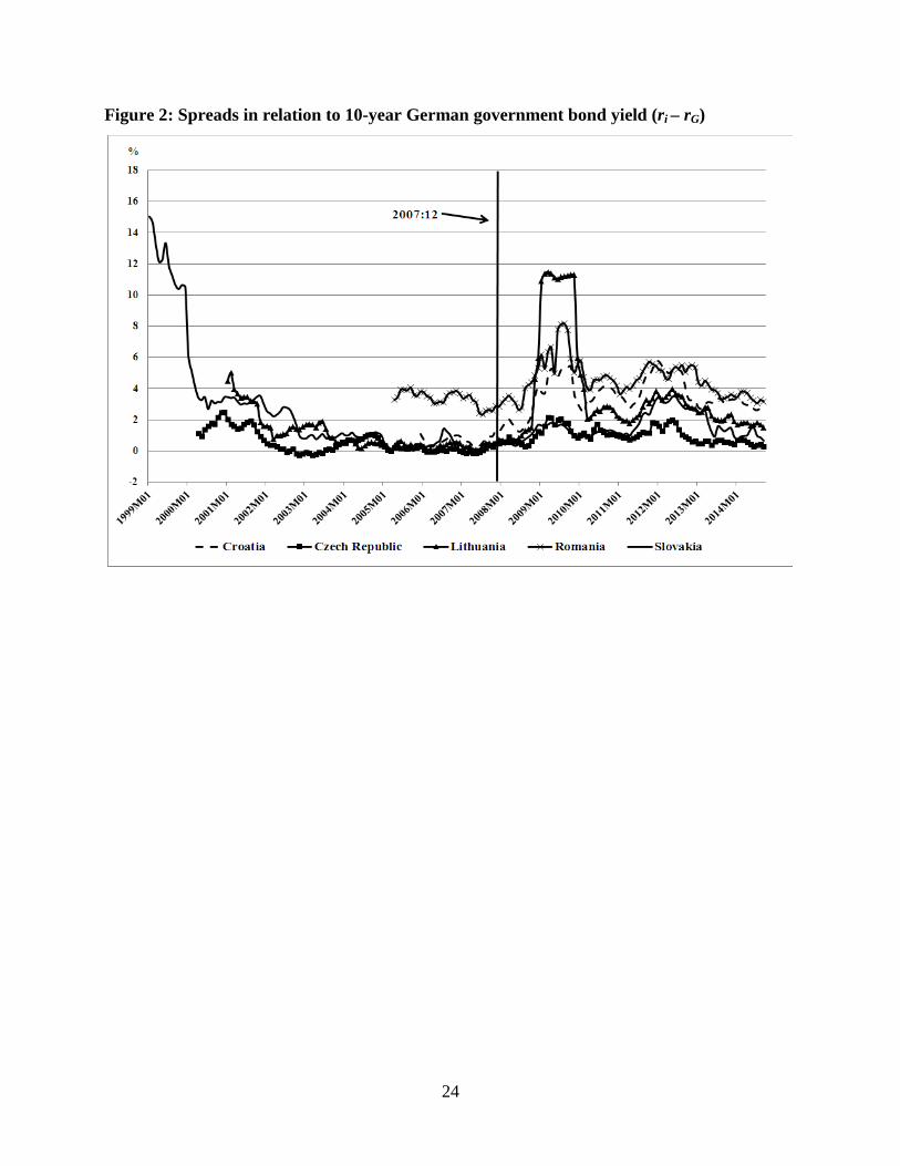
Figure 2 plots the yield spreads in relation to the 10-year German yield, for the five

countries that their yields are cointegrating with the German yield with cointegrating vector

( )1, 1− . These plots indicate different trending behaviour for these five countries. To test formally

for the significance of the trend and constant in each of these five spreads, I each yield spread

was regressed on an intercept, a linear trend and the respective level shift and trend shift, using

appropriate dummy variables. In each regression I included as many lags of the yield spread as

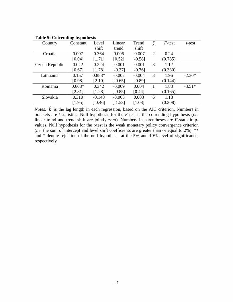
necessary, in order to make the residuals white noise. The results are reported in table 5. As

shown in the seventh column and based on a joint F-test, the cotrending hypothesis cannot be

rejected for any of the yield spreads of Croatia, the Czech Republic, Lithuania, Romania and

Slovakia. Consequently, these results provide strong statistical evidence of weak monetary policy

convergence between each of these five new EU countries and Germany, as far as deterministic

cotrending in the 10-year yield spreads is concerned.

Regarding the significance of the constant terms for each of the above five countries, as

shown in the second and third column of table 5, the intercept and the level shift of the yield

spreads of Croatia, the Czech Republic and Slovakia are statistically insignificant. Based on this

evidence, one can conclude that these three countries have achieved not only weak convergence,

but also strong monetary policy convergence, since the TEU criterion is more than satisfied. Note

that Germany plays a very important role in the economies of these three countries. For the

Romanian and Lithuanian yield spreads, for which there is also evidence of cotrending, the

intercept is significant for the former, while the level shift coefficient is significant for the latter.

Thus, in order to determine if Lithuania and Romania satisfy the weak monetary policy

convergence criterion, I performed an additional t-test on the sum of the intercept and the level

shift coefficient being greater than or equal to 2%, against the alternative of being less than 2%.

The respective t-statistics are reported in the eighth column of table 5 and indicate rejection of the

null hypothesis. Thus, there is evidence that also Lithuania and Romania satisfy the TEU

criterion for monetary policy convergence.

In the framework of the debt crisis in the Eurozone, the results reported in tables 4 and 5

indicate that even though Germany is the dominant country in the Eurozone and sets the

13

macroeconomic policies, seven new EU countries, namely Bulgaria, Cyprus, Hungary, Latvia,

Malta, Poland and Slovenia (regardless if they are members of the Eurozone or not) are unable to

follow them. Even though these new EU countries (a) managed to stabilise their exchange rates

during the last decade6, (b) adopted implicit or explicit inflation targeting polices in order to fight

inflation, (c) implemented tight fiscal policies in order to reduce fiscal deficit and public debts,

and (c) implemented structural reforms designed to support growth, the Eurozone debt crisis

harmed their economies significantly. Especially for Cyprus, Latvia and Slovenia, these results

do not necessarily imply monetary policy divergence with Germany. These countries are

Eurozone members and their monetary policies are no different from Germany's. Lack of yields’

convergence for these three countries can be attributed to the increased sovereign default risk due

to the Eurozone debt crisis, which in turn led to large and persistent risk premia. More

specifically, during the crisis period these countries suffered from recession. Latvia agreed with

the International Monetary Fund and the EU for rescue packages in 2008, while the credit ratings

of Cyprus and Slovenia downgraded in 2011 by the Credit Rating Agencies. Cyprus also suffered

a ‘haircut’ on deposits in 2013 due to the default of its commercial banks and in order to receive

bailout funds from the EU and the International Monetary Fund. It is also worth noting that the

credit ratings of the remaining new EU countries are at moderate risk. For Bulgaria, Hungary and

Poland, which are not yet Eurozone members, the evidence of yields’ divergence can be

attributed to differentials in expected inflation, as mentioned in section 2.

5. Concluding Remarks In this paper, 10-year bond yields convergence between each new EU country and Germany was

investigated. Because these bond yields are random walks with structural shifts over the sample

period, I evaluated these issues using cointegration and common trend techniques, in the presence

of structural breaks in the data.

The cointegration and cotrending analysis provides useful insights about the degree of

monetary policy convergence of the new EU countries to Germany (as the dominant country in

the Eurozone). Based on the analysis regarding long-term bond yields convergence, there is some

clear evidence of strong monetary convergence to Germany for Croatia, the Czech Republic and

6 Cyprus, Latvia, Malta and Slovenia joined the ERM II, Hungary pegged its currency to the euro, Poland implemented a free-floating exchange rate regime, while Bulgaria adopted a euro-based currency board.

14

Slovakia. Alternatively, under UIP and ex-ante relative PPP, the expected inflation rate of these

three countries has converged to the expected inflation rate of Germany. This is an expected

result because Germany plays a very important role especially in the economies of these three

countries. Furthermore, the results provide evidence of weak monetary convergence to Germany

for Lithuania and Romania. For the remaining seven new EU countries our evidence suggests

interest rate divergence and widening of the 10-year spread of these countries in relation to

Germany. At least for Cyprus, Latvia and Slovenia, this evidence can be attributed to the

increased sovereign default risk for these countries, which in turn led to large and persistent risk

premia.

Summarising, in the context of the debt crisis in the Eurozone, the empirical evidence

indicates that even though Germany as the dominant country, sets the macroeconomic policies in

the Eurozone, a lot of the new EU countries are unable to follow them. And this conclusion

addresses once more the issue of the core-periphery in the Eurozone and the future prospects of

it.

15

References Bernard, A.B. and Durlauf, S. (1995). ‘Convergence in International Output’, Journal of Applied

Econometrics, Vol 10, No. 2, pp. 97-108.

Bernard, A.B. and Durlauf, S. (1996). ‘Interpreting Tests of the Convergence Hypothesis’,

Journal of Econometrics, Vol. 71, No. 1-2, pp. 161-173.

Bhargava, A. (1986). ‘On the Theory of Testing for Unit Roots in Observed Time Series’,

Review of Economic Studies, Vol. 53, No. 3, pp. 369–384.

Camarero, M., Ordonez, J. and Tamarit, C.R. (2002). ‘Tests for Interest Rate Convergence and

Structural Breaks in the EMS: Further Analysis’, Applied Financial Economics, Vol. 12, No.

6, pp. 447-456.

Gonzalo, J. and Granger, C.W.J. (1995). ‘Estimation of Common Long-Memory Components in

Cointegrated Systems’, Journal of Business and Economics Statistics, Vol. 13, No. 1, pp. 27-

35.

Goodwin, B.K. and Grennes, T.J. (1994). ‘Real Interest Rate Equalization and Integration of

Financial Markets’, Journal of International Money and Finance, Vol. 13, No. 1, pp. 107-124.

Hafer, R.W. and Kutan, A.M. (1994). ‘A Long Run View of German Dominance and the Degree

of Policy Convergence in the EMS’, Economic Inquiry, Vol. 32, No. 4, pp. 684-695.

Haug, A.A., MacKinnon, J.G. and Michelis, L. (2000). ‘European Monetary Union: A

Cointegration Analysis’, Journal of International Money and Finance, Vol. 19, No. 3, pp. 419-

432.

Johansen, S. (1988). ‘Statistical Analysis of Cointegration Vectors’, Journal of Economic

Dynamics and Control, Vol. 12, No. 2-3, pp. 231-254.

Johansen, S. (1995). Likelihood-based Inference in Cointegrated Vector Autoregressive Models,

Oxford, Oxford University Press.

Karfakis, C.J. and Moschos, D.M. (1990). ‘Interest Rate Linkages within the European Monetary

System: A Time Series Analysis’, Journal of Money Credit and Banking, Vol. 22, No. 3, pp.

388-394.

Katsimbris, G.M. and Miller, S.M. (1993). ‘Interest Rate Linkages within the European Monetary

System: Further Analysis’, Journal of Money Credit and Banking, Vol. 25, No. 4, pp. 771-779.

16

Kirchgässner, G. and Wolters, J. (1995). ‘Interest Rate Linkages in Europe before and after the

Introduction of the European Monetary System’, Empirical Economics, Vol. 20, No. 3, pp.

435-454.

Koukouritakis, M. (2013). ‘Expectations Hypothesis in the Context of Debt Crisis: Evidence

from Five Major EU Countries’, Research in Economics, Vol. 67, No. 3, pp. 243-258.

Kwiatkowski, D., Phillips, P.C.B., Schmidt, P., Shin, Y. (1992). ‘Testing the Null Hypothesis of

Stationarity against the Alternative of a Unit Root’, Journal of Econometrics, Vol. 54, No. 1-3,

pp. 159-178.

Lütkepohl, H. and Saikkonen, P. (2000). ‘Testing for the Cointegrating Rank of a VAR Process

with a Time Trend’, Journal of Econometrics, Vol. 95, No. 1, pp. 177-198.

Mark, N. (1985). ‘Some Evidence on the International Inequality of Real Interest Rates’, Journal

of International Money and Finance, Vol. 4, No. 2, pp. 189-208.

Perron, P. (1997). ‘Further Evidence on Breaking Trend Functions in Macroeconomic Variables’,

Journal of Econometrics, Vol. 80, No. 2, pp. 355-385.

Perron, P. (2006). ‘Dealing with structural breaks’, in Patterson, K. and Mills T.C. (eds),

Palgrave Handbook of Econometrics, Vol. 1: Econometric Theory, New York: Palgrave

Macmillan, pp. 278-352.

Pesaran, M. (2007). ‘A Pair-Wise Approach to Testing for Output and Growth Convergence’,

Journal of Econometrics, Vol. 138, No. 1, pp. 312-355.

Saikkonen, P. and Lütkepohl, H. (2000). ‘Testing for the Cointegrating Rank of a VAR Process

with Structural Shifts’, Journal of Business and Economics Statistics, Vol. 18, No. 4, pp. 451-

464.

Schmidt, P. and Phillips, P.C.B. (1992). ‘LM Tests for a Unit Root in the Presence of

Deterministic Trends’, Oxford Bulletin of Economics and Statistics, Vol. 54, No. 3, pp. 257-

287.

Trenkler, C., Saikkonen, P. and Lütkepohl, H. (2008). ‘Testing for the Cointegrating Rank of a

VAR Process with Level Shift and Trend Break’, Journal of Time Series Analysis, Vol. 29,

No. 2, pp. 331-358.

17

Table 1: Sample of 10-year government bond yields Country Time span Bulgaria 2002:04-2014:09 Croatia 2005:12-2014:09 Cyprus 1999:01-2014:09

Czech Republic 2000:04-2014:09 Hungary 1999:01-2014:09 Latvia 2001:01-2014:09

Lithuania 2001:01-2014:09 Malta 2000:01-2014:09 Poland 1999:05-2014:09

Romania 2005:04-2014:09 Slovakiaa 1999:01-2014:09 Slovenia 2002:03-2014:09 Germany 1999:01-2014:09

Notes: Almost all of the data are central government bond yields on the secondary market, gross of tax, with a residual maturity of around 10 years. Only for Cyprus primary market yields are reported, while the same applies to Bulgaria and Romania up to 12:2005, Slovenia up to 10:2003 and Lithuania up to 10:2007. Data were obtained by the Eurostat. a For the period 1999:01-2000:8, government bond yields for Slovakia were obtained by the National Bank of Slovakia, as the Eurostat data series begins at 2000:9. All data are period average.

18

Table 2: ADF, DF-GLS and KPSS unit root tests 10-year bond yield ADF t-stat. DF-GLS t-stat. KPSS LM-stat.

Intercept and trend Bulgaria -2.19 (0.490) -1.56 0.327* Croatia -2.02 (0.582) -1.80 0.524* Cyprus -1.65 (0.768) -1.46 0.699*

Czech Republic -2.30 (0.433) -2.24 0.169* Hungary -2.21 (0.480) -2.02 0.256* Latvia -2.19 (0.489) -1.96 0.609*

Lithuania -1.84 (0.680) -1.69 0.563* Malta -1.68 (0.756) -1.68 0.186* Poland -2.34 (0.409) -2.24 0.228*

Romania -1.82 (0.690) -1.70 0.256* Slovakia -2.44 (0.357) -0.82 0.298* Slovenia -1.81 (0.697) -1.38 0.418* Germany -2.67 (0.249) -1.58 0.212*

Intercept Bulgaria -2.26 (0.188) -0.26 0.729* Croatia -2.05 (0.267) -1.51 0.525* Cyprus -2.08 (0.253) -1.07 0.946*

Czech Republic -1.35 (0.607) 0.33 1.090* Hungary -1.90 (0.332) -0.29 0.796* Latvia -2.23 (0.196) -1.55 0.583*

Lithuania -1.83 (0.364) -0.76 0.584* Malta -0.17 (0.939) 1.08 1.737* Poland -1.24 (0.656) -0.55 1.112*

Romania -1.00 (0.750) -1.31 0.507* Slovakia -1.92 (0.322) 0.62 1.104* Slovenia -1.79 (0.384) 0.05 0.592* Germany -0.06 (0.950) -0.37 1.402*

Notes: The null hypothesis for the ADF and DF-GLS tests is the unit root hypothesis, while the null hypothesis for the KPSS test states that a series is covariance stationary. Number of lags in the ADF and DF-GLS tests regression was selected using the AIC criterion. Numbers in parentheses are p-values. The 5% critical value for the KPSS test is 0.146 with intercept and trend as exogenous terms, and 0.463 with only intercept as exogenous term (Kwiatkowski et al., 1992). * denotes rejection of the covariance stationarity hypothesis at the 5% level of significance.

19

Table 3: Residuals-based bivariate tests for autocorrelation VECM for Ljung-Box Q-test

Germany and Q-statistic Adj. Q-statistic LM-test

Croatia 4.82 (0.306) 5.08 (0.279) 5.08 (0.279) Czech Republic 8.58 (0.072) 8.87 (0.065) 6.70 (0.153)

Lithuania 6.21 (0.184) 6.40 (0.171) 4.24 (0.374) Romania 3.90 (0.419) 4.08 (0.396) 2.03 (0.730) Slovakia 2.95 (0.566) 3.02 (0.554) 0.73 (0.947)

Notes: Under the null hypothesis of no serial correlation, both the Ljung-Box Q and the multivariate LM test statistics are distributed as

2χ asymptotically, with degrees of freedom 2 ( - )p s k and 2p , respectively, where 2p = is the dimension of the VECM, k is the lag length of the VECM determined by the AIC criterion, and 1s k= + . The Adjusted Q-statistics correct the Q-statistics for sample size. For all tests df=4. Numbers in parentheses are p-values.

20

Table 4: Cointegration and common trends tests results Germany with ( )0-p r

( )0LSTLR r p-values k L-statistic ( )1, -1 'CV =

Bulgaria 2 1

9.30 1.93

0.652 0.823

3 NA NA

Croatia 2 1

19.97** 1.06

0.031 0.903

5 2.64 (0.104)

2.04 (0.153)

Cyprus 2 1

11.13 2.21

0.472 0.768

3 NA NA

Czech Republic 2 1

17.22* 4.57

0.095 0.365

5 0.83 (0.363)

1.06 (0.303)

Hungary 2 1

10.19 3.51

0.563 0.528

3 NA NA

Latvia 2 1

8.48 2.28

0.733 0.761

12 NA NA

Lithuania 2 1

18.73* 1.76

0.059 0.852

4 1.00 (0.317)

1.00 (0.316)

Malta 2 1

10.29 1.57

0.554 0.881

3 NA NA

Poland 2 1

9.91 0.76

0.591 0.976

1 NA NA

Romania 2 1

21.74** 2.21

0.017 0.717

4 0.10 (0.756)

0.60 (0.440)

Slovakia 2 1

23.31** 0.60

0.011 0.986

4 2.27 (0.132)

0.05 (0.829)

Slovenia 2 1

8.62 0.81

0.719 0.973

3 NA NA

Notes: The value reported at the top of the second column for each panel is for

0 0r = , so that 0-p r p= is the dimension of the VECM. k is the estimated lag length in the VECM. The L-statistics are computed under the null hypothesis that the German 10-year bond yield is the common trend. Under the null hypothesis, the L-statistic is distributed as 2

1χ . Last column refers to the 0H that the cointegrating vector is ( )1, 1− . Under the null hypothesis, this test is also distributed as 2

1χ , asymptotically. Numbers in parentheses are p-values. ** and * denote rejection of the null hypothesis at the 5% and 10% level of significance, respectively. NA stands for “Not Applicable”.

21

Table 5: Cotrending hypothesis Country Constant Level

shift Linear trend

Trend shift

k F-test t-test

Croatia 0.007 [0.04]

0.364 [1.71]

0.006 [0.52]

-0.007 [-0.58]

2 0.24 (0.785)

Czech Republic 0.042 [0.67]

0.224 [1.78]

-0.001 [-0.27]

-0.001 [-0.76]

8 1.12 (0.330)

Lithuania 0.157 [0.98]

0.888* [2.10]

-0.002 [-0.65]

-0.004 [-0.89]

3 1.96 (0.144)

-2.30*

Romania 0.608* [2.31]

0.342 [1.28]

-0.009 [-0.85]

0.004 [0.44]

1 1.83 (0.165)

-3.51*

Slovakia 0.310 [1.95]

-0.148 [-0.46]

-0.003 [-1.53]

0.003 [1.08]

6 1.18 (0.308)

Notes: k is the lag length in each regression, based on the AIC criterion. Numbers in brackets are t-statistics. Null hypothesis for the F-test is the cotrending hypothesis (i.e. linear trend and trend shift are jointly zero). Numbers in parentheses are F-statistic p-values. Null hypothesis for the t-test is the weak monetary policy convergence criterion (i.e. the sum of intercept and level shift coefficients are greater than or equal to 2%). ** and * denote rejection of the null hypothesis at the 5% and 10% level of significance, respectively.

22

Figure 1. 10-year government bond yields

23

Figure 1. (continued)

24

Figure 2: Spreads in relation to 10-year German government bond yield (ri – rG)