interdecadal climate regime dynamics in the north pacific ocean: theories, observations and...

Progress in Oceanography 47 (2000) 355–379www.elsevier.com/locate/pocean

Interdecadal climate regime dynamics in theNorth Pacific Ocean: theories, observations and

ecosystem impacts

Arthur J. Miller *, Niklas SchneiderClimate Research Division, Scripps Institution of Oceanography, La Jolla, CA 92093-0224, USA

Abstract

Basin-scale variations in oceanic physical variables are thought to organize patterns of bio-logical response across the Pacific Ocean over decadal time scales. Different physical mech-anisms can be responsible for the diverse basin-scale patterns of sea-surface temperature (SST),mixed-layer depth, thermocline depth, and horizontal currents, although they are linked invarious ways. In light of various theories and observations, we interpret observed basinwidepatterns of decadal-scale variations in upper-ocean temperatures. Evidence so far indicates thatlarge-scale perturbations of the Aleutian Low generate temperature anomalies in the centraland eastern North Pacific through the combined action of net surface heat flux, turbulentmixing and Ekman advection. The surface-forced temperature anomalies in the central NorthPacific subduct and propagate southwestwards in the ocean thermocline to the subtropics butapparently do not reach the equator. The large-scale Ekman pumping resulting from changesof the Aleutian Low forces western-intensified thermocline depth anomalies that are approxi-mately consistent with Sverdrup theory. These thermocline changes are associated with SSTanomalies in the Kuroshio/Oyashio Extension that are of the same sign as those in the centralNorth Pacific, but lagged by several years. The physics of the possible feedback from the SSTanomalies to the Aleutian Low, which might close a coupled ocean–atmosphere mode of deca-dal variability, is poorly understood and is an area of active research. The possible responsesof North Pacific Ocean ecosystems to these complicated physical patterns is summarized.2000 Elsevier Science Ltd. All rights reserved.

* Corresponding author.E-mail address:[email protected] (A.J. Miller).

0079-6611/00/$ - see front matter 2000 Elsevier Science Ltd. All rights reserved.PII: S0079 -6611(00 )00044-6

356 A.J. Miller, N. Schneider / Progress in Oceanography 47 (2000) 355–379

Contents

1. Introduction . . . . . . . . . . . . . . . . . . . . . . . . . . . . . . . . . . . . . . . . . . 356

2. Theoretical arguments of North Pacific decadal variations . . . . . . . . . . . . . . 3572.1. Stochastic atmospheric forcing . . . . . . . . . . . . . . . . . . . . . . . . . . . . . 3572.2. Atmospheric teleconnections to the North Pacific . . . . . . . . . . . . . . . . . . 3582.3. Midlatitude ocean–atmosphere interactions . . . . . . . . . . . . . . . . . . . . . . 3622.4. Tropical–extratropical interactions . . . . . . . . . . . . . . . . . . . . . . . . . . . 3642.5. Oceanic teleconnections to the midlatitudes . . . . . . . . . . . . . . . . . . . . . 3682.6. Intrinsic ocean variability . . . . . . . . . . . . . . . . . . . . . . . . . . . . . . . . 369

3. Biological impacts . . . . . . . . . . . . . . . . . . . . . . . . . . . . . . . . . . . . . . 369

4. Summary . . . . . . . . . . . . . . . . . . . . . . . . . . . . . . . . . . . . . . . . . . . . 372

Acknowledgements . . . . . . . . . . . . . . . . . . . . . . . . . . . . . . . . . . . . . . . . . . 373

References . . . . . . . . . . . . . . . . . . . . . . . . . . . . . . . . . . . . . . . . . . . . . . . 373

1. Introduction

Variations of oceanic physical variables are clearly involved in many aspects ofthe variability of biological populations on seasonal and interannual timescales. Butthere is great uncertainty of the mechanisms by which decadal variations of physicalvariables influence biological populations (e.g., Beamish & McFarlane, 1989; Beam-ish, 1995; Holloway & Muller, 1998). While physical variables are known to changeon decadal timescales, their preferred frequencies, their characteristic patterns andtheir relative temporal phasing are still being sorted out. In order to determine theinfluence of physical ocean climate variations on North Pacific biological populationsbetter, it is useful to outline what processes are likely to control these variations ondecadal timescales.

The decadal variations in the physics can take the form of gradual drifts, smoothoscillations or step-like shifts such as those of 1976–77 (Ebbesmeyer, Cayan,McLain, Nichols, Peterson & Redmond, 1991; Trenberth & Hurrell, 1994; Miller,Cayan, Barnett, Graham & Oberhuber, 1994b; Wu & Hsieh, 1999) and of 1989(Hare & Mantua, 2000). Many theories have recently been proposed to explain thedecadal variations of the midlatitude North Pacific Ocean (e.g., see the recent reviewby Latif, 1998), often predicting oscillatory behavior in the presence of a stochasticcomponent. Related observational studies have sought to uncover the characteristicsignatures of these decadal variations, but the temporally and spatially limited obser-vations preclude definitive characterizations of oscillatory, step-like or randombehavior.

The biological variability may not linearly mimic the decadal variations in thephysical forcing. Attention is often focussed on identifying whether or not a ‘regime

357A.J. Miller, N. Schneider / Progress in Oceanography 47 (2000) 355–379

shift’ has occurred, that is, a change from a persistent and relatively stable periodof biological productivity that accompanies a change after a similarly stable periodin physical oceanographic variables. Our presently imprecise understanding of thephysical mechanisms of decadal variations and the even greater obscurity of thebiological response mechanisms, makes it difficult to define ‘regime’ precisely.Nonetheless, statistical techniques designed to detect step-like behavior may provideuseful regime-change indicators. Examples include interversion analysis (Hare &Francis, 1995), interfering patterns of two or more decadal-scale periodicities(Minobe, 1999), and compositing techniques that posit step functions (Ebbesmeyeret al., 1991; Hare & Mantua, 2000). However, the presently limited observationscannot be used to discriminate confidently oscillatory from step-like models. For thepurposes of this paper, any physical or biological state that persists over decadaltimescales is considered to exhibit ‘regime-like’ characteristics.

Our first task here is to determine the consistency between oceanic observationsand the physical processes of the various theoretical models for North Pacific decadalvariability. Our second task is to summarize the proposed linkages between thesephysical processes and decadal changes in North Pacific oceanic ecosystems. Overallwe hope that this discussion will aid in reconciling many aspects of the observationsand theories of oceanic physical decadal variations and their consequent impacton biology.

2. Theoretical arguments of North Pacific decadal variations

2.1. Stochastic atmospheric forcing

The simplest theories suggest that stochastic variations in atmospheric forcing(e.g., James & James, 1989) drive the long-term ocean variations. This concept wasfirst proposed by Hasselmann (1976) and Frankignoul and Hasselmann (1977) as athermodynamic explanation of low-frequency sea-surface temperature (SST,hereinafter) anomaly variations. A white-noise surface heat flux forcing results in ared SST spectrum, the details of which are controlled by a feedback parameter thatby balancing the random forcing at low frequencies limits the variance.

This idea has recently extended in two directions. Firstly, Barsugli and Battisti(1998) incorporated air temperature as an additional variable to explore better thelocal feedback processes. Their model provides an important interpretative tool forunderstanding the influences of specified SST anomaly experiments in atmosphericgeneral circulation model hindcasts. Their model shows that midlatitude ocean–atmosphere coupling increases the variability in and decreases the energy fluxbetween the atmosphere and the ocean. Second, Frankignoul, Mu¨ller and Zorita(1997) treated the dynamic problem of ocean currents driven stochastically by windstress curl on decadal time scales, and showed that the resulting ocean velocity spec-tral levels are comparable to those of observations.

Stochastic models can also explain decadal-scale spectral peaks without invokingocean–atmosphere feedback. For example, Saravanan and McWilliams (1998)


proposed an advective resonance that postulates a preferred atmospheric spatialpattern (necessarily having at least one zero crossing in the ocean basin) and whitenoise atmospheric forcing in time (cf. Tsonis, Roebber & Elsner, 1999). If meanoceanic currents produce a preferred direction for the phase propagation of theoceanic response, a spectral peak can occur in the oceanic response withoutocean–atmosphere feedback. Neelin and Weng (1999) propose that a similar stochas-tic resonance happens if oceanic waves provide the preferred direction of propagatingoceanic response. Note that Jin (1997) and Frankignoul et al. (1997) outlined thisuncoupled resonance effect in their earlier work.

The striking comparability of the spectral shapes and levels predicted by stochastictheories with observations give a zeroth order view of the way the North Pacificocean behaves on decadal time scales. Temporal spectra of various observed oceanicvariables are generally red but also exhibit weak spectral peaks at decadal timescales(e.g., Mann & Park, 1996). However, it remains unclear if these peaks are associatedwith random processes or the preferred frequencies of coupled modes of variability(e.g., Wunsch, 1999). The observed characteristic spatial patterns (Fig. 1) seen inSST (e.g., Tanimoto, Iwasaka, Hanawa & Toba, 1992) or in the thermocline (Miller,Cayan & White, 1998; Tourre, White & Kushnir (1999)) also may be indicative ofpreferred natural modes in the oceanic response or simply a passive response to theatmospheric forcing functions.

2.2. Atmospheric teleconnections to the North Pacific

Effects external to the midlatitude North Pacific may also directly force part ofits decadal variability. For example, if there are decadal oscillations intrinsic to thetropical Pacific, they are likely to teleconnect to the midlatitudes (Bjerknes, 1966;Alexander, 1992; Lau, 1997) and produce decadal variations there which resemblethe interannual patterns associated with El Nin˜o (e.g., Zhang, Wallace & Battisti,1997; Zhang, Sheng & Shabbar, 1998b). Such a teleconnection process was invokedby Trenberth (1990), Graham (1994) and Graham, Barnett, Wilde, Ponater and Schu-bert (1994) to explain aspects of the 1976–77 climate shift in the North Pacific(Trenberth & Hurrell, 1994). Indeed, some coupled models are found to be capableof generating decadal oscillations intrinsic to the tropics (e.g., Tziperman, Cane &Zebiak, 1995; Yukimoto et al., 1996; Knutson & Manabe, 1998; Schneider, 2000)these may teleconnect through the atmosphere to the midlatitudes forcing changesin SST and ocean currents.

This atmospheric teleconnection view was supported by Miller, Cayan, Barnett,Graham and Oberhuber (1994a) and Miller et al. (1994b) who showed that the mod-eled SST pattern associated with the 1976–77 shift can be viewed as a response tolocal surface forcing by the atmosphere without ocean feedback. As the AleutianLow strengthens and westerly winds increase in the central North Pacific, the SSTcools in response to enhanced surface heat–flux cooling, southward Ekman currentadvection of cool SST and increased turbulent mixing of underlying cooler water.In the eastern North Pacific, SST warms because the strengthened Aleutian Lowresults in increased southerly winds which are warmer and moister than normal and


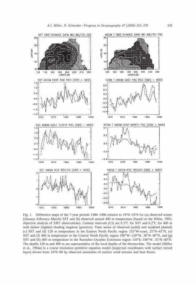
Fig. 1. Difference maps of the 7-year periods 1980–1986 relative to 1970–1976 for (a) observed winter(January–February–March) SST and (b) observed annual 400 m temperature (based on the White, 1995,objective analysis of XBT observations). Contour intervals (CI) are 0.3°C for SST and 0.2°C for 400 mwith darker (lighter) shading negative (positive). Time series of observed (solid) and modeled (dotted)(c) SST and (d) 120 m temperature in the Eastern North Pacific region 135°W-coast, 25°N–45°N, (e)SST and (f) 400 m temperature in the Central North Pacific region 180°W–150°W, 30°N–40°N, and (g)SST and (h) 400 m temperature in the Kuroshio–Oyashio Extension region 150°E–180°W, 35°N–40°N.The depths 120 m and 400 m are representative of the local depths of the thermocline. The model (Milleret al., 1994a) is a coarse resolution primitive equation model (isopycnal coordinates with surface mixedlayer) driven from 1970–88 by observed anomalies of surface wind stresses and heat fluxes.


hence reduce surface heat loss (Cayan, Miller, Barnett, Graham, Ritchie & Ober-huber, 1995). The southerly winds during the 1976–77 winter also resulted in east-ward Ekman currents that advected warmer open ocean SST towards the climatolog-ically cooler region near the coast. During other time intervals, however, variationsin horizontal advection and mixing are usually much smaller than the dominant heat–flux forcing in the eastern North Pacific. This SST pattern, with opposite polarity inthe central and eastern North Pacific (Fig. 1a), occurs so commonly on seasonal,interannual and decadal timescales (Tanimoto et al., 1992) that we refer to it belowas the ‘canonical SST pattern’.

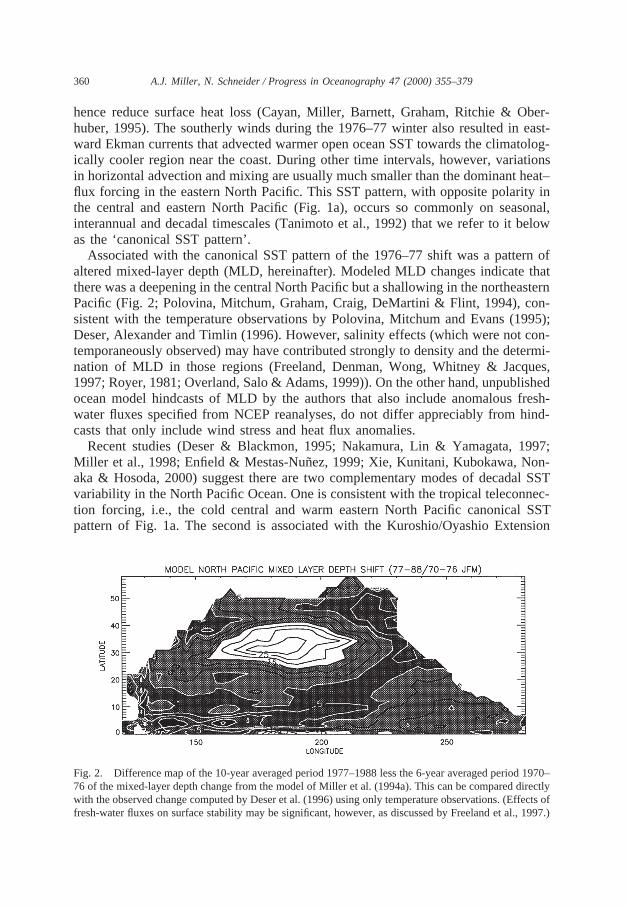
Associated with the canonical SST pattern of the 1976–77 shift was a pattern ofaltered mixed-layer depth (MLD, hereinafter). Modeled MLD changes indicate thatthere was a deepening in the central North Pacific but a shallowing in the northeasternPacific (Fig. 2; Polovina, Mitchum, Graham, Craig, DeMartini & Flint, 1994), con-sistent with the temperature observations by Polovina, Mitchum and Evans (1995);Deser, Alexander and Timlin (1996). However, salinity effects (which were not con-temporaneously observed) may have contributed strongly to density and the determi-nation of MLD in those regions (Freeland, Denman, Wong, Whitney & Jacques,1997; Royer, 1981; Overland, Salo & Adams, 1999)). On the other hand, unpublishedocean model hindcasts of MLD by the authors that also include anomalous fresh-water fluxes specified from NCEP reanalyses, do not differ appreciably from hind-casts that only include wind stress and heat flux anomalies.

Recent studies (Deser & Blackmon, 1995; Nakamura, Lin & Yamagata, 1997;Miller et al., 1998; Enfield & Mestas-Nun˜ez, 1999; Xie, Kunitani, Kubokawa, Non-aka & Hosoda, 2000) suggest there are two complementary modes of decadal SSTvariability in the North Pacific Ocean. One is consistent with the tropical teleconnec-tion forcing, i.e., the cold central and warm eastern North Pacific canonical SSTpattern of Fig. 1a. The second is associated with the Kuroshio/Oyashio Extension

Fig. 2. Difference map of the 10-year averaged period 1977–1988 less the 6-year averaged period 1970–76 of the mixed-layer depth change from the model of Miller et al. (1994a). This can be compared directlywith the observed change computed by Deser et al. (1996) using only temperature observations. (Effects offresh-water fluxes on surface stability may be significant, however, as discussed by Freeland et al., 1997.)


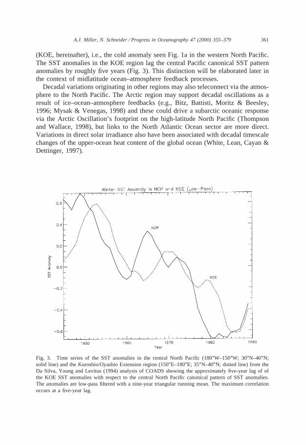
(KOE, hereinafter), i.e., the cold anomaly seen Fig. 1a in the western North Pacific.The SST anomalies in the KOE region lag the central Pacific canonical SST patternanomalies by roughly five years (Fig. 3). This distinction will be elaborated later inthe context of midlatitude ocean–atmosphere feedback processes.

Decadal variations originating in other regions may also teleconnect via the atmos-phere to the North Pacific. The Arctic region may support decadal oscillations as aresult of ice–ocean–atmosphere feedbacks (e.g., Bitz, Battisti, Moritz & Beesley,1996; Mysak & Venegas, 1998) and these could drive a subarctic oceanic responsevia the Arctic Oscillation’s footprint on the high-latitude North Pacific (Thompsonand Wallace, 1998), but links to the North Atlantic Ocean sector are more direct.Variations in direct solar irradiance also have been associated with decadal timescalechanges of the upper-ocean heat content of the global ocean (White, Lean, Cayan &Dettinger, 1997).

Fig. 3. Time series of the SST anomalies in the central North Pacific (180°W–150°W; 30°N–40°N;solid line) and the Kuroshio/Oyashio Extension region (150°E–180°E; 35°N–40°N; dotted line) from theDa Silva, Young and Levitus (1994) analysis of COADS showing the approximately five-year lag of ofthe KOE SST anomalies with respect to the central North Pacific canonical pattern of SST anomalies.The anomalies are low-pass filtered with a nine-year triangular running mean. The maximum correlationoccurs at a five-year lag.


2.3. Midlatitude ocean–atmosphere interactions

On sufficiently long time scales significant thermal feedback from the midlatitudeocean to the overlying atmosphere must occur. However, the strength of the midlati-tude ocean-to-atmosphere feedbacks as a function of time scale is unknown. Severalmodels have suggested these feedbacks are important on decadal timescales.

Latif and Barnett (1994, 1996) proposed a midlatitude ocean–atmosphere feedbackmechanism to explain a coupled ocean–atmosphere model that exhibits oscillationswith roughly 20-year period. They interpreted that oscillation as follows. An initial,say, cold SST anomaly in the Kuroshio Extension grows via some ocean–atmospherefeedback process (e.g., Palmer & Sun, 1985; Miller, 1992). The atmospheric pressurepattern excited during this feedback process is associated with wind-stress curlchanges (Ekman pumping) which force Rossby waves. These Rossby waves arriveat the western boundary many years later and subsequently enhance the polewardtransport of the subtropical gyre western boundary current. This enhances the heattransport into the Kuroshio Extension, eventually reversing the sign of the originallycold SST anomaly. Robertson (1996) showed that a subtropical gyre advective effectthat is balanced by surface heat fluxes into the atmosphere leads to decadal variationsin another coupled model.

Simpler versions of this type of feedback mechanism have been analyzed by manyauthors (Jin, 1997; Xu, Barnett & Latif, 1998; Goodman & Marshall, 1998; Talley,1999; Neelin & Weng, 1999; Mu¨nnich, Latif, Venzke & Maier-Reimer, 1998; Watan-abe & Kimoto, 2000). These simpler models usually rely on two questionableapproximations: specifying direct relationships between thermocline depth and SSTanomalies, which is not generally valid in midlatitudes; and between SST anomaliesand the overlying atmospheric response, the mechanisms for which are still unclear(e.g., Lau, 1997). Cessi (2000), on the other hand, derives a consistent approximationfor the non-linear effects of synoptic-scale variability of the atmosphere in her modelthat exhibits decadal oscillations as a result of gyre-scale processes affecting oceanicheat transport and SST. These theoretical models allow a simple and quantitativeestimation of possible feedbacks loops in the midlatitude system. They suggest thatthe thermocline adjustment process (especially its time-lagged response) is essentialto determining the period of oscillations and that the strength and nature of theocean-to-atmosphere feedback is central in determining whether oscillations are self-sustaining or exponentially damped.

The observed subsurface temperature fluctuations (e.g., Fig. 1b) indeed exhibit awestward intensified structure in the KOE region of the subpolar gyre consistentwith Sverdrup-like dynamics resulting from an increase in wind stress curl forcingfrom the 1970s to the 1980s. Miller et al. (1998) separated the decadal anomalies ofsubsurface temperature from the westward propagating ENSO-time scale anomalies(Miller, White & Cayan, 1997) in the North Pacific for the time period 1970–88.They then compared the observations to decadal temperature anomalies from anumerical hindcast forced by observed heat flux and wind stress anomalies. Themodel physics indeed show that wind stress curl drives the model vorticity equationyielding simulated thermocline variations similar to those observed (Fig. 1d,f,h).


Deser, Alexander and Timlin (1999) directly computed decadal changes in the zonalgeostrophic current in the KOE using the subsurface temperature dataset. Theyshowed KOE currents are consistent with wind stress curl forcing the ocean gyrebut with a 4–5 year phase lag in the response of KOE currents. These complementaryresults give a directly observed basin-scale perspective to the previous studies ofobserved changes in western boundary current transport and inferences of transportchanges deduced from wind stress curl (Sekine, 1988; Trenberth, 1991; Tabata, 1991;Qiu & Joyce, 1992; Watanabe & Mizuno, 1994; Hanawa, 1995; Lagerloef, 1995;Yasuda & Hanawa, 1997; Schwing, 1998).

An interesting aspect of these results is that the westward intensified thermoclinechanges are nearly stationary without any obvious propagating component. As theAleutian Low wind stress curl changes on the 20-year time scale, the subpolar gyreadjusts in place with no evident westward phase propagation associated with Rossbywaves which ubiquitously provide the delayed response in the simple coupled mod-els. The subtropical gyre behaves similarly with a stationary response to overlyingwind stress curl variations which lags the subpolar wind stress curl forcing by severalyears (Tourre et al., 1999; Miller et al., 1998). An additional oceanic signal thatdoes propagate gives the appearance of linking the stationary western-intensifiedsubpolar and subtropical gyre responses, but that signal is associated with anomaloussubduction (to be discussed next) and thus has different physics than the adiabaticallyforced thermocline adjustment. The combination of these results is the appearanceof a circumbasin transit of temperature anomalies, interpreted by Zhang and Levitus(1997) as an advective process (mean circulation advecting subsurface temperatureanomalies). But that advection process only appears to be occurring over a shortpath (Schneider et al., 1999b), while the rest of the signal is wind-stress curl forced.

Returning to the oceanic surface response, the SST in the KOE region decreasesapproximately five years after the 1976–77 shift cooling of the the central NorthPacific canonical SST pattern (Deser et al., 1996; Miller et al., 1998) as shown inFig. 3. This is in contrast to the Latif–Barnett scenario that calls for warming in theKOE region after cooling in the central North Pacific. The cooling in the KOE isclearly associated with the gyre-scale response to wind-stress curl forcing, but it isunclear whether this KOE SST pattern results from changes in thermal structure atthe base of the mixed layer, from anomalous advection by geostrophic or Ekmancurrents or from yet another process.

It is interesting to speculate on a possible feedback loop that differs from theLatif–Barnett interpretation as follows. An anomalously strong Aleutian Low initiallyforces the canonical pattern with cold central North Pacific SST as described inSection 2.2 above. This is associated with increased Ekman upwelling over the sub-polar gyre and increased Ekman downwelling over the subtropical gyre, spinning upboth gyres and their western boundary currents. If the heat transport of the subtropicalgyre dominates, the KOE SST should warm after a few years. But this is not observed(Fig. 3). If heat transport by the subpolar gyre dominates, the KOE SST should coolafter a few years, as is observed (Fig. 3). Preliminary analyses by the authors of thecoupled model that contains the Latif–Barnett mode (Barnett, Pierce, Saravanan,Schneider, Dommenget & Latif, 1999) show that the canonical SST pattern leads


the like-signed KOE SST by roughly five years as in Fig. 3. The subpolar maytherefore be more important than the subtropical gyre in the observed decadal vari-ation associated with the 1976–77 shift (Miller et al., 1998).

The feedbacks associated with midlatitude SST anomalies are uncertain (Lau, 1997).However, SST anomalies in the KOE region, rather than in the central North Pacific,have recently been associated with generating a significant atmospheric response thatdepends sensitively on the background state (e.g., Peng, Robinson & Hoerling, 1997).Continuing our speculation on the decadal feedback loop, if the cool SST in the KOEleads to a strengthened Aleutian Low (as in the equivalent barotropic response of thePalmer & Sun, 1985 model) a positive feedback results and persistent states may beestablished. If the cool SST in the KOE leads to a weakened Aleutian Low, a negativefeedback results and decadal oscillations may follow.

If the cool SST in the KOE leads to a regional atmospheric response that doesnot influence the Aleutian Low, the feedback loop does not close. In that case, spec-tral peaks can only result from stochastic resonances (e.g., Neelin & Weng, 1999).However, Pierce et al. (personal communication) argue against such an explanationfor the 20-year spectral peak in the Latif–Barnett coupled model. They show thatthe time sequence of the surface forcing is critical to existence of the peak sincerandomizing the monthly mean forcing of an ocean-only hindcast of the coupledmodel run causes the disappearance of the 20-year peak in the KOE. These resultssuggest a decadal feedback is indeed operating in the coupled model. In summary,the sensitivity of the atmosphere to KOE SST is clearly the key issue to determiningwhether natural decadal variability can be explained by deterministic midlatitudecoupled modes or as a stochastic response (as in Section 2.1).

2.4. Tropical–extratropical interactions

Different ideas to explain midlatitude decadal variations involve tropical–extra-tropical interaction. Gu and Philander (1997) proposed a mechanism whereby atmos-pheric teleconnections from, say, warm tropical SST drive cool anomalous SST inthe central North Pacific or South Pacific; this changes the temperature of water thatis subducted into the thermocline and follows the mean circulation to the tropics.Once the anomalously cool subducted water reaches the tropical strip many yearslater it is presumed to upwell to the surface and cause the SST to cool along theequator resulting in oppositely signed teleconnection patterns.

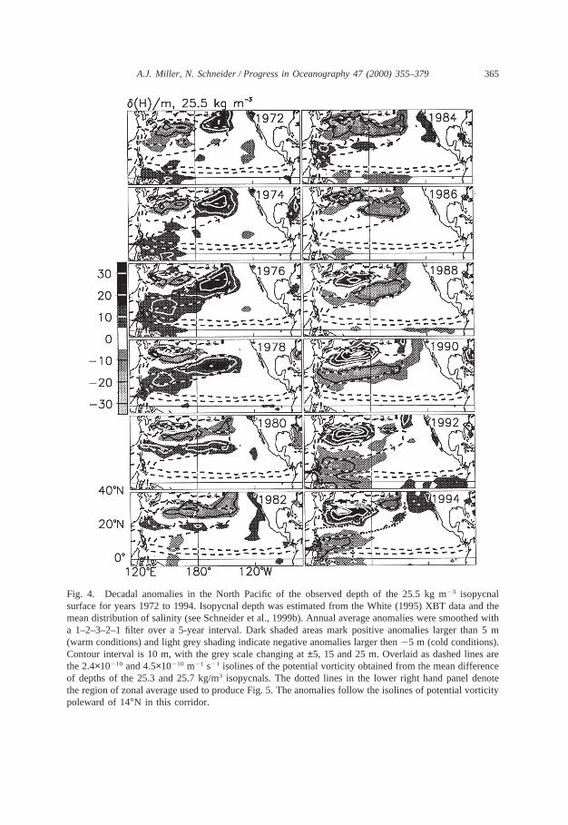
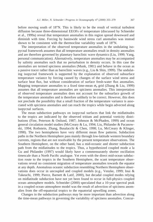
The Gu–Philander mechanism was motivated by the analysis of Deser et al. (1996)who showed a vertical section of temperature anomalies in the North Pacific thatmigrate southward and downward. Schneider, Miller, Alexander and Deser (1999a)studied the same dataset (White, 1995) and examined the full three-dimensionalstructure of these anomalies using isotherm displacements as a surrogate for tempera-ture. To determine if thermal anomalies can be better followed to the equator usingisopycnals rather than isotherm displacements, Fig. 4 displays this subduction processby showing the anomalous depths of thesq=25.5 surface estimated from time-depen-dent temperature and time-averaged salinity observations. The results are consistentwith the isothermal framework of Schneider et al. (1999a), simple Sverdrup theory,


Fig. 4. Decadal anomalies in the North Pacific of the observed depth of the 25.5 kg m23 isopycnalsurface for years 1972 to 1994. Isopycnal depth was estimated from the White (1995) XBT data and themean distribution of salinity (see Schneider et al., 1999b). Annual average anomalies were smoothed witha 1–2–3–2–1 filter over a 5-year interval. Dark shaded areas mark positive anomalies larger than 5 m(warm conditions) and light grey shading indicate negative anomalies larger then25 m (cold conditions).Contour interval is 10 m, with the grey scale changing at±5, 15 and 25 m. Overlaid as dashed lines arethe 2.4×10210 and 4.5×10210 m21 s21 isolines of the potential vorticity obtained from the mean differenceof depths of the 25.3 and 25.7 kg/m3 isopycnals. The dotted lines in the lower right hand panel denotethe region of zonal average used to produce Fig. 5. The anomalies follow the isolines of potential vorticitypoleward of 14°N in this corridor.


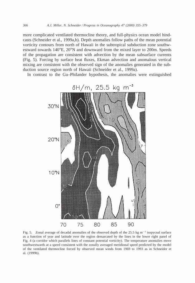
more complicated ventilated thermocline theory, and full-physics ocean model hind-casts (Schneider et al., 1999a,b). Depth anomalies follow paths of the mean potentialvorticity contours from north of Hawaii in the subtropical subduction zone southw-estward towards 140°E, 20°N and downward from the mixed layer to 200m. Speedsof the propagation are consistent with advection by the mean subsurface currents(Fig. 5). Forcing by surface heat fluxes, Ekman advection and anomalous verticalmixing are consistent with the observed sign of the anomalies generated in the sub-duction source region north of Hawaii (Schneider et al., 1999a).

In contrast to the Gu–Philander hypothesis, the anomalies were extinguished

Fig. 5. Zonal average of decadal anomalies of the observed depth of the 25.5 kg m23 isopycnal surfaceas a function of year and latitude over the region demarcated by the lines in the lower right panel ofFig. 4 (a corridor which parallels lines of constant potential vorticity). The temperature anomalies movesouthwestwards at a speed consistent with the zonally averaged meridional speed predicted by the modelof the ventilated thermocline forced by observed mean winds from 1969 to 1993 as in Schneider etal. (1999b).


before moving south of 18°N. This is likely to be the result of vertical turbulentdiffusion because three-dimensional EEOFs of temperature (discussed by Schneideret al., 1999a) reveal that temperature anomalies in this region spread downward anddiminish with time. Forcing by basinwide wind stress curl anomalies was insteadshown to be consistent with the thermocline variability south of 18°N.

The interpretation of the observed temperature anomalies in the undulating iso-pycnal framework assumes that all temperature anomalies result in density anomaliesand are therefore governed by planetary baroclinic wave dynamics (Liu, 1999; Yang,personal communication). Alternatively, temperature anomalies may be accompaniedby salinity anomalies such that no perturbation in density occurs. In this case theanomalies are termed spiciness anomalies (Munk, 1981) and behave in the ocean asa passive tracer rather than as baroclinic waves (e.g., Liu & Shin, 1999). The undulat-ing isopycnal framework is supported by the explanation of observed subsurfacetemperature variance by forcing caused by changes of the surface wind stress andsurface heat flux, but without consideration of surface fresh-water flux anomalies.Mapping temperature anomalies to a fixed time-meansq grid (Zhang & Liu, 1999)assumes that all temperature anomalies are spiciness anomalies. This interpretationof observed temperature anomalies does not account for the subsurface growth ofthe temperature anomalies and is therefore unlikely to be correct. However, this doesnot preclude the possibility that a small fraction of the temperature variance is asso-ciated with spiciness anomalies and can reach the tropics while begin advected alongisopycnal surfaces.

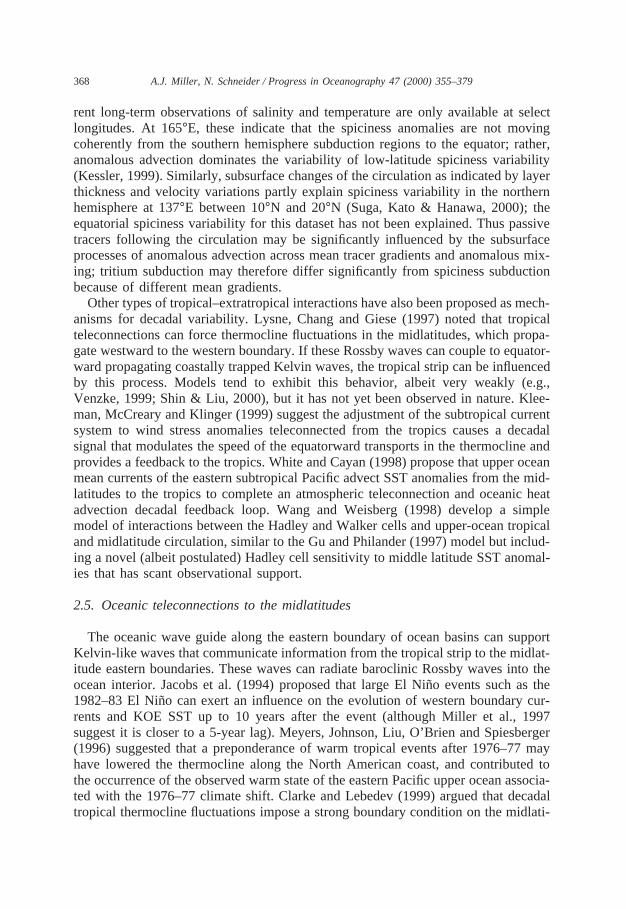
The mean subduction pathways on isopycnal surfaces that link the midlatitudesto the tropics are indicated by the observed tritium and potential vorticity distri-butions (Fine, Peterson & Ostlund, 1987; Johnson & McPhaden, 1999) and oceangeneral circulation model studies (McCreary & Lu, 1994; Liu, Philander & Pacanow-ski, 1994; Rothstein, Zhang, Busalacchi & Chen, 1998; Lu, McCreary & Klinger,1998). The two hemispheres have very different mean flow patterns. Subductionpaths in the Northern Hemisphere pass mainly through low-latitude western boundarycurrents, regions that are not resolvable by the present temperature observations. TheSouthern Hemisphere, on the other hand, has a mid-oceanic and shorter subductionpath from the midlatitudes to the tropics. Thus, a hypothesized coupled mode a laGu and Philander (1997) would likely have a commensurately shorter oscillationtimescale than a North Pacific analogue. Yet even with the direct mid-ocean subduc-tion route to the tropics in the Southern Hemisphere, the scant temperature obser-vations reveal no consistent migration of temperature anomalies towards the equatorat any depth. Anomalous oceanic subduction resembling Northern Hemisphere obser-vations does occur in uncoupled and coupled models (e.g., Venzke, 1999; Inui &Takeuchi, 1999; Pierce, Barnett & Latif, 2000), but decadal coupled modes relyingon midlatitude subduction have not yet been found to occur in full-physics coupledocean–atmosphere models. Schneider (2000) speculated that a 10-year spectral peakin a coupled ocean–atmosphere model was the result of advection of spiciness anom-alies from the off-equatorial tropics to the equatorial upwelling zones.

Changes in the subduction pathways may be more important than advection alongthe time-mean pathways in governing the variability of spiciness anomalies. Concur-


rent long-term observations of salinity and temperature are only available at selectlongitudes. At 165°E, these indicate that the spiciness anomalies are not movingcoherently from the southern hemisphere subduction regions to the equator; rather,anomalous advection dominates the variability of low-latitude spiciness variability(Kessler, 1999). Similarly, subsurface changes of the circulation as indicated by layerthickness and velocity variations partly explain spiciness variability in the northernhemisphere at 137°E between 10°N and 20°N (Suga, Kato & Hanawa, 2000); theequatorial spiciness variability for this dataset has not been explained. Thus passivetracers following the circulation may be significantly influenced by the subsurfaceprocesses of anomalous advection across mean tracer gradients and anomalous mix-ing; tritium subduction may therefore differ significantly from spiciness subductionbecause of different mean gradients.

Other types of tropical–extratropical interactions have also been proposed as mech-anisms for decadal variability. Lysne, Chang and Giese (1997) noted that tropicalteleconnections can force thermocline fluctuations in the midlatitudes, which propa-gate westward to the western boundary. If these Rossby waves can couple to equator-ward propagating coastally trapped Kelvin waves, the tropical strip can be influencedby this process. Models tend to exhibit this behavior, albeit very weakly (e.g.,Venzke, 1999; Shin & Liu, 2000), but it has not yet been observed in nature. Klee-man, McCreary and Klinger (1999) suggest the adjustment of the subtropical currentsystem to wind stress anomalies teleconnected from the tropics causes a decadalsignal that modulates the speed of the equatorward transports in the thermocline andprovides a feedback to the tropics. White and Cayan (1998) propose that upper oceanmean currents of the eastern subtropical Pacific advect SST anomalies from the mid-latitudes to the tropics to complete an atmospheric teleconnection and oceanic heatadvection decadal feedback loop. Wang and Weisberg (1998) develop a simplemodel of interactions between the Hadley and Walker cells and upper-ocean tropicaland midlatitude circulation, similar to the Gu and Philander (1997) model but includ-ing a novel (albeit postulated) Hadley cell sensitivity to middle latitude SST anomal-ies that has scant observational support.

2.5. Oceanic teleconnections to the midlatitudes

The oceanic wave guide along the eastern boundary of ocean basins can supportKelvin-like waves that communicate information from the tropical strip to the midlat-itude eastern boundaries. These waves can radiate baroclinic Rossby waves into theocean interior. Jacobs et al. (1994) proposed that large El Nin˜o events such as the1982–83 El Nin˜o can exert an influence on the evolution of western boundary cur-rents and KOE SST up to 10 years after the event (although Miller et al., 1997suggest it is closer to a 5-year lag). Meyers, Johnson, Liu, O’Brien and Spiesberger(1996) suggested that a preponderance of warm tropical events after 1976–77 mayhave lowered the thermocline along the North American coast, and contributed tothe occurrence of the observed warm state of the eastern Pacific upper ocean associa-ted with the 1976–77 climate shift. Clarke and Lebedev (1999) argued that decadaltropical thermocline fluctuations impose a strong boundary condition on the midlati-


tude thermocline and could drive midlatitude decadal variations. Considering themajor influence of atmospheric forcing found in the midlatitudes, it seems unlikelythat these theoretical tropical ocean teleconnections have a dominant effect on midlat-itude decadal variability. However, the impact of these tropical Pacific influencesalong the North American coast can be locally important, especially nearshore andin the thermocline where organisms are concentrated.

2.6. Intrinsic ocean variability

Intrinsic nonlinear variability of western boundary current systems with steadywind forcing have been known to generate long-time variations in currents in eddy-resolving models. For example, Holland and Haidvogel (1981) discussed vacillationcycles with periods near 480 days in the eddy field of simple flat bottom quasigeo-strophic models. Spall (1996) demonstrated that a primitive equation eddy-resolvingmodel can produce decadal variations in eddy activity through interaction with deepsteady inflow/outflow boundary conditions. Other recent studies (e.g., Meacham,Dewar & Chassignet, 1998; Hazeleger, 1999; De Verdiere & Huck, 1999) haveshown that simplified coupled and uncoupled eddy-resolving models also can pro-duce interesting decadal variations that rely on the eddy effects in the recirculationzone. Theoretical multiple equilibria of currents (e.g., Jiang, Jin & Ghil, 1995) mayalso help to explain those long-time scale model vacillations. If these types of decadaleddy-process oscillations can occur in nature they may influence the SST distributionin the region around the atmospherically sensitive KOE region. But it is unclear ifthe SST anomalies would have adequately large amplitude or broad spatial scale toinfluence the overlying atmospheric flows. Tests of these hypotheses require studiesusing coupled ocean–atmosphere models that allow oceanic eddy variations to becompared with much more viscous non-eddy-resolving runs that are identical in allother respects.

3. Biological impacts

The most important physical oceanographic variables that influence biology areSST, MLD, thermocline depth, upwelling velocity, upper-ocean current fields andsea ice. Correlations between these variables and long-term changes in ecosystemscan been identified but the specific mechanisms involved are usually unclear (e.g.,Beamish & Bouillon, 1993; Hollowed & Wooster, 1995; Francis & Hare, 1994;Hayward, 1997; Sugimoto & Tadokoro, 1997; Francis, Hare, Hollowed & Wooster,1998; McGowan, Cayan & Dorman, 1998; Weinheimer, Kennett & Cayan, 1999;Smith & Kaufmann, 1999; Sydeman & Allen, 1999; Brodeur, Mills, Overland, Wal-ters & Schumacher, 1999). This is because the ecosystem can be contemporaneouslyinfluenced by many physical variables, the ecosystem is sensitive to the seasonaltiming of the anomalous physical forcing, and the ecosystem itself can generateintrinsic variability on long timescales. Therefore, only the guiding influences of


physical forcing rather than precise linkages are normally invoked in explainingdecadal ecosystem variations (e.g., Hayward, 1997).

SST, which is strongly correlated to atmospheric sea level pressure, is the bestobserved oceanic physical variable over decadal timescales. Partly for this reason, stud-ies often attempt to link SST directly to ecosystem changes. But the direct influenceof SST on ecosystems is obscured by the fact that many physical processes cause SSTto change (e.g., direct surface heating, horizontal current advection, upwelling, changesin mixing) so that SST anomalies can be symptomatic rather than causal.

For example, Baumgartner, Soutar and Ferreira-Bartrina (1992) used sediment rec-ords in the Santa Barbara Basin to show that sardine and anchovy populations vary-ing on decadal and longer timescales, tend to be out of phase and are linked to SSTvariations over the observational record (allowing for effects of overfishing), becausewarmer temperatures are preferred for sardine spawning and growth in easternboundary current systems (Lluch-Belda, Lluch-Cota, Hernandez-Vazquez & Salinas-Zavala, 1992). But it remains unclear if other physical factors that may be correlatedwith SST, such as horizontal current, upwelling, or mixed-layer depth variations,are involved in changing the ecological conditions (e.g., nutrient supply or primaryproduction) in which the small pelagic fisheries oscillations are embedded. Numericalsimulations of changing ocean conditions in the Santa Barbara Basin (Miller, Auad,Baumgartner and Cayan, personal communication) are underway to diagnose theseprocesses. SST variations are also linked to sea ice distribution changes which canaffect the grazing patterns of fish and their predators (e.g., Wyllie-Echeverria &Wooster, 1998). Long-term ice variations will also influence surface buoyancy andMLD during subsequent melting seasons.

The oceanic MLD can influence primary production variations on decadal times-cales (Venrick, McGowan, Cayan & Hayward, 1987; Polovina et al., 1994). Primaryproduction in the mixed layer can be limited by nutrients, as in the central NorthPacific, or by light, as in the northeastern Pacific. Thus, Polovina et al. (1995) couldexplain increased production in both those regions after the 1976–77 regime shiftbecause the mixed layer deepened in the central North Pacific and shallowed in thenortheastern Pacific, as seen both in nature (Deser et al., 1996) and in an oceanmodel hindcast (Fig. 2 and Polovina et al., 1994). Mid-Pacific microbial communitystructures and nutrient cycling mechanisms may also be influenced by decadal vari-ations in upper-ocean mixing conditions (Karl, 1999).

Physical oceanographic forcing of ecosystems has been linked to salmon stockvariations along the North American west coast (e.g., Beamish & Bouillon, 1993;Beamish, Riddell, Neville, Thomson & Zhang, 1995; Adkison, Peterman, Lapointe,Gillis & Korman, 1996) as a means to explain the covariations of salmon species(e.g., Mantua, Hare, Zhang, Wallace & Francis, 1997). Stocks in Alaska tend to varyin phase with each other but out of phase with northwestern U.S. salmon stocks(e.g., Hare, Mantua & Francis, 1999). Many ideas have been advanced to explainthis linkage (e.g., as summarized by Hare & Francis, 1995); these include directinfluences of temperature anomalies on fish migration routes and concomitantpredation factors, the influence of regional zooplankton productivity differences onfeeding conditions (Brodeur & Ware, 1992; Brodeur, Frost, Hare, Francis & Ingra-


ham, 1996; McGowan et al., 1998) and early life history effects on populations(Beamish & Bouillon, 1993).

This latter point was quantified by Gargett (1997), who proposed that light andnutrient limitations in the mixed layer can counterbalance to result in an optimalstability window by favoring or suppressing primary production during the near-coastal first year growth of salmon. However, the details of how the poorly-observedvariables of fresh-water fluxes, streamflow, temperatures, salinity and mixing ratesmodulate stability along the North American boundary can affect the success offitting such a model to the observations (Gargett, Li & Brown, 1998). Full physicsocean model hindcasts including the effects of nearshore streamflow forcing (Royer,1981) may provide a long-term perspective to this mechanism.

Long-term decreases in macrozooplankton in the Southern California Bight andCalifornia Current System (Roemmich & McGowan, 1995; Mullin, 1998; Lavani-egos, Gomez-Gutierrez, Lara-Lara & Hernandez-Vazquez, 1998) have drawn con-siderable attention as being fundamental to the health of the entire ecosystem (e.g.,Veit, McGowan, Ainley, Wahls & Pyle, 1997; Holbrook, Schmitt & Stephens, 1997;Sagarin, Barry, Gilman & Baxter, 1999). The long time series of the CaliforniaCooperative Fisheries Investigations (CalCOFI) surveys give a unique long-term per-spective to physical forcing of biological systems on decadal timescales. Long-termwarming of the CalCOFI region is usually cited as a determinant of decreased pro-ductivity through weaker upwelling, but estimates of upwelling changes are theopposite of expected (Schwing & Mendelsohn, 1997). Interpentadal and interannualchanges in CalCOFI horizontal currents can amount to 30% of the mean (Bograd,Chereskin & Roemmich, 2000) and estimates of interannual geostrophic current ano-malies from TOPEX sea level are an even larger percentage of the mean (Strub andJames, personal communication). But decadal-scale changes in horizontal currentssimulated with models (Miller et al., 1994a) and deduced from ocean analyses(Giese & Carton, 1999) are not very large in this region and hence may not providethe dominant driving mechanism for these ecosystem changes. Instead, the dominantsources of long-term SST warming in the California Current System as diagnosedin ocean model hindcasts (Miller et al., 1994a; Auad, Miller & White, 1998) areanomalous surface heat fluxes (Section 2.2), that concomitantly cause the mixedlayer to thin as a result of the increased stability of the upper ocean.

Decadal changes in thermocline depth along eastern North Pacific boundaries canbe established by some combination of large-scale wind-stress curl forcing, cross-shore Ekman transport, or by poleward wave propagation from the tropics. Forexample, the observed deepening of the thermocline (a warming of 120 m tempera-ture diagnosed as being driven by basin-wide wind stress curl forcing, Fig. 1d) alongthe boundary of the northeastern Pacific after the 1976–77 shift may have counter-acted the cooling of SST expected from increased magnitudes of upwelling favorablewinds during spring and summer (Schwing & Mendelsohn, 1997). Long-termchanges in thermocline depth along boundaries can directly influence the preferredhabitats of benthic fauna (e.g., Hollowed & Wooster, 1992; Holbrook et al., 1997)or change the characteristics of mesoscale eddy and filament formation to fundamen-tally affect upwelling processes and near-surface nutrient enrichment.


4. Summary

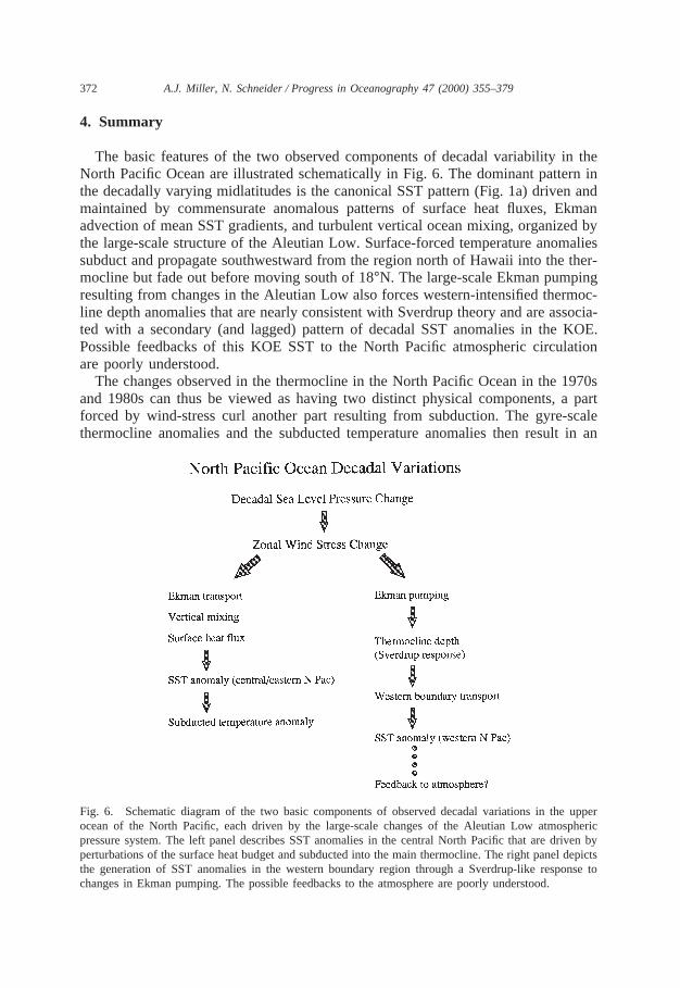
The basic features of the two observed components of decadal variability in theNorth Pacific Ocean are illustrated schematically in Fig. 6. The dominant pattern inthe decadally varying midlatitudes is the canonical SST pattern (Fig. 1a) driven andmaintained by commensurate anomalous patterns of surface heat fluxes, Ekmanadvection of mean SST gradients, and turbulent vertical ocean mixing, organized bythe large-scale structure of the Aleutian Low. Surface-forced temperature anomaliessubduct and propagate southwestward from the region north of Hawaii into the ther-mocline but fade out before moving south of 18°N. The large-scale Ekman pumpingresulting from changes in the Aleutian Low also forces western-intensified thermoc-line depth anomalies that are nearly consistent with Sverdrup theory and are associa-ted with a secondary (and lagged) pattern of decadal SST anomalies in the KOE.Possible feedbacks of this KOE SST to the North Pacific atmospheric circulationare poorly understood.

The changes observed in the thermocline in the North Pacific Ocean in the 1970sand 1980s can thus be viewed as having two distinct physical components, a partforced by wind-stress curl another part resulting from subduction. The gyre-scalethermocline anomalies and the subducted temperature anomalies then result in an

Fig. 6. Schematic diagram of the two basic components of observed decadal variations in the upperocean of the North Pacific, each driven by the large-scale changes of the Aleutian Low atmosphericpressure system. The left panel describes SST anomalies in the central North Pacific that are driven byperturbations of the surface heat budget and subducted into the main thermocline. The right panel depictsthe generation of SST anomalies in the western boundary region through a Sverdrup-like response tochanges in Ekman pumping. The possible feedbacks to the atmosphere are poorly understood.


apparent propagation of temperature from the KOE eastwards to 150°W andsouthwestwards towards the western boundary (Tourre et al., 1999). Since differentphysics controls the subsurface temperature anomalies in different regions, a gyre-scale circuit of temperature anomalies advected by the mean flow does not providean accurate description of the variability (cf. Zhang & Levitus, 1997). Moreover,the connection between the tropics and the midlatitude by anomalous subductioncannot be identified in the available dataset (Gu & Philander, 1997; Zhang,Rothstein & Busalacchi, 1998a).

Since anomalies of the central North Pacific canonical pattern lead KOE SSTanomalies by roughly five years, the decadal feedback mechanism suggested by Latifand Barnett (1994) must be re-evaluated. Determining the details of the response ofthe gyres (subpolar or subtropical) to the wind-stress curl forcing, the response ofthe SST to the gyre changes and the response of the atmosphere to the KOE SSTanomalies are now the key tasks for closing an intrinsic midlatitude decadal feedbackloop. A mixture of stochastic forcing by the atmosphere, direct forcing from tropicalatmospheric teleconnections and a weakly coupled gyre-circulation mode appear tobe the most consistent theoretical explanation for the observed decadal variabilityof the midlatitude Pacific Ocean during the 1970s–1990s. Determining the influenceof these complicated patterns on ecosystem dynamics is a major scientific goal forfuture decades.

Acknowledgements

Funding was provided by NSF (OCE97–11265), DOE (DE–FG03–98ER62605)and NOAA (NA47GP0188 and NA77RJ0453). We thank our many colleagues fordiscussions and for sharing results prior to publication. We greatly appreciate themany valuable comments provided in the reviews by Mike McPhaden and thesecond referee.

References

Adkison, M. D., Peterman, R. M., Lapointe, M. F., Gillis, D. M., & Korman, J. (1996). Alternative modelsof climatic effects on sockeye salmon,Oncorhynchus nerka, productivity in Bristol Bay, Alaska, andthe Fraser river, British Columbia.Fisheries Oceanography, 5, 137–152.

Alexander, M. A. (1992). Midlatitude atmosphere ocean interaction during El Nin˜o. 1. The North PacificOcean.Journal of Climate, 5, 944–958.

Auad, G., Miller, A. J., & White, W. B. (1998). Simulation of heat storages and associated heat budgets inthe Pacific Ocean — 2. Interdecadal timescale.Journal of Geophysical Research, 103, 27621–27636.

Barnett, T. P., Pierce, D. W., Saravanan, R., Schneider, N., Dommenget, D., & Latif, M. (1999). Originsof the midlatitude Pacific decadal variability.Geophysical Research Letters, 26, 1453–1456.

Barsugli, J. J., & Battisti, D. S. (1998). The basic effects of atmosphere–ocean thermal coupling onmidlatitude variability.Journal of the Atmospheric Sciences, 55, 477–493.

Baumgartner, T. R., Soutar, A., & Ferreira-Bartrina, V. (1992). Reconstruction of the history of Pacificsardine and Northern anchovy populations over the past 2 millennia from sediments of the


Santa-Barbara Basin, California.California Cooperative Oceanic Fisheries Investigations Reports, 33,24–40.

Beamish, R. J. (1995). Climate change and northern fish populations, Canadian Special Publication,Fish-eries and Aquatic Sciences, 121, 739 pp.

Beamish, R. J., & Bouillon, D. R. (1993). Pacific salmon production trends in relation to climate.CanadianJournal of Fisheries and Aquatic Sciences, 50, 1002–1016.

Beamish, R. J., Riddell, B. E., Neville, C. E. M., Thomson, B. L., & Zhang, Z. Y. (1995). Declines inChinook salmon catches in the Straight of Georgia in relation to shifts in the marine environment.Fisheries Oceanography, 4, 243–256.

Beamish, R. J., & McFarlane, G. A. (1989). Effects of ocean variability on recruitment and an evaluationof parameters used in stock assessment models. Canadian Special Publications,Fisheries and AquaticScience, 108, 379 pp.

Bitz, C. M., Battisti, D. S., Moritz, R. E., & Beesley, J. A. (1996). Low-frequency variability in the arcticatmosphere, sea ice, and upper-ocean climate system.Journal of Climate, 9, 394–408.

Bjerknes, J. (1966). A possible response to the atmospheric Hadley circulation to equatorial anomaliesof temperature.Tellus, 18, 820–829.

Bograd, S. J., Chereskin, T. K., & Roemmich, D. (2000). Transport of mass, heat, salt and nutrients inthe California Current System: annual cycle and interannual variability.Journal of GeophysicalResearch(in press).

Brodeur, R. D., & Ware, D. M. (1992). Interannual and interdecadal changes in zooplankton biomass inthe subarctic Pacific Ocean.Fisheries Oceanography, 1, 32–38.

Brodeur, R. D., Frost, B. W., Hare, S. R., Francis, R. C., & Ingraham, W. J. (1996). Interannual variationsin zooplankton biomass in the Gulf of Alaska, and covariation with California current zooplanktonbiomass.California Cooperative Oceanic Fisheries Investigations Reports, 37, 80–99.

Brodeur, R. D., Mills, C. E., Overland, J. E., Walters, G. E., & Schumacher, J. D. (1999). Evidence fora substantial increase in gelatinous zooplankton in the Bering Sea, with possible links to climatechange.Fisheries Oceanography, 8, 296–306.

Cayan, D. R., Miller, A. J., Barnett, T. P., Graham, N. E., Ritchie, J. N., & Oberhuber, J. M. (1995).Seasonal–interannual fluctuations in surface temperature over the Pacific: effects of monthly windsand heat fluxes. Natural Climate Variability on Decadal-to-Century Time Scales, National AcademyPress, Washington, DC, 133–150.

Cessi, P. (2000). Coupled dynamics of ocean currents and midlatitude storm tracks.Journal of Climate,13, 232–244.

Clarke, A. J., & Lebedev, A. (1999). Remotely driven decadal and longer changes in the coastal Pacificwaters of the Americas.Journal of Physical Oceanography, 29, 828–835.

Da Silva, A., Young, A. C., & Levitus, S. (1994). Atlas of Surface Marine Data, Volume 2: Anomaliesof Directly Observed Quantities. NOAA Atlas NESDIS 7, U.S. Department of Commerce, U.S. Gov.Printing Office, Washington, D.C. 416 pp.

Deser, C., & Blackmon, M. (1995). On the relationship between tropical and North Pacific sea surfacetemperature variations.Journal of Climate, 8, 1677–1680.

Deser, C., Alexander, M. A., & Timlin, M. S. (1996). Upper ocean thermal variations in the North Pacificduring 1970–1991.Journal of Climate, 9, 1840–1855.

Deser, C., Alexander, M. A., & Timlin, M. S. (1999). Evidence for a wind-driven intensification of theKuroshio Current Extension from the 1970s to the 1980s.Journal of Climate, 12, 1697–1706.

De Verdiere, A. C., & Huck, T. (1999). Baroclinic instability: an oceanic wavemaker for interdecadalvariability. Journal of Physical Oceanography, 27, 893–910.

Ebbesmeyer, C. C., Cayan, D. R., McLain, D. R., Nichols, F. H., Peterson, D. H., & Redmond, K. T.(1991). 1976 step in the Pacific climate: forty environmental changes between 1968–75 and 1977–1984. In:Proc. 7th Ann. Pacific Climate Workshop, California Department of Water Resources, Inter-agency Ecol. Stud. Prog. Report 26.

Enfield, D. B., & Mestas-Nun˜ez, A. M. (1999). Multiscale variabilities in global sea surface temperaturesand their relationships with tropospheric climate patterns.Journal of Climate, 12, 2719–2733.

Fine, R. A., Peterson, W. H., & Ostlund, H. G. (1987). The penetration of tritium into the tropical Pacific.Journal of Physical Oceanography, 17, 553–564.


Francis, R. C., & Hare, S. R. (1994). Decadal scale regime shifts in the large marine ecosystems of theNortheast Pacific: a case for historical science.Fisheries Oceanography, 3, 279–291.

Francis, R. C., Hare, S. R., Hollowed, A. B., & Wooster, W. S. (1998). Effects of interdecadal climatevariability on the oceanic ecosystems of the NE Pacific.Fisheries Oceanography, 7, 1–21.

Frankignoul, C., & Hasselmann, K. (1977). Stochastic climate models. Part II. Application to SST anomal-ies and thermocline variability.Tellus, 29, 289–305.

Frankignoul, C., Mu¨ller, P., & Zorita, E. (1997). A simple model of the decadal response of the oceanto stochastic wind forcing.Journal of Physical Oceanography, 27, 1533–1546.

Freeland, H., Denman, K., Wong, C. S., Whitney, F., & Jacques, R. (1997). Evidence of change in thewinter mixed layer in the Northeast Pacific Ocean.Deep-Sea Research I, 44, 2117–2129.

Gargett, A. E. (1997). The optimal stability window: a mechanism underlying decadal fluctuations inNorth Pacific salmon stocks?Fisheries Oceanography, 6, 109–117.

Gargett, A. E., Li, M., & Brown, R. (1998). Testing the concept of an optimal stability window. BioticImpacts of Extratropical Climate Change in the Pacific. Aha Huliko’a Hawaiian Winter Workshop,University of Hawaii, SOEST Special Publication, 133–140.

Giese, B. S., & Carton, J. A. (1999). Interannual and decadal variability in the tropical and midlatitudePacific Ocean.Journal of Climate, 12, 3402–3418.

Goodman, J., & Marshall, J. (1998). A model of decadal middle-latitude atmosphere–ocean coupledmodes.Journal of Climate, 12, 621–641.

Graham, N. E. (1994). Decadal scale variability in the 1970s and 1980s: observations and model results.Climate Dynamics, 10, 135–162.

Graham, N. E., Barnett, T. P., Wilde, R., Ponater, M., & Schubert, S. (1994). Low-frequency variabilityin the winter circulation over the Northern Hemisphere.Journal of Climate, 7, 1416–1442.

Gu, D. F., & Philander, S. G. H. (1997). Interdecadal climate fluctuations that depend on exchangesbetween the tropics and extratropics.Science, 275, 805–807.

Hare, S. R., & Francis, R. C. (1995). Climate change and salmon production in the Northeast PacificOcean. In R. J. Beamish (Ed.),Climate change and northern fish populations(pp. 357–372). CanadianSpecial Publication of Fisheries and Aquatic Sciences, 121.

Hare, S. R., & Mantua, N. J. (2000). Empirical evidence for North Pacific regime shifts in 1977 and1989.Progress in Oceanography, 47, 103–145.

Hare, S. R., Mantua, N. J., & Francis, R. C. (1999). Inverse production regimes: Alaska and West CoastPacific salmon.Fisheries, 24, 6–14.

Hanawa, K. (1995). Southward penetration of the Oyashio water system and the wintertime condition ofmidlatitude westerlies over the North Pacific.Bulletin of the Hokkaido National Fisheries Institute,59, 103–120.

Hasselmann, K. (1976). Stochastic climate models. Part I. Theory.Tellus, 28, 473–485.Hayward, T. L. (1997). Pacific Ocean climate change: atmospheric forcing, ocean circulation and ecosys-

tem response.Trends in Ecology and Evolution, 12, 150–154.Hazeleger, W. (1999).Variability in mode water formation on the decadal time scale. Ph.D. Dissertation,

University of Utrecht. 144 pp.Holbrook, S. J., Schmitt, R. J., & Stephens, J. S. (1997). Changes in an assemblage of temperate reef

fishes associated with a climate shift.Ecological Applications, 7, 1299–1310.Holland, W. R., & Haidvogel, D. B. (1981). On the vacillation of an unstable baroclinic wave field in

an eddy-resolving model of the oceanic general circulation.Journal of Physical Oceanography, 11,557–568.

Holloway, G., & Muller, P. (1998). Biotic impacts of extratropical climate change in the Pacific. AhaHuliko’a Hawaiian Winter Workshop, University of Hawaii, SOEST Special Publication, 156 pp.

Hollowed, A. B., & Wooster, W. S. (1992). Variability of winter ocean conditions and strong year classesof Northeast Pacific groundfish.ICES Marine Science Symposium, 195, 433–444.

Hollowed, A. B., & Wooster, W. S. (1995). Decadal-scale variations in the eastern subarctic Pacific: II.Response of Northeast Pacific fish stocks. In R. J. Beamish (Ed.),Climate change and northern fishpopulations(pp. 373–385). Canadian Special Publication of Fisheries and Aquatic Sciences, 121.

Inui, T., & Takeuchi, K. (1999). A numerical investigation of the subduction process in response to anabrupt intensification of the westerlies.Journal of Physical Oceanography, 29, 1993–2015.


Jacobs, G. A., Hurlburt, H. E., Kindle, J. C., Metzger, E. J., Mitchell, J. L., Teague, W. J., & Wallcraft,A. J. (1994). Decade-scale trans-Pacific propagation and warming effects of an El Nin˜o anomaly.Nature, London, 370, 360–363.

James, I. N., & James, P. M. (1989). Ultra-low-frequency variability in a simple atmospheric model.Nature, London, 342, 53–55.

Jiang, S., Jin, F.-F., & Ghil, M. (1995). Multiple equilibria, periodic and aperiodic solutions in a wind-driven, double-gyre, shallow-water model.Journal of Physical Oceanography, 25, 764–786.

Jin, F.-F. (1997). A theory of interdecadal climate variability of the North Pacific ocean–atmospheresystem.Journal of Climate, 10, 1821–1835.

Johnson, G. C., & McPhaden, M. J. (1999). Interior pycnocline flow from the subtropical to the equatorialPacific Ocean.Journal of Physical Oceanography, 29, 3073–3089.

Karl, D. M. (1999). A sea of change: biogeochemical variability in the North Pacific subtropical gyre.Ecosystems, 2, 181–214.

Kessler, W. S. (1999). Interannual variability of the subsurface high salinity tongue south of the equatorat 165°E. Journal of Physical Oceanography, 29, 2038–2049.

Kleeman, R., McCreary, J. P., & Klinger, B. A. (1999). A mechanism for generating ENSO decadalvariability. Geophysical Research Letters, 26, 1743–1746.

Knutson, T. R., & Manabe, S. (1998). Model assessment of decadal variability and trends in the tropicalPacific Ocean.Journal of Climate, 11, 2273–2296.

Lagerloef, G. S. E. (1995). Interdecadal variations in the Alaska Gyre.Journal of Physical Oceanography,25, 2242–2258.

Latif, M. (1998). Dynamics of interdecadal variability in coupled ocean–atmosphere models.Journal ofClimate, 11, 602–624.

Latif, M., & Barnett, T. P. (1994). Causes of decadal climate variability over the North Pacific and NorthAmerica.Science, 266, 634–637.

Latif, M., & Barnett, T. P. (1996). Decadal climate variability over the North Pacific and North America:dynamics and predictability.Journal of Climate, 9, 2407–2423.

Lau, N. C. (1997). Interactions between global SST anomalies and the midlatitude atmospheric circulation.Bulletin of the American Meteorological Society, 78, 21–33.

Lavaniegos, B. E., Gomez-Gutierrez, J., Lara-Lara, J. R., & Hernandez-Vazquez, S. (1998). Long-termchanges in zooplankton volumes in the California Current System — the Baja California region.Marine Ecology, 169, 55–64.

Liu, Z. (1999). Forced planetary wave response in a thermocline gyre.Journal of Physical Oceanography,29, 1036–1055.

Liu, Z., & Shin, S.-I. (1999). On thermocline ventilation of active and passive tracers.GeophysicalResearch Letters, 26, 357–360.

Liu, Z., Philander, S. G. H., & Pacanowski, R. (1994). A GCM study of tropical–subtropical upper oceanmass exchange.Journal of Physical Oceanography, 24, 2606–2623.

Lluch-Belda, D., Lluch-Cota, D. B., Hernandez-Vazquez, S., & Salinas-Zavala, C. A. (1992). Sardinepopulation expansion in eastern boundary systems of the Pacific Ocean as related to sea surface tem-perature.South African Journal of Marine Sciences, 12, 147–155.

Lu, P., McCreary, J. P., & Klinger, B. A. (1998). Meridional circulation cells and the source waters ofthe Pacific Equatorial Undercurrent.Journal of Physical Oceanography, 28, 62–84.

Lysne, J., Chang, P., & Giese, B. (1997). Impact of the extratropical Pacific on equatorial variability.Geophysical Research Letters, 24, 2589–2592.

Mann, M. E., & Park, J. (1996). Joint spatiotemporal modes of surface temperature and sea level pressurevariability in the Northern Hemisphere during the last century.Journal of Climate, 9, 2137–2162.

Mantua, N. J., Hare, S. R., Zhang, Y., Wallace, J. M., & Francis, R. C. (1997). A Pacific interdecadalclimate oscillation with impacts on salmon production.Bulletin of the American MeteorologicalSociety, 78, 1069–1079.

McCreary, J. P., & Lu, P. (1994). Interaction between the subtropical and equatorial oecan circulation —the subtropical cell.Journal of Physical Oceanography, 24, 466–497.

McGowan, J. A., Cayan, D. R., & Dorman, L. M. (1998). Climate–ocean variability and ecosystemresponse in the northeast Pacific.Sciences, 281, 210–217.


Meacham, S. P., Dewar, W. K., & Chassignet, E. (1998). Low-frequency variability in the midlatitudecoupled atmosphere–ocean system (abstract), EOS, Transactions of the American Geophysical Union,79 Ocean Sci. Meet. Suppl., OS36.

Meyers, S. D., Johnson, M. A., Liu, M., O’Brien, J. J., & Spiesberger, J. L. (1996). Interdecadal variabilityin a numerical model of the northeast Pacific Ocean: 1970–89.Journal of Physical Oceanography,26, 2635–2652.

Miller, A. J. (1992). Large-scale ocean–atmosphere interactions in a simplified coupled model of themidlatitude wintertime circulation.Journal of the Atmospheric Sciences, 49, 273–286.

Miller, A. J., Cayan, D. R., Barnett, T. P., Graham, N. E., & Oberhuber, J. M. (1994a). Interdecadalvariability of the Pacific Ocean: model response to observed heat flux and wind stress anomalies.Climate Dynamics, 9, 287–302.

Miller, A. J., Cayan, D. R., Barnett, T. P., Graham, N. E., & Oberhuber, J. M. (1994b). The 1976–77climate shift of the Pacific Ocean.Oceanography, 7, 21–26.

Miller, A. J., White, W. B., & Cayan, D. R. (1997). North Pacific thermocline variations on ENSO timescales.Journal of Physical Oceanography, 27, 2023–2039.

Miller, A. J., Cayan, D. R., & White, W. B. (1998). A westward intensified decadal in the North Pacificthermocline and gyre-scale circulation.Journal of Climate, 11, 3112–3127.

Minobe, S. (1999). Resonance in bidecadal and pentadecadal climate oscillations over the North Pacific:role in climatic regime shifts.Geophysical Research Letters, 26, 855–858.

Mullin, M. M. (1998). Interannual and interdecadal variation in California Current zooplankton:Calanusin the late 1950s and early 1990s.Global Change Biology, 4, 115–119.

Munk, W. (1981). Internal waves and small-scale processes. In B. A. Warren, & C. Wunsch,Evolutionof physical oceanography(pp. 264–291). Cambridge, MA: MIT Press.

Munnich, M., Latif, M., Venzke, S., & Maier-Reimer, E. (1998). Decadal oscillations in a simple coupledmodel.Journal of Climate, 11, 3309–3319.

Mysak, L. A., & Venegas, S. A. (1998). Decadal climate oscillations in the Arctic: a new feedback loopfor atmosphere–ice–ocean interactions.Geophysical Research Letters, 25, 3607–3610.

Nakamura, H., Lin, G., & Yamagata, T. (1997). Decadal climate variability in the North Pacific duringrecent decades.Bulletin of the American Meteorological Society, 78, 2215–2225.

Neelin, J. D., & Weng, W. J. (1999). Analytical prototypes for ocean–atmosphere interaction at midlati-tudes. Part I: coupled feedbacks as a sea surface temperature dependent stochastic process.Journalof Climate, 12, 697–721.

Overland, J. E., Salo, S., & Adams, J. R. (1999). Salinity signature of the Pacific Decadal Oscillation.Geophysical Research Letters, 26, 1337–1340.

Palmer, T., & Sun, Z. (1985). A modeling and observational study of the relationship between SSTin the north-west Atlantic and the atmospheric general circulation.Quarterly Journal of the RoyalMeteorological Society, 111, 947–975.

Peng, S., Robinson, W. A., & Hoerling, M. P. (1997). The modeled atmospheric response to midlatitudeSST anomalies and its dependence on background circulation states.Journal of Climate, 10, 971–987.

Pierce, D. W., Barnett, T. P., & Latif, M. (2000). Connections between the Pacific Ocean tropics andmidlatitudes on decadal time scales.Journal of Climate, 13, 1173–1194.

Polovina, J., Mitchum, G. T., Graham, N. E., Craig, M. P., DeMartini, E. E., & Flint, E. N. (1994).Physical and biological consequences of a climatic event in the Central North Pacific.Fisheries Ocean-ography, 3, 15–21.

Polovina, J., Mitchum, G. T., & Evans, G. T. (1995). Decadal and basin-scale variations in mixed layerdepth and the impact on biological production in the Central and North Pacific.Deep-Sea ResearchI, 42, 1701–1716.

Qiu, B., & Joyce, T. M. (1992). Interannual variability in the mid- and low-latitude Western North Pacific.Journal of Physical Oceanography, 22, 1062–1079.

Robertson, A. W. (1996). Interdecadal variability over the North Pacific in a multi-century climate simu-lation. Climate Dynamics, 12, 227–241.

Roemmich, D., & McGowan, J. (1995). Climatic warming and the decline of zooplankton in the CaliforniaCurrent.Science, 267, 1324–1326.

Rothstein, L. M., Zhang, R. H., Busalacchi, A. J., & Chen, D. (1998). A numerical simulation of the


mean water pathways in the subtropical and tropical Pacific Ocean.Journal of Physical Oceanography,28, 322–343.

Royer, T. C. (1981). Baroclinic transport in the Gulf of Alaska Part II. A fresh water driven coastalcurrent.Journal of Marine Research, 39, 251–266.

Sagarin, R. D., Barry, J. P., Gilman, S. E., & Baxter, C. H. (1999). Climate-related change in an intertidalcommunity over short and long time scales.Ecological Monographs, 69, 465–490.

Saravanan, R., & McWilliams, J. C. (1998). Advective ocean–atmosphere interaction: an analytical stoch-astic model with implications for decadal variability.Journal of Climate, 11, 165–188.

Schneider, N. (2000). A decadal spiciness mode in the tropics.Geophysical Research Letters, 27, 257–260.Schneider, N. S., Miller, A. J., Alexander, M. A., & Deser, C. (1999a). Subduction of decadal North

Pacific temperature anomalies: observations and dynamics.Journal of Physical Oceanography, 29,1056–1070.

Schneider, N. S., Venzke, S., Miller, A. J., Pierce, D. W., Barnett, T. P., Deser, C., & Latif, M. (1999b).Pacific thermocline bridge revisited.Geophysical Research Letters, 26, 1329–1332.

Schwing, F. B. (1998). Patterns and mechanisms for climate change in the North Pacific: the wind didit. Biotic Impacts of Extratropical Climate Change in the Pacific. Aha Huliko’a Hawaiian WinterWorkshop, University of Hawaii, SOEST Special Publication, 29–36.

Schwing, F. B., & Mendelsohn, R. (1997). Increased coastal upwelling in the California Current system.Journal of Geophysical Research, 102, 12785–12786.

Sekine, Y. (1988). Anomalous southward intrusion of the Oyashio east of Japan. I. Influence of theinterannual and seasonal variations in the wind stress over the North Pacific.Journal of GeophysicalResearch, 93, 2247–2255.

Shin, S.-I., & Liu, Z. (2000). On the response of the equatorial thermocline to extratropical buoyancyforcing. Journal of Physical Oceanography(in press).

Smith, K. L., & Kaufmann, R. S. (1999). Long-term discrepancy between food supply and demand inthe deep eastern North Pacific.Science, 284, 1174–1177.

Spall, M. A. (1996). Dynamics of the Gulf Stream/Deep western boundary current crossover. Part II:low-frequency internal oscillations.Journal of Physical Oceanography, 26, 2169–2182.

Suga, T., Kato, A., & Hanawa, K. (2000). North Pacific Tropical Water: its climatology and temporalchanges associated with the climate regime shift in the 1970s.Progress in Oceanography, 47, 227–256.

Sugimoto, T., & Tadokoro, K. (1997). Interannual–interdecadal variations in zooplankton biomass, chloro-phyll concentration and physical environment in the subarctic Pacific and Bering Sea.Fisheries Ocean-ography, 6, 74–93.

Sydeman, W. J., & Allen, S. G. (1999). Pinniped population dynamics in central California: correlationswith sea surface temperature and upwelling indices.Science, 284, 1174–1177.

Tabata, S. (1991). Annual and interannual variability of baroclinic transports across Line P in the northeastPacific Ocean.Deep-Sea Research, 38 (Suppl. 1), S221–S245.

Talley, L. (1999). Simple coupled mid-latitude climate models.Journal of Physical Oceanography, 29,2016–2037.

Tanimoto, Y., Iwasaka, N., Hanawa, K., & Toba, Y. (1992). Characteristic variations of sea surfacetemperature with multiple time scales in the North Pacific.Journal of Climate, 6, 1153–1160.

Thompson, D. W. J., & Wallace, J. M. (1998). The Arctic Oscillation signature in the wintertime geo-potential height and temperature fields.Geophysical Research Letters, 25, 1297–1300.

Tourre, Y., White, W. B., & Kushnir, Y. (1999). Evolution of interdecadal variability in sea level pressure,sea surface temperature, and upper ocean temperature over the Pacific Ocean.Journal of PhysicalOceanography, 29, 1528–1541.

Trenberth, K. E. (1990). Recent observed interdecadal climate changes in the Northern Hemisphere.Bull-etin of the American Meteorological Society, 71, 988–993.

Trenberth, K. E. (1991). Recent climate changes in the Northern Hemisphere. In M. E. Schlesinger,Greenhouse-gas-induced climatic change: a critical appraisal of simulations and observations(pp.377–390). Amsterdam: Elsevier.

Trenberth, K. E., & Hurrell, J. W. (1994). Decadal atmosphere–ocean variations in the Pacific.ClimateDynamics, 9, 303–319.


Tsonis, A. A., Roebber, P. J., & Elsner, J. B. (1999). Long-range correlations in the extratropical atmos-pheric circulation: Origins and implications.Journal of Climate, 12, 1534–1541.

Tziperman, E., Cane, M. A., & Zebiak, S. E. (1995). Irregularity and locking to the seasonal cycle in anENSO prediction model as explained by the quasi-periodicity route to chaos.Journal of the Atmos-pheric Sciences, 52, 293–306.

Venrick, E. L., McGowan, J. A., Cayan, D. R., & Hayward, T. L. (1987). Climate and chlorophyll a:long-term trends in the central north Pacific Ocean.Science, 238, 70–72.

Veit, R. R., Mcgowan, J. A., Ainley, D. G., Wahls, T. R., & Pyle, P. (1997). Apex marine predatordeclines ninety percent in association with changing oceanic climate.Global Change Biology, 3,23–28.

Venzke, S. (1999).Ocean–atmosphere interactions on decadal timescales. Ph.D. Dissertation, Universita¨tHamburg. 99 pp.

Wang, C. Z., & Weisberg, R. H. (1998). Climate variability of the coupled tropical–extratropical ocean–atmosphere system.Geophysical Research Letters, 25, 3979–3982.

Watanabe, M., & Kimoto, M. (2000). Behavior of midlatitude decadal oscillations in a simple atmosphere–ocean system.Journal of the Meteorological Society of Japan, (in press).

Watanabe, T., & Mizuno, K. (1994). Decadal changes of the thermal structure in the North Pacific.International WOCE Newsletter, 15, 10–13.

Weinheimer, A. L., Kennett, J. P., & Cayan, D. R. (1999). Recent increase in surface-water stabilityduring warming off California as recorded in marine sediments.Geology, 27, 1019–1022.

White, W. B. (1995). Design of a global observing system for gyre-scale upper ocean temperature varia-bility. Progress in Oceanography, 36, 169–217.

White, W. B., & Cayan, D. R. (1998). Quasi-periodicity and global symmetries in interdecadal upperocean temperature variability.Journal of Geophysical Research, 103, 21335–21354.

White, W. B., Lean, J., Cayan, D. R., & Dettinger, M. D. (1997). Response of global upper ocean tempera-ture to changing solar irradiance.Journal of Geophysical Research, 102, 3255–3266.

Wu, J. Q., & Hsieh, W. W. (1999). A modelling study of the 1976 climate regime shift in the NorthPacific Ocean.Canadian Journal of Fisheries and Aquatic Sciences, 56, 2450–2462.

Wunsch, C. (1999). The interpretation of short climate records, with comments on the North Atlantic andSouthern Oscillations.Bulletin of the American Meteorological Society, 80, 245–255.

Wyllie-Echeverria, T., & Wooster, W. S. (1998). Year to-year variations in Bering Sea ice cover andsome consequences for fish distributions.Fisheries Oceanography, 7, 159–170.

Xie, S.-P., Kunitani, T., Kubokawa, A., Nonaka, M., & Hosoda, S. (2000). Interdecadal thermoclinevariability in the North Pacific for 1958–1997: a GCM simulation.Journal of Physical Oceanography(in press).

Xu, W., Barnett, T. P., & Latif, M. (1998). Decadal variability in the North Pacific as simulated by ahybrid coupled model.Journal of Climate, 11, 297–312.

Yasuda, T., & Hanawa, K. (1997). Decadal changes in the mode waters in the midlatitude North Pacific.Journal of Physical Oceanography, 27, 858–870.

Yukimoto, S., Endoh, M., Kitamura, Y., Kitoh, A., Motoi, T., Noda, A., & Tokioka, T. (1996). Interannualand interdecadal variabilities in the Pacific in an MRI coupled GCM.Climate Dynamics, 12, 667–683.

Zhang, R. H., & Levitus, S. (1997). Structure and cycle of decadal variability of upper-ocean temperaturein the North Pacific.Journal of Climate, 10, 710–727.

Zhang, Y., Wallace, J. M., & Battisti, D. S. (1997). ENSO-like interdecadal variability: 1900-93.Journalof Climate, 10, 1004–1020.

Zhang, R. H., Rothstein, L. M., & Busalacchi, A. J. (1998a). Origin of upper-ocean warming and El Nin˜ochange on decadal scales in the tropical Pacific Ocean.Nature, London, 391, 879–883.

Zhang, X. B., Sheng, J., & Shabbar, A. (1998b). Modes of interannual and interdecadal variability ofPacific SST.Journal of Climate, 11, 2556–2569.

Zhang, R. H., & Liu, Z. (1999). Decadal thermocline variability in the North Pacific Ocean: two pathwaysaround the subtropical gyre.Journal of Climate, 12, 3273–3296.

interdecadal climate regime dynamics in the north pacific ocean: theories, observations and...

Documents