Interchange Rearrangement: The Element-CostModel

Oren Kapah2, Gad M. Landau1,5,?, Avivit Levy3,4,??, and Nitsan Oz1

1 Department of Computer Science, University of Haifa, Haifa 31905, Israel. Phone:(972-4) 824-0103, FAX: (972-4) 824-9331; E-mail: landau@cs.haifa.ac.il,

nitsan@cri.haifa.ac.il2 Department of Computer Science, Bar Ilan University, Ramat Gan 52900, Israel.

E-mail: kapaho@cs.biu.ac.il3 Department of Software Engineering, Shenkar College, 12 Anna Frank,

Ramat-Gan, 52526, Israel. E-mail: avivitlevy@shenkar.ac.il4 CRI, University of Haifa, Haifa 31905, Israel.

5 Department of Computer and Information Science, Polytechnic Institute of NYU,Six MetroTech Center, Brooklyn, NY 11201-3840

Abstract. Given an input string S and a target string T when S is apermutation of T , the interchange rearrangement problem is to apply onS a sequence of interchanges, such that S is transformed into T . Theinterchange operation exchanges the position of the two elements onwhich it is applied. The goal is to transform S into T at the minimum costpossible, referred to as the distance between S and T . The distance can bedefined by several cost models that determine the cost of every operation.There are two known models: The Unit-cost model and the Length-costmodel. In this paper, we suggest a natural cost model: The Element-cost model. In this model, the cost of an operation is determined by theelements that participate in it. Though this model has been studied inother fields, it has never been considered in the context of rearrangementproblems. We consider both the special case where all elements in Sand T are distinct, referred to as a permutation string, and the generalcase, referred to as a general string. An efficient optimal algorithm forthe permutation string case and efficient approximation algorithms forthe general string case, which is NP-hard, are presented. The studyis broadened to include the transposition rearrangement problem underthe Element-cost model and under the other known models, in order toprovide additional perspective on the new model.

Keywords: strings rearrangement distances, rearrangement cost mod-els, interchange rearrangement.

? partially supported by the Israel Science Foundation grant 35/05 and the Israel-Korea Scientific Research Cooperation.

?? Corresponding author

1 Introduction

The problem of defining the distance or similarity between two strings Sand T has been studied extensively over the years. There are many knownand established methods, such as the Edit distance and the Hammingdistance [13]. The Edit distance allows three operations (substitution,insertion or deletion) upon the input string. There are several general-izations of the basic Edit distance (also referred to as the Levenshteindistance), which defines a unit-cost for every operation. One is the theoperation-weight edit distance, which gives a unit-cost for every type ofoperation. Another is the alphabet-weight edit distance, which defines acost for every operation depending on the elements participating in thespecific operation.

These string metrics deal with errors of data appearing in the text andgive a measure of either similarity or distance between an input string Sand a target string T . The order of the elements is assumed to be correct.However, address errors may also be considered ([1–4]). In these types oferrors, elements in S may only be mispositioned. It is commonly assumedthat the input string is a permutation of the target string in order tohave a finite distance. In the rearrangement problem, it is assumed thatonly address errors have occurred. The goal is to apply a sequence of legaloperations on S, such that S is transformed into T at the minimum costpossible, referred to as the distance between S and T .

The interchange rearrangement problem was studied by Cayley [9].Cayley solved this problem for permutation strings under the Unit-costmodel and left the problem of general strings as an open problem. Re-cently, Amir et al. solved Cayley’s open problem by showing it isNP-hardand giving a 1.5-approximation algorithm. In addition, they extended thisproblem by examining it under the Length-cost model [4]. In this paper,we further extend this problem on both permutation strings and generalstrings by examining it under the Element-cost model.

Formal Definitions. We begin with formal definitions of the interchangeoperator and the Element-cost model.

Definition 1. Let S = s1, . . . , sn be a string. An interchangeof elements si and sj, i < j, transforms S into S′ =s1, . . . , si−1, sj , si+1, . . . , sj−1, si, sj+1, . . . , sn.

Cost Models. There are two known cost models in the context of re-arrangement problems. In the Unit-cost model (UCM) each operation is

given a unit cost, so the problem is to transform S into T with a minimumnumber of operations. In the Length-cost model (LCM), the cost of an op-eration depends on its length characteristic. Other characteristics may beconsidered in the rearrangement problem. For example, some elementsmay be heavier than other elements. In such cases, moving light elementsis preferable to moving heavy elements. This observation motivated re-searchers to explore the Element-cost model (ECM). In [12], Gupta andKumar considered the problem of sorting and selection in the compari-son model for structured costs. In their work, they assumed that everyelement has a weight and that the cost of a comparison is defined by afunction applied to the weight of the elements that participate in the com-parison. They gave approximations for the optimal solution for families ofstructured functions such as summation, multiplication, etc. Recently, [5]addressed the same problem of sorting and selection for random costs.However, this paper is the first to consider the ECM for dealing withrearrangement problems.

Definition 2. Let w : Σ → R+ be a weight function, which assigns anon-negative weight to every element in Σ. Let g : Σ × Σ → R+ be afunction defining the interchange cost. The function g is called a generalfunction if it satisfies the following conditions:

1. ∀x, y ∈ Σ : g(x, y) = g(y, x).2. ∀x, y, z ∈ Σ : w(y) ≤ w(z)⇔ g(x, y) ≤ g(x, z).

The summation function g(x, y) = w(x) + w(y) and the multiplicationfunction g(x, y) = w(x) ·w(y) are two examples of intuitive general func-tions. The technique used in the interchange rearrangement problem un-der the ECM is different than the one used under the UCM. Considerthe example shown in Figure 1. In this example, an optimal rearrange-ment is given when the UCM is used - S is transformed into T using 3interchanges (Figure 1(a)). When the ECM is used, the same sequence ofinterchanges costs 900, whereas the alternative sequence of interchangessuggested performs 5 interchanges and costs only 850 (Figure 1(b)).

If all elements in S are distinct, a unique bijection f : S → {1, . . . , n}can be defined such that f(si) equals the position of the element si inT . Thus S can be represented by π = f(s1), f(s2), . . . , f(sn) and T by1, . . . , n. For this case the term permutation string is used. The inputstring is then assumed to be π, i.e, a permutation of 1, . . . , n. Under thisassumption the rearrangement problem is simply a sorting problem, i.e.the distance is the minimum cost for sorting π. Problems of sorting apermutation string have been studied extensively [6–8, 10, 14, 15]. For the

edcbaT

decbaS

debcaS

bedcaS

100 200 200 100 10

edcba

UCM

(a)

edcbaT

eacbdS

aecbdS

becadS

beacdS

bedcaS

ECM

(b)

Fig. 1. In both (a) and (b), every row represents a stage in the rearrangement. Theelements marked with circles are the elements interchanged to establish the next stage.In (a), the goal is to transform S into T with a minimum number of interchanges(UCM ). This is done by applying 3 interchanges. In (b), the ECM is used. Everyelement has a weight and the cost of an interchange is the sum of the weights. Thesequence of interchanges applied in (a) costs 900, whereas the sequence of 5 interchangesapplied in (b) costs 850.

general case in which S may have repetitions of elements, the term generalstring is used.

Results. Our main results are:

1. O(n) time algorithm for the interchange rearrangement problem forpermutation strings for any general function.

2. NP-hardness for the interchange rearrangement problem for generalstrings:(a) O(n) time 3-approximation algorithm for any general function.(b) O(n · lg |Σ|) time 1.72-approximation algorithm for the summation

function.

We also broaden the study to include the transposition rearrangementproblem under the ECM, UCM and the LCM for general strings andpermutation strings. Table 1 summarizes the known and new results.

The paper is organized as follows. Section 2 gives additional prelimi-naries and notations. Section 3 presents an algorithm for the interchangerearrangement problem for permutation strings for any general function.

Section 4 presents an approximation algorithm for the interchange rear-rangement problem for general strings for any general function and animproved approximation algorithm for the summation function. Finally,Section 5 presents a simple extension of the transposition rearrangementproblem under the ECM, UCM and the LCM in order to give additionalperspective on the new model.

Table 1. A Summary of Results

UCM ECM LCM

Interchanges

Permutation O(n) [9] O(n) for a general function O(n) [4]Strings

General NP-hard [4] NP-hard O(n) [4]Strings O(n · lg |Σ|) 1.5-approx. [4] O(n) 3-approx.

for a general functionO(n · lg |Σ|) 1.72-approx.

for the summation function

Transpositions

Permutation O(n lgn) [14] O(n lgn) O(n lgn)Strings

General O(n2) O(n2) O(n lgn)Strings

2 Preliminaries and Notations

Given an input string S and a target string T , we define a multi-graphGS,T = (V,E) (see Fig. 2) in the following way: V = {v ∈ Σ : v appearsin S and T} and E = {(ti, si), 1 ≤ i ≤ n}. In other words, every dis-tinct character has a vertex and for every index 1 ≤ i ≤ n there is anedge connecting the vertex representing ti with the vertex of si, meaningthat by the end of the rearrangement process, si will be moved and re-placed by a ti character. Since S and T have the same quantities of eachelement of Σ, the number of incoming edges of every vertex equals thenumber of its outgoing edges, which is the number of occurrences of thevertex’s character in S (and hence in T ). Therefore, each of the stronglyconnected components of G(S, T ) is an Eulerian directed graph and bydefinition can be decomposed into edge-disjoint directed cycles. If S isa permutation string, every vertex has exactly one incoming edge andone outgoing edge and therefore, GS,T can be uniquely decomposed into

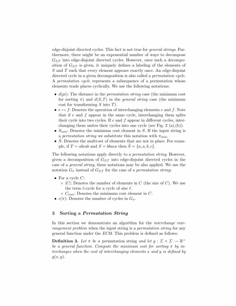
edge-disjoint directed cycles. This fact is not true for general strings. Fur-thermore, there might be an exponential number of ways to decomposeGS,T into edge-disjoint directed cycles. However, once such a decompo-sition of GS,T is given, it uniquely defines a labeling of the elements ofS and T such that every element appears exactly once. An edge-disjointdirected cycle in a given decomposition is also called a permutation cycle.A permutation cycle represents a subsequence of a permutation whoseelements trade places cyclically. We use the following notations:

• d(pi): The distance in the permutation string case (the minimum costfor sorting π) and d(S, T ) in the general string case (the minimumcost for transforming S into T ).• e↔ f : Denotes the operation of interchanging elements e and f . Note

that if e and f appear in the same cycle, interchanging them splitstheir cycle into two cycles. If e and f appear in different cycles, inter-changing them unites their cycles into one cycle (see Fig. 2 (a),(b)).• Smin: Denotes the minimum cost element in S. If the input string is

a permutation string we substitute this notation with πmin.• S̃: Denotes the multi-set of elements that are not in place. For exam-

ple, if T = abcab and S = bbaca then S̃ = {a, a, b, c}.

The following notations apply directly to a permutation string. However,given a decomposition of GS,T into edge-disjoint directed cycles in thecase of a general string, these notations may be also applied. We use thenotation Gπ instead of GS,T for the case of a permutation string :

• For a cycle C:◦ |C|: Denotes the number of elements in C (the size of C). We use

the term `-cycle for a cycle of size `.◦ Cmin: Denotes the minimum cost element in C.

• c(π): Denotes the number of cycles in Gπ.

3 Sorting a Permutation String

In this section we demonstrate an algorithm for the interchange rear-rangement problem when the input string is a permutation string for anygeneral function under the ECM. This problem is defined as follows:

Definition 3. Let π be a permutation string and let g : Σ × Σ → R+

be a general function. Compute the minimum cost for sorting π by in-terchanges when the cost of interchanging elements x and y is defined byg(x, y).

52674183

87654321

S

T

↓↓↓↓↓↓↓↓

4 67

2

8

5

1

3

14413232

33212441

S

T

↓↓↓↓↓↓↓↓

)(a

)(b

1

4

3 2

12

4

3

4

2

3

1

1

2

4 3

1

3

4

2

4 67

2

3

5

1

8

83↔

52674138

87654321

S

T

↓↓↓↓↓↓↓↓

)(c

Fig. 2. In (a) and (b), S is a permutation string. Thus, every vertex in Gπ has exactlyone incoming edge and one outgoing edge and Gπ is in fact the unique edge-disjointdirected cycles decomposition. Interchanging 3 ↔ 8 in (a) splits their cycle into twocycles as shown in (b). The same interchange in (b) unites their two cycles into onecycle, as shown in (a). In (c), S is a general string and is a permutation of T . Therefore,the number of incoming edges equals the number of outgoing edges and equals thenumber of occurrences in S (or in T ). Hence, GS,T is an Eulerian directed graph, andcan be decomposed into edge-disjoint directed cycles. However, this decomposition isnot unique.

Cayley [9] studied this problem under the UCM. He showed that givena permutation π, the minimum number of interchanges needed for sort-ing π, is n − c(π). This is achieved by interchanging only elements thatshare a cycle until there are no such elements (the permutation is sorted).When the ECM is used, one might also be inclined to apply a minimumnumber of interchanges. This inclination implies that one would be mak-ing interchanges only within cycles. Any interchange between elements ofdifferent cycles would result in an increase in the number of interchangesneeded for sorting π and probably in the total cost for sorting π. However,this inclination is incorrect. Moreover, there might be cases in which theoptimal solution would be to increase the number of interchanges needed

for sorting π in order to decrease the total cost. We will describe an algo-rithm for sorting a permutation string by interchanges under ECM, andthen prove that it yields the optimal cost, i.e., the distance d(π).

3.1 The O(n) time algorithm

The basic idea of the CEAps algorithm (Fig. 4) is quite simple. In order tosort the permutation π at a minimum cost, either the cheapest element insome cycle is used to sort all the other elements including itself, or (if thecheapest element in the cycle is not cheap enough) the cost for introducingthe cycle to the cheapest element in π is ”paid” by interchanging it withthe cheapest element of the cycle. Doing so unites the cycle with the cycleof the minimum cost element of π. Then the cheapest element of π canbe used to sort all the other elements in the cycle. We call this algorithm”The Cheapest Employee Algorithm” (CEA).

Definition 4. Let C be a cycle in Gπ, define:

• αin(C) =∑

x∈C\{Cmin} g(Cmin, x) =∑

x∈C g(Cmin, x) −g(Cmin, Cmin)

This represents the case in which a cycle C is sorted within itself, i.e. byusing only interchanges of elements within C. This is done by repeatedlyinterchanging Cmin with the other elements in C as shown in Fig. 3(a)until all C’s elements including Cmin are sorted.

• αout(C) =∑

x∈C g(πmin, x) + g(πmin, Cmin)

This represents the case in which in order to sort the elements ofC, πmin is introduced to C by interchanging Cmin with πmin. Theresult of this interchange is that the elements of C in the new unitedcycle form a connected path and πmin is positioned at the tail ofthis path. Then πmin is interchanged with all the elements of C in or-der to sort them in the same manner described for αin(C) (see Fig. 3(b)).

• α(C) = min{αin(C), αout(C)}The minimum cost method for sorting C.

Step 1 of the CEAps algorithm (Fig. 4) computes the permutationcycles of π. This is done by a left to right traversal of π. In addition,the minimum cost element for every cycle and for the whole permutationstring is computed. Then, in steps 3− 13, each cycle is tested separatelyfor the cheapest sorting method and this method is applied.

3e

1e

2e 3e

1e

2e3e

1e

2e

3e1e

2e

3eCmin ↔ 2eCmin ↔ 1eCmin ↔)1( )2( )3( )4(

minmin C↔π

3e

1e

2e

minπ

1f 2f

3e

1e

2e

1f 2f

minπ3e

1e

2e

1f 2f

minπ

3e

1e

2e

1f 2f

minπ

3e1e

2e

1f 2f

minπ

3e1e

2e

1f 2f

minπ

3emin ↔π 2emin ↔π

minmin C↔π1emin ↔π

)1( )2( )3( )4(

)5( )6(

)(a

)(b

minC

minC

minCminCminC

minC

minC

minCminC

minC

Fig. 3. In (a) the sorting is done within the cycle using its minimum cost element,Cmin. In (b) the sorting is done by introducing the cycle to the minimum cost element,πmin. Note that after the interchange Cmin ↔ πmin the elements of C form a connectedpath in the new cycle (the black vertices path) and πmin is positioned at the tail ofthis path (white vertex).

3.2 Correctness of the algorithm

In this subsection we show that the CEAps algorithm is optimal, i.e,returns the distance d(π). The cost returned by the CEAps algorithm

CEAps algorithm

Data : A permutation string π, a general function g : Σ ×Σ → R+

Result : Sorts π and returns the costbegin

1. Compute C1, . . . , Cc(π) and πmin,C1min , . . . , Cc(π)min

2. cost← 03. For 1 ≤ i ≤ c(π) do4. Compute αin(Ci) and αout(Ci)5. If αin(Ci) ≤ αout(Ci)6. While ∃e ∈ Ci with an edge (e, Cimin) and |Ci| 6= 1 do7. Cimin ↔ e8. cost ← cost+αin(Ci)9. Else

10. Cimin ↔ πmin11. While ∃e ∈ Ci with an edge (e, πmin) do12. πmin ↔ e13. cost← cost+αout(Ci)14. return cost

end

Fig. 4. Algorithm for sorting a permutation string by interchanges under ECM.

defines an upper bound for the distance, which is:

d(π) ≤∑

1≤i≤c(π)

α(Ci)

We now show that it matches the lower bound.

Lemma 1. Let π be a permutation string and let C1, . . . , Cc(π) be thecycles of Gπ, then:

d(π) ≥∑

1≤i≤c(π)

α(Ci)

Proof. By induction on the number of interchanges performed by theoptimal solution. The case in which the optimal solution performs 0 op-erations is trivial (a sorted permutation). Assume that the lemma appliesfor a permutation that can be optimally sorted in k− 1 interchanges. Weprove that the lemma also applies for a permutation that can be optimallysorted in k interchanges. Let π be a permutation of 1, . . . , n with cyclesC1, . . . , Cc(π), which can be optimally sorted in k interchanges. Supposethat the first interchange of this solution is e ↔ f . Then the resultingpermutation after performing this interchange is a permutation π′, which

can be optimally sorted in k−1 operations. Thus π′ satisfies the inductionhypothesis. The cost for sorting π is: d(π) = d(π′) + g(e, f). There aretwo cases to consider:

π

'π

1C 2C 3C )(πcC

A 3C )(πcC

e f

e

f

π

'π

1C 2C 3C )(πcC

A 2C 3C )(πcCB

e

f

e f

)(a )(b

Fig. 5. In case 1 - (a), e, f ∈ C1 and after the interchange e↔ f : e ∈ A and f ∈ B. Incase 2 - (b), e ∈ C1 and f ∈ C2 and after the interchange e↔ f : e, f ∈ A.

Case 1: e and f in π belong to the same cycle. Assume w.l.o.g. thate, f ∈ C1 and after performing the interchange, e ∈ A and f ∈ B (seeFig. 5 (a)). The distance is:

d(π) = d(π′) + g(e, f) ≥ α(A) + α(B) +∑

2≤i≤c(π)

α(Ci) + g(e, f)

In order to prove the lemma for this case, we need to show that α(A) +α(B) + g(e, f) ≥ α(C1). We use the following simple arguments:

1. w(πmin) ≤ w(C1min) ≤ w(Amin) ≤ w(x), ∀x ∈ Aw(Bmin) ≤ w(x), ∀x ∈ B

2. A ∪B = C1, A ∩B = ∅

There are three subcases to consider:Case 1.1: α(A) = αin(A) and α(B) = αin(B). If both A and B aresorted within themselves then obviously C1 is sorted using only inter-changes inside C1. Since either A or B might be a cycle with a minimumcost element that is more expensive than C1min , the cost for sorting Aand B in addition to the interchange of elements e and f might be moreexpensive, but never cheaper than sorting C1 within. Assume w.l.o.g. that

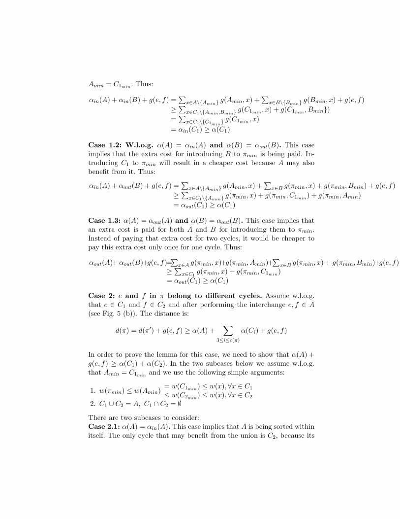
Amin = C1min . Thus:

αin(A) + αin(B) + g(e, f) =∑

x∈A\{Amin} g(Amin, x) +∑

x∈B\{Bmin} g(Bmin, x) + g(e, f)≥∑

x∈C1\{Amin,Bmin} g(C1min , x) + g(C1min , Bmin})=∑

x∈C1\{C1min} g(C1min , x)

= αin(C1) ≥ α(C1)

Case 1.2: W.l.o.g. α(A) = αin(A) and α(B) = αout(B). This caseimplies that the extra cost for introducing B to πmin is being paid. In-troducing C1 to πmin will result in a cheaper cost because A may alsobenefit from it. Thus:

αin(A) + αout(B) + g(e, f) =∑

x∈A\{Amin} g(Amin, x) +∑

x∈B g(πmin, x) + g(πmin, Bmin) + g(e, f)≥∑

x∈C1\{Amin} g(πmin, x) + g(πmin, C1min) + g(πmin, Amin)= αout(C1) ≥ α(C1)

Case 1.3: α(A) = αout(A) and α(B) = αout(B). This case implies thatan extra cost is paid for both A and B for introducing them to πmin.Instead of paying that extra cost for two cycles, it would be cheaper topay this extra cost only once for one cycle. Thus:

αout(A)+ αout(B)+g(e, f)=∑

x∈A g(πmin, x)+g(πmin, Amin)+∑

x∈B g(πmin, x) + g(πmin, Bmin)+g(e, f)≥∑

x∈C1g(πmin, x) + g(πmin, C1min)

= αout(C1) ≥ α(C1)

Case 2: e and f in π belong to different cycles. Assume w.l.o.g.that e ∈ C1 and f ∈ C2 and after performing the interchange e, f ∈ A(see Fig. 5 (b)). The distance is:

d(π) = d(π′) + g(e, f) ≥ α(A) +∑

3≤i≤c(π)

α(Ci) + g(e, f)

In order to prove the lemma for this case, we need to show that α(A) +g(e, f) ≥ α(C1) + α(C2). In the two subcases below we assume w.l.o.g.that Amin = C1min and we use the following simple arguments:

1. w(πmin) ≤ w(Amin)= w(C1min) ≤ w(x), ∀x ∈ C1

≤ w(C2min) ≤ w(x), ∀x ∈ C2

2. C1 ∪ C2 = A, C1 ∩ C2 = ∅

There are two subcases to consider:Case 2.1: α(A) = αin(A). This case implies that A is being sorted withinitself. The only cycle that may benefit from the union is C2, because its

minimum cost element, C2min , might be more expensive than C1min =Amin. Since C1min may be more expensive than πmin, C2 may benefitmore from uniting with the cycle of πmin. Thus:

αin(A) + g(e, f) =∑

x∈A\{Amin} g(Amin, x) + g(e, f)≥∑

x∈C1\{C1min} g(C1min , x) +

∑x∈C2

g(πmin, x) + g(πmin, C2min)= αin(C1) + αout(C2) ≥ α(C1) + α(C2)

Case 2.2: α(A) = αout(A). This case implies that the extra cost forintroducing A to πmin is being paid. There are two interchanges performedhere, which result in uniting the cycles C1 and C2 with the cycle of πmin.These two operations cost us exactly g(Amin, πmin) + g(e, f). However,the same result can be achieved with perhaps a cheaper cost (but nevermore expensive). Simply unite C1 with the cycle of πmin and C2 with thecycle of πmin separately. This will cost g(C1min , πmin) + g(C2min , πmin)and may only be cheaper. Thus:

αout(A) + g(e, f) =∑

x∈A g(πmin, x) + g(πmin, Amin) + g(e, f)≥∑

x∈C1g(πmin, x) +

∑x∈C2

g(πmin, x) + g(πmin, C1min) + g(πmin, C2min)= αout(C1) + αout(C2) ≥ α(C1) + α(C2)

ut

Theorem 1 immediately follows from the upper bound of the algorithmand Lemma 1.

Theorem 1. Let π be a permutation string and let C1, . . . , Cc(π) be thecycles of Gπ. Then the minimum cost for sorting π by interchanges underECM for any general function is:

d(π) =∑

1≤i≤c(π)

α(Ci).

Complexity: By Theorem 1, the CEAps algorithm computes the distanced(π). Computing the permutation cycles can be done in linear time by aleft to right traversal. Also, testing all the cycles is done in linear time,since the first element e in the adjacency list of Cimin (or πmin) can betaken in O(1) time. The interchange (e, Cimin) (resp. (e, πmin)) then sortse and the original cycle is shortened by one element, but Cimin (or πmin)are still in the cycle, so this process can be repeated until all elements inthe cycle are sorted. Therefore, the CEAps algorithm runs in linear time.

4 Rearranging General Strings

In the previous section we showed a linear time algorithm that computesthe distance in the interchange rearrangement problem when the inputstring is a permutation string and for every general function. In this sec-tion we consider the following problem:

Definition 5. Let S be the input string and T be the target string, whenS is a permutation of T and let g : Σ × Σ → R+ be a general function.Compute the minimum cost for transforming S into T by interchangeswhen the cost of interchanging elements x and y is defined by g(x, y).

The interchange rearrangement problem under the UCM for generalstrings is NP-hard [4]. Hence, as the UCM is a special case of ECMwhere all elements have equal weights, Corollary 1 follows:

Corollary 1. The interchange rearrangement problem under ECM forgeneral strings is NP-hard.

In the following subsection we present an O(n) time, 3-approximationalgorithm for any general function. In addition, we present an O(n·lg |Σ|)time 1.72-approximation algorithm for the summation function.

4.1 O(n) time 3-approximation algorithm for generalfunctions

The hardness of this problem is due to the difficulty of pairing each ele-ment in S with an identical element in T (converting the problem into apermutation string problem) in a way that gives the minimum distance.As explained in Section 2, pairing elements from S with elements in Tis equivalent to performing an edge-disjoint decomposition of GS,T intodirected cycles. Since S is a permutation of T , each of the strongly con-nected components the graph graph GS,T is an Eulerian directed graphand such a decomposition exists. The CEAgs algorithm (Fig. 6) arbitrar-ily decomposes GS,T into cycles and then applies the CEAps algorithm(Fig. 4). We prove the following theorem:

Theorem 2. The CEAgs algorithm gives a 3-approximation ratio forany general function.

Proof. We first observe that any solution for the problem implies a de-composition of GS,T into edge-disjoint directed cycles. This is true be-cause any solution implies a pairing of the elements of S and T , which is

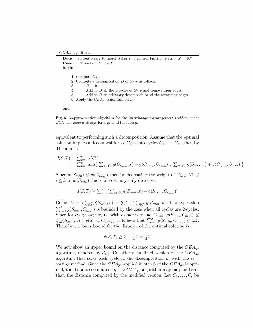
CEAgs algorithm.

Data : Input string S, target string T , a general function g : Σ ×Σ → R+

Result : Transform S into Tbegin

1. Compute GS,T .2. Compute a decomposition D of GS,T as follows:3. D ← ∅.4. Add to D all the 1-cycles of GS,T and remove their edges.5. Add to D an arbitrary decomposition of the remaining edges.6. Apply the CEAps algorithm on D.

end

Fig. 6. 3-approximation algorithm for the interchange rearrangement problem underECM for general strings for a general function g.

equivalent to performing such a decomposition. Assume that the optimalsolution implies a decomposition of GS,T into cycles C1, . . . , Ck. Then byTheorem 1:

d(S, T ) =∑k

i=1 α(Ci)=∑k

i=1 min{∑

x∈Ci g(Cimin , x)− g(Cimin , Cimin) ,∑

x∈Ci g(Smin, x) + g(Cimin , Smin) }

Since w(Smin) ≤ w(Cimin) then by decreasing the weight of Cimin ,∀1 ≤i ≤ k to w(Smin) the total cost may only decrease:

d(S, T ) ≥∑k

i=1(∑

x∈Ci g(Smin, x)− g(Smin, Cimin))

Define Z =∑

x∈S̃ g(Smin, x) =∑k

i=1

∑x∈Ci g(Smin, x). The expression∑k

i=1 g(Smin, Cimin) is bounded by the case when all cycles are 2-cycles.Since for every 2-cycle, C, with elements x and Cmin: g(Smin, Cmin) ≤12(g(Smin, x) + g(Smin, Cmin)), it follows that

∑ki=1 g(Smin, Cimin) ≤ 1

2Z.Therefore, a lower bound for the distance of the optimal solution is:

d(S, T ) ≥ Z − 12Z = 1

2Z

We now show an upper bound on the distance computed by the CEAgsalgorithm, denoted by dalg. Consider a modified version of the CEAgsalgorithm that sorts each cycle in the decomposition D with the αoutsorting method. Since the CEAps applied in step 6 of the CEAgs is opti-mal, the distance computed by the CEAgs algorithm may only be lowerthan the distance computed by the modified version. Let C1, . . . , Cl be

the cycles arbitrarily decomposed by the CEAgs algorithm. We thereforehave:

dalg ≤∑l

i=1(∑

x∈Ci g(Smin, x) + g(Smin, Cimin))≤ Z + 1

2Z = 112Z

The ratio between dalg and d(S, T ) is: dalgd(S,T ) ≤

1 12Z

12Z

= 3. ut

Complexity: Since a GS,T computation and an arbitrary decompositionof GS,T can be computed in linear time and since the CEAps algorithmis a linear time algorithm, the CEAgs algorithm runs in linear time.

4.2 O(n · lg |Σ|) time 1.72-approximation algorithm for thesummation function

In this subsection we consider the special case of the summation function,i.e, g(x, y) = w(x) + w(y). The αin(C), αout(C) for a given cycle aretherefore defined as follows:

• αin(C) =∑

x∈C\{Cmin} g(Cmin, x) =∑

x∈C w(x) + (|C| − 2) ·w(Cmin)• αout(C) =

∑x∈C g(Smin, x) + g(Smin, Cmin) =

∑x∈C w(x) + (|C| +

1) · w(Smin) + w(Cmin)

We show that applying the CEAps algorithm on the decomposition pre-sented by [4] gives a 1.72-approximation ratio. The decomposition pre-sented by [4] is basically the same as the decomposition of the CAEgsexcept that it contains a maximum number of 2-cycles. This difference isrepresented by step 5 of the CAE+

gs (Fig. 7). We use the following lemma,proved by [4]:

Lemma 2. [4] Given an Eulerian directed graph G = (V,E), then forevery 2-cycle, C, in G there exists a decomposition of E into a maximumnumber of edge-disjoint directed cycles, in which C appears as a cycle inthe decomposition.

By Lemma 2 there exists a decomposition of GS,T into a maximum num-ber of edge-disjoint directed cycles that contains a maximum number of2-cycles. This can be shown inductively by repeatedly finding a 2-cycleand removing it from GS,T until there are no more 2-cycles. By Lemma 2in every stage, there exists a decomposition into a maximum number ofedge-disjoint directed cycles that contains the chosen 2-cycle. Removingit results in a new graph G′, for which all its strongly connected compo-nents are Eulerian directed graphs. Therefore, the same can be appliedfor G′. We prove the following theorem:

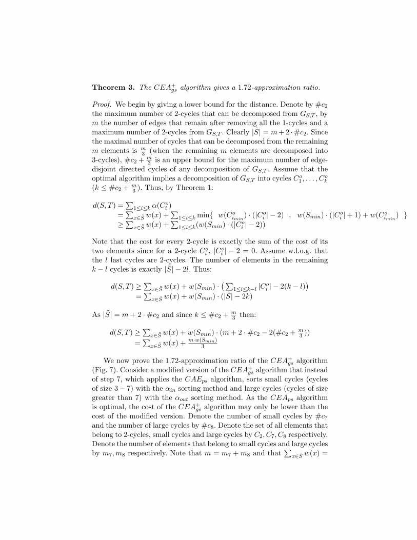
Theorem 3. The CEA+gs algorithm gives a 1.72-approximation ratio.

Proof. We begin by giving a lower bound for the distance. Denote by #c2the maximum number of 2-cycles that can be decomposed from GS,T , bym the number of edges that remain after removing all the 1-cycles and amaximum number of 2-cycles from GS,T . Clearly |S̃| = m+ 2 ·#c2. Sincethe maximal number of cycles that can be decomposed from the remainingm elements is m

3 (when the remaining m elements are decomposed into3-cycles), #c2 + m

3 is an upper bound for the maximum number of edge-disjoint directed cycles of any decomposition of GS,T . Assume that theoptimal algorithm implies a decomposition of GS,T into cycles Co1 , . . . , C

ok

(k ≤ #c2 + m3 ). Thus, by Theorem 1:

d(S, T ) =∑

1≤i≤k α(Coi )=∑

x∈S̃ w(x) +∑

1≤i≤k min{ w(Coimin) · (|Coi | − 2) , w(Smin) · (|Coi |+ 1) + w(Coimin) }≥∑

x∈S̃ w(x) +∑

1≤i≤k(w(Smin) · (|Coi | − 2))

Note that the cost for every 2-cycle is exactly the sum of the cost of itstwo elements since for a 2-cycle Coi , |Coi | − 2 = 0. Assume w.l.o.g. thatthe l last cycles are 2-cycles. The number of elements in the remainingk − l cycles is exactly |S̃| − 2l. Thus:

d(S, T ) ≥∑

x∈S̃ w(x) + w(Smin) ·(∑

1≤i≤k−l |Coi | − 2(k − l))

=∑

x∈S̃ w(x) + w(Smin) · (|S̃| − 2k)

As |S̃| = m+ 2 ·#c2 and since k ≤ #c2 + m3 then:

d(S, T ) ≥∑

x∈S̃ w(x) + w(Smin) · (m+ 2 ·#c2 − 2(#c2 + m3 ))

=∑

x∈S̃ w(x) + m·w(Smin)3

We now prove the 1.72-approximation ratio of the CEA+gs algorithm

(Fig. 7). Consider a modified version of the CEA+gs algorithm that instead

of step 7, which applies the CAEps algorithm, sorts small cycles (cyclesof size 3− 7) with the αin sorting method and large cycles (cycles of sizegreater than 7) with the αout sorting method. As the CEAps algorithmis optimal, the cost of the CEA+

gs algorithm may only be lower than thecost of the modified version. Denote the number of small cycles by #c7and the number of large cycles by #c8. Denote the set of all elements thatbelong to 2-cycles, small cycles and large cycles by C2, C7, C8 respectively.Denote the number of elements that belong to small cycles and large cyclesby m7,m8 respectively. Note that m = m7 + m8 and that

∑x∈S̃ w(x) =

CEA+gs algorithm.

Data : Input string S, target string TResult : Transform S into Tbegin

1. Compute GS,T .2. Compute a decomposition D of GS,T as follows:3. D ← ∅.4. Add to D all the 1-cycles of GS,T and remove their edges.5. Add to D a maximum number of 2-cycles from GS,T and remove their edges.6. Add to D an arbitrary decomposition of the remaining edges.7. Apply the CEAps algorithm on D.

end

Fig. 7. 1.72-Approximation algorithm for the interchange rearrangement problem un-der ECM for general strings for the summation function.

∑x∈C2

w(x)+∑

x∈C7w(x)+

∑x∈C8

w(x). The lower bound of the problemcan be rewritten as:∑x∈S̃

w(x)+m · w(Smin)

3=∑x∈C2

w(x)︸ ︷︷ ︸a

+∑x∈C7

w(x) +m7

3· w(Smin)︸ ︷︷ ︸

b

+∑x∈C8

w(x) +m8

3· w(Smin)︸ ︷︷ ︸

c

The CEA+gs algorithm pays exactly the cost for invariant a. We now

analyze the cost for invariants b and c. We use the following arguments:

1. For a cycle Ci: w(Cimin) ≤∑x∈Ci

w(x)

|Ci|2. #c8 ≤ m8

83.∑

x∈C8w(x) ≥ m8 · w(Smin)

4. ∀x, y, z ≥ 0: x+yx+z ≥ 1 and 0 ≤ x′ ≤ x ⇒ x+y

x+z ≤x′+yx′+z

Denote by balg the cost for sorting all the small cycles (using αin). Assumethat the small cycles are Cs1 , . . . , C

s#c7

Using argument 1, balg is boundedby:

balg =∑x∈C7

w(x) +∑

1≤i≤#c7

w(Csimin) · |Csi | − 2 ≤ 157

∑x∈C7

w(x)

The ratio between balg and invariant b is:

balgb≤

157

∑x∈C7

w(x)∑x∈C7

w(x) + m73 · w(Smin)

≤ 157≤ 1.72

Denote by calg the cost for sorting all the large cycles (using αout). Assumethat the large cycles are C l1, . . . , C

l#c8

. Using arguments 1, 2, 3, calg isbounded by:

calg =∑

x∈C8w(x) + w(Smin) ·

∑1≤i≤#c8

(|C li |+ 1) +∑

1≤i≤#c8w(C limin)

=∑

x∈C8w(x) + w(Smin) ·m8 + w(Smin) ·#c8 +

∑1≤i≤#c8

w(C limin)≤ 11

8

∑x∈C8

w(x) + 118m8 · w(Smin)

Using arguments 3 and 4, the ratio between calg and c is:

calgc ≤

1 18

∑x∈C8

w(x)+1 18m8·w(Smin)∑

x∈C8w(x)+

m83·w(Smin)

=18

∑x∈C8

w(x)∑x∈C8

w(x)+m83·w(Smin)

+∑x∈C8

w(x)+1 18m8·w(Smin)∑

x∈C8w(x)+

m83·w(Smin)

≤ 18 + m8·w(Smin)+1 1

8m8·w(Smin)

m8·w(Smin)+m83·w(Smin)

≤ 18 + 2 1

8

1 13

≤ 1.72

Therefore,

dalg ≤ aalg + balg + calg ≤ 1.72 · (a+ b+ c) ≤ 1.72 · d(S, T )

ut

Complexity: The CEA+gs algorithm differs from the CEAgs algorithm

only in step 5 of CEA+gs. Finding a maximum number of 2-cycles in GS,T

can be done in O(n · lg(|Σ|)) time in the following way. For each edge (oftotal n edges) in the graph check if there exists an edge in the oppositedirection. Since there are |Σ| nodes and the nodes can be kept orderedin the adjacency lists, this check can be done in O(log |Σ|) time for eachedge. As a corollary of Lemma 2 repeatedly finding and removing 2-cyclesthis way gives a maximum number of 2-cycles. Therefore, the CEA+

gs

algorithm runs in O(n · lg(|Σ|)) time.

5 The Transposition Rearrangement Problem

In this section we briefly discuss the transposition rearrangement problemin order to have a broadened view on the cost models. We refer to a singleelement transposition and not to a block transposition as referred to in [6]and [11]. We define the transposition operator as follows:

Definition 6. Let S = s1, . . . , sn be a string. A transposition of an el-ement si, ` positions forward transforms the string S into the stringS′ = s1, . . . , si−1, si+1, . . . , si+`, si, si+`+1, . . . , sn and a transposition ofan element si, ` positions backward transforms the string S into the stringS′ = s1, . . . , si−`−1, si, si−`, . . . , si−1, si+1, . . . , sn.

Subsection 5.1 considers the problem under the UCM and under the ECMfor both permutation strings and general strings. Subsection 5.2 considersthe problem under the LCM.

5.1 Element-Cost and Unit-Cost Models

In this subsection the following problem is discussed:

Definition 7. Let S be the input string and T be the target string andlet w : Σ → R+ be a weight function. Compute the minimum cost fortransforming S into T by transpositions when the cost of transposing anelement x is defined by w(x).

This definition generalizes all the sub-problems presented in Table 2. IfS is a permutation string, π, the problem is to sort π at minimum cost.If ∀x, y ∈ Σ, w(x) = w(y), the problem is to transform S into T with aminimum number of transpositions, i.e, UCM. For this set of problems,we use the following lemma:

Lemma 3. In the transposition rearrangement problem under UCM orunder ECM, each element is transposed at most once.

Proof. Assume to the contrary that there exists an optimal solution OPT ,such that dOPT = d(S, T ) and OPT transposes an element x (w(x) > 0)more than once. Consider the solution OPT ′ that applies all OPT trans-positions except for those applied on x and finally transposes x once toits position. Therefore, dOPT ′ < dOPT in contradiction to the minimalityof dOPT . ut

Lemma 3 implies that in the optimal solution for the problems definedin this subsection the elements of S are divided into two sets: the set A ofelements that are transposed exactly once and the set B of elements thatare not transposed at all. Therefore, the distance is defined as follows:

d(S, T ) =∑x∈A

w(x) =∑x∈S

w(x)−∑x∈B

w(x)

Since B contains elements that are not transposed at all, these elementsconstruct a common subsequence of S and T . Since d(S, T ) is minimizedwhen

∑x∈B w(x) is maximized, B is a common subsequence of highest

cost. The details for the various problems are presented in Table 2. TheMeasure column indicates the relevant subsequence of the specific prob-lem.

5.2 Length-Cost Model

In the interchange rearrangement problem under the LCM presentedin [4], the cost of every operation was defined by applying a length func-tion to the interchange length. They considered the f(`) = `α length func-tions for every α. In this section we discuss only the case where α = 1 (the

Table 2. Transposition rearrangement problem under UCM and ECM

Cost String Measure Description Distance∗ TimeModel Type Complexity

Permutation LIS Longest Increasing n− LIS(π) [14] O(n lgn)UCM String Subsequence

General LCS Longest Common n− LCS(S, T ) O(n2)String Subsequence

Permutation MWIS Maximum Weighted∑ni=1 w(πi)−MWIS(π) O(n lgn)

ECM String IncreasingSubsequence

General MWCS Maximum Weighted∑ni=1 w(si)−MWCS(S, T ) O(n2)

String CommonSubsequence

∗ LIS and LCS refer to the size of the subsequence. MWIS and MWCS refer to thesum of the weights of the subsequence’s elements.

case where α > 1 implies only transpositions of size 1 as shown below forα = 1, and is, therefore, the same). We consider the following problem:

Definition 8. Let S be the input string and T be the target string. Com-pute the minimum cost for transforming S into T by transpositions whenthe cost of transposing an element ` positions is `.

Permutation Strings. In this case, the input is a permutation stringπ and the problem is to sort π at a minimum cost. Given a permutationstring π, we say that πi and πj are reversed iff i < j and πi > πj . Let Rπ

be the set of pairs {i, j}, such that πi and πj are reversed. For example,in the string: S = D,A,C,B, we have Rπ = {{1, 2}, {1, 3}, {1, 4}, {3, 4}}.Lemma 4. Let π be a permutation string. Then the cost for sorting π bytranspositions under LCM is d(π) = |Rπ|.

Proof. A lower bound of the distance is |Rπ|, since for every reversed pair,{i, j}, 1-length unit must be paid (either πi must ”jump” over πj or viceversa), d(π) ≥ |Rπ|. This bound is achieved by a simple algorithm (sim-ilar to the max sort algorithm), which transposes the maximal elementto the rightmost position, then transposes the remaining elements fromthe maximum to the minimum, by transposing each element to the left ofthe previous transposed element. Since the transpositions are performedfrom the maximum element to the minimum element, every transposedelement only ”jumps” over elements that are reversed with it and, there-fore, d(π) ≤ |Rπ|. The lemma follows. ut

Complexity: Computing |Rπ| can be done in O(n lg n) time by using abalanced search tree supporting position queries.

General Strings. The difficulty for a general string input is to pair theelements of S with the elements of T in a way that gives the minimumcost. In the interchange rearrangement problem, this task is NP-hard.Here, however, an optimal pairing can be defined, as stated by Lemma 5(which can be easily verified).

Lemma 5. Let S be the input string and T be the target string. Let πobe the labeling that for any a ∈ Σ and k, labels the kth a in S as theposition of the kth a in T (πo pairs the kth a in S with the kth a in T ).Then the cost for transforming S into T by transpositions under LCM isd(S, T ) = d(πo).

Complexity: Since finding the labeling described in Lemma 5 can be donein O(n lg n), the total time complexity is O(n lg n).

References

1. A. Amir, Y. Aumann, G. Benson, A. Levy, O. Lipsky, E. Porat, S. Skiena, andU. Vishne. Pattern matching with address errors: Rearrangement distances. InProc. of the 17th annual ACM-SIAM Symposium on Discrete Algorithm (SODA),pages 1221–1229, 2006.

2. A. Amir, Y. Aumann, P. Indyk, A. Levy, and E. Porat. Efficient computations ofl1 and linfinity. In Proc. of the 14th International Symposium on String Processing

and Information Retrieval (SPIRE), pages 39–49, 2007.3. A. Amir, Y. Aumann, O. Kapah, A. Levy, and E. Porat. Approximate string

matching with address bit errors. In Proc. of the 19th Annual Symposium onCombinatorial Pattern Matching (CPM), pages 118–130, 2008.

4. A. Amir, T. Hartman, O. Kapah, A. Levy, and E. Porat. On the cost of interchangerearrangement in strings. In Proc. of the 15th Annual European Symposium onAlgorithms (ESA), pages 99–110, 2007.

5. S. Angelov, K. Kunal, and A. McGregor. Sorting and selection with random costs.In Proc. of the 8th Latin American Theoretical Informatics (LATIN), 2008.

6. V. Bafna and P. A. Pevzner. Sorting by transpositions. SIAM Journal on DiscreteMathematics, 11:224–240, May 1998.

7. P. Berman and S. Hannenhalli. Fast sorting by reversal. In Proc. 8th AnnualSymposium on Combinatorial Pattern Matching (CPM), volume 1075, pages 168–185, 1996.

8. A. Carpara. Sorting by reversals is difficult. In Proc. 1st Annual Intl. Conf. onResearch in Computational Biology (RECOMB), pages 75–83, 1997.

9. A. Cayley. Note on the theory of permutations. Philosophical Magazine, (34):527–529, 1849.

10. D. A. Christie. Sorting by block-interchanges. Information Processing Letters,60:165–169, 1996.

11. I. Elias and T. Hartman. A 1.375-approximation algorithm for sorting by transposi-tions. In Proc. of the 5th International Workshop on Algorithms in Bioinformatics(WABI), pages 204–214, 2005.

12. A. Gupta and A. Kumar. Sorting and selection with structured costs. In Proc. ofthe 42nd Symposium on Foundations of Computer Science, pages 416–425, 2001.

13. D. Gusfield. Algorithms on Strings, Trees, and Sequences: Computer Science andComputational Biology. Cambridge University Press, 1997.

14. L. S. Heath and J. P. C. Vergara. Sorting by bounded block-moves. DiscreteApplied Mathematics, 88(1-3):181–206, 1998.

15. L. S. Heath and J. P. C. Vergara. Sorting by short swaps. Journal of ComputationalBiology, 10(5):775–789, 2003.