intercalibrated passive microwave rain products from the

Intercalibrated Passive Microwave Rain Products from the Unified Microwave OceanRetrieval Algorithm (UMORA)

K. A. HILBURN AND F. J. WENTZ

Remote Sensing Systems, Santa Rosa, California

(Manuscript received 1 November 2006, in final form 12 July 2007)

ABSTRACT

The Unified Microwave Ocean Retrieval Algorithm (UMORA) simultaneously retrieves sea surfacetemperature, surface wind speed, columnar water vapor, columnar cloud water, and surface rain rate froma variety of passive microwave radiometers including the Special Sensor Microwave Imager (SSM/I), theTropical Rainfall Measuring Mission (TRMM) Microwave Imager (TMI), and the Advanced MicrowaveScanning Radiometer for Earth Observing System (AMSR-E). The rain component of UMORA explicitlyparameterizes the three physical processes governing passive microwave rain retrievals: the beamfillingeffect, cloud and rainwater partitioning, and effective rain layer thickness. Rain retrievals from the previousversion of UMORA disagreed among different sensors and were too high in the tropics. These issues havebeen fixed with more realistic rain column heights and proper modeling of saturation and footprint-resolution effects in the beamfilling correction. The purpose of this paper is to describe the rain algorithmand its recent improvements and to compare UMORA retrievals with Goddard Profiling Algorithm(GPROF) and Global Precipitation Climatology Project (GPCP) rain rates. On average, TMI retrievalsfrom UMORA agree well with GPROF; however, large differences become apparent when the instanta-neous retrievals are compared on a pixel-to-pixel basis. The differences are due to fundamental algorithmdifferences. For example, UMORA generally retrieves higher total liquid water, but GPROF retrieves ahigher surface rain rate for a given amount of total liquid water because of differences in microphysicalassumptions. Comparison of UMORA SSM/I retrievals with GPCP shows similar spatial patterns, butGPCP has higher global averages because of greater amounts of precipitation in the extratropics. UMORAand GPCP have similar linear trends over the period 1988–2005 with similar spatial patterns.

1. Introduction

The Unified Microwave Ocean Retrieval Algorithm(UMORA) simultaneously retrieves sea surface tem-perature, surface wind speed, columnar water vapor,columnar cloud water, and surface rain rate from a va-riety of passive microwave sensors including SpecialSensor Microwave Imager (SSM/I), Tropical RainfallMeasuring Mission (TRMM) Microwave Imager(TMI), and the Advanced Microwave Scanning Radi-ometer (AMSR) (Wentz 1997; Wentz and Spencer1998; Wentz and Meissner 2000). The products areavailable on quarter-degree grids in easy-to-use binaryfile formats with complete documentation and readcode at our Web site (http://www.remss.com). The rainretrieval component of the algorithm was developed by

Wentz and Spencer (1998, hereinafter WS98). Thephysical basis for the algorithm is that dual-polarizationpassive microwave measurements provide an accurateestimate of �2—the two-way transmittance through theatmosphere. The three physical processes governingthe retrieval of surface rain rate from �2 are 1) varyingrain intensities across the radiometer footprint (the“beamfilling effect”); 2) the relative partitioning ofcloud and rainwater, which depends in part upon therain drop size distribution; and 3) the effective rainlayer thickness (“effective” because of the nonuniformvertical distribution of rainwater). UMORA isolatesthese processes so it is possible to change them and assesstheir impact on retrieved rain rates. Thus, we can findphysical explanations for discrepancies in our retrievals.

In addition to the retrieval algorithm, the other criti-cal component to obtaining accurate rain retrievals isthe radiometer calibration at the brightness tempera-ture (TB) level. Remote Sensing Systems (RSS) hasspent much effort intercalibrating satellite microwave

Corresponding author address: Kyle Hilburn, Remote SensingSystems, 438 First Street, Suite 200, Santa Rosa, CA 95401.E-mail: [email protected]

778 J O U R N A L O F A P P L I E D M E T E O R O L O G Y A N D C L I M A T O L O G Y VOLUME 47

DOI: 10.1175/2007JAMC1635.1

© 2008 American Meteorological Society

JAMC1635

radiometers, starting with SSM/I in 1987. In the mostrecent version 6, the six SSM/Is have been carefullyintercalibrated to a precision of about 0.1 K in TB, andTMI and the AMSR for Earth Observing System(EOS) (AMSR-E) have been adjusted to match theSSM/I time series. The success of this intercalibrationeffort can be seen in the excellent agreement of colum-nar water vapor retrievals shown in Fig. 1. Also, trendsin the SSM/I wind speed retrievals now agree with buoytrends to an accuracy of 0.1 m s�1 decade�1. Windspeed retrievals are very sensitive to TB calibration er-rors, and the good agreement with buoys indicates anintercalibration error of 0.1–0.2 K or less.

Despite the good TB calibration, the rain retrievalsfrom different sensors did not agree (Fig. 1). The WS98rain-rate retrievals had two major problems: 1) the rainrates were too high in the tropics and 2) the retrievalsfrom different sensors did not agree. The first problemwas due to the use of inappropriate rain columnheights. The second problem was due to the failure toinclude the different resolutions of the sensors (Table1) in the beamfilling correction. The purpose of thispaper is to communicate what has been found in solvingthese two problems. The answers are not just specific toour algorithm, but have broader applicability to passivemicrowave rain retrievals. It turns out that other pas-sive microwave rain retrieval algorithms also have in-tersatellite differences, and removing these artifacts is amajor goal of the Global Precipitation Measurement(GPM) mission.

There are two motivations for this paper. The first isto explain the improvements we have made to theWS98 rain algorithm focusing especially on those thataddress the intersatellite differences. The second moti-vation is to compare our rain products against otherrain products. The goal of this comparison is not toassert that one product is necessarily better than an-other; but to 1) assess the level of agreement/disagree-ment that exists and any patterns in the disagreement,

2) examine the microphysical assumptions in our algo-rithm in comparison with other algorithms to see whatrole they play in retrieval differences, and 3) to assesslong-term trends in the various datasets and comparetheir consistency. In section 2, we describe theUMORA datasets and the other datasets that we usedin this study. In section 3, we describe the rain algo-rithm and explain changes made to beamfilling (section3a), cloud and rain partitioning (section 3b), and effec-tive rain layer thickness (section 3c). In section 4 wecompare TMI retrievals from UMORA and GPROF toassess their agreement both on average and for instan-taneous pixel-to-pixel comparisons. We also examinethe consistency of UMORA SSM/I rain retrievals andassess the impact of the diurnal cycle on different SSM/I. Finally, we compare means and trends in UMORASSM/I rain retrievals with GPCP rain rates.

2. Data

We have intercalibrated the SSM/I (F08, F10, F11,F13, F14, and F15), TMI, and AMSR-E instrumentsand processed the data with the improved UMORAalgorithm. The new data are: version 6 SSM/I, version 4TMI, and version 5 AMSR-E. The SSM/I provide dailyglobal coverage from July 1987 to the present, TMIprovides daily tropical coverage from December 1998

TABLE 1. The geometric average 3-dB footprint sizes for thechannels used by the UMORA rain algorithm for SSM/I, TMI(pre/post boost), and AMSR-E.

Sensor Frequency (GHz) Avg footprint size (km)

SSM/I 19.35 5637.0 32

TMI 19.35 24/2837.0 13/15

AMSR-E 18.7 2136.5 12

FIG. 1. (left) Zonal average water vapor, (middle) Wentz and Spencer rain rates, and (right) UMORA rain ratesfor the year 2003. Shown are data from F13 (green), F14 (blue), F15 (purple), AMSR-E (orange), and TMI (darkred). GPCP rain rates are shown for reference (black). Only ocean pixels are considered.

MARCH 2008 H I L B U R N A N D W E N T Z 779

Fig 1 live 4/C

to the present, and AMSR-E provides daily global cov-erage from June 2002 to the present. Retrievals aredone only over the ocean.

Our comparison data include the version 2 GlobalPrecipitation Climatology Project (GPCP) rain rates(Adler et al. 2003) and both the swath level (2A12) andgridded (3A12) version 6 Goddard Profiling Algorithm(GPROF) surface rain rates (Kummerow et al. 2001).The comparison of our TMI swath data with theGPROF swath data is unique because it is a pixel-to-pixel matchup between retrievals from the same sensoron the same satellite. Thus, the differences we findshould be almost entirely due to differences betweenthe UMORA and GPROF rain algorithms. It should benoted that we have performed our own independentcalibration of TMI (Wentz et al. 2001); however, thisshould be a small source of discrepancy betweenUMORA and GRPOF rain rates.

We used several sources of data in our estimation ofthe effective rain layer thickness. We used the radio-sonde dataset described in Wentz (1997) and WS98. Wealso make use of the National Centers for Environmen-tal Prediction (NCEP) Global Data Assimilation Sys-tem (GDAS) 0° isotherm height analysis. Our climato-logical SST product is the National Oceanic and Atmo-spheric Administration (NOAA)/NCEP Reynoldsoptimal interpolation (OI) version 2 SST (Reynolds etal. 2002). We also compared our heights with the Inter-national Telecommunication Union recommended rainheights (International Telecommunication Union2001).

3. Algorithm

The brightness temperature at the top of the atmo-sphere as seen by a satellite radiometer is expressed asthe sum of the upwelling atmospheric radiation, down-welling atmospheric radiation that is reflected upwardby the sea surface, and the direct emission of the seasurface attenuated by the intervening atmosphere. Thiscan be expressed as follows:

F � TBU � � �ETS � �1 � E��TBD � �TBC��, �1�

where TBU and TBD are the upwelling and downwellingatmospheric brightness temperatures and � is the trans-mittance through the atmosphere, E is the sea surfaceemissivity, TBC is the cosmic background radiation tem-perature of 2.7 K, and accounts for nonspecular re-flection. The upwelling and downwelling atmosphericbrightness temperatures are expressed in terms of ef-fective air temperatures TU and TD, defined by

TU � TBU��1 � �� and �2a�

TD � TBD��1 � ��. �2b�

In the nonraining case, there is no scattering, and theseeffective air temperatures are parameterized as func-tions of water vapor V and sea surface temperature TS

[i.e., TU � (V, TS) and TD � f(TU, V) as in Wentz(1997)]. In the raining case, scattering and rain-inducedvariations in air temperature make it necessary to makeTU a retrieved parameter. It is assumed that TD isclosely correlated with TU so that TD can be specified asa function of TU as in WS98. It is also assumed that TU

has the same value for vertical and horizontal polariza-tion. In the absence of scattering, TU is completely in-dependent of polarization. For moderate to heavy rain,TB observations show that saturation values for the ver-tical and horizontal polarization are nearly the same;making the assumption of polarization independenceseem reasonable. Thus, the retrieval problem is re-duced to solving two equations in two unknowns:

TBV � FV�TU, �2� and �3a�

TBH � FH�TU, �2�. �3b�

Thus, the physical basis for UMORA is the use of dual-polarization observations in order to separate the emis-sion signal (embodied by the two-way transmission: �2)from the scattering signal (embodied by the effectivetemperature depression: �TU � TU � ). Equations(3a) and (3b) are quadratic in � and linear in TU and caneasily be solved. To solve (3a) and (3b) we use theemissivity E and scattering models developed byWentz (1997) and updated by Meissner and Wentz(2002, 2004). Values for surface wind speed W and co-lumnar water vapor V used by the emissivity model areretrieved as in WS98. The emissivity model also re-quires values for sea surface temperature, which comefrom Reynolds OI version 2 SST (Reynolds et al. 2002);and surface wind direction, which comes from NCEPGDAS. The oxygen and vapor components of �2 arefactored out following WS98, thereby obtaining just thetwo-way liquid water transmittance �2

L.Equation (1) is complicated and obscures the essen-

tial physics of rain retrieval, so it is instructive to ex-amine a simplified form of (1). If we ignore the smalleffects of nonspecular reflection and the cosmic micro-wave background, and if we assume that the ocean–atmosphere system is isothermal with an effective tem-perature of TE, then we obtain a highly simplifiedmodel for brightness temperature:

TB � TE��1 � �2��, �4�


where � is the reflectivity of the sea surface (� � 1 � E).The effective temperature varies from the sea surfacetemperature to the effective temperature of the up-welling atmospheric radiation as the transmission goesfrom 1 to 0. We see that, through the use of vertical andhorizontal polarization measurements, TE can be elimi-nated and the two-way transmittance is given by

�2 �TBV � TBH

�HTBV � �VTBH. �5�

Examining (5), the solution to a simplified version of(1), we see that the essential physics of UMORA arethe same as Petty (1994). The advantage of such anapproach is that, as shown by Petty (1994), this tech-nique of separating emission and scattering providesaccurate estimates of transmittance even in the pres-ence of strong scattering by ice. Moreover, Spencer etal. (1989) show that ice makes a negligibly small ab-sorption contribution relative to that of liquid. Thus, wecan obtain reliable estimates of columnar liquid water(the total cloud plus rainwater) even in the presence ofscattering by ice.

This simplified model (5) also helps us see that thebasic observable for rain retrievals is �2, the footprint-averaged two-way transmittance, where (5) has beenevaluated with the footprint-average brightness tem-peratures. Consider, for example, a scene that has uni-form TS � 27°C, W � 7 m s�1, and V � 60 mm forSSM/I conditions (incidence angle of 53.4° and a fre-quency of 19.35 GHz). In this case we have �V � 0.424and �H � 0.716. Let us say that one-half of the footprintis rain free with TBV � 201 K and TBH � 138 K. Thereader can confirm that this implies � � 0.8589 and �2 �0.7377. Now let us say that the other one-half of thefootprint has heavy rain with TBV � 268 K and TBH �263 K. These values imply � � 0.2494 and �2 � 0.0622.Since brightness temperatures average in the usual lin-ear way, the whole footprint then has values of �TBV� �234.5 K and �TBH� � 200.5 K. The angle brackets � �denote averaging over the satellite footprint (i.e., theexpectation operator). Substituting these values into(5) gives �(�TB�) � 0.6405 and �2(�TB�) � 0.4102. Ifinstead we average the transmission values, we find that��(TB)� � 0.5542 and ��2(TB)� � 0.4000. In general, it istrue that

��2�TB�� 2��TB��, whereas �6a�

��TB�� TB��. �6b�

These facts are confirmed using the full radiative trans-fer model (1). This example shows that it is �2, not �,that is the basic observable.

Beamfilling enters the picture when estimating at-tenuation A from the two-way transmission �2. To beexplicit,

��2� � �etA� � etA � et�A�, A � �A� � A, �7�

where t � � 2 sec , A is the columnar attenuation, andA is the estimate of attenuation ignoring beamfilling[i.e., A � ln(�2)/t]. It is worth noting that (7) is simplya specific case of Jensen’s inequality and the left-handside of (7) is equivalent to the moment-generating func-tion of the subpixel attenuation probability distributionfunction. Our technique for estimating the beamfillingadjustment is described in section 3a.

Once an estimate of the two-way liquid water trans-mittance �2

L is obtained, there are three physical as-sumptions needed to retrieve the surface rain rate: thebeamfilling adjustment (section 3a), the relative parti-tioning of cloud and rainwater (section 3b), and the raincolumn height (section 3c). Please note that UMORAperforms the retrieval without using adjacent cell infor-mation: there is no smoothing, filtering, or analysis ofadjacent cell spatial variability.

It is worth noting that in the current version ofUMORA our parameterizations are “global.” That is,the same rain drop size distribution, rain–cloud thresh-old, and beamfilling parameterization are used every-where with no dependence on geographic location,time of year, time of day, ENSO phase, storm type [e.g.,ITCZ–southern Pacific convergence zone (SPCZ) con-vection, tropical cyclone, extratropical transition, extra-tropical cyclone], or rain type (e.g., convective or strati-form). The advantage of this simple strategy is that theparameterizations are more tightly constrained (i.e., theglobal average rain rate is bounded by what is hydro-logically possible). It is unrealistic, of course, to use aglobally constant value of effective rain layer thickness,and the parameterization must depend upon some geo-graphically and/or seasonally variable parameter. Thedifficulty is that, while passive microwave observationshave a strong liquid water attenuation signal, the infor-mation needed to convert total liquid water into surfacerain rate does not have a strong microwave signal. An-cillary data can be used to help specify these param-eterizations (as in our case for the effective rain layerthickness), but care must be taken that the ancillarydata do not introduce any spurious long-term trends.

The goal of this phase of algorithm development wasrelative calibration of the various radiometer rain re-trievals. The next step is an absolute calibration. In thenext phase of algorithm development, we plan to ex-amine the additional use of passive microwave scatter-


ing information for rain versus cloud thresholding. Hil-burn et al. (2006) have seen that passive microwavescattering information (�TU) may provide informationabout borderline cloud–rain cases, and in the nextphase of algorithm development we will examinewhether making the cloud–rain threshold a weak func-tion of scattering information will yield benefits. Wewill also examine the use of scattering and emissioninformation together for the discrimination of differentprecipitation types (e.g., convective and stratiform).This would allow us to choose different rain drop sizedistributions and scale the rain column height for moreappropriate values of effective rain layer thickness. Weplan to examine storm-scale rain structure (see section4) and use hydrological balance considerations (Wentzet al. 2007) to better constrain our assumptions. Thesemore complicated changes were not made at this timebecause of the importance of understanding the inter-satellite differences coming from our simple rain algo-rithm before adding additional complexity to the algo-rithm.

a. Beamfilling

The first step is to go from two-way liquid watertransmittance �2

L to liquid water columnar attenuationAL. This requires knowledge of the spatial distributionof liquid within the satellite footprint and is referred toas the “beamfilling effect.” The desired quantity is thefootprint-averaged attenuation

AL � �A�P�A�� dA�, �8�

where P(A�) is the probability distribution function forattenuation within the footprint. Instead, the measure-ment gives the footprint-averaged two-way transmit-tance

�L2 � � exp��2A� sec�P�A�� dA�. �9�

If the beamfilling were uniform, P(A�) would be thedelta function, and integrating (9) yields

�L2 � exp��2AL sec�. �10�

The estimate of attenuation ignoring beamfilling is

AL � �ln��L�

sec, �11�

and AL is called the “observed” attenuation because itis directly related to the fundamental measurement �2

as compared to the “true” attenuation, which is de-

noted by AL. The beamfilling correction multiplier isthen defined as

B �AL

AL

. �12�

If the beamfilling is nonuniform, then we need to as-sume some form for the spatial distribution of liquidwithin the footprint, P(A�), in order to calculate �2

L.Note that calculating �2

L is equivalent to evaluating themoment-generating function of A�L at � 2 sec . If weassume that P(A�) follows some two-parameter prob-ability distribution function (WS98 assume a gammadistribution), then the departure of the 19–37-GHz at-tenuation ratio from the theoretical Mie absorptiongives the variability of attenuation in the footprint.Thus, the physical basis for the beamfilling correction isthe use dual-frequency information to infer subpixelliquid water spatial variability.

The WS98 beamfilling correction had two problems.The first problem was that it did not explicitly accountfor the spatial resolution of the satellite observations.We find that the form of P(A�) changes systematicallyas a function of footprint size. WS98 assumed a distri-bution for P(A�) that works well for SSM/I resolutions(Table 1), but it assumes more spatial variability than isreally present in the smaller TMI and AMSR-E foot-prints. Thus the beamfilling overcorrected TMI andAMSR-E. We see that neglecting this resolution depen-dence in the beamfilling correction results in the rainretrievals from the higher-resolution sensors (AMSR-Eand TMI) being biased higher than SSM/I, as is shownby the WS98 results in Fig. 1. We also found that theTMI resampling routine was not working correctly forthe TMI maneuvers, causing TMI retrievals to be bi-ased even higher as a function of along-scan position.When this problem was fixed, the AMSR-E and TMIrain rates agreed, but were still high relative to SSM/Ibecause of the WS98 algorithm neglecting footprint-resolution effects. In the latest versions, the same re-sampling algorithm is now used for SSM/I, TMI, andAMSR-E in order to resample the brightness tempera-tures to a common set of spatial resolutions specific tothe sensor (Ashcroft and Wentz 2000). Thus, we pro-duce level 2 (i.e., swath level) rain rates at the resolu-tion of the 37-GHz footprint of the specific instrument(Table 1); however, all of our publicly available griddeddata are provided at 0.25° resolution.

The second problem with the WS98 beamfilling cor-rection was that it did not explicitly model saturation.The correction depends on the ratio of 37–19-GHz at-tenuations, but the response of the 37-GHz channelsaturates for lower rain rates than for 19 GHz, causing


spuriously large ratios. Hilburn et al. (2006) found thatthis caused the WS98 beamfilling correction to reach itsmaximum allowed values (B � 3.4 and 6.4 for the 19-and 37-GHz channels), which produced unrealisticstorm structure.

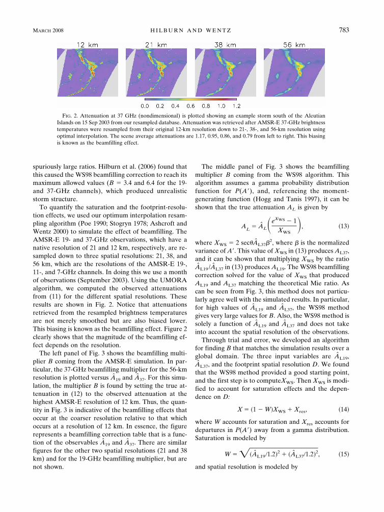
To quantify the saturation and the footprint-resolu-tion effects, we used our optimum interpolation resam-pling algorithm (Poe 1990; Stogryn 1978; Ashcroft andWentz 2000) to simulate the effect of beamfilling. TheAMSR-E 19- and 37-GHz observations, which have anative resolution of 21 and 12 km, respectively, are re-sampled down to three spatial resolutions: 21, 38, and56 km, which are the resolutions of the AMSR-E 19-,11-, and 7-GHz channels. In doing this we use a monthof observations (September 2003). Using the UMORAalgorithm, we computed the observed attenuationsfrom (11) for the different spatial resolutions. Theseresults are shown in Fig. 2. Notice that attenuationsretrieved from the resampled brightness temperaturesare not merely smoothed but are also biased lower.This biasing is known as the beamfilling effect. Figure 2clearly shows that the magnitude of the beamfilling ef-fect depends on the resolution.

The left panel of Fig. 3 shows the beamfilling multi-plier B coming from the AMSR-E simulation. In par-ticular, the 37-GHz beamfilling multiplier for the 56-kmresolution is plotted versus A19 and A37. For this simu-lation, the multiplier B is found by setting the true at-tenuation in (12) to the observed attenuation at thehighest AMSR-E resolution of 12 km. Thus, the quan-tity in Fig. 3 is indicative of the beamfilling effects thatoccur at the coarser resolution relative to that whichoccurs at a resolution of 12 km. In essence, the figurerepresents a beamfilling correction table that is a func-tion of the observables A19 and A37. There are similarfigures for the other two spatial resolutions (21 and 38km) and for the 19-GHz beamfilling multiplier, but arenot shown.

The middle panel of Fig. 3 shows the beamfillingmultiplier B coming from the WS98 algorithm. Thisalgorithm assumes a gamma probability distributionfunction for P(A�), and, referencing the moment-generating function (Hogg and Tanis 1997), it can beshown that the true attenuation AL is given by

AL � AL�eXWS � 1XWS

�, �13�

where XWS � 2 sec AL37�2, where � is the normalized

variance of A�. This value of XWS in (13) produces AL37,and it can be shown that multiplying XWS by the ratioAL19 /AL37 in (13) produces AL19. The WS98 beamfillingcorrection solved for the value of XWS that producedAL19 and AL37 matching the theoretical Mie ratio. Ascan be seen from Fig. 3, this method does not particu-larly agree well with the simulated results. In particular,for high values of AL19 and AL37, the WS98 methodgives very large values for B. Also, the WS98 method issolely a function of AL19 and AL37 and does not takeinto account the spatial resolution of the observations.

Through trial and error, we developed an algorithmfor finding B that matches the simulation results over aglobal domain. The three input variables are AL19,AL37, and the footprint spatial resolution D. We foundthat the WS98 method provided a good starting point,and the first step is to computeXWS. Then XWS is modi-fied to account for saturation effects and the depen-dence on D:

X � �1 � W�XWS � Xres, �14�

where W accounts for saturation and Xres accounts fordepartures in P(A�) away from a gamma distribution.Saturation is modeled by

W � ��AL19�1.2�2 � �AL37�1.2�2, �15�

and spatial resolution is modeled by

FIG. 2. Attenuation at 37 GHz (nondimensional) is plotted showing an example storm south of the AleutianIslands on 15 Sep 2003 from our resampled database. Attenuation was retrieved after AMSR-E 37-GHz brightnesstemperatures were resampled from their original 12-km resolution down to 21-, 38-, and 56-km resolution usingoptimal interpolation. The scene average attenuations are 1.17, 0.95, 0.86, and 0.79 from left to right. This biasingis known as the beamfilling effect.


Fig 2 live 4/C

Xres �D

120, �16�

where D is the footprint diameter in kilometers. In thealgorithm, we use the value of D associated with the19-GHz footprint, since that is the footprint size asso-ciated with the 19–37-GHz attenuation ratio. The valueof X coming from (14) is then substituted into (13) tofind the true attenuation. It should be emphasized that(14)–(16) represent an empirical fit to the beamfillingresults that come from the AMSR-E simulation. Theseresults represent global coefficients.

The right panel of Fig. 3 shows the new UMORAbeamfilling correction. It is clearly more representativeof the simulation results. It is small when the attenua-tions are near the theoretical Mie ratio and increases asthe actual ratio departs the Mie ratio. When the attenu-ation is large, greater than roughly 0.6, the beamfillingcorrection is small and does not depend as strongly onthe 19–37-GHz ratio. This behavior has also been ob-served by Varma et al. (2004), and is much differentthan assuming a pure gamma distribution for P(A�)(i.e., the WS98 assumption). Figure 4 shows AMSR-Erain rates for a particular storm using both the WS98and UMORA beamfilling correction. Saturation in thecenters of storms caused the WS98 beamfilling correc-tion to produce very high rain rates over unrealisticallylarge areas.

b. Cloud–rain partitioning

The second step in the rain retrieval is to go fromcolumnar liquid water attenuation AL to columnarcloud L and column-average rain rate R. The basicequations governing this are

AL19 � a19�1 � b19T�L � c19�1 � d19T�Re19H,

�17a�

AL37 � a37�1 � b37T�L � c37�1 � d37T�Re37H,

�17b�

T � TL � 283, and �17b�

TL � 251.5 � 0.83�TU � 240�, �17c�

where H is the height of the rain column, TL is the raincloud temperature, and TU � (V, TS). The values thatwe use for a, b, c, d, and e are given in Table 2. Thesecoefficients were derived using a Marshall–Palmer raindrop size distribution (see WS98 for more details) andcompare well to other accepted standards (e.g., Inter-national Telecommunication Union 1999). Note thatattenuation is linearly related to the columnar cloud

FIG. 4. This storm caught by AMSR-E in the North Atlantic on7 Sep 2003 is shown to illustrate the impact of properly modeledsaturation. Shown are (left) the WS98 rain rates and (right) theUMORA rain rates (mm h�1). Note the changes in the strength ofboth the center of the storm system and in the isolated showers.

FIG. 3. The multiplicative beamfilling correction factor B for 37 GHz is plotted to contrast (left) the AMSR simulated beamfillingcorrection, (middle) the WS98 beamfilling correction, and (right) the UMORA beamfilling correction. The theoretical Mie absorptionratio is shown for reference (solid line). Note that in the AMSR simulation as 37-GHz attenuation increases above 0.6, large departuresfrom the theoretical line do not imply large beamfilling correction factors. This is due to saturation, and the UMORA beamfillingcorrection more accurately models this effect.


Fig 3 4 live 4/C

water L, and weakly nonlinearly related to the column-average rain rate through the rain drop size distribu-tion. Changes in the drop size distribution will manifestthemselves through changes in the cloud and rainwaterpartitioning. Solving Eqs. (17a) and (17b) requires par-titioning the water between cloud and rain. Unfortu-nately, we have two equations but three unknowns. Inaddition, if we examine the ratios of the coefficients, wefind

a19

a37�

c19

c37, �18a�

and

e19 � e37 � 1. �18b�

This means that we cannot use dual-frequency mea-surements to reliably separate the cloud signal from therain signal or to estimate rain column height. Thus,while we have only one unique piece of information, wehave three unknowns. Based on a study of northeastPacific extratropical cyclones, WS98 choose a simplepartitioning relationship

L � ��1 � �HR�, �19�

where � � 0.18 mm. This relationship can be used tosolve (17a) and (17b) if we assume some value for H. Itis possible that the rain–cloud threshold � might de-pend on footprint size, and thus could explain discrep-ancies among sensors. We found that varying � maderelatively small changes in the average rain rate, but itmade very large changes in the rain coverage (Fig. 5).We concluded that globally adjusting the cloud–rainpartitioning threshold to obtain better agreement be-tween the various sensors is a bad option because itresulted in unrealistic rain coverage. We use the WS98value of 0.18 mm for UMORA. The reasonableness ofthis value is confirmed (in section 4) by comparingmaps of our fractional coverage with maps in Petty(1995).

c. Effective rain layer thickness

The third step of the retrieval is to prescribe a valuefor rain column height H. Doing so, we can solve (17a),

(17b), and (19) for the column-average rain rate, whichis given by

R � H�1�0

H

R�h� dh, �20�

where R(h) is the rain profile. The difference betweenthe column-average rain rate R and the surface rainrate R(0) is a source of error when comparing to in situsurface rain measurements. Ideally, we should use theeffective rain layer thickness Heff instead of the raincolumn height. The relationship between the effectiverain layer thickness Heff and the rain column height His given by

TABLE 2. Coefficients for our cloud and rain attenuation model.The top number is for SSM/I and TMI frequencies and the bottomnumber is for AMSR-E frequencies.

Frequency a b c d e

19 GHz 0.059 48 0.028 71 0.012 21 0.004 00 1.057 100.055 63 0.028 80 0.011 33 0.004 00 1.063 63

37 GHz 0.208 00 0.026 00 0.043 56 �0.002 00 0.951 860.202 71 0.026 08 0.042 49 �0.002 00 0.954 63

FIG. 5. (top) Zonal average rain rate and (bottom) fractionalrain coverage for one month of AMSR-E data where the cloud–rain threshold parameter has been varied from 0.05 to 0.30 mm(color bar). Our algorithm uses a typical value of 0.18 mm (heavyblack line) as a threshold. Note that modest changes in averagerain rate are associated with large changes in fractional rain cov-erage.


Fig 5 live 4/C

Heff � H� R

R�0��. �21�

The present version of UMORA assumes the samevalue as WS98: R/R(0) � 1, but in reality this ratio is astrong function of the microphysical and thermody-namic environment in which the rain is produced (e.g.,Liu and Fu 2001). While we recognize that a nonunityvalue for R/R(0) is probably more physically appropri-ate, this strong functionality makes it difficult for us toconfidently choose a value to be applied globally. Solv-ing (17a) and (17b) produces two estimates of the col-umn-average rain rate, one for the 19-GHz channel andone for the 37-GHz channel. We smoothly blend co-lumnar rain-rate estimates from the 37-GHz channel atlow values to the 19-GHz channel at high values.

WS98 used radiosonde observations to derive a rela-tionship between freezing level height and sea surfacetemperature (SST). They assume the rain columnheight is the same as the freezing level height. Theyfound that their expression gave rain rates that wereabout 3/5 smaller than climatology in the tropics. Theyfixed this discrepancy by forcing the rain column heightexpression to reach a maximum of 3 km in the tropics;much lower than the 5 km indicated by observations(Fig. 6). They acknowledged that this was a question-

able ad hoc correction. We now understand why thiscorrection was required. In computing the average forthe tropical rain, the WS98 algorithm excluded obser-vations having very large B. These cases occurred forless than roughly 10% of rain retrievals, and excludingthem had a much bigger effect on the average rain ratethan WS98 realized. These cases could occur at any rainrate, but formed the majority of rain retrievals greaterthan 5 mm h�1. Once these cases are included, the av-erage tropical rain increases by 5/3, and there is no needto apply the ad hoc correction to H, and the radio-sonde-derived relationship between H and SST can beused as is.

For UMORA, we took a closer look at the H versusSST relationship. We were concerned that the irregulargeographic sampling of the radiosonde observationsmight affect the regression, so we compared the radio-sonde observations against NCEP freezing level height(Fig. 6). They agree well in the tropics, disagree some-what where the radiosonde sampling is most incom-plete, and NCEP is slightly lower in the high latitudes.Figure 6 also shows that the International Telecommu-nication Union (ITU) recommended heights (Interna-tional Telecommunication Union 2001) agree withNCEP to within 0.5 km. We regressed NCEP freezinglevel heights against climatological sea surface tem-peratures, TSST, and found a simple linear relationshipfit well:

H � 0.46 � 0.16TSST, �22a�

H � 0.46, TSST � 0 C, and �22b�

H � 5.26, TSST � 30 C. �22c�

This is the relationship now used by UMORA.

4. Comparison

Our comparison consists of two separate activities.The first is to compare TMI rain retrievals fromUMORA to GPROF to see how they agree on average,to see how they agree instantaneously, to find reasonsfor disagreements especially related to microphysicalassumptions, and to assess long-term trends. The sec-ond activity is to examine SSM/I rain retrievals to seehow they agree among themselves, to see what impactthe diurnal cycle makes on SSM/I, and to see how wellmean and trends over the 18-yr period 1988–2005 com-pare in the UMORA SSM/I and GPCP datasets.

On average, UMORA and GPROF TMI rain re-trievals are very similar. Figure 7 compares averageTMI rain rates from UMORA and GPROF for thetime period 1998–2005. The UMORA average rain ratetends to be a little higher than GRPOF, except notably

FIG. 6. The WS98 (dashed line) and UMORA (solid line) freez-ing level heights used by our algorithm are plotted vs climatologi-cal SST. Heights from NCEP (asterisk), radiosondes (x), and theITU (triangle) are shown for reference. The bump in radiosondeheights between 10° and 20°C is because very few observationsare available in this temperature range. Only radiosonde obser-vations with surface relative humidity �90% and NCEP gridpoints with integrated cloud water �0.18 mm were used in orderto make the results more indicative of raining observations.


in the east Pacific. The averages are in good agreementwith an overall UMORA–GRPOF area-weighted dif-ference of 1.2%. Figure 8 shows that UMORA andGPROF have very similar patterns of fractional timeraining. This is almost surprising considering, as we willsee later (Fig. 11), that they have very different cloud–rain partitionings. The differences are that overallUMORA has a consistently slightly higher fractionaltime raining than GPROF or the climatology of Petty(1995). Since fractional time raining can be sensitive todiscretization, the publicly available 0.25° griddedUMORA data are used. Monthly average time seriesover the tropics of UMORA and GPROF TMI agree towithin a steady offset (Fig. 9). Both datasets have asimilar annual cycle that dominates the time series. Thedifference between UMORA and GPROF (0.069 mmday�1 on average) is steady through the time period1998–2005, with no obvious changes after the orbitboost in August 2001. The month-to-month variability(with the annual cycle removed) in both datasets is verysimilar. Linear trends fit to the time series in Fig. 9 haveslopes of �4.4% and �2.7% over the time period 1998–2005 for UMORA and GPROF, respectively.

There are fewer similarities between UMORA andGPROF when instantaneous retrievals are comparedon a pixel-to-pixel basis. A joint histogram of UMORAand GRPOF rain rates (Fig. 10) shows that the differ-

ences between these retrievals are often quite large.Figure 10 was prepared by matching footprints in theGPROF product with footprints in the UMORA prod-uct. Since UMORA performs retrievals at the 37-GHzfootprint resolution while GPROF performs retrievalsat the 85.5-GHz footprint resolution, UMORA foot-prints are matched with every other GPROF footprint.The correlation coefficient squared is low: R2 � 0.56.Thinking that the low correlation might be due to dif-ferences between UMORA and GPROF in micro-physical assumptions, we also examined total liquid wa-ter (Fig. 10). The total liquid water is the sum of thevertically integrated precipitation water and the verticallyintegrated cloud water. Given that the passive microwavetechnique can accurately estimate the total columnartransmission, and that the transmission is more directlyrelated to the total water than to the surface rain rate;we would expect better agreement between UMORAand GPROF estimates of total liquid water than forsurface rain rate. The correlation between total liquidestimates (R2 � 0.62) is not much better than rain rate.

Figure 10 points to more fundamental algorithm dif-ferences. Figure 10 shows that UMORA generally re-trieves more liquid water than GPROF. This differenceindicates either that UMORA has a larger beamfillingcorrection, or the liquid water profiles in the GPROFretrieval database have much lower values (Fiorino and

FIG. 7. The 1998–2005 average TMI rain rate for (top) UMORA, (middle) GPROF, and (bottom) theUMORA – GPROF difference (mm day�1). The area-weighted averages are 2.66 mm day�1 forUMORA and 2.63 mm day�1 for GRPOF with an area-weighted difference of 1.2%.


Fig 7 live 4/C

FIG. 8. The fractional time raining (%) during year 2003 from TMI for (top) UMORA, (middle)GPROF, and (bottom) the UMORA – GPROF difference. UMORA has a consistently slightly higherfractional time raining than GPROF or the climatology of Petty (1995).

FIG. 9. Monthly time series of TMI retrievals for UMORA and GRPOF for the period 1998–2005.(top) The raw monthly averages show that UMORA (blue line) is consistently slightly higher thanGPROF (red line) by 0.069 mm day�1 on average. Both datasets have a similar annual cycle. (middle)The monthly average difference UMORA – GPROF shows that the bias is steady in time with noobvious changes after the orbit boost in August 2001 (shown by the black vertical line). (bottom)Removing the annual cycle, it can be seen that UMORA (blue line) and GPROF (red line) have verysimilar month-to-month variability. Linear trends fit to the time series have slopes of �4.4% and �2.7%over the time period 1998–2005 for UMORA and GPROF, respectively.


Fig 8 9 live 4/C

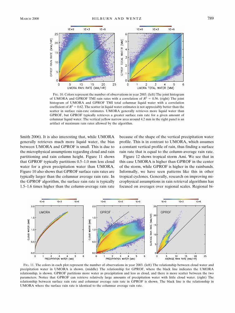
Smith 2006). It is also interesting that, while UMORAgenerally retrieves much more liquid water, the biasbetween UMORA and GPROF is small. This is due tothe microphysical assumptions regarding cloud and rainpartitioning and rain column height. Figure 11 showsthat GPROF typically partitions 0.5–1.0 mm less cloudwater for a given precipitation water than UMORA.Figure 10 also shows that GPROF surface rain rates aretypically larger than the columnar average rain rate. Inthe GPROF algorithm, the surface rain rate is typically1.5–1.6 times higher than the column-average rain rate

because of the shape of the vertical precipitation waterprofile. This is in contrast to UMORA, which assumesa constant vertical profile of rain, thus finding a surfacerain rate that is equal to the column-average rain rate.

Figure 12 shows tropical storm Ami. We see that inthis case UMORA is higher than GPROF in the centerof the storm, while GPROF is higher in the rainbands.Informally, we have seen patterns like this in othertropical cyclones. Generally, research on improving mi-crophysical assumptions in rain retrieval algorithms hasfocused on averages over regional scales. Regional bi-

FIG. 10. Colors represent the number of observations in year 2003. (left) The joint histogramof UMORA and GPROF TMI rain rates with a correlation of R2 � 0.56. (right) The jointhistogram of UMORA and GPROF TMI total columnar liquid water with a correlationcoefficient of R2 � 0.62. The scatter in liquid water estimates is not appreciably better than thescatter in surface rain-rate estimates. UMORA generally retrieves more liquid water thanGPROF, but GPROF typically retrieves a greater surface rain rate for a given amount ofcolumnar liquid water. The vertical yellow narrow area around 4.2 mm in the right panel is anartifact of maximum rain rates allowed by the algorithm.

FIG. 11. The colors in each plot represent the number of observations in year 2003. (left) The relationship between cloud water andprecipitation water in UMORA is shown. (middle) The relationship for GPROF, where the black line indicates the UMORArelationship, is shown. GPROF partitions more water as precipitation and less as cloud, and there is more scatter between the twoparameters. Notice that GPROF can retrieve relatively large amounts of precipitation water with little cloud water. (right) Therelationship between surface rain rate and columnar average rain rate in GPROF is shown. The black line is the relationship inUMORA where the surface rain rate is identical to the columnar average rain rate.


Fig 10 11 live 4/C

ases can occur because of differences in the relativeproportions of different types of precipitation. Differ-ent types of precipitation, however, are also often or-ganized, more fundamentally, on storm scales (e.g.,Parker and Johnson 2000). We believe that further un-derstanding and improvements will be made, not somuch in analyzing how assumptions affect average val-ues, but in analyzing how changes in assumptions affectstorm-scale structure.

To assess UMORA SSM/I rain rates, the first step isto assess the consistency among F08, F10, F11, F13, F14,and F15. This is obviously complicated by the fact thatthe SSM/I cover different time periods. Also, the SSM/Imeasure at different local times of day—introducingreal geophysical differences. To intercalibrate the rainrates from the different SSM/I sensors for our trendanalysis, we apply a scaling factor to rain rate. Thescaling factors were calculated by matching F13 to TMIin the tropics, and then working backward in timematching F15, F14, and F11 to F13 globally, F10 to F11globally, and F08 to F10 globally. The resulting scalingfactors are shown in the middle column of Table 3. Thisprocedure using overlap periods to remove intersatel-lite offsets is similar to that done when constructingclimate data records from other satellite sensors, suchas the Microwave Sounding Unit (Mears et al. 2003).The SSM/I scale factors confirm what our experiencewith the data has indicated: overall the SSM/I are ingood agreement, with the exception of F10, which hasknown sensor and satellite problems. The scaling fac-tors also confirm the general rule that late-morning sat-ellites (such as F14 and F15) tend to have rain rates thatare a little low, whereas early-morning satellites (suchas F08, F11, and F13) tend to have averages that are alittle high. These general rules are suggestive of diurnalbiasing.

To further investigate diurnal biasing, we used

FIG. 12. Tropical Storm Ami at 2000 UTC 12 Jan 2003: (top)UMORA rain rates, (middle) GPROF, and (bottom) theUMORA – GPROF difference (mm h�1). The data have beenput on a quarter-degree grid and only data over the ocean areshown. This shows how differences between UMORA andGPROF organize themselves on storm scales. UMORA is higherin the center of the tropical storm and GPROF is higher in thespiral bands.

TABLE 3. The scaling factors to achieve agreement amongSSM/I rain rates based on overlap periods. The scaling factorswere calculated by matching F13 to TMI in the tropics, and thenworking backward in time matching F15, F14, and F11 to F13globally; F10 to F11 globally; and F08 to F10 globally. The diurnalscaling factors were derived from the TMI diurnal cycle as shownin Fig. 12. This table shows that much of the discrepancy amongvarious SSM/Is is due to time-of-day effects, with the notableexception of F10, which has known instrument problems.

Satellite Scaling Diurnal scaling

F08 0.990 0.992F10 0.908 1.023F11 0.983 0.994F13 0.964 0.991F14 1.015 1.012F15 1.031 1.024


Fig 12 live 4/C

UMORA TMI to estimate the impact of the diurnalcycle on SSM/I rain measurements. The diurnal cycle inUMORA TMI rain rates (Fig. 13) match the well-known diurnal cycle of rain over the oceans with anearly-morning peak (Imaoka and Spencer 2000). Whilethe diurnal cycle has a strong first harmonic, the morn-ing peak and evening trough have different shapes thatproduce small biases. Using this diurnal cycle fromUMORA TMI and local equatorial crossing times fromSSM/I we find that, indeed, early-morning satellitestend to have averages that are a little high (and thusneed to be adjusted lower) and late-morning satelliteshave averages that are a little low (and need to beadjusted higher). Scaling coefficients based on just di-urnal effects are given in the rightmost column of Table3. We have also performed a much more detailed analy-sis using the actual times for each SSM/I pixel (ratherthan equatorial crossing times) and find similar behav-ior. We see that diurnal effects account for much of thedifference between various SSM/Is. Except for F10, the

residual intersatellite bias is less than 3%, which indi-cates the SSM/I TB have been well intercalibrated. Wemight have expected even smaller residual biases giventhat the over-ocean intercalibration is estimated to beat the 0.1-K level. However, the over-ocean calibrationis done for rain-free scenes for which very accurateradiative transfer models are available. The brightnesstemperatures for moderate to heavy rain can be 100 Kwarmer than these calibration scenes, and nonlinearityin the radiometer response function or multiplicativeerrors arising from small errors in spillover or hot loadspecification may be responsible for the small residualerrors. The F10 SSM/I remains somewhat of a mysteryto us, and the exact cause of its calibration problems isan open issue. Please note that none of the correctionfactors shown in Table 3 are applied to our publiclyavailable data. Once we better understand their physi-cal basis, we will account for them using a more rigor-ous process.

Having assessed the agreement among SSM/I, we ap-

FIG. 13. (top) Local equatorial crossing times of the ascending node for the Defense Me-teorological Satellites Program series of SSM/I. Note that F08 is 12 h out of phase with theother satellites, so the descending node time is plotted. (middle) The ratio of hourly rain to thedaily mean based on TMI for 1998–2005. While the cycle had a strong first harmonic, theearly-evening trough is slightly flatter than the early-morning peak, thus leading to smallsystematic biases. (bottom) The diurnal corrections implied by the SSM/I crossing times andthe TMI diurnal cycle are shown. Average values are given in the right column of Table 3.Note that in general, late-morning satellites (F10, F14, and F15) have adjustments that in-crease the average, whereas early-morning satellites (F08, F11, and F13) have adjustments thatdecrease the average.


Fig 13 live 4/C

ply the scale factors in Table 3 and compare UMORASSM/I with GPCP. Figure 14 shows that UMORASSM/I and GPCP agree well in the tropics, but theGPCP dataset has considerably more precipitation inthe extratropics. This extra precipitation causes GPCPto be about 20% higher the UMORA SSM/I in theglobal average. The source of this difference is unclear.It is possible that GPCP retrieves more precipitation inmidlatitudes because of its use of infrared satellite data.It is possible that UMORA retrieves less precipitationbecause it only considers liquid precipitation. Wentz etal. (2007) address this issue from a hydrological balanceperspective, and their results suggest that UMORArain rates may be too low in mid–high latitudes but thatthe truth cannot be too much higher than GPCP values.This would point to rain column heights that need to belower in midlatitudes (closer to the ITU values in Fig.6) or vertical rain profiles that have R/R(0) � 1 in mid-latitudes (meaning that the surface rain rate is higherthan the columnar rain rate). Figure 14 also compareslinear trends. Overall, these two datasets have remark-ably similar trends, both in spatial pattern and magni-tude. Both datasets have roughly a 10% increase inprecipitation in the ITCZ and over the western Pacificwarm pool. The GPCP has a much stronger increase inthe Indian Ocean than UMORA SSM/I. Annual aver-age time series are shown in Fig. 15. After 1997, thetime series are remarkably similar, both globally and inthe tropics. It is unclear why the datasets differ before1997. Figure 15 also compares SSM/I versus the SSM/I

“backbone,” which is calculated using just one SSM/I ata time. That is, the backbone starts with F08 and thenswitches to F10 when it is available, then to F11 when itis available, and finally to F13 when it is available. Thus,the changing number of SSM/I is not a large source ofuncertainty, and SSM/I backbone trend maps (notshown) are very similar to the SSM/I trend map in Fig.14. Figure 15 also shows that UMORA TMI agrees wellwith UMORA SSM/I and GPCP in the tropics. Theglobal average trends are �1.5%, �1.8%, and �2.4%decade�1 for GPCP, UMORA SSM/I, and theUMORA SSM/I backbone, respectively. The tropicaltrends are �2.7%, �2.0%, and �3.5% decade�1 forGPCP, UMORA SSM/I, and the UMORA SSM/Ibackbone, respectively. The differences between thesetrends indicate the sensitive nature of trend analysis.

5. Conclusions

The Unified Microwave Ocean Retrieval Algorithm(UMORA) provides a consistent 18-yr record of simul-taneous retrievals of sea surface temperature, windspeed, water vapor, cloud water, and rain rate fromSSM/I, TMI, and AMSR-E. Brightness temperatureshave been intercalibrated to the 0.1-K level. The raincomponent of UMORA is an improvement of theWS98 rain algorithm. Several problems with the WS98algorithm were found (resampling, beamfilling, andrain column height) and were corrected in a physicallyconsistent manner. In particular, the rain column height

FIG. 14. (top left) The 1988–2005 GPCP mean rain rate and (bottom left) UMORA rain rate from all SSM/I (mm day�1). GPCP hasan area-weighted average of 2.99 mm day�1 over the ocean during this time period. UMORA has an area-weighted average of 2.46 mmday�1. (top right) The 1988–2005 GPCP linear trend in rain rate and (bottom right) the UMORA rain-rate trend from all SSM/I (mmday�1 decade�1). The global average trends are �1.5% and �1.8% decade�1 for GPCP and UMORA SSM/I.


Fig 14 live 4/C

is more realistic and a beamfilling correction is appliedthat agrees with simulation results. The UMORAbeamfilling correction explicitly accounts for radiom-eter saturation and footprint-resolution effects. Oncethese corrections are applied, the UMORA rain re-trievals are consistent across satellite platform and sen-sor type. It is shown that much of the small remainingdifferences among UMORA SSM/I rain retrievals aredue to real geophysical time-of-day effects. When diur-nal effects are removed, the agreement among theSSM/I, TMI, and AMSR-E rain rates are within �3%,except for SSM/I F10, which has a unique set of cali-bration problems. The remaining discrepancy may bedue to nonlinearity in the calibration equation or mul-tiplicative errors arising from small errors in spilloveror hot load specification.

UMORA rain retrievals are in reasonable agreementwith other datasets. UMORA TMI retrievals agreevery well on average with GPROF TMI retrievals.However, a comparison of instantaneous pixel-to-pixelretrievals showed large differences that are due to dif-ferent microphysical assumptions. UMORA SSM/Iagree well with GPCP in the tropics, however GPCPhas greater precipitation in the extratropics. Trends inall of the datasets have similar spatial patterns andagree to within 50% on average. Despite the remaining

uncertainties in passive microwave rain retrieval, theoverall similarity of trends in the datasets suggests thatthe rain rates can be used with reasonable confidencefor climate studies on time scales of years to decades.

Acknowledgments. We are very grateful for continu-ing support from the National Aeronautics and SpaceAdministration (NASA). We are thankful to the De-fense Meteorological Satellite Program for making theSSM/I data available to the civilian community. Wehave been supported by NASA NEWS under ContractNNG05OAR4311111 and by DISCOVER, which issupported by the NASA Earth Science Research, Edu-cation, and Applications Solution Network (REASoN)Project under Cooperative Agreement NNG04GG46A.REASoN is a distributed network of data and informa-tion providers for NASA’s Earth Science Enterprise(ESE) Science, Applications, and Education programs.REASoN provides vital links between NASA’s data,modeling, and systems engineering capabilities and theuser communities in research, applications, and educa-tion. The AMSR-E work was partially supported byNASA Contract NNG04HZ47C. We are grateful tothree anonymous reviewers whose comments havegreatly enhanced the clarity of this paper.

The GPCP combined precipitation data were devel-

FIG. 15. Time series of annual rain-rate anomalies from the 18-yr (1988–2005) average for GPCP(black dot, solid line), UMORA SSM/I (red dot, solid line), and UMORA SSM/I using just the “back-bone” of SSM/I (red x, dashed line) for (top) the global ocean and (bottom) the tropical ocean from 20°Nto 20°S. The bottom panel also shows UMORA TMI (blue asterisk, solid line). The SSM/I backbone usesjust one SSM/I at a time, starting with F08, then switching to F10 when it becomes available, then to F11when it becomes available, and finally to F13 when it becomes available. The backbone shows that thechanging number of SSM/I in the average of all SSM/I is not a significant source of uncertainty in globalaverage time series. Notice that GPCP is well correlated with UMORA after 1997, but the correlationbetween the time series is lower prior to 1997.


Fig 15 live 4/C

oped and computed by the NASA Goddard SpaceFlight Center’s Laboratory for Atmospheres as a con-tribution to the GEWEX Global Precipitation Clima-tology Project. GPROF TMI data used in this studywere acquired as part of the Tropical Rainfall Measur-ing Mission (TRMM). The algorithms were developedby the TRMM Science Team. The data were processedby the TRMM Science Data and Information System(TSDIS) and the TRMM Office; they are archived anddistributed by the Goddard Distributed Active ArchiveCenter. TRMM is an international project jointly spon-sored by the Japan National Space DevelopmentAgency (NASDA) and the U.S. NASA Office of EarthSciences.

REFERENCES

Adler, R. F., and Coauthors, 2003: The version 2 Global Precipi-tation Climatology Project (GPCP) Monthly PrecipitationAnalysis (1979–present). J. Hydrometeor., 4, 1147–1167.

Ashcroft, P., and F. J. Wentz, 2000: Algorithm theoretical basisdocument: AMSR level 2A algorithm. RSS Tech. Rep.121599B-1, Remote Sensing Systems, 29 pp.

Fiorino, S. T., and E. A. Smith, 2006: Critical assessment of mi-crophysical assumptions within TRMM radiometer rain pro-file algorithm using satellite, aircraft, and surface datasetsfrom KWAJEX. J. Appl. Meteor. Climatol., 45, 754–786.

Hilburn, K. A., F. J. Wentz, D. K. Smith, and P. D. Ashcroft, 2006:Correcting active scatterometer data for the effects of rainusing passive radiometer data. J. Appl. Meteor. Climatol., 45,382–398.

Hogg, R. A., and E. A. Tanis, 1997: Probability and StatisticalInference. 5th ed. Prentice Hall, 722 pp.

Imaoka, K., and R. W. Spencer, 2000: Diurnal variation of pre-cipitation over the tropical oceans observed by TRMM/TMIcombined with SSM/I. J. Climate, 13, 4149–4158.

International Telecommunication Union, 1999: Specific attenua-tion model for rain for use in prediction methods. ITU-RRecommendation P.838, 2 pp.

——, 2001: Rain height model for prediction methods. ITU-RRecommendation P.839, 2 pp.

Kummerow, C., and Coauthors, 2001: The evolution of the God-dard Profiling Algorithm (GPROF) for rainfall estimationfrom passive microwave sensors. J. Appl. Meteor., 40, 1801–1820.

Liu, G., and Y. Fu, 2001: The characteristics of tropical precipi-

tation profiles as inferred from satellite radar measurements.J. Meteor. Soc. Japan, 79, 131–143.

Mears, C. A., M. C. Schabel, and F. J. Wentz, 2003: A reanalysisof the MSU channel 2 tropospheric temperature record. J.Climate, 16, 3650–3664.

Meissner, T., and F. J. Wentz, 2002: An updated analysis of theocean surface wind direction signal in passive microwavebrightness temperatures. IEEE Trans. Geosci. Remote Sens.,40, 1230–1240.

——, and ——, 2004: The complex dielectric constant of pure andsea water from microwave satellite observations. IEEETrans. Geosci. Remote Sens., 42, 1836–1849.

Parker, M. D., and R. H. Johnson, 2000: Organizational modes ofmidlatitude mesoscale convective systems. Mon. Wea. Rev.,128, 3413–3436.

Petty, G. W., 1994: Physical retrievals of over-ocean rain rate frommultichannel microwave imagery. Part I: Theoretical charac-teristics of normalized polarization and scattering indices.Meteor. Atmos. Phys., 54, 79–99.

——, 1995: Frequencies and characteristics of global oceanic pre-cipitation from shipboard present-weather reports. Bull.Amer. Meteor. Soc., 76, 1593–1616.

Poe, G. A., 1990: Optimal interpolation of imaging microwaveradiometer data. IEEE Trans. Geosci. Remote Sens., 28, 800–810.

Reynolds, R. W., N. A. Rayner, T. M. Smith, D. C. Stokes, and W.Wang, 2002: An improved in situ and satellite SST analysisfor climate. J. Climate, 15, 1609–1625.

Spencer, R. W., H. M. Goodman, and R. E. Hood, 1989: Precipi-tation retrieval over land and ocean with the SSM/I: Identi-fication and characteristics of the scattering signal. J. Atmos.Oceanic Technol., 6, 254–273.

Stogryn, A., 1978: Estimates of brightness temperatures fromscanning radiometer data. IEEE Trans. Antennas Propag.,26, 720–726.

Varma, A. K., G. Liu, and Y.-J. Noh, 2004: Subpixel-scale vari-ability of rainfall and its application to mitigate the beam-filling problem. J. Geophys. Res., 109, D18210, doi:10.1029/2004JD004968.

Wentz, F. J., 1997: A well-calibrated ocean algorithm for specialsensor microwave/imager. J. Geophys. Res., 102, 8703–8718.

——, and R. W. Spencer, 1998: SSM/I rain retrievals within aunified all-weather algorithm. J. Atmos. Sci., 55, 1613–1627.

——, and T. Meissner, 2000: AMSR ocean algorithm, version 2.RSS Tech. Rep. 121599A-1, Remote Sensing Systems, 66 pp.

——, P. D. Ashcroft, and C. L. Gentemann, 2001: Post-launchcalibration of the TRMM microwave radiometer. IEEETrans. Geosci. Remote Sens., 39, 415–422.

——, L. Ricciardulli, K. Hilburn, and C. Mears, 2007: How muchmore rain will global warming bring? Science, 317, 233–235.


intercalibrated passive microwave rain products from the

Documents