Interactive Teachers’ Resource on the Acoustics of Pipes

Viktor Cragéus

Supervisor: Sten Ternström

Examiner: Sten Ternström

Examensarbete i Musikakustik

(Master Thesis in Music Acoustics)

KTH - School of Computer Science and Communication (CSC) Department of Speech, Music and Hearing

S-100 44 Stockholm Stockholm

23 February 2007

Abstract Today, conventional textbook education is not seen as a very effective teaching method. A less static form of education is considered more useful [15], [24]. “Learning by doing” or by experimenting is such a form. Students today are well acquainted with computers. This is why the demand is rising for replacing classic experiments with computer based setups. Developments of physical modeling synthesis have seen substantial improvements during the latest years. The use of simulations to demonstrate physics is cheap and effective but suffers from the risk of losing connection with reality. An experiment on the acoustics of pipes is presented which combines interactive computer measurement software with a physical pipe. The materials needed to conduct the experiment are hosted on a newly developed web portal, complete with manuals and software. The experiment is evaluated in terms of accuracy and usability. Feedback from teachers indicates that the experiment is ready for use in education of high school students.

Keywords: acoustic, experiment, music, sound, teachers resource, pipes.

Sammanfattning Interaktiv webbresurs om pipors akustik för Fysik B

Ren textboksundervisning ses idag som en mindre effektiv undervisnings-form. En mindre statisk undervisning ses som mer användbar [15], [24]. Inlärning genom att undersöka eller att experimentera är en av dessa former. Studenter idag är vana att använda datorer. Därmed öppnar sig möjligheten att byta ut klassiska experiment mot datorbaserade sådana. Utvecklingen av fysisk simulering har dramatiskt förbättrats de senaste åren. Att demonstrera fysik med hjälp av simuleringar är billigt och effektivt, men problemet uppstår lätt att man förlorar känslan för verkligheten. Ett experiment baserat på akustik i pipor presenteras som kombinerar mjukvara för mätningar med en fysisk pipa. Materialet som behövs för att utföra experimentet presenteras på en utvecklad webb-portal, komplett med manualer och mjukvara. Experimentet utvärderas med avseende på exakthet och användbarhet. Synpunkter inhämtade från lärare tyder på att experimentet är färdigt att användas för undervisning av gymnasieelever.

Nyckelord: akustik, experiment, ljud, musik, lärarresurs, pipor.

Acknowledgments I specially would like to thank my supervisor Sten Ternström, RealSimPLE team member Kahl Hellmer and the other members of the RealSimPLE project team. Your feedback has been invaluable for me during this project. I would also like to thank the teachers at Kärrtorps Gymnasium (high school) for providing their thoughts about how to make a useful and interesting experiment. I would also direct thanks to all of the people asking and answering questions on the PD mailing list Archives, they have been very helpful.

List of Figures

Figure 1: Schematic visualization of sound, from source to receiver.................... 3 Figure 2: Two periods of a 100 Hz sine wave (left) and two periods of a sound wave produced by a wooden flute sample (right)................................................... 4 Figure 3: Spectrum of a 100 Hz sine wave (left) and the spectrum of a wooden flute sample (right).................................................................................................. 5 Figure 4: FFT waterfall plot of a wooden flute sound sample............................... 6 Figure 5: Picture of a Helmholtz resonator............................................................ 8 Figure 6: A version of the Kundt´s tube experiment. ............................................ 8 Figure 7: Drawing of a reed (left) and a clarinet as an example of a reed instrument (right). ................................................................................................. 10 Figure 8: Sketch of a flute mechanism (left) and a recorder as an example of flutes (right). ......................................................................................................... 10 Figure 9: Generic sketch of brass instrument (left) and a trumpet as an example of a brass instrument (right).................................................................................. 11 Figure 10: Basic illustration of the SimPLEK´s Tube Experiment setup. ........... 14 Figure 11: PVC plastic tubing used in the experiment ........................................ 15 Figure 12: Attachment material options for the PVC plastic tubing, connector (left) and electrical tape (right) ............................................................................. 15 Figure 13: The miniature loudspeaker used in this project.................................. 16 Figure 14: Miniature microphone used in this project......................................... 16 Figure 15: Flowchart of the measurement/visualization software architecture... 17 Figure 16: The main PD patch for the measurement software ............................ 17 Figure 17: Screenshot of the measurement/visualization software. .................... 18 Figure 18: Additive flute synthesis software architecture featured ..................... 20 Figure 19: ADSR amplitude envelopes in the additive flute synthesis. .............. 20 Figure 20: Screenshot of the start page from the website created for the Swedish part of the RealSimPLE project. ........................................................................... 23 Figure 21: Frequency response of the experiment setup ..................................... 25 Figure 22: PVC tube extension piece alternatives ............................................... 30 Figure 23: Impulse response of the experiment setup.. ....................................... 32

List of Symbols

dB decibel F force f frequency Hz Hertz L length P pressure vs sound velocity T time period λ wavelength

List of Abbreviations

ADSR Attack Decay Sustain Release CSS Cascading Style Sheets H.O.T Higher Order Terms FFT Fast Fourier Transform FT Fourier Transform OS Operating System PD Pure Data

Contents Abstract Sammanfattning Acknowledgments List of Figures List of Symbols List of Abbreviations Preface.................................................................................................................... 1 1 The Concept of Sound ....................................................................................... 3

1.1 Physics of a Sound Wave.............................................................................. 3 1.2 Properties of Sound....................................................................................... 4 1.3 Musical Aspects of Sound ............................................................................ 6

2 Acoustics in Pipes ............................................................................................... 7

2.1 The Phenomenon of Resonance.................................................................... 7 2.2 Wave Propagation in a Cylinder ................................................................... 8 2.3 Control Mechanisms of Acoustic Length ..................................................... 9 2.4 Instruments with a Cylinder-like Bore........................................................ 10

3 Pedagogical Viewpoints ................................................................................... 11

3.1 Principles of Learning................................................................................. 11 3.2 Adaptation of the Complexity Level........................................................... 12 3.3 Creation of a Stimulating Experiment ........................................................ 13

4 The SimPLEK´s Tube Experiment.................................................................. 14

4.1 Bore model.................................................................................................. 15 4.2 Source of Excitation.................................................................................... 15 4.3 Sensor choice .............................................................................................. 16 4.4 Measurement and Visualization Software .................................................. 16 4.4 Applications of the SimPLEK´s Tube ........................................................ 20

5 Web Portal ........................................................................................................ 21 6 Experiment Evaluations .................................................................................. 23

6.1 Model Performance..................................................................................... 23 6.2 Focus group results ..................................................................................... 25

7 Discussion and Conclusions ............................................................................ 26 8 Future Work..................................................................................................... 30

8.1 Minor Improvements .................................................................................. 30 8.2 College Level Extension ............................................................................. 31

References ............................................................................................................ 33 A Questionnaire .................................................................................................. 36 B SimPLEK´s Tube Construction Manual 37 C SimPLEK´s Tube Operating Manual 45 D SimPLEK´s Tube Lab Manual 51

Preface

From ancient times to the modern day, music has played an important role in people’s everyday lives. Music offers an alternate route for expressing and/or sensing emotions. It is often used for enhancing emotions, like for example Samuel Barber’s Adagio for Strings op. 11 which is often played in combination with some dramatic or sad episode of a movie. Another example one could think of is a party without music. In many peoples’ opinion, this would mean a state of mind very far from “euphoria”. We even have musical terms like Con amore (with love) and Misterioso (mysterious) for describing its mood. To capture the core of musical acoustics in a single sentence, one can quote Fletcher and Rossing [14] “Our understanding of a particular area will be reasonably complete only when we know the physical causes of the difference between a fine instrument and one judged to be of mediocre quality”. Throughout history, instrument manufacturers have based their craftsmanship on empirical trial and error methods. Scientific analyses of music and instruments, which date back to the last two centuries, are young compared to how long instruments and music have been around us. For instance, the oldest flute discovered dates back some 35 000 years [4]. Experiments are an effective form of teaching, especially when applying cognitive methods for problem solving. This was for example shown by research on students in China performed by Gang [15]. The research also points out the danger of using experiments which are too abstract for the students to comprehend. Hence is it important when performing experiments to stimulate the cognitive thought process of the students. Hunt [18] recently observed that the rate of drop-outs and failures is increasing in physics courses. One way of overcoming this problem is to use experiments that are meaningful to the students; that they can relate to their life experience. Hunt also demonstrated that it is possible to devise quantitative experiments in elementary physics without the need for special laboratory equipment. Recent advances in mathematical tools and computer technology has made it possible to make fairly realistic equations/models of almost every acoustic instrument. In particular, research performed by Benade [3], Coltman [10], Helmholtz [9], Hirschberg [19], Keefe [20], Smith [39], Välimäkki [41] and others, has been important for the modelling of the physics in our tube-like instruments. We can hear many of these physical models implemented in a modern synthesizer which digitally tries to emulate real acoustic instruments. This makes it interesting to start comparing the performance of synthesis against real acoustic instruments.

1

Since many people have a close relationship to music either as listeners or as practising musicians, the theory behind music should be an excellent starting point to motivate further studies in the area of acoustics. Knowledge about acoustics involves several basic concepts such as differential equations, waves and Newtonian physics, which are key to understanding other areas of physics. Therefore, an increased interest in acoustical theory could serve a second purpose as an inroad to the whole science of physics. This thesis is part of the RealSimPLE project, which is collaboration between the TMH department at KTH and the CCRMA at Stanford University. The goal is to provide teachers at high school and college level with a set of inspiring experiments based on acoustics, where hands-on models of reality are combined with computer simulations. This specific part of the project concerns the acoustics of pipes. The primary goal for this thesis was to produce a low cost, easily built and interesting experiment that demonstrates several acoustic properties of pipes. The setup consists of four main parts: a real world pipe object, a microphone sensor for collecting measurement data, an excitation system for generation of air pressure, and computer software built with the freely distributable Pure Data1 framework for measurements/visualisations. The actual simulation part of the experiment will be implemented at Stanford University and is not included in this thesis. For more information on the project the reader is referred to the full documentation of the RealSimPLE project [21] and the RealSimPLE project website [31]. Chapter 1 begins with a brief overview of sound, both from a scientist’s as well as a musician’s perspective. Special attention is directed towards the conversion from pressure to audible sound in our ears. Chapter 2 addresses the basics of acoustics in pipes. The chapter also presents an introduction to the acoustics of various cylinder-like instruments. Chapter 3 presents some brief advice on how to make an experiment interesting. Chapter 4 specifies the SimPLEK´s Tube experiment, developed in this project. Chapter 5 describes the development of the RealSimPLE project web portal at KTH. Chapter 6 contains the evaluation of the experiment with respect to several criteria. Chapter 7 presents the conclusions and discusses the experiment developed during this master thesis. Chapter 8 suggests possible future developments for this specific part of the RealSimPLE project. 1 “PD (aka Pure Data) is a real-time graphical programming environment for audio, video, and graphical processing. It is the third major branch of the family of patcher programming languages known as Max (Max/FTS, ISPW Max, Max/MSP, jMax, etc.) originally developed by Miller Puckette and company at IRCAM” [21].

2

1 The Concept of Sound

1.1 Physics of a Sound Wave Sound is basically local pressure variations in any medium, where the most common medium is air. One way to think of sound [26] is to imagine slicing up a volume of air into several small local segments. The instant when the first of these local segments senses an incoming pressure wave, it becomes compressed and wants to expand in the direction of the following segment. The next segment then in turn senses a force and responds similar to the first segment. But when a segment expands, the pressure within that that segment will lower, which creates a retracting force. The end result will be that each segment of air will oscillate back and forth from its original position creating a traveling pressure/sound wave.

Figure 1: Schematic visualization of sound, from source to receiver. The speed of a sound wave traveling in air is determined by the following relation [35]:

Expression (1) evaluated for normal values of air pressure and room temperature gives a value of the speed of sound in air of vs ≈ 344m/s. (Coefficients cp and cv denotes the specific heats at constant pressure and constant volume respectively and ρ corresponds to density). Oscilloscope analysis of sound reveals that its waveform often resembles the shape of a sinusoidal wave. One way to explain why sounds display the shapes of sine waves is by going backwards and start looking at the detection unit. That is investigating what happens when pressure variations reach our ears [4] or alternatively a microphone. In reality the last outpost before the brain detects a sound is the fine hair cells in the basilar membrane. For a more detailed description of the function human ear see [29]. Now suppose that y denotes the distance of the eardrum from its equilibrium. Its elastic property gives that a restoring force F will enter as soon as a pressure variation in the air moves the eardrum from its equilibrium. Let this force be some constant times the

p

sv

c Pvc ρ

=

(1)

3

distance y. The resulting equation combined with Newton´s second law of motion will then be:

The solution to this equation is well known and can be written on the following general form:

0kyym

+ =&&

(2)

cos sink ky A B

mt mt= + (3)

This is a somewhat simplified version of reality, but it clearly demonstrates that the vibrations of the eardrum can be described by equations of a sine character. These equations can be used in a similar fashion for analyzing the way the hair cells in the basilar membrane respond to pressure variations.

1.2 Properties of Sound For describing different types of sound there is a set of defined basic properties. Frequency is a measure of how often something is happening. In the case of sound, frequency is how many times per second the sound wave repeats itself. A good example is had by pulling a comb along a sharp edge [2]. This produces a snap each time a pin of the comb hits the edge. If pulled slowly, every snap is heard, but if the speed is increased, the individual snaps will blur together into a single tone. This results from the time resolution of a human ear being lower than the time interval between the snaps from the comb.

1fT

= (4)

Figure 2: Two periods of a 100 Hz sine wave (left) and two periods of a sound wave produced by a wooden flute sample from IK Multimedia Sampletank© (right).

4

Sounds of the same frequency do not sound the same because most sound has energy at several frequencies. A tuning fork only produces a single frequency when it is struck, while white noise has energy at all frequencies. Still musical sound waves display a nominal periodicity [4] and expression (4) can then be applied to derive a fundamental frequency. One way to extract the separate frequency components of a sound consisting of multiple frequencies is to compute the Fourier transform (FT). The FT brings out the energy in each of the present frequencies of the sound. In essence, the FT decomposes or separates a waveform or function into sinusoids of different frequency which sum to the original waveform (for examples see figure 3 and 4). This implies that it is possible to build a complex but stationary sound by adding a number of sine waves, each with its own amplitude, frequency, and phase parameters. In general, waveforms with time-domain discontinuities require an infinite number of sinusoids to be perfectly reconstructed. Figure 3: Spectrum of a 100 Hz sine wave (left) and the spectrum of a wooden flute sample from IK Multimedia Sampletank© (right). In reality the properties of sounds are even more complex. General “everyday” sounds we hear include a portion of noise or non-periodic sound. Also the amplitudes of the harmonics vary over time. The increased complexity is partly a result from factors such as that the acoustic impedance damps various frequencies differently. This is visualized in figure 4 on the following page, where the spectrum of a flute sample is plotted over time.

5

Figure 4: FFT waterfall plot of a Tom drum sample from Native Instruments Battery library©. Plot made with methods as suggested by Zölzer [42].

Sound pressure level [37] is a scaled version of pressure, based on our threshold of hearing. The scaling is done for practical reasons, since the range spanned by the previous mentioned threshold is quite large (0.00002 – 20 Pa).

20

20 log ( )nPLP

= dB

(5)

Where L0 = 0.00002 is the reference pressure. Zero dB will then represent an inaudible sound, whereas 120 dB will be a painfully loud sound, like standing close to a jet plane engine.

1.3 Musical Aspects of Sound Musicians describing a particular sound will most likely use terms like timbre, loudness, pitch, dynamics and duration. The timbre of a specific sound corresponds acoustically to the number of harmonics and the amplitude of each harmonics. A bright timbre would then mean that the sound has strong harmonics at high frequencies. Pitch and frequency are somewhat alike but are not to be mistaken for each other. The current practice in western music is based on our perception of evenly spaced sound [2], [26]. Pitch is hence related to our perception of sound whereas frequency is the physical measure of how many vibrations occur in one second. The A note above middle C on a Piano (A4) is determined to be of concert pitch with fundamental frequency 440 Hz. The next A note in succession (A5) has the fundamental frequency 880 Hz and so on. The same principle goes for the A note below middle C (A3) which is standardized to 220 Hz. If you play all notes (both black and white one) between for example middle A and the next A. Then you have played in total twelve tones named semitones or all together a whole octave. To further divide pitch into fractions, cents are used which are hundredths of a semitone. Two and three times the fundamental frequency and so on are often referred to as the second and the third partial tone or alternatively as the first and second

6

overtone. The former expression is preferred by acousticians, because the number of the partial is also the multiplier for the partial tone frequency, relative to the fundamental frequency. Dynamics is a term is related to volume or loudness. If you read a musical score, you will find markings like p for piano (Italian for quiet), pp for pianissimo (very quiet), f for forte (loud) and ff for fortissimo (very loud) [28]. These tell the player how hard the keys are supposed to be struck or the flute to be blown. The amount of energy used when exciting an instrument is directly related to the amplitude of the generated sound and therefore also directly related to its loudness. The term duration refers to how long a tone sounds, which is closely related to the amplitude and the transient behavior. A more detailed explanation [32] would be to divide the duration into four phases: Attack, Decay, Sustain and Release; often denoted as ADSR. Attack is how much time elapses from a key is pressed on an instrument till the sound reaches peak amplitude. The time to lower from peak amplitude to steady state is denoted decay. Finally, the release parameter is how long it takes for the sound to reach zero amplitude measured from the time when it is keyed off. ADSR is a convenient simplification of many common amplitude envelopes.

2 Acoustics in Pipes

2.1 The Phenomenon of Resonance The frequency or frequencies at which an object tends to vibrate with when hit, struck or somehow disturbed is known as the natural frequency of the object. Resonance occurs when an applied force near an object’s natural frequency results in a dramatic increase in amplitude of the object’s vibrations. The reason for this is that the applied force is in phase with the velocity and hence the transferred power from the applied force is maximized [35]. An easy way to think of resonance is to imagine a playground swing [26], which gains in altitude, if pushed at the right instant of time. Performed with reasonable temporal accuracy, such pushes will increase the amplitude of the swinging motion through the added external force. If pushed at a less ideal time, the result will be a decaying amplitude. The same basic idea of resonance applies to virtually every musical instrument. A classic experiment on resonance is the Helmholtz resonator developed by the acoustical physics pioneer Helmholtz [9]. The experiment is based around a pressure cavity, in shape of a bottle. If the air in the pressure cavity (see figure 5) is compressed, then the air will start flowing out from the bottle since the pressure is higher within the cavity than outside [26]. This process will continue until the pressure inside the bottle is below atmospheric. This makes the pressure higher outside than inside the bottle and air will start to flow inside the bottle again. Now the system is back in its original state with high pressure inside the cavity and the process will start all over. However the process

7

will weaken over time and finally come to a state of rest due to energy losses. This is known as the decay of a resonance.

Figure 5: A Helmholtz resonator. A. Kundt was another active pioneer within the areas of sound and light. He developed a valuable method for the investigation of resonances in pipes, known as Kundt´s tube. The experiment is based on the fact that a fine powder, lycopodium, when spread inside a tube in which is established a vibrating column of air, tends to collect in heaps at the nodes. The distance between the heaps can then be measured [12].

Figure 6: A version of the Kundt´s tube experiment, originally developed by A. Kundt (image from www.physics.ucla.edu).

2.2 Wave Propagation in a Cylinder Not many instruments resemble the Helmholtz bottle discussed in the previous chapter. Rather, most wind instruments have a pipe along which the sound waves travel [26]. A sound wave traveling inside a cylinder open at both ends will be partially reflected each time it encounters a change in impedance. This will occur at both the openings. Since the air easily can flow out from the cylinder there is no way to put up a net pressure and each reflected wave will have unaltered air motion but opposite sign of pressure. This means that after the wave has traveled two times the length of the tube it is back in its original state. Then the process continues to repeat itself until energy losses drive it to a state of rest. When two similar waves meet traveling in opposite directions they form what is referred to as a standing wave. The name comes from the fact that the effect of the summation of two traveling waves with opposite directions, makes the net wave appear like it is standing still. Also, there is no net transportation of energy in these conditions. For a more complete picture of how a sound wave behaves inside a cylinder, it is necessary to take into account how the wave interacts with the walls inside the cylinder. The actual motion of the wave can then be separated into axial motion, transverse radial motion and transverse concentric motion. The resulting equation that describes the wave

8

inside the cylinder of infinite length and with H.O.T (higher order terms) disregarded becomes [14]:

2 2 2

2 2 2 2 2

1 1 1( )p p prr r r r x c tφ

∂ ∂ ∂ ∂ ∂+ + =∂ ∂ ∂ ∂ ∂

p (6)

2.3 Control Mechanisms of Acoustic Length The length of the cylinder is the main factor determining the resonant pattern of the cavity. Depending on whether the cylinder is open in both ends, closed in both or semi open, the patterns are defined by the following formulas [35]:

Open-Closed tube: ,....)7,5,3,1(4

×⋅

=L

vf sound (7)

Closed-Closed tube: .....)7,6,5,4,3,2,1(2

×⋅

=L

vf sound (8)

Open-Open tube: .....)7,6,5,4,3,2,1(2

×⋅

=L

vf sound (9)

During experiments it has been discovered that the actual physical length differs from the acoustical (efficient) length. The efficient length is given by the following end correction formula where r is the radius of the cylinder [13]:

A tone hole is an opening located on the bore of a wind instrument which, when covered, changes the pitch of the sound produced. For a pipe with no tone holes, the effective length is the acoustical length i.e. physical length plus end corrections. A shorter pipe, in other words, produces higher notes. An open hole in the side of the pipe shortens the pipe’s effective length and therefore raises the frequencies of the notes it produces. Generally a large hole in a given position decreases the effective length to something slightly larger than the effective length of a pipe cut off at that position and a smaller hole

Open-Closed effective tube length: 0.6effL L= + r (10)

9

produces a somewhat longer effective length. Covering the hole with a finger, or with a pad operated by a key, increases the effective length and lowers the pitch. If there are several tone holes, the first open tone hole usually has the largest influence on the pipe’s effective length. However, closing holes below the first open hole can lower the pitch significantly. Generally the pitch and timbre of the notes produced will depend on the positions, sizes, heights, and shapes of all the tone holes, both open and closed.

The implementation of register holes [26] is a way of letting the performer inhibit the buildup of a standing wave or specific resonance of the cavity, without much affecting other resonant patterns in the instrument. A register hole is a small hole strategically placed along the bore of the instrument. It is positioned where a certain standing wave pattern has a node and others have antinodes. This implies that by opening the hole which lets the air leak out, the pressure of that certain frequency is reduced which in turn decreases its amplitude while the standing waves of other resonances are left unaffected.

2.4 Instruments with a Cylinder-like Bore The one thing that many wind-instruments have in common is the feature of a resonant cavity shaped somewhat as a cylinder. Some instruments have bent cylinders and Bessel or bell shaped end sections. The main difference in the construction of wind-instruments is the way the resonance is driven [26]. Therefore the common practice is to divide these instruments into three main categories, based on the construction of the excitation device. Reed instruments drive their resonance [26] by a mechanical device called a reed. The reed is a thin and stiff piece of material which bends due to added pressure. It is mounted so that a small gap into the cavity is left open when no external pressure is added. Depending if the pressure is high or low behind the reed the gap opens or closes.

Figure 7: Drawing of a reed (left) and a clarinet as an example of a reed instrument (right), (image of clarinet from www.musikborsen.se). Flutes and Whistles are driven by air flow rather than pressure [26]. The air is blown into a tube section. This section is followed by a hole (duct/window) drilled at the top of the instrument. When the air reaches the far edge (labium) of that hole it gets divided into two separate flows. One stream of air flows into the resonant chamber and one stream flows out from the instrument.

Figure 8: Sketch of a flute mechanism (left) and a recorder as an example of flutes (right), (image of recorder from www.musikborsen.se).

10

Brass is the third main category of wind-instruments. The principle behind driving the resonance in brass instruments is that the player’s lips acts as a reed [26]. When the player tightens or loosens the lip-tension, the resonance frequency of the lips themselves varies. The resonance peaks of brass instruments are not completely regularly spaced in frequency. When the harmonic spectrum of the lip vibration matches a large number of impedance peaks in the instrument’s set of resonances, sustained vibration becomes possible. For any given fingering (tube length), the player can select one out of several tones by changing the lip tension only. That is why a trumpet needs only three valves.

Figure 9: Generic sketch of brass instrument (left) and a trumpet as an example of a brass instrument (right), (image of trumpet from www.musikborsen.se).

3 Pedagogical Viewpoints

3.1 Principles of Learning When creating an interesting experiment a good approach is to start looking at the basic principles that govern the human learning process. Following is a brief review of the different psychological principles involved in the learning process as presented in [29]. Tolman stated after many years of psychological experiments that “Learning is based on knowledge and expectation of “what leads to what”” According to Bandura the process of learning is done in four stages: Attention, retention, reproduction, motivation. To be able to learn you first need to focus. Then you need to be able to grasp what is being presented. In the next phase you have to possess the physical ability to reproduce the new skills or the intellectual ability to process the new information. Then finally for all this to take place you need to be motivated for doing it. Cognition psychology defines the moment of learning as the time when a new experience contradicts earlier expectations/experiences. This conflict has to be resolved and the involved thought process that processes the new information is what leads to new knowledge. Information is much more likely to be consolidated into our memory when there are several types of sensory stimuli available as for example sight, sound and sensation. Repetition is also an effective way for remembering things. Long time motivation for learning is likelier to be higher in an intrinsic form rather than extrinsic. In other words motivation is higher if the activity is performed for its own sake compared to if it is performed for receiving an external reward or avoiding a punishment.

11

People are more inclined to learn from a person that are like a role model or one whom they admire or consider to be more successful than others. It has also been concluded during experiments that it is much easier to learn something new when the information/skill is found useful. The conclusion from this is that learning depends on the personality of the tutor but it is also easier to be interesting if you have something interesting to mediate. The most basic reflex that all animals including humans posses innately is the orientation reflex. This reflex is a vital survival instinct that makes us react to sudden changes in our environment. This is because a sudden noise or light flash is likely to implicate danger. But to react on all such stimuli will be tedious and unpractical, so in reality if the same stimuli reappear many times the receptors in our brains reach a state of fatigue and we gradually stop paying attention to it. Attention will therefore in substantially larger degree be directed towards stimuli of shifting rather than static form. The goal of the whole process of learning is to reach insight i.e. the sudden perception of a useful relationship that helps to solve a problem. In the area of education this can be interpreted as when a student finds a solution to a problem.

3.2 Adaptation of the Complexity Level Constructing a useful experiment requires that the experiment be adapted towards the respective course requirements. It is also important to make a distinct differentiation between high school and college which have completely different course plans. The physics course in Swedish gymnasium (upper secondary school) that deals with the subject of sound and acoustics is the 150 points Fysik B course, which is taken in third grade (course plan specified by [36]). Some schools have made small alterations to the general course plan, referred to as a local course plan, which can contain additional subjects. In the USA, physics is included in the three year 6 credit science high school class (for more information see [9]). Swedish gymnasium course literature includes titles such as Quanta B [11] and Heureka! Fysik för Gymnasiskolans Kurs B [6]. One of the books used in the USA is Let´s Review Physics [23]. The subjects which all upper secondary school course literature has in common include: Wave motion, Wave types, Periodicity of waves, Speed of waves, Reflection, Refraction, Interference, Standing Waves, Resonance, Beats, Diffraction, Doppler Effect. These subjects are presented on an introductory level with simplified formulas and no derivation of general formulas or any usage of differential equations. [27] Most studies of the phenomena of sound in physics at the introductory or high school level deal with experiments which involves tubes, pistons and microphones. Even though

12

these are useful they rarely give the students an understanding of the concepts behind familiar sounds like voice and musical instruments. A way to breach this gap is to introduce analysis of spectra. A spectrum is somewhat complex to understand mathematically, but interpreting the information it supplies is quite intuitive. There is more freedom when designing experiments for college. This is true since the variety of college courses in physics and acoustics leaves room for greater complexity. Common reference literature for physics and acoustics education in college includes Physics for Scientist and Engineers [35] and The Physics of Musical Instruments [14]. The physics presented here is more diverse in complexity level and ranges from introductory level to analysis of a more complex nature, depending on the contents of the specific course. College level physics includes differential equations, derivations of general formulas, analysis of musical instruments and properties such as acoustic impedance, reflection, and impulse response.

3.3 Creation of a Stimulating Experiment In general, teaching by experiment has been found an effective way to stimulate the learning process. Feynman [13] states that “The test of all knowledge is experiment”. Laboratory goals in education of introductory physics are defined as [7]:

• The art of experimentation – Engaging students in experiment processes and also in designing them.

• Experimental and analytical skills – Developing skills in experimental tools and data analysis.

• Conceptual learning – Mastering basic physic concepts.

• Understanding the basic knowledge in physics – Distinguishing between theory

and experimental results and comprehending the use of direct observations.

• Developing collaborative skills – Learning teamwork. From section 3.1 some general ideas as to create a stimulating experiment can be found. Conditions that stimulate learning can be summarized as the need of tasks of varied kind, specifying clear goals/purposes, creating a connection to something that generally interest people and finally contradictory questioning. Experiments are generally useful, but on introductory level there is a serious risk of poorly designed experiments to be less useful. One experienced teacher draws the conclusion that: “Typically, students work their way through a list of step-by-step instructions, trying to reproduce expected results and wondering how to get the right answer” [34]. Another aspect to consider is that there exists some difference in classroom behavior between boys and girls [24]. Taking up space and talking in front of the class is

13

something that girls in general find harder than the boys. The way to overcome these gender related issues is to divide the class into smaller groups, which then lets the girls partake more in discussions. This implies that experiments are best performed in small groups and that there preferably should be an alternative to present the experimental results in written form, instead of just orally in front of the class. Coming up with an idea for an experiment is the first step towards the creation process. This step requires some serious consideration in order to construct a flexible and meaningful experiment. The next step towards creating an experiment is to look for what is already available. A selection of commercial experiments dealing with acoustics in pipes are available from the Sargent-Welch company [33] and the Swedish company Alega [1], which includes: Whirling tube, Kundt´s Tube, Boom Whackers, Tuning fork experiments and models of organ pipes. There exists quite a few experiments on elementary acoustics but very few exist with a clearly defined musical acoustic connection. It is an advantage if the experiment framework can be somewhat modified to resemble acoustic instruments of pipe type (see chapter 2.4).

4 The SimPLEK´s Tube Experiment

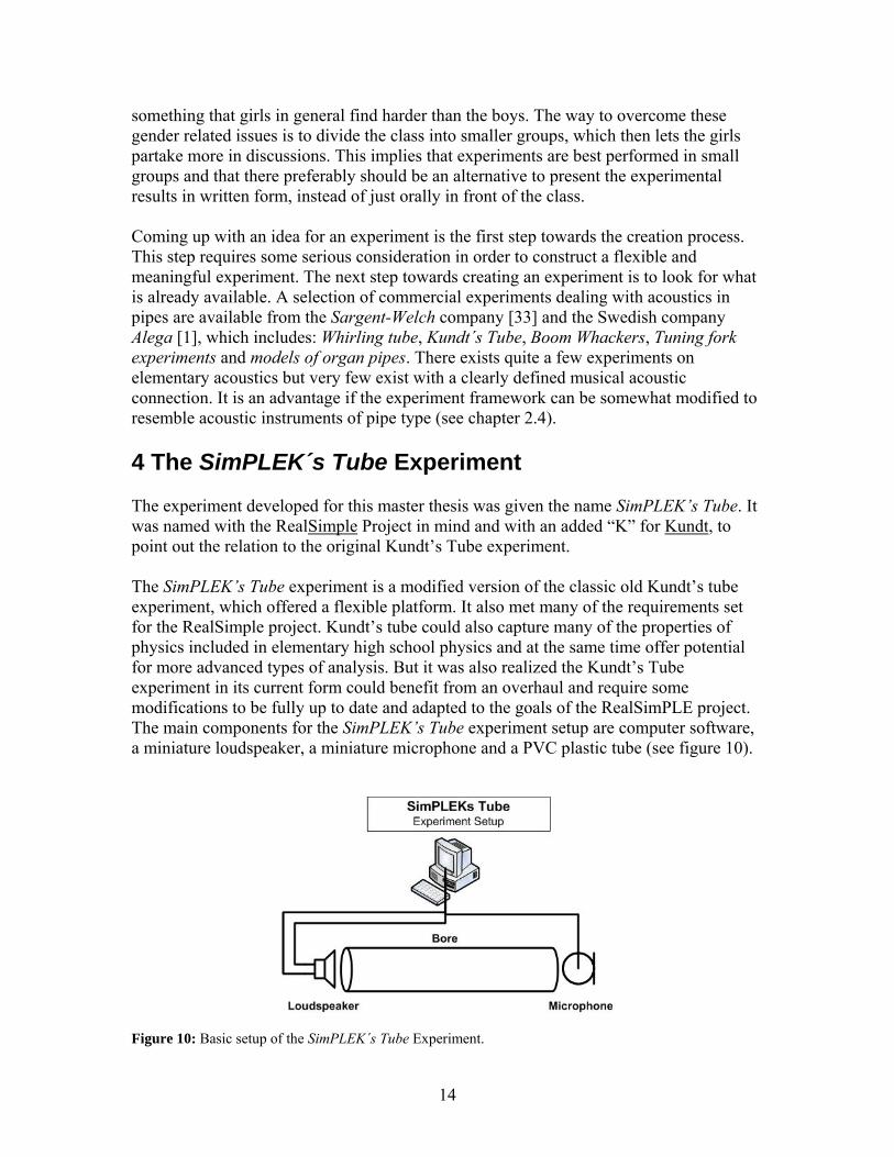
The experiment developed for this master thesis was given the name SimPLEK’s Tube. It was named with the RealSimple Project in mind and with an added “K” for Kundt, to point out the relation to the original Kundt’s Tube experiment. The SimPLEK’s Tube experiment is a modified version of the classic old Kundt’s tube experiment, which offered a flexible platform. It also met many of the requirements set for the RealSimple project. Kundt’s tube could also capture many of the properties of physics included in elementary high school physics and at the same time offer potential for more advanced types of analysis. But it was also realized the Kundt’s Tube experiment in its current form could benefit from an overhaul and require some modifications to be fully up to date and adapted to the goals of the RealSimPLE project. The main components for the SimPLEK’s Tube experiment setup are computer software, a miniature loudspeaker, a miniature microphone and a PVC plastic tube (see figure 10).

Figure 10: Basic setup of the SimPLEK´s Tube Experiment.

14

4.1 Bore model The tube of the experiment was modeled to resemble that of the resonator/bore of an acoustic instrument. For this a piece of PVC plastic tube, normally used for electrical installations was used (see figure 11). The PVC tubes can be found at low cost in regular hardware stores, in lengths of two meters and with a choice of two diameters, 18 and 20 mm. The tube used in this experiment is the 20 mm diameter type, which exactly fits the excitation device described in chapter 4.2

Figure 11: PVC plastic tubing used in the experiment (image from www.elfa.se). The bore was divided into two separate segments (40 respectively 20 cm) to enable adjustable tube length. To model the effect of tone holes, two holes were drilled on top of the PVC plastic tube. These holes measured 8 mm in diameter and were placed strategically to ensure that the users of the experiment could experience the effect of a tone hole, placed both on an air pressure node and on an anti-node. The two tube sections were attached to each other with either electrical tape or with a plastic connector-piece designed for attachment of PVC tubes (see figure 12). The latter of these two solutions offers more flexibility since the two tube sections can be fitted and refitted without any obtrusions as in the case of using tape. For more exact description on how to perform the assembly, see appendix Construction Manual.

Figure 12: Attachment material options for the PVC plastic tubing, connector (left) and electrical tape (right) (images from www.elfa.se).

4.2 Source of Excitation For this experiment two different sources of excitation were used. The first excitation source used for this experiment was a miniature loudspeaker manufactured by Fabr Veco Vansonic. Its diameter precisely matched the one of the PVC plastic tube, which made assembly straightforward. Further, the impedance of the miniature loudspeaker allowed it to be driven solely from a sound card, without an external amplifier. As a tradeoff from the small dimension characteristics of the loudspeaker, its frequency range and output power are somewhat limited. More details on assembly of the loudspeaker unit are given in appendix Construction Manual.

15

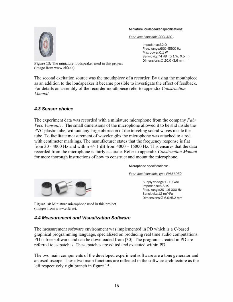
Figure 13: The miniature loudspeaker used in this project (image from www.elfa.se).

Miniature loudspeaker specifications: Fabr Veco Vansonic 20CL32G . Impedance:32 Ω Freq. range:600–5500 Hz Max power:0.1 W Sensitivity:74 dB (0.1 W, 0.5 m) Dimensions:∅ 20.0×3.6 mm

The second excitation source was the mouthpiece of a recorder. By using the mouthpiece as an addition to the loudspeaker it became possible to investigate the effect of feedback. For details on assembly of the recorder mouthpiece refer to appendix Construction Manual.

4.3 Sensor choice The experiment data was recorded with a miniature microphone from the company Fabr Veco Vansonic. The small dimensions of the microphone allowed it to be slid inside the PVC plastic tube, without any large obtrusion of the traveling sound waves inside the tube. To facilitate measurement of wavelengths the microphone was attached to a rod with centimeter markings. The manufacturer states that the frequency response is flat from 30 - 4000 Hz and within +/- 1 dB from 4000 – 16000 Hz. This ensures that the data recorded from the microphone is fairly accurate. Refer to appendix Construction Manual for more thorough instructions of how to construct and mount the microphone.

Figure 14: Miniature microphone used in this project (images from www.elfa.se).

Microphone specifications: Fabr Veco Vansonic, type PVM-6052. Supply voltage:1–10 Vdc Impedance:5.6 kΩ Freq. range:20–16 000 Hz Sensitivity:12 mV/Pa Dimensions:∅ 6.0×5.2 mm

4.4 Measurement and Visualization Software The measurement software environment was implemented in PD which is a C-based graphical programming language, specialized on producing real time audio computations. PD is free software and can be downloaded from [30]. The programs created in PD are referred to as patches. These patches are edited and executed within PD. The two main components of the developed experiment software are a tone generator and an oscilloscope. These two main functions are reflected in the software architecture as the left respectively right branch in figure 15.

16

Figure 15: Flowchart of the measurement/visualization software architecture. A further reflection of the two signal paths is the base structure of the software visualized is seen in figure 16. The left structure initiated by a [adc~] block handles the incoming data from the microphone (for an explanation of building blocks available in PD see [38]). Incoming data are then filtered in order to remove unwanted frequencies. Then the data is sent to two separate units that calculates the FFT for displaying the spectrum and secondly a trigger module for displaying the waveform. The right structure terminated by a [dac~] block produces the signal fed to the loudspeaker. It features four cosine oscillators together with an additive synthesis module. PD offers the possibility of creating substructures named sub-patches within a building block. A number of objects can be encapsulated into one sub-patch block and thus make the overall structure easier to understand. This was used for the FFT block, trigger block, the separate oscillators and the additive synthesis.

Figure 16: The main PD patch for the measurement software (sub-patches indicated by an initial pd argument)

17

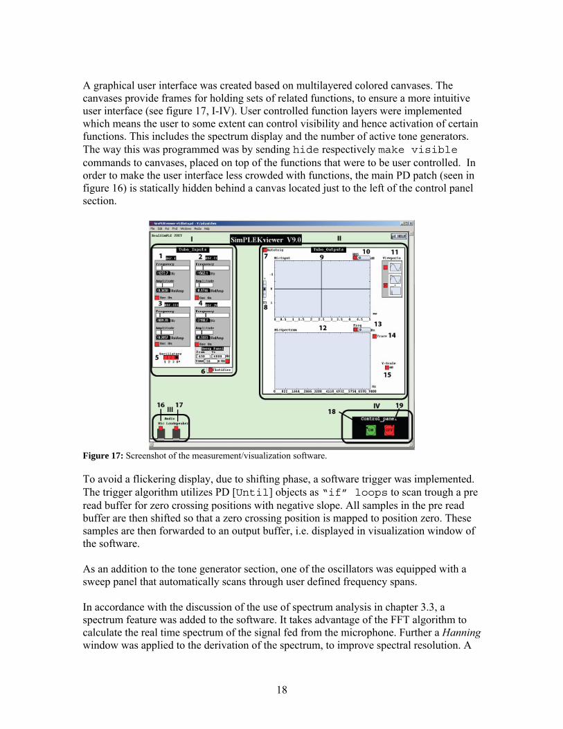
A graphical user interface was created based on multilayered colored canvases. The canvases provide frames for holding sets of related functions, to ensure a more intuitive user interface (see figure 17, I-IV). User controlled function layers were implemented which means the user to some extent can control visibility and hence activation of certain functions. This includes the spectrum display and the number of active tone generators. The way this was programmed was by sending hide respectively make visible commands to canvases, placed on top of the functions that were to be user controlled. In order to make the user interface less crowded with functions, the main PD patch (seen in figure 16) is statically hidden behind a canvas located just to the left of the control panel section.

Figure 17: Screenshot of the measurement/visualization software. To avoid a flickering display, due to shifting phase, a software trigger was implemented. The trigger algorithm utilizes PD [Until] objects as “if” loops to scan trough a pre read buffer for zero crossing positions with negative slope. All samples in the pre read buffer are then shifted so that a zero crossing position is mapped to position zero. These samples are then forwarded to an output buffer, i.e. displayed in visualization window of the software. As an addition to the tone generator section, one of the oscillators was equipped with a sweep panel that automatically scans through user defined frequency spans. In accordance with the discussion of the use of spectrum analysis in chapter 3.3, a spectrum feature was added to the software. It takes advantage of the FFT algorithm to calculate the real time spectrum of the signal fed from the microphone. Further a Hanning window was applied to the derivation of the spectrum, to improve spectral resolution. A

18

Hanning window is generally a good choice of windowing function as it does not introduce more than a moderate amount of unwanted side lobes as a tradeoff [32]. An additional feature of the developed software spectrum visualization module is the trace function. The trace function makes the spectrum display to show the last value, detected at each frequency. This function allowed the user to see a complete system frequency response. This is especially valuable when performing a frequency sweep to detect resonances. To further emphasize the music acoustic connection in this experiment and to enhance user interactivity, a simple additive flute synthesis was added to the software module. The part that is interactive is that the user can adjust how many oscillators they want to use additively and of what frequency and amplitude. Trying to synthesize a realistic flute sound requires odd harmonics and noise [25]. In reality you would need about 40 harmonics to completely produce all such within in the human hearing range. That would make the synthesis processor intense. But judged experiences have indicated that six harmonics suffices to produce an average quality sound (also visible when comparing the relative amplitude of the harmonics in figure 3 and 4). To accomplish a fuller sound in the software module, two extra oscillators was added with frequencies determined by the difference of the third and fourth oscillator. Only summing up noise and generated cosine/sine waves proves to be a poor sounding solution, since the result sounds as two separate components. To better blend noise and oscillator together some modifications needs to be undertaken. The first thing to do is to tonally color the noise. That was done by band-pass filtering the noise at frequencies where the cosine-wave has harmonics. To further enhance the blending of noise and body sound, the timing needs to be adjusted. In a real flute you first hear a strong noise component followed by the body of the sound. This was achieved by applying amplitude modulation with two separate ADSR amplitude envelopes. One assigned for the sum of the oscillator components and one for the noise (envelopes displayed in figure 19). The ADSR envelopes were programmed using the internal PD [adsr~] argument. The noise was then also high-pass filtered to slightly increase the presence of its high frequency components. Finally some reverb was added from PD´s internal [rev3~] algorithm. The dry noise and oscillator-sum signals were fed to the reverb, which outputs a 20% wet signal. The wet signal with added reverb was then later mixed with the original dry signal and fed to the output. Ideally a flute synthesis includes more components such as vibrato, tremolo and some other processing to further increase the mirroring of a real flute. Teachers in general do not tend to like demonstrations of processes referred to as black boxes i.e. processes featuring components that does something that are too complex to explain to students. Due to this reason the number of complex steps in this additive synthesis algorithm was kept to a minimum, so the students can understand what they are doing. A detailed

19

description of the functions in the developed visualization software is available in appendix Software Instructions.

Figure 18: Additive flute synthesis software architecture featured Figure 19: ADSR amplitude

envelopes in the additive flute synthesis.

in the SimPLEK´s Tube experiment..

4.4 Applications of the SimPLEK´s Tube The SimPLEK´s Tube experiment can be used for investigating acoustical phenomena that occur when sound passes through a cylinder shaped cavity. The main area for the experiment setup is demonstrating resonance and how resonance frequencies relate to tube length. But it also can display how the placing of tone holes along a tube and alternatively opening them or covering them affects the amplitude of different frequencies. There is also the possibility of determining the speed of the sound by setting a frequency and then physically measuring the wavelength. With the oscilloscope auto trigger mode set to off, it is also possible to look at what happens to the waveform when the frequency is set on or near a resonance frequency. This is a way of briefly showing the effects of standing waves. The experiment can also be used for investigation of more basic properties like demonstrating how a sound wave appears in an oscilloscope and also for demonstrating the properties: amplitude, period, wavelength, node, anti-node and frequency and their respective relations. The software spectrum display can be used to analyze more complex sounds that consist of more than one frequency and for simplifying the process of finding different resonance frequencies. In its current configuration the experiment setup provides the users a brief introduction to additive synthesis and also the possibility to see how the parameters: amplitude, frequency and number of harmonics influences the result of the additive synthesis.

20

It is also possible to use this experiment without the accompanying software and instead use it together with an oscilloscope and a tone generator. With some small improvements as suggested in section, 8.2 Future Work, the experimental setup can also be used for more advanced types of acoustic analysis suited for college education. For examples of how the SimPLEK´s Tube experiment can be conducted see appendix Lab Instructions.

5 Web Portal

The first idea was to present the experiments created during this project on the Rice University web portal. However during the project it was realized that such presentation could entail difficulties for teachers to find information amongst the vast number other information presented on that site. After some discussion with team members of the RealSimPLE project, the decision was made to produce a dedicated Swedish project site. It was also decided that this task was to be included in this master thesis. The program used for creating the web portal was Macromedia Dreamviewer 8. Before designing a webpage it is useful to look at commercial websites for inspiration. For this project the inspiration was gathered from professional pages like www.kth.se, www.adobe.se and www.sony.se. After viewing these pages it was noticed that a minimalistic design works better as it does not draw attention away from what is being presented. Overall requirements for a website in general is that it is supposed to be intuitive, informative, interesting, and provide some form of interactivity [22]. One of the most common designs of web pages is nested tables i.e. putting table objects inside table objects [8]. This gives a flexible framework for grouping and formatting information. This is why this type of design was used for creating the web portal. The information was produced both in American English and Swedish, since the project is a cooperation between Stanford University and KTH. When choosing what information that is to be presented, two factors needs consideration [22]. “Which kind of information needs to be displayed for communicative reasons and which type of information is your user group really interested in”. The first thing that usually catches the eye of a viewer is the top banner. The thought behind the banner designed for this web portal was that it is supposed to briefly suggest to the viewer what he/she can expect from the site. In the case of the developed banner the user can get the information about the following: name of the project, who develops RealSimPLE and finally the acoustic connection (vaguely suggested by the sine pattern). To further specify what is being presented, images were added just below the top banner. The images are sets of photos taken when students perform the SimPLEK´s Tube experiment and the Monochord experiment (another RealSimple experiment). One further way of arousing interest is asking rhetorical questions. This is the idea for the text content that was presented on the start page of the web portal. The presented

21

information itself is also viewed easier if it is structured. This was done by separating the text into sections with headers and sub headers. To further make viewing simpler the contents of each page was kept within the length of the standard screen resolution height (1024*768), so there is no need for scrolling which makes it harder to get an overview. Since the project is going to continue to evolve the web portal needs to be flexible and easy to edit at later stages. To make future editing easier the web site was formatted using css2. This ensures future changes like choosing other fonts or styles are straight forward to perform, in one step and also applicable to the whole web portal [8]. Navigation on the portal was implemented as a single side navigation bar. To make a navigation bar more intuitive it is important to introduce some mouse rollover effect. It is tempting with good looking image rollovers but it is considered more practical with animated css text navigation style. Animated css style was chosen due to these reasons and the fact that later changing the contents is made easier and that the page loading time shortens. Also important is to inform users about updates or changed contents [22]. This can be done by putting an updated date stamp or a news section on the web portal. But since the portal is not going to be updated on a daily basis it seemed more appropriate to use a news section. Another important feature to attend to is to allow users to provide feedback [21]. This feature was implemented as a user forum where teachers can discuss their experiences from the experiments and suggest modifications. All tests of the web portals appearance in a web browser was made in both Microsoft Internet Explorer and Mozilla Firefox to ensure that all users see the information as intended. For a screenshot of the start page of the RealSimple web portal see figure 20.

2 In web development, Cascading Style Sheets (CSS) is a stylesheet language used to describe the presentation of a document written in a markup language. Its most common application is to style web pages written in HTML and XHTML, but the language can be applied to any kind of XML document, including SVG and XUL.CSS is used by both the authors and readers of web pages to define colors, fonts, layout, and other aspects of document presentation [22].

22

Figure 20: Screenshot of the start page from the website created for the Swedish part of the RealSimPLE project.

6 Experiment Evaluations

The experiment was evaluated from two perspectives, accuracy in how well it modeled the actual acoustics in pipes and subjectively from a user point of view. First the produced resonance frequencies were compared to theoretically calculated ones. Then a frequency response of the experiment was evaluated in terms of amplitude. Finally some opinions from teachers on usability of the experiment are presented.

6.1 Model Performance For the evaluation of the accuracy of the models resonance frequencies, values of resonance frequency were read as closely as possible from spectrum software display during a frequency sweep. This was done both for the 40 cm tube and the extended 60 cm tube. Tape was used during measurements to seal the tone holes so no air could slip through. The conditions were otherwise as intended for the standard procedure of the experiment. These values were then compared with values theoretically calculated using the formula for open-closed tube (expression 7) combined with adjustment (expression 10) for effective tube length (see table 1 and 2 for results).

23

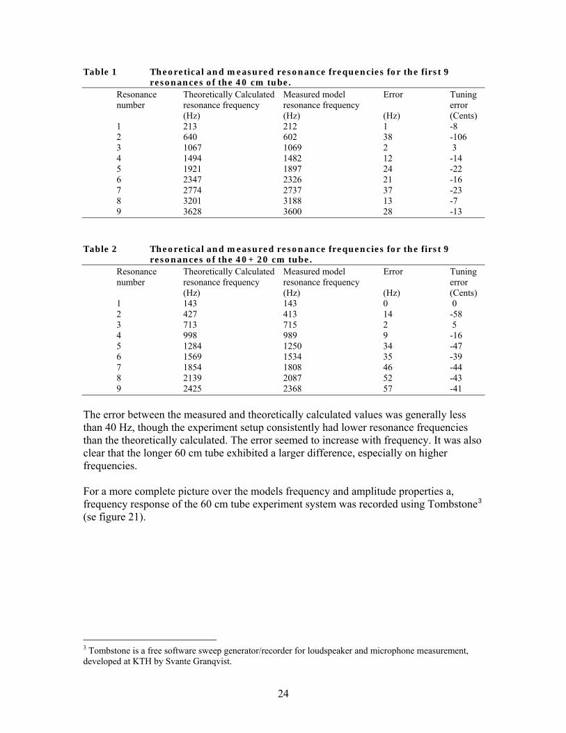
Table 1 Theoretical and measured resonance frequencies for the first 9 resonances of the 40 cm tube.

Resonance Theoretically Calculated Measured model Error Tuning number resonance frequency resonance frequency error

(Hz) (Hz) (Hz) (Cents) 1 213 212 1 -8 2 640 602 38 -106 3 1067 1069 2 3 4 1494 1482 12 -14 5 1921 1897 24 -22 6 2347 2326 21 -16 7 2774 2737 37 -23 8 3201 3188 13 -7 9 3628 3600 28 -13

Table 2 Theoretical and measured resonance frequencies for the first 9

resonances of the 40+ 20 cm tube. Resonance Theoretically Calculated Measured model Error Tuning number resonance frequency resonance frequency error

(Hz) (Hz) (Hz) (Cents) 1 143 143 0 0 2 427 413 14 -58 3 713 715 2 5 4 998 989 9 -16 5 1284 1250 34 -47 6 1569 1534 35 -39 7 1854 1808 46 -44 8 2139 2087 52 -43 9 2425 2368 57 -41

The error between the measured and theoretically calculated values was generally less than 40 Hz, though the experiment setup consistently had lower resonance frequencies than the theoretically calculated. The error seemed to increase with frequency. It was also clear that the longer 60 cm tube exhibited a larger difference, especially on higher frequencies. For a more complete picture over the models frequency and amplitude properties a, frequency response of the 60 cm tube experiment system was recorded using Tombstone3 (se figure 21).

3 Tombstone is a free software sweep generator/recorder for loudspeaker and microphone measurement, developed at KTH by Svante Granqvist.

24

Figure 21: Frequency response of the experiment setup. Data displayed in a logarithmic scale, using the 60 cm tube. Data recorded in Tombstone. Analysis of the frequency response showed large amplitude anomalities, especially visible below 700Hz and around the area of 2500Hz. Since the loudspeakers lower frequency range is set at 600Hz this was to be expected. The amplification of the frequencies around 2500Hz was probably also a result of the performance of the loudspeaker.

6.2 Focus group results The experiment was subjected to evaluation in form of discussions and a questionnaire (see appendix Questionnaire) that involved teachers at high school. Five high school teachers from Kärrtorps Gymnasium4 within the area of physics and technology tried the experiment and discussed it freely and with respect to questions found in the questionnaire. This discussion revealed several facts of interest for the development of the experiment. One problem with conducting the experiment is the availability of computers in schools. Many computers are placed in computer lecture rooms which are troublesome to book for lectures in physics, due to high usage. However the situation is slowly improving as more and more physic lecture rooms gets access to computers and projectors. The budget physic teachers are restrained to for buying education equipment is very limited. Usually granted funds for equipment like computers and experiments need to last for as long as

4 Kärrtorps Gymnasium is an upper secondary school, focused on IT and media, located in Stockholm.

25

five years. This fact rendered it important to the make sure that the experiment can run on older computers. It is important that the introduction of the lab instructions provide a solid connection to the course literature. That is so the teacher can relate the subject of the experiment with specific chapters in the course literature. Properties of interest to demonstrate in experiments are all that are closely related to the properties found in the chapters of the course material (see chapter 3.2 for a specification). The general idea of the RealSimPLE project to combine computer measurements with a physical model and simulations was perceived as a really interesting concept. Another aspect that was found appealing with the experiment was the focus on low cost. This is vital since that makes it possible to buy material for a class setup. Some teachers were enthusiastic about the concept of using accessible low cost materials and saw potential in using them for other types of experiments like for example demonstrating interference. Especially the miniature loudspeaker and microphone seemed to offer a flexible framework for construction of experiments. Commercial experiments that are used today in education are costly to purchase and the range of available experiment is limited. Everyday use of experiments from high school students tends to wear down the experiments fairly quick, which requires constant purchases of spare parts. These parts are in general costly and hard to find some years after the original purchase of a commercial experiment. Inquiries about lack of spectrum in the course plan for physics on high school revealed that some teachers actually introduce spectrum, in order to clarify properties of sounds that contains more than one frequency component. The course literature used in physics education on high school is usually one of two widely spread textbooks. These are: Quanta B [11] and Heureka! Fysik för Gymnasiskolans Kurs B [6]. The webpage which hosts the experiment was found informative and also easy to navigate on and finding relevant information.

7 Discussion and Conclusions

The developed experiment SimPLEK’s Tube which basically is a modification of Kundt’s Tube was successful on several accounts. An evaluation from potential users i.e. teachers at high schools indicated that the experiment is ready to put in immediate use. A functional web portal is also up running. The first plan was to put all material on a general web portal run by Rice University, but as the project progressed it was realized that a dedicated Swedish project web page would be more appropriate for distribution of the material. The material is more accessible in this way instead of browsing through

26

many pages on a general portal when trying to find information about the RealSimPLE project. Comments from teachers about what they liked/disliked about the experiment further revealed that the first hand impression of the experiment is mainly a positive one. Comments included: - Flexibility – In building own models especially since the software PD lets users fairly easy modify or construct own modules. - Commercial experiments tend to be expensive compared to RealSimPLE experiments and it is hard to find spare parts. - RealSimple experiments integrate software and hardware, often one of these is left out. - Interesting with the musical instrument connection, enables integration with music teaching. - One problem is that the availability of computers in physic lecture rooms, which varies greatly among different schools. The development in schools today goes towards more and more possibilities of computer based education. The overall challenge during this thesis was not creating a complex technical solution. It was merging all parts together to form an accessible, interesting and useful experiment. The main ambition for the RealSimPLE project is that the developed experiments will be used in schools. That means it had to compete with commercial products. For this to work the created experiment had to do something better the commercial ones. The first objective in the development of any experiment is coming up with an idea for the actual experiment. First looks at existing products such as classic and commercial experiments were a great idea for receiving inspiration, for the creation of a new experiment. Experiments of special interest were those that presented as many acoustic properties as possible in a straight forward way. Also of interest were experiment platforms that displayed similarities to acoustic instruments, in order to establish the musical acoustic connection. Kundt’s Tube was one of those that seemed to have potential. It fulfilled the requirement of offering demonstrations of acoustics in pipes and the possibility of being modified to resemble acoustic instruments. Secondly making the software functional and user-friendly was also a challenge. Important here was to attempt to minimize the number of necessary function and to ensure each function had enough space in the user interface. These problems were solved by separation of function categories by frames and implementing some user level layer controlled functions i.e. functions that the user can activate depending of needs. It would have been favorable if PD had more flexible ways of presenting and importing media. The developed GUI could then have been made more appealing and intuitive. PD vector handling made it difficult to produce a stable trigger for the software oscilloscope. The problem was to find a way of detecting a trigger point, by searching through a vector of input values and then shifting those samples. If one attempted to do this fast using [metro] objects, the output skipped shifting some values which rendered

27

in a poorly updated display. The issue was finally solved by replacing a [metro] object with an [until] object. Viewed as a pedagogic challenge the project needed some consideration in order to produce a useful result. As stated in chapter 3 the key to achieving this was to present a clear purpose, that is suggest to the students what they can learn from the experiment. The next step was trying to create tasks that offer variation, so that the students are motivated to continue with the experiment. Further it was very important to try and connect the experiment to something that the students already are familiar to, for example familiar sounds. By doing that it makes it easier for students to understand, as they can relate to something that already is familiar to them. Also students then easier realize what the new knowledge can be used for. It is often the case that demonstration of physics offers a simplified version rarely seen in reality, as the mathematics of reality in general is quite advanced. There is however a danger in demonstrating simplified versions of reality, which seriously threatens to reduce the motivation of the students. This implicates that there is always a tradeoff between how accurate models you can demonstrate and how complex mathematical explanation will be accepted. All tasks of the experiment also had to be adapted to the right complexity level, which in this case is to the subjects taught by the teachers and the course literature. The final goal of all considered pedagogic aspects was to get the student to experience moments of insight. All these pedagogic aspects have influenced the construction of the experiment and especially the experiment instructions and the different tasks of the experiment. The choice of parts for the experiment was also an area for consideration. The main issue was the choice of excitation device. The choice finally fell on a cheap miniature loudspeaker. This was beneficiary for reducing the cost of the experiment and also the assembly process, but it made it rather difficult to detect the first two resonance frequencies. That did however not motivate the choice of a better loudspeaker since that would implicate the need of external amplification, which greatly would have increased the total cost of the experiment. As a late addition to the experiment, the decision was made to add a further excitation source. The reason for this was to introduce a more realistic flute model, which included feedback. The second excitation source consisted of the mouthpiece of a recorder. However when trying to implement a feedback controlled excitation source, problems occurred. The sound pressure level in the tube when using the recorder mouthpiece got very high and created signal saturation. This problem was finally overcome by introducing a damping section for the microphone. Another time consuming task during the project was creating all documentation. Especially since changing one thing in the experiments meant one had to change the documentation parts in several documents, both in Swedish as well as in English In general, though, the developed experiment did not meet all the goals set for this master thesis. One of the goals that were not achieved was to make it adapted both for High school and College. As the project progressed it was decided that the main goal should be to first produce a working product for high school. Then later from that point improve the experiment if there was enough time. Some early experiments with such an adaptation for

28

college level is suggested and presented in chapter 8.2 Future Work. Further the goal of introducing Stanford simulations into the software was also not reached. This would have required Stanford having access to the experiment specifications, on an earlier stage of the project. The primary test of the correctness of the experiment in this instance was the comparison of its resonance frequencies with the theoretically calculated ones. The secondary test of the experiment was the analysis of its frequency response. Both these tests showed that the model was somewhat deficient in the respect of frequency and amplitude. Both these discrepancies could to a large extent mainly be seen as a result from the performance of the miniature loudspeaker. This implicates that finding the first set of resonances requires amplitude to be maximized, for detection. Also it means that amplitude needs to be adjusted around frequencies in the 2500Hz area, to avoid saturation. Since the focus in this project was not mainly set on exact reproduction of acoustics, but rather more on finding a way of demonstrating acoustics, these errors can be tolerated. Ultimately, the undertaking of creating an experiment with both software and hardware modules requires background in acoustics and related fields, some experience from programming and also preferably some knowledge of pedagogy. It was quite easy to forget that technical understanding is on a completely another level in high school, especially when you have studied many years. You tended to forget what is easy and what is hard to understand. Feedback from teachers and students were therefore very useful. Even more useful was the experience of having worked as a teacher. One advice for future projects concerning the creation of RealSimPLE experiments is to involve teacher and students on an earlier stage. It would also have been a good idea to initiate the cooperation part with Stanford earlier. The problem here was that one wants a relatively complete experiment, before presenting it in front of teachers or to sending it for computer modeling. To present complete specifications was hard on an early stage of the project. More extensive user feedback had also been ideal. This was however difficult to achieve due to the fact that teacher are quite busy and plans their educations for months ahead. As a closing statement I would like to add that performing this master thesis was inspiring. It offered challenges on many areas like web programming, software programming, technical construction, writing technical manuals and meetings with potential users. These widely spread areas offered an excellent way of testing the knowledge gained during several years of civil engineering education.

29

8 Future Work

8.1 Minor Improvements To investigate why certain instruments have a bell shaped end section, one could switch the extension tube section to a funnel, resembling a trumpet cone. Another interesting experiment is to switch the extension tube for a curved one. This would shed some light on what happens in certain instruments like for example trumpets, which have curved tubing sections. Both these objects the funnel and the curved tube can be found for a small cost, about $2 and can easily be mounted without any modification on the experiment setup.

Figure 22: PVC tube extension piece alternatives (curved tube left, funnel right), (images from www.fredells.com) Adding a simple noise generator to the software module can be a good idea, so students during the beginning of the experiment can get a better understanding of properties like: sound components, frequency and spectrum. Both the speaker and the microphone input and output levels are dependent on volume settings in the OS. This implicates the user often has to adjust these settings for the experiment, as every user have their own specific settings tuned. Otherwise saturation can arise in the loudspeaker, microphone or in the sound card. This especially poses a problem since the amplitude rise to relatively high levels during resonance. A nice workaround for this would be to implement some form of automatic volume/amplitude adjustments in the software. To add general sound card support would be a great improvement. Some Realtek soundcards found in laptops with built in microphone do not support the current microphone hardware configuration of the experiment. This could probably be solved by instructing users with a Realtek sound card, to mount an external power supply like a battery. Another fix to implement is to stabilize the trigger function in the software. On rare occasions directly on start-up the trigger stops functioning and the display shows nonlinear curves instead of sine waves. This is always solved by restarting the computer, but since that consumes some time it would be better to find a solution for this issue.

30

8.2 College Level Extension In the current configuration, the experiment SimPLEK’s Tube is intended for high school level. It would be of great interest to improve, so it also could be used in college education. A conceivable approach here is to work on two key areas. The first key area would be to develop more experiments using the recorder mouthpiece. As this was a late addition to the experiment, only a few tasks in the experiment include using the mouthpiece. But as it offers more realism, it could be used for more advanced types of measurements. The second key area to attend to would be to add software modules for more advanced types of acoustic analysis. Two possible options here would be to introduce measurements of the acoustic impedance and the impulse response. This could be done without any major changes to the experiment setup, using methods as described in [40], or more in depth in [5]. Some initial experiments with adding an impulse response module to the software for SimPLEK’s Tube showed favourable results (see figure 23 on the next page). The experiment was done using a triangular impulse generated in PD and about four samples long. The issue here was to shorten the impulse length since its ideal length would be one sample. That did however not prove to be easy to implement. Neither sampling a Dirac pulse nor internally generating an impulse worked. The next issue to address here was to program a trigger that displays the impulse satisfactorily. Another beneficial enhancement would be to add Stanford simulations to the software, module as soon as they are finished. This would primarily serve two purposes: the possibility to compare results from the simulations with the results of the physical model; and provide the option to choose from different flute synthesis techniques, other than the additive method that exists in the software today.

31

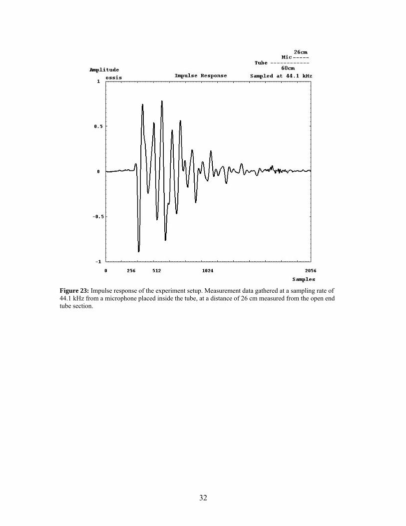
Figure 23: Impulse response of the experiment setup. Measurement data gathered at a sampling rate of 44.1 kHz from a microphone placed inside the tube, at a distance of 26 cm measured from the open end tube section.

32

References

[1] Alega Skolmaterial AB. Website*: http://www.alega.se/. 2007. [2] A. H. Benade. Fundamentals of Musical Acoustics. Oxford University press, New York, 1976. [3] A. H. Benade. “On the Propagation of Sound Waves in a Cylindrical

Conduit”. J. Acoust. Soc Am. 44. 616-623. 1968 [4] D. Benson. Music: A Mathematical Offering. University of Aberdeen,

Website*: http://www.maths.abdn.ac.uk/∼bensondj/html/maths-music.html. 2006.

[5] L. Beranek Acoustical Measurements. Acoustical Society of America,

Cambridge, 1988. [6] L. Bergström. et al. Heureka! Fysik för Gymnasieskolan Kurs B. Natur och Kultur, Viborg, 2005. [7] G. T. Chair. et al. Goals of the Introductory Physics. The Physics

Teacher, Vol. 35, Dec. 1997. [8] G. Chow. Macromedia Dreamweaver 8 Essential Training. Website*:

http://lynda.com, 2006. [9] Collegeboard.com Inc. Recommended High School Classes. Website*:

http://www.collegeboard.com/student/plan/high-school/106.html. Collegeboard.com Inc, 2007.

[10] J. W. Coltman. “Acoustics of the Flute”. Physics Today 21. 25-32. 1968. [11] B. Ekstig. Quanta B : Fysik för Gymnasieskolan. Natur och Kultur, 2004. [12] Encyclopædia Britannica 11th Edition. Website*: www.1911encyclopedia.org. [13] R. P. Feynman. The Feynman Lectures on Physics. Addison-Wesley,

Reading, 1964. [14] N. H. Fletcher. & T. D. Rossing. The Physics of Musical Instruments. Springer-Verlag, New York, 1998. [15] S. Gang. Decisive Factors in Teaching and Learning. The Physics

Teacher, Vol. 38, Oct. 2000. [16] D. Hall. Musical Acoustics An Introduction. Wadsworth publishing

Company, Belmont, 1980.

33

[17] H. Helmholtz. On the Sensations of Tone as a Physiological Basis for the

Theory of Music. Dover Publications, Inc., New York, 1954. [18] J. L. Hunt. Five Quantitative Physics Experiments (Almost) Without Special

Apparatus. The Physics Teacher, Vol. 43, October 2005. [19] A. Hirschberg. Mechanics of Musical Instruments. Springer-Verlag, 1995. [20] D. H. Keefe. Theory of the Single Woodwind Tone Hole. Journal of the Acoustical Society of America 72. 688-699. 1982. [21] KTH Research Project Database, REALSIMPLE - Combining physical

reality with simulations in pedagogical laboratory experiments. Website*:http://researchprojects.kth.se/index.php/kb_1/io_9536/io.html. 2006.

[22] E. Ladd. & J. O´Donnel. HTML, JAVA och CGI. Prentice Hall, UK, 1998. [23] M. Lazar. Let's Review: Physics. Barron's Educational Series Inc, New York,

2003. [24] K. Leimer. J. Wikström. Hur Fysiklärare gör Fysik Intressant för både

Pojkar och Flickor från Skolår sex till nio. Högskolan Kristiansstad, 2005. [25] H. Monson. Hayes. Statistical Digital Signal Processing and Modeling. John Wiley and Sons Inc. New York, 1996. [26] G. D. Moore. Physics of Music Lecture Notes. McGill University,

Website*: http://www.physics.mcgill.ca/~guymoore/ph224/lecnotes.ps. 2006.

[27] T. Moran. Applications of Sound Spectrum Analysis. The Physics Teacher, Vol. 45, February 2007. [28] Music Theory Expression Marks. Website*: http://library.thinkquest.org/

15413/theory/expression.htm. [29] M.W. Passer. & R.E. Smith. Psychology. The Science of Mind and Behavior. McGraw-Hill, New York, 2004. [30] M. Puckette. The Theory and Technique of Electronic Music. University of

California. Website*: http://www.crca.ucsd.edu/~msp/techniques/v0.02 /book-html/. 2006.

34

[31] RealSimPLE Project Website. Website*: http://www.speech.kth.se/ ~sten/realsimple/simple.html.

[32] G. Reid. Synth Secrets: Synthesizing Pan Pipes. Sound On Sound, August 2003. [33] Sargent-Welch, Website*: http://sargentwelch.com. [34] Science Teaching Reconsidered. How Teachers Teach: Specific Methods. Website*: http://www.nap.edu/readingroom/books/str/2.html. [35] R.A. Serway. J.W. Jewett. Physics for Scientists and Engineers with Modern

Physics, 6th edition. Thomson Brooks/Cole, Belmont, 2004. [36] Skolverket, Kursplan FY-1202 Fysik B. Website*:

http://www3.skolverket.se/ki03/front.aspx?sprak=SV&ar=0607&infotyp=5&skolform=21&id=3054&extraId=

[37] J. Sundberg. Musikens Ljudlära. Proprius Förlag, Stockholm, 1989. [38] The Pure Data Portal. Website*: http://www.puredata.org/ [39] J. O. Smith. Physical Audio Signal Processing: Digital Waveguide

Modelingof Musical Instruments and Audio Effects. Stanford University, Website*: http://ccrma.stanford.edu/~jos/pasp04/

[40] M. Walstijn. Discrete-Time Modelling of Brass and Woodwind Instruments

with Application to Musical Sound Synthesis. University of Edinburgh. Website*: http://www.ph.ed.ac.uk/~maarten/

[41] V. Välimäki. Discrete-Time Modeling of Acoustic Tubes using Fractional

Delay Filters. Helsinki University of Technology, Espoo Finland, report no. 37 1995.

[42] U. Zölzer. DAFX:Digital Audio Effects. John Wiley and Sons Ltd, West

Sussex, 2002. *Information from websites gathered during the period from 2006-12 till 2007-02

35

A Questionnaire

At the beginning of the project some students and teachers at college level were asked some questions regarding experiments on acoustics. The main reason for this was to receive some views on what teachers and students during experiments find useful and thought provoking, in order to make the experiment designed in this project more interesting and enlightening. The questions were: Is there any particular part of acoustic that are easy or hard to understand? What experiments are being conducted on acoustics today? How are they conducted? Pros and cons about these experiments? What makes an experiment meaningful and interesting? Which acoustic properties would you like to have demonstrated/visualized? (Standing waves, resonance, wave propagation, pressure, harmonics, nodes etc) Are there any lecture rooms with accessible computers available? Rate the following on a scale from one to ten: Cheap material is important? Ease of use is important? Graphic design is important? What textbooks and material is used in the education of acoustic? Pros and cons about these resources?

36

Construction Manual The SimPLEKs Tube

Where Simulation meets Reality

— there comes knowledge

37

Table of Contents

Material & tools ............................................................................................................ 39 Tools ......................................................................................................................... 39

Material ..................................................................................................................... 39 Assembly....................................................................................................................... 40

Loudspeaker .............................................................................................................. 40 Microphone ............................................................................................................... 40 Microphone damping kit........................................................................................... 41 Flowerstake ............................................................................................................... 42 Tube shaping............................................................................................................. 42 Recorder mouthpiece ................................................................................................ 43

Testing........................................................................................................................... 43 F.A.Q............................................................................................................................. 44

38

Material & tools The following tools and material are needed to construct the experiment setup:

Tools Saw (preferably jigsaw), soldering iron/station, power drill.

Material Material/components: Aproximate price:1 x PVC-tube* 3 $1 x PVC tube connector package (optional) 3 $1 x miniature loudspeaker** 2-5 $1 x Male plug mini-jack ∅3.5 mm, 3-pole. (1 x miniature microphone***) 3-5 $1 x Male plug mini-jack ∅3.5 mm, 3-pole. Or (1 preassembled miniature microphone) 30- $ 1 flowerstake 1 recorder 1 Straw Solder 1 x 10μF capacitor 1 sx 2K2 resistor Insulated wire, red and black Electrical tape

Totalt: 25- $ * Tubing: we used a PVC plastic tube of the kind used for electrical installations, with the inner diameter ∅20 mm and the outer diameter ∅22 mm. ** Miniature loudspeaker: Look for small dimensions and good characteristics. We used a Fabr Veco Vansonic 20CL32G . Try to find something similar. Impedance: 32 Ω Freq. range: 600–5500 Hz Max power: 0,1 W Sensitivity: 74 dB (0.1 W, 0.5 m) Dimensions: ∅ 20.0 × 3.6 mm Note that this speaker’s diameter fits snugly in the PVC tube. The impedance makes it easily driven. The lower limit of the frequency range should be as low as possible.

39

*** Microphone: We used a Fabr Veco Vansonic, type PVM-6052. Try to find something similar. Supply voltage: 1–10 Vdc Impedance: 5.6 kΩ Freq. range: 20–16 000 Hz Sensitivity: 12 mV/Pa Dimensions: ∅ 6.0×5.2 mm Soundblaster-compatible sound cards generally supply a 5 V voltage through the microphone input connector. This is well within the microphone specs. No external power supply is necessary.

Assembly Assembly is done in three steps: loudspeaker, microphone and the tube. Assembling the experiment should take about 1 hour.

Loudspeaker Cut two pieces of electrical wire of the length that is required to reach from the sound card input connector to the placement of the experiment setup. Remove 2-3 mm of insulation from all 4 ends of the cables.

Unscrew the metal case of the miniplug.

Now solder one of the loose ends of the cable to the tip terminal (left channel) of the mini-jack and the other to the sleeve terminal (ground). Leave the (middle) ring terminal unconnected - otherwise the right channel output of the sound card will be short-circuited, possibly resulting in damage. Wind some electrical tape around the solder to avoid contact with the case. Pull the loose end of the wires through the metal case. Screw the metal case back on. Solder one end of each wire to the connectors of the miniature loudspeaker. Wind some electrical tape around the soldered points to protect them.

Microphone If you have bought a preassembled Microphone, skip to the last paragraph of this section. The length of the microphone cable needs to exceed the distance from the computer sound card input to the position of the tube by about half a metre, so that the microphone

40

may also be inserted into the tube. Remove 2-3 mm of insulation from all 4 ends of the cables.

Unscrew off the protective metal case Solder a black wire to the longest pin (Sleeve). Solder the longer leg of the capacitor to the Tip pin (in the middle of the insulated area). Solder the resistor to the pin that is left over (Ring). Solder a red wire together with the free ends of the capacitor and the resistor. Put small pieces of tape on the legs of the components, to protect from short-circuits. Screw the metal case back on. Important: thread the cables thru the contacts metal case before you solder the microphone! Solder the two loose ends of the cable you just attached to the plug onto the two connectors of the microphone. Wind some tape around the connection between mic. and wires and between the wires and the plug so that they do not break from bending back and forth. Hold one end of the cable at a position just before the tape you just put there and grip the other end of the cable just before the plug and while stretched spin one end while holding the other still. This makes the cables intertwine and hold together like a braid. You can repeat the same procedure with the loudspeaker cables. The spiraling wire makes the lead less sensitive to electrical interference.

Microphone damping kit A damping kit for the microphone is necessary when measuring on the recorder mouthpiece. This is because of the high SPL levels that arise inside the tub. Cut a 2 cm piece of a straw. Use a straw of diameter that can be thread onto the miniature microphone. Make a roll of tape that fits inside the straw. Put the roll inside the straw and make sure a tight fit. Seal that end by wiring some tape around it.

41

Flowerstake To facilitate measurements later, make centimeter markings along the flower stake. Attach the microphone at the end of the stake with insulating tape.

Tube shaping 1. Saw two pieces of PVC plastic tube. One piece should be 40 cm long and the other, 20 cm. Smoothen the rough edges to ensure a tight fit.

2. Tape the two pieces together using the electrical tape. Wrap around position 1. Alternatively, use one of the PVC plastic tube connectors if you have chosen to buy those. 3. Drill one 8 mm diameter hole at 9.4 cm from the end of the shorter tube section (position 1), and a second 8 mm diameter hole at 23 cm from the end of the shorter tube section (position 2. Smoothen the rough edges of the holes with a knife. Cover the holes with a small piece of electrical tape. The tape will be taken on and off during the experiments. An alternative to the tape is to two cut two pieces of the connectors and use them as cover of one for each hole. 4. Attach the miniature loudspeaker at the beginning of the longer section (position 1). Secure the cable with electrical tape so that it does not bend back and forth in normal use. Also cover the backside of the loudspeaker with a several layers of tape, so as to seal the end of the pipe.

42

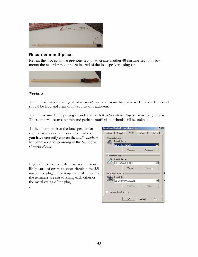
Recorder mouthpiece Repeat the process in the previous section to create another 40 cm tube section. Now mount the recorder mouthpiece instead of the loudspeaker, using tape.

Testing Test the microphone by using Windows Sound Recorder or something similar. The recorded sound should be loud and clear with just a bit of headroom. Test the loudspeaker by playing an audio file with Windows Media Player or something similar. The sound will seem a bit thin and perhaps muffled, but should still be audible. If the microphone or the loudspeaker for some reason does not work, first make sure you have correctly chosen the audio devices for playback and recording in the Windows Control Panel: If you still do not hear the playback, the most likely cause of error is a short-circuit in the 3.5 mm stereo plug. Open it up and make sure that the terminals are not touching each other or the metal casing of the plug. .

43

F.A.Q 1. F: S:

44

The SimPLEKs Tube

Where Simulations meet Reality

— There is knowledge

Software Manual

45

RealSimPLE 2007

Table of Contents

System Requirements 1 Installation Instructions 1 Connecting the Tube Model 1 Running the Experiment 1 Software Function Overview 2 Software Details 3 Troubleshoot 4

46

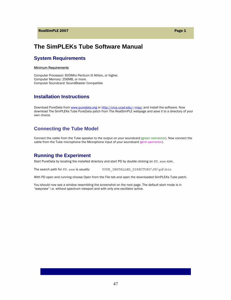
The SimPLEKs Tube Software Manual

System Requirements Minimum Requirements Computer Processor: 600Mhz Pentium III Athlon, or higher. Computer Memory: 256MB, or more. Computer Soundcard: SoundBlaster Compatible

Installation Instructions Download PureData from www.puredata.org or http://crca.ucsd.edu/~msp/ and install the software. Now download The SimPLEKs Tube PureData patch from The RealSimPLE webpage and save it to a directory of your own choice.

Connecting the Tube Model Connect the cable from the Tube speaker to the output on your soundcard (green connector). Now connect the cable from the Tube microphone the Microphone input of your soundcard (pink connector).

Running the Experiment Start PureData by locating the installed directory and start PD by double clicking on PD.exe icon. The search path for PD.exe is usually: YOUR_INSTALLED_DIRECTORY\PD\pd\bin With PD open and running choose Open from the File tab and open the downloaded SimPLEKs Tube patch. You should now see a window resembling the screenshot on the next page. The default start mode is in “easyview” i.e. without spectrum viewport and with only one oscillator active.

RealSimPLE 2007 Page 1

47

RealSimPLE Page 2

Software Overview

I. Tone Generator Section III. External Input/Output Control II. Display Section IV. Main Control Panel

RealSimPLE 2007 Page 3

48

Software Details I. Tone Generator Section

1-4*. Oscillators provide cosine shaped signals with frequency and amplitude as specified in the frequency and amplitude boxes. To start the oscillator tick the box that says osc on. Oscillator 4* also has a sweep panel where you manually can set which frequency to start the sweep from and also which frequency to end the sweep at. You can also set the time for the whole sweep. 5. Oscillator control enables you to use from one up to four oscillators at the same time. 6. Flutifier sums all active oscillator (active oscillators = “osc on”, also make sure loudspeaker on is unticked) signals and adds noise and reverb. The oscillator signals and noise signal gets envelope filtered. The noise signal also gets band passed filtered to amplify the noise effect at the manually set oscillator frequencies. The noise also gets high pass filtered to slightly increase the presence of high frequency components. And to make a more full sound flutifier also adds two more oscillators with frequencies determined by the difference of the third and fourth oscillator. To sum up what you hear from flutifier it is basic additive synthesis with added reverb.

RealSimPLE Page 3

49

RealSimPLE Page 4

II. Display Section

7. Autotrig is a trigger function that automatically adjusts the phase so the signal starts from zero on a negative slope (default mode is on). To deactivate it, tick the box. The algorithm works by saving incoming microphone signal values to a buffer. The buffer is then searched thru for zero-crossings with a negative slope. When the algorithm finds such a position it stores that position value. Then it sets that position to zero in the output buffer which then gets displayed in the waveform display. 8. Zoom boxes to enable zooming in/out in the waveform display. 9. Waveform display shows the waveform of the signal fed from the microphone. 10. RMS toggle when clicked the instantaneous amplitude in dB displays. 11. Viewports makes it possible to switch from single waveform display to waveform display plus spectrum display (default mode is waveform display only) 12. Spectrum display shows the spectrum of the signal fed from the microphone. 13. Frequency toggle when ticked it outputs an estimate of the instantaneous fundamental frequency. 14. Trace keeps old values in the spectrum display. If you sweep thru different frequencies you can see all resonant peaks at the same time (default mode is off). 15. Y-scale switches from a linear amplitude scale to a dB scale.

III. External Input/Output Control

16. Activates the Tube microphone (default is OFF, i.e. no sound is recorded from the tube). For activation tick the box. 17. Activates the Tube speaker (default is OFF, i.e. no sound is fed to the tube). For activation tick the box.

IV. Main Control Panel

18. Starts all incoming/outgoing sound and calculations from PD (default is ON) 19. Stops all incoming/outgoing sound and calculations from PD: Can also be used for freezing the displays. To start them again press ON.

Troubleshooting The signal suffers from clipping The peaks of the signal, in the waveform display have square shapes. This is a result from clipping which occurs because the Sound Card or the microphone saturates. To resolve this problem try zooming out in the waveform display or lower the microphone volume in Control Panel > Audio Devices or Volume Control in the Windows Task Bar (loudspeaker icon at the lower right corner). The waveform display shows a nonlinear signal This is a result from a bug in the auto trigger algorithm. To resolve this problem close PD and restart your Computer.

50

Lab ManualThe SimPLEKs Tube

51

What happens when sound propagates through a pipe? How can you imitate the sound of a flute? You will know more after this experiment!

0. Getting started Connect the microphone and speaker cables to the sound card inputs of the computer. Start PD (PureData). Locate and open the patch simplekviewer (File > Open > Browse > simplekviewer.pd). In simplekviewer, tic boxes Mic and Loudspeaker.

1. Study waveforms Try whistling, talking, whispering, and singing a steady tone, one at the time into the microphone. Then try several persons whistling at the same time. If the waveform is displayed outside the frame of the graph, then lower the microphone level (in Windows Controlpanel > Sound , or via the loudspeakericon bottom right next to the systemclock). Look at the displayed waveforms in the oscilloscope MicInput. If the waveform is too large or too small, zoom in or out by ticking the boxes to the left of the graph.

Try to understand the spectrum that is shown when the lower tick box under viewports is ticked on. Try whistling again with the spectrum viewport active. If you have problems understanding the spectrum, move on to the last section on next page or ask your teacher. Depict the three scope-waveforms of your choice in sketches. Give each a name for the activity, for example “whistling” or “talking”. Make some observation on their appearances. 1.___________ 2.____________ 3.____________

52

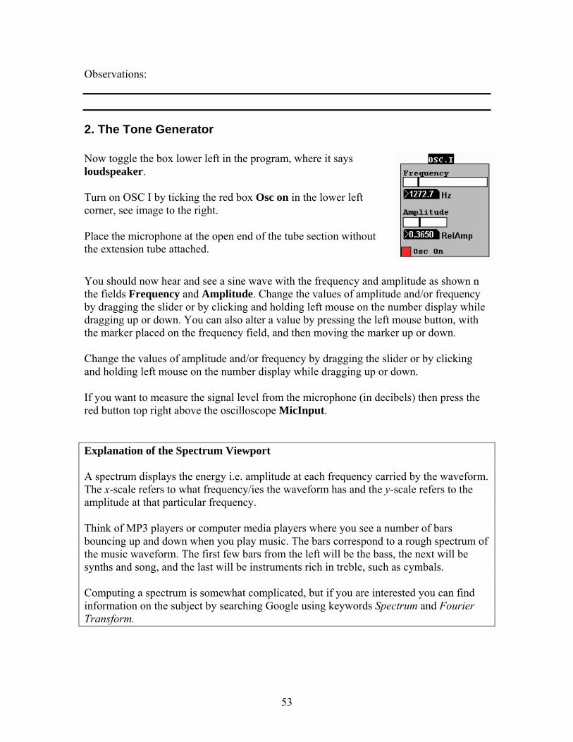
Observations:

2. The Tone Generator Now toggle the box lower left in the program, where it says loudspeaker. Turn on OSC I by ticking the red box Osc on in the lower left corner, see image to the right. Place the microphone at the open end of the tube section without the extension tube attached.

You should now hear and see a sine wave with the frequency and amplitude as shown n the fields Frequency and Amplitude. Change the values of amplitude and/or frequency by dragging the slider or by clicking and holding left mouse on the number display while dragging up or down. You can also alter a value by pressing the left mouse button, with the marker placed on the frequency field, and then moving the marker up or down. Change the values of amplitude and/or frequency by dragging the slider or by clicking and holding left mouse on the number display while dragging up or down. If you want to measure the signal level from the microphone (in decibels) then press the red button top right above the oscilloscope MicInput. Explanation of the Spectrum Viewport A spectrum displays the energy i.e. amplitude at each frequency carried by the waveform. The x-scale refers to what frequency/ies the waveform has and the y-scale refers to the amplitude at that particular frequency. Think of MP3 players or computer media players where you see a number of bars bouncing up and down when you play music. The bars correspond to a rough spectrum of the music waveform. The first few bars from the left will be the bass, the next will be synths and song, and the last will be instruments rich in treble, such as cymbals. Computing a spectrum is somewhat complicated, but if you are interested you can find information on the subject by searching Google using keywords Spectrum and Fourier Transform.

53

3. Microphone Placement Make sure OSC I is active and set the frequency somewhere between 700-1000 Hz. Now place the microphone close to the end of the open tube section, and move it slowly further down the tube. Look at the waveform and spectrum at the same time. How can you see the wave length of sound? Use the measurement scale on the stick attached to the microphone, to measure the wave length of sound, that we call λ (lambda). λ = ___________ [m] Now calculate the speed of sound c with the approximation c = 331,5 + 0,6· T where T is air temperature in degree Celsius c = _________ [m/s]

Calculate the theoretical frequency f by using the formula λcf = .

Theoretical frequency: _____ Hz Frequency set on OSC while measuring: _____ Hz Was there any difference?

4. Resonance Find the resonance frequencies of the tube. The spectrum view is very useful during this task. Type your values in the fields below: Finding the first resonance frequency can be hard, because the small loudspeaker is weak at frequencies below 600 Hz. Tip: increase the amplitude to maximum while scanning lower frequencies only and inspecting the spectrum graph at the same time. First resonance frequency: ______ Hz Second resonance frequency: ______ Hz Third resonance frequency: ______ Hz Calculate the first and second resonance frequencies by using the formula for Open-Closed air column: First resonance frequency: _____ Hz Second resonance frequency: _____ Hz

54

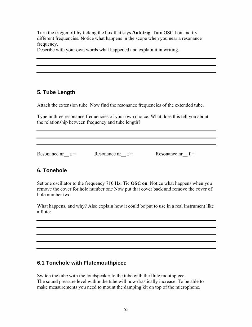
Turn the trigger off by ticking the box that says Autotrig. Turn OSC I on and try different frequencies. Notice what happens in the scope when you near a resonance frequency. Describe with your own words what happened and explain it in writing.

5. Tube Length Attach the extension tube. Now find the resonance frequencies of the extended tube. Type in three resonance frequencies of your own choice. What does this tell you about the relationship between frequency and tube length? Resonance nr__ f = Resonance nr__ f = Resonance nr__ f =

6. Tonehole Set one oscillator to the frequency 710 Hz. Tic OSC on. Notice what happens when you remove the cover for hole number one Now put that cover back and remove the cover of hole number two. What happens, and why? Also explain how it could be put to use in a real instrument like a flute:

6.1 Tonehole with Flutemouthpiece Switch the tube with the loudspeaker to the tube with the flute mouthpiece. The sound pressure level within the tube will now drastically increase. To be able to make measurements you need to mount the damping kit on top of the microphone.

55

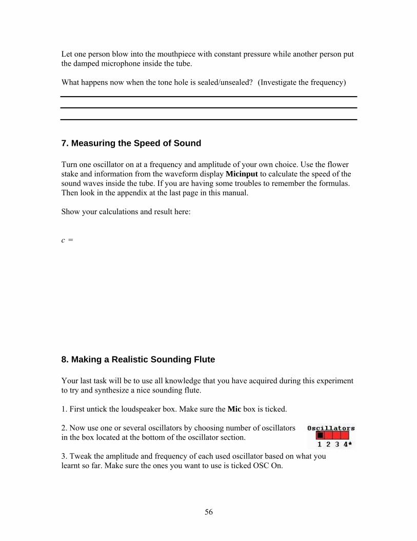
Let one person blow into the mouthpiece with constant pressure while another person put the damped microphone inside the tube. What happens now when the tone hole is sealed/unsealed? (Investigate the frequency)

7. Measuring the Speed of Sound Turn one oscillator on at a frequency and amplitude of your own choice. Use the flower stake and information from the waveform display Micinput to calculate the speed of the sound waves inside the tube. If you are having some troubles to remember the formulas. Then look in the appendix at the last page in this manual. Show your calculations and result here: c =

8. Making a Realistic Sounding Flute Your last task will be to use all knowledge that you have acquired during this experiment to try and synthesize a nice sounding flute. 1. First untick the loudspeaker box. Make sure the Mic box is ticked. 2. Now use one or several oscillators by choosing number of oscillators in the box located at the bottom of the oscillator section. 3. Tweak the amplitude and frequency of each used oscillator based on what you learnt so far. Make sure the ones you want to use is ticked OSC On.

56

4. Then click Flutifier to hear your result. Now continue tweaking until you are satisfied with your result and then play it to the teacher. Tip: Resonance frequencies. If you would like to know more what Flutifier does, ask the teacher!

We hope that the experiment was interesting and fun!

Best wishes from the RealSimPLE team

57

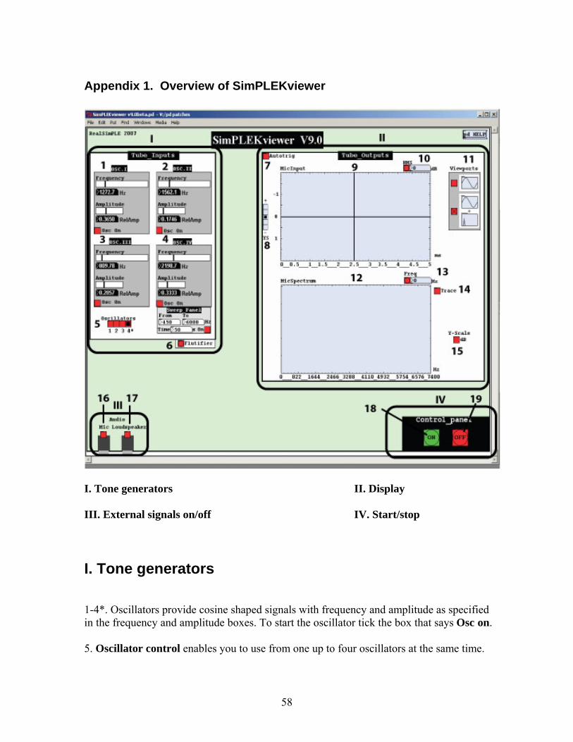
Appendix 1. Overview of SimPLEKviewer

I. Tone generators II. Display III. External signals on/off IV. Start/stop

I. Tone generators

1-4*. Oscillators provide cosine shaped signals with frequency and amplitude as specified in the frequency and amplitude boxes. To start the oscillator tick the box that says Osc on. 5. Oscillator control enables you to use from one up to four oscillators at the same time.

58

6. Flutifier sums all active oscillatorers (active oscillatorers = “osc on”, also make sure loudspeaker on is unticked) signals and adds noise and reverb.

II. Display

7. Autotrig is a trigger function that automatically adjusts the phase so the signal starts from zero on a negative slope (default mode is on). To deactivate it, tick the box. 8. Zoomcontrol enlarges/reduces the waveform. 9. Oscilloscope shows the waveform of the signal fed from the microphone. 10. RMS-value: when clicked the instantaneous amplitude in dB displays. 11. Viewports Viewports makes it possible to switch from single waveform display to waveform display plus spectrum display (default mode is waveform display only) 12. Spectrum shows the spectrum of the signal fed from the microphone. 13. Frequency: when ticked it outputs an estimate of the instantaneous fundamental frequency. 14. Save old values in the spectrum display. If you sweep thru different frequencies you can see all resonant peaks at the same time (default mode is off). 15. Y-scale switches from a linear amplitude scale to a dB scale.

III. External signals on/off

16. Activates the Tube microphone (default is OFF, i.e. no sound is recorded from the tube). For activation tick the box. 17. Activates the Tube speaker (default is OFF, i.e. no sound is fed to the tube). For activation tick the box.

IV. Start/Stop

18. Starts all incoming/outgoing sound and calculations from PD (default is ON).

59

19. Stops all incoming/outgoing sound and calculations from PD: Can also be used for freezing the displays. To start them again press ON.

60

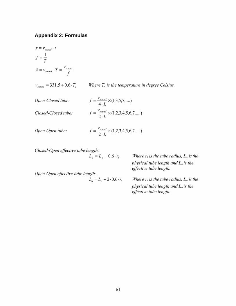
Appendix 2: Formulas

tvx sound ⋅=

Tf 1=

fv

Tv soundsound =⋅=λ

csound Tv ⋅+= 6.05.331 Where Tc is the temperature in degree Celsius.

Open-Closed tube: ,....)7,5,3,1(4

×⋅

=L

vf sound

Closed-Closed tube: .....)7,6,5,4,3,2,1(2

×⋅

=L

vf sound

Open-Open tube: .....)7,6,5,4,3,2,1(2

×⋅

=L

vf sound

Closed-Open effective tube length: tpa rLL ⋅+= 6.0 Where rt is the tube radius, Lp is the

physical tube length and La is the effective tube length.

Open-Open effective tube length: 2 0.6a p tL L= + ⋅ ⋅ r Where r is the tube radius, L ist p the

physical tube length and L

a is the effective tube length.

61