interactive chemistry in the laboratoire de météorologie dynamique
TRANSCRIPT

Atmos. Chem. Phys., 6, 2273–2319, 2006www.atmos-chem-phys.net/6/2273/2006/© Author(s) 2006. This work is licensedunder a Creative Commons License.
AtmosphericChemistry
and Physics
Interactive chemistry in the Laboratoire de MeteorologieDynamique general circulation model: model description andimpact analysis of biogenic hydrocarbons on tropospheric chemistry
G. A. Folberth1,*, D. A. Hauglustaine1, J. Lathi ere1, and F. Brocheton2
1Laboratoire des Sciences du Climat et de l’Environnement (LSCE), Gif-sur-Yvette, France2Centre National de Recherches Meteorologiques (CNRM), Meteo France, Toulouse, France* now at: School of Earth and Ocean Science (SEOS), University of Victoria, Victoria, Canada
Received: 8 July 2005 – Published in Atmos. Chem. Phys. Discuss.: 25 October 2005Revised: 10 February 2006 – Accepted: 28 February 2006 – Published: 21 June 2006
Abstract. We present a description and evaluation of LMDz-INCA, a global three-dimensional chemistry-climate model,pertaining to its recently developed NMHC version. In thissubstantially extended version of the model a comprehensiverepresentation of the photochemistry of non-methane hydro-carbons (NMHC) and volatile organic compounds (VOC)from biogenic, anthropogenic, and biomass-burning sourceshas been included. The tropospheric annual mean methane(9.2 years) and methylchloroform (5.5 years) chemical life-times are well within the range of previous modelling studiesand are in excellent agreement with estimates established bymeans of global observations. The model provides a rea-sonable simulation of the horizontal and vertical distribu-tion and seasonal cycle of CO and key non-methane VOC,such as acetone, methanol, and formaldehyde as comparedto observational data from several ground stations and air-craft campaigns. LMDz-INCA in the NMHC version repro-duces tropospheric ozone concentrations fairly well through-out most of the troposphere. The model is applied in sev-eral sensitivity studies of the biosphere-atmosphere photo-chemical feedback. The impact of surface emissions ofisoprene, acetone, and methanol is studied. These experi-ments show a substantial impact of isoprene on troposphericozone and carbon monoxide concentrations revealing an in-crease in surface O3 and CO levels of up to 30 ppbv and60 ppbv, respectively. Isoprene also appears to significantlyimpact the global OH distribution resulting in a decrease ofthe global mean tropospheric OH concentration by approx-imately 0.7×10⁵ molecules cm−3 or roughly 8% and an in-crease in the global mean tropospheric methane lifetime byapproximately seven months. A global mean ozone net ra-diative forcing due to the isoprene induced increase in the
Correspondence to:G. A. Folberth([email protected])
tropospheric ozone burden of 0.09 W m−2 is found. The keyrole of isoprene photooxidation in the global troposphericredistribution of NOx is demonstrated. LMDz-INCA cal-culates an increase of PAN surface mixing ratios rangingfrom 75 to 750 pptv and 10 to 250 pptv during northernhemispheric summer and winter, respectively. Acetone andmethanol are found to play a significant role in the upper tro-posphere/lower stratosphere (UT/LS) budget of peroxy rad-icals. Calculations with LMDz-INCA show an increase inHOx concentrations region of 8 to 15% and 10 to 15% dueto methanol and acetone biogenic surface emissions, respec-tively. The model has been used to estimate the global tropo-spheric CO budget. A global CO source of 3019 Tg CO yr−1
is estimated. This source divides into a primary source of1533 Tg CO yr−1 and secondary source of 1489 Tg CO yr−1
deriving from VOC photooxidation. Global VOC-to-COconversion efficiencies of 90% for methane and between 20and 45% for individual VOC are calculated by LMDz-INCA.
1 Introduction
Non-Methane volatile organic compounds (NMVOC) areknown to affect the chemical composition of the atmospheredecisively. NMVOC play a key role in the sequestration ofnitrogen oxides (NOx) via the formation of organic nitrates(e.g., PAN and analogs), can directly or indirectly increasethe acidity of precipitation, and provide the starting mate-rial for much of the natural atmospheric aerosols. They havebeen found to significantly contribute to the production ofpollutants and are of major concern in the assessment andcontrolling strategies of present-day and future air quality(e.g.Graedel, 1979; Brasseur and Chatfield, 1991; Crutzenand Zimmermann, 1991; Fehsenfeld et al., 1992; Andreae,
Published by Copernicus GmbH on behalf of the European Geosciences Union.

2274 G. A. Folberth et al.: Biogenic hydrocarbons and tropospheric chemistry
1995; Crutzen, 1995; Andreae and Crutzen, 1997; Berntsenet al., 1997; Levy II et al., 1997; Wang et al., 1998c; Granieret al., 2000; Hauglustaine and Brasseur, 2001). But most im-portant, NMVOC play a central role in tropospheric ozoneformation.
Ozone is a key component in the atmosphere. It is an ef-fective oxidant and greenhouse gas, especially in the uppertroposphere (Lacis et al., 1990; Hauglustaine et al., 1994).In addition, near the surface ozone can have detrimental ef-fects on the vegetation and on human health (Fishman, 1991;Finlaysonpitts and Pitts, 1993; Taylor, 2001; Bernard et al.,2001). Ozone photolysis by ultraviolet radiation is the pri-mary source of hydroxyl radicals in the troposphere. Photo-chemical oxidation of NMVOC, on the other hand, is primar-ily initiated and, hence, controlled by reaction with OH. Thisreaction determines the magnitude and distribution of hy-droxyl radical concentrations, thereby altering the oxidativecapacity of the troposphere (Houweling et al., 1998; Wanget al., 1998c; Poisson et al., 2000).
The direct radiative forcing due to NMVOC has beenfound to be negligibly small. An upper limit to the globalmean anthropogenic forcing of 0.015 W m−2 has been es-tablished byHighwood et al.(1999). Collins et al.(2002),on the other hand, have presented a study, which convinc-ingly demonstrates that NMVOC are able to exert a substan-tial indirect effect on greenhouse warming by affecting ozoneformation and the methane lifetime toward reaction withOH. Moreover, the formation of secondary organic aerosols(SOA) in the course of photochemical NMVOC oxidation isbelieved to have a direct and indirect effect on the radiativeflux of the lower atmosphere (Kanakidou et al., 2000; Tsi-garidis and Kanakidou, 2003).
NMVOC primarily originate from three principle sources:anthropogenic activities, biomass burning, and the biosphere.The biosphere acts as the largest source of reactive tracegases in the troposphere. It has been suggested that the bio-genic source on the global scale surpasses several times thecombined NMVOC emission flux originating from anthro-pogenic and biomass burning sources. State-of-the-art emis-sion estimates include an annual global BVOC source of ap-proximately 750 Tg C yr−1 (Guenther et al., 1995) whereasthe anthropogenic and biomass burning sources togetheramount to roughly 90 Tg C yr−1 of NMVOC (Hao and Liu,1994; Olivier et al., 1996; Olivier and Berdowski, 2001;Olivier et al., 2001; Van der Werf et al., 2003).
Biogenic volatile organic compounds (BVOC) include iso-prene and isoprenoid compounds (such as monoterpenes andhigher terpenes) as well as a large number of other speciesfrom the groups of alkanes, non-isoprenoid alkenes, car-bonyls, alcohols, and organic acids. They are emitted intothe atmosphere from natural sources in terrestrial and marineecosystems. In terms of abundance and importance the pre-dominant BVOC are isoprene and terpenes, methanol, andacetone (Bonsang et al., 1992; MacDonald and Fall, 1993;Sharkey and Singsaas, 1995; Kirstine et al., 1998; Bonsang
and Boissard, 1999; Doskey and Gao, 1999; Guenther et al.,2000; Singh et al., 2000; Galbally and Kirstine, 2002; Jacobet al., 2002).
An increasing importance of isoprene (Shallcross andMonks, 2000; Sanderson et al., 2003) and other BVOC(Guenther et al., 1999; Kellomaki et al., 2001; Lathiere et al.,2005a; Hauglustaine et al., 2005) in the future has been hy-pothesized due to an increasing net primary production as-sociated with a warmer climate (Constable et al., 1999). Ifglobal patterns and magnitudes of biogenic VOC emissionschange in correlation with climate-related alterations in tem-perature, precipitation, and solar insolation, in turn a feedback upon the climate via changes in the accumulation rateof atmospheric greenhouse gases seems very likely.
Hauglustaine et al.(2004) recently presented the globalclimate-chemistry model LMDz-INCA, which takes into ac-count the CH4–NOx–CO–O3 chemistry of the backgroundtroposphere. This model has been supplemented by a de-tailed non-methane hydrocarbon scheme in order to inves-tigate biosphere-atmosphere interactions. This work repre-sents a further step in the framework of several ongoing stud-ies (Boucher et al., 2002; Hauglustaine et al., 2004; Baueret al., 2004), which eventually will converge toward a mod-elling system that takes into account the “complete” chem-istry of the troposphere and stratosphere, including the dif-ferent types of aerosols, in a fully interactive Earth SystemModel.
In this work we present the non-methane hydrocarbon ver-sion of INCA (version NMHC.1.0). A description and gen-eral evaluation of this new model version is provided. Themore general application abilities are than used to investi-gate various aspects of biosphere NMVOC emissions andtropospheric chemical composition including ozone forma-tion, tropospheric HOx, and possible impacts on future cli-mate.
2 Model description
2.1 The LMDz General Circulation Model
LMDz (Laboratoire deM eteorologieDynamique,zoom) isa grid point General Circulation Model (GCM) developedinitially for climate studies bySadourny and Laval(1984).As part of the IPSL Earth System Model, the GCM lately hasundergone a major recoding and has been applied in climatefeedback studies byFriedlingstein et al.(2001) andDufresneet al.(2002).
In LMDz the finite volume transport scheme ofVan Leer(1977) as described inHourdin and Armengaud(1999) isused to calculate large-scale advection of tracers. The pa-rameterization of deep convection is based on the schemeof Tiedtke(1989); a local second-order closure formalism isused to describe turbulent mixing in the planetary boundarylayer (PBL).
Atmos. Chem. Phys., 6, 2273–2319, 2006 www.atmos-chem-phys.net/6/2273/2006/
G. A. Folberth et al.: Biogenic hydrocarbons and tropospheric chemistry 2275
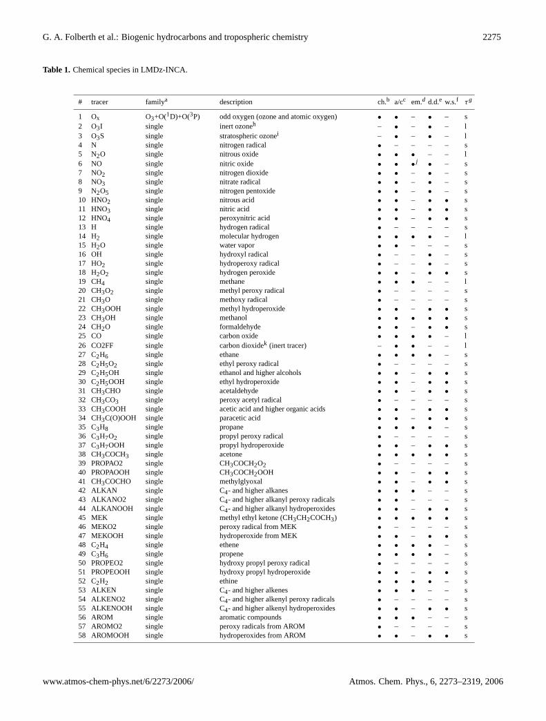
Table 1. Chemical species in LMDz-INCA.
# tracer familya description ch.b a/cc em.d d.d.e w.s.f τg
1 Ox O3+O(1D)+O(3P) odd oxygen (ozone and atomic oxygen) • • – • – s2 O3I single inert ozoneh – • – • – l3 O3S single stratospheric ozonei – • – • – l4 N single nitrogen radical • – – – – s5 N2O single nitrous oxide • • • – – l6 NO single nitric oxide • • •
j• – s
7 NO2 single nitrogen dioxide • • – • – s8 NO3 single nitrate radical • • – • – s9 N2O5 single nitrogen pentoxide • • – • – s10 HNO2 single nitrous acid • • – • • s11 HNO3 single nitric acid • • – • • s12 HNO4 single peroxynitric acid • • – • • s13 H single hydrogen radical • – – – – s14 H2 single molecular hydrogen • • • • – l15 H2O single water vapor • • – – – s16 OH single hydroxyl radical • – – • – s17 HO2 single hydroperoxy radical • – – • – s18 H2O2 single hydrogen peroxide • • – • • s19 CH4 single methane • • • – – l20 CH3O2 single methyl peroxy radical • – – – – s21 CH3O single methoxy radical • – – – – s22 CH3OOH single methyl hydroperoxide • • – • • s23 CH3OH single methanol • • • • • s24 CH2O single formaldehyde • • – • • s25 CO single carbon oxide • • • • – l26 CO2FF single carbon dioxidek (inert tracer) – • • – – l27 C2H6 single ethane • • • • – s28 C2H5O2 single ethyl peroxy radical • – – – – s29 C2H5OH single ethanol and higher alcohols • • – • • s30 C2H5OOH single ethyl hydroperoxide • • – • • s31 CH3CHO single acetaldehyde • • – • • s32 CH3CO3 single peroxy acetyl radical • – – – – s33 CH3COOH single acetic acid and higher organic acids • • – • • s34 CH3C(O)OOH single paracetic acid • • – • • s35 C3H8 single propane • • • • – s36 C3H7O2 single propyl peroxy radical • – – – – s37 C3H7OOH single propyl hydroperoxide • • – • • s38 CH3COCH3 single acetone • • • • • s39 PROPAO2 single CH3COCH2O2 • – – – – s40 PROPAOOH single CH3COCH2OOH • • – • • s41 CH3COCHO single methylglyoxal • • – • • s42 ALKAN single C4- and higher alkanes • • • – – s43 ALKANO2 single C4- and higher alkanyl peroxy radicals • • – – – s44 ALKANOOH single C4- and higher alkanyl hydroperoxides • • – • • s45 MEK single methyl ethyl ketone (CH3CH2COCH3) • • • • • s46 MEKO2 single peroxy radical from MEK • – – – – s47 MEKOOH single hydroperoxide from MEK • • – • • s48 C2H4 single ethene • • • • – s49 C3H6 single propene • • • • – s50 PROPEO2 single hydroxy propyl peroxy radical • – – – – s51 PROPEOOH single hydroxy propyl hydroperoxide • • – • • s52 C2H2 single ethine • • • • – s53 ALKEN single C4- and higher alkenes • • • – – s54 ALKENO2 single C4- and higher alkenyl peroxy radicals • – – – – s55 ALKENOOH single C4- and higher alkenyl hydroperoxides • • – • • s56 AROM single aromatic compounds • • • – – s57 AROMO2 single peroxy radicals from AROM • – – – – s58 AROMOOH single hydroperoxides from AROM • • – • • s
www.atmos-chem-phys.net/6/2273/2006/ Atmos. Chem. Phys., 6, 2273–2319, 2006
2276 G. A. Folberth et al.: Biogenic hydrocarbons and tropospheric chemistry
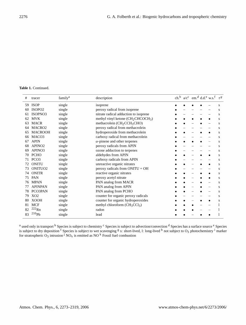
Table 1. Continued.
# tracer familya description ch.b a/cc em.d d.d.e w.s.f τg
59 ISOP single isoprene • • • • – s60 ISOPO2 single peroxy radical from isoprene • – – – – s61 ISOPNO3 single nitrate radical adduction to isoprene • – – – – s62 MVK single methyl vinyl ketone (CH2CHCOCH3) • • • • • s63 MACR single methacrolein (CH2CCH3CHO) • • – • – s64 MACRO2 single peroxy radical from methacrolein • – – – – s65 MACROOH single hydroperoxide from methacrolein • • – • • s66 MACO3 single carboxy radical from methacrolein • – – – – s67 APIN single α-pinene and other terpenes • • • • – s68 APINO2 single peroxy radicals from APIN • – – – – s69 APINO3 single ozone adduction to terpenes • – – – – s70 PCHO single aldehydes from APIN • • – • • s71 PCO3 single carboxy radicals from APIN • – – – – s72 ONITU single unreactive organic nitrates • • – • • s73 ONITUO2 single peroxy radicals from ONITU + OH • – – – – s74 ONITR single reactive organic nitrates • • – • • s75 PAN single peroxy acetyl nitrate • • – • • s76 MPAN single PAN analog from MACR • • – • – s77 APINPAN single PAN analog from APIN • • – • – s78 PCO3PAN single PAN analog from PCHO • • – • – s79 XO2 single counter for organic peroxy radicals • – – – – s80 XOOH single counter for organic hydroperoxides • • – • • s81 MCF single methyl chloroform (CH3CCl3) • • • – – l82 222Rn single radon • • • – – l83 210Pb single lead • • – • • l
a used only in transportb Species is subject to chemistryc Species is subject to advection/convectiond Species has a surface sourcee Speciesis subject to dry depositionf Species is subject to wet scavengingg s: short-lived, l: long-livedh not subject to O3 photochemistryi markerfor stratospheric O3 intrusionj NOx is emitted as NOk Fossil fuel combustion
Atmos. Chem. Phys., 6, 2273–2319, 2006 www.atmos-chem-phys.net/6/2273/2006/
G. A. Folberth et al.: Biogenic hydrocarbons and tropospheric chemistry 2277
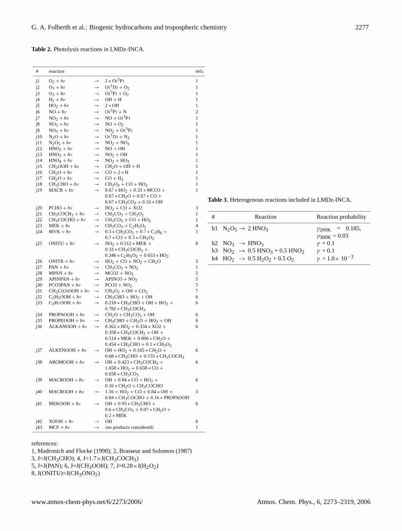
Table 2. Photolysis reactions in LMDz-INCA.
# reaction refs.
j1 O2 + hν → 2 ∗ O(3P) 1j2 O3 + hν → O(1D) + O2 1j3 O3 + hν → O(3P) + O2 1j4 H2 + hν → OH + H 1j5 HO2 + hν → 2 ∗ OH 1j6 NO + hν → O(3P) + N 2j7 NO2 + hν → NO + O(3P) 1j8 NO3 + hν → NO + O2 1j9 NO3 + hν → NO2 + O(3P) 1j10 N2O + hν → O(1D) + N2 1j11 N2O5 + hν → NO2 + NO3 1j12 HNO2 + hν → NO + OH 1j13 HNO3 + hν → NO2 + OH 1j14 HNO4 + hν → NO2 + HO2 1j15 CH3OOH+ hν → CH2O + OH + H 1j16 CH2O + hν → CO+ 2 ∗ H 1j17 CH2O + hν → CO+ H2 1j18 CH3CHO+ hν → CH3O2 + CO+ HO2 1j19 MACR + hν → 0.67∗ HO2 + 0.33∗ MCO3+
0.67∗ CH2O + 0.67∗ CO+
0.67∗ CH3CO3 + 0.33∗ OH
1
j20 PCHO+ hν → HO2 + CO+ XO2 3j21 CH3COCH3 + hν → CH3CO3 + CH3O2 1j22 CH3COCHO+ hν → CH3CO3 + CO+ HO2 1j23 MEK + hν → CH3CO3 + C2H5O2 4j24 MVK + hν → 0.3 ∗ CH3CO3 + 0.7 ∗ C3H6 +
0.7 ∗ CO+ 0.3 ∗ CH3O2
1
j25 ONITU + hν → NO2 + 0.512∗ MEK +
0.33∗ CH3COCH3 +
0.346∗ C2H5O2 + 0.653∗ HO2
8
j26 ONITR+ hν → HO2 + CO+ NO2 + CH2O 3j27 PAN+ hν → CH3CO3 + NO2 1j28 MPAN + hν → MCO2+ NO2 5j29 APINPAN+ hν → APINO3+ NO2 5j30 PCO3PAN+ hν → PCO3+ NO2 5j31 CH3C(O)OOH+ hν → CH3O2 + OH + CO2 7j32 C2H5OOH+ hν → CH3CHO+ HO2 + OH 6j33 C3H7OOH+ hν → 0.218∗ CH3CHO+ OH + HO2 +
0.782∗ CH3COCH3
6
j34 PROPAOOH+ hν → CH2O + CH3CO3 + OH 6j35 PROPEOOH+ hν → CH3CHO+ CH2O + HO2 + OH 6j36 ALKANOOH + hν → 0.562∗ HO2 + 0.334∗ XO2 +
0.358∗ CH3COCH2 + OH +
0.514∗ MEK + 0.006∗ CH2O +
0.454∗ CH3CHO+ 0.1 ∗ CH3O2
6
j37 ALKENOOH + hν → OH + HO2 + 0.165∗ CH2O +
0.68∗ CH3CHO+ 0.155∗ CH3COCH3
6
j38 AROMOOH+ hν → OH + 0.423∗ CH3COCH3 +
1.658∗ HO2 + 0.658∗ CO+
0.658∗ CH3CO3
6
j39 MACROOH+ hν → OH + 0.84∗ CO+ HO2 +
0.16∗ CH2O + CH3COCHO6
j40 MACROOH+ hν → 1.16+ HO2 + CO+ 0.84∗ OH +
0.84∗ CH3COCHO+ 0.16∗ PROPAOOH3
j41 MEKOOH+ hν → OH + 0.93∗ CH3CHO+
0.6 ∗ CH3CO3 + 0.07∗ CH2O +
0.2 ∗ MEK
6
j42 XOOH+ hν → OH 6j43 MCF+ hν → (no products considered) 1
references:1, Madronich and Flocke(1998); 2, Brasseur and Solomon(1987)3, J=J(CH3CHO); 4, J=1.7×J(CH3COCH3)5, J=J(PAN); 6, J=J(CH3OOH); 7, J=0.28×J(H2O2)8, J(ONITU)=J(CH3ONO2)
Table 3. Heterogenous reactions included in LMDz-INCA.
# Reaction Reaction probability
h1 N2O5 → 2 HNO3 γ200K = 0.185,γ300K = 0.03
h2 NO3 → HNO3 γ = 0.1h3 NO2 → 0.5 HNO3 + 0.5 HNO2 γ = 0.1h4 HO2 → 0.5 H2O2 + 0.5 O2 γ = 1.0× 10⁻³
www.atmos-chem-phys.net/6/2273/2006/ Atmos. Chem. Phys., 6, 2273–2319, 2006

2278 G. A. Folberth et al.: Biogenic hydrocarbons and tropospheric chemistry
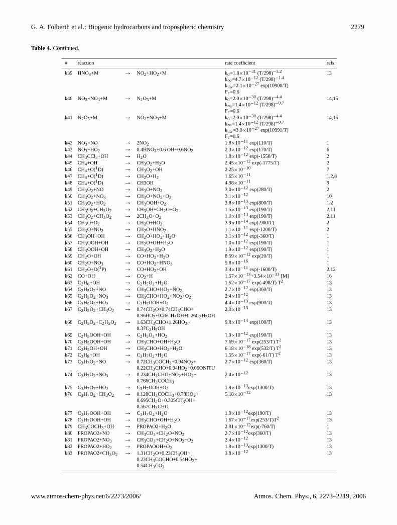
Table 4. Thermochemical reactions in LMDz-INCA.
# reaction rate coefficient refs.
k1 O(3P)+O2+M → O3+M 6.0×10⁻³⁴ (300/T)2.3 2k2 O(3P)+O(3P)+M → O2+M 4.23×10⁻²⁸ T−2.0 14,15k3 O(3P)+O3 → 2 O2 8.0×10⁻¹² exp(-2060/T) 1k4 O(1D)+O3 → 2 O2 1.2×10⁻¹⁰ 2k5 O(1D)+N2 → O(3P)+N2 1.8×10⁻¹¹ exp(107/T) 1k6 O(1D)+O2 → O(3P)+O2 3.2×10⁻¹¹ exp(67/T) 1k7 O(1D)+H2O → 2 OH 2.2×10⁻¹⁰ 2k8 O(1D)+H2 → OH+H 1.1×10⁻¹⁰ 1,2k9 O(1D)+N2O → 2 NO 6.7×10⁻¹¹ 2k10 O(1D)+N2O → N2+O2 4.4×10⁻¹¹ 1k11 O2+N → NO+O(3P) 1.5×10⁻¹¹ exp(-3600/T) 2k12 O2+H+M → HO2+M k0=5.69×10⁻³² (T/298)−1.6
k∞=7.5×10⁻¹¹
Fc=0.6
2
k13 O3+H → OH+O2 1.0×10⁻¹⁰ exp(-367/T) 5k14 OH+O(3P) → H+O2 2.2×10⁻¹¹ exp(120/T) 2k15 OH+O3 → HO2+O2 1.9×10⁻¹² exp(-1000/T) 1k16 OH+H2 → H2O+H 5.5×10⁻¹² exp(-2000/T) 2k17 OH+OH → H2O+O(3P) 4.2×10⁻¹² exp(-240/T) 2k18 OH+HO2 → H2O+O2 4.8×10⁻¹¹ exp(250/T) 1,2k19 OH+H2O2 → H2O+HO2 2.9×10⁻¹² exp(-160/T) 1,2k20 OH+HNO2 → H2O+NO2 1.8×10⁻¹¹ exp(-390/T) 2k21 OH+HNO3 → H2O+NO3 k1=7.2×10⁻¹⁵ exp(785/T)
k2=4.1×10⁻¹⁶ exp(1440/T)k3=1.9×10−33 exp(725/T) [M]
k = k1 +k3
1 +k3k2
13
k22 OH+HNO4 → H2O+NO2+O2 1.3×10⁻¹² exp(380/T) 2k23 HO2+O(3P) → OH+O2 3.0×10⁻¹¹ exp(200/T) 2k24 HO2+O3 → OH+2 O2 1.1×10⁻¹⁴ exp(-500/T) 2k25 HO2+H → 2 OH 7.2×10⁻¹¹ 1k26 HO2+H → H2+O2 5.6×10⁻¹² 1k27 HO2+H → H2O+O(3P) 2.4×10⁻¹² 1k28 HO2+HO2 → H2O2+O2 k0=2.3×10⁻¹³ (600/T)
k∞=1.7×10⁻³³ [M] exp(1000/T)Fc=1.0+1.4×10−21 [H2O] exp(2200/T)
k = (k0 + k∞) Fc
14,15
k29 NO+O3 → NO2+O2 1.8×10⁻¹² exp(-1370/T) 1k30 NO+OH+M → HNO2+M k0=7.01×10⁻³¹ (T/298)−2.6
k∞=3.6×10⁻¹¹ (T/298)−0.1
Fc=0.6
2
k31 NO+HO2 → NO2+OH 3.5×10⁻¹² exp(250/T) 2k32 NO+N → N2+O(3P) 2.1×10⁻¹¹ exp(100/T) 2k33 NO2+O(3P) → NO+O2 6.5×10⁻¹² exp(120/T) 1,2k34 NO2+O(3P)+M → NO3+M k0=9.0×10⁻³² (T/298)−2.0
k∞=2.2×10⁻¹¹
Fc=0.6
2
k35 NO2+O3 → NO3+O2 1.2×10⁻¹³ exp(-2450/T) 2k36 NO2+H → OH+NO 4.0×10⁻¹⁰ exp(-340/T) 2k37 NO2+OH+M → HNO3+M k0=2.6×10⁻³⁰ (T/298)−2.9
k∞=7.5×10⁻¹¹ (T/298)−0.6
Fc=0.6
1
k38 NO2+HO2+M → HNO4+M k0=1.8×10⁻³¹ (T/298)−3.2
k∞=4.7×10⁻¹² (T/298)−1.4
Fc=0.6
13
Atmos. Chem. Phys., 6, 2273–2319, 2006 www.atmos-chem-phys.net/6/2273/2006/
G. A. Folberth et al.: Biogenic hydrocarbons and tropospheric chemistry 2279
Table 4. Continued.
# reaction rate coefficient refs.
k39 HNO4+M → NO2+HO2+M k0=1.8×10⁻³¹ (T/298)−3.2
k∞=4.7×10⁻¹² (T/298)−1.4
kinv=2.1×10⁻²⁷ exp(10900/T)Fc=0.6
13
k40 NO2+NO3+M → N2O5+M k0=2.0×10⁻³⁰ (T/298)−4.4
k∞=1.4×10⁻¹² (T/298)−0.7
Fc=0.6
14,15
k41 N2O5+M → NO2+NO3+M k0=2.0×10⁻³⁰ (T/298)−4.4
k∞=1.4×10⁻¹² (T/298)−0.7
kinv=3.0×10⁻²⁷ exp(10991/T)Fc=0.6
14,15
k42 NO3+NO → 2NO2 1.8×10⁻¹¹ exp(110/T) 1k43 NO3+HO2 → 0.4HNO3+0.6 OH+0.6NO2 2.3×10⁻¹² exp(170/T) 6k44 CH3CCl3+OH → H2O 1.8×10⁻¹² exp(-1550/T) 2k45 CH4+OH → CH3O2+H2O 2.45×10⁻¹² exp(-1775/T) 2k46 CH4+O(1D) → CH3O2+OH 2.25×10⁻¹⁰ 7k47 CH4+O(1D) → CH2O+H2 1.65×10⁻¹¹ 1,2,8k48 CH4+O(1D) → CH3OH 4.98×10⁻¹¹ 9k49 CH3O2+NO → CH3O+NO2 3.0×10⁻¹² exp(280/T) 2k50 CH3O2+NO3 → CH3O+NO2+O2 3.1×10⁻¹² 10k51 CH3O2+HO2 → CH3OOH+O2 3.8×10⁻¹³ exp(800/T) 1,2k52 CH3O2+CH3O2 → CH3OH+CH2O+O2 1.5×10⁻¹³ exp(190/T) 2,11k53 CH3O2+CH3O2 → 2CH3O+O2 1.0×10⁻¹³ exp(190/T) 2,11k54 CH3O+O2 → CH2O+HO2 3.9×10⁻¹⁴ exp(-900/T) 2k55 CH3O+NO2 → CH2O+HNO2 1.1×10⁻¹¹ exp(-1200/T) 2k56 CH3OH+OH → CH2O+HO2+H2O 3.1×10⁻¹² exp(-360/T) 1k57 CH3OOH+OH → CH2O+OH+H2O 1.0×10⁻¹² exp(190/T) 1k58 CH3OOH+OH → CH3O2+H2O 1.9×10⁻¹² exp(190/T) 1k59 CH2O+OH → CO+HO2+H2O 8.59×10⁻¹² exp(20/T) 1k60 CH2O+NO3 → CO+HO2+HNO3 5.8×10⁻¹⁶ 1k61 CH2O+O(3P) → CO+HO2+OH 3.4×10⁻¹¹ exp(-1600/T) 2,12k62 CO+OH → CO2+H 1.57×10⁻¹³+3.54×10⁻³³ [M] 16k63 C2H6+OH → C2H5O2+H2O 1.52×10⁻¹⁷ exp(-498/T) T2 13k64 C2H5O2+NO → CH3CHO+HO2+NO2 2.7×10⁻¹² exp(360/T) 13k65 C2H5O2+NO3 → CH3CHO+HO2+NO2+O2 2.4×10⁻¹² 13k66 C2H5O2+HO2 → C2H5OOH+O2 4.4×10⁻¹³ exp(900/T) 13k67 C2H5O2+CH3O2 → 0.74CH2O+0.74CH3CHO+
0.96HO2+0.26CH3OH+0.26C2H5OH2.0×10−13 13
k68 C2H5O2+C2H5O2 → 1.63CH3CHO+1.26HO2+0.37C2H5OH
9.8×10⁻¹⁴ exp(100/T) 13
k69 C2H5OOH+OH → C2H5O2+HO2 1.9×10⁻¹² exp(190/T) 13k70 C2H5OOH+OH → CH3CHO+OH+H2O 7.69×10⁻¹⁷ exp(253/T) T2 13k71 C2H5OH+OH → CH3CHO+HO2+H2O 6.18×10⁻¹⁸ exp(532/T) T2 13k72 C3H8+OH → C3H7O2+H2O 1.55×10⁻¹⁷ exp(-61/T) T2 13k73 C3H7O2+NO → 0.72CH3COCH3+0.94NO2+
0.22CH3CHO+0.94HO2+0.06ONITU2.7×10−12 exp(360/T) 13
k74 C3H7O2+NO3 → 0.234CH3CHO+NO2+HO2+0.766CH3COCH3
2.4×10⁻¹² 13
k75 C3H7O2+HO2 → C3H7OOH+O2 1.9×10⁻¹³exp(1300/T) 13k76 C3H7O2+CH3O2 → 0.128CH3COCH3+0.78HO2+
0.695CH2O+0.305CH3OH+0.567CH3CHO
5.18×10⁻¹² 13
k77 C3H7OOH+OH → C3H7O2+H2O 1.9×10⁻¹²exp(190/T) 13k78 C3H7OOH+OH → CH3CHO+OH+H2O 1.67×10⁻¹⁷exp(253/T)T2 13k79 CH3COCH3+OH → PROPAO2+H2O 2.81×10⁻¹²exp(-760/T) 1k80 PROPAO2+NO → CH3CO3+CH2O+NO2 2.7×10⁻¹²exp(360/T) 13k81 PROPAO2+NO3 → CH3CO3+CH2O+NO2+O2 2.4×10⁻¹² 13k82 PROPAO2+HO2 → PROPAOOH+O2 1.9×10⁻¹³exp(1300/T) 13k83 PROPAO2+CH3O2 → 1.31CH2O+0.23CH3OH+
0.23CH3COCHO+0.54HO2+0.54CH3CO3
3.8×10⁻¹² 13
www.atmos-chem-phys.net/6/2273/2006/ Atmos. Chem. Phys., 6, 2273–2319, 2006

2280 G. A. Folberth et al.: Biogenic hydrocarbons and tropospheric chemistry
Table 4. Continued.
# reaction rate coefficient refs.
k84 PROPAOOH+OH → PROPAO2+H2O 1.9×10⁻¹²exp(190/T) 13k85 PROPAOOH+OH → CH3COCHO+OH+H2O 4.69×10⁻¹⁷exp(253/T)T2 13k86 C2H4+OH+M → 0.667PROPEO2+M k0=1.0×10⁻²⁸(T/298)−0.8
k∞=8.79×10⁻¹²
Fc=0.7
2
k87 C2H4+O3 → CH2O+0.46CO+0.16HO2+0.08OH+0.17CO2
1.2×10⁻¹⁴exp(-2630/T) 2
k88 C3H6+OH+M → PROPEO2+M k0=2.94×10⁻²⁷(T/298)−3.0
k∞=2.775×10⁻¹¹(T/298)−1.3
Fc=0.5
13
k89 C3H6+O3 → 0.63248CH2O+0.341CH3O2+0.0868CH4+0.4166CO+0.0124CH3OH+0.2096HO2+0.2474OH+0.38CH3CHO+0.2754CO2
6.51×10⁻¹⁵exp(-1900/T) 2
k90 PROPEO2+NO → CH3CHO+CH2O+HO2+NO2 2.7×10⁻¹²exp(360/T) 13k91 PROPEO2+NO3 → CH3CHO+CH2O+ HO2+NO2+O2 2.4×10⁻¹² 13k92 PROPEO2+HO2 → PROPEOOH+O2 1.9×10⁻¹³exp(1300/T) 13k93 PROPEO2+CH3O2 → 0.305CH3OH+0.78HO2+
1.085CH2O+0.39CH3CHO+0.305CH3COCHO
7.583×10⁻¹³ 13
k94 PROPEOOH+OH → PROPEO2+H2O 1.9×10⁻¹²exp(190/T) 13k95 PROPEOOH+OH → CH3COCHO+OH+H2O 2.35×10⁻¹⁷exp(696/T)T2 13k96 PROPEOOH+OH → CH3COCHO+OH+H2O 2.69×10⁻¹⁷exp(253/T)T2 13k97 PROPEOOH+OH → CH3CHO+HO2+H2O 1.26×10⁻¹⁷exp(253/T)T2 13k98 PROPEOOH+OH → PROPAOOH+HO2+H2O 3.19×10⁻¹⁸exp(696/T)T2 13k99 CH3CHO+OH → CH3CO3+H2O 5.6×10⁻¹²exp(270/T) 2k100 CH3CHO+NO3 → CH3CO3+HNO3 1.4×10⁻¹²exp(-1860/T) 13k101 CH3CO3+NO → CH3O2+NO2+CO2 5.3×10⁻¹²exp(360/T) 13k102 CH3CO3+NO2+M → PAN+M k0=2.7×10⁻²⁸(T/298)−7.1
k∞=1.2×10⁻¹¹(T/298)−0.9
Fc=0.3
13
k103 PAN+M → CH3CO3+NO2+M k0=5.0×10⁻²exp(-12875/T)k∞=2.2×10+16exp(-13435/T)Fc=0.27
13
k104 CH3CO3+NO3 → CH3O2+NO2+CO2+O2 5.0×10⁻¹² 13k105 CH3CO3+HO2 → 0.3O3+0.3CH3OOH+
0.7O2+0.7CH3C(O)OOH4.3×10−13exp(1040/T) 13
k106 CH3CO3+CH3O2 → CH2O+0.86CH3O2+0.86HO2+0.86CO2+O2+0.14CH3COOH
1.3×10⁻¹²exp(640/T) 13
k107 CH3CO3+CH3CO3 → 2CH3O2+2CO2 2.3×10⁻¹²exp(530/T) 13k108 CH3C(O)OOH+OH → CH3CO3+H2O 1.9×10⁻¹²exp(190/T) 13k109 C2H2+OH+M → 0.36CO+0.64CH3COCHO+
0.36HO2+0.65OH+Mk0=5.01×10⁻³⁰(T/298)−1.5
k∞=9.0×10⁻¹³(T/298)2.0
Fc=0.62
1
k110 ISOP+OH → ISOPO2 2.89×10⁻¹¹exp(335/T) 1,2k111 ISOP+O3 → 0.42MACR+0.16MVK+
0.05C3H6+0.18OH+0.09HO2+0.42CH2O+0.27CO+0.07H2+0.15CO2
9.36×10⁻¹⁵exp(-1913/T) 13
k112 ISOP+NO3 → ISOPNO3 3.03×10⁻¹²exp(-446/T) 13k113 ISOPO2+NO → 0.12ONITR+0.88NO2+
0.76HO2+0.608CH2O+0.404MACR+0.354MVK+0.12XO2
2.7×10⁻¹²exp(360/T) 13
k114 ISOPO2+NO3 → 0.864HO2+NO2+0.69CH2O+0.46MACR+0.403MVK+0.136XO2
2.4×10⁻¹² 13
k115 ISOPO2+HO2 → 0.867HO2+0.739CH2O+0.506MACR+0.429MVK+0.133XO2+XOOH
1.9×10⁻¹³exp(1300/T) 13
Atmos. Chem. Phys., 6, 2273–2319, 2006 www.atmos-chem-phys.net/6/2273/2006/

G. A. Folberth et al.: Biogenic hydrocarbons and tropospheric chemistry 2281
Table 4. Continued.
# reaction rate coefficient refs.
k116 ISOPO2+CH3O2 → 0.305CH3OH+0.703HO2+0.91CH2O+0.137XO2+0.351MACR+0.205MVK
1.33×10⁻¹² 13
k117 ISOPO2+CH3CO3 → 0.275CH3COOH+0.58HO2+0.725CO+0.725CH3O2+0.198XO+20.397CH2O+0.504MACR+0.296MVK
7.96×10⁻¹² 13
k118 ISOPNO3+NO → 1.206NO2+0.794HO2+0.072CH2O+0.167MACR+0.039MVK+0.794ONITR
2.7×10⁻¹²exp(360/T) 13
k119 ISOPNO3+NO3 → 1.206NO2+0.794HO2+0.072CH2O+0.167MACR+0.039MVK+0.794ONITR
2.4×10⁻¹² 13
k120 ISOPNO3+HO2 → 0.206NO2+0.794HO2+0.008CH2O+0.167MACR+0.039MVK+0.794ONITR+XOOH
1.9×10⁻¹³exp(1300/T) 13
k121 ISOPNO3+CH3O2 → 0.305CH3OH+0.711HO2+0.697CH2O+0.06NO2+0.059MACR+0.001MVK+0.635ONITR
1.749×10⁻¹² 13
k122 APIN+OH → APINO2 1.08×10⁻¹¹exp(444/T) 13k123 APIN+O3 → 0.56OH+0.56APINO3 1.1615×10⁻¹⁵exp(-732/T) 13k124 APIN+NO3 → APINO2+NO2 1.19×10⁻¹²exp(490/T) 13k125 APINO2+NO → PCHO+NO2+HO2 2.7×10⁻¹²exp(360/T) 13k126 APINO2+NO3 → PCHO+NO2+HO2+O2 2.4×10⁻¹² 13k127 APINO2+HO2 → PCHO+HO2+XOOH 1.9×10⁻¹³exp(1300/T) 13k128 APINO2+CH3O2 → 0.305CH3OH+0.695APINO3+HO2 1.22×10⁻¹³ 13k129 APINO2+CH3CO3 → 0.725CO2+0.725CH3O2+
0.725PCHO+0.725HO2+0.275CH3COOH
7.37×10⁻¹³ 13
k130 APINO3+NO → NO2+CO2+CH3COCH3+ 2PROPEO2 5.3×10⁻¹²exp(360/T) 13k131 APINO3+NO2+M → APINPAN+M k0=2.7×10⁻²⁸(T/298)−7.1
k∞=1.2×10⁻¹¹(T/298)−0.9
Fc=0.3
13
k132 APINPAN+M → APINO3+NO2+M k0=4.0×10⁻³exp(-12100/T)k∞=5.4×10+16exp(-13830/T)Fc=0.3
14,15
k133 APINO3+NO3 → NO2+CO2+CH3COCH3+2PROPEO2+O2
5.0×10⁻¹² 13
k134 APINO3+HO2 → 0.3O3+0.3CH3COOH+0.7O2+0.7CH3C(O)OOH
4.3×10⁻¹³exp(1040/T) 13
k135 APINO3+CH3O2 → 0.335CH2O+0.665CH2O+0.665HO2+0.665CH3COCH3+1.33PROPEO2+CO2
4.52×10⁻¹² 13
k136 APINO3+CH3CO3 → 2CO2+CH3O2+CH3COCH3+2PROPEO2
4.6×10⁻¹²exp(530/T) 13
k137 APINO3+APINO3 → 2CO2+2CH3COCH3+4PROPEO2 2.3×10⁻¹²exp(530/T) 13k138 MACR+OH → 0.5MACRO2+0.5HO2+0.5MCO3 1.86×10⁻¹¹exp(175/T) 13k139 MACR+O3 → 0.8CH3COCHO+0.13HO2+
0.37CO+0.1H2+0.2OH+0.34CH2O+0.14CO2
1.359×10⁻¹⁵exp(-2112/T) 13
k140 MVK+OH → MACRO2 2.67×10⁻¹²exp(452/T) 13k141 MVK+O3 → 0.05CH2O+0.95CH3COCHO+
0.08OH+0.15HO2+0.12H2+0.16CO2+0.44CO
7.51×10⁻¹⁶exp(-1521/T) 13
k142 MACRO2+NO → 0.015ONITR+0.985NO2+0.985HO2+0.158CH2O+0.158CH3COCHO+0.828CO+0.828CH3COCHO
2.7×10⁻¹²exp(360/T) 13
www.atmos-chem-phys.net/6/2273/2006/ Atmos. Chem. Phys., 6, 2273–2319, 2006
2282 G. A. Folberth et al.: Biogenic hydrocarbons and tropospheric chemistry
Table 4. Continued.
# reaction rate coefficient refs.
k143 MACRO2+NO3 → NO2+HO2+0.16CH2O+0.16CH3COCHO+0.84CO+0.84CH3COCHO
2.4×10⁻¹² 13
k144 MACRO2+HO2 → MACROOH 1.9×10⁻¹³exp(1300/T) 13k145 MACRO2+CH3O2 → 0.916HO2+1.064CH2O+
0.458CO+0.458CH3COCHO+0.229CH3OH+0.458CH3CHO+
4.1288×10⁻¹³ 13
k146 MACRO2+CH3CO3 → 0.794CO2+0.794CH3O2+0.412CH3CHO+0.544CH2O+0.794CH3COCHO+0.794HO2+0.206CH3COOH+0.25CO
2.475×10⁻¹² 13
k147 MACROOH+OH → MACRO2+H2O 1.9×10⁻¹²exp(190/T) 13k148 MACROOH+OH → 2CH3CHO+OH+H2O 3.9×10⁻¹⁷exp(253/T)T2 13k149 MACROOH+OH → MCO3+H2O 2.27×10⁻¹⁷exp(696/T)T2 13k150 MACROOH+OH → 0.6C2H5OOH+HO2+
0.4CH3CHO+H2O5.16×10−17exp(253/T)T2 13
k151 MCO3+NO → CH3CO3+CH2O+NO2 5.3×10⁻¹²exp(360/T) 13k152 MCO3+NO2+M → MPAN+M k0=2.7×10⁻²⁸(T/298)−7.1
k∞=1.2×10⁻¹¹(T/298)−0.9
Fc=0.3
13
k153 MPAN+M → MCO3+NO2+M k0=5.0×10⁻²exp(-12875/T)k∞=2.2×10+16exp(-13435/T)Fc=0.27
13
k154 MCO3+NO3 → CH3CO3+CH2O+NO2+O2 5.0×10⁻¹² 13k155 MCO3+HO2 → 0.3O3+0.3CH3COOH+
0.7O2+0.7CH3C(O)OOH4.3×10−13exp(1040/T) 13
k156 MCO3+CH3O2 → 1.655CH2O+0.665HO2+0.665CH3CO3+0.665CO2
4.52×10⁻¹² 13
k157 MCO3+CH3CO3 → 2CO2+CH3O2+CH2O+CH3CO3 4.6×10⁻¹²exp(530/T) 13k158 MCO3+MCO3 → 2CO2+2CH3O2+ 2CH2O+2CH3CO3 2.3×10⁻¹²exp(530/T) 13k159 CH3COCHO+OH → CH3CO3+CO+H2O 8.4×10⁻¹³exp(830/T) 17k160 CH3COCHO+NO3 → CH3CO3+CO+HNO3 1.4×10⁻¹²exp(-1860/T) 13k161 PCHO+OH → PCO3+H2O 9.1×10⁻¹¹ 13k162 PCHO+NO3 → PCO3+HNO3 5.4×10⁻¹⁴ 13k163 PCO3+NO → PROPEO2+NO2+CO2+XO2 5.3×10⁻¹²exp(360/T) 13k164 PCO3+NO2+M → PCO3PAN+M k0=2.7×10⁻²⁸(T/298)−7.1
k∞=1.2×10⁻¹¹(T/298)−0.9
Fc=0.3
13
k165 PCO3PAN+M → PCO3+NO2+M k0=5.0×10⁻²exp(-12875/T)k∞=2.2×10+16exp(-13435/T)Fc=0.27
13
k166 PCO3+NO3 → PROPEO2+NO2+CO2+XO2 5.0×10⁻¹² 13k167 PCO3+HO2 → 0.3O3+0.3CH3COOH+
0.7O2+0.7CH3C(O)OOH4.3×10−13exp(1040/T) 13
k168 PCO3+CH3O2 → 0.665PROPEO2+CH2O+0.665HO2+0.665XO2
4.52×10⁻¹² 13
k169 PCO3+CH3CO3 → 2CO2+PROPEO2+XO2+CH3O2 4.6×10⁻¹²exp(530/T) 13k170 PCO3+PCO3 → 2CO2+2PROPEO2+2XO2 2.3×10⁻¹²exp(530/T) 13k171 ONITU+OH → 0.694ONITUO2+0.25HNO3+
0.25HO2+0.3CH3COCH3+0.05NO2
1.83×10⁻¹² 13
k172 ONITUO2+NO → 1.294NO2+0.706ONITR+0.4HO2+0.116CH2O+0.386CH3CHO+0.209MEK+0.395XO2
2.7×10⁻¹²exp(360/T) 13
k173 ONITUO2+NO3 → 1.294NO2+0.706ONITR+0.4HO2+0.116CH2O+0.386CH3CHO+0.209MEK+0.395XO2
2.4×10⁻¹² 13
k174 ONITUO2+HO2 → 0.7ONITR+0.3ONITUO2 1.9×10⁻¹³exp(1300/T) 13k175 ONITR+OH → MCO3+0.75HNO3+0.25NO2+0.25HO2 1.5×10⁻¹¹ 13
Atmos. Chem. Phys., 6, 2273–2319, 2006 www.atmos-chem-phys.net/6/2273/2006/
G. A. Folberth et al.: Biogenic hydrocarbons and tropospheric chemistry 2283
Table 4. Continued.
# reaction rate coefficient refs.
k176 ONITR+NO3 → MCO3+0.4HNO3+0.8NO2+0.8NO 1.4×10⁻¹²exp(-1860/T) 13k177 MEK+OH → MEKO2 3.24×10⁻¹⁸exp(414/T)T2 13k178 MEKO2+NO → NO2+1.329CH3CHO+
0.6CH3CO3+0.07CH2O+0.4HO2+0.197MEK
2.7×10⁻¹²exp(360/T) 13
k179 MEKO2+NO3 → NO2+1.329CH3CHO+0.6CH3CO3+0.07CH2O+0.4HO2+0.197MEK
2.4×10⁻¹² 13
k180 MEKO2+HO2 → MEKOOH 1.9×10⁻¹³exp(1300/T) 13k181 MEKO2+CH3O2 → 0.305CH3OH+0.699HO2+
0.75CH2O+0.08CH3CO3+0.295MEK+0.654CH3CHO+0.042CH3COCHO
9.764×10⁻¹³ 13
k182 MEKOOH+OH → MEKO2+H2O 1.9×10⁻¹²exp(190/T) 13k183 MEKOOH+OH → MEK+ OH+H2O 1.17×10⁻¹⁷exp(696/T)T2 13k184 MEKOOH+OH → CH3CHO+0.5MEK+OH+H2O 9.75×10⁻¹⁷exp(253/T)T2 13k185 MEKOOH+OH → CH3COCHO+OH+H2O 3.28×10⁻¹⁸exp(253/T)T2 13k186 ALKEN+OH → ALKENO2 9.19×10⁻¹²exp(-522.22/T) 13k187 ALKEN+O3 → 0.9CH3CHO+0.23ALKENO2+
0.09CH3COCH3+0.34CH3O2+0.08CH4+0.02C2H6+0.3CO+0.01CH3OH+0.42OH
4.95×10⁻¹⁵exp(-1054.84/T) 13
k188 ALKEN+NO3 → ALKENO2+NO2 3.95×10⁻¹²exp(-327.93/T) 13k189 ALKENO2+NO → 0.034ONITU+0.406CH2O+
1.666CH3CHO+0.966NO2+0.38CH3COCH3+0.966HO2
2.7×10⁻¹²exp(360/T) 13
k190 ALKENO2+NO3 → 0.393CH3COCH3+NO2+HO2+0.724CH3CHO+0.42CH2O
2.4×10⁻¹² 13
k191 ALKENO2+HO2 → ALKENOOH 1.9×10⁻¹³exp(1300/T) 13k192 ALKENO2+CH3O2 → 0.305CH3OH+0.265CH3CHO+
0.695CH2O+0.06CH3COCH3+0.305CH3COCHO+0.78HO2
1.22×10⁻¹³ 13
k193 ALKENOOH+OH → ALKENO2+H2O 1.9×10⁻¹²exp(190/T) 13k194 ALKENOOH+OH → CH3COCHO+OH+H2O 9.46×10⁻¹⁷exp(253/T)T2 13k195 ALKAN+OH → ALKANO2 1.63×10⁻¹⁷exp(385.22/T)T2 13k196 ALKANO2+NO → 0.007CH2O+0.362CH3CHO+
0.289CH3COCH3+0.799NO2+0.412MEK+0.082CH3O2+0.2ONITU+0.268XO2+ 0.449HO2
2.7×10⁻¹²exp(260/T) 13
k197 ALKANO2+NO3 → NO2+0.562HO2+0.336XO2+0.101CH3O2+0.517MEK+0.001CH2O+0.454CH3CHO
2.4×10⁻¹² 13
k198 ALKANO2+HO2 → ALKANOOH 1.9×10⁻¹³exp(1300/T) 13k199 ALKANO2+CH3O2 → 0.045CH3COCH3+0.626HO2+
0.305CH3OH+0.696CH2O+0.315MEK+0.012CH3O2+0.442CH3CHO+0.14XO2
3.7652×10⁻¹³ 13
k200 ALKANOOH+OH → ALKANO2+H2O 1.9×10⁻¹²exp(190/T) 13k201 ALKANOOH+OH → CH3CHO+OH+H2O 1.07×10⁻¹⁷exp(253/T)T2 13k202 ALKANOOH+OH → MEK+OH+H2O 3.82×10⁻¹⁷exp(696/T)T2 13k203 AROM+OH → 0.77AROMO2+0.212HO2 1.01×10⁻¹¹exp(58.45/T) 13k204 AROMO2+NO → 0.423CH3COCHO+NO2+
0.658CH3CO3+0.658CO+1.658HO2
2.7×10⁻¹²exp(360/T) 13
k205 AROMO2+NO3 → 0.423CH3COCHO+NO2+0.658CH3CO3+0.658CO+1.658HO2
2.4×10⁻¹² 13
k206 AROMO2+HO2 → AROMOOH 1.9×10⁻¹³*exp(1300/T) 13k207 AROMO2+CH3O2 → 0.087*CH3COCHO + 0.135*CO+
0.135*CH3CO3 + 0.305*CH3OH+0.695*CH2O + 0.915*HO2
2.31×10⁻¹³ 13
k208 AROMOOH+OH → AROMO2 + H2O 1.9×10⁻¹²*exp(190/T) 13
www.atmos-chem-phys.net/6/2273/2006/ Atmos. Chem. Phys., 6, 2273–2319, 2006
2284 G. A. Folberth et al.: Biogenic hydrocarbons and tropospheric chemistry
Table 4. Continued.
# reaction rate coefficient refs.
k209 AROMOOH+OH → OH+H2O 4.61×10⁻¹⁸exp(253/T)T2 13k210 AROMOOH+OH → CH3CO3+CO+OH+ HO2+H2O 4.19×10⁻¹⁷exp(696/T)T2 13k211 XO2+NO → NO2+HO2 2.7×10⁻¹²exp(360/T) 13k212 XO2+NO3 → NO2+HO2 2.4×10⁻¹² 13k213 XO2+HO2 → XOOH 1.9×10⁻¹³exp(1300/T) 13k214 XO2+CH3O2 → 0.305CH3O2+0.695CH2O+0.39HO2 1.22×10⁻¹³ 13k215 XO2+CH3CO3 → 0.275CH3COOH+0.725CO2+
0.725CH3O2
7.37×10⁻¹³ 13
k216 XOOH+OH → XO2+H2O 1.9×10⁻¹²exp(190/T) 13k217 XOOH+OH → OH+H2O 7.69×10⁻¹⁷exp(253/T)T2 13
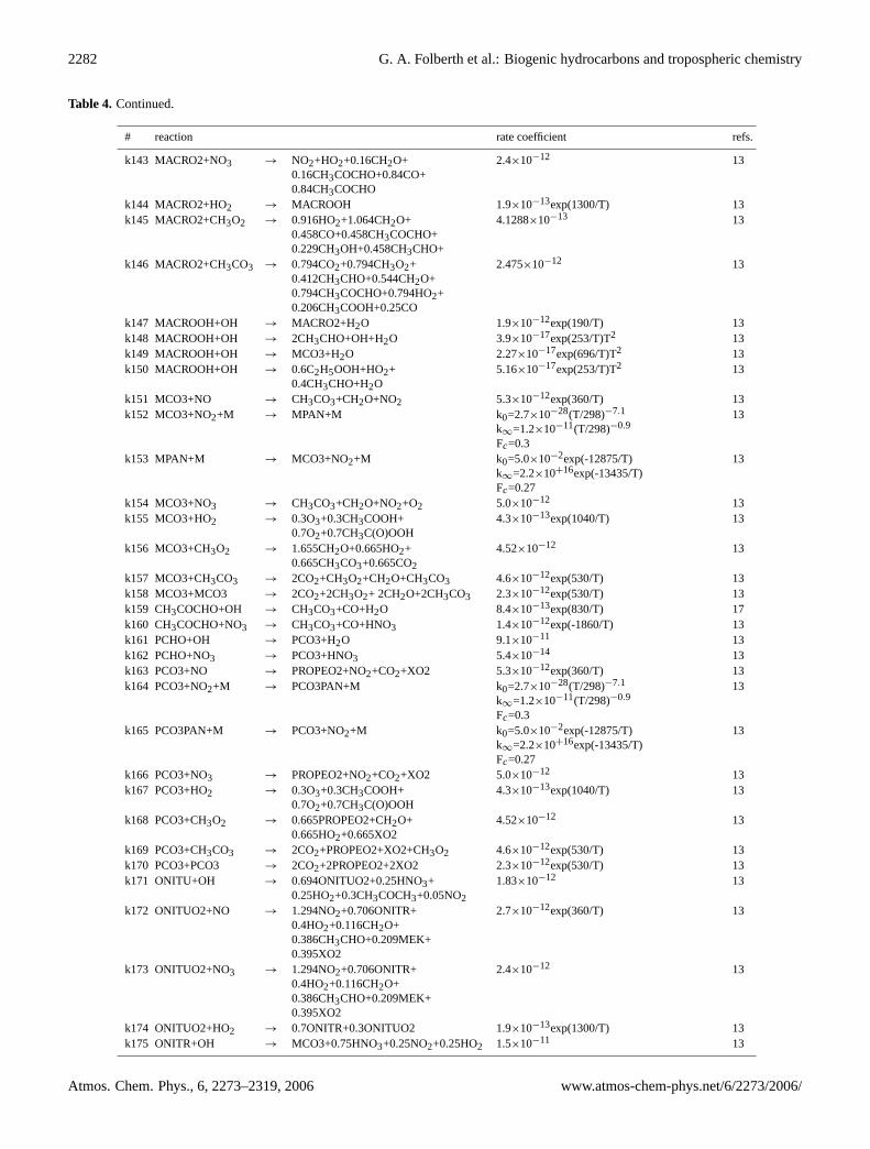
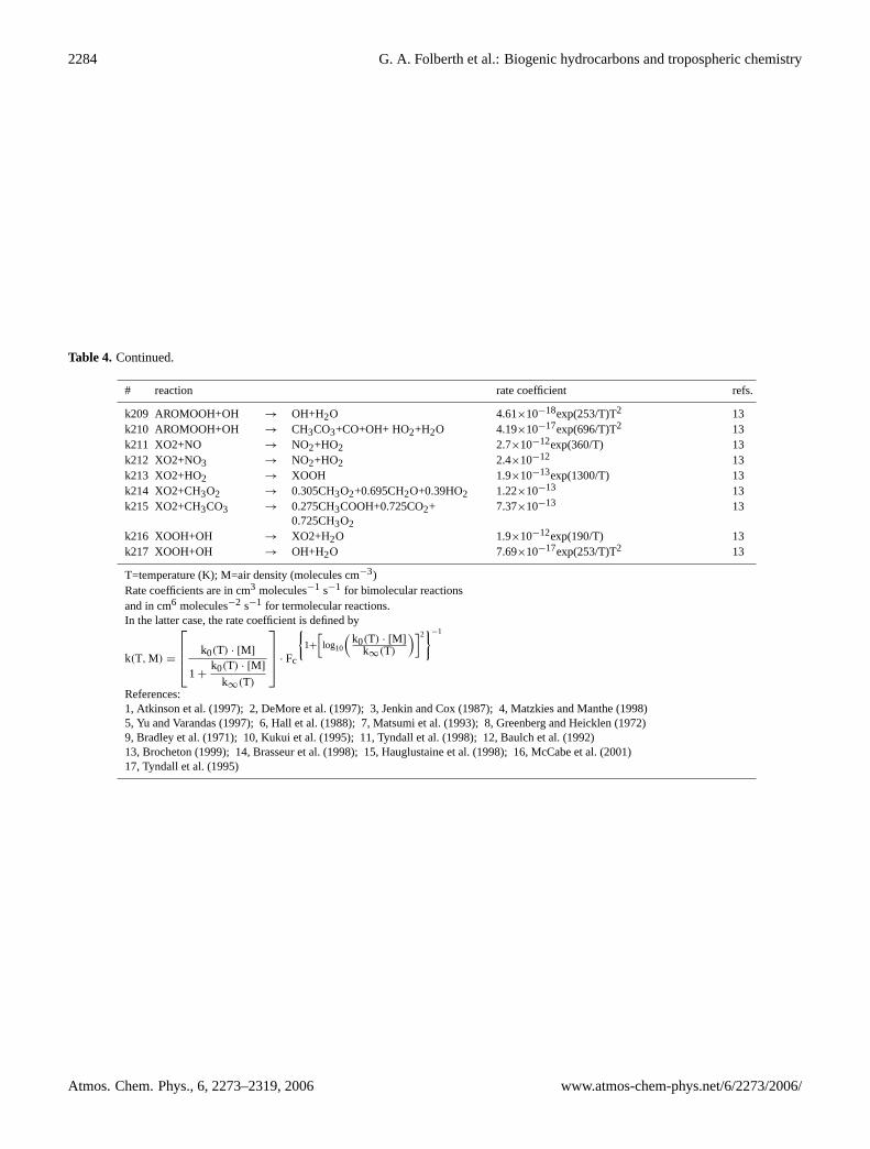
T=temperature (K); M=air density (molecules cm−3)Rate coefficients are in cm3 molecules−1 s−1 for bimolecular reactionsand in cm6 molecules−2 s−1 for termolecular reactions.In the latter case, the rate coefficient is defined by
k(T, M) =
k0(T) · [M]
1 +k0(T) · [M]
k∞(T)
· Fc
{1+
[log10
(k0(T) · [M]
k∞(T)
)]2}−1
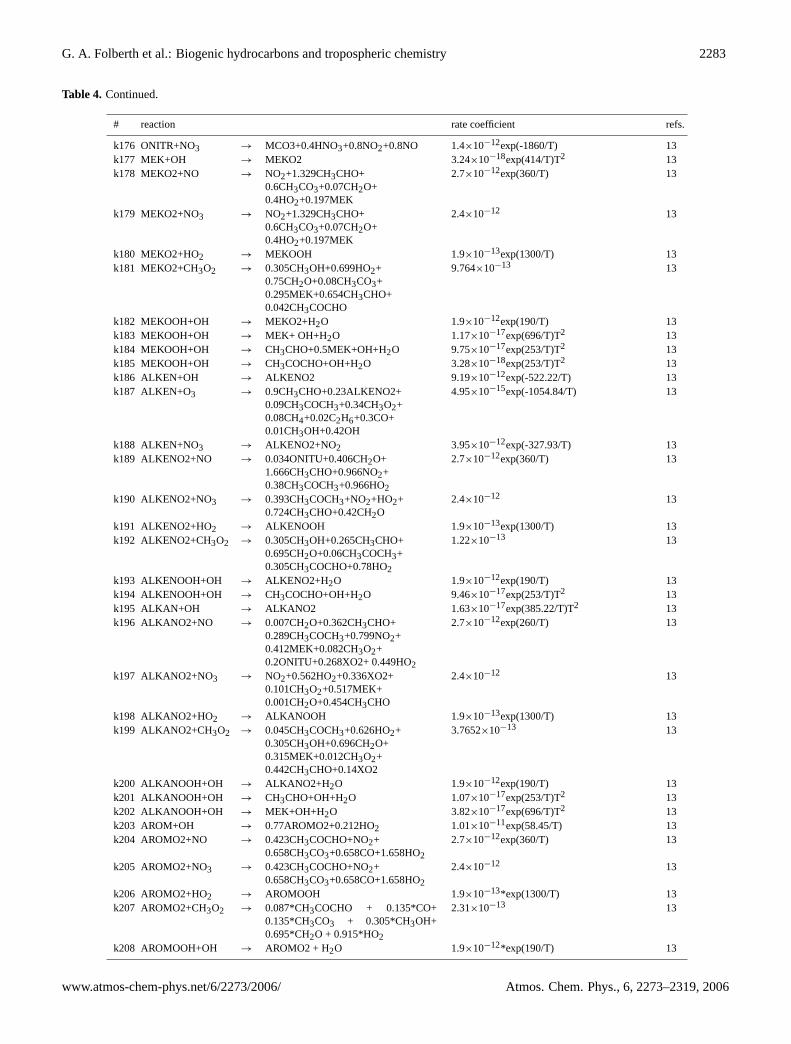
References:1, Atkinson et al.(1997); 2, DeMore et al.(1997); 3, Jenkin and Cox(1987); 4, Matzkies and Manthe(1998)5, Yu and Varandas(1997); 6, Hall et al.(1988); 7, Matsumi et al.(1993); 8, Greenberg and Heicklen(1972)9, Bradley et al.(1971); 10,Kukui et al.(1995); 11,Tyndall et al.(1998); 12,Baulch et al.(1992)13,Brocheton(1999); 14,Brasseur et al.(1998); 15,Hauglustaine et al.(1998); 16,McCabe et al.(2001)17,Tyndall et al.(1995)
Atmos. Chem. Phys., 6, 2273–2319, 2006 www.atmos-chem-phys.net/6/2273/2006/

G. A. Folberth et al.: Biogenic hydrocarbons and tropospheric chemistry 2285
The LMDz version used in this study (referred to as 3.3)has a horizontal resolution of 3.8 degrees in longitude and2.5 degrees in latitude (96×72 grid cells). The model iscomposed of 19 vertical levels onσ -p coordinates extendingfrom the surface to 3 hPa. Also higher-resolution versions ofLMDz have been developed and applied recently (e.g.Baueret al., 2004).
The primitive equations in the GCM are solved with a3 min time-step, large-scale transport of tracers is carriedout every 15 min, and physical processes are calculated at a30 min time interval. For a more detailed description and anextended evaluation of the GCM we refer to the work of, e.g.,Le Treut et al.(1994) andHarzallah and Sadourny(1995).Recently,Hauglustaine et al.(2004) have coupled LMDz tothe tropospheric chemistry model INCA, during which theGCM has been reevaluated.
2.2 The INCA-NMHC chemistry and aerosol model
IN teraction withChemistry andAerosols (INCA) is coupledon-line to the LMDz general circulation model. INCA pre-pares the surface and in situ emissions, calculates dry de-position and wet scavenging rates, and integrates in timethe concentration of atmospheric species with a time step of30 min. INCA uses a sequential operator approach, a methodgenerally applied in chemistry-transport-models (Muller andBrasseur, 1995; Brasseur et al., 1998; Wang et al., 1998a;Poisson et al., 2000). The INCA-NMHC version appliedin this study is based on an earlier version which was de-veloped to represent the background chemistry of the tropo-sphere (Hauglustaine et al., 2004). Results from this versionof the model related to the impact of chemistry on the budgetof CO2 have been published byFolberth et al.(2005).
2.2.1 Chemistry
The version of INCA used in this study includes a compre-hensive photochemical scheme originally intended to repre-sent the photochemistry of the troposphere in regional scalechemistry-transport models. In addition to the CH4–NOx–CO–O3 photochemistry representative of the troposphericbackground, INCA, in its NMHC-implementation, also takesinto account the photochemical oxidation pathways of non-methane hydrocarbons (NMHC) and non-methane volatileorganic compounds (NMVOC) from natural and anthro-pogenic sources as well as their photochemical oxidationproducts. The model can be applied to calculate the distri-bution of tropospheric ozone and its precursors, but due tothe comprehensive chemistry scheme the model is also suitedto be used in studies of biosphere-atmosphere interrelationand the impact of a changing biosphere on the global cli-mate. The species included in this more extensive version ofLMDz-INCA are summarized in Tab.1. We consider onlyone photochemical family (Ox=O3 + O(1D) + O(3P)), and
for species with very short photochemical lifetimes transportis not taken into account.
Tables1, 2, 3, and4 summarize the chemical scheme inLMDz-INCA. The scheme includes a total of 83 species, 58of which are subject to transport. In INCA-NMHC short-chained NMVOC are treated explicitly whereas a lump-ing approach is applied in the case of higher NMVOC asproposed byBrocheton(1999). Alkanes up to three car-bon atoms (C3) per molecule are treated explicitly includingmethane, ethane, and propane. All C4- and higher alkanesare lumped into one artificial species (C+
4 -alkanes). Like-wise, the model distinguishes ethene, propene, and C+
4 -alkenes. The isoprene oxidation pathway has been repre-sented with some complexity, comparable to the one pro-posed byPoschl et al.(2000) including explicitly the ma-jor oxidation products methyl vinyl ketone and methacrolein;all higher isoprenoid species are lumped into one group towhich we refer to as “terpenes”. INCA-NMHC includestwo alcohols (methanol and C+2 -alcohols, eleven hydroper-oxides, one group representing organic acids, three aldehydespecies (formaldehyde, acetaldehyde including higher mono-carboxy aldehydes, and a group representing higher aldehy-des produced by terpene oxidation), three ketones (acetone,methyl ethyl ketone, and methyl vinyl ketone), four speciesrepresenting peroxy acetyl nitrate (PAN) and analogues, twogeneral organic nitrate groups (organic nitrates with low orhigh reactivity toward OH), as well as the corresponding or-ganic radicals arising in the oxidation of the above species(cf. Tables1 and4). Lumping in all cases follows the gen-erally applied method of grouping individual compounds bytheir reactivity toward the OH-radical while also taking intoaccount compound groups, molecular weights, and atmo-spheric abundances (for a general description of these meth-ods see, e.g.,Stockwell et al., 1997).
43 photolytic reactions (Table2), 217 thermochemical re-actions (Table4), and 4 heterogeneous reactions (Table3) aretaken into account by the model. The set of reactions and re-action rates is based on the scheme ofBrocheton(1999). Allreaction rates have been reviewed and updated with respectto the compilations ofAtkinson et al.(1997) and DeMoreet al. (1997) as well as subsequent updates (Sander et al.,2000, 2002). The reaction rates are calculated by the modelat each time interval on the basis of temperature, pressure,and water vapour distribution provided by the GCM.
Pretabulated clear-sky photolysis frequenciesj are usedto determine the values at each time step and model grid cellby means of a multivariate log-linear interpolation througha Taylor series expansion (Burden and Faires, 1985). Thislook-up table is prepared with the Troposphere-Ultraviolet-Visible (TUV) model (version 4.1) fromMadronich andFlocke(1998) using a pseudo-spherical 16 stream discrete-ordinate method. The effect of cloudiness is taken intoaccount according toChang et al.(1987) as described byBrasseur et al.(1998). Further details can be found in
www.atmos-chem-phys.net/6/2273/2006/ Atmos. Chem. Phys., 6, 2273–2319, 2006
2286 G. A. Folberth et al.: Biogenic hydrocarbons and tropospheric chemistry
Hauglustaine et al.(2004). Where no spectral data is avail-able for a specific species to be used with TUV we as-sume the photolysis frequencies to be linearly dependent onchemically similar compounds (cf. Table2). The LMDz-INCA chemical scheme includes four heterogeneous reac-tions (Table3) following the recommendations ofJacob(2000) and using the monthly averaged sulfate aerosol fieldsfrom Boucher et al.(2002) to determine the aerosol distribu-tion as discussed byHauglustaine et al.(2004). The NMHC-version of LMDz-INCA uses the identical parameterizationfor the representation of these processes.
The mechanism implicitly accounts for a carbon lossthrough formation of secondary organic aerosols (SOA). Thistropospheric carbon sink is taken into account in the schemeas a carbon imbalance for specific reactions in the terpeneoxidation pathway. The estimate of the global carbon sink asderived with LMDz-INCA amounts to approximately 39%(∼37 Tg C yr−1) of the total annual carbon surface flux emit-ted as terpenes. Our estimate seems in satisfactory agreementwith the calculated variation of the global annual SOA pro-duction of 2.5 to 44 Tg C yr−1 for the biogenically producedSOA (Tsigaridis and Kanakidou, 2003). Note that explicitsecondary organic aerosol formation is not calculated in thecurrent implementation of LMDz-INCA and SOA are not in-cluded in the INCA species inventory.
Interactive calculation of chemistry and transport ofspecies extends up to the upper model level. However, inthe current version of INCA no chlorine or bromine chem-istry is taken into account and heterogeneous reactions on po-lar stratospheric clouds (PCS) is not yet considered. There-fore, ozone concentrations are relaxed toward observationsat the uppermost model levels at each time step applying arelaxation time constant of ten days above the 380K poten-tial temperature surface. The ozone observations are takenfrom the monthly mean 3-D climatologies ofLi and Shine(1995). Further details and an evaluation of the stratosphericboundary conditions in INCA can be found inHauglustaineet al. (2004); the NMHC version of INCA applies the sameapproach.
Forward integration in time of the chemical equations isconducted on the basis of five possible numerical algorithmswith a time step of 30 minutes as described byHauglustaineet al.(2004). In the current configuration of LMDz-INCA weapply the explicit Euler forward algorithm (Brasseur et al.,1999) for the integration of long-lived species (marked “l”in Table 1) and the implicit Euler backward with Newton-Raphson iteration scheme for all other species (marked “s”in Table1). A species to be long-lived in the above sense andsuitable for the less resourceful numerical algorithm requiresthe mean atmospheric lifetime of this species to be at least afew weeks.
2.2.2 Emissions
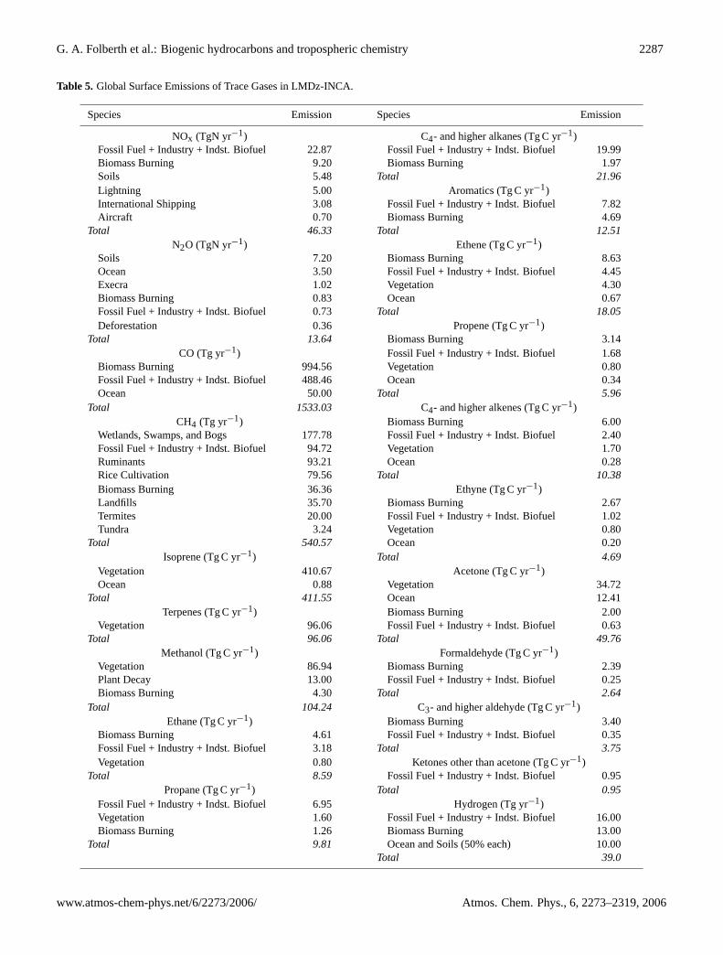
Surface emission inventories have been compiled for this ver-sion of LMDz-INCA using the same methods of data prepa-ration as described inHauglustaine et al.(2004). These in-ventories are based on various compilations, with the excep-tion of the biogenic surface source. Biogenic surface emis-sions were prepared using a global vegetation model whichincludes a biogenic emission module. Table5 summarizesthe emission magnitude for the individual species that areconsidered in the version of LMDz-INCA and used in thecurrent study.
LMDz-INCA uses anthropogenic emissions (industry, fos-sil fuel, and industrial biofuel) based on the EDGAR v3.2and EDGAR v2.0 emission databases. Anthropogenicsources for nitrogen oxides (NOx), carbon monoxide (CO),and methane (CH4) are introduced on the basis of the es-timates provided in EDGAR v3.2 (Olivier and Berdowski,2001) representative of the year 1995. The CO global emis-sions are rescaled to the values given byPrather et al.(2001).In addition, the LMDz-INCA emission inventory also in-cludes NOx emissions from oceangoing ships based onCor-bett et al.(1999) and NOx aircraft emissions based on theANCAT/EC2 inventory (Gardner et al., 1998).
At the time of creation of the current LMDz-INCA emis-sion inventory the more recent version EDGAR v3.2 didnot yet include NMVOC emissions on a per-compound ba-sis. Therefore, it was decided to use anthropogenic NMVOCemission estimates as given by the EDGAR v2.0 database(Olivier et al., 1996) which includes estimates for individualcompounds. NMVOC emissions based on EDGAR v2.0 arerepresentative of the year 1990 and include alkanes (C2H6,C3H8, C+
4 -alkanes), alkenes and alkynes (C2H4, C3H6, C+
4 -alkenes, C2H2), aromatics, aldehydes (CH2O, CH3CHOplus higher aldehydes) as well as ketones (CH3COCH3 andhigher ketones, methylethyl ketone, methylvinyl ketone).Species explicitly included in EDGAR v2.0 that are not ex-plicit in LMDz-INCA were aggregated into the specific com-pound group based on their individual molecular weights,their reactivity towards the hydroxyl radical, and their rel-ative atmospheric abundances.
Biomass burning emissions are introduced according tothe satellite based inventory developed byVan der Werfet al.(2003), averaged over the period 1997–2001. This dataset is used to provide the geographical distribution and sea-sonal variation for each compound. Domestic biofuel useand agricultural waste burning emissions are also included inthe biomass burning category and are based on the EDGARdatabase. Emission factors compiled byAndreae and Merlet(2001) are then used to derive the emission magnitude of thebiomass burning surface flux for the individual compounds.
NO soil emissions are introduced on the basis ofYiengerand Levy II(1995), emissions of CH4 from rice paddies, wet-lands, termites, wild animal and ruminants, and the oceanare taken fromFung et al.(1991), and emissions of N2O
Atmos. Chem. Phys., 6, 2273–2319, 2006 www.atmos-chem-phys.net/6/2273/2006/
G. A. Folberth et al.: Biogenic hydrocarbons and tropospheric chemistry 2287
Table 5. Global Surface Emissions of Trace Gases in LMDz-INCA.
Species Emission Species Emission
NOx (TgN yr−1) C4- and higher alkanes (Tg C yr−1)Fossil Fuel + Industry + Indst. Biofuel 22.87 Fossil Fuel + Industry + Indst. Biofuel 19.99Biomass Burning 9.20 Biomass Burning 1.97Soils 5.48 Total 21.96Lightning 5.00 Aromatics (Tg C yr−1)International Shipping 3.08 Fossil Fuel + Industry + Indst. Biofuel 7.82Aircraft 0.70 Biomass Burning 4.69
Total 46.33 Total 12.51N2O (TgN yr−1) Ethene (Tg C yr−1)
Soils 7.20 Biomass Burning 8.63Ocean 3.50 Fossil Fuel + Industry + Indst. Biofuel 4.45Execra 1.02 Vegetation 4.30Biomass Burning 0.83 Ocean 0.67Fossil Fuel + Industry + Indst. Biofuel 0.73 Total 18.05Deforestation 0.36 Propene (Tg C yr−1)
Total 13.64 Biomass Burning 3.14CO (Tg yr−1) Fossil Fuel + Industry + Indst. Biofuel 1.68
Biomass Burning 994.56 Vegetation 0.80Fossil Fuel + Industry + Indst. Biofuel 488.46 Ocean 0.34Ocean 50.00 Total 5.96
Total 1533.03 C4- and higher alkenes (Tg C yr−1)CH4 (Tg yr−1) Biomass Burning 6.00
Wetlands, Swamps, and Bogs 177.78 Fossil Fuel + Industry + Indst. Biofuel 2.40Fossil Fuel + Industry + Indst. Biofuel 94.72 Vegetation 1.70Ruminants 93.21 Ocean 0.28Rice Cultivation 79.56 Total 10.38Biomass Burning 36.36 Ethyne (Tg C yr−1)Landfills 35.70 Biomass Burning 2.67Termites 20.00 Fossil Fuel + Industry + Indst. Biofuel 1.02Tundra 3.24 Vegetation 0.80
Total 540.57 Ocean 0.20Isoprene (Tg C yr−1) Total 4.69
Vegetation 410.67 Acetone (Tg C yr−1)Ocean 0.88 Vegetation 34.72
Total 411.55 Ocean 12.41Terpenes (Tg C yr−1) Biomass Burning 2.00
Vegetation 96.06 Fossil Fuel + Industry + Indst. Biofuel 0.63Total 96.06 Total 49.76
Methanol (Tg C yr−1) Formaldehyde (Tg C yr−1)Vegetation 86.94 Biomass Burning 2.39Plant Decay 13.00 Fossil Fuel + Industry + Indst. Biofuel 0.25Biomass Burning 4.30 Total 2.64
Total 104.24 C3- and higher aldehyde (Tg C yr−1)Ethane (Tg C yr−1) Biomass Burning 3.40
Biomass Burning 4.61 Fossil Fuel + Industry + Indst. Biofuel 0.35Fossil Fuel + Industry + Indst. Biofuel 3.18 Total 3.75Vegetation 0.80 Ketones other than acetone (Tg C yr−1)
Total 8.59 Fossil Fuel + Industry + Indst. Biofuel 0.95Propane (Tg C yr−1) Total 0.95
Fossil Fuel + Industry + Indst. Biofuel 6.95 Hydrogen (Tg yr−1)Vegetation 1.60 Fossil Fuel + Industry + Indst. Biofuel 16.00Biomass Burning 1.26 Biomass Burning 13.00
Total 9.81 Ocean and Soils (50% each) 10.00Total 39.0
www.atmos-chem-phys.net/6/2273/2006/ Atmos. Chem. Phys., 6, 2273–2319, 2006

2288 G. A. Folberth et al.: Biogenic hydrocarbons and tropospheric chemistry
are based onBouwman and Taylor(1996) andKroeze et al.(1999) for continental emissions and onNevison and Weiss(1995) for the oceanic N2O surface flux. NO emissions fromlightning are calculated interactively in LMDz-INCA on thebasis of the occurrence of convection and cloud top heights.The parameterization of NO from lightning sources as it isused in LMDz-INCA is discussed in more detail byJourdainand Hauglustaine(2001) andHauglustaine et al.(2004).
Biogenic emissions of isoprene, terpenes, methanol, andacetone have been prepared with the dynamical globalvegetation model ORCHIDEE (Organizing Carbon andHydrology inDynamicEcosystEms) (Krinner et al., 2005).ORCHIDEE essentially includes three different components,namely the surface-vegetation-atmosphere transfer schemeSECHIBA (Ducoudre-De Noblet et al., 1993; de Rosnay andPolcher, 1998), the dynamic global vegetation model LPJ(Sitch et al., 2003), and STOMATE (Saclay-Toulouse-OrsayModel for theAnalysis ofTerrestrialEcosystems), a newlydeveloped model simulating plant phenology and carbon dy-namics. For a detailed description and extended evaluationof ORCHIDEE and the new carbon dynamics model STOM-ATE we refer to the paper byKrinner et al.(2005).
In order to calculate NMVOC surface fluxes from the ter-restrial biosphere, a biogenic emission module has recentlybeen integrated into ORCHIDEE. The calculation is basedon the emission model byGuenther et al.(1995) and usesinput from ORCHIDEE for the key parameters (leaf area in-dex, PFT distribution, specific leaf weight, etc.). This modeltakes into account changes in the flux strength due to leaftemperature, photosynthetically active radiation (direct anddiffuse), and leaf ageing. A detailed description and evalu-ation of the terrestrial NMVOC emission model is given byLathiere et al..
Warneke et al.(1999) first suggested a significant sourceof methanol from decaying plant matter and recent esti-mates of its magnitude range between 4 and 17 Tg C yr−1
(Singh et al., 2000; Heikes et al., 2002; Galbally and Kirstine,2002). The LMDZ-INCA emission inventory includes bio-genic methanol emissions deriving from plant decay with aglobal source strength of 13 Tg C yr−1. It is assumed that thismethanol source collocates with methanol emissions fromthe terrestrial vegetation.
LMDz-INCA takes into account oceanic emissions of COand several NMVOC (cf. Tab.5 for compounds that pos-sess oceanic sources). The spatial distribution and variationin time of oceanic CO emissions is based onErickson andTaylor (1992) and scaled to a global mean of 50 Tg C yr−1
(Prather et al., 2001). It was furthermore assumed that theglobal geographic distribution of oceanic NMVOC emis-sions equals the global oceanic CO source distribution. Theoceanic NMVOC emission magnitude is based onJacobet al.(2002) in case of acetone and on the work ofBonsanget al. (1992) andBonsang and Boissard(1999) for all otherNMVOC that posses non-zero oceanic sources in the LMDz-INCA emission inventory.
2.3 Dry deposition and wet removal
Dry deposition in LMDz-INCA is based on the resistance-in-series approach (Wesely, 1989; Walmsley and Wesely, 1996;Wesely and Hicks, 2000). Deposition velocities (vd) are cal-culated at each time step according to:
vd =1
Ra + Rb + Rc, (1)
where Ra, Rb, and Rc (s/m) are the aerodynamic, quasi-laminar, and surface resistance, respectively.Ra and Rb aredetermined on the basis ofWalcek et al.(1986). The sur-face resistance calculation for all species included in LMDz-INCA is based on their temperature dependent Henry’s LawEquilibrium Constant and reactivity factor for the oxidationof biological substances. Henry’s Law Coefficients tabu-lated for standard conditions have been taken fromSander(1999) and reactivity factors are taken fromWesely(1989)andWalmsley and Wesely(1996). The vegetation map clas-sification ofDe Fries and Townshend(1994), interpolated tothe model grid and redistributed into the classification ofWe-sely(1989), is used to parameterize land use dependencies ofthe surface resistanceRc. A complete list of species that aresubject to dry deposition is given in Table1. During the tran-sition from LMDz-INCA-CH4 to LMDz-INCA-NMHC theparameterization of dry deposition in the model has under-gone some revision taking into account recent work (see cf.,e.g.,Ganzeveld et al., 1998; Wesely and Hicks, 2000).
Wet scavenging in INCA is parameterized as a first-orderloss process as proposed byGiorgi and Chameides(1985):
d
dtCg = −βCg, (2)
whereCg is the gas-phase concentration of the consideredspecies andβ is the scavenging coefficient (1/s). Wet scav-enging associated with large scale stratiform precipitation iscalculated adopting the falling raindrop approach (Seinfeldand Pandis, 1998) and wet removal of soluble species byconvective precipitation is calculated as part of the upwardconvective mass flux on the basis of a modified version ofthe scheme proposed byBalkanski et al.(1993). INCA cal-culates wet scavenging of soluble species for convective andstratiform precipitation separately. Nitric acid is used as areference and the scavenging rate of any other species sub-ject to wet removal is scaled to the scavenging rate of HNO3according to the temperature dependent Henry’s Law Equi-librium Constant on the basis ofSeinfeld and Pandis(1998)using standard condition Henry’s Law Coefficients from theliterature (Sander, 1999). Table1 provides a list of all speciessubject to wet removal in this version of LMDz-INCA. Fora more detailed description and evaluation of both the drydeposition and wet scavenging parameterization in LMDz-INCA we refer to the paper ofHauglustaine et al.(2004).In the version of LMDz-INCA used in this study the sameschemes have been applied.
Atmos. Chem. Phys., 6, 2273–2319, 2006 www.atmos-chem-phys.net/6/2273/2006/

G. A. Folberth et al.: Biogenic hydrocarbons and tropospheric chemistry 2289
3 Model evaluation
We present here a general evaluation of the LMDz-INCAmodel in its NMHC version using a simulation which is rep-resentative of the 1990s. During development the model hasbeen run almost consecutively for more than 20 model yearsbefore a spin-up run for this study was initialized. A sixmonths spin-up was then conducted from July to Decemberusing the restart files of the last development run. After thisspin-up period the model has been run for another 24 con-secutive months, the last 12 months have been used in theanalysis. This approach was chosen to ensure that even long-lived species such as methane have reached equilibrium.
The large amount of species considered in this model andthe still rather sparse observational data available from mea-surement campaigns only allow us to discuss the major as-pects of global tropospheric chemistry in this evaluation ofthe model performance. Although the spatial distributionand time evolution of more than 80 species are calculatedby LMDz-INCA, the discussion shall be focused on the keyspecies and selected NMVOC. CO concentrations are eval-uated by comparison with surface climatologies fromNov-elli et al. (2003), other species simulated by LMDz-INCAincluding hydrocarbons, acetone, NOx, PAN, and HNO3are compared to observations from various aircraft missionsbased on the data compilation byEmmons et al.(2000) andreferences therein. Finally, calculated ozone concentrationsare evaluated by comparison with climatological ozonesondeobservations (Logan, 1999).
3.1 Carbon monoxide
Direct surface emission deriving from fossil fuel combus-tion as well as biomass burning are the most important COsources in the atmosphere. In addition, carbon monoxide isproduced in situ by oxidation of methane and non-methanehydrocarbons in the entire troposphere.
Figure1 shows the monthly mean carbon monoxide sur-face mixing ratio for January and July. CO is most abun-dant near the surface sources of the tropics and the north-ern midlatitudes as well as during the northern hemisphericwinter when its photochemical lifetime is increased owing toa decrease in the OH abundance and weak vertical mixing.Predicted mixing ratios reach 300 ppb over these regions.During the summer months CO concentrations decrease sig-nificantly in the photochemically more active atmosphere,mostly due to a strong increase in OH.
In the tropics the seasonal cycle of CO is controlled to alarge extent by the seasonality of biomass burning, whichaccount for half of the direct CO emissions. Biomass burn-ing is most intense during the dry season (December–Aprilin the northern tropics, July – October in the southern trop-ics). Over these areas with intense biomass burning (tropicalregions of Africa and South America) the model calculatesmaximum mixing ratios in the range of 200 to 300 ppb. In
Fig. 1. Carbon monoxide surface mixing ratio for January and July(ppbv).
the marine boundary layer of the southern hemisphere, back-ground CO concentrations as predicted by LMDz-INCA aregenerally lower than 70 ppb.
Simulated monthly mean carbon monoxide concentrationsnear the surface are compared with climatologies from ob-servations for 18 selected stations from the CMDL network(Novelli et al., 2003) in Fig. 2. Measurements are depictedas monthly means including their standard deviation over theperiod of record (5 to 10 years, depending on the station).
The model captures well both the absolute values and theseasonal variation of CO mixing ratios in most cases, exceptfor a tendency to overestimate CO by up to 20 ppb at southernmid and high latitudes (cf. Cape Grim, South Pole). The gen-erally higher CO concentrations in the northern hemisphericmid- and high latitudes (e.g., Alert, Baltic Sea, Mace Head,Bermuda) are well captured by the model at virtually all sites,
www.atmos-chem-phys.net/6/2273/2006/ Atmos. Chem. Phys., 6, 2273–2319, 2006

2290 G. A. Folberth et al.: Biogenic hydrocarbons and tropospheric chemistry
Fig. 2. Comparison of observed and calculated monthly mean CO mixing ratios at the surface. Black circles and solid lines denote observedvalues fromNovelli et al. (2003) averaged over 5 to 10 years depending on the sites; vertical bars are standard deviations. Blue opendiamonds and heavy dashed lines represent monthly mean CO concentrations calculated by the model. Solid thin blue lines depict the dailyvariation in the model data.
Atmos. Chem. Phys., 6, 2273–2319, 2006 www.atmos-chem-phys.net/6/2273/2006/
G. A. Folberth et al.: Biogenic hydrocarbons and tropospheric chemistry 2291
both in terms of seasonality and magnitude. The model alsoshows a good agreement with tropical sites in the northernhemisphere (e.g., Easter Islands, Canary Islands, Midway).The model reproduces the seasonal cycle and spring maxi-mum in the southern tropics (Ascension Island and Ameri-can Samoa) fairly well, which is governed by the seasonalbiomass burning emissions (July to October in the southernhemisphere). However, the peak in CO is one month early atAscension and overestimated but in phase at the Samoa site.
The comparison suggests that the model is capable of re-producing CO concentration well at locations where wellconstrained anthropogenic CO sources contribute a signifi-cant portion of the emissions (practically all of the northernhemisphere). In the southern hemisphere, where CO concen-trations are generally lower and are dominated by biomassburning and, to some extent at southern high latitudes, evenby the oceanic source, the model has a tendency of overesti-mating CO concentrations. This is most likely due to the CObiomass burning emission set, but could also be caused byan overestimate of the VOC emissions with subsequent in-situ formation of CO by photooxidation or an underestimateof the concentration of hydroxyl radicals near the surface atthese locations. In general though, the tendency to underes-timate CO concentrations, persistent in many current chem-istry models both taking and not taking into account VOCphotochemistry (cf., e.g.,Hauglustaine et al., 1998; Poissonet al., 2000; Bey et al., 2001; Hauglustaine et al., 2004), is notdiscernible in the NMHC version of LMDz-INCA, which wetentatively attribute to the spatial and time variability of theOH abundance well reproduced by the model (cf. Sect.3.2).
3.2 Hydroxyl radical and methane concentration
OH is most abundant in the tropical lower and midtroposphere reflecting high levels of ultraviolet radiationand water vapour. OH concentrations can reach 20 to30×105 molecules cm−3 in this atmospheric domain and de-crease with altitude due to a decline in water vapour abun-dance.
The global mean OH concentration as calculated bythe model can be evaluated by using the methylchloro-form (CH3CCl3) lifetime as a proxy (Spivakovsky et al.,1990; Prinn et al., 1995). Spivakovsky et al.(2000) cal-culated a global mean atmospheric lifetime of 4.6 yearsfor methylchloroform, in close agreement withPrinn et al.(1995). Assessing stratospheric and oceanic sinks forCH3CCl3 with corresponding lifetimes of 43 and 80 yearsrespectively,Spivakovsky et al.(2000) established a tropo-spheric methyl chloroform lifetime against OH reaction of5.5 years. Houweling et al.(1998), Wang et al.(1998a),Mickley et al. (1999), andBey et al.(2001) obtained cor-responding lifetimes of 5.3, 6.2, 7.3, and 5.1 years from theirmodel calculations, respectively. LMDz-INCA calculates atropospheric CH3CCl3 lifetime with respect to oxidation byOH of 5.5 years in excellent agreement with the estimates of
CH4 Lifetime
J F M A M J J A S O N D 6
7
8
9
10
11
12
year
s
CH3CCl3 Lifetime
J F M A M J J A S O N D 4
5
6
7
8
year
s
OH Burden
J F M A M J J A S O N D 6
7
8
9
10
11
12
105 c
m-3
O3 Burden
J F M A M J J A S O N D 240
260
280
300
320
340
360
Tg
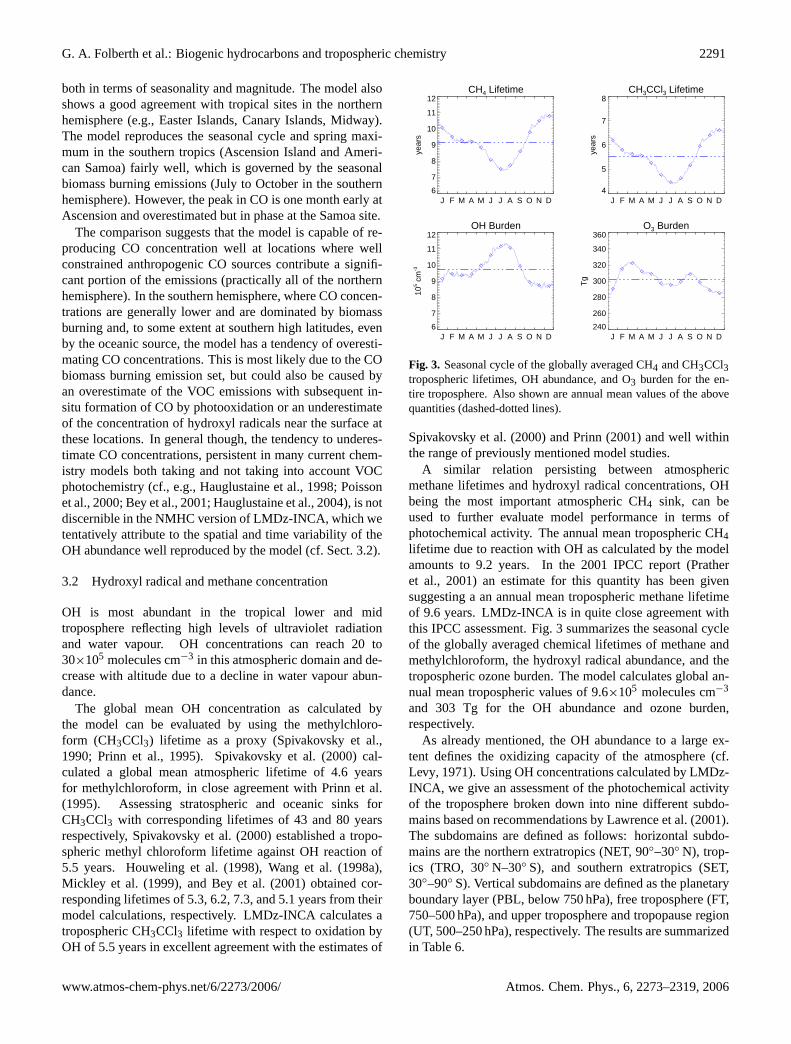
Fig. 3. Seasonal cycle of the globally averaged CH4 and CH3CCl3tropospheric lifetimes, OH abundance, and O3 burden for the en-tire troposphere. Also shown are annual mean values of the abovequantities (dashed-dotted lines).
Spivakovsky et al.(2000) andPrinn (2001) and well withinthe range of previously mentioned model studies.
A similar relation persisting between atmosphericmethane lifetimes and hydroxyl radical concentrations, OHbeing the most important atmospheric CH4 sink, can beused to further evaluate model performance in terms ofphotochemical activity. The annual mean tropospheric CH4lifetime due to reaction with OH as calculated by the modelamounts to 9.2 years. In the 2001 IPCC report (Pratheret al., 2001) an estimate for this quantity has been givensuggesting a an annual mean tropospheric methane lifetimeof 9.6 years. LMDz-INCA is in quite close agreement withthis IPCC assessment. Fig.3 summarizes the seasonal cycleof the globally averaged chemical lifetimes of methane andmethylchloroform, the hydroxyl radical abundance, and thetropospheric ozone burden. The model calculates global an-nual mean tropospheric values of 9.6×10⁵ molecules cm−3
and 303 Tg for the OH abundance and ozone burden,respectively.
As already mentioned, the OH abundance to a large ex-tent defines the oxidizing capacity of the atmosphere (cf.Levy, 1971). Using OH concentrations calculated by LMDz-INCA, we give an assessment of the photochemical activityof the troposphere broken down into nine different subdo-mains based on recommendations byLawrence et al.(2001).The subdomains are defined as follows: horizontal subdo-mains are the northern extratropics (NET, 90◦–30◦ N), trop-ics (TRO, 30◦ N–30◦ S), and southern extratropics (SET,30◦–90◦ S). Vertical subdomains are defined as the planetaryboundary layer (PBL, below 750 hPa), free troposphere (FT,750–500 hPa), and upper troposphere and tropopause region(UT, 500–250 hPa), respectively. The results are summarizedin Table6.
www.atmos-chem-phys.net/6/2273/2006/ Atmos. Chem. Phys., 6, 2273–2319, 2006

2292 G. A. Folberth et al.: Biogenic hydrocarbons and tropospheric chemistry
Table 6. Break-down of annual average hydroxyl radical concentra-tions classified by tropospheric subdomains (105 molecules cm−3).Horizontal domains: northern extratropics (NET, 90◦–30◦ N),tropics (TRO, 30◦N–30◦ S), southern extratropics (SET, 30◦–90◦ S); vertical domains: planetary boundary layer (PBL, below750 hPa), free troposphere (FT, 750–500 hPa), upper troposphereand tropopause region (UT, 500–250 hPa), respectively. The rowsand columns denoted byTOT andTOT , respectively, refer to themean calculated over the specific horizontal layer or altitude range.
subdomain PBL FT UT TOT
NET 9.0 6.4 5.6 7.8TRO 16.6 10.7 7.7 12.5SET 5.3 4.4 4.5 5.4TOT 11.9 8.1 6.4 9.6
From Table6 it can be seen that the tropical planetaryboundary layer has the highest oxidative capacity of all tro-pospheric subdomains with an annual mean OH abundanceof 16.6×10⁵ molecules cm−3. The oxidative capacity calcu-lated by the model decreases with increasing altitude, consis-tent with the current knowledge. Viewed over the entire alti-tude range, the tropical troposphere shows the highest oxida-tive capacity, in the southern extratropical troposphere OHconcentrations are on average significantly lower.
Methane itself is a prognostic tracer in LMDz-INCA. Themodel takes into account various primary sources of CH4 (cf.Table 5), transport and mixing, tropospheric-stratosphericexchange, and atmospheric oxidation. A global sink of ap-proximately 30 Tg yr−1 due to consumption of CH4 bymethanotropic bacteria in soil has been identified (cf., e.g.,Prather et al., 2001). The uncertainties around this processesare still quite high and are expressed in terms of an uncer-tainty factor of 2. This process, though, is not accountedfor in our model at the present. The sink would account forapproximately 5% of the global primary source of methane.Non-neglible but small on the global scale, this sink couldpotentially be of importance on the regional scale, since it isconcentrated over the continental areas and varies with soilconditions.
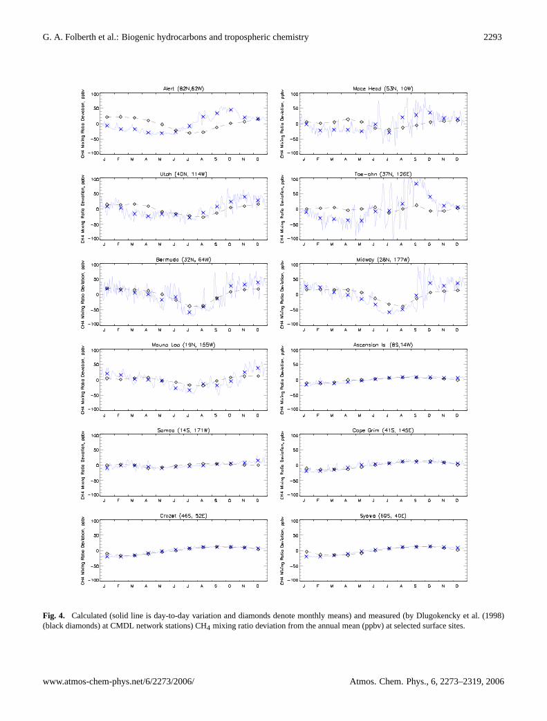
The methane concentration at the surface as depicted inFig. 4 exhibits a pronounced seasonal cycle in both theCMDL measurements and the model with a minimum dur-ing the local summer months when photochemical depletionvia reaction with OH is most active. The observed magni-tude and phase of the seasonal variation in methane is fairlywell reproduced by the model. Differences between modeland observations are most pronounced at northern midlati-tude continental stations. The agreement between model andobservations increases at stations in the tropics and the south-ern hemisphere representative of tropospheric backgroundconditions. At these stations the model shows less diurnalvariation which we contribute to a decreased influence of the
rapid photochemistry of NMVOC which also produces sig-nificant amounts of CH4. This absence of photochemistry onshort time-scales of hours or days could affect the compar-ison between climatological observations and the calculatedmethane concentration.
3.3 Nitrogen compounds
The importance of nitrogen compounds is a consequence oftheir role in the budget of other key tropospheric species,such as ozone and the hydroxyl radical. Odd nitrogen ismainly released in the form of NO, predominantly as a resultof combustion processes (fossil fuel combustion, biomassburning) and soil microbial activity. Global lightning activityalso represents a significant atmospheric source of NO. Onceemitted, NO is rapidly converted by photochemical processesinto other states of oxidation (NO2, NO3, N2O5) as well asHNO3 and organic nitrates, including peroxyacetyl nitrate(PAN).
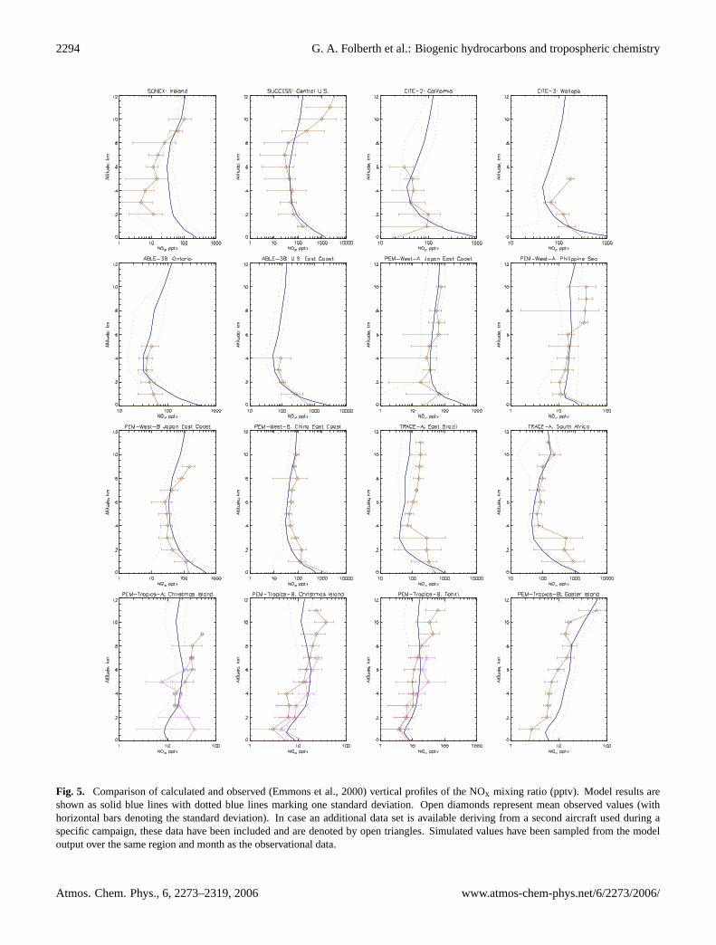
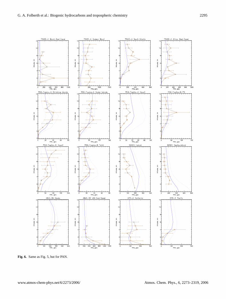
A comparison of observed and calculated profiles of NOxand PAN are shown in Figs.5 and6. The calculated NOxmixing ratio is generally in good agreement with observa-tions, given the large spatial and time variability in this short-lived species. The typically ”C-shaped” profiles with highermixing ratios in the PBL and the upper troposphere as wellas decreased mixing ratios in the free troposphere are alsowell captured. The model, however, overestimates NOx overIreland during SONEX below 8 km which could be due toan overestimate of the anthropogenic NOx source in EDGARv3.2 or the export of NOx from the continent being too strongin our model over this region. The model underestimatesNOx concentrations in the upper troposphere during SUC-CESS.
Organic nitrates in general, and in particular peroxyacetylnitrate (PAN), are chemically more stable compounds thanNOx. PAN is the most abundant organic nitrate that has beendetected in the atmosphere resulting from a variety of organicprecursors, such as isoprene, acetaldehyde, and alkanes (e.g.Roberts, 1990; Altshuller, 1993). Predominantly produced inthe PBL by reaction of peroxyacetyl radicals with NO2, PANsubsequently becomes subject to long-distance transport toremote environments and to the free troposphere, where itacts as a reservoir of NOx. Eventually, NOx is releasedfollowing thermal decomposition and photolysis (Crutzen,1979; Kasibhatla, 1993; Moxim et al., 1996). PAN lifetimesvary from a few hours in the lower troposphere, where ther-mal decomposition effectively limits its residence time, toseveral months in the free and upper troposphere. LMDz-INCA also considers PAN analogs that derive from higherNMHC as well as other bulk organic nitrate species (cf. Ta-ble 1). They generally have shorter atmospheric lifetimesand, hence, significant concentrations are found only in thePBL.
Calculated profiles of the PAN mixing ratio are mostlywithin one standard deviation of the observations, but show
Atmos. Chem. Phys., 6, 2273–2319, 2006 www.atmos-chem-phys.net/6/2273/2006/
G. A. Folberth et al.: Biogenic hydrocarbons and tropospheric chemistry 2293
Fig. 4. Calculated (solid line is day-to-day variation and diamonds denote monthly means) and measured (byDlugokencky et al.(1998)(black diamonds) at CMDL network stations) CH4 mixing ratio deviation from the annual mean (ppbv) at selected surface sites.
www.atmos-chem-phys.net/6/2273/2006/ Atmos. Chem. Phys., 6, 2273–2319, 2006
2294 G. A. Folberth et al.: Biogenic hydrocarbons and tropospheric chemistry
Fig. 5. Comparison of calculated and observed (Emmons et al., 2000) vertical profiles of the NOx mixing ratio (pptv). Model results areshown as solid blue lines with dotted blue lines marking one standard deviation. Open diamonds represent mean observed values (withhorizontal bars denoting the standard deviation). In case an additional data set is available deriving from a second aircraft used during aspecific campaign, these data have been included and are denoted by open triangles. Simulated values have been sampled from the modeloutput over the same region and month as the observational data.
Atmos. Chem. Phys., 6, 2273–2319, 2006 www.atmos-chem-phys.net/6/2273/2006/
G. A. Folberth et al.: Biogenic hydrocarbons and tropospheric chemistry 2295
Fig. 6. Same as Fig.5, but for PAN.
www.atmos-chem-phys.net/6/2273/2006/ Atmos. Chem. Phys., 6, 2273–2319, 2006

2296 G. A. Folberth et al.: Biogenic hydrocarbons and tropospheric chemistry
Fig. 7. Same as Fig.5, but for HNO3.
Atmos. Chem. Phys., 6, 2273–2319, 2006 www.atmos-chem-phys.net/6/2273/2006/

G. A. Folberth et al.: Biogenic hydrocarbons and tropospheric chemistry 2297
a tendency to underestimate PAN in regions affected bybiomass burning as during TRACE-A. A tendency to overes-timate PAN over polluted areas as during SONEX is also dis-cernible. The model seems to better reproduce PAN profilesover unpolluted remote regions (PEM-West, PEM-Tropics,TRACE-A) than over regions with a strong continental influ-ence (SONEX, ABLE). Observed PAN concentrations showa maximum between approximately 4 and 8 km dependingon the individual location. This mid-tropospheric maximumis a consequence of an increasing lifetime against thermaldecomposition with increasing altitude and a decreasing life-time against photolysis with increasing altitude. The modelqualitatively and quantitatively captures this feature reason-ably well.
Nitric acid (HNO3) in the atmosphere is produced by reac-tion of NO2 with OH and by hydrolysis of N2O5; major sinksare dry and wet deposition. Comparison of simulated verti-cal profiles of HNO3 with observations as shown in Fig.7reveals a pronounced tendency of LMDz-INCA to overesti-mate HNO3 concentrations, typically by a factor of two. Thelargest deviations are found in the upper troposphere between9 and 12 km. This problem is common to most current global3-D models of tropospheric chemistry (Hauglustaine et al.,1998; Lawrence et al., 1999; Poisson et al., 2000; Bey et al.,2001; Hauglustaine et al., 2004). However, in the NMHC im-plementation of LMDz-INCA this tendency to overestimateHNO3 concentrations seems to be less pronounced.Bey et al.(2001) have suggested partitioning of nitric acid into aerosolsas a possible explanation for this common model deficiency,since most current tropospheric chemistry model do not dif-ferentiate between gaseous and aerosol nitrate as is also thecase for LMDz-INCA. Studies byBauer et al.(2004) witha version of LMDz-INCA including such fractionation pro-cesses but without NMVOC photochemistry seem to supportthis argument. A better agreement between calculated HNO3concentrations and observations is obtained over remote re-gions, in particular during the PEM-Tropics campaigns, in-dicating that HNO3 overestimation in the model is most pro-nounced over areas with high NOx emissions.
3.4 Methanol, acetone, and other VOC
The seasonal mean methanol mixing ratio at the surface isdepicted in Fig.8 for the winter and summer seasons. Theprincipal global CH3OH source is plant growth. Methanolsurface mixing ratios as calculated by the model follow theglobal seasonal vegetation cycle with low values at mid- andhigh latitudes in the winter hemisphere, elevated levels in thesame latitudinal range in the summer hemisphere, and year-round relatively high mixing ratios over continental areas inthe tropics. The methanol mixing ratio ranges between 10and 25 ppbv over tropical South America and Africa duringthe winter season and reach 30 to 40 ppbv over SoutheastAsia and the Eastern United States during the summer sea-son.
Fig. 8. Methanol surface mixing ratio for winter and summer season(ppbv).
Calculated vertical CH3OH profiles are compared to ob-servations in Fig.9. The model shows a tendency to under-estimate the methanol mixing ratio over remote areas (ob-servations from PEM-Tropics B) where measured values canbe higher by up to a factor of 2.5 in the lower troposphere.Generally, the agreement is better at higher altitudes. On theother hand, the model seems to overestimate CH3OH signif-icantly at northern hemispheric midlatitudes as compared tomeasurements from the SONEX campaign.
Formaldehyde (CH2O) in the atmosphere originates fromvarious sources. These include fossil fuel combustion (mi-nor), biomass burning and biogenic surface emissions as wellas substantial secondary in-situ sources. This secondary pho-tochemical source derives from photooxidation of methaneand non-methane hydrocarbons, the most important of which
www.atmos-chem-phys.net/6/2273/2006/ Atmos. Chem. Phys., 6, 2273–2319, 2006

2298 G. A. Folberth et al.: Biogenic hydrocarbons and tropospheric chemistry
Fig. 9. Same as Fig.5, but for methanol.
is isoprene. Figure10 shows a comparison of the seasonalvariation in CH2O mixing ratios as calculated by the modelwith observations near the surface. Observational data hasbeen collected in the framework of the CMDL network. Mostof the available data has been collected at northern hemi-spheric midlatitudinal stations, except Zeppelin which is lo-cated at polar latitudes. The model shows a fair agreementwith the observations at several stations but considerablyunderestimates formaldehyde concentrations at Ispra, MaceHead, and Zeppelin.
Figure 11 compares simulated formaldehyde profiles toaircraft measurements for various campaigns. Profiles cal-culated by LMDz-INCA are in good agreement with ob-servations collected during SONEX which are representa-tive of near continental regions under the influence of bothprimary and secondary CH2O sources. The model showsa fairly good agreement close to the surface with observa-tions obtained during TRACE-A near Brazil. This cam-paign was conducted during September and October of 1992and covered a period of the year which is characterized byhigh net primary production of the vegetation in the south-ern hemisphere. The fairly good agreement would indicatethat the isoprene emissions calculated with ORCHIDEE forthe Amazon region are reasonable in magnitude, at least forthis period of the year. Furthermore, fairly good agreementis achieved with data gathered during the PEM-Tropics Bcampaign. The region covered by this campaign can be con-
sidered typical for remote regions of the troposphere dom-inated by background conditions, a diminished continentalinfluence that, if apparent, stems from long-range transport,and only weak local primary sources. The most pronounceddeviation between model and measurements occurs for theTRACE-A campaign at the South Atlantic location, whereLMDz-INCA seems to overestimate observed formaldehydeconcentrations in the lower and middle troposphere by up to afactor of three. This disagreement could be related to sourcesof formaldehyde or its precursors from biomass burning orbiogenic formation being too high in our emission inventorynear this region (South American continental sources).
Vertical profiles of acetone from the model and observa-tions are compared in Fig.12. Over most regions (includingthose sampled during PEM-West B and PEM-Tropics B) themodel estimates of the acetone mixing ratio agree fairly wellwith the observations. The higher levels observed during theTRACE-A campaign over Brazil and Africa, also well sim-ulated by the model, are related to acetone emissions frombiomass burning. The model captures the vertical gradientsin most cases. It generally also reproduces the acetone mix-ing ratios observed in the Asian outflow during PEM-WESTB, but significantly overestimates acetone at the near conti-nental sites measured during the SONEX campaign. How-ever, acetone profiles calculated by LMDz-INCA do agreequite well with observations obtained during the ABLE-3B(Singh et al., 1994a) experiments.
Atmos. Chem. Phys., 6, 2273–2319, 2006 www.atmos-chem-phys.net/6/2273/2006/

G. A. Folberth et al.: Biogenic hydrocarbons and tropospheric chemistry 2299
Birkenes (58N / 8E)
J F M A M J J A S O N D 0.0
0.5
1.0
1.5
2.0
CH
2O M
ixin
g R
atio
, ppb
v
Donon (49N / 7E)
J F M A M J J A S O N D 0
1
2
3
4
CH
2O M
ixin
g R
atio
, ppb
v
Ispra (46N / 9E)
J F M A M J J A S O N D 0
1
2
3
4
5
6
CH
2O M
ixin
g R
atio
, ppb
v
Kosetice (49N / 15E)
J F M A M J J A S O N D 0.0
0.5
1.0
1.5
2.0
2.5
3.0
CH
2O M
ixin
g R
atio
, ppb
v
Mace Head (53N / 10W)
J F M A M J J A S O N D 0.0
0.2
0.4
0.6
0.8
1.0
CH
2O M
ixin
g R
atio
, ppb
v
Montelibretti (42N / 13E)
J F M A M J J A S O N D 0
2
4
6
8
CH
2O M
ixin
g R
atio
, ppb
v
Rucava (56N / 21E)
J F M A M J J A S O N D 0.0
0.5
1.0
1.5
2.0
CH
2O M
ixin
g R
atio
, ppb
v
Waldhof (53N / 11E)
J F M A M J J A S O N D 0.0
0.5
1.0
1.5
2.0
2.5
3.0
CH
2O M
ixin
g R
atio
, ppb
v
Zeppelin (79N / 12E)
J F M A M J J A S O N D 0.00
0.10
0.20
0.30
0.40
CH
2O M
ixin
g R
atio
, ppb
v
Fig. 10. Same as Fig.2, but for CH2O.
The observations gathered during PEM-Tropics B indicatesurprisingly large abundances of acetone over the tropical Pa-cific (Singh et al., 2001), a region where most models previ-ously predicted quite low concentrations (cf., e.g.Hauglus-taine et al., 1998; Bey et al., 2001; Horowitz et al., 2003).These observations suggest the presence of a large natural,distributed source of oxygenated organic species as has beendiscussed byHorowitz et al.(2003). The current version ofLMDz-INCA does not seem to show the same disagreement,possibly owing to the inclusion of an oceanic source for ace-tone based on theJacob et al.(2002) recommendations.
3.5 Ozone
Figure 13 shows seasonal mean ozone mixing ratios cal-culated near the surface for the winter and summer sea-sons. Maximum mixing ratios reaching 50 to 70 ppbv arecalculated over industrialized regions of the northern hemi-sphere during summertime, where strong biogenic NMVOCsources combine with pronounced NOx concentrations (East-ern United States, Europe, Southeast Asia). Elevated ozonelevels of up to 50 ppbv are also visible over ares with in-tense biomass burning emissions in the tropical continentaldomain. In general, the ozone distribution as calculated byLMDz-INCA is in good agreement with previous studies (cf.e.g.Hauglustaine et al., 1998; Wang et al., 1998b; Poissonet al., 2000; Bey et al., 2001; Horowitz et al., 2003).
Over the oceans the ozone background mixing ratio isgenerally less than 25 ppb in both hemispheres except overthe North Pacific and the North Atlantic during wintertime,where export of O3 from the continental boundary layer isclearly visible. In regions remote from any pollution sources,such as the Central Pacific Ocean, the Indian Ocean, or theSouthern Ocean, ozone mixing ratios can drop to less than15 ppb. A summertime minimum with less than 15 ppbv ofozone is calculated over the North Pacific, where NOx con-centrations are very low while ozone destruction by photoly-sis is significant.
Figure14provides an evaluation of the surface ozone mix-ing ratio as derived by the model by comparison with mea-surements at 15 selected stations. Observational data havebeen taken from the CMDL network (cf.Komhyr et al., 1989;Oltmans et al., 1989; Oltmans and Levy II, 1992, 1994) andrepresent monthly means, averaged over the total observa-tional record at each station, which cover between 5 and 10years. In general, calculated monthly mean ozone mixingratios as well as the simulated seasonal cycle are in goodagreement with the observed values at most sites. The sim-ulated ozone mixing ratios reproduce generally well the ob-served values in subtropical regions and at midlatitudes inthe Northern Hemisphere (Mace Head, Payerne, Hohenpeis-senberg, Sable Island, Zugspitze, Mauna Loa). The modelfails to capture the arctic springtime ozone minimum at Bar-row, which has been attributed to bromine catalysed ozonedepletion events (Barrie et al., 1988; Tang and McConnell,
www.atmos-chem-phys.net/6/2273/2006/ Atmos. Chem. Phys., 6, 2273–2319, 2006

2300 G. A. Folberth et al.: Biogenic hydrocarbons and tropospheric chemistry
SONEX: East Atlantic
0 100 200 300 400CH2O, pptv
0
2
4
6
8
10
12
Alti
tude
, km
SONEX: Ireland
0 100 200 300CH2O, pptv
0
2
4
6
8
10
12
Alti
tude
, km
SONEX: Newfoundland
0 200 400 600 800CH2O, pptv
0
2
4
6
8
10
12
Alti
tude
, km
TRACE-A: Africa, West Coast
0 100 200 300 400CH2O, pptv
0
2
4
6
8
10
12
Alti
tude
, km
TRACE-A: South Atlantic
0 100 200 300 400CH2O, pptv
0
2
4
6
8
10
12
Alti
tude
, km
TRACE-A: East Brazil
0 1000 2000 3000CH2O, pptv
0
2
4
6
8
10
12
Alti
tude
, km
TRACE-A: Brazil, East Coast
0 200 400 600CH2O, pptv
0
2
4
6
8
10
12
Alti
tude
, km
PEM-Tropics-B: Hawaii
0 100 200 300 400 500CH2O, pptv
0
2
4
6
8
10
12
Alti
tude
, km
PEM-Tropics-B: Christmas Island
0 100 200 300 400 500CH2O, pptv
0
2
4
6
8
10
12
Alti
tude
, km
PEM-Tropics-B: Tahiti
0 100 200 300 400 500CH2O, pptv
0
2
4
6
8
10
12
Alti
tude
, km
PEM-Tropics-B: Easter Island
0 100 200 300CH2O, pptv
0
2
4
6
8
10
12
Alti
tude
, km
PEM-Tropics-B: Fiji
0 100 200 300 400CH2O, pptv
0
2
4
6
8
10
12
Alti
tude
, km
Fig. 11. Same as Fig.5, but for formaldehyde.
1996; Martinez et al., 1999; Wennberg, 1999). In the South-ern Hemisphere, the seasonal cycle and magnitude of ozoneis fairly well reproduced at subtropical- (American Samoa)and mid latitudes (Cape Grim), but both the seasonality andmagnitude are considerably underestimated at South Poleduring most of the year (April to November). As photo-chemistry is slow in the polar regions, a connection of thisdiscrepancy with transport processes seems likely.
The vertical distribution of the ozone mixing ratio as cal-culated by LMDz-INCA is evaluated against ozone sound-ings in Fig.15. The observations are taken from the clima-tology described byLogan(1999). The comparison confirmsthe general good agreement with the observations at most sta-tions. With only a few exceptions, model results are within10 to 15 ppb of the observed values, they are well within theirobserved variability (±1σ standard variation), and show thecorrect seasonal phase.
At high northern latitudes (Alert station) the model cap-tures the spring maximum in the lower troposphere and themaximum from May to August in the middle troposphere.The model underestimates, though, the monthly mean mix-ing ratios during spring and summer near the tropopauseand also visibly underestimates the observed variability. Theweakly developed variability in simulated upper troposphericozone as compared to the observations has been attributedto an overestimate of the tropopause height by the GCM(Hauglustaine et al., 2004) resulting in lower than observedO3 mixing ratios in the above 300 hPa region.
Seasonal variations at northern mid-latitudes are fairlywell reproduced (Hohenpeissenberg, Payerne). The timingof the ozone maximum in polluted regions (spring in theupper troposphere and a gradual shift toward the summerseason with decreasing altitude) is also generally well re-produced by the model to within the constraints offered by
Atmos. Chem. Phys., 6, 2273–2319, 2006 www.atmos-chem-phys.net/6/2273/2006/

G. A. Folberth et al.: Biogenic hydrocarbons and tropospheric chemistry 2301
Fig. 12. Same as Fig.5, but for acetone.
the observations at mid-latitude stations (Sapporo, Payerne,Boulder). A good model-to-measurement agreement over theentire troposphere is achieved at tropical (American Samoa)and at southern midlatitude (Asperton) stations.
Table7 provides an estimate of the annual ozone budgetin the troposphere (defined as the domain extending fromthe surface up to 200 hPa) as calculated with LMDz-INCA.The results indicate that sources and sinks in the troposphere
www.atmos-chem-phys.net/6/2273/2006/ Atmos. Chem. Phys., 6, 2273–2319, 2006
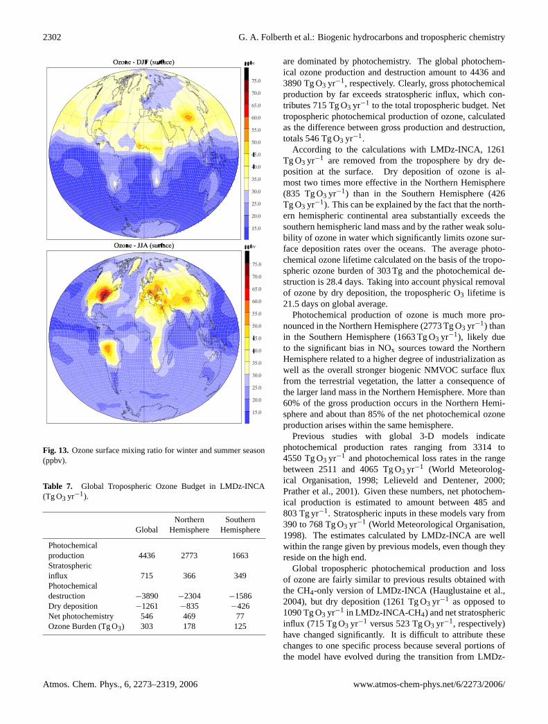
2302 G. A. Folberth et al.: Biogenic hydrocarbons and tropospheric chemistry
Fig. 13. Ozone surface mixing ratio for winter and summer season(ppbv).
Table 7. Global Tropospheric Ozone Budget in LMDz-INCA(Tg O3 yr−1).
Northern SouthernGlobal Hemisphere Hemisphere
Photochemicalproduction 4436 2773 1663Stratosphericinflux 715 366 349Photochemicaldestruction −3890 −2304 −1586Dry deposition −1261 −835 −426Net photochemistry 546 469 77Ozone Burden (Tg O3) 303 178 125
are dominated by photochemistry. The global photochem-ical ozone production and destruction amount to 4436 and3890 Tg O3 yr−1, respectively. Clearly, gross photochemicalproduction by far exceeds stratospheric influx, which con-tributes 715 Tg O3 yr−1 to the total tropospheric budget. Nettropospheric photochemical production of ozone, calculatedas the difference between gross production and destruction,totals 546 Tg O3 yr−1.
According to the calculations with LMDz-INCA, 1261Tg O3 yr−1 are removed from the troposphere by dry de-position at the surface. Dry deposition of ozone is al-most two times more effective in the Northern Hemisphere(835 Tg O3 yr−1) than in the Southern Hemisphere (426Tg O3 yr−1). This can be explained by the fact that the north-ern hemispheric continental area substantially exceeds thesouthern hemispheric land mass and by the rather weak solu-bility of ozone in water which significantly limits ozone sur-face deposition rates over the oceans. The average photo-chemical ozone lifetime calculated on the basis of the tropo-spheric ozone burden of 303 Tg and the photochemical de-struction is 28.4 days. Taking into account physical removalof ozone by dry deposition, the tropospheric O3 lifetime is21.5 days on global average.
Photochemical production of ozone is much more pro-nounced in the Northern Hemisphere (2773 Tg O3 yr−1) thanin the Southern Hemisphere (1663 Tg O3 yr−1), likely dueto the significant bias in NOx sources toward the NorthernHemisphere related to a higher degree of industrialization aswell as the overall stronger biogenic NMVOC surface fluxfrom the terrestrial vegetation, the latter a consequence ofthe larger land mass in the Northern Hemisphere. More than60% of the gross production occurs in the Northern Hemi-sphere and about than 85% of the net photochemical ozoneproduction arises within the same hemisphere.
Previous studies with global 3-D models indicatephotochemical production rates ranging from 3314 to4550 Tg O3 yr−1 and photochemical loss rates in the rangebetween 2511 and 4065 Tg O3 yr−1 (World Meteorolog-ical Organisation, 1998; Lelieveld and Dentener, 2000;Prather et al., 2001). Given these numbers, net photochem-ical production is estimated to amount between 485 and803 Tg yr−1. Stratospheric inputs in these models vary from390 to 768 Tg O3 yr−1 (World Meteorological Organisation,1998). The estimates calculated by LMDz-INCA are wellwithin the range given by previous models, even though theyreside on the high end.
Global tropospheric photochemical production and lossof ozone are fairly similar to previous results obtained withthe CH4-only version of LMDz-INCA (Hauglustaine et al.,2004), but dry deposition (1261 Tg O3 yr−1 as opposed to1090 Tg O3 yr−1 in LMDz-INCA-CH4) and net stratosphericinflux (715 Tg O3 yr−1 versus 523 Tg O3 yr−1, respectively)have changed significantly. It is difficult to attribute thesechanges to one specific process because several portions ofthe model have evolved during the transition from LMDz-
Atmos. Chem. Phys., 6, 2273–2319, 2006 www.atmos-chem-phys.net/6/2273/2006/
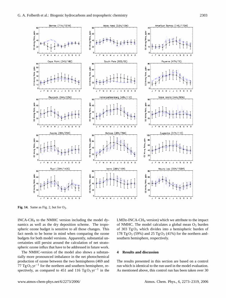
G. A. Folberth et al.: Biogenic hydrocarbons and tropospheric chemistry 2303
Fig. 14. Same as Fig.2, but for O3.
INCA-CH4 to the NMHC version including the model dy-namics as well as the dry deposition scheme. The tropo-spheric ozone budget is sensitive to all those changes. Thisfact needs to be borne in mind when comparing the ozonebudgets for both model versions. Apparently, substantial un-certainties still persist around the calculation of net strato-spheric ozone influx that have to be addressed in future work.
The NMHC-version of the model also shows a substan-tially more pronounced imbalance in the net photochemicalproduction of ozone between the two hemispheres (469 and77 Tg O3 yr−1 for the northern and southern hemisphere, re-spectively, as compared to 451 and 116 Tg O3 yr−1 in the
LMDz-INCA-CH4 version) which we attribute to the impactof NMHC. The model calculates a global mean O3 burdenof 303 Tg O3 which divides into a hemispheric burden of178 Tg O3 (59%) and 25 Tg O3 (41%) for the northern and-southern hemisphere, respectively.
4 Results and discussion
The results presented in this section are based on a controlrun which is identical to the run used in the model evaluation.As mentioned above, this control run has been taken over 30
www.atmos-chem-phys.net/6/2273/2006/ Atmos. Chem. Phys., 6, 2273–2319, 2006

2304 G. A. Folberth et al.: Biogenic hydrocarbons and tropospheric chemistry
Fig. 15. Measured (solid circles) and calculated (solid light blues lines indicate day-to-day variations, open diamonds denote monthly meanvalues) seasonal cycle of O3 mixing ratios (ppbv) at 7 stations and at the 800, 500, and 300 hPa levels. Observations were compiled byLogan(1999).
Atmos. Chem. Phys., 6, 2273–2319, 2006 www.atmos-chem-phys.net/6/2273/2006/

G. A. Folberth et al.: Biogenic hydrocarbons and tropospheric chemistry 2305
model months including a six months spin-up. The last 12months have been used in the analysis. In addition, we con-ducted several model experiments to study various aspects ofthe impact of NMVOC on tropospheric chemical composi-tion and photochemistry. These experiments are focused onthe impact of biogenic NMVOC which have their predomi-nant or unique source in the terrestrial biosphere, such as forinstance isoprene or methanol.
To quantify the impact of these compounds, four exper-iments have been carried out assessing the impact of iso-prene, biogenic methanol and acetone, as well as terpenes.In these experiments the respective emissions were turnedoff separately and changes in key tropospheric species, suchas ozone, OH, NOx and PAN, and HOx have been analyzed.We note that non-linearities in photochemistry can somewhatbias the results of these sensitivity experiments affecting theoxidation capacity of the atmosphere, likely towards an in-crease in the reactivity (measured by the OH concentration)when turning off the emissions, because the highly reactivebiogenic VOC are a strong OH sink. To quantify the uncer-tainties associated with the above mentioned non-linearities,we have performed an additional experiment with isopreneemissions reduced to 90% of their standard magnitude andcompared the results to the “standard” experiment with zeroisoprene emissions. All experiments were initialized with theJuly restart files of the first year of the control run and thencontinued over 18 model months. The last 12 months wereused for comparison.
4.1 Impact of Isoprene
The major impact of isoprene on tropospheric photochem-istry and chemical composition lies in its role as an ozoneprecursor and in the formation of organic nitrates in thecourse of isoprene photooxidation.Poisson et al.(2000)have shown that organic nitrate formation in the course ofNMVOC oxidation is responsible only for a minor decreaseof a few percent in NOx concentrations over polluted regions.The impact of NMVOC oxidation via the formation of PANand analogues significantly increases NOx concentrations inremote environments with only feeble NOx emissions, suchas the marine PBL. Thermal decomposition of PAN can in-crease NOx concentrations by almost a factor of 2, which isenough to significantly impact ozone and OH formation inthese remote areas.
During the northern hemispheric winter isoprene emis-sions are located predominantly at southern hemispherictropical latitudes. Emission rates reach maximum values of60 to 70×10−11 kg m−2 s−1 over the Amazon and Kongorain forest areas. At the same time, the NOx emissions occurprimarily at northern continental midlatitudes, where emis-sion fluxes can reach up to 18×10−11 kg m−2 s−1 over theEastern United States and Europe. A significant NOx sourceof approximately 6×10⁻¹¹ kg m−2 s−1 appears over equato-rial Africa which derives from a pronounced soil source dur-
ing the wet season in this region. In July the tropical isoprenesources have shifted toward the northern hemisphere. In ad-dition, a large new sources appears over the entire northernhemispheric continental midlatitudes. Here emission ratesare as high as 60×10−11 kg m−2 s−1 over the Eastern UnitedStates and Europe. On the other hand, the global distributionand magnitude of NOx surface sources has not changed muchwith the only exception of the NO-soil source over equatorialAfrica that is no longer present at this time of the year.
As a consequence, the global isoprene and NOx surfacesources appear to be separated in January during the north-ern hemispheric winter months. Half a year later, in July,these two sources coincide in many regions at northern hemi-spheric continental midlatitudes. This seasonally drivenswitch between separation and coincidence of NOx and iso-prene sources has important consequences for the chemistryof the lower troposphere. In January, isoprene oxidationlargely proceeds under NOx-limited conditions at southernlow- and midlatitudes with only a weak, biogenically drivenozone formation potential in the PBL. For these regions andtime of year the isoprene model experiment shows an in-crease in the ozone concentration at the surface of less than8 ppbv as depicted in the upper left map in Fig.16. More-over, the most pronounced increase occurs close to the NOsoil source over equatorial Africa. By contrast, the coincid-ing NOx and isoprene surface sources in July clearly holda strong ozone formation potential. This is reflected in theresults of the isoprene experiment by a strong increase ofozone directly over the source regions of up to 30 ppbv overthe Eastern United States and up to 20 ppbv over Europe asshown in the upper right map in Fig.16. This positive andhighly effective feedback between primarily anthropogenicNOx and entirely biogenic isoprene surface sources duringsummertime frequently leads to high-ozone episodes with re-lated air quality problems.
Furthermore, the changes in the ozone burden of the tro-posphere due to this coincidence-effect in particular and thebiogenic isoprene source in general potentially could affectthe radiative budget and, hence, contribute to climate change.To quantify the magnitude of the ozone net radiative forcingas a result of increased ozone levels we performed an offlineradiative transfer calculation using the ozone fields providedby the control run and the isoprene experiment. This calcula-tion predicts a global mean net radiative forcing of ozone dueto isoprene emissions of 0.09 W m−2. The ozone net radia-tive forcing is most pronounced at tropical latitudes rangingbetween 0.07 and 0.15 W m−2. Maximum values of up to0.17 W m−2 are found over the desert regions of northernAfrica and the Arabic Peninsula. At mid- and high latitudesof both hemispheres the O3 net radiative forcing ranges be-tween 0.02 and 0.09 W m−2.
Isoprene photooxidation is a significant source of carbonmonoxide. As shown in the lower two panels of Fig.16,isoprene oxidation near the surface results in an increase ofcarbon monoxide mixing ratios ranging from 25 to 60 ppbv
www.atmos-chem-phys.net/6/2273/2006/ Atmos. Chem. Phys., 6, 2273–2319, 2006
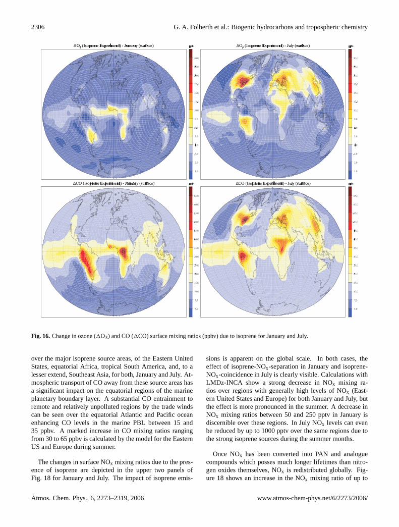
2306 G. A. Folberth et al.: Biogenic hydrocarbons and tropospheric chemistry
∆ ∆
∆ ∆
Fig. 16. Change in ozone (1O3) and CO (1CO) surface mixing ratios (ppbv) due to isoprene for January and July.
over the major isoprene source areas, of the Eastern UnitedStates, equatorial Africa, tropical South America, and, to alesser extend, Southeast Asia, for both, January and July. At-mospheric transport of CO away from these source areas hasa significant impact on the equatorial regions of the marineplanetary boundary layer. A substantial CO entrainment toremote and relatively unpolluted regions by the trade windscan be seen over the equatorial Atlantic and Pacific oceanenhancing CO levels in the marine PBL between 15 and35 ppbv. A marked increase in CO mixing ratios rangingfrom 30 to 65 ppbv is calculated by the model for the EasternUS and Europe during summer.
The changes in surface NOx mixing ratios due to the pres-ence of isoprene are depicted in the upper two panels ofFig. 18 for January and July. The impact of isoprene emis-
sions is apparent on the global scale. In both cases, theeffect of isoprene-NOx-separation in January and isoprene-NOx-coincidence in July is clearly visible. Calculations withLMDz-INCA show a strong decrease in NOx mixing ra-tios over regions with generally high levels of NOx (East-ern United States and Europe) for both January and July, butthe effect is more pronounced in the summer. A decrease inNOx mixing ratios between 50 and 250 pptv in January isdiscernible over these regions. In July NOx levels can evenbe reduced by up to 1000 pptv over the same regions due tothe strong isoprene sources during the summer months.
Once NOx has been converted into PAN and analoguecompounds which posses much longer lifetimes than nitro-gen oxides themselves, NOx is redistributed globally. Fig-ure 18 shows an increase in the NOx mixing ratio of up to
Atmos. Chem. Phys., 6, 2273–2319, 2006 www.atmos-chem-phys.net/6/2273/2006/

G. A. Folberth et al.: Biogenic hydrocarbons and tropospheric chemistry 2307
Fig. 17. Calculated annually and zonally averaged changes in O3 (ppbv), CH2O (ppbv), OH (%), and HOx (%) due to isoprene biogenicsurface emissions (412 Tg C yr−1).
50 pptv in January over the tropical oceans in the vicinity ofthe western continental regions. In July LMDz-INCA cal-culations seem to indicate that NOx is preferably releasedcloser to the regions with high levels of nitrogen oxides, inparticular over the northern hemispheric continental areas.This seems to be a consequence of the the shorter PAN life-times during the northern hemispheric summer months.
The lower two panels in Fig.18show the increase in PANmixing ratios at the surface for the isoprene experiment forJanuary and July. During the northern hemispheric wintera homogeneous increase in PAN over the entire extratropi-cal northern hemisphere ranging from 10 to 50 pptv is cal-culated by LMDz-INCA. This ubiquitous enhancement is aconsequence of the longer PAN lifetimes during the winterwhen thermal decomposition is less effective. The increase
in PAN in January is particularly strong close to the primaryisoprene sources of equatorial Africa, tropical South Amer-ica, and Southeast Asia. Over these regions the presence ofisoprene enhances PAN mixing ratios by up to 250 pptv.
In July the region of strong enhancements in the PAN sur-face mixing ratios is shifted to the northern hemispheric mid-latitudes. An increase in PAN between 75 and 750 pptv isdiscernible over most of the United States, Europe, and ex-tratropical Southeast Asia as a consequence of the isoprene-NOx-coincidence. This pronounced increase in PAN mixingratios is even more remarkable since PAN lifetimes are sig-nificantly shorter during the northern hemispheric summermonths. A homogeneous enhancement in PAN mixing ratios,albeit somewhat less pronounced, is apparent over southernhemispheric mid- to high latitudes in July, similar to the PAN
www.atmos-chem-phys.net/6/2273/2006/ Atmos. Chem. Phys., 6, 2273–2319, 2006

2308 G. A. Folberth et al.: Biogenic hydrocarbons and tropospheric chemistry
∆ ∆
∆ ∆
Fig. 18. Change in NOx (1NOx) and PAN (1PAN) surface mixing ratios (pptv) due to isoprene for January and July.
increase during northern hemispheric winter months. Thedevelopment of this extratropical “PAN plume” during thesouthern hemispheric winter owes its existence to the sameextension in PAN lifetimes but it is less distinctive due to sig-nificantly lower NOx sources in the Southern Hemisphere.The increase in PAN mixing ratios in the tropics is less pro-nounced in July as well reaching a surplus of up to 100 pptvover the tropical regions of South America and Africa.
The major sink of non-methane VOC in the troposphereis the reaction with hydroxyl radicals. As a result it is ex-pected that NMVOC have a significant impact on the globaldistribution of OH and, hence, the tropospheric oxidizing ca-pacity. Isoprene, and all other NMVOC that are emitted insignificant amounts, will compete for the OH radical.
Figure 17 shows the impact of global biogenic isopreneemissions on the ozone, formaldehyde, OH, and HOx distri-
bution and magnitude. LMDz-INCA calculates a reductionin the OH concentration reaching 50% near the surface overthe tropics and northern hemispheric mid-latitudes whereisoprene emissions are strongest. A decrease in OH rangingbetween 5% and 25% is also apparent in the free troposphereover the tropical and northern hemispheric mid- and high lat-itudes. In addition, the model calculates an isoprene inducedreduction of the global mean tropospheric OH concentrationby approximately 0.7×10⁵ molecules cm−3 or roughly 8%.This reduction in OH is most likely caused by isoprene pho-tooxidation products such as methacrolein and formaldehydewhich posses a substantially longer photochemical lifetimethan isoprene.
On the other hand, Formaldehyde and methacrolein life-times are too short for those species to be homogeneouslymixed in the troposphere. These two products of isoprene ox-
Atmos. Chem. Phys., 6, 2273–2319, 2006 www.atmos-chem-phys.net/6/2273/2006/

G. A. Folberth et al.: Biogenic hydrocarbons and tropospheric chemistry 2309
idation are displaced predominantly to the upper troposphereby deep convection in the tropics where they contribute sig-nificantly to the HOx budget of the UTLS region. Figure17shows that whereas the isoprene source reduces OH in mostof the troposphere its photochemical decomposition signif-icantly adds to the HOx concentration. This contributionis most pronounced in the tropical UTLS region where themodel calculates an increase in HOx between 10% and 20%.The additional HOx source is provided by photolysis of oxi-dation products such as for instance formaldehyde. Figure17depicts a corresponding increase of CH2O in the tropics onaccount of isoprene oxidation. Furthermore, it can be seenfrom Fig. 17 that isoprene oxidation yields an increase inHOx by more than 2.5% over the entire free and upper tropo-spher which translates into and increase of ozone concentra-tions between 2 and 5 ppbv.
Another important consequence of a reduced oxidative ca-pacity of the troposphere is the change in the lifetime ofmethane. The CH4 tropospheric lifetime is predominantlydetermined by its most important sink, the reaction with hy-droxyl radicals. Calculations with LMDz-INCA indicate anincrease in the global annual mean methane lifetime aver-aged over the entire tropospheric domain by approximately 7months or 6.5% as a consequence of global biogenic isopreneemissions.
The major products of isoprene photooxidation are methylvinyl ketone (MVK), methacrolein (MACR), and formalde-hyde (cf., e.g.,Sprengnether et al., 2002, and referencestherein). As discussed in detail byApel et al. (2002) thereaction of isoprene with OH favours the production ofMVK over MACR (MVK/MACR ≈1.4) whereas the reactionwith ozone produces MACR more abundantly than MVK(MVK/MACR ≈0.4). In our mechanism these ratios aresomewhat different (for a detailed discussion of differencesin current condensed isoprene oxidation mechanisms andtheir impact on global 3-D chemistry modelling see, e.g.,von Kuhlmann et al.(2004)): Under NOx-rich conditionsthe production ratio of MVK to MACR following the reac-tion of isoprene with OH is 0.9. This can become as lowas 0.6 under NOx-depleted conditions. In these NOx lim-ited environments the predominant products of the isoprene-OH reaction pathway are organic peroxides (Miyoshi et al.,1994) with increased methacrolein yields due to peroxiderecycling. The reaction of isoprene with ozone producesa MVK/MACR ratio even more biased toward productionof MACR with ratios reduced to approximately 0.4 in ourmodel. On the other hand, methyl vinyl ketone has a sig-nificantly longer photochemical lifetime than methacrolein.Hence, close to the isoprene sources at the surface the 0.9contour of the [MVK]/[MACR] ratio would indicate the tran-sition from NOx-rich to NOx-depleted areas.
Furthermore, due to the short photochemical lifetime ofisoprene of only a few hours the [MVK]/[MACR] ratio re-flects the aging of the isoprene-MVK-MACR mixture yield-ing potentially higher MVK/MACR ratios away from the iso-
Fig. 19. Ratio of the monthly mean methyl vinyl ketone andmethacrolein surface mixing ratios, [MVK]/[MACR], for Jannuaryand July.
prene sources. At considerable distance from the initial loca-tion of production the difference in lifetime takes precedenceover the production ratio and the [MVK]/[MACR] concen-tration ratio will shift toward a value equal or greater thanone. It is on account of this aspect that the ratio of the oxida-tion products MVK and MACR holds information about thehistory of the isoprene oxidation process.
Figure19depicts the monthly mean [MVK]/[MACR] con-centration ratio at the surface for January and July as cal-culated by LMDz-INCA. The major isoprene source areasof tropical South America, Africa, and South-East Asia areclearly marked by a [MVK]/[MACR] ratio of less than 0.9for both January and July indicating areas of isoprene oxida-tion in low-NOx environments and possibly non-negligible
www.atmos-chem-phys.net/6/2273/2006/ Atmos. Chem. Phys., 6, 2273–2319, 2006

2310 G. A. Folberth et al.: Biogenic hydrocarbons and tropospheric chemistry
Fig. 20. Calculated annually and zonally averaged changes in O3 (ppbv), CH2O (ppbv), OH (%), and HOx (%) due to acetone biogenicsurface emissions (47 Tg C yr−1).
contributions to isoprene oxidation by ozone. On the otherhand, most of the isoprene emissions in the Eastern UnitedStates during the summer months coincide with an abun-dance of NOx. This is reflected in the lower panel of Fig.19by [MVK]/[MACR] concentration ratios of 1.0 to 1.4 di-rectly over this region.
Large portions of the globe are characterized by[MVK]/[MACR] ratios between 1.1 and 1.2 which seem toindicate typical background conditions in regions that arestill under a direct influence of continental biogenic NMVOCemissions. Outside these regions, at high northern latitudes(northward of about 60◦ N) and in southern mid- and highlatitudes the concept of [MVK]/[MACR] concentration ra-tios as an indicator for the chemical history of air seemsto break down on account of the vanishing concentration of
both methylvinyl ketone and methacrolein. We refrain fromfurther speculating about these regions.
It is important, though, to emphasize that large uncertain-ties exists around the photochemistry of isoprene, and thephotochemistry of most organic compounds of biogenic ori-gin in general, as well as their representation in global 3-Dmodels of atmospheric chemistry. These uncertainties are re-lated not only to uncertainties in the global isoprene sourcedistribution and magnitude but also to the lack of detailedknowledge of all the chemical processes involved in thephotochemical decomposition of isoprene. Recently, effortshave been undertaken to quantify some of these uncertain-ties and their impact on modelling the chemical compositionof the atmosphere (e.g.Poschl et al., 2000; von Kuhlmannet al., 2004). Uncertainties with the most pronounced impact
Atmos. Chem. Phys., 6, 2273–2319, 2006 www.atmos-chem-phys.net/6/2273/2006/
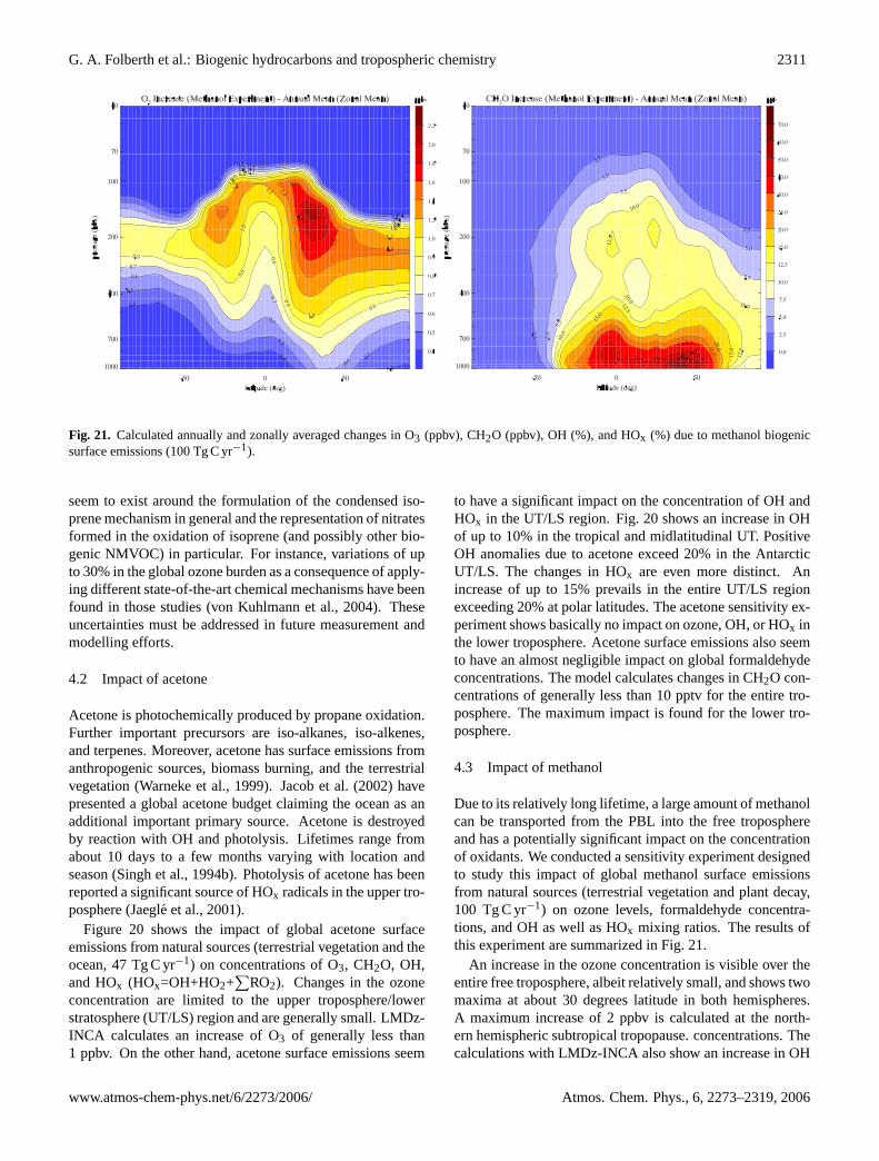
G. A. Folberth et al.: Biogenic hydrocarbons and tropospheric chemistry 2311
Fig. 21. Calculated annually and zonally averaged changes in O3 (ppbv), CH2O (ppbv), OH (%), and HOx (%) due to methanol biogenicsurface emissions (100 Tg C yr−1).
seem to exist around the formulation of the condensed iso-prene mechanism in general and the representation of nitratesformed in the oxidation of isoprene (and possibly other bio-genic NMVOC) in particular. For instance, variations of upto 30% in the global ozone burden as a consequence of apply-ing different state-of-the-art chemical mechanisms have beenfound in those studies (von Kuhlmann et al., 2004). Theseuncertainties must be addressed in future measurement andmodelling efforts.
4.2 Impact of acetone
Acetone is photochemically produced by propane oxidation.Further important precursors are iso-alkanes, iso-alkenes,and terpenes. Moreover, acetone has surface emissions fromanthropogenic sources, biomass burning, and the terrestrialvegetation (Warneke et al., 1999). Jacob et al.(2002) havepresented a global acetone budget claiming the ocean as anadditional important primary source. Acetone is destroyedby reaction with OH and photolysis. Lifetimes range fromabout 10 days to a few months varying with location andseason (Singh et al., 1994b). Photolysis of acetone has beenreported a significant source of HOx radicals in the upper tro-posphere (Jaegle et al., 2001).
Figure 20 shows the impact of global acetone surfaceemissions from natural sources (terrestrial vegetation and theocean, 47 Tg C yr−1) on concentrations of O3, CH2O, OH,and HOx (HOx=OH+HO2+
∑RO2). Changes in the ozone
concentration are limited to the upper troposphere/lowerstratosphere (UT/LS) region and are generally small. LMDz-INCA calculates an increase of O3 of generally less than1 ppbv. On the other hand, acetone surface emissions seem
to have a significant impact on the concentration of OH andHOx in the UT/LS region. Fig.20 shows an increase in OHof up to 10% in the tropical and midlatitudinal UT. PositiveOH anomalies due to acetone exceed 20% in the AntarcticUT/LS. The changes in HOx are even more distinct. Anincrease of up to 15% prevails in the entire UT/LS regionexceeding 20% at polar latitudes. The acetone sensitivity ex-periment shows basically no impact on ozone, OH, or HOx inthe lower troposphere. Acetone surface emissions also seemto have an almost negligible impact on global formaldehydeconcentrations. The model calculates changes in CH2O con-centrations of generally less than 10 pptv for the entire tro-posphere. The maximum impact is found for the lower tro-posphere.
4.3 Impact of methanol
Due to its relatively long lifetime, a large amount of methanolcan be transported from the PBL into the free troposphereand has a potentially significant impact on the concentrationof oxidants. We conducted a sensitivity experiment designedto study this impact of global methanol surface emissionsfrom natural sources (terrestrial vegetation and plant decay,100 Tg C yr−1) on ozone levels, formaldehyde concentra-tions, and OH as well as HOx mixing ratios. The results ofthis experiment are summarized in Fig.21.
An increase in the ozone concentration is visible over theentire free troposphere, albeit relatively small, and shows twomaxima at about 30 degrees latitude in both hemispheres.A maximum increase of 2 ppbv is calculated at the north-ern hemispheric subtropical tropopause. concentrations. Thecalculations with LMDz-INCA also show an increase in OH
www.atmos-chem-phys.net/6/2273/2006/ Atmos. Chem. Phys., 6, 2273–2319, 2006

2312 G. A. Folberth et al.: Biogenic hydrocarbons and tropospheric chemistry
on the order of one to two percent only. On the other hand,these calculations predict enhancements in the level of per-oxy radicals, such as HO2 and organic peroxy radicals, com-bined to HOx, between 8 and 15% in the UT/LS region de-pending on latitude. The increased supply of peroxy radicalsseems to drive the changes in ozone mixing ratios. The largeincrease in HOx in the UT/LS region could also be a conse-quence of CH2O photolysis. LMDz-INCA calculates a pro-nounced increase of formaldehyde in the lower tropospherebetween 50◦ S and 50◦N up to about 700 hPa with maximumpositive anomalies of 70 pptv in the PBL at about 40◦ N.At these altitudes formaldehyde photolysis is relatively weakand consequently CH2O lifetimes will be longer. The im-pact of methanol emissions on formaldehyde levels decreaseswith increasing altitude. The highly efficient destruction offormaldehyde by photolysis seems to be the reason for thevery small impact of methanol in the upper troposphere.
4.4 Global carbon monoxide budget for the troposphere
LMDz-INCA includes a set of tagged model tracers per-taining to the conversion of primary emitted VOC and in-termediate products of tropospheric photooxidation to car-bon monoxide and CO2 (Folberth et al., 2005). Using thesetagged tracers we present an updated estimate of the globalCO budget and compare our results to the estimates givenby Bergamaschi et al.(2000). Tab.8 summarizes both stud-ies. Note that our estimates are based on the assumptionthat global sources and sinks are in perfect equilibrium. Inparticular, this pertains to the tropospheric-stratospheric ex-change of CO which has been derived as the residual of allother sources and sinks calculated directly with the model.It should be pointed out as well that we have not attemptedto calculate uncertainty limits for our CO budget. Uncertain-ties in the global CO source are expected to be high and willdepend primarily on the uncertainties in the global emissioninventory. The uncertainties in the global sink are a conse-quence of the source uncertainties and are also expected tobe substantial.
Whereas the range of CO sources and sinks for individ-ual tropospheric processes in the study byBergamaschi et al.(2000) represent a posteriori estimates obtained by an in-verse modelling approach, the current CO budget has beenderived with a forward model. Furthermore, the studies arebased on fundamentally different emission inventories. Nev-ertheless, both modelling studies agree surprisingly well intheir predictions of the total global CO sources and sinks.Note that in the LMDz-INCA standard emission inventory(cf. Table5) CO emissions deriving from agricultural wasteburning and domestic biofuel use have been attributed to theglobal biomass burning source. In the study ofBergamaschiet al. (2000) these sources are included in the technologicalsource category. For the purpose of this comparison we lim-ited the CO biomass burning source to savannah and forestfires only attributing carbon monoxide emissions from agri-
cultural waste burning and domestic biofuel use to the tech-nological sources. With these changes in categories, the car-bon monoxide budget calculated by LMDz-INCA and sum-marized in Table8 appears to be in very good agreement withthe study ofBergamaschi et al.(2000).
Secondary CO sources in LMDz-INCA deriving from re-active carbon compound (RCC) photooxidation in the tropo-sphere amount to 1489 Tg CO yr−1. RCC include all carboncontaining compounds that are chemically broken down inthe troposphere, excluding only CO2 which is chemically in-ert. Oxidation of methane, isoprene, methanol, terpenes, ace-tone, and other non-methane VOC (mostly of anthropogenicorigin), respectively, contribute 854, 359, 110, 49, 28, and89 Tg CO yr−1 to this secondary carbon monoxide source. Ingeneral, conversion efficiencies – defined as the ratio of theamount of carbon emitted in the form of individual speciesto the amount of carbon converted to CO expressed in per-cent – are less than 50% (20%–45%) for all species otherthan methane and CO. Therefore, it follows that these speciesmust posses other highly efficient sinks. These sinks arefound to be the physical removal of primary emitted VOCas well as their stable intermediate photochemical products(such as alcohols, aldehydes, ketones, and organic nitrates)through surface dry deposition and wet removal. The CH4conversion efficiency of 90% indicates that photochemicaldestruction is by far the most important atmospheric sink,CH4 entrainment to the stratosphere being the only other sig-nificant removal process in our model. It has been shown,however, that dry deposition of methane at the surface due tosoil-microbial activity amounts to approximately 30 TgCH4(cf. Prather et al.(2001)) and is roughly of equal importanceas stratospheric destruction. For lack of a parameterization ofthis process suitable for global chemistry-climate models wedecided to neglect methane dry deposition in LMDz-INCAat this stage.
Both studies agree closely on the global CO sink. Pho-tochemical oxidation of carbon monoxide, which representsa significant secondary CO2 source (Folberth et al., 2005),constitutes a slightly stronger sink in LMDz-INCA. Calcu-lations with LMDz-INCA indicate a global CO-to-CO2 con-version efficiency of 88%. On the other hand, dry deposi-tion of CO at the surface seems to be significantly weaker inLMDz-INCA than in the study ofBergamaschi et al.(2000).The residual of all sources and sinks of carbon monoxide inour model is interpreted as a CO entrainment to the strato-sphere. The estimate of this particular sink significantly ex-ceeds the estimate ofBergamaschi et al.(2000) as a conse-quence of the substantially weaker CO surface deposition.
5 Summary and conclusions
In this paper we provide a first description and evaluation ofa new version of the 3-D-chemistry-climate model LMDz-INCA. This new version is based on the recently devel-
Atmos. Chem. Phys., 6, 2273–2319, 2006 www.atmos-chem-phys.net/6/2273/2006/

G. A. Folberth et al.: Biogenic hydrocarbons and tropospheric chemistry 2313
oped CH4-NOx-CO-O3 version of LMDz-INCA to which acomprehensive representation of the photochemistry of non-methane hydrocarbons (NMHC) and volatile organic com-pounds (VOC) has been added. The current version runs witha horizontal resolution of 3.8×2.5 degrees in longitude andlatitude, respectively, and the vertical model domain extendsover 19 levels from the surface up to 3 hPa. The model cal-culates the distribution of tropospheric ozone and its precur-sors as well as a substantial number of primary NMVOC andintermediate photochemical products, such as isoprene, ace-tone, methanol, PAN and analogues, or formaldehyde. Sur-face emissions are based on state-of-the-art emission inven-tories. Biogenic VOC emissions from the terrestrial vege-tation are calculated with the dynamic vegetation and emis-sion model ORCHIDEE and are provided off-line to LMDz-INCA. The model is run in climatological mode and the re-sults are evaluated by thorough comparison with observa-tions inasmuch as they are available.
The model captures well the distribution and seasonal cy-cle of carbon monoxide except for a tendency to overesti-mate CO by up to 20 ppb at southern mid and high lati-tudes. The tropospheric annual mean methane (9.2 years)and methylchloroform (5.5 years) chemical lifetimes are inexcellent agreement with estimates obtained by observa-tions indicating that LMDz-INCA simulates the global tro-pospheric OH distribution and magnitude (annual mean OHabundance of 9.6×10⁵ molecules cm−3) fairly well. A com-parison with observed vertical profiles of NOx, PAN, andHNO3 indicate that LMDz-INCA is capable of well repro-ducing the distribution of nitrogen compounds, even thoughthe problem of overestimated nitric acid concentrations, pre-vailing in many current chemistry models, also persists inLMDz-INCA, albeit to a somewhat reduced extent.
The model also satisfactorily simulates a variety ofnon-methane volatile organic compounds, such as acetone,methanol, and formaldehyde. The comparison with observa-tions reveal a generally good agreement for these species.Locally, however, methanol can be underestimated by upto a factor of 2.5 at some remote locations. The compar-ison also indicates that the model overestimates measuredformaldehyde concentrations in the lower and middle tropo-sphere over the South Atlantic by up to a factor of three.This disagreement could be related to an overestimate offormaldehyde or its precursors from biomass burning beingtoo high in our emission inventory near this region (SouthAmerican continental sources). The comparison of acetoneprofiles with observations show a fairly well model-to-dataagreement over the entire troposphere.
The model reproduces fairly well the magnitude and distri-bution of ozone in the entire troposphere. Annual mean tro-pospheric photochemical production (4436 Tg O3 yr−1), anddestruction (3890 Tg O3 yr−1), dry deposition at the surface(1261 Tg O3 yr−1), and stratospheric influx (715 Tg O3 yr−1)are in good agreement with analogue estimates of currentphotochemical models. A net tropospheric ozone production
Table 8. Carbon monoxide budget for the global troposphere de-fined as the region extending from the surface up to the 250 hPaaltitude level. LMDz-INCA results are compared to the a posteri-ori estimates obtained by an inverse modelling study of the globalCO cycle as given byBergamaschi et al.(2000). All numbers arewritten as Tg CO yr−1. The average and range (in brackets) of esti-mates for the study of Bergamaschi et al. is denoted. Percent valuesin parentheses indicate VOC-to-CO conversion efficiencies calcu-lated with the LMDz-INCA model.
LMDz-INCA Bergamaschi et al.(2000)
Global Source 3019 2818 (2244–3392)Primary Source 1533 1349 (1022–1675)Biomass Burning 811 674 (506–840)Technological 672 656 (511–800)Oceanic 50 19 (5–35)RCCa Oxidation 1489 (55%) 1468 (1220–1715)Methaneb 854 (90%) 831Isoprene 359 (37%) 348 (231–464)Methanol 110 (45%) —Terpenes 49 (22%) 145 (98–191)Acetone 28 (24%) —∑
other VOCc 89 (38%) 145 (61–229)
Global Sink 3019 2938 (2863–3010)PhotochemicalDestruction 2653 2471 (2415–2529)Dry Deposition 135 301 (292–308)StratosphericEntrainment 231 166 (156–173)
a reactive carbon compounds (cf. text for definition)b fixed inBergamaschi et al.(2000); calculated in LMDz-INCAc mostly anthropogenic
rate of 546 Tg O3 yr−1 is calculated by LMDz-INCA whichis about 75% of the the stratospheric influx.
The new version of LMDz-INCA has been applied tostudy the impact of isoprene (411 Tg C yr−1), acetone(50 Tg C yr−1), and methanol (104 Tg C yr−1) surface emis-sions on ozone and other tropospheric oxidants. Isopreneemissions are found to have a substantial impact on ozoneand carbon monoxide concentrations. The isoprene experi-ment also shows a separation of NOx and isoprene sourcesin January and an isoprene-NOx-coincidence in July witha low and high ozone formation potential in January andJuly, respectively. The calculations with LMDz-INCA showa strong increase of up to 30 ppbv at the surface over theEastern United States and Europe in the summer as a con-sequence of the coincidence of NOx and isoprene surfacesources. To assess the potential importance of these changesin the tropospheric ozone burden on the radiative budgetof the atmosphere, an offline radiative calculation has beenconducted. A global mean ozone net radiative forcing of0.09 W m−2 is calculated with maximum values reaching
www.atmos-chem-phys.net/6/2273/2006/ Atmos. Chem. Phys., 6, 2273–2319, 2006

2314 G. A. Folberth et al.: Biogenic hydrocarbons and tropospheric chemistry
0.17 W m−2 at tropical latitudes. The radiative effect of anincreasing ozone burden in the troposphere as a result ofbiogenic isoprene surface emissions on the atmospheric ra-diative budget, therefore, appears to be non-negligible butrather small as compared to other seemingly more importanteffects. However, an increase in the source of troposphericozone precursors, such as NOx and BVOC originating froma more active biosphere, as a consequence of a changing cli-mate (c.f., e.g.,Lathiere et al., 2005a; Hauglustaine et al.,2005), could potentially represent a positive feedback pro-cess enhancing global warming. Clearly, a more detailed in-vestigation is needed.
Compared with a non-isoprene run, carbon monoxide mix-ing ratios are found to increase between 25 and 60 ppbvover continental isoprene source regions and between 15and 30 ppb in the remote marine boundary layer. An im-portant role role of isoprene lies in its impact on the redis-tribution of nitrogen oxides in the entire troposphere dueto the conversion of short-lived NOx into organic nitrateswith significantly longer lifetimes. Photooxidation of iso-prene provides large amounts of organic nitrate precursors.An increase in PAN mixing ratios at the surface rangingfrom 10 to 250 pptv and 75 to 750 pptv during northernhemispheric winter and summer months, respectively, is cal-culated by LMDz-INCA. A decrease in the zonally aver-aged annual mean OH concentration ranging between 5%and 25% in the tropical and northern hemispheric free tro-posphere is calculated by our model as a consequence of theglobal biogenic isoprene source. An isoprene induced reduc-tion of the tropospheric OH concentration by approximately0.7×105 molecules cm−3 or roughly 8% is calculated on theglobal average. Ensuing this reduction in the oxidative ca-pacity the model predicts an increase of the global mean tro-pospheric methane lifetime by approximately seven months.At the same time the model shows an increase of the HOxconcentration in the entire free and upper troposphere dueto isoperene with a maximum value of 20% for the tropicalUTLS region. Our simulations reveal [MVK]/[MACR] ratiosof less than 0.9 over NOx depleted isoprene source regionsfor both January and July whereas a [MVK]/[MACR] ratio ofup to 1.4 is calculated over the Eastern United States in Julywhere pronounced isoprene emissions coincide with a highNOx burden. It has to be kept in mind, though, that the treat-ment of isoprene photochemistry in current global chemistrymodels is still associated with large uncertainties pertainingto its sources and representation of the chemistry. These un-certainties must be reduced in future measurement and mod-elling efforts because the photochemistry of isoprene and itsoxidation products represents a key component in the under-standing of tropospheric photochemistry.
Acetone and methanol play a significant role in controllingtropospheric oxidants in the upper troposphere/lower strato-sphere region. The sensitivity experiments show a smallimpact of global acetone surface emissions on troposphericozone but indicate a strong impact on the OH and peroxy
radical budget of the UT/LS region. An increase between10% and 15% in the UT/LS in the OH and HOx concentra-tion is calculated by the model. Interestingly, acetone seemsto have the most pronounced impact over the polar regions,at least when measured as percent changes. In case of themethanol sensitivity experiments, calculations show maxi-mum positive anomalies of 2 ppbv for ozone, 2% for OH, and8 to 15% for HOx, respectively. Both species show relativelysmall impacts on tropospheric formaldehyde concentrationswith maximum changes of 10 pptv and 70 pptv for acetoneand methanol, respectively. Both these maxima occur in thelower troposphere or even in the PBL.
We also attempted an estimate of the CO budget for theglobal troposphere and compared the results to a recentlypublished inverse modelling study. Even though our studyand the study byBergamaschi et al.(2000) have used fun-damentally different approaches to derive their estimates ofglobal tropospheric CO sources and sinks (a forward cal-culation in LMDz-INCA versus a posteriori estimates ob-tained by means of an inverse modelling approach in thestudy Bergamaschi et al.) both studies show a strikinglysimilar global picture. A global carbon monoxide source of3019 Tg CO yr−1, which divides into a primary CO source of1533 Tg CO yr−1 originating from biomass burning, techno-logical, and oceanic sources and a secondary CO source of1489 Tg CO yr−1 due to methane and VOC photooxidation,is calculated by LMDz-INCA. Oxidation of methane, iso-prene, methanol, terpenes, acetone, and other non-methaneVOC, respectively, are found to contribute 854, 359, 110,49, 28, and 89 Tg CO yr−1 to this secondary CO source.The model calculates global VOC-to-CO conversion efficien-cies ranging from 20 to 45%, a 90% conversion efficiency isprognosticated in case of methane. Oxidation of CO rep-resents by far the most important tropospheric sink. Ac-cording to our calculations, 2653 Tg CO yr−1 are removedfrom the troposphere by this process indicating a global CO-to-CO2 conversion efficiency of 88%. Surface depositionof CO (135 Tg CO yr−1) and stratospheric CO entrainment(231 Tg CO yr−1) are identified as the only significant tropo-spheric carbon monoxide sinks other than CO oxidation.
In summary, the NMHC version of LMDz-INCA providesan overall satisfactory representation of the complex pho-tochemical processes of the tropospheric VOC compositionas well as the budgets of key tropospheric species such as,e.g., O3 and CO. The new version has been applied in sev-eral sensitivity studies addressing the interaction between thecontinental biosphere and atmospheric chemical composi-tion. Current development efforts are focused on halogenphotochemistry, an interactive climate-chemistry coupling,and integration of LMDz-INCA with the dynamic vegeta-tion and emission model ORCHIDEE providing a compre-hensive modelling tool to study more directly the numerousfeedbacks between the biosphere, the atmosphere, climate,and photochemistry. Results from these new versions will bereported in forthcoming studies.
Atmos. Chem. Phys., 6, 2273–2319, 2006 www.atmos-chem-phys.net/6/2273/2006/

G. A. Folberth et al.: Biogenic hydrocarbons and tropospheric chemistry 2315
Acknowledgements.This work was partly funded by the EuropeanCommission under contract EVK2-CT-2002-00170. GF acknowl-edges support provided by the Canadian Centre for Climate Mod-elling and Analysis. We would like to thank William J. Collins andan anonymous reviewer for their adjuvant comments which helpedto improve the manuscript significantly. Additional funding hasbeen received from the GCC project and support by NSERC andCFCAS is gratefully acknowledged. Computer resources were pro-vided by the Commissariata l’Energie Atomique under project p24.
Edited by: A. B. Guenther
References
Altshuller, A. P.: PANs in the atmosphere, J. Air & Waste Manage.Assoc., 43, 1221–1230, 1993.
Andreae, M.: Climatic effects of changing atmospheric aerosol lev-els, in: Future Cliamtes of the World, edited by: Henderson-Sellers, A., Vol. 16 of World Survey of Climatology, pp. 341–392, Elsvier, Amsterdam, 1995.
Andreae, M. and Crutzen, P.: Atmospheric aerosols: biogeochem-ical sources and role in atmospheric chemistry, Science, 276,1052–1058, 1997.
Andreae, M. O. and Merlet, P.: Emission of trace gases and aerosolsfrom biomass burning, Global Biogeochem. Cycles, 15, 955–966, 2001.
Apel, E. C., Riemer, D. D., Hills, A., Baugh, W., Orlando, J.,Faloona, I., Tan, D., Brune, W., Lamb, B., Westberg, H., Car-roll, M. A., Thornberry, T., and Geron, C. D.: Measurementand interpretation of isoprene fluxes and isoprene, methacrolein,and methyl vinyl ketone mixing ratios at the prophet site dur-ing the 1998 intensive, J. Geophys. Res.-Atmos., 107(D3), 4034,doi:10.1029/2000JD000225, 2002.
Atkinson, R., Baulch, D., Cox, R., Hampson, R., Kerr, J., Rossi, M.,and Troe, J.: Evaluated kinetic and photochemical data for atmo-spheric chemistry: Supplement v, J. Physi. Chem. Ref. Data, 26,1125–1568, 1997.
Balkanski, Y., Jacob, D., Gardner, G., Graustein, W., and Turekian,K.: Transport and residence times of tropospheric aerosols in-ferred from a global three-dimensional simulation of210Pb, J.Geophys. Res., 98, 20 573–20 586, 1993.
Barrie, L. A., Bottenheim, J. W., Schnell, R. C., Crutzen, P. J.,and Rasmussen, R. A.: Ozone destruction and photochemical-reactions at polar sunrise in the lower arctic atmosphere, Nature,334, 138–141, 1988.
Bauer, S. E., Balkanski, Y., Schulz, M., Hauglustaine, D. A., andDentener, F.: Global modeling of heterogeneous chemistry onmineral aerosol surfaces: Influence on tropospheric ozone chem-istry and comparison to observations, J. Geophys. Res.-Atmos.,109, D02304, doi:10.1029/2003JD003868, 2004.
Baulch, D., Cobos, C., Cox, R. A., Esser, C., Frank, P., Just, T.,Kerr, J., Pilling, M., Troe, J., Walker, R., and Warnatz, J.: Evalu-ated kinetic data for combustion modelling, J. Phys. Chem. Ref.Data, 21, 411–429, 1992.
Bergamaschi, P., Hein, R., Heimann, M., and Crutzen, P. J.: Inversemodeling of the global CO cycle 1. inversion of CO mixing ra-tios, J. Geophys. Res.-Atmos., 105, 1909–1927, 2000.
Bernard, S. M., Samet, J. M., Grambsch, A., Ebi, K. L., andRomieu, I.: The potential impacts of climate variability andchange on air pollution-related health effects in the united states,Environ. Health Perspect., 109, 199–209, 2001.
Berntsen, T. K., Isaksen, I. S. A., Myhre, G., Fuglestvedt, J. S.,Stordal, F., Larsen, T. A., Freckleton, R. S., and Shine, K. P.:Effects of anthropogenic emissions on tropospheric ozone and itsradiative forcing, J. Geophys. Res.-Atmos., 102, 28 101–28 126,1997.
Bey, I., Jacob, D. J., Yantosca, R. M., Logan, J. A., Field, B. D.,Fiore, A. M., Li, Q. B., Liu, H. G. Y., Mickley, L. J., and Schultz,M. G.: Global modeling of tropospheric chemistry with assim-ilated meteorology: Model description and evaluation, J. Geo-phys. Res.-Atmos., 106, 23 073–23 095, 2001.
Bonsang, B. and Boissard, C.: Global distribution of reactive hy-drocarbons in the atmosphere, in: Reactive Hydrocarbons in theAtmosphere, pp. 209–265, Academic Press, 1999.
Bonsang, B., Polle, C., and Lembert, G.: Evidence for marine pro-duction of isoprene, Geophys. Res. Lett., 19, 1129–1132, 1992.
Boucher, O., Pham, M., and Venkataraman, C.: Simulation of theatmospheric sulfur cycle in the laboratoire de meteorologie dy-namique general circulation model. Model description, modelevaluation, and global and european budgets, Note scientifiquede l’IPSL n. 23, 2002.
Bouwman, A. F. and Taylor, J. A.: Testing high-resolution nitrousoxide emission estimates against observations using an atmo-spheric transport model, Global Biogeochem. Cycles, 10, 307–318, 1996.
Bradley, J. N., Edwards, A. D., and Gilbert, J. R.: Gas-phase re-actions of singlet oxygen atoms with methane, Journal of theChemical Society a -Inorganic Physical Theoretical, p. 326pp.,1971.
Brasseur, G. and Chatfield, R.: The fate of biogenic trace gases inthe atmosphere, in: Trace Gas Emissions from Plants, edited by:Sharkey, T., Holland, E., and Mooney, H., pp. 1–27, AcademicPress, 1991.
Brasseur, G. and Solomon, S.: Aeronomy of the Middle Atmo-sphere: Chemistry and Physics of the Stratosphere and Meso-sphere, Atmospheric Science Library, D. Reidel Pub. Co., 2ndedn., 1987.
Brasseur, G., Orlando, J., and Tyndall, G.: Atmospheric Chemistryand Global Change, Oxford Univ. Press, New York, 1999.
Brasseur, G. P., Hauglustaine, D. A., Walters, S., Rasch, P. J.,Muller, J. F., Granier, C., and Tie, X. X.: Mozart, a globalchemical transport model for ozone and related chemical trac-ers 1. model description, J. Geophys. Res.-Atmos., 103, 28 265–28 289, 1998.
Brocheton, F.: Representation desemissions anthropogiquesdans les models globaux de chimie-transport: sensibilite a larepresentation spatiale desemissions et au degre de raffinementdu schema chimique, Ph.D., Universite Paris 12 – Val de Marne,1999.
Burden, R. and Faires, J.: Numerical Analysis, PWS, Boston,Mass., 1985.
Chang, J., Brost, R., Isaksen, I., Madronich, S., Middleton, P.,Stockwell, W., and Walcek, C.: A three-dimensional Eulerianacid deposition model: Physical concepts and formulation, J.Geophys. Res., 92, 14 681–14 700, 1987.
Collins, W. J., Derwent, R. G., Johnson, C. E., and Stevenson, D. S.:The oxidation of organic compounds in the troposphere and theirglobal warming potentials, Climatic Change, 52, 453–479, 2002.
Constable, J. V. H., Guenther, A. B., Schimel, D. S., and Monson,R. K.: Modelling changes in voc emission in response to climate
www.atmos-chem-phys.net/6/2273/2006/ Atmos. Chem. Phys., 6, 2273–2319, 2006
2316 G. A. Folberth et al.: Biogenic hydrocarbons and tropospheric chemistry
change in the continental united states, Global Change Biology,5, 791–806, 1999.
Corbett, J. J., Fischbeck, P. S., and Pandis, S. N., Global nitrogenand sulfur inventories for oceangoing ships, J. Geophys. Res.-Atmos., 104, 3457–3470, 1999.
Crutzen, P.: The role of NO and NO2 in the chemistry of the tro-posphere and stratosphere, Ann. Rev. Earth Planet. Sci., 7, 443–472, 1979.
Crutzen, P.: Ozone in the troposphere, in: Composition, Chemistry,and Climate of the Atmosphere, edited by: Singh, H., pp. 349–393, Van Nostrand Reinold, New York, 1995.
Crutzen, P. and Zimmermann, P.: The changing photochemistry ofthe troposphere, Tellus, 43, 136–151, 1991.
De Fries, R. and Townshend, J.: NDVI-derived land classificationat global scales, Int. J. Remote Sens., 15, 3567–3586, 1994.
de Rosnay, P. and Polcher, J.: Modelling root water uptake in acom-plex land surface scheme coupled to a gcm, Hydrol. Earth Syst.Sci., 2, 239–256, 1998.
DeMore, W., Sander, S., Golden, D., Hampson, R., Kurylo, M.,Howard, C., Ravishankara, A., Kolb, C., and Molina, M.: Chem-ical kinetics and photochemical data for use in stratospheric mod-eling, evaluation number 12, 1997.
Dlugokencky, E. J., Masarie, K. A., Lang, P. M., and Tans, P. P.:Continuing decline in the growth rate of the atmospheric methaneburden, Nature, 393, 447–450, 1998.
Doskey, P. and Gao, W.: Vertical mixing and chemistry of isoprenein the atmospheric boundary layer: Aircraft-based measurementsand numerical modeling, J. Geophys. Res., 104, 21 263–21 274,1999.
Ducoudre-De Noblet, N., Laval, K., and Perrier, A.: Sechiba, anew set of parametrizations of the hydrologic exchanges at theland/atmosphere interface within the lmd atmospheric generalcirculation model, J. Climate, 2, 248–273, 1993.
Dufresne, J. L., Friedlingstein, P., Berthelot, M., Bopp, L., Ciais,P., Fairhead, L., Le Treut, H., and Monfray, P.: On themagnitude of positive feedback between future climate changeand the carbon cycle, Geophys. Res. Lett., 29, 10, 1405,doi:10.1029/2001GL013777, 2002.
Emmons, L. K., Hauglustaine, D. A., Muller, J. F., Carroll, M. A.,Brasseur, G. P., Brunner, D., Staehelin, J., Thouret, V., andMarenco, A.: Data composites of airborne observations of tropo-spheric ozone and its precursors, J. Geophys. Res.-Atmos., 105,20 497–20 538, 2000.
Erickson, D. J. and Taylor, J. A.: 3-d tropospheric co modeling – thepossible influence of the ocean, Geophys. Res. Lett., 19, 1955–1958, 1992.
Fehsenfeld, F., Calvert, J., Fall, R., Goldan, P., Guenther, A., He-witt, C., Lamb, B., Liu, S., Trainer, M., Westberg, H., and Zim-merman, P.: Emissions of volatile organic compounds from veg-etation and the implications for atmospheric chemistry, GlobalBiogeochem. Cycles, 6, 389–430, 1992.
Finlaysonpitts, B. J. and Pitts, J. N.: Atmospheric chemistry of tro-pospheric ozone formation - scientific and regulatory implica-tions, J. Air & Waste Manage. Assoc., 43, 1091–1100, 1993.
Fishman, J.: The global consequences of increasing troposphericozone concentrations, Chemosphere, 22, 685–695, 1991.
Folberth, G., Hauglustaine, D. A., Ciais, P., and Lathiere, J.: On therole of atmospheric chemistry in the global CO2 budget, Geo-phys. Res. Lett., 32, L08801, doi:10.1029/2004GL021812, 2005.
Friedlingstein, P., Bopp, L., Ciais, P., Dufresne, J. L., Fairhead, L.,Le Treut, H., Monfray, P., and Orr, J.: Positive feedback betweenfuture climate change and the carbon cycle, Geophys. Res. Lett.,28, 1543–1546, 2001.
Fung, I., John, J., Lerner, J., Matthews, E., Prather, M., Steele, L.,and Fraser, P., Three-dimensional model synthesis of the globalmethane cycle, J. Geophys. Res.-Atmos., 96, 13 033–13 066,1991.
Galbally, I. E. and Kirstine, W.: The production of methanol byflowering plants and the global cycle of methanol, J. Atmos.Chem., 43, 195–229, 2002.
Ganzeveld, L. and Lelieveld, J.: Dry Deposition Parameterization ina Chemistry General-Circulation Model and Its Influence On theDistribution of Reactive Trace Gases, J. Geophys. Res.-Atmos.,100(D10), 20 999–21 012, 1995.
Ganzeveld, L. and Lelieveld, J., and Roelofs, G. J.: A dry depositionparameterization for sulfur oxides in a chemistry and general cir-culation model, J. Geophys. Res.-Atmos. , 103(D5) , 5679–5694,1998.
Gardner, R. et al., ANCAT/EC2 global aircraft emission inventoriesfor 1991/92 and 2015: Report by the ECAC/ANCAT and ECWorking Group, Tech. rep., Def. Eval. and Res. Agency, Farn-borough, UK, 1998.
Giorgi, F. and Chameides, W.: The rainout parameterization in aphotochemical model, J. Geophys. Res., 90, 7872–7880, 1985.
Graedel, T.: Terpenoids in the atmosphere, Rev. Geophys. SpacePhys., 17, 937–947, 1979.
Granier, C., Petron, G., Muller, J., and Brasseur, G.: The impactof natural and anthropogenic hydrocarbons on the troposphericbudget of carbon monoxide, Atmos. Environ., 34, 5255–5270,2000.
Greenberg, R. and Heicklen, J.: The reaction of O(1D) with CH4,Int. J. Chem. Kinet., 4, 471, 1972.
Guenther, A., Hewitt, C., Erickson, D., Fall, R., Geron, C., Graedel,T., Harley, P., Klinger, L., Lerdau, M., McKay, W., Pierce, T.,Scholes, B., Steinbrecher, R., Tallamraju, R., Taylor, J., and Zim-merman, P.: A global model of natural volatile organic com-pound emissions, J. Geophys. Res., 100, 8873–8892, 1995.
Guenther, A., Archer, S., Greenberg, J., Harley, P., Helmig,D., Klinger, L., Vierling, L., Wildermuth, M., Zimmerman,P., and Zitzer, S.: Biogenic hydrocarbon emissions and land-cover/climate change in a subtropical savanna, Phys. Chem.Earth Part B-Hydrol. Oceans Atmos., 24, 659–667, 1999.
Guenther, A., Geron, C., Pierce, T., Lamb, B., Harley, P., andFall, R.: Natural emissions of non-methane volatile organic com-pounds; carbon monoxide, and oxides of nitrogen from northamerica, Atmos. Environ., 34, 2205–2230, 2000.
Hall, I., Wayne, R. P., Cox, R. A., Jenkin, M., and Hayman, G.: Ki-netics of the reaction of NO3 with HO2, J. Phys. Chem., 92(17),5049–5054, 1988.
Hao, W. and Liu, M.: Spatial and temporal distribution of tropicalbiomass burning, Global Biogeochem. Cycles, 8, 495–503, 1994.
Harzallah, A. and Sadourny, R.: Internal versus sst-forced at-mospheric variability as simulated by an atmospheric general-circulation model, J. Climate, 8, 474–495, 1995.
Hauglustaine, D. A. and Brasseur, G. P.: Evolution of tropo-spheric ozone under anthropogenic activities and associated ra-diative forcing of climate, J. Geophys. Res.-Atmos., 106, 32 337–32 360, 2001.
Atmos. Chem. Phys., 6, 2273–2319, 2006 www.atmos-chem-phys.net/6/2273/2006/
G. A. Folberth et al.: Biogenic hydrocarbons and tropospheric chemistry 2317
Hauglustaine, D. A., Granier, C., Brasseur, G. P., and Megie, G.:The importance of atmospheric chemistry in the calculation of ra-diative forcing on the climate system, J. Geophys. Res.-Atmos.,99, 1173–1186, 1994.
Hauglustaine, D. A., Brasseur, G. P., Walters, S., Rasch, P. J.,Muller, J. F., Emmons, L. K., and Carroll, C. A.: Mozart, a globalchemical transport model for ozone and related chemical tracers2. model results and evaluation, J. Geophys. Res.-Atmos., 103,28 291–28 335, 1998.
Hauglustaine, D. A., Hourdin, F., Jourdain, L., Filiberti, M. A.,Walters, S., Lamarque, J. F., and Holland, E. A.: Interactivechemistry in the laboratoire de meteorologie dynamique gen-eral circulation model: Description and background troposphericchemistry evaluation, J. Geophys. Res.-Atmos., 109, D04314,doi:10.1029/2003JD003 957, 2004.
Hauglustaine, D. A., Lathiere, J., Szopa, S., and Folberth,G. A.: Future tropospheric ozone simulated with a climate-chemistry-biosphere model, Geophys. Res. Lett., 32, L24807,doi:10.1029/2005GL024031, 2005.
Heikes, B. G., Chang, W. N., Pilson, M. E. Q., Swift, E., Singh,H. B., Guenther, A., Jacob, D. J., Field, B. D., Fall, R.,Riemer, D., and Brand, L.: Atmospheric methanol budget andocean implication, Global Biogeochem. Cycles, 16(4), 1133,doi:10.1029/2002GB001895, 2002.
Highwood, E. J., Shine, K. P., Hurley, M. D., and Wallington, T. J.:Estimation of direct radiative forcing due to non-methane hydro-carbons, Atmos. Environ., 33, 759–767, 1999.
Horowitz, L. W., Walters, S., Mauzerall, D. L., Emmons, L. K.,Rasch, P. J., Granier, C., Tie, X. X., Lamarque, J. F., Schultz,M. G., Tyndall, G. S., Orlando, J. J., and Brasseur, G. P.: A globalsimulation of tropospheric ozone and related tracers: Descriptionand evaluation of MOZART, version 2, J. Geophys. Res.-Atmos.,108(D24), 4784, doi:10.1029/2002JD002853, 2003.
Hourdin, F. and Armengaud, A.: The use of finite-volume meth-ods for atmospheric advection of trace species-1. test of variousformulations in a general circulation model, Mon. Wea. Rev.,127(5), 822–837, 1999.
Houweling, S., Dentener, F., and Lelieveld, J.: The impact of non-methane hydrocarbon compounds on tropospheric photochem-istry, J. Geophys. Res., 103, 10 673–10 696, 1998.
Jacob, D. J.: Heterogeneous chemistry and tropospheric ozone, At-mos. Environ., 34, 2131–2159, 2000.
Jacob, D. J., Field, B. D., Jin, E. M., Bey, I., Li, Q. B., Lo-gan, J. A., Yantosca, R. M., and Singh, H. B.: Atmosphericbudget of acetone, J. Geophys. Res.-Atmos., 107(D10), 4100,doi:10.1029/2001JD000694, 2002.
Jaegle, L., Jacob, D. J., Brune, W. H., and Wennberg, P. O.: Chem-istry of hox radicals in the upper troposphere, Atmos. Environ.,35, 469–489, 2001.
Jenkin, M. and Cox, R. A.: Kinetics of the gas-phase reaction of ohwith nitrous acid, Chem. Phys. Lett., 137(6), 548–552, 1987.
Jourdain, L. and Hauglustaine, D.: The global distribution of light-ning nox simulated on-line in a general circulation model, Phys.Chem. Earth Part B-Hydrol. Oceans Atmos., 26, 585–591, 2001.
Kanakidou, M., Tsigaridis, K., Dentener, F., and Crutzen, P.:Human-activity-enhanced formation of organic aerosols by bio-genic hydrocarbon oxidation, J. Geophys. Res., 105, 9243–9254,2000.
Kasibhatla, P.: NOy from sub-sonic aircraft emissions: A global,
three-dimensional model study, Geophys. Res. Lett., 20, 1707–1710, 1993.
Kellomaki, S., Rouvinen, I., Peltola, H., Strandman, H., and Stein-brecher, R.: Impact of global warming on the tree species com-position of boreal forests in finland and effects on emissions ofisoprenoids, Global Change Biology, 7, 531–544, 2001.
Kirstine, W., Galbally, I., Ye, Y. R., and Hooper, M.: Emissions ofvolatile organic compounds (primarily oxygenated species) frompasture, J. Geophys. Res.-Atmos., 103, 10 605–10 619, 1998.
Komhyr, W., Oltmans, S., Franchois, P., Evans, W., and Matthews,W., The latitudinal distribution of ozone to 35km altitude fromecc ozonesonde observations, 1985-1987, in: Ozone in the atmo-sphere, edited by: Bojkov, R. and Fabian, P., A. Deepak, Hamp-ton, VA, 1989.
Krinner, G., Viovy, N., De Noblet-Ducoudr, N., Ogee, J., Polcher,J., Friedlingstein, P., Ciais, P., Sitch, A., and Prentice, I., Adynamical global vegetation model for studies of the coupledatmosphere-biosphere system, Global Biogeochem. Cycles, 19,GB1015, 2005.
Kroeze, C., Mosier, A., and Bouwman, L.: Closing the globaln2o budget: a retrospective analysis 1500–1994, Global Bio-geochem. Cycles, 13, 1–8, 1999.
Kukui, A., Jungkamp, T., and Schindler, R., Aldehyde formationin the reaction of methoxy radicals with NO3, Ber. Bunsenges.Phys. Chem., 99, 1565–1567, 1995.
Lacis, A. A., Wuebbles, D. J., and Logan, J. A.: Radiative forc-ing of climate by changes in the vertical-distribution of ozone, J.Geophys. Res.-Atmos., 95, 9971–9981, 1990.
Lathiere, J., Hauglustaine, D. A., Friend, A., De Noblet-Ducoudre,N., Viovy, N., and Folberth, G.: Impact of climate variabil-ity and land use changes on global biogenic volatile organiccompound emissions, Atmos. Chem. Phys. Discuss., 5, 10 613–10 656, 2005.
Lathiere, J., Hauglustaine, D. A., De Noblet-Ducoudre, N., Krin-ner, N., and Folberth, G. A.: Past and future changes in bio-genic volatile organic compound emissions simulated with aglobal dynamic vegetation model, Geophys. Res. Lett., 32,doi:10.1029/2005GL024164, 2005a.
Lawrence, M., Crutzen, P., Rasch, P., Eaton, B., and Mahowald, N.:A model for studies of tropospheric photochemistry: Descrip-tion, global distributions, and evaluation, J. Geophys. Res., 104,26 245–26 277, 1999.
Lawrence, M. G., Jockel, P., and von Kuhlmann, R.: What does theglobal mean oh concentration tell us?, Atmos. Chemi. Phys., 1,37–49, 2001.
Le Treut, H., Li, Z. X., and Forichon, M.: Sensitivity of the lmdgeneral-circulation model to greenhouse forcing associated with2 different cloud-water parameterizations, J. Climate, 7, 1827–1841, 1994.
Lelieveld, J. and Dentener, F.: What controls tropospheric ozone, J.Geophys. Res., 105, 3531–3551, 2000.
Levy, H.: Normal atmosphere: Large radical and formaldehydeconcentrations predicted, Science, 173, 141–143, 1971.
Levy II, H., Kasibhatla, P., Moxim, W., Klonecki, A., Hirsch, A.,Oltmans, S., and Chameides, W.: The global impact of humanactivity on tropospheric ozone, Geophys. Res. Lett., 24, 791–794, 1997.
Li, D. and Shine, K.: A 4-dimensional ozone climatology forUGAMP models, UGAMP internal report, U.K. Univ. Global
www.atmos-chem-phys.net/6/2273/2006/ Atmos. Chem. Phys., 6, 2273–2319, 2006

2318 G. A. Folberth et al.: Biogenic hydrocarbons and tropospheric chemistry
Atmos. Model. Program, Swindon, 1995.Logan, A.: An analysis of ozonesonde data for the troposphere:
recommendations for testing 3-D-models and development of agridded climatology for tropospheric ozone, J. Geophys. Res.,104, 16 115–16 149, 1999.
MacDonald, R. and Fall, R.: Detection of substantial emissions ofmethanol from plants to the atmosphere, Atmos. Environ., 27,1709–1713, 1993.
Madronich, S. and Flocke, S.: The role of solar radiation in atmo-spheric chemistry, in: Handbook of Environmental Chemistry,Springer-Verlag, Heidelberg, pp. 1–26, 1998.
Martinez, M., Arnold, T., and Perner, D.: The role of bromineand chlorine chemistry for arctic ozone depletion events inny-alesund and comparison with model calculations, AnnalesGeophysicae-Atmospheres Hydrospheres and Space Sciences,17, 941–956, 1999.
Matsumi, Y., Tonokura, K., Inagaki, Y., and Kawasaki, M.: Iso-topic branching ratios and translational energy release of H andD atoms in reactions of O(1D) atoms with alkanes and alkyl chlo-rides, J. Phys. Chem., 97, 6816–6821, 1993.
Matzkies, F. and Manthe, U.: Accurate quantum calculations ofthermal rate constants employing MCTDH: H2 + OH=H + H2Oand D2 + OH=D + DOH, J. Phys. Chem.-A, 108, 4828–4836,1998.
McCabe, D. C., Gierczak, T., Talukdar, R. K., and Ravishankara,A. R.: Kinetics of the reaction OH plus CO under atmosphericconditions, Geophys. Res. Lett., 28, 3135–3138, 2001.
Mickley, L., Murti, P., Jacob, D., Logan, J., Rind, D., and Koch,D.: Radiative forcing from tropospheric ozone calculated with aunified chemistry-climate model, J. Geophys. Res., 104, 30 153–30 172, 1999.
Miyoshi, A., Hatakeyama, S., and Washida, N., Oh radical-initiatedphotooxidation of isoprene – an estimate of global co production,J. Geophys. Res.-Atmos., 99, 18 779–18 787, 1994.
Moxim, W. J., Levy, H., and Kasibhatla, P. S.: Simulated globaltropospheric pan: Its transport and impact on nox, J. Geophys.Res.-Atmos., 101, 12 621–12 638, 1996.
Muller, J. F. and Brasseur, G.: Images – a 3-dimensional chemical-transport model of the global troposphere, J. Geophys. Res.-Atmos., 100, 16 445–16 490, 1995.
Nevison, C. and Weiss, R.: Global oceanic emissions of nitrousoxide, J.Geophys. Res., 100, 15 809–15 820, 1995.
Novelli, P. C., Masarie, K. A., Lang, P. M., Hall, B. D., Myers,R. C., and Elkins, J. W.: Reanalysis of tropospheric co trends:Effects of the 1997–1998 wildfires, J. Geophys. Res.-Atmos.,108(D15), 4464, doi:10.1029/2002JD003031, 2003.
Olivier, J. and Berdowski, J.: Global emission sources and sinks,in: The Climate System, edited by: Berdowski, J., Guicherit,R., and Heij, B., A. A. Balkema Publishers/Swets & ZeitlingerPublishers, Lisse, pp. 33–78, 2001.
Olivier, J., Bouwman, A., van der Maas, C., Berdowski, J., Veldt,C., Bloos, J., Visschedijk, A., Zandveld, P., and Haverlag, J.: De-scription of edgar version 2.0: A set of global emission invento-ries of greenhouse gases and ozone-depleting substances for allanthropogenic and most natural sources on a per country basisand on a 1x1 degree grid, RIVM report 771060 002/TNO-MEPreport R96/119, National Institute of Public Health and the Envi-ronment, 1996.
Olivier, J., Berdowski, J., Peters, J., Bakker, J., Visschedijk, A., and
Bloos, J.: Applications of edgar. including a description of edgar3.0: reference database with trend data for 1970–1995, RIVMreport 773301 001, RIVM, 2001.
Oltmans, S. and Levy II, H.: Seasonal cycle of surface ozone overthe western north atlantic, Nature, 358, 392–394, 1992.
Oltmans, S. and Levy II, H.: Surface ozone measurements from aglobal network, Atmos. Environ., 28, 9–24, 1994.
Oltmans, S., Komhyr, W., Franchois, P., and Matthews, W.: Tro-pospheric ozone: Variations from surface and ecc ozonesondeobservations, in: Ozone in the atmosphere, edited by: Bojkov, R.and Fabian, P., A. Deepak, Hampton, VA, 1989.
Poisson, N., Kanakidou, M., and Crutzen, P. J.: Impact of non-methane hydrocarbons on tropospheric chemistry and the oxidiz-ing power of the global troposphere: 3- dimensional modellingresults, J. Atmos. Chem., 36, 157–230, 2000.
Poschl, U., von Kuhlmann, R., Poisson, N., and Crutzen, P. J.: De-velopment and intercomparison of condensed isoprene oxidationmechanisms for global atmospheric modeling, J. Atmos. Chem.,37, 29–52, 2000.
Prather, M., Ehhalt, D., Dentener, F., Derwent, R., Dlugokencky,E., E., H., Isaksen, I., Katima, J., V., K., Matson, P., Midgley,P., and Wang, M.: Atmospheric chemistry and greenhouse gases,in: Climate Change 2001: The Scientific Basis. Contribution ofWorking Group 1 to the Third Assesment Report of the Inter-governmental Panel on Climate Change, edited by: Houghton,J., Ding, Y., Griggs, D., Noguer, M., van der Linden, P., Dai,X., Maskell, K., and Johnson, C., 801pp., Cambridge UniversityPress, Cambrige, UK and New York, USA, 2001.
Prinn, R.: Evidence for substential variations of atmospheric hy-droxyl radicals in the past two decades, Science, 292, 1882–1888, 2001.
Prinn, R., Weiss, R., Miller, B., Huang, J., Alyea, F., Cunnold, D.,Fraser, P., Hartley, D., and Simmonds, P.: Atmospheric trendsand lifetime of ch3ccl3 and global oh concentrations, Science,269, 187–192, 1995.
Roberts, J.: The atmospheric chemistry of organic nitrates, Atmos.Environ., 24A, 243, 1990.
Sadourny, R. and Laval, K.: January and july performance of thelmd general circulation model, in: New Perspectives in ClimateModeling, edited by: Berger, A. and Nicolis, C., pp. 173–197,Elsevier, 1984.
Sander, R.: Compilation of henry’s law constants for inorganic andorganic species of potential importance in environmental chem-istry (version 3),http://www.mpch-mainz.mpg.de/∼sander/res/henry.html, 1999.
Sander, S., Golden, D., Hampson, R., Kurylo, M., Howard, C., Rav-ishankara, A., Kolb, C., and Molina, M.: Chemical kinetics andphotochemical data for use in stratospheric modeling. supple-ment to evaluation 12: Update of key reactions, JPL Publ., 00-3,2000.
Sander, S., Golden, D., Hampson, R., Kurylo, M., Howard, C., Rav-ishankara, A., Kolb, C., and Molina, M.: Chemical kinetics andphotochemical data for use in stratospheric modeling, evaluationnumber 14, JPL Publ., 02-25, 2002.
Sanderson, M. G. and Jones, C. D. and Collins, W. J., Johnson, C.E., and Derwent, R. G.: Effect of climate change on isopreneemissions and surface ozone levels, Geophys. Res. Lett., 30(18),1936, doi:10.1029/2003GL017642, 2003.
Seinfeld, J. and Pandis, S.: Atmospheric Chemistry and Physics,
Atmos. Chem. Phys., 6, 2273–2319, 2006 www.atmos-chem-phys.net/6/2273/2006/

G. A. Folberth et al.: Biogenic hydrocarbons and tropospheric chemistry 2319
John Wiley & Sons, Inc., New York, 1998.Shallcross, D. and Monks, P.: New directions: a role for isoprene
in biosphere-climate-chemistry feedbacks, Atmos. Environ., 34,1659–1660, 2000.
Sharkey, T. and Singsaas, E.: Why plants emit isoprene, Nature,374(6525), 769–769, 1995.
Singh, H., Chen, Y., Tabazadeh, A., Fukui, Y., Bey, I., Yantosca,R., Jacob, D., Arnold, F., Wohlfrom, K., Atlas, E., Flocke, F.,Blake, D., Blake, N., Heikes, B., Snow, J., Talbot, R., Gregory,G., Sachse, G., Vay, S., and Kondo, Y.: Distribution and fateof selected oxygenated organic species in the troposphere andlower stratosphere over the atlantic, J. Geophys. Res.-Atmos.,105, 3795–3805, 2000.
Singh, H., Chen, Y., Staudt, A., Jacob, D., Blake, D., Heikes, B.,and Snow, J.: Evidence from the pacific troposphere for largeglobal sources of oxygenated organic compounds, Nature, 410,1078–1081, 2001.
Singh, H. B., Herlth, D., Ohara, D., Zahnle, K., Bradshaw, J. D.,Sandholm, S. T., Talbot, R., Gregory, G. L., Sachse, G. W.,Blake, D. R., and Wofsy, S. C.: Summertime distribution ofpan and other reactive nitrogen species in the northern high-latitude atmosphere of eastern canada, J. Geophys. Res.-Atmos.,99, 1821–1835, 1994a.
Singh, H. B., Ohara, D., Herlth, D., Sachse, W., Blake, D. R., Brad-shaw, J. D., Kanakidou, M., and Crutzen, P. J.: Acetone in theatmosphere – distribution, sources, and sinks, J. Geophys. Res.-Atmos., 99, 1805–1819, 1994b.
Sitch, S., Smith, B., Prentice, I. C., Arneth, A., Bondeau, A.,Cramer, W., Kaplan, J. O., Levis, S., Lucht, W., Sykes, M. T.,Thonicke, K., and Venevsky, S.: Evaluation of ecosystem dy-namics, plant geography and terrestrial carbon cycling in the lpjdynamic global vegetation model, Global Change Biology, 9,161–185, 2003.
Spivakovsky, C., Yevich, R., Logan, J., Wofsy, S., and McElroy, M.:Tropospheric oh in a three-dimensional chemical tracer model:An assessment based on observations of ch3ccl3, J. Geophys.Res., 95, 18 441–18 471, 1990.
Spivakovsky, C. M., Logan, J. A., Montzka, S. A., Balkanski, Y. J.,Foreman-Fowler, M., Jones, D. B. A., Horowitz, L. W., Fusco,A. C., Brenninkmeijer, C. A. M., Prather, M. J., Wofsy, S. C., andMcElroy, M. B.: Three-dimensional climatological distributionof tropospheric oh: Update and evaluation, J. Geophys. Res.-Atmos., 105, 8931–8980, 2000.
Sprengnether, M., Demerjian, K. L., Donahue, N. M., and Ander-son, J. G.: Product analysis of the oh oxidation of isoprene and1,3-butadiene in the presence of no, J. Geophys. Res.-Atmos.,107(D15), 4268, doi:10.1029/2001JD000716, 2002.
Stockwell, W., Kirchner, F., Kuhn, M., and Seefeld, S.: A newmechanism for regional atmospheric chemistry modeling, J.Geophys. Res., 102, 25 847–25 879, 1997.
Tang, T. and McConnell, J. C.: Autocatalytic release of brominefrom arctic snow pack during polar sunrise, Geophys. Res. Lett.,23, 2633–2636, 1996.
Taylor, G. E.: Risk assessment of tropospheric ozone: Humanhealth, natural resources, and ecology, Human and EcologicalRisk Assessment, 7, 1183–1193, 2001.
Tiedtke, M.: A comprehensive mass flux scheme for cumulusparameterization in large-scale models, Mon. Wea. Rev., 117,1779–1800, 1989.
Tsigaridis, K. and Kanakidou, M.: Global modelling of secondaryorganic aerosol in the troposphere: a sensitivity analysis, Atmos.Chem. Phys., 3, 1849–1869, 2003.
Tyndall, G., Wallington, T., and Ball, J.: FTIR product study of thereactions CH3O2 + CH3O2 and CH3O2 + O3, J. Phys. Chem.-A,102, 2547–2554, 1998.
Tyndall, G. S., Orlando, J. J., and Calvert, J. G.: Upper limit forthe rate coefficient for the reaction HO2 + NO2 → HONO + O2,Environ. Sci. Technol., 29, 202–206, 1995.
Van der Werf, G. R., Randerson, J. T., Collatz, G. J., and Giglio, L.:Carbon emissions from fires in tropical and subtropical ecosys-tems, Global Change Biology, 9, 547–562, 2003.
Van Leer, B.: Towards the ultimate conservative difference scheme.part iv: A new approach to numerical convection, J. Comput.Phys., 23, 276–299, 1977.
von Kuhlmann, R., Lawrence, M. G., Poschl, U., and Crutzen, P.J.: Sensitivities in global scale modelling of isoprene, Atmos.Chem. Phys., 4, 1–17, 2004.
Walcek, C., Brost, R., Chang, J., and Wesely, M.: SO2, sulfateand HNO3 deposition velocities computed using regional lan-duse and meteorological data, Atmos. Environ., 20, 949–964,1986.
Walmsley, J. L. and Wesely, M. L.: Modification of codedparametrizations of surface resistances to gaseous dry deposition,Atmos. Environ., 30, 1181–1188, 1996.
Wang, Y. H., Jacob, D. J., and Logan, J. A.: Global simulation oftropospheric O3-NOx-hydrocarbon chemistry 1. model formula-tion, J. Geophys. Res.-Atmos., 103, 10 713–10 725, 1998a.
Wang, Y. H., Logan, J. A., and Jacob, D. J.: Global simulationof tropospheric O3-NOx-hydrocarbon chemistry 2. model eval-uation and global ozone budget, J. Geophys. Res.-Atmos., 103,10 727–10 755, 1998b.
Wang, Y. H., Jacob, D. J., and Logan, J. A.: Global simulation oftropospheric O3-NOx-hydrocarbon chemistry 3. origin of tropo-spheric ozone and effects of nonmethane hydrocarbons, J. Geo-phys. Res.-Atmos., 103, 10 757–10 767, 1998c.
Warneke, C., Karl, T., Judmaier, H., Hansel, A., Jordan, A.,Lindinger, W., and Crutzen, P. J.: Acetone, methanol, and otherpartially oxidized volatile organic emissions from dead plantmatter by abiological processes: Significance for atmospherichox chemistry, Global Biogeochem. Cycles, 13, 9–17, 1999.
Wennberg, P.: Atmospheric chemistry – bromine explosion, Nature,397, 299pp., 1999.
Wesely, M.: Parameterization of surface resistances to gaseous drydeposition in regional-scale numerical models, Atmos. Environ.,23, 1293–1304, 1989.
Wesely, M. L. and Hicks, B. B.: A review of the current status ofknowledge on dry deposition, Atmos. Environ., 34, 2261–2282,2000.
World Meteorological Organisation: Scientific assessment of ozonedepletion: 1998, Rep. 44, Global Ozone Obs. Syst., Geneva,Switzerland, 1998.
Yienger, J. and Levy II, H.: Empirical model of global soil-biogenicnox emissions, J. Geophys. Res., 100, 11 447–11 464, 1995.
Yu, H. and Varandas, A.: Dynamics of H(D) + O3 reactionson a double many-body expansion potential-energy surface forground state HO3, J. Chem. Soc. – Faraday Trans., 93, 2,651–2,656, 1997.
www.atmos-chem-phys.net/6/2273/2006/ Atmos. Chem. Phys., 6, 2273–2319, 2006