interactionsoflightandmirrors ...etheses.bham.ac.uk/6500/9/brownd16phd_final.pdf ·...
TRANSCRIPT

Interactions of light and mirrors:Advanced techniques for modellingfuture gravitational wave detectors
Daniel David Brown
A thesis submitted for the degree of
Doctor of Philosophy
Astrophysics and Space Research GroupSchool of Physics and AstronomyCollege of Engineering and Physical SciencesUniversity of BirminghamCompiled: Friday 12th February, 2016

University of Birmingham Research Archive
e-theses repository This unpublished thesis/dissertation is copyright of the author and/or third parties. The intellectual property rights of the author or third parties in respect of this work are as defined by The Copyright Designs and Patents Act 1988 or as modified by any successor legislation. Any use made of information contained in this thesis/dissertation must be in accordance with that legislation and must be properly acknowledged. Further distribution or reproduction in any format is prohibited without the permission of the copyright holder.

ii

Abstract
As of yet, a direct observation of gravitational waves has eluded science’s bestefforts to detect them. The second generation of ground based interferometric grav-itational wave detectors, offering ten times the sensitivity of their predecessors, arenow just beginning to come online. With these fully operational the community ex-pects that within the next few years we will finally observe the first direct detection ofa gravitational wave.
To achieve this feat, the interferometers must reach a displacement sensitivity of∼ 10−20 m
pHz−1 around 100Hz. The second generation of detectors aiming to reach
this, such as Advanced LIGO in the USA, employ a variety of techniques to overcomethe limits of previous detectors, for example improved interferometer mirrors and bet-ter seismic isolation systems. The new optical designs rely on using multiple coupledoptical cavities whose primary aim is to increase the laser power interacting with thegravitational wave signal. This comes at the cost of creating a more complex sys-tem. The suspended optical components in the presence of high laser powers producea complex optomechanical system involving thermal distortion of the optics and ra-diation pressure effects. Furthermore, imperfections in the detector, such as mirrorsurface defects or misaligned optics, can have a significant impact on its behaviourand sensitivity. To design and operate these detectors the combination of the afore-mentioned effects must be understood and prepared for. Numerical models are vital tothis effort, allowing us to explore new parameter spaces for designs and troubleshoot-ing unexpected results as the detectors are commissioned. The work presented in thisthesis is aimed at using numerical models to improve the designs of future gravita-tional wave detectors and for a more effective commissioning of current ones, with aparticular focus on the Advanced LIGO detectors.
The main tool used throughout this work is FINESSE; a program originally de-veloped more than 10 years ago and already popular within the gravitational wavecommunity. Its primary aim was to provide a tool to better understand the behaviourof the first generation of gravitational wave detectors. However, neither FINESSE norother simulation packages provided the means to model realistic second generationdetectors. In particular none of the tools could effectively model all of the followingkey effects: radiation pressure effects, distortions of the laser beam, quantum fluc-tuations of the optical fields, interferometer control signal and noise projections. Aspart of my work I have implemented these features into FINESSE for the benefit of thewider gravitational wave community and other interested parties.
With these new features I have used FINESSE to directly support the AdvancedLIGO project including a study into the interferometer behaviour in the presence ofa combination of beam clipping and mode-mismatch experienced at one of the LIGOdetectors. I also studied how similar imperfections in the system leads to an effectcalled ‘mode hopping’.
The effectiveness of numerical modelling of realistic systems is in many cases lim-ited by the computation time. I have investigated the use of a reduced-order quadra-ture technique to reduce the computational cost of calculating spatial overlap integralsof Hermite-Gaussian mode. This technique was successfully applied to optical modecoupling calculations in FINESSE and resulted in a speed improvement of around threeorders of magnitude. This significant reduction allows for new parameter spaces tobe efficiently explored. The described method is generic and could also be applied toother numerical models using Gaussian modes or beam shapes.
One of the challenges in the design of future gravitational wave detectors are un-stable mechanical oscillations of the test masses: also known as parametric instabil-ities. These are present due to the use of low loss mirror substrate materials and ahigh intracavity laser power inducing an undesirable optomechanical feedback. I haveshown a new method to reduce these parametric instabilities by using purely opticalmeans—previously only mechanically damping has been successfully demonstratedand explored. The described method opens up new avenues to explore advanced op-tical configurations with higher circulating power.
Finally, the susceptibility of waveguide grating mirrors to lateral displacementphase shifts coupling in to the reflected beam was investigated. Waveguide gratingmirrors offer reduced thermal noise that limits the mid-range of many detectors’ sen-sitivities. These devices incorporate grating structures that typically exhibit a strongcoupling between lateral displacements to the phase of diffracted orders. It wasdemonstrated using a finite-difference time-domain model to solve Maxwell’s equa-tions that such a coupling does not affect waveguide grating mirrors, to the level ofnumerical errors.

Acknowledgements
Over the last four years I have met some fantastic people. Whether you were guid-ing me to become a better physicist, sympathising with me when having yet anothermissing conjugate or minus sign in FINESSE to hunt down, or distracting me from itall: you have my thanks.
None of this would have been possible without my supervisor Andreas Freise. Youhave given me the opportunity to work on exciting problems and projects I wouldhave never even considered, and the chance to travel around the world presenting mywork in the process. You have been a great supervisor, and no doubt we will continuemaking computer games long into the future.
Paul Fulda and Charlotte Bond, thank you for battling FINESSE with me! It has beena both great fun and a privilege working with you both on all the various projects overthe years; and all the fun times had outside of work. You both taught me a great dealand if it was not for your bug reports (no matter how late at night they came in) andfeature requests FINESSE would be half the tool it is today.
My thanks also goes out to all my colleagues, past and present, at Birmingham; ithas been a pleasure to work with you all and you have made the group here a greatplace to work. David Stops, thanks for the countless times you have helped me with allmanner of computer based problems—whether it was the computers at fault or me forbreaking things. To Jan Harms, Rebecca Palmer and Haixing Miao, your knowledge ofphysics and abilities to teach me about all manner of complex problems amazes me tothis day. Without your help the quantum features of FINESSE would have taken muchlonger to surface. A big thanks must also go to Rory Smith who opened my eyes tothe seemingly ‘magical’ abilities of reduced order modelling techniques.
The LIGO-VIRGO collaboration has been a great team of international scientiststo work with. I have many great memories of all the interesting conferences (bothcontent and destinations) and being able to be part of one of the most exciting exper-iments being undertaken in the world today. My thanks is also extended to GarilynnBillingsley for all the help with LIGO maps over the years for all our simulations atBirmingham.
To my friends: Simon ‘Weasel’ Jones, Stas ‘Brains’ Kuzmierkiewicz, Chris ‘El rat’Bradley, Emily ‘Gnasher’ Nash, Charlotte ‘Chops’ Roberts, Lilly ‘the pink’ Pye, Jamie‘Curtains!’ Pugh and Sayo ‘Lemon drizzle’ Taiwo. Thank you for all the distractionsfrom work, the Snobs escapades, and all the horrendous in-jokes—all of which I amsure there will be plenty more of in the future.
I would not be where I am today without my family. To my Mum who has alwaysbeen there to offer guidance and help me out (especially with proof reading this the-sis), Dad for the terrible puns and jokes but always sound advice, to my Brother, andthe extended stepfamily: I have come along way with all your support and encour-agement.

Finally, my little sister, Sofia. Thank you for all the late night chats on dinosaurs,hamsters and endangered animals, and generally keeping me young at heart. I hopethat one day—when you are grown up—you can look over all this and understandsome of the seemingly strange science I was always getting up to!

Statement of Originality
This thesis reports on my own research work conducted during my PhD at the Univer-sity of Birmingham between September 2011 and September 2015.
Chapter 1 begins with a brief introduction to gravitational wave detectors. Thisprovides background on interferometer optics and the noise sources relevant to thework reported in this thesis.
Chapter 2 outlines the use of a technique called reduced order quadrature forcomputing the optical scattering in interferometers. This work was carried out bymyself and Rory Smith and as of September 2015 has been submitted for publicationunder the name Fast simulation of Gaussian-mode scattering for precision interferometry.
Chapter 3 presents a new idea using optical feedback to provide a broadband re-duction in unstable mechanical modes (parametric instabilities) in the mirrors of grav-itational wave detectors. This idea is explored both analytically and numerically. Thiswork is currently being prepared for publication. This chapter also provides a detailedexplanation of how radiation pressure effects can be modelled within a steady-statemodal model. This forms the mathematical basis for the my implementation of radia-tion pressure in FINESSE, which was used to explore the optical feedback method forparametric instability suppression.
Chapter 4 presents a selection of tasks from the Advanced LIGO commissioningmodelling and design work I participated in as a member of the Advanced LIGO FI-NESSE simulation team. These examples highlight the necessity for the developmentand implementation of key features to FINESSE.
Chapter 5 departs from FINESSE related work and reports on simulation work Icarried out during my first year. This work was published in: Daniel Brown, DanielFriedrich, Frank Brückner, Ludovico Carbone, Roman Schnabel, and Andreas Freise, "In-variance of waveguide grating mirrors to lateral displacement phase shifts," Opt. Lett. 38,1844-1846 (2013). This work relies on a Finite-Difference Time-Domain simulationsoftware (developed by myself during my masters project) to study the susceptibilityof waveguide grating mirrors to a displacement-based noise coupling. In this workI show that such structures, unlike diffraction gratings, do not suffer from this noisecoupling and can thus be considered for interferometric high-precision experiments.
v

Appendix A provides a development overview of FINESSE and the changes madethat were required for the modelling work of realistic advanced detectors.
Appendix B provides an overview of the Python based wrapper for FINESSE calledPYKAT. This was developed to enable efficient modelling of complex interferometers,through automation and post-processing.
Appendix C provides some analytic mathematics for the yaw and pitch degrees offreedom with radiation pressure coupling. These equations are those that were usedin FINESSE.
Appendix D provides a description of the quantum noise model used in FINESSE.Part of this is taken from the text I wrote for the Living Review article InterferometerTechniques for Gravitational-Wave Detection. This article is a major update to the ar-ticle originally written by Andreas Freise and Kenneth Strain (Living Rev. Relativity13, 2010) and has recently been submitted for review. This appendix also describesan alternative and efficient approach to calculating the full quantum noise limitedspectrums that accounts for higher order optical modes, losses and squeezed states oflight.
Appendix E shows one of the Advanced LIGO parameter files for the FINESSE sim-ulation. This file is based on the Advanced LIGO design parameters. Similar files existfor both LIGO Hanford and LIGO Livingston detectors; these are regularly updatedbased on the real parameters measured at the detector sites. The files can be found atthe LIGO DCC [1, 2, 3]. The LIGO files represent the most complicated use of FINESSE
today, the files were developed by myself and the Advanced LIGO FINESSE modellingteam over the last year.
vi

Contents
Contents vii
List of Figures xi
1 Modelling interferometers for advanced gravitational wave detectors 11.1 Thesis overview . . . . . . . . . . . . . . . . . . . . . . . . . . . . . . . . . . 61.2 Interferometric gravitational wave detectors . . . . . . . . . . . . . . . . 71.3 Optics for gravitational wave detectors . . . . . . . . . . . . . . . . . . . . 17
1.3.1 Propagation of optical fields . . . . . . . . . . . . . . . . . . . . . . 171.3.2 The paraxial approximation . . . . . . . . . . . . . . . . . . . . . . 20
1.3.2.1 Hermite-Gaussian modes . . . . . . . . . . . . . . . . . . 241.3.3 Optical couplings with components . . . . . . . . . . . . . . . . . 25
1.3.3.1 Multiple optical frequencies . . . . . . . . . . . . . . . . 291.3.3.2 Higher order modes . . . . . . . . . . . . . . . . . . . . . 32
1.3.4 Optical cavities . . . . . . . . . . . . . . . . . . . . . . . . . . . . . . 371.3.4.1 Transforming beams with ABCD matrices and beam
tracing . . . . . . . . . . . . . . . . . . . . . . . . . . . . . 401.3.4.2 Stability . . . . . . . . . . . . . . . . . . . . . . . . . . . . 42
1.3.5 Optical readout and sensing . . . . . . . . . . . . . . . . . . . . . . 441.4 Conclusion . . . . . . . . . . . . . . . . . . . . . . . . . . . . . . . . . . . . . 48
2 Fast simulation of Gaussian-beam mode scattering 512.1 Efficiently computing scattering matrices: integration by interpolation 55
2.1.1 The empirical interpolation method . . . . . . . . . . . . . . . . . 562.1.2 Affine parameterization . . . . . . . . . . . . . . . . . . . . . . . . . 572.1.3 The empirical interpolation method algorithm (Offline) . . . . . 592.1.4 Error bounds on the empirical interpolant . . . . . . . . . . . . . 622.1.5 Reduced order quadrature (Online) . . . . . . . . . . . . . . . . . 63
2.2 Exemplary case: near-unstable cavities and control signals . . . . . . . . 642.3 Application and performance of new integration method . . . . . . . . . 68
2.3.1 Computing the ITM and ETM empirical interpolants . . . . . . . 682.3.2 Producing the ROQ weights . . . . . . . . . . . . . . . . . . . . . . 692.3.3 Performance . . . . . . . . . . . . . . . . . . . . . . . . . . . . . . . . 73
2.4 Conclusion . . . . . . . . . . . . . . . . . . . . . . . . . . . . . . . . . . . . . 75
vii

3 Optomechanics and parametric instabilities 773.1 Radiation pressure effects . . . . . . . . . . . . . . . . . . . . . . . . . . . . 79
3.1.1 Mechanics and vibrational modes . . . . . . . . . . . . . . . . . . 803.1.2 Surface motions to optical field couplings . . . . . . . . . . . . . . 883.1.3 Optical field to surface motion coupling . . . . . . . . . . . . . . . 923.1.4 Optical springs . . . . . . . . . . . . . . . . . . . . . . . . . . . . . . 973.1.5 The parametric gain: the measure of instability . . . . . . . . . . 1023.1.6 Conditions for instability . . . . . . . . . . . . . . . . . . . . . . . . 106
3.2 Optical suppression of parametric instabilities . . . . . . . . . . . . . . . 1093.2.1 Extraction cavities . . . . . . . . . . . . . . . . . . . . . . . . . . . . 1103.2.2 Numerical experiment . . . . . . . . . . . . . . . . . . . . . . . . . 1223.2.3 Results of PI suppression with the ECM . . . . . . . . . . . . . . . 126
3.3 Conclusion . . . . . . . . . . . . . . . . . . . . . . . . . . . . . . . . . . . . . 134
4 Commissioning and design modelling 1374.1 Lock-dragging modelling technique . . . . . . . . . . . . . . . . . . . . . . 1394.2 Mode Hopping in the LHO SRC . . . . . . . . . . . . . . . . . . . . . . . . 1464.3 Beam clipping in the LLO PRC . . . . . . . . . . . . . . . . . . . . . . . . . 1504.4 Active wavefront control modelling . . . . . . . . . . . . . . . . . . . . . . 1574.5 Conclusion . . . . . . . . . . . . . . . . . . . . . . . . . . . . . . . . . . . . . 164
5 Waveguide phase noise invariance 1655.1 Waveguide grating mirrors . . . . . . . . . . . . . . . . . . . . . . . . . . . 1675.2 Numerical experiment . . . . . . . . . . . . . . . . . . . . . . . . . . . . . . 1695.3 Conclusion . . . . . . . . . . . . . . . . . . . . . . . . . . . . . . . . . . . . . 173
6 Summary and conclusions 1756.1 Outlook . . . . . . . . . . . . . . . . . . . . . . . . . . . . . . . . . . . . . . . 178
A Interferometer simulation tool: FINESSE 181
B PYKAT: Python wrapper for FINESSE 187
C Rotational radiation pressure 191
D The quantum kat 197
E aLIGO FINESSE file 215
List of publications 229
References 233
viii

Nomenclature
Acronyms
aLIGO Advanced LIGO
AR Anti-reflective
ASC Alignment sensing control
AWC Active wavefront control
CARM Common arm length
DARM Differential arm length
DOF Degree of Freedom
EC Extraction cavity
EI Empirical interpolant
EIM Empirical interpolant method
ET Einstein Telescope
FC Filter cavity
FEM Finite element model
FSR Free-spectral range
FWHM Full width half maximum
HG Hermite-Gaussian
HOM Higher order modes
HR High-reflective
IFO Interferometer
IMC Input mode cleaner
ix

LHO LIGO Hanford Observatory
LIGO Laser interferometer gravitational wave observatory
LLO LIGO Livingston Observatory
LSC Length sensing control
MICH Short Michelson length
OMC Output mode cleaner
PI Parametric instability
ppm parts per million
PRC Power recycling cavity
PRCL Power recycling cavity length
RB Reduced basis
RHS Right-hand-side vector
ROC Radius of curvature
ROQ Reduced order quadrature
SRC Signal recycling cavity
SRCL Signal recycling cavity length
TCS Thermal compensation system
x

List of Figures
1.1 Stretch-and-squash: A passing gravitational wave will stretch and . . . 31.2 Global reach [24]: Since I took over development of FINESSE, we . . . 51.3 aLIGO-like Sensitivity: The main fundamental noise sources are . . . 111.4 General advanced detector optical layout: On top of the base . . . 141.5 Gaussian beam parameters: A Gaussian beam is defined by its beam . . . 211.6 Hermite-Gaussian modes: Shown are the transverse intensity shapes . . . 251.7 Optical fields at a mirror: Shown are the four incoming and . . . 261.8 Interferometer matrix: An arbitrary interferometer setup can be . . . 291.9 Mirror map [50, 51]: The surface height variation around the . . . 341.10 Optical cavity: The fields in an optical cavity can be broken down . . . 371.11 Cavity resonances: The reflected, transmitted and circulating fields . . . 381.12 Resonance features: There are several descriptive parameters . . . 391.13 Beam parameter transformations: In a modal model the beam . . . 411.14 aLIGO length sensing: An overview of the aLIGO length sensing . . . 451.15 Error signal example: An error signal for an optical cavity length as . . . 47
2.1 Uncoated LIGO mirror maps [64]: Measured surface distortions for . . . 552.2 Intracavity beam sizes [64]: The beam size on the ITM and ETM of . . . 642.3 Near-unstable cavity scan with ROQ [64]: As the RoC of the ITM and . . . 662.4 Near-unstable cavity error signal [64]: The Pound-Drever-Hall error . . . 672.5 ROQ parameter space [64]: Range of beam parameters needed to . . . 672.6 Reduced order model of surface maps [64]: Absolute and argument . . . 702.7 Coupling coefficient error [64]: Relative error in the scattering . . . 712.8 ROQ parameter space accuracy and extrapolation [64]: Maximum . . . 722.9 Empirical interpolant error [64]: EI error as a function of the . . . 732.10 ROQ method timing [64]: Time taken to run FINESSE to model the . . . 742.11 ROQ speedup [64]: The speed-up achieved using ROQ compared to . . . 75
3.1 Components of radiation pressure: An overview of the separate . . . 793.2 Mirror motion degrees of freedom: The full six degrees of freedom, . . . 803.3 Suspensions and mirror mesh: Shown is an picture depicting the . . . 823.4 Example of the surface displacement for two mechanical mode . . . 883.5 Static optical spring: Illustrative example of the circulating power . . . 973.6 Components of radiation pressure, detailed: A generic view of a . . . 993.7 Optical spring resonance: Analytic v.s. numeric (FINESSE) . . . 101
xi

Nomenclature
3.8 Corbitt’s experimental PI comparison: Using data on the parametric . . . 1053.9 Conditions for parametric instabilities: Depending on the cavity . . . 1083.10 Simple extraction cavity: The basic components required to extract . . . 1103.11 Coupled cavity fields: To compute how a field injected into a coupled . . . 1123.12 Long vs short extraction cavity suppression: Using Eq.(3.78) the . . . 1153.13 Coupled cavity frequency split: Using Eq.(3.87) the frequency . . . 1183.14 Frequency split vs. cavity lengths: Shown are the resonances of a . . . 1193.15 Optical mode resonances and parametric gains: Using FINESSE the . . . 1233.16 Equal length frequency split parametric gain: For an equal length . . . 1253.17 Short cavity frequency gain parametric gain: For a short length ratio . . . 1263.18 Equal length extraction cavity tuning: For an equal length ratio . . . 1273.19 Short extraction cavity tuning: For short length ratio between the . . . 1283.20 Two mechanical modes and an extraction cavity: The two modes . . . 1293.21 ETM parametric instability reduction: Applying the 800 mechanical . . . 1303.22 ITM parametric instability reduction: The same as figure 3.21 but . . . 1323.23 Layouts to explore: When a mechanical mode scatters sidebands at . . . 133
4.1 aLIGO DOF fields: This plot shows how these powers and . . . 1414.2 aLIGO length error signals: Shown are the main length sensing error . . . 1424.3 Lock-Dragging lock changes: Shown is the behaviour of the FINESSE . . . 1444.4 Lock-Dragging mirror position changes: The desired output from the . . . 1454.5 SRCL error signal with BS tilt: Shown is how a yaw tilt of the BS . . . 1484.6 SRCL error signal with ITMX tilt: Similar to figure 4.5, shown is how . . . 1494.7 HR and AR BS clipping [52, 53]: Each beam interacting with the . . . 1524.8 Beam clipping at LLO BS [52, 53]: From the beamsplitters . . . 1544.9 Contrast defects and apertures [52, 53]: By tuning the ITMX radius . . . 1554.10 Baffles and centring at LLO BS [52, 53]: The clipping loss present . . . 1574.11 Filter cavity mismatching: Mismatching the filter cavity to both the . . . 1594.12 Filter cavity mismatching: Mismatching both the squeezer and FC . . . 1604.13 Mode-matching of aLIGO cavities: The AWC aLIGO FINESSE file was . . . 1614.14 OM1 beam parameter trajectory: Beam parameter traces can show . . . 1624.15 SR3 beam parameter trajectory: Similar to figure 4.14 but varying . . . 163
5.1 The ray picture [129]: The incident beam (black) is coupled into . . . 1675.2 Simulation setup [129]: Schematic layout of 2D FDTD simulation . . . 1715.3 Waveguide displacement phase shifts [129]: Central plot shows . . . 1735.4 Numerical noise floor [129]: Maximum change in phase at beam . . . 173
A.1 Flow of FINESSE: A general overview of the operation when running . . . 183
D.1 Ball on a stick [27]: Phasor diagram of equation D.4 depicting the . . . 198D.2 Quantum noise sideband spectrum [27]: This diagram depicts a . . . 201D.3 Demodulated quantum noise spectrum: Shown is a frequency . . . 204
xii

Chapter 1
Modelling interferometers for
advanced gravitational wave
detectors
Gravitational waves, as predicted by Einstein in his theory of general relativity, are
ripples in the curvature of space-time. They are strongly emitted by heavy objects
accelerating at near the speed of light, such as the inspiralling and collision of compact
binaries like neutron stars and black holes [4]. Decoding the information contained
in the gravitational waves emitted by such events is the ultimate goal of a multiple
decade long quest to detect them. Access to this information has the potential to
revolutionise our understanding of the universe and the cosmic bodies that reside in
it.
The effect of a passing gravitational wave is often described as a stretching-and-
squashing [5] of space-time. The effect can be visualised by imagining how a ring of
free test masses placed in a plane perpendicular to the propagation of a gravitational
wave are displaced, as shown in figure 1.1. The space between the masses is stretched
in one direction whilst, orthogonal to it, space is squashed. The amplitude and fre-
1
1. MODELLING INTERFEROMETERS
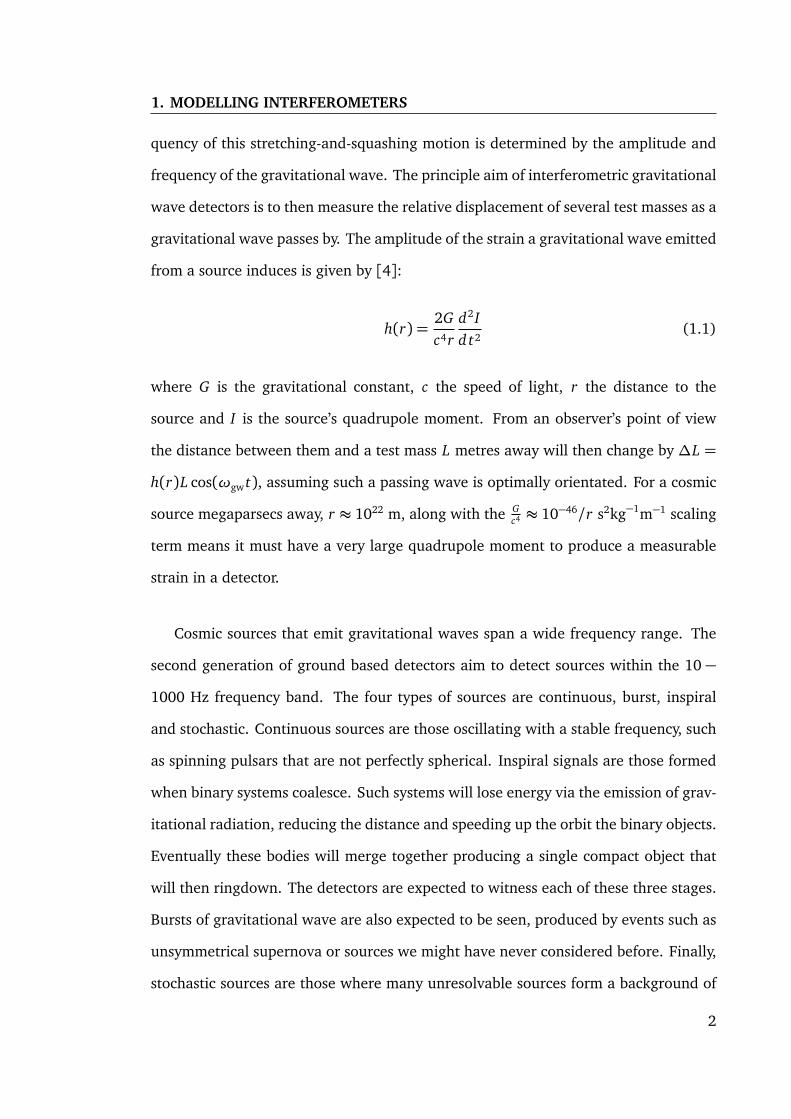
quency of this stretching-and-squashing motion is determined by the amplitude and
frequency of the gravitational wave. The principle aim of interferometric gravitational
wave detectors is to then measure the relative displacement of several test masses as a
gravitational wave passes by. The amplitude of the strain a gravitational wave emitted
from a source induces is given by [4]:
h(r) =2Gc4r
d2Id t2
(1.1)
where G is the gravitational constant, c the speed of light, r the distance to the
source and I is the source’s quadrupole moment. From an observer’s point of view
the distance between them and a test mass L metres away will then change by ∆L =
h(r)L cos(ωgw t), assuming such a passing wave is optimally orientated. For a cosmic
source megaparsecs away, r ≈ 1022 m, along with the Gc4 ≈ 10−46/r s2kg−1m−1 scaling
term means it must have a very large quadrupole moment to produce a measurable
strain in a detector.
Cosmic sources that emit gravitational waves span a wide frequency range. The
second generation of ground based detectors aim to detect sources within the 10 −1000 Hz frequency band. The four types of sources are continuous, burst, inspiral
and stochastic. Continuous sources are those oscillating with a stable frequency, such
as spinning pulsars that are not perfectly spherical. Inspiral signals are those formed
when binary systems coalesce. Such systems will lose energy via the emission of grav-
itational radiation, reducing the distance and speeding up the orbit the binary objects.
Eventually these bodies will merge together producing a single compact object that
will then ringdown. The detectors are expected to witness each of these three stages.
Bursts of gravitational wave are also expected to be seen, produced by events such as
unsymmetrical supernova or sources we might have never considered before. Finally,
stochastic sources are those where many unresolvable sources form a background of
2

Phase
0 ππ/2 3π/2
Figure 1.1: Stretch-and-squash: A passing gravitational wave will stretch and squash the spacebetween free masses. Here the effect of such a wave on a ring of free masses is shown atdifferent points in the cycle of the wave. This depicts the plus polarisation of a gravitationalwave. A cross polarisation is also possible, which induces the same stretch-and-squash effectbut rotated by 45 from the plus polarisation.
signal that can be measured. The binary coalescence rate at which events will be
seen varies greatly: for the second generation of detectors operating at designed sen-
sitivities it is expected between 0.4–400 Neutron star, 0.4–1000 blackhole and 0.2–10
neutron-blackhole binary coalescences will be seen per year [6]. Expected continuous
sources, such as the Crab and Vela pulsars, allow for targeted searches in the data that
have so far have only placed upper limits on the amount of radiation such sources
emit [7].
Thus far, the first generation of gravitational wave detectors have been constructed
and operated but have yet to detect any gravitational waves: GEO600 [8] based in
Germany, LIGO [9] in Livingston (LLO) and Hanford (LHO) and VIRGO [10] in Italy.
Advanced LIGO [11] (aLIGO) and Advanced VIRGO [12] has already begun extensive
second generation upgrades with the aim to provide a ten-fold improvement in sensi-
tivity. A new detector in Japan called KAGRA [13] is currently under construction with
another LIGO detector having been proposed for construction in India. At the heart
of all the above is a Michelson interferometer which measures the differential change
in length of space over several kilometres. Such long distances are used to maximise
the change in length as ∆L∝ L.
3

1. MODELLING INTERFEROMETERS
The LIGO detectors aim to measure the distance between two test masses placed
4 km apart. The typical strains expected from cosmic sources that it aims to detect
are very small [4]. For example, the signal from the coalescence of a binary neutron
star system ≈ 100 Mpc away is expected to have a strain amplitude of h≈ 10−22. The
resulting change in distance between these two test masses from such a source would
then be of the order ∆L = h · 4km ≈ 4 · 10−19m: a truly minute quantity. As will be
discussed in the following sections, such small changes in length are easily masked by
a variety of noise sources.
The span of expertise required to construct a detector with such unprecedented
sensitivity requires a worldwide effort. The LIGO scientific collaboration aims to do
just that. It brings together groups with knowledge from small quantum fluctuations
of light to the cosmic reach of colliding black holes to develop, construct and operate
these detectors with which we can view the universe through. This thesis is concerned
with just a few aspects of this wide range of topics: the advancement of optical mod-
elling software used for current and future generations of gravitational wave detectors
and improving the detector’s performance.
Interferometric simulations
The central aim for using interferometric simulations are to the study important phys-
ical features of increasingly complex systems for improving their sensitivity and oper-
ation. The first optical propagation codes begun to appear in 1988, written by Jean
Yves-Vinet [14]. This foundation was used in 1990 to study how deformations in
the optical components affected the interferometer [15]. These codes gradually ex-
panded into ever more complex simulation tools attempting to combine not only the
optics but also control system feedback and mechanical suspensions of the experi-
mental setups [16, 17]. As the interest and utility of these simulations tools began
to grow a series of workshops called Software tools for advanced interferometer con-
4

(a) Unique IP download locations (b) Unique IP downloads of FINESSE versions
Figure 1.2: Global reach [24]: Since I took over development of FINESSE, we have seen asteady increase in the number of unique downloads. Using a GEOIP lookup a rough locationof each download was found. The downloads are clustered around gravitational wave researchgroups but appear on every continent, except for Antarctica, which remains a future goal.
figurations [18] were held to focus efforts and further their development. To date,
simulations have played crucial role in every step of bringing the detectors from ideas
on paper to fully functioning systems, and as their complexity grows these tools will
only ever become more important.
Several branches of simulation tools exist in the gravitational wave community
today. Firstly, the full system simulations (typically time-domain models) enable optic,
suspension and electronic components to be combined and studied. Two such tools
were developed at LIGO and VIRGO, End-2-End [16] and SIESTA [17]. These are
heavy weight simulations. They require significant understanding of the software and
can be both complex in practice and computationally costly to run. The second branch
consists of steady state optical simulations. These are in general simpler to manipulate
and understand as a user; this is because many non-linear and transient behaviours
which the user might not be interested in are assumed away. Despite the simplification
they are still incredibly powerful tools and the most widely used. Those that are in
use today are OPTICKLE [19], MIST [20], SIS [21], OSCAR [22] and FINESSE [23]; a
webpage is available (gwic.ligo.org/simulations) that keeps track of the more
popular tools.
The simulation tool that will feature heavily throughout this thesis is FINESSE: the
5

1. MODELLING INTERFEROMETERS
Frequency domain INtErferometer Simulation SoftwarE. I took over the development
and responsibility of FINESSE around the beginning of 2013 from Andreas Freise, its
original creator; download statistics can be seen in figure 1.2 over this period. For
version 1.0 the source code was open sourced under the GPL v2 license. Since then
many physical, ergonomic and performance additions have been made ensuring that
FINESSE is capable of tackling current and future modelling tasks. The task of pro-
ducing a usable simulation tool in any field is not an easy one—and the level of work
required often underestimated. From the Git statistics, approximately 1000 commits
altering 270k lines of C code have been made by myself over the years. The actual
features this resulted in are outlined in more detail in appendix A.
The development and features implemented in FINESSE were driven by needs of
the community for design and commissioning tasks for LIGO, GEO and third genera-
tion detectors such as the Einstein Telescope [25]. This thesis reports on these features
and the modelling tasks I have undertaken for advanced detectors, in particular for
aLIGO. For those readers looking for more details on FINESSE and optical simulations
I recommend the FINESSE manual [26], the review article on gravitational wave in-
terferometry [27] and the optical simulation book chapter [28], all of which I am a
co-author of. For those readers who are interested in seeing FINESSE used in practice
I would suggest exploring the freely available aLIGO FINESSE Git repository [29] that
contains vast amounts of the modelling scripts and results undertaken for commis-
sioning activities.
1.1 Thesis overview
In this chapter I will provide an overview of the detector and its relevant components.
Then a more detailed description of the relevant optics involved in such interferome-
ters. These sections form the basis of required knowledge for later chapters that delve
6

into more specific problems.
In chapter 2 a new computational technique is applied to optical scattering calcu-
lations used to model precision interferometers. This is based on a near-optimal ap-
proach to solving overlap integrals which significantly improves simulation runtimes.
Here both the method and an example case are provided.
In chapter 3 a new method using purely optical means of reducing parametric insta-
bilities is proposed and analysed. Here the methods for computing radiation pressure
effects in interferometers are outlined and how such instabilities are modelled. This
is followed by both analytics and numerical experiments undertaken to investigate
it further. It is then demonstrated how the use of additional cavities can be used to
suppress parametric instabilities.
In chapter 4 I hope to provide an overview of the modelling work conducted for
the commissioning for one of the most advanced detector to date, Advanced LIGO.
Chapter 5 outlines the modelling undertaken to study the susceptibility of waveg-
uide grating mirrors to a problematic noise coupling for grating like structures. Grat-
ing structures couple any relative transverse displacement to an incident beam into
higher diffracted orders. A rigorous solver of Maxwell’s equations was used to study
this problem for Gaussian beams. These results of this show that waveguide grating
mirrors should not be affected by this coupling, thus removing one potential barrier
to their future use in precision interferometers.
1.2 Interferometric gravitational wave detectors
The first and second generation of gravitational wave detectors (GEO, LIGO, VIRGO
and KAGRA) are all based on Michelson interferometers. These aim to be sensitive to
gravitational waves over a wide frequency range from 10 Hz to several kilohertz. A
Michelson layout requires an incoming laser to be split into two parts at a beamsplitter.
7

1. MODELLING INTERFEROMETERS
The beamsplitter has four ports: the incoming port, the Y-arm port, the X-arm port
and the outgoing port. The incoming light field is split by the beamsplitter and will
propagate along the two arms of the Michelson, X-arm and Y-arm. At the end of each
arm the light is reflected back from the test mass, the returned light will then propagate
back along the arm to be interfered at the beamsplitter. Whether the interference of
the returned beams is constructive, destructive or something in between will depend
on how the light was distorted in the arms.
One basis in which these distortions can be described in are those which are com-
mon to both arms and those which are differential; these are also known as common
mode and differential mode effects or distortions. Common mode effects will alter each
beam in the same way; for example, if both of the arms are elongated the same ad-
ditional phase will be seen in each of the returned beams. Thus any common mode
effects do not alter the interference of the returned beams. Differential mode effects
are those where the effect is not the same in each arm, for example, if one arm gets
longer and the other shorter; these types of effects will alter how the beams interfere.
The amount of differential changes the light experiences in each arm will deter-
mine whether it interferes constructively, destructively or somewhere in between at
the incoming and outgoing ports. The power of the field at the outgoing port is
P = P0 cos2(∆φ +φoff), (1.2)
where P0 is the power of the input laser, ∆φ is the differential phase difference be-
tween each of the light fields recombining at the beamsplitter andφoff being a specially
chosen static phase offset, which shall be elaborated on more shortly.
The Michelson has different operating points at which it can be setup to run. An
operating point is the particular collective positioning of an interferometer’s mirrors
that allows it to behave in given manner. For gravitational wave detectors the Michel-
8

son is setup to operate close to what is called the dark fringe [27], φoff ≈ π/2. The
dark fringe is where the returned light from the arms interferes destructively at the
outgoing port and constructively at the incoming port. When operating in this state
the output port is also referred to as the dark port. The light power at the output is
now
P = P0 sin2(∆φ). (1.3)
Thus, if there is no differential phase differences between the arms all the light that
goes into the Michelson is returned back out of the incoming port, and P = 0 for the
dark port. This operating point is chosen so that all common mode noises, such as
laser frequency and amplitude noise which are significant noise sources, are reflected
back towards the laser and do not reach the output photodiode where the gravitational
wave signal is measured. Any differential signal
A passing gravitational wave will stretch-and-squash the arms of the Michelson, or
one arm becomes shorter whilst the other longer—if the polarisation of the wave is
aligned to the detector. The light will then accumulate a different phase in each arm
due to the displacement of the end mirrors relative to the beamsplitter
∆φ∝ Lh cos(ωgwτ), (1.4)
where ωgw is the frequency of the gravitational wave and τ is time, L is the length
of the arm and h the strain of the wave. This differential phase accumulated in the
arms results in these differentials fields interfering constructively at the dark port and
destructively at the bright, opposite to that of common mode fields. These fields with
a differential phase signal are then measured with a photodiode at the dark port, the
output of which then contains the strain signal from the gravitational wave.
The amount of power in light that contains the gravitational wave signal that
reaches the photodiode is very small as L h 1. To efficiently extract the signal a
9

1. MODELLING INTERFEROMETERS
technique called DC readout [30] is used (which is used in all current generation de-
tectors). Mentioned previously was that the detector is operated close to a perfect dark
fringe. In fact, φoff = π/2 + kδoff where δoff is a static (DC) differential arm length
offset chosen by us and k is the wavenumber. This DC offset allows a small amount
of carrier light to leak out to the dark port which beats with the field containing the
signal. By demodulating this beat the signal can be efficiently extracted. The signal
power using DC readout is [27]
Ps∝ δoffP0
ω20h
ωgwcsin
ωgw L
c
cos
ωgw
τ− L
c
, (1.5)
where ω0 is the angular frequency of the laser light and L is the average length of
the two arms. For signals up to a kilohertz and arm lengths of the order of several
kilometres it can be assumedωgw L
c 1, the amount of signal at the output is then
Ps ∼ δoffP0
ω20 Lh
c2cos
ωgwτ
. (1.6)
The metric used to quantify the performance of a detector is the noise-to-signal
ratio over the detector bandwidth (10− 5000Hz). This ratio states the sensitivity of
the detector to differential length changes of the arms. The sensitivity is improved by
increasing the amount of signal at the output photodiode or reducing noise sources;
design improvements for the second-generation detectors aim for both.
The noise that limits the sensitivity of detectors can be described as either funda-
mental or technical in nature. The main fundamental noises sources are:
- Seismic noise: The vibration of the ground is the limiting source of noise at very
low frequency ranges as ground motion displaces the test masses in each arm.
These displacements are not coherent between the arms due to geographical
separation, thus it appears as a differential signal. In practice the test masses
10

101 102 103
Frequency [Hz]
10−24
10−23
10−22
10−21
Stra
inse
nsit
vity 1/p
Hz
Quantum noiseCoating noiseSeismic noiseSuspension thermal noiseTotal noise
Figure 1.3: aLIGO-like Sensitivity: The main fundamental noise sources are seismic noise,coating thermal noise, suspension thermal noise and quantum noise. These create the typicalbucket like shape of the sensitivity common to all ground based interferometric gravitationalwave detectors. These curves were computed with the GWINC noise curve calculator [31].
are isolated from seismic motion using both passive systems, like multi-stage
pendulums [32], and active, such as the hydraulic external pre-isolators used in
aLIGO [33].
- Thermal noise: At low frequencies in the range of 10 to a few hundred Hz the
thermal vibrations of the atoms excite the vibrational modes of the suspension
wires [34, 35] and the internal modes of the test masses [36]. To reduce thermal
noise high quality low loss materials are used in structures whose resonance fre-
quencies are either much lower or higher than the signal bandwidth. The high
quality factor ensures much of the vibrational energy is contained within a nar-
row band around the resonance frequency reducing it in the signal bandwidth.
Coating thermal noise is also inversely proportional to the size of the incident
laser beam; as an increased beam size averages over a larger area of the mirror
surface vibrations [37].
- Quantum noise: Heisenberg’s uncertainty principle places a limit on the knowl-
11
1. MODELLING INTERFEROMETERS
edge of both the phase and amplitude of the light fields. This noise in the optical
field then translates into noise in the photocurrent of the output photodiode.
Quantum noise can be limiting across the signal bandwidth, which can broadly
be broken down into two effects: Shot noise at high frequencies and radiation
pressure noise at low. Shot noise is a frequency independent noise that (semi-
classically) is due to the finite number of photoelectrons in the output signal thus
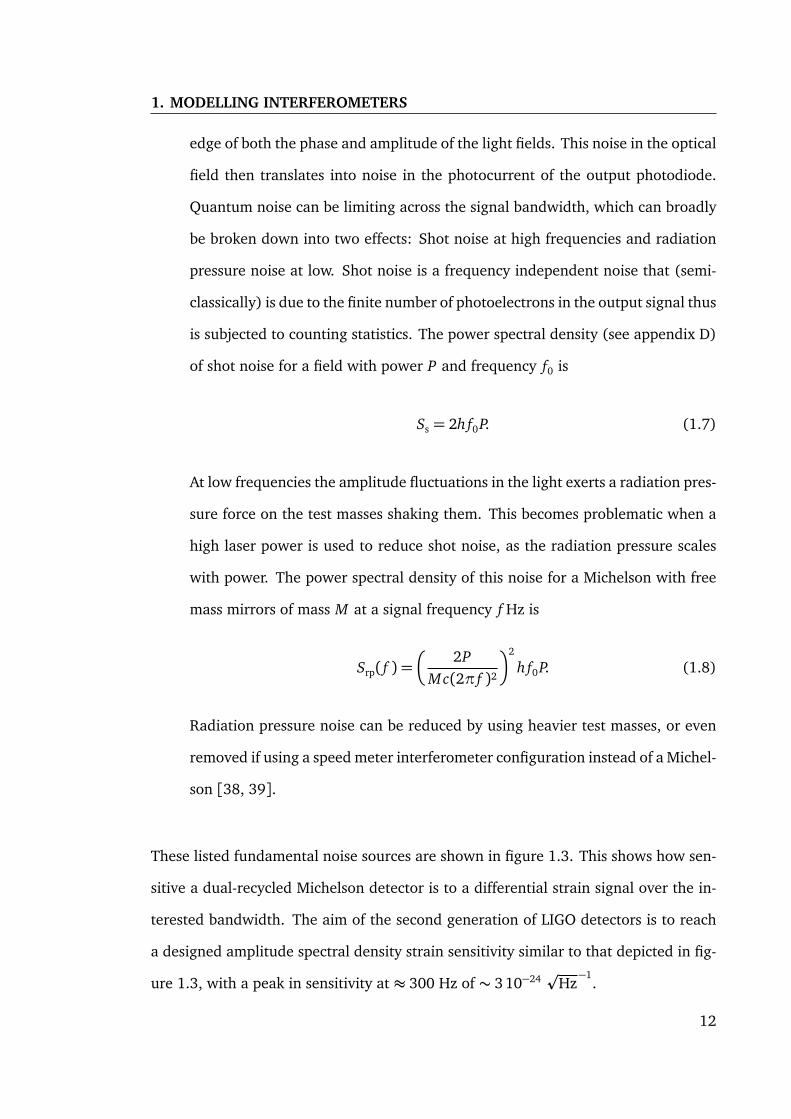
is subjected to counting statistics. The power spectral density (see appendix D)
of shot noise for a field with power P and frequency f0 is
Ss = 2hf0P. (1.7)
At low frequencies the amplitude fluctuations in the light exerts a radiation pres-
sure force on the test masses shaking them. This becomes problematic when a
high laser power is used to reduce shot noise, as the radiation pressure scales
with power. The power spectral density of this noise for a Michelson with free
mass mirrors of mass M at a signal frequency f Hz is
Srp( f ) =
2PMc(2π f )2
2
hf0P. (1.8)
Radiation pressure noise can be reduced by using heavier test masses, or even
removed if using a speed meter interferometer configuration instead of a Michel-
son [38, 39].
These listed fundamental noise sources are shown in figure 1.3. This shows how sen-
sitive a dual-recycled Michelson detector is to a differential strain signal over the in-
terested bandwidth. The aim of the second generation of LIGO detectors is to reach
a designed amplitude spectral density strain sensitivity similar to that depicted in fig-
ure 1.3, with a peak in sensitivity at ≈ 300 Hz of ∼ 3 10−24p
Hz−1
.
12
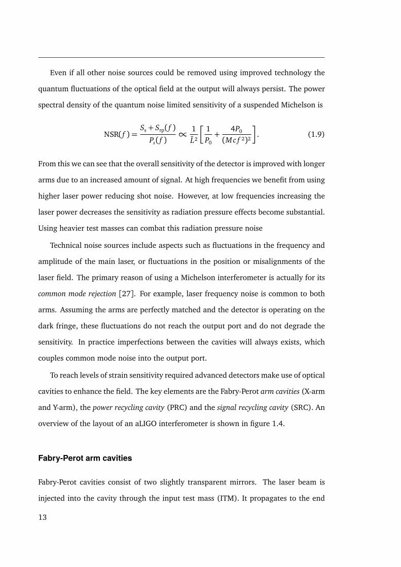
Even if all other noise sources could be removed using improved technology the
quantum fluctuations of the optical field at the output will always persist. The power
spectral density of the quantum noise limited sensitivity of a suspended Michelson is
NSR( f ) =Ss + Srp( f )
Ps( f )∝ 1
L2
1P0+
4P0
(Mc f 2)2
. (1.9)
From this we can see that the overall sensitivity of the detector is improved with longer
arms due to an increased amount of signal. At high frequencies we benefit from using
higher laser power reducing shot noise. However, at low frequencies increasing the
laser power decreases the sensitivity as radiation pressure effects become substantial.
Using heavier test masses can combat this radiation pressure noise
Technical noise sources include aspects such as fluctuations in the frequency and
amplitude of the main laser, or fluctuations in the position or misalignments of the
laser field. The primary reason of using a Michelson interferometer is actually for its
common mode rejection [27]. For example, laser frequency noise is common to both
arms. Assuming the arms are perfectly matched and the detector is operating on the
dark fringe, these fluctuations do not reach the output port and do not degrade the
sensitivity. In practice imperfections between the cavities will always exists, which
couples common mode noise into the output port.
To reach levels of strain sensitivity required advanced detectors make use of optical
cavities to enhance the field. The key elements are the Fabry-Perot arm cavities (X-arm
and Y-arm), the power recycling cavity (PRC) and the signal recycling cavity (SRC). An
overview of the layout of an aLIGO interferometer is shown in figure 1.4.
Fabry-Perot arm cavities
Fabry-Perot cavities consist of two slightly transparent mirrors. The laser beam is
injected into the cavity through the input test mass (ITM). It propagates to the end
13

1. MODELLING INTERFEROMETERS
Y-Arm
X-ArmETMXITMX
SRM
PRMIMC
OMC
BS
ITMY
ETMY
Laser
Figure 1.4: General advanced detector optical layout: On top of the base Michelson layout extracavities are included to improve the sensitivity. The notation is input test mass (ITM), end testmass (ETM), power recycling mirror (PRM), signal recycling mirror (SRM), main beamsplitter(BS), input mode cleaner (IMC) and output mode cleaner (OMC)
test mass (ETM) from which it is reflected back. If the mirrors are aligned the laser
will bounce back and forth between the mirrors. If the length of the cavity is an integer
number of the laser wavelength the optical field will resonate and the injected power
is multiplied significantly.
Increasing the length of the detector’s arms proves difficult beyond more than 4 km
due to the curvature of the Earth. By using cavities along the arms the light is made to
take multiple round trips, thus spending longer interacting with a passing gravitational
wave.
Power recycling cavity
To increase the effective power of the laser a power recycling cavity is used. This is
achieved by placing a mirror (The power recycling mirror, PRM) between the laser and
the beamsplitter. When the Michelson is operating at the dark fringe, all the common
mode light will be returned back toward the laser. Using a high reflectivity PRM the
optical field is then returned back into the Michelson. The PRC actually forms two
14

cavities, from the PRM to the ITMY and PRM to ITMX, also known as PRX and PRY
respectively. If these cavities are kept on resonance the laser power is multiplied by a
factor known as the power recycling gain, which for aLIGO is ≈ 45. By combining the
gain of the PRC and that of the arm cavities the input power is magnified greatly. The
target aLIGO input laser power is 125 W, this with the gains of the PRC and arms this
will reaches approximately 800 kW in the arm cavities.
Signal recycling cavity
Like power recycling for the common mode light, signal recycling aims to enhance any
differential signals created in the interferometer. Primarily this is aimed at enhancing
the gravitational wave signal by placing a mirror between the beamsplitter and the
output photodiode. This creates a coupled cavity between the SRC and the arms where
the gravitational wave interacts with the optical field. Two modes of operation are
available here: the signal can be resonantly enhanced at a particular frequency (signal
recycling) or the coupled cavity system can be setup so that the signal is anti-resonant
(resonant sideband extraction, RSE) which broadens the bandwidth of the detector;
the latter is used in aLIGO. An SRC operating with RSE sacrifices peak sensitivity to
allow a broader linewidth, thus the detector is less sensitive to a particular signal
frequency but better at a wider range of signals.
Mode cleaners
The spatial shape of the laser beams in these interferometers are well described by
a Gaussian beam, with perturbations to the shape described using Hermite-Gaussian
modes, which are discussed in more details in later sections. The frequency content
of the beam is also well described as a dominant single-frequency component with
sidebands describing perturbations to the beam’s phase and amplitude. The optical
field at any point in the interferometer is then described by a sum of these spatial
15

1. MODELLING INTERFEROMETERS
and frequency modes. When such an optical field is presented to a cavity only the
spatial and frequency modes that are also eigenmodes of the cavity will resonate.
Thus cavities can be designed to select particular modes of a beam and reject others:
this process is referred to as mode cleaning. Mode cleaners are just specially designed
cavities to achieve the degree of cleaning required. The two important mode cleaners
are the input mode cleaner (IMC) and output mode cleaner (OMC). The former cleans
the beam before entering the core of the interferometer and ensures a spatially and
frequency stable laser beam is used. The output mode cleaner is used to remove the
modes that do not contain any gravitational wave signal before reaching the output
photodiode. Any modes that reach it that do not contain any signal just increase the
noise and decreases the detector’s sensitivity.
Input laser
The input lasers used for gravitational wave detectors are required to be ultra-stable
and output a high power for reducing shot-noise. The pre-stabilised lasers used for
LIGO consist of a master laser whose output is amplified and stabilised before being
injected into the interferometer [40, 41]. The master laser is a commercial non-planar
ring Nd:YAG laser initially outputting 2 W, the wavelength of which is 1064 nm. This
is then boosted to ≈ 200 W in two stages using a single pass medium power amplifier
from 2 W to 35 W consisting of four Nd:YVO4 crystals and finally a high power ring
oscillator containing four further Nd:YAG crystals.
The laser output is then stabilised in frequency, power and pointing (alignment
and displacement) to achieve the required noise limits [42]. These noise sources cou-
ple to the output photodiode measuring the gravitational wave signal, thus can limit
the sensitivity. Differential imperfections in the arms—such as absorption, scattering,
and mode-mismatching—allow these noise sources to couple directly to the output
port. Using DC readout also couples these noises to the output by purposefully allow-
16

ing a small amount of carrier light through, though this level can be chosen so that
these noises are not limiting. A pre-mode cleaner is used to suppress both pointing
and power fluctuations, the output of which is directed into the IMC of the main in-
terferometer. Further, power stabilisation is achieved by monitoring fluctuations on
transmission of the IMC and fed back to an amplitude modulator before the pre-mode
cleaner. Frequency stabilisation is achieved using a monolithic reference cavity and
fed back into the master laser and a phase modulator. Overall this reaches the de-
sign requirements in the gravitational wave detection frequency band: relative power
noise of 2 · 10−8p
Hz−1
; frequency noise 0.1Hzp
Hz−1
; and relative beam pointing
noise 10−7p
Hz−1[40, 41].
1.3 Optics for gravitational wave detectors
The principal optics required for modelling gravitational wave detectors is the prop-
agation, interference and scattering of electromagnetic waves throughout the inter-
ferometer. The model must account for how these fields propagate on scales of cen-
timetres to kilometres between mirrors and through cavities, whilst including how
the beam is perturbed by imperfections in the system. A complete description of the
whole theory is not possible here. I will try to highlight the important aspects required
for this thesis, where further information on the optics relevant to gravitational wave
detectors can be found in [27].
1.3.1 Propagation of optical fields
A rigorous description of how light behaves is described by Maxwell’s equations as the
co-propagation of both an electric and magnetic field. The propagation of such light
throughout a gravitational wave detector typically involves passing through mediums
like vacuum, air, and materials such as fused silica; these materials are assumed to
17

1. MODELLING INTERFEROMETERS
be isotropic, homogeneous and non-dispersive. Continuous stable lasers are used as
the main light source this propagates between successive optical components. For
this a full Maxwellian description of the optical field is often excessive and not easily
solvable for generic interferometers. In such cases, describing light as a scalar field
and its propagation using scalar diffraction theory suffices.
Scalar diffraction describes the manner in which waves propagate and diffract from
objects in its path. As a scalar theory, it does not handle the vector nature of light. The
propagation of either the electric or magnetic field of light can be described by scalar
diffraction. For the systems that are considered in this work only the electric field, ξ,
is required to be computed; the magnetic field in such cases is always perpendicular
to the electric field with a magnitude ξ/c, where c is the speed of light.
In scalar diffraction theory the propagation of the electric field is described by the
wave equation: ∇2 − 1
v2
d2
dτ2
E(~r,τ) = 0, (1.10)
where E(~r,τ) is a complex valued scalar function describing the amplitude and phase
of the electric field:
ξ(~r,τ) = Re E(~r,τ) . (1.11)
The speed of the wave being v = c/n with n being the refractive index of the
medium it is propagating through. One potential solution to this is that of a plane-
wave propagating in the direction z, or what will be commonly referred to as the beam
axis:
E(z,τ) = E0(τ)eiωτ+i kz+iΦ(τ), (1.12)
where E0 and Φ are the amplitude and phase of the electric field, ω is the optical
angular frequency, ω = 2πc/λ and the wavenumber k = ω/c. Gravitational wave
detectors make use of several wavelengths of laser light, however the primary laser
is produced using an Nd:YAG crystal whose wavelength is λ = 1064nm; this will be
18

the default wavelength assumed throughout this thesis. Propagating the beam from
one point, z, to another, z′, along the beam axis depends only upon the time delay
between them:
E′(z′ − z,τ) = E(τ− (z′ − z)/c) = E0(τ− (z′ − z)/c)eiωτ−i k(z′−z). (1.13)
As the frequency of the optical fields in question are very high, ω/(2π)≈ 1015Hz.
Directly observing E at these frequencies is not possible; instead the measured prop-
erty is the power in the optical field which is physically achieved using either photo-
diodes or CCDs. As a photodiode cannot respond to the terahertz oscillations in the
optical field the time-averaged values of terms with the optical frequency in the power
are taken. Using the Poynting vector of E, for a plane-wave the power is:
P(τ) =ε0c2
∫
A
|E(τ)|2 dA [W] (1.14)
where the optical field has unit of V m−1. To simplify calculations the unit of E are
rescaled top
W m−1, which will be assumed from this point onwards. This then sets
the relationship between the E and the real electric field ξ as
Re E(~r,τ)=sε0c2ξ(~r,τ).
pWm−1
(1.15)
After this rescaling the power of a plane-wave optical field is
P(τ) = A|E(τ)|2, (1.16)
where A is the cross sectional area of the beam considered. When the shape of the
beam is an important feature a finite-beam size must be considered and the field in-
19

1. MODELLING INTERFEROMETERS
tensity must be integrated over the measured area:
P(τ) =
∫
A
|E(τ)|2 dA. (1.17)
1.3.2 The paraxial approximation
The aim of the paraxial approximation is to describe a beam of finite size propagating
along straight axis. Finite here means the beam is of a finite size in the transverse plane
orthogonal to the propagation axis. It is assumed the beam is like that of a plane-wave
propagating along the beam axis, z, but with a shape described by a time-independent
function u(~r). The field is then of the form
E(~r,τ) = u(~r)eiωτ−i kz. (1.18)
Substituting this into Eq.(1.10), a beam in a vacuum becomes
d2
d x2+
d2
d y2
u(~r)e−i kz +
d2
dz2[u(~r)e−i kz] + k2u(~r)e−i kz = 0. (1.19)
The z derivative here expands to
d2
dz2
u(~r)e−i kz
=
d2
dz2u(~r) + 2i k
ddz− k2u(~r)
e−i kz. (1.20)
Expanding and simplifying Eq.(1.19) further
d2
d x2+
d2
d y2+
d2
dz2
u(~r) + 2i k
ddz
u(~r) = 0. (1.21)
20

ω0
Θω(z)Rc(z)
z
zR
Figure 1.5: Gaussian beam parameters: A Gaussian beam is defined by its beam waist w0 andthe wavelength of the light. The beam diverges from this waist as it propagates along the beamaxis. This gives rise to a wavefront curvature, Rc , and far-field divergence angle Θ. The spotsize at some point along the axis is w(z). The boundary which defines the near and far field isthe Rayleigh range zR.
The paraxial approximation assumes that the beam shape does not vary quickly in
shape in the transverse plane as it propagates along the beam axis:
2kdu(~r)
dz d2u(~r)
dz2. (1.22)
Using this approximation the paraxial wave equation is given as
d2
d x2+
d2
d y2+ 2i k
ddz
u(~r) = 0. (1.23)
In practice, the paraxial approximation breaks down when describing the optical field
that diverge very quickly away from the beam axis, or similarly when trying to describe
the field at large angles from a source. Thus the paraxial approximation is not suited
for describing beams with a small source area at large distances. For describing larger
beams with small divergences that are present in gravitational wave interferometers
this approximation is a valid as it introduces minimal errors. In an aLIGO like arm
cavity the error in the total power of a beam is ≈ 10−3 ppm [43] using this description
compared to more rigorous approaches, whereas typical design requirements set losses
from absorption or clipping of mirrors are of the order of 10–100 ppm.
21

1. MODELLING INTERFEROMETERS
Various solutions exist for u(~r) in Eq.(1.23). The most prominent for optical sys-
tems is the Gaussian beam equation, which is shown in figure 1.5 with its various
defining features. This type of beam well describes the typical shape of lasers used in
gravitational wave detectors. It defines a beam whose maximal intensity is at its cen-
ter which drops off exponentially away from the beam axis. These beams are defined
by the wavelength of the laser light and the smallest size of the beam, known as the
beam waist, w0. The shape of a Gaussian beam is parameterised by the complex beam
parameter [44]:
q = z + iπw2
0
λ, (1.24)
where λ is the wavelength of the light and z is the distance along the beam axis from
the beam’s waist.
In this work the beam will be described in Cartesian coordinates. The mathematical
form of a Gaussian beam is given by [44]:
u(x , y;q) =
√√√ 2πwx(z)w y(z)
ei (Ψx (z)+Ψy (z))/2e−i k
x22qx+ y2
2qy
, (1.25)
where wx and w y are the beam spot sizes in the x and y directions, and q = qx , qyare the beam parameters in the x and y directions.
The beam has several features that are a result of the diffraction of the beam as
it passes through its narrowest width. The beam diverges as it propagates away from
the beam waist. The spot size at some point along the axis is
w(z) = w0
√√√1+
zzR
2
. (1.26)
The point at which the area the beam covers has doubled is known as the Rayleigh
range
zR =πw2
0
λ. (1.27)
22

A Gaussian beam also has a curved wavefront. The radius of curvature of a beam is
given by:
Rc(z) = z +zR
z(1.28)
where z > zR the wavefront is essentially spherical. Below the Rayleigh range the
wavefront becomes flat at the beam waist.
The beam parameter can also be reformulated in terms of the Rayleigh range
q(z) = z + i zR. (1.29)
Its inverse also contains the radius of curvature and spot size:
1q(z)
=1
Rc(z)− i
λ
πw(z)2. (1.30)
Thus it can be seen that the individual q values offer a great deal of simplification
when stating the shape of a beam at a particular point along the axis, as all of the
descriptive parameters can be derived from it.
In equation 1.25, Ψ(z) is the Gouy phase of the beam in either the x or y directions.
This is an additional longitudinal phase shift that finite beams accumulate as they
propagate compared to a plane-wave:
Ψ(z) = arctan
zzR
. (1.31)
This additional phase plays an important role in how Gaussian beams behave in an
optical cavity as will be discussed later in this section.
23

1. MODELLING INTERFEROMETERS
1.3.2.1 Hermite-Gaussian modes
Although the interferometers are constructed and designed to a high precision im-
perfections still exist: misaligned mirrors, defects on the surface of optics, thermally
distorted mirrors, to name but a few. One of the main uses of interferometer modelling
is to study how small defects can alter the behaviour of the entire interferometer. This
is predominantly the type of work that is conducted for commissioning simulations as
shown later in chapter 4. Therefore, it is important to be able to describe how a beam
is perturbed from the fundamental Gaussian beam described previously for realistic
models.
Perturbations to the transverse spatial shape of the beam are described with the ad-
dition of higher-order Gaussian modes (HOMs), in this work the Hermite-Gaussian (HG)
modes [45] which are solutions to the paraxial wave equation will be used. These
modes are based on the complete and orthonormal Hermite polynomials. The com-
plex transverse spatial amplitude of a HG modes is given by
unm(x , y,q) = un(x , qx)um(y, qy). (1.32)
The shape of the beam in the x direction can be written in terms of qx as
un(x , q) =
2π
1/4 12nn!w0
1/2q0
q
1/2
q0 q∗
q∗0 q
n/2
Hn
p2x
w(z)
exp
−i
kx2
2q
,
(1.33)
where the y direction shape is the same but given by um(y, qy). Here n defines the
order of the Hermite polynomials Hn in the x direction and m for y . The order of the
optical mode is defined as O= n+m, with individual modes referenced to as TEMnm.
TEM00, the only order zero mode, reduces to the fundamental beam. Higher order
modes typically refer to any with O > 0. The intensity of these modes is shown in
figure 1.6 for various orders. The above can also equivalently be written in terms of
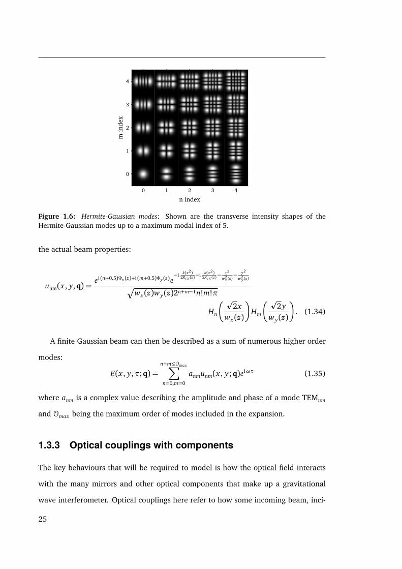
24
0 1 2 3 4
n index
0
1
2
3
4
min
dex
Figure 1.6: Hermite-Gaussian modes: Shown are the transverse intensity shapes of theHermite-Gaussian modes up to a maximum modal index of 5.
the actual beam properties:
unm(x , y,q) =ei (n+0.5)Ψx (z)+i (m+0.5)Ψy (z)e
−i k(x2)2Rcx (z)
−i k(x2)2Rcx (z)
− x2
w2x (z)− y2
w2y (z)
Æwx(z)w y(z)2n+m−1n!m!π
Hn
p2x
wx(z)
Hm
p2y
w y(z)
. (1.34)
A finite Gaussian beam can then be described as a sum of numerous higher order
modes:
E(x , y,τ;q) =n+m≤Omax∑n=0,m=0
anmunm(x , y;q)eiωτ (1.35)
where anm is a complex value describing the amplitude and phase of a mode TEMnm
and Omax being the maximum order of modes included in the expansion.
1.3.3 Optical couplings with components
The key behaviours that will be required to model is how the optical field interacts
with the many mirrors and other optical components that make up a gravitational
wave interferometer. Optical couplings here refer to how some incoming beam, inci-
25

1. MODELLING INTERFEROMETERS
dent on an imperfect component, are interfered, distorted and eventually propagate
away as the outgoing beam. Provided here is an overview of the important physical
features that are required for modelling problems tackled in later chapters of this the-
sis. More complete descriptions of these effects have been documented in the FINESSE
manual [26], the Living review article [27] and the book chapter [28].
Laser
Mirror
Reference plane
Figure 1.7: Optical fields at a mirror: Shown are the four incoming and outgoing optical fieldsat a mirror and a time dependent motion of the mirror along the beam axis.
The simplest component is a single mirror as shown in figure 1.7. Under normal
incidence, there are four beams: two incoming and two outgoing. Depending on how
reflective the mirror is for the given wavelength of light some light will be reflected,
some transmitted and some lost due to imperfections in the mirror. The mirrors used
for 1064nm light are made from fused silica with a dielectric coating stack applied to
its faces to achieve the required reflectivity. For many mirrors a high-reflectivity (HR)
coating applied to one side and an anti-reflective (AR) coating applied to the other.
Thus a mirror is defined as having three inherent properties: A power reflectivity R,
a power transmissivity T , a power loss L from absorption or scattering of the light.
These values refer to how the power of the optical field changes when interacted with,
this can also be expressed in terms of an amplitude coefficient: r =p
R and t =p
T .
The outgoing fields can be written in terms of the incoming fields:
E2(τ) = reiφr1 E1(τ) + teiφt E3(τ), (1.36)
E4(τ) = teiφt E1(τ) + reiφr2 E3(τ), (1.37)
26

where φr1 is the phase the fields picks up on reflecting from the one side, φr2 the
other, and φt on transmission. In practice the exact phase change will depend on the
details of the coating stack, such as thicknesses and materials used. However, such
information is not available to us. The important information is not the exact phase
but the relative phases between the incoming and outgoing fields. The phases must be
such that the incoming power equals that lost from scattering or absorption and the
total outgoing power, so that 1= R+ T + L. Power is conserved if in this case if [27]
φr1 +φr2 − 2φt = π(2N + 1), (1.38)
where N is any integer. The simplest choice here is that φr2 = φr2 = 0 and that
φt = π/2. This choice means reflection is a symmetric process and only transmission
receives a phase change. This phase relationship will be used throughout this thesis.
Thus the coupling equations can be written as:
E2(τ) = rE1(τ) + i tE3(τ), (1.39)
E4(τ) = i tE1(τ) + rE3(τ). (1.40)
Note that the thickness of the mirror does not play a part here. The optical fields on
both sides are in either vacuum or air; though the refractive index on either side could
also differ.
The values E1−4 all represent the amplitude and phase of the optical field relative
to a reference plane as shown in figure 1.7. The mirror can be displaced relative to this
reference plane which will alter the phase of the incoming fields. This displacement,
z as shown in the figure, is broken down into two different length scales: macroscopic
shifts for anything larger than a wavelength, and the mirror tuning, φ. The tuning is
a microscopic change in the position of the mirror, on the order of the wavelength of
27

1. MODELLING INTERFEROMETERS
the light. Typically this is stated in units of phase φ = kz, either in degrees or radians.
360 or 2π being a displacement of one wavelength. The coupling equations for a
field with identical refractive index on either side is then:
E2(τ) = rE1(τ)ei 2φ + i tE3(τ), (1.41)
E4(τ) = i tE1(τ) + rE3(τ)e−i 2φ. (1.42)
The optical fields that will be solved for in this thesis are steady state plane-wave
or paraxial fields. For either the field is described as
E1−4(τ) = a1−4eiωτ (1.43)
with a being a complex value describing the phase and amplitude of the field. In the
steady state the optical coupling equations are a set of linear equations:
a1 = b1, (1.44)
a2 = b2 + ra1ei 2φ + i ta4, (1.45)
a3 = b3, (1.46)
a4 = b4 + i ta1 + ra4e−i 2φ, (1.47)
where ~a = a1, a2, a3, a4 is the steady state amplitude of the optical field and ~b =
b1, b2, b3, b4 and the RHS of the equations are the sources of optical field at each
port. This is represented in a matrix form M ~a = ~b:
M =
1 0 0 0
−r ei 2φ 1 −i t 0
0 0 1 0
−i t 0 −r e−i 2φ 1
. (1.48)
28

Laser Input mirror End mirror
Photodiode
Beamsplitter
Sparse matrixrepresentation
Figure 1.8: Interferometer matrix: An arbitrary interferometer setup can be described usingcoupling matrices for each components as building blocks. Shown is how the interferometermatrix for a Fabry-Perot cavity and a beamsplitter would look. Here M1, M2 and B1 are theinput mirror, end mirror and beamsplitter coupling matrices. The spaces that connect thesecomponents then fill in off-diagonal elements represented by the connection matrices, C .
This is an optical coupling matrix for a mirror. For all the optical components that are
of importance for modelling gravitational wave detectors they can all be represented in
this matrix format; for a more complete list of components coupling matrices see [26].
These optical coupling matrices form the basic building blocks of an overall in-
terferometer matrix, M. This matrix describes the local coupling at each component
in the model and how each of these components are connected together. A pictorial
example of this is shown in figure 1.8. The steady state solutions of the optical fields
throughout the entire interferometer, ~a, can then be found by solving
~a =M−1~b, (1.49)
where ~b describes any source of optical fields in the interferometer, such as the main
laser.
1.3.3.1 Multiple optical frequencies
The above only describes how a single optical frequency is coupled. Gravitational
wave detectors make use of multiple optical fields at various frequencies for sensing
and controlling mirror positions [46] and for heterodyne readout of the gravitational
29

1. MODELLING INTERFEROMETERS
wave signals; though this later gave way to DC readout which offered improved sen-
sitivity [30]. Thus models of how an interferometer responds to different frequencies
of light is crucial to simulating such control and readout problems.
Two types of modulation are important for the detectors: high frequency modu-
lations of the optical fields phase or amplitude, usually in the MHz range, typically
induced by either an electro-optic, acousto-optic modulators or dithering of an optics
tuning; and lower frequency modulations of the order of kHz and less which describe
smaller perturbations to an optical field’s phase or amplitude, such as from a gravi-
tational wave signal or thermal motion of a mirror surface. The former is typically
referred to as RF modulation and the latter audio modulation, due to the typical fre-
quency ranges used.
A phase modulated plane-wave optical field is described by
E(τ) = a(ω0)eiω0τ+i m cos(Ωτ) (1.50)
where m is the modulation index describing the strength of the modulation, a(ω0) is
the complex amplitude of the ω0 frequency field and Ω the frequency of the modula-
tion. This is expanded using a Bessel function identity [47]
ei m cos(ψ) =∞∑
k=−∞i kJk(m)e
i kψ, (1.51)
where Jk is the kth Bessel function of the first kind. Thus a phase modulated field will
be
E(τ) = a(ω0)∞∑
k=−∞i kJk(m)e
i (ω0+kΩ)τ. (1.52)
There now exists multiple oscillating fields. The k = 0 field is the main carrier, that
produced by the main laser source. For fields with k 6= 0 are known as sidebands to
the main carrier whose frequency is shifted with ω0 + kΩ. This process can also be
30

applied for amplitude modulation:
E(τ) = a(ω0)(1+m cos(Ωτ))eiω0τ, (1.53)
= a(ω0)eiω0τ
h1+
m2(eiΩτ + e−iΩτ)
i. (1.54)
The maximum order of sidebands required will depend on the strength of the mod-
ulation. First order sidebands are k = ±1, second order k = ±2, etc. For RF sidebands
in aLIGO m ∼ 0.2, thus one or two suffice. For audio sidebands which represent
small perturbative modulations (m 1) only the first order sideband is required as
Jk(m 1)→ 0 for |k| > 1. Such small modulations would adequately describe how
a gravitational wave affects the optical field, for example [48]. For these small mod-
ulations the Bessel function is approximated as Jk(m)≈ (m/2)k/k!.
The more frequencies that are included the more couplings will need to be consid-
ered. For Nf frequencies the reflected field on one side of the mirror will be:
E2(τ) =N f −1∑j=0
a2(ω j)eiω jτ =
N f −1∑j=0
hra1(ω j)e
i 2φω jω0 + i ta3(ω j)
ieiω jτ. (1.55)
The coupling at each frequency is then described by the matrix
M′(ω) =
1 0 0 0
−r(ω) ei 2φ ωω0 1 −i t(ω) 0
0 0 1 0
−i t(ω) 0 −r(ω) e−i 2φ ωω0 1
. (1.56)
The mirror displacement now depends on the optical frequency, here φ usesω0 as ref-
erence frequency is scaled appropriately. There could also be a frequency dependent
r and t, however the range of modulation frequencies is much smaller than ω0 over
which the physical properties of the mirror should not vary. Thus the frequency de-
31

1. MODELLING INTERFEROMETERS
pendence here is typically ignored. The full mirror coupling matrix for all the optical
fields is then constructed with Eq.(1.56) along the diagonals:
M⇒
M′(ω0)
M′(ω1). . .
M′(ωN f −1)
. (1.57)
The above describes a motionless mirror, which couples only between the same fre-
quencies. A process known as mirror dithering is used to modulate the phase of re-
flected light. If the dithering frequency matches the difference between any two optical
field frequencies additional non-diagonal terms will be required in the above matrix.
Such techniques are used in generating sidebands for control and length sensing of
the aLIGO OMC [49].
1.3.3.2 Higher order modes
As with the additional optical frequencies, each higher order mode is considered as a
new optical field of which must be propagated throughout the interferometer. Each
optical frequency in every beam has its own higher order modes. These must be in-
cluded into the optical coupling matrix. The number of higher order modes that must
be considered for a given maximum order is:
Nm = (Omax + 1)(Omax + 2)/2 (1.58)
The process of adapting the original plane-wave coupling matrices can be visualised as
replacing each element in the plane-wave coupling matrix with an NM×NM sub-matrix.
32

For a mirror the plane-wave mirror matrix Eq.(1.56) this becomes:
M′(ω)⇒
I 0 0 0
−r(ω) ei 2φ ωω0 K11 I −i t(ω)K12 0
0 0 I 0
−i t(ω)K21 0 −r(ω) e−i 2φ ωω0 K22 I
. (1.59)
Here I is the identity matrix and the K higher order mode scattering matrices: K 11 the
scattering of modes that occurs on reflection on one side, K 22 the other, K 12 and K 21
describe how the modes are scattered on transmission. These matrices describe how
the mapping from the incoming to the outgoing mode content of the beam.
When a field interacts with an optical component its mode content is typically
changed due to imperfections. Here scattering is defined as the relationship between
the mode content of the outgoing beam a, with a beam shape q, and the mode content
of an incoming beam a′ described with a shape q′. Further details on how these beam
parameters are chosen can be found in section 1.3.4.1. Mathematically this is found
with a = K a′ where K is known as the scattering matrix.
Consider the spatial profile of a beam reflected from on an imperfect optic E′(x , y;q′) =
A(x , y)Ein(x , y;q′), where Ein is the incident beam and A(x , y) is complex function de-
scribing the perturbation it has undergone. For example, on reflection a beam will be
clipped by the finite size of the mirror with radius Rap:
α(x , y; Rap) =
1, ifp
x2 + y2 ≤ Rap
0, otherwise. (1.60)
It will also be reflected from the surface with some height variations z(x , y). Thus,
33

1. MODELLING INTERFEROMETERS
0.10 0.05 0.00 0.05 0.10
x [m]
0.10
0.05
0.00
0.05
0.10
y [m
]
20
16
12
8
4
0
4
8
12
16
20
Su
rface
heig
ht
[nm
]
Figure 1.9: Mirror map [50, 51]: The surface height variation around the central region ofETM08 installed in the x-arm at LHO. The test mass mirrors have a diameter of 34 cm, thoughthe central part as shown is typically that which the incident beam is perturbed by. This maphas been processed to remove any piston, curvature and astigmatism modes, leaving behindthe surface errors.
both the amplitude and phase of the beam will be affected with
A(x , y) = α(x , y)ei 2k z(x ,y). (1.61)
An example of the measured surface height variations present on an aLIGO test mass
mirror can be seen in figure 1.9 [51].
The mode content of the outgoing beam E(x , y;q) is computed by projecting E′
into the outgoing beam basis q. For any incoming HOM un′m′ the amount of outgoing
unm can be computed via an overlap integral, this complex valued term is known as a
coupling coefficient:
K nm,n′m′(qx , q′x , qy , q′y ; A) =
∫∫ ∞
−∞K(λx ; x)A(x , y)K(λy ; y) d x d y , (1.62)
34

where the integral kernels K(λx ; x) and K(λy ; y) are given by
K(λx ; x) = u∗n(x , qx)un′(x , q′x) , (1.63)
K(λy ; y) = u∗m(y, qy)um′(y, q′y) , (1.64)
and the parameter vectors are given by λx = (n, n′, qx , q′x) and λy = (m, m′, qy , q′y).
There are two general cases when computing Eq.(1.62): q 6= q′ which we refer to as
mode-mismatched and q = q′ as mode-matched.
Computing the scattering matrix K requires evaluating the integral Eq.(1.62) for
each of its elements. If couplings between modes up to and including order O are
considered then the number of elements in K is Nk(O) = (O4+6O3+13O2+12O+4)/4
and the computational cost of evaluating such a large number of integrals can be very
computationally expensive. In our experience [52, 53] a typical LIGO simulation task
involving HOMs can be performed with O = 6 − 10 while in some cases, such as
those that include strong thermal distortions or clipping, a higher maximum order is
required.
In simple cases where A(x , y) = 1 or A(x , y) represents a tilted surface, analyti-
cal results are available for both mode matched and mismatched cases [54, 55]. In
general however A(x , y) is of no particular form and the integral in Eq.(1.62) must be
evaluated numerically.
It is possible to split multiple distortions into separate scattering matrices for exam-
ple if the distortion can be represented as A(x , y)B(x , y) and the coupling coefficients
become a product of two separate matrices by inserting a complete basis with the
parameter q:
K nm,n′m′(q,q′; AB) =∞∑
n,m=0
K nm,nm(q, q; A)K nm,n′m′(q,q′; B). (1.65)
35

1. MODELLING INTERFEROMETERS
Thus our scattering matrix is just the product of the two separate effects
K(q,q′; AB) = K(q, q; A)K(q,q′; B). (1.66)
By choosing q= q or q′ we can set the mode-mismatching to be in either one matrix or
the other. This is ideal as a mode-matched K is a Hermitian matrix whose symmetry
can be exploited to only compute one half of the matrix. By ensuring that this matrix
also contains any distortions that require numerical integration the computational
cost can be nearly halved. It is then possible to benefit from the fast analytic solutions
to Eq.(1.62) to account for mode-mismatching in the other matrix.
Care must be taken when separating the scattering matrices in this manner. By
separating the matrices an ordering to the distortions applied to the beam is artificially
implied. If the matrices do not commute an error will be present in the scattering
calculation. This error should be reduced by using a higher Omax , thus better satisfying
the summation in Eq.(1.65). In practice, the types of mirror distortions seen from
weakly clipped apertures and surface errors the commutation error did not appear to
alter the results significantly.
Lastly, care must be taken when the two separated distortions are solved by nu-
merical finite limited integrations. The finite limits introduce a clipping in both K ,
and when combined will include twice the amount of clipping. To solve this, the inte-
gration limits must be large enough that clipping is not an issue. Or the inverse of the
scattering matrix K(x , y;α(x , y; Rap)) can be computed. Applying this inverted scat-
tering matrix removes the clipping contribution from one of the separated K . This can
also be resolved by merging all of the applied maps into a single one and integrating
over it.
Further details regarding these scattering matrices and how to efficiently compute
them can be found in chapter 2.
36
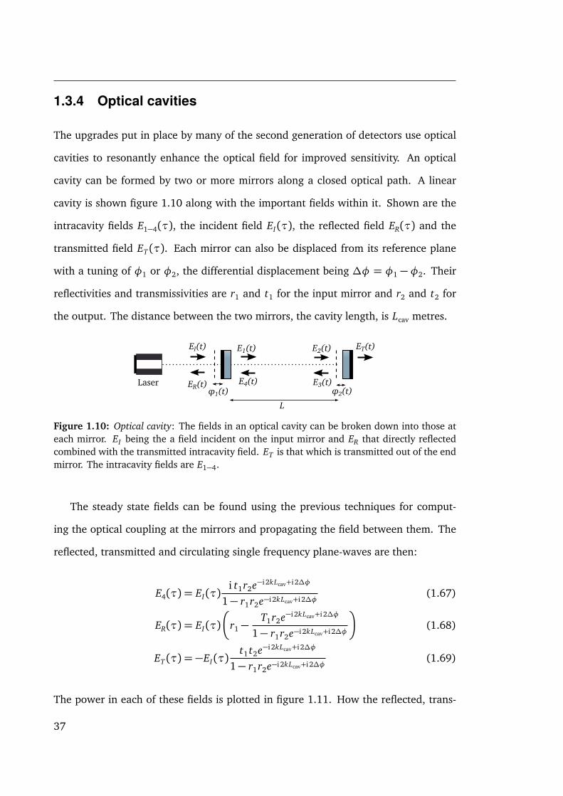
1.3.4 Optical cavities
The upgrades put in place by many of the second generation of detectors use optical
cavities to resonantly enhance the optical field for improved sensitivity. An optical
cavity can be formed by two or more mirrors along a closed optical path. A linear
cavity is shown figure 1.10 along with the important fields within it. Shown are the
intracavity fields E1−4(τ), the incident field EI(τ), the reflected field ER(τ) and the
transmitted field ET (τ). Each mirror can also be displaced from its reference plane
with a tuning of φ1 or φ2, the differential displacement being ∆φ = φ1 −φ2. Their
reflectivities and transmissivities are r1 and t1 for the input mirror and r2 and t2 for
the output. The distance between the two mirrors, the cavity length, is Lcav metres.
Laser ER(t)
EI(t) E1(t) E2(t)
E3(t)E4(t)
ET(t)
φ1(t) φ2(t)
L
Figure 1.10: Optical cavity: The fields in an optical cavity can be broken down into those ateach mirror. EI being the a field incident on the input mirror and ER that directly reflectedcombined with the transmitted intracavity field. ET is that which is transmitted out of the endmirror. The intracavity fields are E1−4.
The steady state fields can be found using the previous techniques for comput-
ing the optical coupling at the mirrors and propagating the field between them. The
reflected, transmitted and circulating single frequency plane-waves are then:
E4(τ) = EI(τ)i t1r2e−i 2kLcav+i 2∆φ
1− r1r2e−i 2kLcav+i 2∆φ(1.67)
ER(τ) = EI(τ)
r1 −
T1r2e−i 2kLcav+i 2∆φ
1− r1r2e−i 2kLcav+i 2∆φ
(1.68)
ET (τ) = −EI(τ)t1 t2e−i 2kLcav+i 2∆φ
1− r1r2e−i 2kLcav+i 2∆φ(1.69)
The power in each of these fields is plotted in figure 1.11. How the reflected, trans-
37

1. MODELLING INTERFEROMETERS
−100 −50 0 50 100
∆Φ [deg]
10−4
10−3
10−2
10−1
100
101
102N
orm
alis
edpo
wer
Over-coupled
−100 −50 0 50 100
∆Φ [deg]
10−4
10−3
10−2
10−1
100
101
102Impedance matched
Reflected Transmitted Circulating
−100 −50 0 50 100
∆Φ [deg]
10−4
10−3
10−2
10−1
100
101
102Under-coupled
Figure 1.11: Cavity resonances: The reflected, transmitted and circulating fields differ in mag-nitude on resonance depending on the cavity parameters: Over-coupled (T1 > T2), impedancematched (T1 = T2) and under-coupled (T1 < T2). The cavity power is scanned by varying thetuning of the cavity to change its length on a microscopic level.
mitted and circulating fields behave depend on the R and T of each of the cavity
mirrors: R1 and T1 being that of the input mirror and R2 and T2 being that for the end.
When the cavity mirrors have identical values the cavity is referred to as impedance
matched (T1 = T2). In this case it is possible to have all light being transmitted through
the cavity; such setups are used for the IMC and OMC as minimal reflections from these
cavities are desired. An over-coupled (T1 > T2) refers to when the end mirror is more
reflective than the input, such as the aLIGO arm cavities. Here most of the power
is reflected but significant circulating power gains are possible. The other option is
under-coupled, where the end mirror is less reflective than the input.
The intracavity field resonates when the round-trip path length is some integer
N number of wavelengths. This can also be expressed in terms of which optical fre-
quencies will resonate in the cavity. This occurs whenever the round-trip propagation
phase is 2Nπ:
2kLcavN = 2Nπ f
2Lcav
c
=
2Nπ fFSR
. (1.70)
Here the free-spectral range (FSR) is the frequency separation between successive res-
onances. This is shown in figure 1.12. In this plot it can be seen that the resonances of
38

−0.2 0.0 0.2 0.4 0.6 0.8 1.0 1.2
Frequency [FSR]
0.2
0.4
0.6
0.8
1.0
Nor
mal
ised
Pow
er
FWHM
∆ν
TEM00 TEM10 TEM20 TEM30 TEM40
Figure 1.12: Resonance features: There are several descriptive parameters regarding the shapeof the resonances. The FWHM highlighting the linewidth of the resonance. Also shown arehow HOMs up to Omax = 4 resonate in the cavity. Here the Gouy phase of the HOMs ensuresthe modes resonate at different ∆φ. Here ∆ν is the mode separation frequency betweensuccessive HOM resonances.
the TEM00 mode aligns with zero tuning. To simplify models it is useful to breakdown
lengths between optical components into two parts: a macroscopic λ length which
is always an integer number of wavelengths and the microscopic tuning. Then the
tuning ∆φ is defined so that the main carrier is resonant when ∆φ = 0.
The shape of the resonance is described by its peak value and the full width half
maximum (FWHM) as shown in figure 1.12. Another is the cavity’s finesse
F =FSR
FWHM. (1.71)
The finesse, similar to the quality factor of a resonator, is defined by how narrow the
linewidth of a resonance is compared to the free spectral range. It is also a measure of
how lossy a cavity is: a cavity that has a high finesse loses less optical field loss. When
the round-trip loss is small, ρ 1, the finesse can be approximated as
F ≈ 2πρ
. (1.72)
39

1. MODELLING INTERFEROMETERS
Loss here refers to any optical field that leaves the cavity, either from scattering, ab-
sorption, or transmitted through the mirrors. For example, the round-trip loss in a
LIGO arm cavity is mostly through transmission of the ITM, ρ ≈ Titm ≈ 0.014 which
means F ≈ 450.
1.3.4.1 Transforming beams with ABCD matrices and beam tracing
In order to compute the amplitude of the steady-state Hermite-Gaussian optical fields
the beam parameters, both qx and qy , must be defined for all fields in the model.
Without knowing the beam shape it is not possible to compute what Gouy phase is
accumulated on propagation or what shape dependent scattering occurs. This is re-
quired whether for modelling a single cavity or a full interferometer.
How a Gaussian beam is transformed when propagating or interacting with an op-
tical component is described using ABCD matrices [44]. For a known beam parameter
q1 in a medium with refractive index n1 that is transformed by a matrix with compo-
nents A, B, C and D, the new beam parameter is
q2 = n2
Aq1n1+ B
C q1n1+ D
, (1.73)
where n2 is the output medium index. ABCD matrices exist for various components
to describe how the x and y plane beam parameter is changed, these can be found in
many sources such as [26, 44, 27].
As previously discussed in section 1.3.3.2, in order to compute the optical scatter-
ing we require both the incoming and outgoing beam parameters. When doing this
it must be ensured that the correct beam parameters are used. The incoming beam
is that which is the correctly transformed incident beam. This is demonstrated in fig-
ure 1.13 for both reflection and transmission at a mirror. The transformations are
described by some ABCD matrices MR and M T respectively. There are two sides to
40
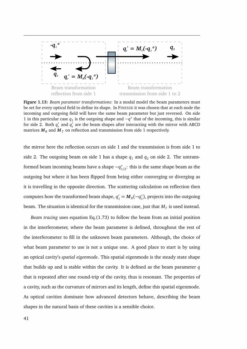
-q1*
q1
qr' = MR(-q1*)
Beam transformationreflection from side 1
q2
Beam transformationtransmission from side 1 to 2
qt' = MT(-q1*)
Figure 1.13: Beam parameter transformations: In a modal model the beam parameters mustbe set for every optical field to define its shape. In FINESSE it was chosen that at each node theincoming and outgoing field will have the same beam parameter but just reversed. On side1 in this particular case q1 is the outgoing shape and −q∗ that of the incoming, this is similarfor side 2. Both q′r and q′t are the beam shapes after interacting with the mirror with ABCDmatrices MR and M T on reflection and transmission from side 1 respectively.
the mirror here the reflection occurs on side 1 and the transmission is from side 1 to
side 2. The outgoing beam on side 1 has a shape q1 and q2 on side 2. The untrans-
formed beam incoming beams have a shape −q∗1/2: this is the same shape beam as the
outgoing but where it has been flipped from being either converging or diverging as
it is travelling in the opposite direction. The scattering calculation on reflection then
computes how the transformed beam shape, q′1 = MR(−q∗1), projects into the outgoing
beam. The situation is identical for the transmission case, just that MT is used instead.
Beam tracing uses equation Eq.(1.73) to follow the beam from an initial position
in the interferometer, where the beam parameter is defined, throughout the rest of
the interferometer to fill in the unknown beam parameters. Although, the choice of
what beam parameter to use is not a unique one. A good place to start is by using
an optical cavity’s spatial eigenmode. This spatial eigenmode is the steady state shape
that builds up and is stable within the cavity. It is defined as the beam parameter q
that is repeated after one round-trip of the cavity, thus is resonant. The properties of
a cavity, such as the curvature of mirrors and its length, define this spatial eigenmode.
As optical cavities dominate how advanced detectors behave, describing the beam
shapes in the natural basis of these cavities is a sensible choice.
41

1. MODELLING INTERFEROMETERS
The above tracing works well for a single cavity, however in the case of multiple
coupled cavities (like SRC, PRC, X-arm and Y-arm) the choice of beam parameter is
neither unique or obvious. In many cases the beam parameter traced using the eigen-
mode of one cavity will not match that of another cavity once traced to it: this is
known as a mode-mismatch. This term is used to describe whenever an optical field’s
q value does not match that of the target. If it does match, it is a mode-matched case.
More information on how to effectively trace the beam in FINESSE can be found in the
manual [26].
Mode-mismatching however is not just a numerical problem, this occurs in the
detectors and is the focus of current research as discussed in section 4.4. When a
beam is described in a mismatched basis additional higher order modes are required
to fully describe the beam, thus the beam is scattered into higher order modes. A
mismatched TEM00 beam is described with the addition of TEM20/TEM02 modes for
mismatches of a few percent, larger mismatches will require TEM40/TEM04 or higher.
The overlap between two beam parameters q1 and q2 can be compared with [56]
O(q1, q2) =4| Imq1 Imq2||q∗1 − q2|2
, (1.74)
with a value of 1 being a perfect match and 0 meaning none.
1.3.4.2 Stability
The stability of an optical cavity refers to how well it can contain a misaligned beam.
A stable cavity will ensure that the beam is kept within the geometry of the cavity. An
unstable one will eventually loose the beam after some number of round-trips. The
Hermite-Gaussian modes are only eigenmodes of stable cavities with spherical mirrors,
of which are used in gravitational wave detectors. Unstable resonators still possess a
particular spatial eigenmode [57], however, they are not analytically available in many
42

cases.
The stability of a cavity can be determined using its round-trip ABCD matrix. With
this it is possible to determine if after one round-trip the same beam shape is re-
produced, if so a stable eigenmode exists. This is achieved using equation 1.73 by
assuming q1 = q2 ≡ q (that the incoming beam is reproduced) and solving for q. If q
has a real valued beam waist, a Hermite-Gaussian mode will describe the cavity eigen-
mode [27]. If such an eigenmode exists the cavity is referred to as stable. In the case
where the solution q returns an imaginary value for the beam waist no stable eigen-
mode exists, thus the cavity is unstable. The condition for stability using the elements
of the cavity’s ABCD matrix is
0≤ A+ D+ 24
≤ 1. (1.75)
For a linear cavity this is more commonly shown as g-factors of the two mirrors:
g1 = 1− Lcav
Rc,1, (1.76)
g2 = 1− Lcav
Rc,2, (1.77)
g = g1 g2. (1.78)
which is stable for 0≤ g ≤ 1.
An important feature of a cavity’s stability is how it affects higher order modes
ability to resonate within it. As a cavity becomes more unstable the round-trip Gouy
phase approaches an integer multiple of 2π [58]:
ψRT = 2 arccos
sign(B)
√√A+ D+ 24
. (1.79)
In such cases all of the HOMs will experience the same round-trip phase, thus all are
43

1. MODELLING INTERFEROMETERS
resonant at the same time. The HOM separation frequency is
∆ν=ψRT
2πFSR. (1.80)
This states the frequency difference between successive orders of HOMs. An example
of the resonances up to order four modes being separated is shown in figure 1.12.
Whether operating a cavity in a stable or unstable state depends on its function. It
is typically desired that the mode separation frequency is higher than the linewidth of
the cavity, which allows for a single order of HOM to be resonant at once. The aLIGO
arm cavities are an example of this, where it should be ensured that the main carrier
is resonant and no other scattered modes are. The PRC and SRC are also designed to
be stable in aLIGO [59] to provide greater tolerance to scattered light, misalignments
and radius of curvature differences in mirrors. Near unstable operation also has its
uses as discussed in chapter 3 where an unstable cavity is used to manipulate multiple
HOMs.
1.3.5 Optical readout and sensing
Optical readout refers to the process of measuring information from optical fields out-
putted by the interferometer. This is primarily achieved using photodiodes to measure
a beam’s power. The photocurrent generated by a photodiode will be proportional to
the incident beam power
I(τ) = χP(τ) (1.81)
where P(τ) given by Eq.(1.16). Here χ is the efficiency of the photodiode. It will be
assumed that χ = 1 for this work being as it is a final scaling factor of an outputted
signal.
The frequency spectrum of the beam power will consist of the optical beats be-
tween the various frequency components [27]. Optical modulators will act on the
44

AS
PRC
9 MHz and 45 MHzmodulators
SRC
XARM
YARM
Signal sidebands9MHz Sidebands
Carrier field
45MHz Sidebands
REFL
POP
OMC DC
lx
ly
Lx
Ly
lp
ls
PR2
PR3
PRM
SR3
SR2
SRM
OMC
Figure 1.14: aLIGO length sensing: An overview of the aLIGO length sensing setup. Shownare the main photodiodes: REFL, POP, AS and OMC DC. Modulators are used to produce 9 and45 MHz sidebands around the carrier field. The various cavities are designed so that particularfrequencies resonant in certain areas to sense changes there. Also shown are the lengths whichdefine the interferometer DOFs as listed in table 1.1.
main carrier before it enters the core interferometer, as shown in figure 1.14. In the
case of aLIGO this is applies 9 MHz and 45 MHz phase modulation. These fields then
propagate and resonate in particular cavities to sense them. Sensing here means that
an optical field will be sensitive to changes in a particular cavity. The power in the
optical fields are then measured at various points throughout the interferometer and
phase or amplitude information is extracted by demodulating the photocurrent.
aLIGO length sensing and control design is outlined in [60]. Rather than discussing
individual mirror positions, of which there are many, several length degrees of freedom
can be defined:
- CARM: Common arm mode. This is any length changes that appears in both arm
cavities in phase, e.g. both get longer or shorter.
- DARM: Differential arm mode. This is an out of phase change in the arm lengths,
45

1. MODELLING INTERFEROMETERS
e.g. one gets longer and one gets shorter.
- MICH: This is a differential motion of the short Michelson, between the BS and
ITMs.
- SRCL: A change in the SRC length between the SRM and ITMX (SRX) and ITMY
(SRY).
- PRCL: A change in the PRC length between the PRM and ITMX (SRX) and ITMY
(SRY).
How each of these DOFs are defined in terms of actual lengths is shown in table 1.1. A
diagram of where each frequency is resonant and the important lengths for the DOFs
are shown in figure 1.14.
DOF Definition Output
PRCL (Lx − L y)/2 POP 9 MHz IMICH (Lx + L y)/2 POP 45 MHz QCARM lx − l y REFL 9 MHz ISRCL lp + (lx + l y)/2 REFL 45 MHz IDARM ls + (lx + l y)/2 OMC DC
Table 1.1: aLIGO length definitions: Each length DOF is defined in terms of the physical lengthsof the cavities as shown. These lengths are shown in figure 1.14. Also listed are the photodiodeoutputs and demodulations used for each DOF. Here REFL and POP refer to the photodiodelocations and I and Q where the in-phase or quadrature of the error signal is used.
The carrier, 9 and 45 MHz sidebands are all resonant in the PRC. In the SRC the
45 MHz sidebands resonate but the main carrier and signal sidebands are anti-resonant
to operate with resonant sideband extraction [61]. Neither of the RF sidebands res-
onate in the arm cavities. The photodiodes and demodulation frequencies used to
generate an error signal for each DOF is shown in table 1.1. All apart from DARM
are sensed using the RF sidebands. Unlike the others, DARM uses the DC power out-
putted by the diode, with some offset, on transmission of the OMC to produce its error
signal. DARM can also be sensed using the AS photodiode demodulating at 45 MHz.
The latter was used in the experiment before the OMC was commissioned.
46

−20 −15 −10 −5 0 5 10 15 20
Cavity tuning, ∆φ [deg]
−1.0
−0.5
0.0
0.5
1.0
1.5
2.0Po
wer[W]
Circulating power
Error signal [I]Error signal [Q]
Figure 1.15: Error signal example: An error signal for an optical cavity length as would beused for the Pound-Drever-Hall technique. Here the intracavity power is plotted in relation tothe error signal generated. Each resonance matches with a zero crossing in the error signal.The resonances away from∆φ = 0 are those of the RF sidebands matching the cavity. A linearrange around the zero-crossing defines the control range of the error signal.
An error signal is an output from the interferometer that can be used to stabilise
and control a particular parameter of the system. In this case, the signals outputted
by the photodiodes are demodulated with the same RF signal used to modulate the
optical fields. The error signals are used to control the cavities’ length so that they
are at the desired operating point. For optical cavities the operating point is typically
defined as one that ensures the correct optical fields are resonant or anti-resonant
within it, as noted above for each cavity.
An example of a typical shaped error signal is shown in figure 1.15. Here each of
the resonances in the cavity coincides with a zero-crossing in the error signal, either
side of which is an approximately linear change of the signal with length. This signal
would be fed into an actuator of one of the cavity mirrors controlling its longitudinal
position. A servo then keeps the error signal zeroed by displacing the mirror and
keeping the cavity on resonance, or locked. The zero crossing is crucial for this as it
provides the direction in which the actuation needs to act from the sign change. If the
mirror is displaced beyond the linear range around the zero-crossing the lock will be
lost as the servo will no longer be able to return to the resonant position.
47

1. MODELLING INTERFEROMETERS
Error signals can become distorted due to imperfections in the interferometer, such
as mode-mismatches, misalignments or scattering. This leads to either the error signal
being degraded until it is no longer usable with no zero crossing or a flat linear region.
Distortions can also lead to undesirable shifts in the operating point which is followed
by the servos. Modelling how these error signals can be designed and become distorted
is one of the strongest abilities of frequency domain simulation tools like FINESSE.
More is discussed about operating points and finding them in numerical models in
section 4.1. For interested readers, a more general overview on the aspects of length
sensing and control can be found in [27]. Whilst more specific details on the aLIGO
length and alignment can be found in [60] and [62] respectively.
1.4 Conclusion
In this chapter I have introduced what interferometric gravitational wave detectors are
and their main components in relation to their second generation upgrades. Outlined
was the core optical features that are required to construct a model that represents
these physical detectors. This introduced the core optical features that are required
to model interferometers in gravitational wave detector: propagation of lasers over
small and large distances, coupling at optical components, describing how interferom-
eter imperfections perturb the optical fields with HOMs, the handling multiple optical
frequencies for sensing and control and reading out optical signals.
The theory described here will be revisited throughout the following chapters:
chapter 2 will look at efficient computations of modal scattering; chapter 3 also re-
lies on modal scattering but here combined with radiation pressure effects to study
parametric instabilities. Chapter 4 outlines modelling work undertaken in relation
to aLIGO commissioning and design. The optical theory presented here also forms
the theoretical background of the simulation software FINESSE that I developed dur-
48

ing my PhD. An overview of FINESSE and the improvements implemented is given in
appendix A.
49

1. MODELLING INTERFEROMETERS
50

Chapter 2
Fast simulation of Gaussian-beam
mode scattering
This chapter outlines the research undertaken to speedup a major bottleneck in modal
model simulations tools using a new quadrature technique, referred to as reduced or-
der quadrature (ROQ) [63]. This work was reported in the paper Fast simulation of
Gaussian-mode scattering for precision interferometry [64] and submitted for publica-
tion. My contributions to this work were the initial idea of using reduced order meth-
ods for such problems, the development of the Python and FINESSE implementation
of the method and the numerical testing and validation of the method. The theoreti-
cal background of reduced order quadrature was contributed by Rory Smith who uses
similar techniques in data analysis of gravitational waves. Plots and text have been
used verbatim from this paper of which I was a principal author. The content has
been modified to fit into the structure of this thesis with the introductory aspects of
scattering being merged into chapter 1, hence some minor changes to the text have
been made.
Numerical integration is a key computational element for many optical simula-
51

2. REDUCED ORDER QUADRATURE
tions. Typically this is in the form of solving the propagation of light via scalar diffrac-
tion integrals, which is the approach taken in FFT based simulation tools. Modal
models take advantage of the analytic propagation of the orthogonal set of modes
that describe the spatial eigenmodes of the cavities; thus removing the scalar diffrac-
tion integral. However, when using modes to describe an imperfect optical system, the
distortions of the beam are represented by a sum of higher order optical modes. Which
modes are present depend on the incoming beam’s mode content and the imperfec-
tion. This scattering between the incoming mode and the outgoing mode content is
evaluated using multiple overlap integrals between each mode (See Eq.(1.62)).
The computational cost of this is not an issue when a small number of optical
modes are considered. Realistic models can require of order 100 modes resulting in
the number of couplings between them ranging into the 1000s. This is a significant
bottle neck in running modal simulations, like FINESSE, that include apertures, sur-
face defects, thermal distortions and other potential scattering effects. The distortions
present at a mirror usually come in a form that is colloquially referred to as a mirror
map. This is a 2D grid of data that describes how the amplitude and phase of a beam is
distorted. These maps can be based on physical measurements taken from the optics,
or could be based on some theoretical equation. The map is then integrated with both
the incoming and outgoing modes to compute the coupling between them, as shown
in Eq.(1.62). An example of an actual and crucial modelling task which required the
computation of 1000s of integrals was in the investigation of parametric instabilities.
The work described in this chapter was necessary to perform the research presented
in chapter 3.
The use of maps as seen in chapter 3 to describe distortions to a beam and how it
affects an interferometer is typical of the type of modelling performed in the gravita-
tional wave community. At hand is the task of understanding how various defects alter
the behaviour and output of the interferometer. The wide range of possible param-
52

eters of the interferometer creates a high-dimensional parameter space within which
different states must be explored. Thus, fast and lightweight numerical tools are cru-
cial for providing quick feedback to the simulator as to whether they are modelling in
a useful direction or simply to not waste time if a mistake was made.
Before ROQ, FINESSE used a basic implementation of scattering calculations. The
integration of Eq.(1.62) was done using the simplest option of a Riemann summa-
tion. Various attempts were made at improving the performance of this using multi-
threading and caching results to save recomputing similar values. The best solution
was found using the adaptive deterministic Cuhre routine provided in the Cuba li-
brary [65] along with caching as many of the computed results as possible for distor-
tions that did not vary during the simulation. These additions proved much faster than
the original Riemann summation. However, simulations could still take an excessively
long time to run (on the order of days) when simulating distortions that changed dur-
ing runtime, such as a varying thermal deformation of a mirror. At this stage Rory
Smith, working on reduced order methods for the data analysis side of gravitational
wave physics [66], and myself began exploring if such techniques could be used to
optimise problems in optics.
The ROQ can be regarded as a near-optimal, application specific, downsampling
of the integrands needed to compute the integrals for the scattering matrices. It is
analogous to a Gaussian quadrature rule, but rather than being designed to provide
exact results for polynomials of a particular degree, the ROQ produces nearly-exact
results for an arbitrary parametric function. Importantly, it is possible to place tight
error bounds on the accuracy of the ROQ for a particular application [63], thus making
it an ideal technique to speed up costly integrals whilst remaining confident in the
answer.
ROQ exploits an offline/online methodology in which the expensive integrals used
to compute scattering matrices are recast into a more computationally efficient form
53

2. REDUCED ORDER QUADRATURE
during the offline stage. The offline/online methodology involves breaking the original
computation into two parts: online refers to the computation done when the result is
needed, e.g. when a FINESSE simulation is running; offline in our case refers to a sin-
gle stage computation run separately from FINESSE which enables us to run the more
a more efficient online computation. This is then used for the rapid online evaluation
of the scattering matrices. The offline stage can itself be computationally expensive,
however this step need only be performed once and is easily parallelisable for im-
proved computation times. The data computed in the offline stage—that is needed
by the ROQ—can be stored and shared with other simulators for particular modelling
problems.
In this chapter the algorithm is shown in a general form and a working example
is used to compare against previously used integration techniques. The implementa-
tion of the method described in this article is available as open source as part of the
FINESSE source code and the Python based package PYKAT [67], which also contains
the offline computed data to enable others to model Advanced LIGO like arm cavities.
The particular implementation here is used to provide a simple, real-word example.
However, the algorithm can be easily implemented in other types of simulation tools,
for example, time domain simulations or grid based tools (also known as FFT simula-
tions) that compare beam shapes. In all cases this algorithm can significantly reduce
the computation time for evaluating overlap integrals of Gaussian modes with numer-
ical data.
The outline is as follows: section 2.1 provides the mathematical background and
algorithm for producing the ROQ (section 2.1 heavily relies on an additional math-
ematical technique known as the empirical interpolation method [68]); section 2.2
then highlights an exemplary case to demonstrate the method for modelling near-
unstable optical cavities; and finally in section 2.3 the computational performance of
the method is analysed.
54

−15 −10 −5 0 5 10 15
x [cm]
−15
−10
−5
0
5
10
15
y[c
m]
ETM07
−1.2 −0.6 0.0 0.6 1.2
Surface height [nm]
−15 −10 −5 0 5 10 15
x [cm]
−15
−10
−5
0
5
10
15
y[c
m]
ETM09
−2.2 −1.1 0.0 1.1 2.2
Surface height [nm]
−15 −10 −5 0 5 10 15
x [cm]
−15
−10
−5
0
5
10
15
y[c
m]
ITM04
−3.7 −1.9 0.0 1.9 3.7
Surface height [nm]
−15 −10 −5 0 5 10 15
x [cm]
−15
−10
−5
0
5
10
15
y[c
m]
ITM08
−1.8 −0.9 0.0 0.9 1.8
Surface height [nm]
Figure 2.1: Uncoated LIGO mirror maps [64]: Measured surface distortions for the mirrorscurrently installed in the Livingston LIGO site (shown here are the distortions of the test massesbefore they were coated). ETM09 and ITM08 are installed in the x-arm and ETM07 and ITM04in the y-arm [51]. Theses mirror maps have been processed to remove the overall mirrorcurvatures, offset and tilts.
2.1 Efficiently computing scattering matrices: inte-
gration by interpolation
For a discretely sampled mirror map with L sample points in both the x and y di-
rections, the coupling coefficient Eq.(1.62) can be approximated using a composite
Newton-Cotes quadrature rule:
knm,n′m′(qx , q′x , qy , q′y ; A)≈L∑
k=1
L∑l=1
WklK(λx ; xk)A(xk, yl)K(λy ; yl), (2.1)
where W is an L × L matrix describing the 2D composite Newton-Cotes quadrature
weights over the area of the map. Newton-Cotes rules is a term for the collection of
quadrature rules for handling equally spaced samples of the integrand. Examples of
such rules are the trapezium or Simpson’s rule. The weighting matrix is found by tak-
ing the outer product of the 1D composite Newton-Cotes quadrature weights [69] in
both x and y directions. This provides the weighting of each of the 2D samples to-
wards the integration result. There are L2 terms in the double sum Eq.(2.1). When L2
is large, L ≈ 1000 for aLIGO mirrors, there are two major bottlenecks: (i) evaluation
of the kernel at each discrete xk, yk and, (ii) evaluation of the double sum. With a set
55

2. REDUCED ORDER QUADRATURE
of M L basis elements that accurately spans the kernel space, it is possible to re-
place the double sum Eq.(2.1) with a reduced order quadrature (ROQ) rule Eq.(2.11)
containing only M2 terms, reducing the overall cost of the by a factor of ∼ L2/M2,
provided the kernel can be directly evaluated.
The reduced order quadrature scheme is implemented in three steps. The first
two are carried out offline, while the final, mirror-map-dependent step is performed
in preparation for the simulations; once per map. The steps are as follows: Step 1 -
Construct a reduced basis (offline); a set of M basis elements whose span describes
the kernel space. Step 2 - Construct an interpolant using the basis (offline) by requir-
ing it to exactly match any kernel at M carefully chosen spatial subsamples XkMk=1
[70] (and similarly for y). Step 3 - Use the interpolant to replace the inner product
evaluations in Eq.(2.1) with the ROQ Eq.(2.11) (online).
2.1.1 The empirical interpolation method
The empirical interpolation method is an efficient technique performing this offline/on-
line procedure and has been demonstrated in the context of astronomical data analysis
with LIGO [66]. Provided the kernels vary smoothly with λx over x and λy over y
then there exists a set of kernels at judiciously chosen parameter values that represent
any kernel - and hence any integral Eq.(1.62) - for an arbitrary parameter value. This
set of kernels constitutes the reduced basis: Given any parameter value λx or λy the
best approximation to the kernel at λx or λy as linear combination of the reduced
basis can be found.
The ability to exploit the reduced basis to quickly evaluate Eq.(1.62) depends on
being able to find an affine parameterisation of the integral kernels. In general, the
kernels do not admit such a parameterisation. However, the empirical interpolation
method finds a near-optimal affine approximation whose accuracy is bounded by the
accuracy of the reduced basis [63]. This affine approximation is called the empirical
56

interpolant. The spatial integrals over d x d y in Eq.(1.62) will only depend on the re-
duced basis (and hence only have to be computed once for a given mirror map) and
the parameter variation is handled by the empirical interpolant at a reduced compu-
tational cost.
The empirical interpolation method exploits the offline/online computational con-
cept where we decompose the problem into a (possibly very) expensive offline part
which allows for a computational cheap online part. In this case, the expensive offline
part is in finding the reduced basis and constructing the empirical interpolant. Once
the empirical interpolant is found then it can be used for the fast online evaluation
of Eq.(1.62). One of the main reasons why the empirical interpolant is used for fast
online evaluation of Eq.(1.62) is due to its desirable error properties that makes it su-
perior to other interpolation methods, such as polynomial interpolation. In addition,
the empirical interpolant avoids many of the pitfalls of high-dimensional interpolation
that would otherwise be encountered (see, e.g. [71]).
2.1.2 Affine parameterization
The kernel would ideally be separable for mode parameters (λx ,λy) and spatial posi-
tion (x , y). Thus a representation of the kernels would ideally have the form:
K(λx ; x) = a(λx) f (x) ,
K(λy ; y) = a(λy) f (y) . (2.2)
The functions a and f are the same irrespective of whether the kernel is a function of
x or y due to the symmetries of the Hermite Gauss modes. Using the affine parame-
terization, the coupling coefficient Eq.(1.62) is:
knm,n′m′(qx , q′x , qy , q′y) = a∗(λx)a(λy)
∫∫ ∞
−∞f ∗(x)A(x , y) f (y)d x d y , (2.3)
57
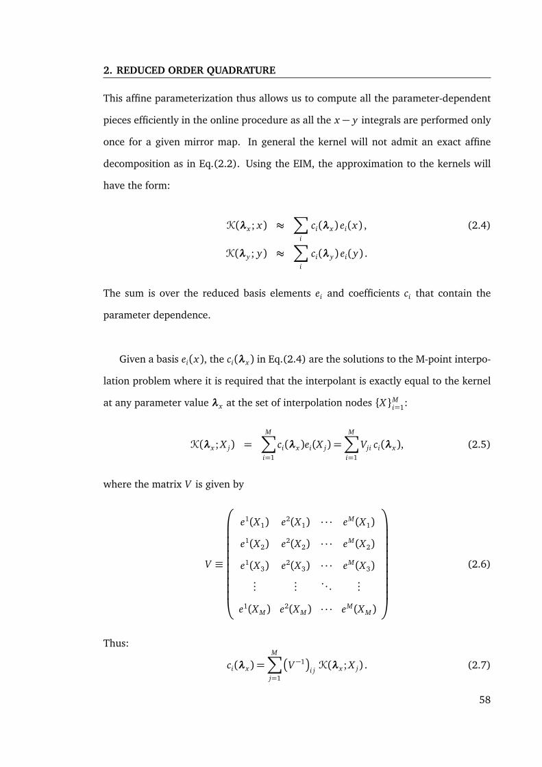
2. REDUCED ORDER QUADRATURE
This affine parameterization thus allows us to compute all the parameter-dependent
pieces efficiently in the online procedure as all the x − y integrals are performed only
once for a given mirror map. In general the kernel will not admit an exact affine
decomposition as in Eq.(2.2). Using the EIM, the approximation to the kernels will
have the form:
K(λx ; x) ≈∑
i
ci(λx) ei(x) , (2.4)
K(λy ; y) ≈∑
i
ci(λy) ei(y) .
The sum is over the reduced basis elements ei and coefficients ci that contain the
parameter dependence.
Given a basis ei(x), the ci(λx) in Eq.(2.4) are the solutions to the M-point interpo-
lation problem where it is required that the interpolant is exactly equal to the kernel
at any parameter value λx at the set of interpolation nodes X Mi=1:
K(λx ; X j) =M∑
i=1
ci(λx)ei(X j) =M∑
i=1
Vji ci(λx), (2.5)
where the matrix V is given by
V ≡
e1(X1) e2(X1) · · · eM(X1)
e1(X2) e2(X2) · · · eM(X2)
e1(X3) e2(X3) · · · eM(X3)...
.... . .
...
e1(XM) e2(XM) · · · eM(XM)
(2.6)
Thus:
ci(λx) =M∑
j=1
V−1
i jK(λx ; X j) . (2.7)
58

Substituting Eq.(2.7) into Eq.(2.4), the empirical interpolant is:
IM[K](λx ; x) =M∑
j=1
K(λx ; X j)B j(x) (2.8)
where:
B j(x)≡M∑
i=1
ei(x)V−1
i j
(2.9)
and is independent of λx . The special spatial points XkMk=1, selected from a discrete
set of points along x , as well as the basis can be found using algorithm. 1 which is
described in the next section.
Note that the kernels K(λx ; x) appear explicitly on the right hand side of Eq.(2.8).
Because of this, the kernel at the empirical interpolation nodes XkMk=1 must be di-
rectly evaluated. Fortunately this is possible in this case as a closed form of the ker-
nels is known. If the kernels were solutions to ordinary or partial differential equations
that needed to be evaluated numerically then using the empirical interpolant becomes
more challenging, however, this is not required here (see, e.g., [72, 70, 73] for ap-
plications of the empirical interpolation method to ordinary and partial differential
equation solvers).
2.1.3 The empirical interpolation method algorithm (Offline)
The empirical interpolation method algorithm solves Eq.(2.8) for arbitrary λx . While
it would be possible in principle to use arbitrary basis functions, such as Lagrange poly-
nomials which are common in interpolation problems [74, 75], a different approach
is taken that uses only the information contained in the kernels themselves. The se-
lected basis will consist of a set of M judiciously chosen kernels sampled at points on
the parameter space λixMi=1, where M is equal to the number of basis elements in
Eq.(2.8). Because the kernels vary smoothly with λx a linear combination of the basis
59
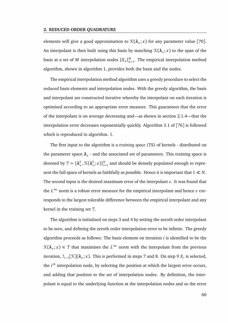
2. REDUCED ORDER QUADRATURE
elements will give a good approximation to K(λx ; x) for any parameter value [70].
An interpolant is then built using this basis by matching K(λx ; x) to the span of the
basis at a set of M interpolation nodes XkMk=1. The empirical interpolation method
algorithm, shown in algorithm 1, provides both the basis and the nodes.
The empirical interpolation method algorithm uses a greedy procedure to select the
reduced basis elements and interpolation nodes. With the greedy algorithm, the basis
and interpolant are constructed iterative whereby the interpolant on each iteration is
optimised according to an appropriate error measure. This guarantees that the error
of the interpolant is on average decreasing and—as shown in section 2.1.4—that the
interpolation error decreases exponentially quickly. Algorithm 3.1 of [76] is followed
which is reproduced in algorithm. 1.
The first input to the algorithm is a training space (TS) of kernels - distributed on
the parameter space λx - and the associated set of parameters. This training space is
denoted by T = λkx ,K(λk
x ; x)Ni=1 and should be densely populated enough to repre-
sent the full space of kernels as faithfully as possible. Hence it is important that 1 N .
The second input is the desired maximum error of the interpolant ε. It was found that
the L∞ norm is a robust error measure for the empirical interpolant and hence ε cor-
responds to the largest tolerable difference between the empirical interpolant and any
kernel in the training set T.
The algorithm is initialised on steps 3 and 4 by setting the zeroth order interpolant
to be zero, and defining the zeroth order interpolation error to be infinite. The greedy
algorithm proceeds as follows: The basis element on iteration i is identified to be the
K(λx ; x) ∈ T that maximises the L∞ norm with the interpolant from the previous
iteration, Ii−1[K](λx ; x). This is performed in steps 7 and 8. On step 9 X i is selected,
the i th interpolation node, by selecting the position at which the largest error occurs,
and adding that position to the set of interpolation nodes. By definition, the inter-
polant is equal to the underlying function at the interpolation nodes and so the error
60

Algorithm 1 Empirical Interpolation Method Algorithm: The empirical interpolation methodalgorithm builds an interpolant for the kernels Eq.(1.63) iteratively using a greedy procedure.On each iteration the current interpolant is validated against a training set T of kernels andthe worst interpolation error is identified. The interpolant is then updated so that it describesthe worst-error point perfectly. This is repeated until the worst error is less than or equal to auser specified tolerance ε.
1: Input: T = λkx ,K(λk
x ; x)Nk=1 and ε
2: Set i = 0
3: Set I0[K](λx ; x) = 0
4: Set σ0 =∞5: while σi ≥ ε do
6: i→ i + 1
7: λix = argmax
λx∈T||K(λx ; x)− Ii−1[K](λx ; x)||L∞
8: ξi(x) =K(λix ; x)
9: X i = arg maxx|ξi(x)− Ii−1[ξi](x)|
10: ei(x) =ξi(x)−Ii−1[ξi](x)ξi(X i)−Ii−1[ξi](X i)
11: Vlm = el(Xm) l ≤ i, m≤ i
12: Bm(x) =∑
l el(x)V−1
lm l ≤ i, m≤ i
13: σi =maxλx∈T||K(λx ; x)− Ii[K](λx ; x)||L∞
14: end while
15: Output: Interpolation matrix B j(x)Mj=1 and interpolation nodes X jMj=1. The equivalent
interpolant forK(λy ; y) is obtained trivially from B j(x)Mj=1 and X jMj=1 by setting x → yand X → Y .
at X i - which is the largest error on the current iteration - is removed. On step 10 the
basis function is normalised. This ensures that the matrix Eq.(2.6) is well conditioned.
On steps 11 and 12 Eq.(2.6) and Eq.(2.9) are computed, which are used to construct
the empirical interpolant Eq.(2.8). Finally, on step 13 interpolation error σi between
the interpolant on the current iteration Ii[K](λx ; x) and K(λx ; x) ∈ T as in step 7 is
calculated. The procedure is repeated until σi ≤ ε.
Once the interpolant for K(λx ; x) is found, the equivalent interpolant for K(λy ; y)
is obtained trivially from IM[K](λx ; x) by setting x → y .
61

2. REDUCED ORDER QUADRATURE
2.1.4 Error bounds on the empirical interpolant
Before proceeding to demonstrate the utility of the empirical interpolant for quickly
evaluating Eq.(1.62) a brief remark on some of the error properties of the empirical
interpolation method is made. A more detailed error analysis of the empirical in-
terpolant can be found in [63]. The empirical interpolant possess a highly desirable
property, namely exponential convergence to the desired accuracy ε. It can be shown
[76, 68] that there exists constants c > 0 and α > log(4) such that for any function f
the empirical interpolant satisfies
|| f − IM[ f ]||L∞ ≤ c e−(α−log(4))M . (2.10)
This states that under the reasonable assumption that there exists an order M in-
terpolant that allows for exponential convergence, then the empirical interpolation
method will ensure it will converge to this interpolant exponentially quickly. This is
an important property as it means that the order of the interpolant, M , tends to be
small for practical purposes. In addition, because the quantity on the right hand side
c e−(α−log(4))M is set to a user specified tolerance ε then an a priori upper bound on
the worst-fit of the interpolant can be set. However, one must still verify that the in-
terpolant describes functions outside the training a postiori, athough the error bound
should still be satisfied provided that the training set was dense enough. In fact, it can
be shown [68] that the empirical interpolation method is a near optimal solution to
the Kolmogorov n-width problem in which one seeks to find the best M -dimensional
(linear) approximation to a space of functions.
It is important to recall the integral kernels Eq.(1.63) are interpolated as a function
of six free parameters λx : two indices n and n′ and two complex beam parameters qx
and q′x . If the EIM was not used, an alternative way of expressing the λx -dependent
coefficients in Eq.(2.4) would need to be found. Consider, for example, a case in which
62

a tensor-product splines to describe the coefficients were used: Using a grid of just ten
points in each of the six parameters in λx would result in an order 106 spline which
would surely be computationally expensive to evaluate. Furthermore, there would be
no guarantee of its accuracy or convergence to a desired accuracy.
2.1.5 Reduced order quadrature (Online)
Substituting the empirical interpolant Eq.(2.8) into Eq.(2.1) gives the ROQ,
knm,n′m′(qx , q′x , qy , q′y ; A) =M∑
k=1
M∑l=1
wkl K(λx ; Xk) K(λy ; Yl) , (2.11)
with the ROQ weights ωkl given by:
ωkl =L∑
i=1
L∑j=1
Wi jA(x i, y j)Bk(x i)Bl(y j) . (2.12)
The ROQ form of the coupling coefficient enables fast online evaluations of the cou-
pling coefficients. Note that because only M2 operations are required to perform the
double sum Eq.(2.11) we expect that the ROQ is faster than the traditional L2-term
Newton-Cotes integration by a factor of L2/M2 provided that M < L. It is expected in
practice that M L due to the exponential convergence of the empirical interpolation
method.
The number of operations in Eq.(2.11) can be compressed further still due to the
separability of the empirical interpolant Eq.(2.8) into beam parameters λx and spa-
tial position x that allows us to exploit the spatial symmetry in the HG modes. The
HG modes exhibit spatial symmetry/antisymmetry under reflection about the origin.
Hence, it is useful to split the x and y dimensions into four equally sized quadrants
and perform the ROQ in each quadrant separately. For example, when a HG mode is
symmetric between two or four of the quadrants then only two or one set(s) of coef-
63

2. REDUCED ORDER QUADRATURE
0.70 0.75 0.80 0.85 0.90 0.95
Cavity stability
40
60
80
100
120
140
160
w(z)[m
m]
Beam size in cavity
ETMITM
Figure 2.2: Intracavity beam sizes [64]: The beam size on the ITM and ETM of a LIGO cavityas a function of cavity stability parameter as the mirror RoCs are tuned.
ficients K(λx ; Xk)Mk=1 needs to be computed (and likewise for K(λy ; Yl)Ml=1). This
will speed up the computation of the ROQ Eq.(2.11) by up to a factor of four. Hence,
in practice the EI is only built over one half plane for either positive or negative values
of x (or equivalently y); the basis spanning the second half-plane by reflecting the
basis about the origin is derived. To ensure that this symmetry is exploitable the data
points of the map must be distributed equally and symmetrically about the beam axis
((x , y) = (0, 0)). Those points that lie on the x and y axes must also be weighted to
take into account they contribute to multiple quadrants when the final sum is com-
puted. In the cases where the map data points are not correctly aligned a bilinear
interpolation of the data to retrieve symmetric points did not introduce any signifi-
cant errors. However, higher-order interpolation methods can introduce artefacts to
the map data.
2.2 Exemplary case: near-unstable cavities and con-
trol signals
There are several scenarios when modelling tools can benefit heavily from the ROQ
method, of particular interest are cases where the simulation time is dominated by
64

the integration time of the mirror surface maps. One such example is an investigation
into the feasibility of upgrading the LIGO interferometers with near-unstable arm cav-
ities. The stability of a Fabry-Perot cavity is determined by its length L and radius of
curvature (RoC) of each of its mirrors and can be described using the parameter::
g = (1− L/Rc,itm)(1− L/Rc,etm). (2.13)
with 0 ≤ g ≤ 1 defining the stable region. Near-unstable cavities are of interest be-
cause they result in larger beam sizes on the cavity mirrors (see also figure 2.2) which
reduces the coating thermal noise [36], one of the limiting noise sources of the detec-
tor. One negative aspect of such near-unstable cavities is that the transverse optical
mode separation frequency approaches zero as g → 0 or 1. The mode separation fre-
quency determines the difference in resonance frequency of higher-order modes with
respect to the fundamental mode. Thus, with a lower separation frequency any defect
in the cavity causing scattering into HOMs is suppressed less and can contaminate
control signals for that cavity and couple extra noise into the GW detectors output 1.
The optimal cavity design must be determined as a trade-off between these degrading
effects and the reduction in coating thermal noise. This is a typical task where a nu-
merical model can be employed to search the parameter space. In this case, each point
in that parameter space corresponds to a different beam size in the cavity which forces
a re-computation of the scattering matrices on the mirrors. Thus, the new algorithm
described here should yield a significant reduction in computing time.
In this section a summary of the test simulation results are given along with how
the model was set up. Following this an analysis of the performance of the ROQ algo-
rithm is given. ROQ integration has been implemented in FINESSE and uses the official
input parameter files for the LIGO detectors [77]. Below the preliminary investigation
1Another potential problem is additional clipping or scattering of the beam on the mirrors due tothe larger beam sizes which can result in increased round-trip losses of the arm cavity.
65

2. REDUCED ORDER QUADRATURE
of the behaviour of a single Advanced LIGO like arm cavity with a finesse of 450, where
the mirror maps for the mirrors ETM08 and ITM04 1 were applied to the high reflec-
tive (HR) surfaces is shown. This example is representative for a class of modelling
performed regularly for the LIGO commissioning and design where multiple states of
an interferometer with varying beam parameters is studied. This provides a concrete
and quantitive setup to demonstrate the required steps to use the ROQ algorithm.
−15 −10 05 0 5 10 15
Separation frequency [kHz]
0.70
0.75
0.80
0.85
0.90
0.95
Cavi
ty s
tab
l t
y, g
0
10
20
30
40
50
60
70
80
90
Ch
an
ge n
RoC
[m
]
050 0 50
ETM tun ng [deg]
10-5 10-4 10-3 10-2 10-1 100 101 102
Circulating power [W]
(a) Cavity scan as ITM and ETM RoC varied
−15 −10 −5 0 5 10 15
Separation frequency [kHz]
0.70
0.75
0.80
0.85
0.90
0.95
Cavi
ty s
tab
i it
y
−50 0 50
ETM tuning [deg]
0
10
20
30
40
50
60
70
80
90
Ch
an
ge in
RoC
[m
]
10-14 10-13 10-12 10-11 10-10
Relative error
(b) The relative error between ROQ andNewton-Cotes.
Figure 2.3: Near-unstable cavity scan with ROQ [64]: As the RoC of the ITM and ETM arevaried to make the cavity increasingly more unstable. This simulation was run for Omax = 10and includes clipping from the finite size of the mirrors and surface imperfections from theETM08 and ITM04 maps. Figure 2.3a shows how the amount of power scattering into HOMchanges as g → 1. Also visible here is the reduction in the mode separation frequency withincreasing instability. The contribution of the TEM00 mode has been removed to make theHOM content more visible. The reduced basis was built for mode order O = 14, to reduceerrors, see figure 2.8. The difference in this result when using ROQ compared to Newton-Cotes is shown in 2.3b.
Modelling the LIGO cavity for differing stabilities involves varying the RoC of both
the ITM and ETM. The resulting change in w(z) at each surface means the scattering
matrices will need to be recomputed for each chosen state. To view the HOM content
1The nominal radius of curvatures of ETM08 and ITM04 are 1934m and 2245m respectively. Theoptical properties of these mirrors were taken from [51].
66

−4 −2 0 2 4
Differential arm [deg]
−10
−5
0
5
10
Erro
rsi
gnal[W]
Evolution of Error signal
0.90
0.92
0.94
0.96
0.98
1.00
Cav
ity
stab
ility
,g
Figure 2.4: Near-unstable cavity error signal [64]: The Pound-Drever-Hall error signal for theLIGO cavity modelled in figure 2.3. A significant change in zero-crossing position and shapecan be seen as the stability of the cavity is reduced (g → 1).
0 30 60 90
Change in ETM RoC [m]
0
30
60
90
Cha
nge
inIT
MR
oC[m]
0.70
0.75
0.80
0.850.90
0.95
Stability
0 30 60 90
Change in ETM RoC [m]
0
30
60
90
Cha
nge
inIT
MR
oC[m] 0.7
0.80.9
1.0
1.1
ITM/ETM waist w0 [cm]
0 30 60 90
Change in ETM RoC [m]
0
30
60
90
Cha
nge
inIT
MR
oC[m]
2.13
2.15
2.16
2.18
2.19
ETM z [km]
0 30 60 90
Change in ETM RoC [m]
0
30
60
90
Cha
nge
inIT
MR
oC[m]
-1.8
6-1
.84
-1.8
3-1
.81
ITM z [km]
Figure 2.5: ROQ parameter space [64]: Range of beam parameters needed to model a changein curvature from 0 m to 90 m at the ITM and the ETM. In order to utilise the ROQ to coverthis parameter space, the empirical interpolant needs to be constructed using a training setmade from kernels Eq.(1.63) densely covering this space.
in the cavity created by the scattering a cavity scan can be performed, displacing one
of the cavity mirrors along the cavity axis on the order of the wavelength of the laser
light, λ = 1064 nm, to change the resonance condition of the cavity. The simulation
was performed with O = 10 with Newton-Cotes integration and the ROQ method.
The results for cavity scans at different RoCs are shown in figure 2.3a. The dominant
mode is the fundamental TEM00 whose resonance defines the zero tuning, the power
in the TEM00 mode has been removed from this plot to better show the lower power
HOM content. For more stable cavities (at the bottom of the plot in figure 2.3a) the
HOMs are well separated and not resonant at the same time as the TEM00. As the
RoC is increased, the stability is reduced and the HOMs can be seen to converge and
67

2. REDUCED ORDER QUADRATURE
eventually become resonant at a tuning of 0. At a stability of g ≈ 0.98 the cavity mode
begins to break down significantly and many modes become resonant. The effect of
this on a sensing and control signal used for a Pound-Drever-Hall control system is
shown in figure 2.4, where for increasingly unstable cavities the error signal becomes
degraded, showing an offset to the nominal zero crossing, a reduced slope and overall
asymmetry around the centre. The complete investigation into the feasibility of such
cavities was not within the original scope of this test. This would include amongst
other issues the quantitative comparison of the control noise from the degradation
of the control signals with the reduced thermal noise. The simulation task described
above is sufficient to provide a test case for the ROQ method.
2.3 Application and performance of new integration
method
In this section a complete recipe for setting up and using the ROQ for the LIGO exam-
ple, using FINESSE and PYKAT, is provided. Along with a discussion of the performance,
in terms of speed and accuracy, of the method.
2.3.1 Computing the ITM and ETM empirical interpolants
Firstly the range of beam parameters for the simulation must be determined. Once
this is known a training set can be constructed and the empirical interpolant can be
computed. The surface distortions that are of interest are those on the HR surfaces of a
LIGO arm cavity mirror. Two EIs are required: one for the ITM HR surface and one for
the ETM HR surface. This is due to the differing beam parameters at each mirror. The
beam parameter range that the training sets should span are determined by varying the
radius of curvature of the ITM and ETM to include the range of cavity stabilities that
68

are required to be modelled. The beam parameter ranges are shown in figure 2.5. The
required ranges for the ETM are 4.7 mm< w0 < 12.0 mm and 2.11 km< z < 2.20 km
and for the ITM 4.7 mm < w0 < 12.0 mm and −1.88 km < z < −1.79 km, up to
a maximum optical mode order of O = 20, Netwon-Cotes degree of 6, L = 1199.
For this example the maximum tolerable error of the empirical interpolant are set to
ε= 10−14.
Using these ranges the method described in section 2.1.1 can be used to produce
the EIs. The offline computation of the basis can have significant computational cost.
For very wide parameter ranges the memory required to store the training sets can
quickly exceed that of typical machines. For the above parameters, with 100 sample
points each in the w0 and z range, up to O= 14 and ε= 10−14 approximately 7GB of
memory was required. Running this method on machines with less memory is possible
by storing the training set on a hard drive using a suitable data storage format such as
HDF5 for access. Computation time of the empirical interpolant is then limited by the
read and write times of the media. Using a MacBook pro 2012 model which contains
a 2.7 GHz Intel core i7 with 8GB of RAM generating the ITM and ETM reduced basis
and empirical interpolant takes ≈ 4 hours each. The number of elements in the final
reduced basis for the ITM and ETM were N = 30 and N = 29 respectively.
2.3.2 Producing the ROQ weights
Once the empirical interpolant has been computed for both ITM and ETM HR surfaces
the ROQ weights Eq.(2.12) can be computed by convoluting the mirror maps with
the interpolant. The surface maps chosen are the measured surface distortions of the
(uncoated) test masses currently installed at the LIGO Livingston observatory, shown
in figure 2.1. The maps contain L ≈ 1200 samples, thus a theoretical speed-up of
L2/N 2 ≈ 12002/302 = 1600 from using ROQ over Newton-Cotes can be expected.
These maps include an aperture, A, and the variation in surface height in meters,
69

2. REDUCED ORDER QUADRATURE
−15.0 −7.5 0.0 7.5 15.0
x [cm]
−15.0
−7.5
0.0
7.5
15.0y[c
m]
ETM07 weights|w|
−15.0 −7.5 0.0 7.5 15.0
x [cm]
−15.0
−7.5
0.0
7.5
15.0
y[c
m]
log10(|arg(w)|)
−15.0 −7.5 0.0 7.5 15.0
x [cm]
−15.0
−7.5
0.0
7.5
15.0
y[c
m]
ETM09 weights|w|
−15.0 −7.5 0.0 7.5 15.0
x [cm]
−15.0
−7.5
0.0
7.5
15.0y[c
m]
log10(|arg(w)|)
−15.0 −7.5 0.0 7.5 15.0
x [cm]
−15.0
−7.5
0.0
7.5
15.0
y[c
m]
ITM04 weights|w|
−15.0 −7.5 0.0 7.5 15.0
x [cm]
−15.0
−7.5
0.0
7.5
15.0
y[c
m]
log10(|arg(w)|)
−15.0 −7.5 0.0 7.5 15.0
x [cm]
−15.0
−7.5
0.0
7.5
15.0
y[c
m]
ITM08 weights|w|
−15.0 −7.5 0.0 7.5 15.0
x [cm]
−15.0
−7.5
0.0
7.5
15.0
y[c
m]
log10(|arg(w)|)
10−5
10−4
10−3
10−2
10−1
100
Figure 2.6: Reduced order model of surface maps [64]: Absolute and argument values of theROQ weights Eq.(2.12) generated for each of the maps as shown in figure 2.1. Here the finalquadrature rule can be visualised. The top plots show the absolute value: The size of the pointis proportional to |w| and the center of each point lies on a specific empirical interpolation nodein the x-y plane (X i , Yj) (c.f. Eq.(2.5) and Eq.(2.11)). The bottom plots show log10(ar g(w)).The dashed line on each plot shows the mirror surface boundary; outside the boundary themirror maps are equal to zero. Note that there are non-zero ROQ weights associated withpoints in the region where the mirror maps are zero. While this may be counter intuitive, itis a consequence of the fact that the empirical interpolant nodes lie within the full x-y planeand, that they are constructed without any knowledge of the mirror maps: the weights stillreceive no contribution from the region where A(x , y) = 0 as this region does not contributeto the sum in Eq.(2.12). However, the ROQ uses information about the kernels Eq.(1.63) overthe entire region, including where A(x , y) = 0.
z(x , y). Thus to calculate the HOM scattering on reflection from one of these mirrors
with Eq.(1.62) the distortion term is:
A(x , y) =A(x , y)e2i kz(x ,y) (2.14)
where A(x , y) is 1 ifp
x2 + y2 < 0.16m and 0 otherwise, and k is the wavenumber
of the incident optical field.
Using Eq.(2.14) with equation Eq.(2.12) (with a Newton-Cotes rule of the same
degree the empirical interpolant was generated with) the ROQ weights can be com-
puted for each map shown in figure 2.1. This computational cost is proportional to
70

10−14 10−12 10−10 10−8 10−6
EI tolerance, ε
10−16
10−13
10−10
10−7
10−4
Rel
ativ
eer
ror
ITM08ITM04ETM07ETM09
Figure 2.7: Coupling coefficient error [64]: Relative error in the scattering matrices computedusing the ROQ and Newton-Cotes integration (with Omax = 10) as a function of the empiricalinterpolant tolerance ε. The empirical interpolant was built for maximum coupling Omax =14. The error is the minimum (dashed lines) and maximum (solid lines) over the parameterspace with which the empirical interpolant was built for, thus represents the worst and bestcase scenarios. The largest errors are independent of the map data and occur on couplingscoefficients which couple the higher order modes included in the empirical interpolant.
the number of elements in the EI, M , and the number of samples in the map, L2. For
the LIGO maps this takes ≈ 10s on a 2012 MacBook Pro. The resulting ROQ rule for
the maps can be visualised as shown in figure 2.6: the amplitude of the ROQ weights
map out the aperture and the phase of the weights varies for different maps because
of the different surface structure. The computation of these ROQ weights need only
be performed once for each map, unless the range of beam parameters required for
the empirical interpolant are changed.
To verify that the process of generating the ROQ rule has worked correctly the
scattering matrices with ROQ and Newton-Cotes across the parameter space are gen-
erated and compared. K(q; ETM07) is computed with Omax = 10 using ROQ and then
again using Newton-Cotes integration. Computing the relative error between each el-
ement of these two matrices the maximum error can be taken for q values spanning
the requested q parameter range. Figure 2.7 shows how the final error of the EI, σM ,
propagates into an error in the scattering matrix. This shows the maximum (solid line)
and minimum (dashed line) errors for any element in the scattering matrix between
the two methods. From this it can be seen that building a more accurate empirical
71

2. REDUCED ORDER QUADRATURE
4 6 8 10 12 14
Waist size [mm]
2.10
2.15
2.20
2.25
Waist position [km]
10-1410-1310-1210-1110-1010-910-810-710-610-5
Relative
error
(a) ROQ error for Omax = 10
4 6 8 10 12 14
Waist size [mm]
2.10
2.15
2.20
2.25
Waist position [km]
10-1410-1310-1210-1110-1010-910-810-710-610-5
Relative
error
(b) ROQ error for Omax = 14
4 6 8 10 12 14
Waist size [mm]
2.10
2.15
2.20
2.25
Waist position [km]
10-1410-1310-1210-1110-1010-910-810-710-610-5
Relative
error
(c) ROQ error for Omax = 18
Figure 2.8: ROQ parameter space accuracy and extrapolation [64]: Maximum relative errorbetween the scattering matrices computed for the ETM07 surface map, with ROQ and usingNewton-Cotes, for mode orders up to Omax = 18. The dashed white area represents the beam-parameter region over which training sets were generated. The subplots illustrates how usingan ROQ built for a larger Omax scattering reduces the maximum error significantly. Also shownis that the ROQ is valid over a larger parameter range than what it was initially generated for,implying that the empirical interpolant can be used for extrapolation in a limited parameterregion outside the initial range indicated by the white dashed box.
interpolant results in smaller maximum errors in the scattering matrix. Now, using
the most accurate reduced basis the maximum relative error is shown in figure 2.8
over the q space, where the white dashed box shows the boundaries of the parameters
in the training set. Overall the method successfully computed a ROQ rule that accu-
rately reproduced the Newton-Cotes results for scattering up to O = 10. It should be
noted that the largest errors, as seen in figure 2.7, do not represent the full parameter
space but occur only at smallest z and largest w0. It was also found that building a
basis including a higher maximum HOM, for example basis of order 14 for scattering
computations up to order 10, significantly improved the accuracy of the ROQ. Using a
reduced basis constructed for order 14 rather than order 10 only increased the number
of elements in the basis by 2, thus, did not significantly degrade the performance. It
can also be seen in figure 2.8 that ROQ extrapolates beyond the originally requested
q parameter space and does not instantly fail for evaluations outside of it. A gradual
decrease in the accuracy can be seen when using larger w0 values.
In figure 2.9 the convergence of the empirical interpolant error with respect to
the acceptable empirical interpolant error. One can see that the EI error converges
72

18 20 22 24 26 28 30
Basis size
10−14
10−13
10−12
10−11
10−10
10−9
10−8
10−7
10−6
EIer
ror,σ
M
ETMITM
Figure 2.9: Empirical interpolant error [64]: EI error as a function of the number of basiselements selected by the greedy algorithm (Algorithm 1) for the example described in sec-tion 2.3.1. As expected from the error analysis in section 2.1.4, the empirical interpolant errordisplays exponential convergence with the basis size.
exponentially as described in section 2.1.4.
2.3.3 Performance
The time taken to run these FINESSE simulations as O is increased is shown in fig-
ure 2.10 demonstrating how much more efficient it is to use ROQ over Newton-Cotes
for the computation of scattering matrices. Also shown for reference the computation
time when no scattering from surface maps is included to give the base time it takes
to run the rest of the FINESSE simulation. The overall speed-up achieved can be seen
in figure 2.11, reaching ≈ 2700 times faster to run the entire simulation at O = 10.
The overall speed-up then begins to drop slightly as the base time taken to run the rest
of FINESSE becomes larger. The dashed line in figure 2.11 shows the speed-up if this
base time is removed, again showing an impressive speed-up peaking at 4000 times
faster.
Using ROQ enables us to perform such modelling tasks with a far greater efficiency.
Running the model to compute the output seen in figure 2.3a required computing 100
different scattering matrices for the various changes in RoC. This took 20.5 hours
to compute with Newton-Cotes and 18 minutes with ROQ 1. The difference in the
1Note that the effective speed-up in this case is less than that in figure 2.11. Here the total runtime
73
2. REDUCED ORDER QUADRATURE
0 1 2 3 4 5 6 7 8 9 10 11 12 13 14 15
Maximum optical mode order
10−3
10−2
10−1
100
101
102
103
104
Tim
e[s]
No Maps ROQ Newton-Cotes
Figure 2.10: ROQ method timing [64]: Time taken to run FINESSE to model the steady stateoptical fields in an LIGO cavity with surface maps on both the ITM and ETM HR surfaces. Thetiming of running the entirety of FINESSE is used—rather than just the core method—becausethere are additional speed improvements from having to read and handle significantly less datapoints, from the L × L maps down to M × M ROQ weights. Smaller data fits into processorcaches better and also reduces disk read times. This plot compares a single computation ofthe scattering matrices with ROQ Eq.(2.11) and Newton-Cotes. The case with no maps usedis also shown to illustrate how much time is spent in FINESSE doing calculations not involvingmaps, which now becomes the dominant computational cost when using ROQ. A significantimprovement is also found for order zero where only one scattering integral need be calculated;this is partly time saved from having to read larger data from the disk and manipulating it inmemory. The pre-processing is unavoidable as the FINESSE can accept different types of map,thus it cannot be optimised at runtime until it know what it is dealing with. ROQ helps hereas it removes this pre-processing step so it need only happen once. The ROQ pre-processinghappens during the computing of the ROQ weights Eq.(2.12). This is a one time cost for eachmap for a particular EI and is computed outside of FINESSE, thus isn’t included in this timing.The computational cost of this is on the order of 5s for each map for the reduced basis used inthis example.
74

0 2 4 6 8 10 12 14 16
Maximum optical mode order
0
500
1000
1500
2000
2500
3000
3500
4000
4500
RO
QSp
eedu
p
Figure 2.11: ROQ speedup [64]: The speed-up achieved using ROQ compared to Netwon-Cotes as a function of mode order using the timing values in figure 2.10. The dashed line showsthe speed-up if the time for initialisation and post-processing is subtracted from both timesfor Newton-Cotes and ROQ. This demonstrates the improvements just for the computationalcost relating to map scattering calculations. Simulations that have a larger computationalcost relating to features not related to scattering will show a smaller speed-up. For example,the simulations results shown in figure 2.3 have a total simulation speed-up of ≈ 80 but thescattering calculation was reduced from ≈ 20.5 Hours→ 30s.
final result between ROQ and Newton-Cotes is shown in terms of relative error in
figure 2.3b. We have prepared the ROQ input for this example such that the error is
significantly lower than 1 ppm (relative error of 10−6) thereby showing that ROQ can
be both much faster and still sufficiently accurate.
2.4 Conclusion
Numerical modelling of optical systems plays a vital role for the design and commis-
sioning of precision interferometers. The typical use of the simulation software in
this area requires rapid iterations of many simulation runs and manual fine tuning
as modelling progresses, which is not well suited for large computer clusters. The
scope of current investigations is often limited by the required computation time and
thus the development of fast and flexible tools is a priority. Current problems in pre-
cision interferometers, such as LIGO, involve the investigation of laser beam shape
of the simulation is included. This includes the initialisation and running of the other aspects of FINESSE
which took ≈ 17 minutes. The actual time taken for just the ROQ calculation is ≈ 30 s thus a speed-upin the ROQ vs Newton-Cotes is ≈ 2500.
75

2. REDUCED ORDER QUADRATURE
distortions and their effect on the interferometer signal. Frequency-domain simula-
tions using Gaussian modes to describe the beam properties have emerged as fast and
flexible tools. However, the computation of the scattering matrix for mirror surface
distortions—effectively an overlap integral of measured surface data with Hermite-
Gauss modes—has shown to be a limiting factor in improving the computational speed
of such tools. A significant reduction in computational time of current numerical tools
is required for more efficient in-depth modelling of interferometers including more
realistic features such as clipping, optical defects, thermal distortions and parametric
instabilities.
In this work it was demonstrated how the empirical interpolation method can be
used to generate an optimised quadrature rule for paraxial optical scattering calcu-
lations, known as a reduced order quadrature. This method removes the prohibitive
computational cost of computing the scattering by speeding up the calculation of the
steady state optical fields in a LIGO arm cavity by up to a factor of 2750 times, re-
ducing simulation times from days to minutes. Using an exemplary simulation task
of near-unstable arm cavities for the LIGO interferometers it has been demonstrated
that this method is both accurate and fast for a typical modelling scenario where im-
perfections in the interferometer have a significant impact on optical performance. A
complete recipe to recreate and use the new algorithm is provided and an implemen-
tation in FINESSE. Importantly, the reduced order quadrature integration method is
generic and can be applied to any optical scattering problem for any surface distortion
data.
76
Chapter 3
Optomechanics and parametric
instabilities
This chapter outlines the research I have carried out in regards to optomechanical ef-
fects that the current and future detectors will experience. Radiation pressure effects
and parametric instabilities will limit the future sensitivity and impede the operation
of detectors. Due to my work, FINESSE has been developed and significantly extended
to allow the modelling of such optomechanical effects. Before this work no generic
interferometer simulation tool was available that combined higher order mode scat-
tering and radiation pressure effects. The development of such a tool was needed
to enable myself to study more complex systems. The result of this is a new optical
scheme that could offer a broadband reduction in parametric instabilities which is re-
ported here. This work is currently being written up for publication: Daniel Brown
et al. Optical suppression of parametric instabilities with extraction cavities. 2015. In
preparation.
In gravitational wave detectors the circulating power in the arm cavities is incred-
ibly high, ≈ 800 kW for LIGO, and the force exerted by the intracavity field on the
mirrors is non-negligible [79]. These forces can displace the cavity mirrors by multiple
77
3. OPTOMECHANICS
wavelengths of the light in some cases. This relatively large displacement, compared
to the wavelength of the light and high finesse of the cavity, is problematic in terms of
controlling a cavity. However, it is important to note that this type of large dynamic
range problem is not dealt with here, or by FINESSE. This type of problem is broadly
referred to as lock acquisition [80, 81] and can be analysed using non-linear simulation
tools such as E2E [82, 83] or SIESTA [17].
What is of interest for my work is the steady state optomechanical effects which are
the result of perturbative disturbances to the field. In such cases the interferometer is
assumed to be in a well controlled state, thus can be represented in FINESSE. Current
and future tasks for commissioning and design will undoubtedly rely on modelling that
requires such optomechanical effects to be considered. For example, on the control
scheme design of angular alignment instabilities [84, 85], or analysing parametric
instabilities; which have already been seen in low power commissioning runs at LIGO
LLO [86]. The addition of radiation pressure effects is also key for modelling on future
detector design.
Parametric instabilities (PIs) [87] are a key topic in this chapter. They are the natu-
ral vibrational modes of the mirrors, which once excited, grow exponentially in time.
This occurs when positive optomechanical feedbacks are present in the interferometer.
Eventually the amplitude of these vibrational modes become large enough that they
will cause the interferometer to lose lock.
Two effects are broadly responsible for the susceptibility of current and future gen-
erations of detectors to PIs: the increased laser power to reduce shot noise resulting in
large radiation pressure forces; and low loss materials used for test masses to reduce
thermal noise, resulting in very high quality factor materials, i.e. minimal damping of
the mechanical modes. Since 2001 such effects have been measured in various table-
top and prototype experiments [88, 89, 90] and recently during low-power commis-
sioning runs of aLIGO [86]. In the latter case a mechanical mode was ringing up to
78

+ Mechanical susceptibilityExcitation
IFO Mechanical motion to opticalOptical to mechanical force
Figure 3.1: Components of radiation pressure: An overview of the separate elements involvedin computing radiation pressure feedback that occurs in the interferometer.
the point where the LLO interferometer’s lock was lost.
As a result of previous theory and experimental evidence of PIs the need for a sim-
ulation tool that can model such effects has been apparent. Especially so for potential
commissioning issues that may arise in future high-power runs but also for designing
future detectors in such a way that may be able to mitigate such problems. An op-
tical configuration is proposed in section 3.2 that demonstrates a setup using optical
feedback to reduce the number of unstable PIs. This includes both numerical results
and analytic descriptions to describe the setup. Before this the theory of regarding the
vibrational modes and radiation pressure effects are outlined in section 3.1.1.
3.1 Radiation pressure effects
In this section, the theory involved in computing radiation pressure effects for a sus-
pended mirror including its vibrational modes and any surface distortions present is
outlined. The degrees of freedom considered are the longitudinal motion along the
surface normal and the individual vibrational modes. Rotational modes can also be
considered and have been implemented in FINESSE, the derivations for the pitch and
yaw results can be found in appendix C.
Modelling optomechanical effects will be broken down several computational steps
as shown in figure 3.1:
- Mechanical susceptibility, how the mirror’s modes respond to a particular force
79
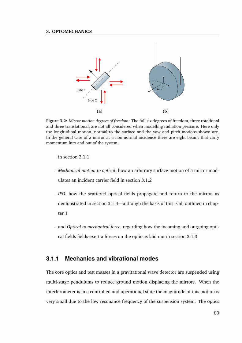
3. OPTOMECHANICS
Side 1
Side 2
(a) (b)
Figure 3.2: Mirror motion degrees of freedom: The full six degrees of freedom, three rotationaland three translational, are not all considered when modelling radiation pressure. Here onlythe longitudinal motion, normal to the surface and the yaw and pitch motions shown are.In the general case of a mirror at a non-normal incidence there are eight beams that carrymomentum into and out of the system.
in section 3.1.1
- Mechanical motion to optical, how an arbitrary surface motion of a mirror mod-
ulates an incident carrier field in section 3.1.2
- IFO, how the scattered optical fields propagate and return to the mirror, as
demonstrated in section 3.1.4—although the basis of this is all outlined in chap-
ter 1
- and Optical to mechanical force, regarding how the incoming and outgoing opti-
cal fields fields exert a forces on the optic as laid out in section 3.1.3
3.1.1 Mechanics and vibrational modes
The core optics and test masses in a gravitational wave detector are suspended using
multi-stage pendulums to reduce ground motion displacing the mirrors. When the
interferometer is in a controlled and operational state the magnitude of this motion is
very small due to the low resonance frequency of the suspension system. The optics
80

in this case are well approximated as simple harmonic oscillators. The dynamics of a
suspended mirror moving along an axis perpendicular (z) to its surface is:
Mz = −kmz − cmz +∆F(τ), (3.1)
where the dotted terms are the time derivatives and M is the mass. The restoring
force and damping of the suspension system is then described as a damped spring,
km being the spring constant and cm the damping coefficient. In Eq.(3.1) ∆F is some
externally applied force to the test mass, such as radiation pressure, in the direction
z. The transient behaviour, assuming no initial velocity or acceleration, can then be
computed by taking a Laplace transform of Eq.(3.1):
Ms2z(s) = −kmz(s)− cms z(s) +∆F(s). (3.2)
Where s = σ+ iΩ, with σ representing any exponential growth or decay and Ω being
the angular frequency of an oscillation. The resonant frequency of the suspension
is ωm =p
km/M and the damping coefficient can be reformulated in terms of the
damping ratio γm = cm/(2Mωm). The damping of the system can also be stated in
terms of the suspension quality factor, Qm = 1/(2γm).
For a given force applied to the test mass the force-to-displacement transfer func-
tion is
H(s)≡ z(s)∆F(s)
=1
M(ω2m + 2ωmγms+ s2)
. (3.3)
The steady-state case is found when σ = 0, thus s = iΩ:
H(Ω)≡ z(Ω)∆F(Ω)
=1
M(ω2m + 2iωmγmΩ−Ω2)
. (3.4)
The above is applicable for all degrees of freedom of motion and forces that are de-
scribed by simple harmonic oscillators.
81
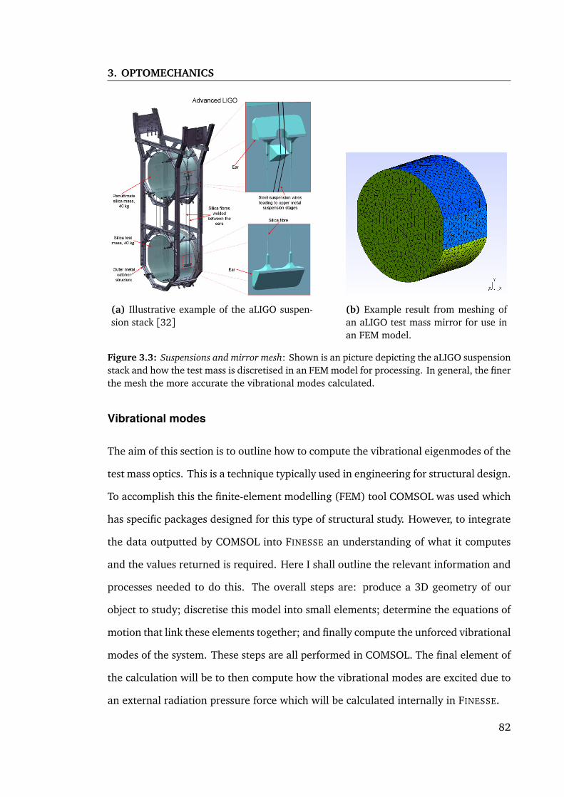
3. OPTOMECHANICS
(a) Illustrative example of the aLIGO suspen-sion stack [32]
(b) Example result from meshing ofan aLIGO test mass mirror for use inan FEM model.
Figure 3.3: Suspensions and mirror mesh: Shown is an picture depicting the aLIGO suspensionstack and how the test mass is discretised in an FEM model for processing. In general, the finerthe mesh the more accurate the vibrational modes calculated.
Vibrational modes
The aim of this section is to outline how to compute the vibrational eigenmodes of the
test mass optics. This is a technique typically used in engineering for structural design.
To accomplish this the finite-element modelling (FEM) tool COMSOL was used which
has specific packages designed for this type of structural study. However, to integrate
the data outputted by COMSOL into FINESSE an understanding of what it computes
and the values returned is required. Here I shall outline the relevant information and
processes needed to do this. The overall steps are: produce a 3D geometry of our
object to study; discretise this model into small elements; determine the equations of
motion that link these elements together; and finally compute the unforced vibrational
modes of the system. These steps are all performed in COMSOL. The final element of
the calculation will be to then compute how the vibrational modes are excited due to
an external radiation pressure force which will be calculated internally in FINESSE.
82

Parameter Value
Material Fused silicaDiameter 35 cmDepth 20 cmMass 40 kgPoisson ratio 0.17Young’s modulus 73.1 GPaDensity 2203 kg m−3
Table 3.1: Properties of the aLIGO test mass mirrors used for FEM modelling
Firstly, the geometry of the test masses needs to be constructed and the materi-
als determined for modelling in COMSOL. Using the physical dimensions of the mir-
ror [91] a computer-aided-design tool was used to construct a virtual geometry of the
mirror. The mirrors are 20 cm thick with a radius of 35 cm. The sides of the mirror
are flattened to provide a surface to bond the suspension to, an illustrative example of
which can be seen in figure 3.3a. The final geometry then undergoes a process known
as meshing, where the 3D object is broken down into a collection of tetrahedrons as
shown in figure 3.3b. Each of these tetrahedrons is known as a mass element, where
the mass of each is given by its volume times the materials density. The material used
for the aLIGO test masses is fused silica. Such a material will be considered as isotropic
and at room temperature for our modelling purposes here. The parameters used for
the material are listed in table 3.1.
How the test mass responds to both internal and external force is described by the
equations of linear elasticity. In normal operating conditions the test masses are not
subjected to any stresses that push the material beyond its yield point, thus we always
operate in a regime where Hooke’s law is applicable. The discrete elements created
during the meshing stage can then be modelled as separate masses connected to other
nearby masses via springs. The spring constant for each of these will be a function
of the Young’s Modulus and the relative displacements between the mass elements.
Such springs also need to take into account the relationship between compression
83

3. OPTOMECHANICS
and expansion as given by the Poisson ratio for the material. The calculation of these
spring constants is entirely done via COMSOL after the properties given in table 3.1
are inputted.
In general, the resulting equations of motion for each of the mass elements can be
written as:
M ~r(τ) +C ~r(τ) + K~r(τ) = ~F(τ). (3.5)
Here M , C and K are the mass, damping and stiffness matrices respectively. The
vector ~r represents the displacement of each mass element and ~F any forces applied
to them in the directions x , y and z, and ~r and ~r are the seconds and first derivative
in time. The matrices M , C and K are all symmetric where M is also diagonal. To
find the vibrational modes the unforced motion of the mass elements is first computed.
Each mode is assumed to undergo a harmonic oscillation with some amplitudesψ and
frequency ωm:
~r(τ) =ψeiωm t . (3.6)
Substituting this into Eq.(3.5), the unforced equation of motion is
−ω2mM + iωmC + K
ψeiωm t = 0. (3.7)
For non-trivial cases,ψ 6= ~0, and for any given t, the new combined matrix must equal
zero. This leaves us with solving the characteristic equation of the system to find the
eigenvalues:
detK −ω2
mM + iωmC= 0. (3.8)
Solving the Eq.(3.8) is made particularly tricky by the damping terms, C , which in
general is not a diagonal matrix. It can be assumed at this stage that the damping is
weak compared to the inertial and spring constant terms. Thus, this damping should
not not affect the eigenvalues much. Assuming a lossless system though will introduce
84

infinities when the mode is driven at its resonance. To stop this the this weak damping
can be reintroduced at a later stage by adding any small damping terms into the steady-
state equation of motion.
This is an appropriate approximation when the material being described is not
lossy. In fact, the reason PIs are problematic in the first place is partly due to pro-
ducing materials with very low internal losses, for reducing thermal noise; thus this
approximation is not an unreasonable one.
With C removed from Eq.(3.8) the characteristic equation can be solved. The
eigenvalues of this system are given by ω2m, which are the resonances squared of each
mode. The number of eigenvalues that will exist depends on the number of degrees
of freedom in our system. In this case it is 3Np for motions in x , y and z, where Np
are the number of mass elements in our mesh.
Using the mechanical mode frequencies ωm,iNp
i=1 the corresponding mechanical mode
shapes ψiNp
i=1 are found. The mode shapes are orthogonal over 3D space, ⟨ψi,ψ j⟩=Dδi j, where the factor D depends on the normalisation used. The mode shapes can be
organised into the columns of a matrix Ψ = [ψ1,ψ2, . . . ,ψNp], which is referred to as
the modal matrix. This matrix can be thought of as describing the displacement of the
mass elements in terms of the mechanical modes rather than in terms of individual
elements. Thus we can describe the motion of the optic in this modal basis:
~r(τ) = Ψ~p(τ), (3.9)
where ~p is a vector describing the amplitudes of a particular mode. The equation of
motion for each mechanical mode, using Eq.(3.5) (with no damping), is then
MΨ ~p(τ) + KΨ~p(τ) = ~F(τ). (3.10)
Using the orthogonality of the mode shapes, the mass and stiffness matrix can be
85

3. OPTOMECHANICS
diagonalised:
ΨTMΨ ~p(τ) +ΨT KΨ~p(τ) = ΨT ~F(τ), (3.11)
where ΨTMΨ ≡ M and ΨT KΨ ≡ K become the diagonalised modal mass and modal
stiffness matrices. This also defines ψTi Mψi = Mi and ψT
i Kψi = Ki which are the
modal mass and stiffness of the ith mode, which are just the diagonal elements of the
respective modal matrix. The end result of this diagonalisation is that the previously
complicated motion of the mirror becomes a set of decoupled equations of motion for
the mechanical modes. The motion for the ith mode is given by
Mi ~pi(τ) + Ki~pi(τ) = ⟨ψi, ~F(τ)⟩. (3.12)
When using FEM software, such as COMSOL, the outputs from a modal analysis of
a structure provides both the mechanical mode shapes and their resonant frequencies.
However, there is no unique combination of mode shapes and modal masses, they can
be scaled arbitrarily relative to each other [92]. There are several common scalings
used in FEM modelling, the most common of which is modal mass normalisation which
normalises the modal mass to be unitary for each mode. In this case each mode shape
is scaled by its modal mass:
ψi ≡ψiÆMi
. (3.13)
An example of modes normalised in such a way for an aLIGO like mirror can be seen
in figure 3.4. This results in a simplification of the modal masses becoming unity,
Mi ⇒ 1, and Ki ⇒ Ki/Mi =ω2m,i. The equation of motion is then
~pi(τ) +ω2m,i~pi(τ) = Fi(τ), (3.14)
with:
Fi(τ)≡ ⟨ψi, ~F(τ)⟩ (3.15)
86

defined as the modal force. This is an applied force projected onto a particular mode
shape. Finally, harmonic forces and motions, Fi(τ) = Fi(Ω)eiΩτ and ~pi(τ) = ~pi(Ω)eiΩτ,
can be considered in Eq.(3.13):
(ω2m,i −Ω2)~pi(Ω) = Fi(Ω). (3.16)
Thus for a given modal force the resulting modal motion amplitude is:
~pi(Ω) =Fi(Ω)
(ω2m,i −Ω2)
. (3.17)
Here we can see the problem with our approximation which removes the damping,
forcing at the resonant frequency results in an infinite amplitude.
Structural damping is a complex issue when the systems are particularly lossy [93].
The quality factors for the mechanical modes of the test masses are typically of the
order Qm > 106 for fused silica [94]. It is also very high for other materials being
considered for future detector upgrades such as silicon with Qm > 108 [94]. In theory
this damping should be accounted for in Eq.(3.11) with the term ΨTCΨ. It is not nec-
essarily true that Ψ will diagonalise C . With C included, Eq.(3.11) does not decouple
into a set of separate equations. Including damping would typically introduce cross
coupling between various mechanical modes. For this work, it is assumed this is a
negligible effect due to the high Qm factors. With the weak damping reintroduced,
the mechanical susceptibility for the ith mechanical mode is
Hs,i(Ω) =~pi(Ω)Fi(Ω)
=1
ω2m,i + i
ωm,i
Qm,i−Ω2
. (3.18)
The lack of any mass term here is because modal mass normalisation is used, which
gives a unitary mass values for every mechanical mode.
87

3. OPTOMECHANICS
−15.0 −7.5 0.0 7.5 15.0
x [cm]
−15.0
−7.5
0.0
7.5
15.0y[c
m]
(a) Mode 37: 15.5 kHz mechanical mode
−15.0 −7.5 0.0 7.5 15.0
x [cm]
−15.0
−7.5
0.0
7.5
15.0
y[c
m]
(b) Mode 140: 28.5 kHz mechanical mode
Figure 3.4: Example of the surface displacement for two mechanical mode shapes computedusing COMSOL for an aLIGO ETM. Both are modal mass normalised. That shown in 3.4a isthought to have been the cause of recent PIs seen at LLO [86]. The mode number is the indexof the mode generated by COMSOL.
In this section I have outlined how the mechanical vibration modes are computed
and normalised. This all happens internally within COMSOL, which outputs the mode
shapes and resonant frequencies for each mode. However, it must be ensured that the
correct modal mass normalisation is used.
3.1.2 Surface motions to optical field couplings
With the mechanical modes of the mirrors understood, the optical scattering that these
produce can be derived. The ith mechanical mode, ψi(r), describes the harmonic
3D displacement of any given point r = x , y, z within the object’s volume. As this
subsection is only concerned with the scatter from one of the mechanical modes, thus
the index i will be dropped from ψi(r) and pi for clarity. What must be extracted to
compute how the field is scattered is the displacement of the surface from which the
beam is reflected from.
The surface motion oscillating at an angular frequency Ω is calculated by selecting
88

the component along the incoming beam axis from ψ over the reflecting surface S:
zs(x , y,τ) = |p(Ω)|ψ(x , y) cos (Ωτ+∠p(Ω)) . (3.19)
The surface S is the green front facing surface as seen in figure 3.3b. The surface
motion is extracted via a dot product of the mechanical mode in the direction of the
beam axis: ψ(x , y) ≡ ψ(r)r=S · z. Here zs is a 2D surface map that can be used to
describe how the phase of the reflected beam will be perturbed by the mechanical
mode ψ(x , y). An example of such surface motion maps can be seen in figure 3.4.
Consider an optical field, EI , incident on a mirror with an amplitude reflectivity r,
some static distortion present on its surface, zo (given in meters of displacement from
a perfect surface), and a surface motion zs. The phase of the reflected field, Er , will
be perturbed by both zo and the phase modulated by zs:
Er(x , y,τ) = rEI(x , y,τ)ei 2kzs(x ,y,τ)ei 2kzo(x ,y). (3.20)
In the case where 2kzs(x , y) 1 the Bessel function expansion (See Eq.(1.51)) can
be used to describe this small perturbation with a single pair of sidebands:
Er(x , y,τ) = rEI(x , y,τ)ei 2kzo(x ,y)1+ i kzs(x , y,τ)
eiΩτ+iφs + e−iΩτ−iφs
. (3.21)
89

3. OPTOMECHANICS
The TEMnm mode of the reflected field is then given by
Er,nm(x , y,τ) = r
∫∫ ∞
∞EI(x , y,τ)ei 2kzo(x ,y)u∗nm(x , y)dx dy . . .
+ i rkp(Ω)eiΩτ + p∗(Ω)e−iΩτ
. . .
∫∫ ∞
∞EI(x , y,τ)ei 2kzo(x ,y)ψ(x , y)u∗nm(x , y)dx dy,
(3.22)
= E′r,nm + E+r,nm + E−r,nm. (3.23)
The first integral above, E′r,nm, is the direct reflection and scattering into HOMs of
any incoming carrier or signal field field. The other terms, E±r,nm, describe how the
incoming field is scattered and modulated into TEMnm of the upper and lower signal
sidebands as a result of both the surface motion and static surface distortions.
The incoming field will be a mixture of carrier fields and signal sidebands. The
incident field is described by HOMs whose amplitudes are ac, jn′m′ , at a frequency ω j:
EI(x , y,τ)≈∑
j
∑n′,m′
un′m′(x , y)ac, jn′m′eiω jτ. (3.24)
The resulting TEMnm mode of the sidebands are
E±r,nm = i rkA±s∑
j
ei (ω j±Ω)τ . . .
∑n′,m′
ac, jn′m′
∫∫ ∞
∞un′m′(x , y)ei 2kzo(x ,y)ψ(x , y)u∗nm(x , y)dx dy
. (3.25)
=∑
j
a±s, jnmei (ω j±Ω)τ (3.26)
Where A+s ≡ p(Ω) and A−s ≡ p∗(Ω), this is used to simplify the notation regarding the
90

upper sideband using the non-conjugated motion amplitude and vice-versa. Also in-
troduced here is a±s, jnm which is the upper or lower sideband amplitude for the TEMnm
mode of the jth carrier. The integral above can be separated in two separate coupling
coefficient matrices (See section 1.3.3.2): K o being the coupling due to a static dis-
tortion and K s the distortion due to the surface motion. The elements of each of the
matrices and the final amplitude of each HOM of the sideband, a±s, jnm, at a frequency
ω j ±Ω are given by:
K onmn′m′ =
∫∫ ∞
∞un′m′(x , y)ei 2kzo(x ,y)u∗nm(x , y)dx dy, (3.27)
K snmn′m′ =
∫∫ ∞
∞un′m′(x , y)ψ(x , y)u∗nm(x , y)dx dy, (3.28)
a±s, jnm = i rkA±s∑n′,m′
ac, jn′m′(Ks K o)nmn′m′ . (3.29)
The challenge now is to find computationally efficient methods for computing the
scattering matrix K s. For the lower order motions longitudinal, pitch and yaw (See ap-
pendix C for pitch and yaw) analytic solutions can be found to the integrals. However,
generic surface motions will rely on numerical integration.
In practice ψ(r) is calculated at the discrete vertices of the 3D mesh generated by
COMSOL. For this the mesh vertices along the high-reflectivity side of the mirror are
selected and the component of displacement normal to the surface is taken. The ver-
tices are not typically ordered in a grid or with a sufficient number of samples required
to accurately calculate the numerical integral when considering the scattering of high
order optical modes. A bilinear interpolator for scattered data points was found to be
suitable for generating a finer sampled grid. For many mechanical modes, or cases
where the beam parameter changes during a simulation task, it is worth considering
using reduced order quadrature (See chapter 2) for accelerating the scattering ma-
trix computation time—as was used in the PI reduction modelling at the end of this
91

3. OPTOMECHANICS
chapter.
Longitudinal motion
The simplest of the motions to consider is the longitudinal motions, or motion along
the surface normal: The shape in which the surface is displaced is then simply ψ(x , y) =
1. Thus solving Eq.(3.28) using the orthogonality of the Hermite polynomials, the re-
sulting coupling coefficients are:
K snmn′m′ = δnn′δmm′ , (3.30)
a±s, jnm = i rkZ±∑n′,m′
ac, jn′m′Konmn′m′ , (3.31)
where, (like A±s ) Z+ ≡ p(Ω) and Z− ≡ p∗(Ω) are introduced for when representing flat
longitudinal motions of a surface along the beam axis. This shows that the signal side-
bands are just phase modulations of the carrier and have a mode content determined
purely by the static surface distortions, K o.
3.1.3 Optical field to surface motion coupling
As described by Maxwell’s theory of light, a plane-wave optical field propagating in a
vacuum exerts a pressure on over a surface A proportional to its time averaged Poynt-
ing vector [79], ⟨S(τ)⟩:Frp(τ) =
∫
A
⟨S(x , y,τ)⟩c
dA. (3.32)
The field consists of N j frequencies of light ω jN j
j=1 each of which also has some weak
amplitude and phase modulation at a frequency Ω described with a pair of sidebands:
E(x , y,τ) =N j∑j=1
n+m≤Omax∑n,m
unm(x , y)(ac, jnm + a+s, jnmeiΩτ + a−s, jnme−iΩτ)eiω jτ. (3.33)
92
Firstly the radiation pressure force from plane waves will be described, following this
how higher order optical modes and mechanical modes will then be described. The
time averaged Poynting vector, also the intensity of the beam I(x , y,τ), of such a field
points in the direction of propagation and has a magnitude
I(x , y,τ)≡ ⟨S(x , y,τ)⟩= |E(x , y,τ)|2. (3.34)
The intensity will contain the beats of all frequency terms present in the beam.
Some of these beats will describe amplitude modulations of the intensity of the light,
thus a fluctuating radiation pressure force. What is of interest are the linear steady-
state oscillations. This requires making some approximations so that many of the
non-linear terms are negligible:
- That DC forces acting on mirror are balanced by control systems acting on the
mirror.
- That carrier fields and any modulated sidebands are separated by large frequen-
cies, ω j Ω. Thus any beating between two carriers or between two different
carrier’s signal sidebands will be at such a high frequency, § ω j, that the me-
chanical susceptibility, being∝ω−2j , renders such forces negligible
- There will also be frequency terms oscillating at 2Ω from the signal sidebands
beating with each other; as the magnitude of such sidebands is very small the
product between them is also negligible. Thus the only terms remaining are of
the carrier beating with its own signal sidebands.
The terms describing the fluctuation in a beam’s intensity (that we are concerned
93

3. OPTOMECHANICS
with as noted above) is
I(x , y,τ) =∑
j
∑n,m
∑n′,m′
unm(x , y)u∗n′m′(x , y)a+s, jnma∗c, jn′m′ . . .
+ u∗nm(x , y)un′m′(x , y)a−∗s, jnmac, jn′m′eiΩτ + c.c. (3.35)
Integrating over the area in which the beam is incident, the power fluctuations are
P(τ) =∑
j
∑n,m
a+s, jnma∗c, jnm + a−∗s, jnmac, jnm
eiΩτ + c.c. (3.36)
The above is just for a single beam. The momentum of both the incoming and outgoing
fields on both sides of a mirror must be accounted for. The total force on the mirror
from the incoming and outgoing beams on both sides of a mirror is
Frp(τ) =P2i(τ) + P2o(τ)− P1i(τ)− P1o(τ)
c. (3.37)
Here care must be taken with the minus sign convention for the forces. This is decided
by which direction the motion is deemed to be positive in (See figure 3.2a) 1.
A subtle point must be mentioned when it comes to computing the power fluctu-
ations with Eq.(3.36). When solving the set of linear coupling equations describing
the interferometer only linear operations can be described when using a matrix in-
version; the conjugate operation of the lower sideband term is not a linear operation.
The process for computing the sidebands describing the carrier perturbations is to
firstly compute the carrier fields throughout the interferometer in the static case. Now
knowing the amplitude of the carrier at all points in the interferometer, the linear per-
turbations to it can be described using the upper and lower sidebands. By doing this
both ac, jnm and its conjugate are known values when computing Eq.(3.36).
1In this work I assume the a positive motion is in the direction of the surface normal on ‘side one’of the optic.
94

From 3.36 it at first seems that the four values are required to be solved for a±∗s, jnm
and a±s, jnm; in which case would double the number of equations that would need to be
solved. However, there is no need to explicitly compute the negative frequency terms
in the power fluctuations
P(τ) = P(Ω)eiΩτ + P(−Ω)e−iΩτ, (3.38)
as P(Ω) = P∗(−Ω). Thus only
P(Ω) =∑
j
∑n,m
a+s, jnma∗c, jnm + a−∗s, jnmac, jnm
(3.39)
needs to be explicitly computed. Thus when computing the optical propagation, as laid
out in chapter 1, the upper and conjugate of the lower sidebands must be computed.
The frequency spectrum of the radiation pressure force at a frequency Ω is then
Frp(Ω) =2c(−P1i(Ω)− P1o(Ω) + P2i(Ω) + P2o(Ω)) . (3.40)
In this model only the positive frequency parts of the optical fields have been con-
sidered. As the negative frequency has been ignored, an additional factor of two in
Eq.(3.40) is required to correct this.
The final step in translating this force to the resulting steady-state motion requires
knowledge of the mechanical susceptibility H(Ω) for the longitudinal motion of the
mirror, as described in section 3.1.1. For all NF longitudinal forces that are acting on
a mirror, the oscillatory displacement at a frequency Ω is computed with
Zs(Ω) = H(Ω)
NF∑n
Frp,n(Ω) + Fext(Ω)
. (3.41)
Equation 3.41 is must then be solved simultaneously with the sideband fields Eq.(3.31)
95
3. OPTOMECHANICS
as they also depend on Zs.
Optical field force to surface motions
Once the modal force for a particular mechanical mode is computed using Eq.(3.15),
its amplitude is computed with Eq.(3.18). Consider the normal incident beams on a
mirror, each beam will exert a force given by Eq.(3.32) over a surface S. The modal
force is then
Fi(Ω) = ⟨ψi, ~F(Ω)⟩ (3.42)
=2c
∫∫∫
V
ψi(r) I(r,Ω)δ(r − S) dr. (3.43)
Note that the mechanical mode is a displacement in three dimensions, whereas the ra-
diation pressure is only exerted upon the high-reflectivity surface S, hence the addition
of the delta function. This becomes
Fi(Ω) =2c
∫∫
S
ψi(x , y) I(x , y,Ω) d x d y. (3.44)
Adding in the intensity fluctuation from Eq.(3.35)
Fi(Ω) =∑
j
∑n,m
∑n′,m′
2c
∫∫
S
ψi(x , y)unm(x , y)u∗n′m′(x , y) a+s, jnma∗c, jn′m′ + . . .
u∗nm(x , y)un′m′(x , y) a−∗s, jnmac, jn′m′
d x d y, (3.45)
the same scattering matrix elements of K s (Eq.(3.28)) for the ith mechanical mode can
be seen:
Fi(Ω) =∑
j
∑n,m
∑n′,m′
2c
K si
nmn′m′a+s, jnma∗c, jn′m′ + K si∗
nmn′m′a−∗s, jnmac, jn′m′
. (3.46)
96

zPc(z)
kopt(z)
Figure 3.5: Static optical spring: Illustrative example of the circulating power (red) in a Fabry–Perot cavity. The blue line shows the spring constant (blue). Not to scale.
This final result now allows us to compute how a modulated optical field forces a
particular vibrational mode.
3.1.4 Optical springs
Now the various components of the radiation pressure effects, as shown back in fig-
ure 3.1, they can be combined together to compute the feedback loop. Optical springs
are a direct result of this feedback loop. The theory behind optical springs is crucial
to understanding the cause of parametric instabilities that are discussed later in this
chapter.
Using the optomechanical coupling laid out in the previous sections it will be
shown how this feedback process introduces a force that is analogous to a spring
attached to the mirror. This spring will have a particular resonance frequency and
damping coefficient that is determined by the optical and mechanical properties of
the interferometer.
Firstly, the simple case of a Fabry–Perot with a single suspended end mirror where
the velocity of the suspended mirror is very slow is considered; in this case the optical
response to a mirror moving is effectively instantaneous throughout the interferom-
eter. The power circulating in a Fabry–Perot cavity, hence the power incident on the
97

3. OPTOMECHANICS
suspended mirror, as a function of a cavity length change z in meters is:
Pc(z) =P0 T1
1+ R1R2 − 2r1r2 cos(2kz), (3.47)
where T1 and R1 and the power transmissivity and reflectivity of the input mirror, R2
the power reflectivity of the end mirror, r and t being the relevant amplitude trans-
missivities and reflectivities of both mirrors, 2kz being the tuning of the cavity length,
and P0 the input light power. This is qualitatively shown in figure 3.5. As the radiation
pressure force is∝ Pc it can be seen that the force will vary with respect to the tuning
of the cavity.
A position dependent force is the definition of a spring constant, thus for our optical
spring we find
kopt = −dF(z)
dz=
ddz
−2Pc(z)c
=
−8P0r1r2kT1 sin(2kz)c(1+ R1R2 − 2r1r2 cos(2kz))2
. (3.48)
Plotting the kopt in figure 3.5 we can see when the cavity is perfectly resonant for the
carrier field there is no optical spring, for positive detunings (z > 0) a restoring force
is found, kopt < 0, and anti-restoring force, kopt > 0, with negative detunings, z < 0.
To compute the full response of a suspended mirror we have to consider the prop-
agation of the sidebands through the optical system. This process of scattering and
feedback is represented by the block diagram in figure 3.6. Here we have some force
F(Ω) acting on a mirror with mechanical susceptibility Hs(Ω). The motion z(Ω) com-
bined with the incident carrier field ac scatters light into the sidebands a±s as described
by equation Eq.(3.31). The IFO plant is the optical transfer functions from the port
leaving the suspended mirror to the incoming port. Finally, the transformed sidebands,
a′±s = G±(Ω)a±s , are combined again with the carrier field to compute the radiation
pressure force Frp(Ω) using Eq.(3.40) which combines with some excitation∆F(Ω) to
feedback into the mirror. For simplicity we’ll consider a single carrier with a pair of
98

+ Hs(Ω)∆F(Ω) F(Ω) z(Ω)
IFO, G±(Ω) Scatter
ac
Rad. Pressure
ac
a±sa′±s
Frp(Ω)
Figure 3.6: Components of radiation pressure, detailed: A generic view of a closed-loop op-tomechanical transfer function for a suspended mirror with mechanical susceptibility HΩ. Dueto some motion z(Ω) of a mirror the light is scattered from the carrier. The IFO plant then de-scribes the optical transfer function of the sidebands propagating through the interferometerand back to the mirror in question. The interference of the propagated fields with the carrierthen induces some radiation pressure force which is fed back into the mirror. Here ac is thecarrier fields at the mirror in question.
sidebands describing a modulation at a frequency Ω incident on a suspended mirror
with reflectivity r. The incident optical field and the that reflected, given by Eq.(3.31),
assuming r2 ≈ 1 are:
a′±s = G±(Ω)a±s , (3.49)
a±s = a′±s + i kZ±ac. (3.50)
The circular dependence on the field can be removed here to find
a′±s =
i rkG±Z±ac
1− rG±. (3.51)
The radiation pressure force at the frequency Ω is given by Eq.(3.40)
Frp(Ω) =2c
a+s a∗c + a−∗s ac + a
′+s a∗c + a
′−∗s ac
(3.52)
=4c
a′+s a∗c + a
′−∗s ac
. (3.53)
Here, only force from the intracavity fields are considered; the beam transmitted
99

3. OPTOMECHANICS
through the mirror could also be taken into account, as R2 ≈ 1. However, the trans-
mitted power is small for a high reflectivity mirror thus contributes little to the force.
Substituting the sideband fields into the force we find
Frp(Ω) =4i rkPc
c
G+ − G−∗
1− rG+ − rG−∗ + RG+G−∗
z, (3.54)
= κ(Ω)z. (3.55)
This shows the radiation pressure force is linearly dependent on z for an arbitrary
interferometer layout described with G±. The complex valued scaling factor, κ(Ω),
represents how the dynamics of the suspended mirror is altered. Those terms in-
dependent of Ω define the stiffness of the optical spring. Terms ∝ Ω describe any
damping, with copt being the optical damping coefficient:
κ(Ω) = kopt + iΩcopt(Ω) +O(Ω2). (3.56)
Depending on the optical feedback, higher order terms in Ω can also appear here that
can also alter the inertial behaviour terms∝ Ω2.
The above is applicable for a single optical field. In the case of multiple optical
fields the sum of the multiple radiation pressure forces must be considered to compute
the overall κ value. The result Eq.(3.54) is only applicable when fields are incident
on a single side of a high reflectivity mirror. As can be imagined this is particularly
time consuming analytically for more detailed cases like a 50:50 suspended beamsplit-
ter, multiple suspended optics, or multiple carrier frequencies with HOMs; hence the
desire to be able efficiently model such features using simulation tools.
100
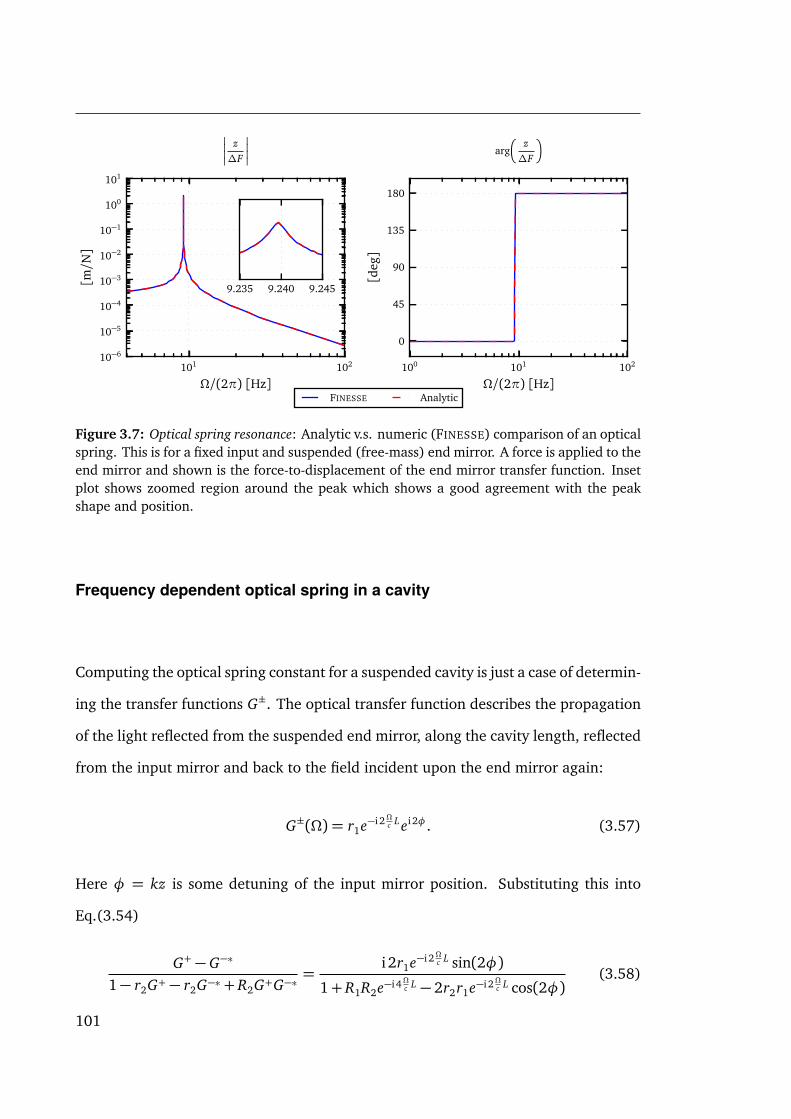
101 102
Ω/(2π) [Hz]
10−6
10−5
10−4
10−3
10−2
10−1
100
101
[m/N]
z∆F
9.235 9.240 9.245
100 101 102
Ω/(2π) [Hz]
0
45
90
135
180
[deg]
arg
z∆F
FINESSE Analytic
Figure 3.7: Optical spring resonance: Analytic v.s. numeric (FINESSE) comparison of an opticalspring. This is for a fixed input and suspended (free-mass) end mirror. A force is applied to theend mirror and shown is the force-to-displacement of the end mirror transfer function. Insetplot shows zoomed region around the peak which shows a good agreement with the peakshape and position.
Frequency dependent optical spring in a cavity
Computing the optical spring constant for a suspended cavity is just a case of determin-
ing the transfer functions G±. The optical transfer function describes the propagation
of the light reflected from the suspended end mirror, along the cavity length, reflected
from the input mirror and back to the field incident upon the end mirror again:
G±(Ω) = r1e−i 2Ωc Lei 2φ. (3.57)
Here φ = kz is some detuning of the input mirror position. Substituting this into
Eq.(3.54)
G+ − G−∗
1− r2G+ − r2G−∗ + R2G+G−∗=
i 2r1e−i 2Ωc L sin(2φ)
1+ R1R2e−i 4Ωc L − 2r2r1e−i 2Ωc L cos(2φ)(3.58)
101

3. OPTOMECHANICS
the optical spring constant is found:
κ(Ω) = −8kPc r1r2 sin(2φ)c
e−i 2Ωc L
1+ R1R2e−i 4Ωc L − 2r2r1e−i 2Ωc L cos(2φ). (3.59)
When the cavity is on resonance, φ = 0, we see no optical spring, likewise when there
is no power. Likewise, in the DC limit Ω→ 0 an agreement is found with Eq.(3.47).
Shown in figure 3.7 is and example of an optical spring force-to-displacement transfer
function of the suspended end mirror when a force is applied. It can also be seen in
Eq.(3.59) that imaginary component of κ, or optical damping, depends on the propa-
gation delay around the cavity.
3.1.5 The parametric gain: the measure of instability
Consider a mechanical mode of a mirror in some arbitrary interferometer, where the
optical field scattered by this mode produces an optical spring. The optical spring
differs slightly from Eq.(3.55) in that the scattering and force relations used are the
modal ones, Eq.(3.28) and Eq.(3.46). The equation of motion for the mode including
the optical feedback is
−MΩ2p = − κm(Ω)− κopt(Ω)
p+∆F(Ω), (3.60)
where the mechanical and optical spring terms are:
κm(Ω) = km + iΩcm, (3.61)
κopt(Ω) = kopt + iΩcopt(Ω). (3.62)
The combined response of the mode to both the optical and mechanical features
is κT = κm − κopt. This shifts the resonance frequency of the mode and alters the
102
damping ratio from the mechanical values:
ωT (Ω) =
√√km − kopt(Ω)
M, (3.63)
ωTγT (Ω) =ωmγm −ωopt(Ω)γopt(Ω), (3.64)
where ωopt(Ω) =Æ
kopt(Ω)/M . The various forms of damped harmonic oscillator are
applicable here: when γT > 1 the system is overdamped, γT = 1 it is critically damped
and γT < 1 it is underdamped. In the case where γT < 0 an initial oscillation grows
exponentially, thus the system is classed as unstable, or a parametric instability. To
parameterise this instability the parametric gain, R, is used [87]:
R(Ω)≡ ωopt(Ω)γopt(Ω)
ωmγm(3.65)
γT (Ω) =ωm
ωTγm(1−R(Ω)). (3.66)
When R > 1 the optomechanical coupling is unstable. Thus any small excitation of a
mode—be it from thermal, mechanical or optical—will grow overtime until the mode’s
amplitude is large enough to break the interferometer’s lock.
Extracting the parametric gain from transfer functions
Numerical tools such as FINESSE never explicitly calculate the optical spring constant
κopt, thus cannot simply outputR. However, they are an ideal tool for computing trans-
fer functions in which κopt and R appear and can be extracted from. A general method
for computing the parametric gain of a mode is outlined in [95]. Their method relies
on computing numerous optical transfer functions for each HOM field for the upper
and lower sideband. Such transfer functions could be extracted from the inverted in-
terferometer matrix but it would require a sparse solving of the interferometer matrix
for each HOM field in both the upper and lower sidebands. A more efficient method
103

3. OPTOMECHANICS
is outlined here which involves a single solution of the sparse matrix.
Using Eq.(3.60) we can compute transfer function:
p(Ω)∆F(Ω)
=1
κT (Ω)− MΩ2(3.67)
=1
M(ωT (Ω)2 + i 2ΩωT (Ω)γT (Ω)−Ω2)(3.68)
If a modal force is applied that produces a unit modal amplitude, for example ∆F =
∆p(Ω)/Hs(Ω):
p(Ω)∆p(Ω)
=ω2
m −Ω2 + i 2Ωγmωm
ωT (Ω)2 + i 2ΩωT (Ω)γT (Ω)−Ω2(3.69)
Inverting and computing the transfer function at Ω=ωm:
∆p(ωm)p(ωm)
=ωT (ωm)2 −ω2
m + i 2ωmωT (ωm)γT (ωm)
i 2γmω2m
(3.70)
Separating the real and imaginary parts and rearranging with Eq.(3.63) and Eq.(3.64):
∆p(ωm)p(ωm)
= 1−R(ωm) + ikopt
2M γmω2m
. (3.71)
The transfer function p(Ω)∆p(Ω) is a diagonal element in the inverted interferometer matrix
thus is easily extracted in a single sparse matrix solution at the mechanical frequency
ωm. Using Eq.(3.71), R can be efficiently extracted via the real part of the trans-
fer function. This process is encapsulated in the FINESSE parametric gain detector
pgaind. This can also form the basis of a detector which can output kopt produced
from the feedback of all optical modes if required.
The parametric instability code in FINESSE was validated against analytic calcu-
lations (which demonstrated good agreement bar some small numerical differences)
but also compared to the experimental results collected by Thomas Corbitt [89]. This
104

−1.0 −0.5 0.0 0.5 1.0
δ/γ
−4
−2
0
2
4
Para
met
ric
gain
,RFINESSE, Q_m=0.5·106
FINESSE, Q_m=0.75·106
FINESSE, Q_m=1·106
Experimental
Figure 3.8: Corbitt’s experimental PI comparison: Using data on the parametric instabilityexperiment conducted by Corbitt [89] a FINESSE model was constructed. The value δ/γ isthe detuning in units of the cavity linewidth. A mechanical drum head mode at 28.188kHz ispresent in the mirrors used, determined by their own FEM modelling. The data was extractedfrom figure 3 in the paper using a plot digitiser. Using the modal mass and optical parametersprovided in the work a reasonable fit of the data can be seen for the range of Q values thatwere expected for the drum head mode [96].
is one a few experiments aimed at measuring PI and radiation pressure effects. The
mechanical mode of interest in the experiment was the 28.188 kHz mechanical drum-
head mode of the mirror. This however can be approximated as just the longitudinal
motion of the mirror in our model as no strong optical scattering into modes higher
than TEM00 occurs. A simple FINESSE file was constructed for this experiment where
R is measured at various detunings of the cavity:
Code 3.1 FINESSE code to replicate Corbitt’s experiment
const PIfreq 28.188k
const mass 0.25
const Qm 1.5 M
l l1 3 0 n1
m1 Min 0.00631994 0 0 n1 n2
s cav1 1 n2 n3
m1 Mend 0 0 0 n3 dump
105

3. OPTOMECHANICS
# Page 98 in Corbitt ’s thesis mentions g ~ 0.8 Roc ~0.5 m
attr Min Rc -0.5125
attr Mend Rc 0.5125
# Add in masses and mechanical resonance of PI
tf susp 1 0 p $PIfreq $Qm
attr Mend m $mass zmech susp
cav c1 Min n2 Mend n3
maxtem 0 # Include up to order 0 optical modes
# Switch on the signal frequency calculations to compute
# parametric gain
fsig force $PIfreq
# Detect gain of longitudinal motion of mirror
pgaind Rz Mend z
xaxis Mend phi lin -0.09 0.09 1000
Exact details were not provided for all the parameters required, however most were
inferred from information in the paper and thesis [97]. Figure 3.8 shows the experi-
mental results overlaying the FINESSE output. The measured mechanical mode quality
factor is not explicitly stated in the paper or thesis, a value of Qm = 0.5− 1 · 106 [96]
though provided the fit depicted, which is not an unreasonable value.
3.1.6 Conditions for instability
As shown in Eq.(3.66) the optomechanical coupling of a mode becomes unstable if
the system becomes anti-damped, R > 1. Although this provides a convenient metric
to determined whether the mode is or is not stable it does not offer a clear physical
picture of the processes involved. A useful picture though is that of Stokes and anti-
Stokes scattering as originally used to described PIs in [87]. This describes the optical
106

scattering as the interaction of the photons in the carrier modes and the phonons of the
mechanical mode. The upper and lower sidebands are created when the photons in the
carrier field,ω0, interact with the phonons in the mechanical mode,ωm. The energy of
the photons in the upper and lower sidebands of the carrier are ħh(ω0±ωm). The lower
sideband photon has less energy than the carrier, thus to conserve energy when one
is created, a phonon must be too (this is known as the Stokes mode). When a carrier
photon and phonon are combined an upper sideband photon is created (the anti-
Stokes mode). When a lower sideband is produced energy is moved from the carrier
field into the mechanical mode. The opposite occurs when the upper sideband is
created; this is commonly referred to as optical cooling as energy is extracted from the
mechanical system. The likelihood of these scattering processes occurring depends on
whether the optical system can support scattered optical spatial and frequency modes.
If the photons of the lower sideband are resonant in the optical system the mechanical
mode is continuously pumped with energy from the carrier, greatly exciting the mode
and creating an instability.
These scattering processes are depicted in figure 3.9. The figure shows a contrived
setup for illustrating the point. Here a carrier field consisting of mostly TEM00 is reso-
nant in a cavity. There are then two mechanical modes present: one with a mechanical
frequencyωm1which scatters TEM00 into TEMnm, and the another with frequencyωm2
scattering TEM00 into TEMuv. In this scenario, and as depicted in figure 3.9, the lower
sideband created with frequency ωm1coincides with the mode separation frequency
of spatial mode TEMnm with which it primarily scatters into. The lower sideband sat-
isfies both the spatial and frequency constraints and is resonant. In this case the ωm1
could become unstable. Whether it does or not depends on the optical gain of from
the feedback. Note that the upper sideband for this mode is just off resonance, thus
a small amount of energy will be extracted from the mode, but not likely enough to
counteract the lower sideband. For the other mode we see the spatial and frequency
107
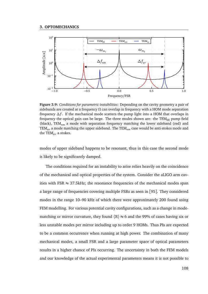
3. OPTOMECHANICS
−1.0 −0.5 0.0 0.5 1.0
Frequency/FSR
10−2
10−1
100
101
102
Am
plit
ude[a
.u]
∆ fnm ∆ fuv
−ωm1ωm2
TEM00 TEMnm TEMuv
Figure 3.9: Conditions for parametric instabilities: Depending on the cavity geometry a pair ofsidebands are created at a frequency Ω can overlap in frequency with a HOM mode separationfrequency ∆ f . If the mechanical mode scatters the pump light into a HOM that overlaps infrequency the optical gain can be large. The three modes shown are: the TEM00 pump field(black), TEMnm a mode with separation frequency matching the lower sideband (red) andTEMuv a mode matching the upper sideband. The TEMnm case would be anti-stokes mode andthe TEMuv a stokes.
modes of upper sideband happens to be resonant, thus in this case the second mode
is likely to be significantly damped.
The conditions required for an instability to arise relies heavily on the coincidence
of the mechanical and optical properties of the system. Consider the aLIGO arm cav-
ities with FSR ≈ 37.5kHz; the resonance frequencies of the mechanical modes span
a large range of frequencies covering multiple FSRs as seen in [95]. They considered
modes in the range 10–90 kHz of which there were approximately 200 found using
FEM modelling. For various potential cavity configurations, such as a change in mode-
matching or mirror curvature, they found ⟨R⟩ ≈ 6 and the 99% of cases having six or
less unstable modes per mirror including up to order 9 HOMs. Thus PIs are expected
to be a common occurrence when running at high power. The combination of many
mechanical modes, a small FSR and a large parameter space of optical parameters
results in a higher chance of PIs occurring. The uncertainty in both the FEM models
and our knowledge of the actual experimental parameters means it is not possible to
108

model exactly what modes would be problematic. However, as started in [95], a more
statistical outlook should be taken to estimate whether a particular interferometer
setup is likely or not to suffer from PIs [98].
3.2 Optical suppression of parametric instabilities
Thus far, modelling of parametric instabilities has been on searching for problematic
parameter spaces for aLIGO [99, 98, 100] for dual recycled interferometer. This pro-
cess has also begun for the Einstein Telescope [101, 102]. Potential mitigation of PIs
has also been theoretically and experimentally tested [103, 104]. These have pre-
dominantly involved using mechanical methods to suppress unstable modes such as
modulating the mirror mass using the thermal control system or applying dampeners
to the optics to change the resonant modes. Another technique applied in other fields
is that of optical cooling. This is achieved by pumping energy from the mechanical
mode into the optical field by making the upper sideband resonant within the sys-
tem. However, for the aLIGO arm cavities the resonances of the mechanical modes
are much higher than the cavity linewidth (≈ 80 Hz). Thus to cool the mode by mak-
ing the upper sideband is resonant would require detuning the arm cavity. This would
unacceptably reduce the sensitivity of the detector to gravitational waves and disturb
it whilst running in science mode. Thus such optical cooling cannot be applied in our
case.
However, little research has been conducted on controlling the PIs using purely op-
tical means. Suggestions have been made that specific optical HOMs could be shone
on to mirrors to dampening specific modes, which would rely on determining the un-
stable mode shape quickly and then injecting a suitable enough power level of the
HOM to dampen the mode. The question that I will answer here is whether it is possi-
ble to design an optical system where some control over the optical transfer functions
109

3. OPTOMECHANICS
ETMITM
IMC
ECM
Carrier scattered by mechanical mode
Telescope
Figure 3.10: Simple extraction cavity: The basic components required to extract HOMs froma cavity. This involves a mode cleaner to separate the TEM00 of the carrier field that will beresonant in the arm cavity and any HOM that are generated from PIs. An extraction cavity isthen formed with the reflection from the mode cleaner.
of the scattered fields can be exerted to reduce the parametric gain. Answering such
questions previously would have proven difficult as the necessary features of opti-
cal scattering, radiation pressure effects and optical transfer calculations for generic
systems did not exist in a complete and tested simulation tool. The work I have accom-
plished in FINESSE however now makes such studies possible. This section will focus
on exploring the idea of using two extra recycling mirrors for the HOMs reflected
from the IMC and OMC mirrors, as depicted in figure 3.23. The central idea is that
the resonance condition of the HOMs can be tuned in such a way to stop parametric
instabilities building up.
In this section I outline a simplified analytic description of the coupled cavity sys-
tem design and the general effects that arise. Next, I demonstrate that such a scheme
does in fact provide broadband reduction in the number of unstable PI.
3.2.1 Extraction cavities
The central idea that will be explored here for the suppression of parametric insta-
bilities is shown in figure 3.10. Here a coupled cavity arrangement is considered to
determine if such a configuration offers any potential for PI reduction in the arm cav-
110

Coupling Order |knm,00|Mode 37
00⇒ 01 1 0.1525800⇒ 03 3 0.043336500⇒ 21 3 0.024825100⇒ 00 0 0.0038649300⇒ 02 2 0.0011623300⇒ 20 2 0.0010133
Mode 140
00⇒ 11 2 0.083896400⇒ 13 4 0.054879100⇒ 10 1 0.0048158200⇒ 30 3 0.0024506400⇒ 12 3 0.0015206300⇒ 31 4 0.00103885
Table 3.2: The largest coupling coefficient terms (|knm,00| > 10−3) for scattering of TEM00into HOM from the mechanical mode 37 and 140 (See figure 3.4).
ities. It consists of three cavities: the arm cavity which is kept on resonance for the
TEM00 mode; an impedance matched input mode cleaner (IMC) tuned to filter the
incoming beam for the TEM00; and the extraction cavity, which is formed between
the input mirror of the arm and the extraction cavity mirror (ECM). The key aspect
here is that the extraction cavity forms a compound mirror for any fields that are not
transmitted through the IMC. When the IMC is tuned to transmit only the TEM00 of
the main carrier field, all of its higher order modes will be reflected. The extraction
cavity can then be designed to reduce the optical resonance condition for these fields
so that parametric gains can be reduced.
As discussed in the previous sections, a mechanical mode is excited in a mirror
when the spatial distribution of the radiation pressure exerted on the mirror surface
overlaps well with its shape. Such mechanical modes vary a great deal in shape; like
those shown in figure 3.4. The six largest spatial overlaps with optical modes up to
order four are shown in table 3.2. Here, it can be seen how much each optical mode
111

3. OPTOMECHANICS
ETMITMECM
Figure 3.11: Coupled cavity fields: To compute how a field injected into a coupled cavitysystem resonates the shown fields need to be considered. Here a0 is some mode created in thecavity. The field incident on the ITM a1 is reflected into a2 as usual. However, in this case thefield also circulates in the extraction cavity a3 which then transmits back through to the armcavity.
contributes to the excitation of these two mechanical modes, thus lists which modes
would need to be suppressed.
Other mechanical modes will have different unique combinations of modes. In
reality the mechanical mode shapes are not exactly known and will depend on nu-
merous experimental factors, such as the temperature of the mirror and differences
in construction. Thus which mechanical modes will actually become unstable is not
known exactly.
For optical suppression to be of much use, an optical layout that suppresses all the
higher order modes must be found. Suppressing a single optical mode shape will not
suffice, as another mode may also become unstable due to a different set of modes.
There is also the issue that the resonant frequencies of the mechanical modes are
fairly well distributed in frequency above ≈ 10 kHz. If a particular mode TEMnm
happens to overlap well with a mechanical mode at both 20 kHz and 50 kHz, a setup
must be constructed to suppress the fields at both frequencies. This is a particularly
important criteria as the FSR of future generation interferometers are of the same
order of frequencies as the mechanical modes: 37.5 kHz for LIGO and 15 kHz for ET.
112

Extraction cavity design
Firstly, it will be analysed how an optical mode resonates in a simplified coupled cavity
system. In particular an understanding of how any TEMnm mode of the lower sideband
resonates, as this results in energy being pumped from the main carrier field into the
mechanical mode. To compute the intracavity field in the arm the extraction cavity
is treated as a compound mirror. The analytic model considered here is shown in
figure 3.11. This simplified model assumes the mode cleaner used to separate the
higher order modes from the main TEM00 of the carrier is operating perfectly, thus
can be ignored in the analytics. The intracavity field in the extraction cavity is given
by
a3 = a1i t2r3
1− r2r3G2. (3.72)
Here G2 is the propagator for the scattered field around the extraction cavity being
considered. For a higher order mode this will be
G2 = exp
i
2ΩL2
c+ (n+m)Ψrt,2 + 2φ
. (3.73)
Here Ψrt,2 is the round-trip Gouy phase and φ is any tuning of the extraction cavity
mirror: setting φ = 0 here ensures that the TEM00 is resonant. The extraction cavity
then alters the reflectivity of the input mirror from the point of view of a field incident
from the arm cavity:
a2 = r2a1 + i t2a3, (3.74)
a2
a1= r2 −
T2r3G2
1− r2r3G2=
r2 − r3G2(R2 + T2)1− r2r3G2
, (3.75)
113

3. OPTOMECHANICS
which is assuming the mirrors are lossless R2 + T2 = 1. Given some initial excitation
of the mode of interest in the arm cavity, a0, the cavity field is then
a1 =a0
1− r1G1
r2 − r3G2
1− r2r3G2
. (3.76)
Here G1 is the propagator for the field around the arm cavity. Eq.(3.76) describes how
a mode created in the arm cavity resonates within it. The power in this field is
|a1|2 =|a0|2|1− r2r3G2|2
|1− r2r3G2|2 + R1 |r2 − r3G2|2 − 2r1 Re
G1(r2 − r3G2)(1− r2r3G∗2) . (3.77)
Note that the relative phase, thus where in the cavity it was created, of the mode
does not factor into the resonance condition. The actual magnitude of a0 will be
determined by the scattering matrix for a particular mechanical mode, this merely
complicates the equations with no benefit at this stage. It is also assumed that the end
mirror is perfectly reflective, R1 ≈ 1; as is the case for arms cavities in the gravitational
wave detectors.
Extraction cavity length
Expanding Eq.(3.77), the circulating power for an excited mode in the arm cavity is
|a1|2 = |a0|21+ R2R3 − 2r2r3 cos(∠G2)
(R2 + 1)(R3 + 1)− 4r2r3 cos(∠G2)− 2r2(1+ R3) cos(∠G1) . . .+ 2r3[cos(∠G1 +∠G2) + R2 cos(∠G1 −∠G2)]
. (3.78)
= |a0|2SD
, (3.79)
where S is the suppression factor and D the denominator of the above expression.
Here D describes how the mode will resonate in the coupled cavity system. How the
resonances behave is analysed later in this section. Ideally for every resonance of the
mode as determined by D there should be an equivalent minimum in S to suppress it.
114

0 2 4 6 8 10 12 14
FSR
10−2
10−1
100
L2/L1 = 0.013
0 2 4 6 8 10 12 14
FSR
10−2
10−1
100
L2/L1 = 0.25
No extraction cavity With extraction cavity
0 2 4 6 8 10 12 14
FSR
10−2
10−1
100
L2/L1 = 1
Figure 3.12: Long vs short extraction cavity suppression: Using Eq.(3.78) the effect of theextraction cavity on the resonance of an optical field in the arm cavity can be seen. This isshown for different extraction cavity lengths. For equal lengths the resonance of the field issuppressed for multiple FSRs, the ideal scenario. For shorter lengths the resonance conditionof the extraction suppresses some FSRs but for others increases it. The next preferable caseis where the extraction cavity is very short compared to the arm cavity length. In this casethe length can be chosen to suppress up to the 10th FSR, using a length ratio determined withEq.(3.82).
Here S depends purely on the resonant condition of the mode within the extraction
cavity; which is minimised when the mode is resonantly enhanced, ∠G2 = 2Nπ. By
exploring the parameter space of various cavity length ratios, L2/L1, two scenarios
were found to be promising: an extraction cavity whose length is some positive and
non-zero integer of the arm length, L1 = L2; and an extraction cavity length which is
much less than the arms, L2 L1.
Using an integer ratio of cavity lengths allows the setup to suppress the resonance
of a mode at each of its FSRs, as shown in figure 3.12. This is because the FSR of
both the arm and extraction cavity are the same. From a practical perspective, as
the arm cavity’s lengths are already long, having a second cavity even longer is not
particularly desirable. However, one that is the same length could in theory be housed
within shared vacuum tubes and facilities.
In this case where L2 L1, the bandwidth of the extraction cavity is large enough
to encompass multiple FSRs of the arm cavity and suppress them. However, eventu-
115

3. OPTOMECHANICS
ally an FSR will be reached where they are no longer suppressed and the resonances
become enhanced, such as shown in figure 3.12. The maximum number of FSRs that
require suppressing will depend on both the length of the arm cavity (as longer arms
means a smaller FSR) and the frequency distribution of the mechanical modes over
multiple FSRs present in the mirrors. Once the maximum number of potentially un-
stable FSRs are known the required length ratio can be computed.
To determine the length ratio required to suppress up to a chosen N thFSR FSR, the
resonance of the mode without an extraction cavity (r3 = 0) is compared to one with.
From this comparison we can see for a given length ratio how much a particular FSR
is suppressed. Using Eq.(3.78) to make the comparison,
1D|r3=0
=SD
. (3.80)
we want to solve this for ∠G2, which contains the extraction cavity length: ∠G2 =
4π f L2/c. As the suppression of mode on resonance is desired, the frequency will be
some integer number of FSRs f = NFSR FSR. The FSR in this case being that of the
arm cavity, FSR = c/(2L1). This results in ∠G1 = 2NFSRπ. By solving Eq.(3.80) and
substituting in the above statements, it is found that
∠G2 =4π f L2
c= 2πNFSR
L2
L1= cos−1
r3(r2 − 1)
2
. (3.81)
Finally, the length ratio that is required to suppress up to the N thFSR FSR resonance must
satisfyL2
L1<
12πNFSR
cos−1
r3(r2 − 1)2
® 1
4NFSR. (3.82)
The approximated version is valid when a high reflectivity ITM is used (r2 ≈ 1). An
example of this is shown in the first subplot of figure 3.12. Here it was chosen to
suppress up to the 10th FSR. Obviously if the last FSR requires a reasonable amount
116

of suppression the ratio must be lowered further. The current design in aLIGO has
≈ 60 m from the ITM to the IMC which means up to the 16th FSR could in theory be
suppressed.
Extraction cavity mirror reflectivity
The next design choice for the extraction cavity is the reflectivity of the extraction
cavity mirror (ECM). Choosing the reflectivity simply enables more or less of the light
reflected from the mode cleaner to be recycled back into the arm to suppress the mode.
It will be shown that the reflectivity of the ECM can produce two different behaviours
of the system: of which I will refer to as the weak and strong coupling regimes.
In the weak coupling regime a mode is resonant at a single frequency. In the strong
coupling regime a frequency split occurs and the mode will resonate at two distinct
frequencies. Such resonance information could be extracted from the denominator of
Eq.(3.78): where the differential cosines of G1 ± G2 suggest a splitting could occur.
However, extracting such information about the resonant frequencies in this form is
not particularly clear.
Performing an eigenvalue analysis of the system allows us to determine the linewidth
and resonant frequencies of the system; the real part of the eigenvalue gives the res-
onant frequency and the imaginary the linewidth. This would involve solving the
coupled differential wave equations for the field in both cavities. However, this step is
greatly simplified as we already have the solutions to waves propagating in the cavities
using our steady-state formalism. The coupled cavity system is described by just two
coupled equations:
a1 = a3i t2r1G1
1− r1r2G1= a3A, (3.83)
a3 = a1i t2r3G2
1− r2r3G2= a1B. (3.84)
117

3. OPTOMECHANICS
0.0 0.2 0.4 0.6 0.8 1.0
Reflectivity, R3
−800
−600
−400
−200
0
200
400
600
800
Freq
uenc
y[H
z]
Ω+eq
Ω−eq
0.0 0.2 0.4 0.6 0.8 1.0
Reflectivity, R3
10−1
100
101
102
103
104
105
Line
wid
th[H
z]
Ω+eq
Ω−eq
Figure 3.13: Coupled cavity frequency split: Using Eq.(3.87) the frequency splitting can beseen for an aLIGO like cavity. As the reflectivity reaches the critical value two resonances arethen seen and separate further. The linewidth then decreases rapidly, this will correspond toa much higher gain at the particular resonances but the thinner linewidth provides greatersuppression of the mode at other frequencies.
The characteristic equation of the system is found with
det
1 −A
−B 1
= 0, (3.85)
which, after expanding, means solving for Ω in
r1r2 exp (−2i L1Ω/c) + r2r3 exp (−2i L2Ω/c)− r1r3 exp (−2iΩ[L1 + L2]/c) = 1. (3.86)
In general there is not an analytic solution for Ω here.
In the case of coupled cavities with equal lengths Eq.(3.86) can be solved for Ω
directly:
Ω±eq = −i c
2πL1loge
√√√ r1r2 + r2r3 ±
pR1R2 + 2R2r1r3 − 4r1r3 + R2R3
2
. (3.87)
These solutions can be seen in figure 3.13 for an aLIGO like cavity ( r1 = 1, r2 =p
0.986, L1 = 3994.5 m). Here the splitting can be clearly seen when the extraction
cavity reflectivity is increased beyond a critical reflectivity, which is denoted as Rc. Be-
118

fore this stage there are two resonances at the same frequency, one with an increasing
linewidth and one with a decreasing linewidth. The eigenvalues in this regime are
purely imaginary as we are looking at the 0th FSR resonance, which is defined relative
to 0 Hz. At the critical reflectivity the two resonances split, with a linewidth tending
to 0 Hz with R3 = 1.
The frequency split occurs when the log term in Eq.(3.87) becomes complex, before
this we are left with a purely imaginary value. This occurs when the inner square root
becomes negative. Solving the quadratic equation for r3 provides two solutions, one
gives r3 > 1 which is ignored, the other providing the critical reflectivity for equal
length coupled cavities:
Reqc =
2− R2 − 2
p1− R2
R22
2
. (3.88)
The maximum frequency separation is found by taking the limit of r3→ 1, which gives
f eqsp =
c4πL1
tan−1
t2
r2
≈ c t2
4πL1. (3.89)
When the lengths are equal this frequency splitting applies to all of the FSR resonances.
This is because Ω±eq + NFSR FSR is also a solution to Eq.(3.86) for any integer NFSR.
In the case where the cavities are not of equal length numerous approximations
must be made to find reasonable solutions for Ω in Eq.(3.86). The maths undertaken
here was done using a symbolic math package. Here a second order expansion in
terms of Ω for the exponentials is used. A second order expansion is required as two
solutions will be present, one for both the positive and negative frequency split. With
a small length ratio, the frequency splitting will only occur around FSRs which match
between both the arm and extraction cavity.
For the cavities of interest for GW detectors it is also assumed that r1 ≈ 1, r2 =p
1− T2 ≈ 1 − T2/2 for small T2, the length ration is also parameterised with L2 =
119

3. OPTOMECHANICS
−3 −2 −1 0 1 2 3
FSR
10−2
10−1
100
101
102
103∆L = 0.1
−3 −2 −1 0 1 2 3
FSR
10−2
10−1
100
101
102
103∆L = 0.5
No extraction cavity With extraction cavity
−3 −2 −1 0 1 2 3
FSR
10−2
10−1
100
101
102
103∆L = 1
Figure 3.14: Frequency split vs. cavity lengths: Shown are the resonances of a mode overfrequency in the arm cavity for different length ratios. The extraction cavity mirror is perfectlyreflective in this case to highlight the frequency splitting. For short length ratios only the 0th
FSR is affected by the splitting, for equal lengths each FSR is split. The splitting occurs whenthe resonance of the extraction cavity is aligned with a resonance in the arm, as given byEq.(3.78).
∆L L1; where ∆L ® 1. Expanding and solving Eq.(3.86) provides a second order poly-
nomial in Ω. Its determinant of this polynomial controls when the frequency split
occurs. Finding the determinant and solving for r3 the critical reflectivity for such a
system is found to be
Rc =
T2(1− 3∆L)− 2+
ÆT 2
2 (9∆2L − 6∆L + 1) + 16∆L T2
2(T2∆L + T2 − 1)
2
. (3.90)
The maximum frequency split can be approximated by taking the limit of r3 → 1.
Taking this limit and removing negligible terms the maximum frequency split is
f ±sp ≈ ±cÆ
3T 22 + 16T2∆L
4πL1(T2 + 4∆L). (3.91)
It can be seen that fsp increases with smaller length ratios. For small ∆L < 0.1
Eq.(3.91) the original second order expansion of the exponentials is no longer valid
for larger frequencies. However using Eq.(3.86) with similar approximations of small
120

T2 but considering the limits ∆L → 0 and r3→ 1 the separation tends to value:
f ±sp ≈ ±c
4L1, (3.92)
which is just half the FSR of the arm cavity. With this frequency offset we no longer
have two distinct resonances, as the current and next FSRs positive and negative split-
ting merge into one. Thus with small the resonances of the cavity can be seen as just
shifted in frequency by FSR/2. This was numerically experimented with and found to
apply for ∆L ® 10−3.
This subsection has outlined the behaviour of the optical resonances in an equal
and short length ratio coupled cavity system analytically. A mechanical mode becom-
ing unstable will only be problematic if it coincides at frequencies where there is also
an optical resonance in the system. These formulae show how these resonances be-
have with respect to multiple variables which can be difficult to extract concisely from
numerical simulations. This also helps better understand the numerical results and
demonstrate such code is working as expected. The discussion of pros and cons of
each regime is discussed in section 3.2.1 where the numerical results are also pre-
sented.
Extraction cavity stability
The final design choice regarding the extraction cavity is its geometric stability, or the
amount of round-trip Gouy phase accumulated. This must be chosen to ensure that
modes of differing orders are suppressed for the same extraction cavity tuning. If this
is not the case the suppression of one mode will most likely coincide with an additional
excitation of another. A mode circulating in the extraction cavity will accumulate some
Gouy phase dependent on its order and some additional mode independent phase from
any cavity detuning, which is represented by an ECM tuning of φ. The round-trip
121
3. OPTOMECHANICS
phase accumulated is then:
∠G2,nm =2ΩL2
c+ (n+m)Ψrt,2 + 2φ, (3.93)
For the TEMnm mode to be resonant ∠G2,nm = 2Nπ. This is only possible for any
order of HOM if Ψrt,2 ≈ π, or in other terminology, the extraction cavity is unstable.
To achieve this Gouy phase whilst simultaneously ensuring the above length ratio
requirements an extraction mirror telescope will have to be designed. The actual
design, whether this involves lenses or mirrors, is not considered here. The models
used will force the accumulated Gouy phase a long a space to have the required value.
To summarise, an extraction cavity can be designed to feedback fields other than
the TEM00 of the carrier to suppress the resonant build up of such fields. This can be
achieved for multiple FSRs and HOMs at the same time using an unstable extraction
cavity. The reduced amount of HOM optical fields should in theory reduce the optical
feedback via radiation pressure that drives mechanical modes to instability. Thus far
only simplified analytics has been shown for the optical fields in a coupled cavity
system. To demonstrate the following section will apply this theory in a numerical
experiment to demonstrate its workings.
3.2.2 Numerical experiment
The numerical experiments conducted here are all done using the aLIGO IMC and
arm cavity design. These are combined as shown in figure 3.10. Some additional
lenses are required between the IMC and cavity to mode match the pair. To do this an
optimisation routine was employed to maximise the circulating cavity power whilst
varying each of the lens’ position and focal length. A mode matching setup was found
such that the circulating power differed by 1ppm compared to the plane wave case—
where mode-matching is not considered. The actual values of the lens and their po-
122
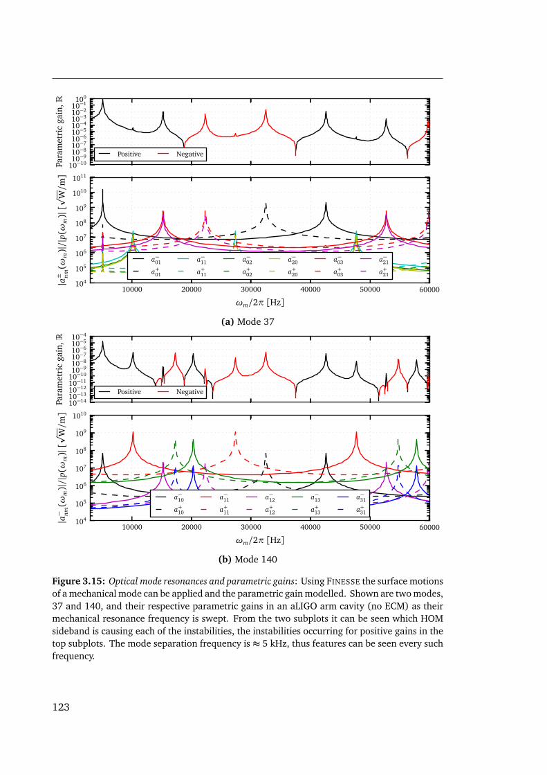
10−1010−910−810−710−610−510−410−310−210−1100
Para
met
ric
gain
,R
Positive Negative
10000 20000 30000 40000 50000 60000
ωm/2π [Hz]
104
105
106
107
108
109
1010
1011
|a± nm(ω
m)|/|p(ω
m)|[p
W/m]
a−01
a+01
a−11
a+11
a−02
a+02
a−20
a+20
a−03
a+03
a−21
a+21
(a) Mode 37
10−1410−1310−1210−1110−1010−910−810−710−610−510−4
Para
met
ric
gain
,R
Positive Negative
10000 20000 30000 40000 50000 60000
ωm/2π [Hz]
104
105
106
107
108
109
1010
|a− nm(ω
m)|/|p(ω
m)|[p
W/m]
a−10
a+10
a−11
a+11
a−12
a+12
a−13
a+13
a−31
a+31
(b) Mode 140
Figure 3.15: Optical mode resonances and parametric gains: Using FINESSE the surface motionsof a mechanical mode can be applied and the parametric gain modelled. Shown are two modes,37 and 140, and their respective parametric gains in an aLIGO arm cavity (no ECM) as theirmechanical resonance frequency is swept. From the two subplots it can be seen which HOMsideband is causing each of the instabilities, the instabilities occurring for positive gains in thetop subplots. The mode separation frequency is ≈ 5 kHz, thus features can be seen every suchfrequency.
123

3. OPTOMECHANICS
sitions are not of much importance here as this just ensures that any effects from
mode-mismatches are minimised. The length between the IMC and arm containing
the lenses though was kept as short as possible, thus allowing for shorter length ratios
for the extraction cavity. This setup is then able to pump the arm with TEM00 laser
and various surface motions can be applied to study any unstable modes.
The modes used were generated using COMSOL as discussed in earlier sections. In
all around 800 mechanical modes were computed ranging from≈ 1–60 kHz. The data
for theses modes can be found in the aLIGO FINESSE Git repository [29], for those that
are interested in performing similar simulations. For each of the mechanical modes
the surface motion is extracted and converted into a format that FINESSE can read.
The maps are then further processed to enabled reduced order quadrature as outlined
in chapter 2 to greatly speedup the scattering matrix calculations. Here 800 maps will
need to be run, without ROQ the runtimes would be excessively long.
To illustrate the behaviour of the two modes the surface motions can be applied in
FINESSE using the setup depicted in figure 3.10, but with no ECM to begin with. The
mechanical frequency of each mode is swept over an FSR to see where the mechanical
modes are excited or damped. For each frequency the mechanical mode is excited by
computing how much of each sideband is generated for a unit motion of the surface,
then along with this the parametric gain is calculated. The results of this scan for the
two modes 37 and 140 are shown in figure 3.15. Enough higher order modes were
used to capture the main features from the scattering, which was up to order four for
these particular modes. Comparing the resonances to table 3.2 the largest coupling
coefficients match with the resonances seen in the figure. It should be noted that
by sweeping a mode’s mechanical frequency like this we can find which frequencies
would be problematic. If in reality the mode were to have a frequency that lies near a
positive gain peak, it would then have the potential to become unstable. The respective
resonance frequencies for mode 37 and 140 as computed by COMSOL are ≈ 15.5 kHz
124

and ≈ 28.5 kHz. It can be seen here that mode 37 lies close to a positive 15 kHz
peak for the order three modes which is strongly couples with, thus is a candidate for
potential instability. Mode 140 however lies close to a negative gain peak thus is not
problematic.
The uncertainty of any given mechanical modes computed frequency compared to
its real frequency is a considerable obstacle for computing exactly which mode will be
unstable. Work has been previously done on comparing 3D FEM tools ability to com-
pute a resonant mode compared to theoretical predictions for a cylindrical mass [105].
Here, it was shown that the accuracy depends strongly on the computational method
applied, in some cases the computed value being ≈ 102 Hz off for higher frequencies.
Since writing this there are no procedures that can be used to test the accuracy of the
COMSOL modes generated that have been used for this work. However, entirely ac-
curate frequencies are not of importance here as a general suppression of mechanical
modes is being studied; a reasonable collection of varied mode shapes and frequency
distribution to study if all are suppressed. With no better determinant for whether a
mode could become unstable, I will class one as having the potential to become unsta-
ble if a positive gain peak with R > 1 exists within ±2 kHz of the COMSOL resonant
frequency; a similar range was used in [106].
3.2.3 Results of PI suppression with the ECM
Including the ECM in the numerical model the effect on the mechanical modes can
be studied. Two setups were constructed for equal and short (∆L ≈ 0.01) length
ratios. The setup was mode well mode matched for both by carefully tuning the lenses
and lengths between the IMC and arm cavity. In the equal length case the effect
the ECM reflectivity has can be seen in figure 3.16. Here, the mechanical frequency
of the mode is scanned whilst looking at how the parametric gain is affected. This
clearly demonstrates the coupled cavity frequency splitting as discussed analytically:
125
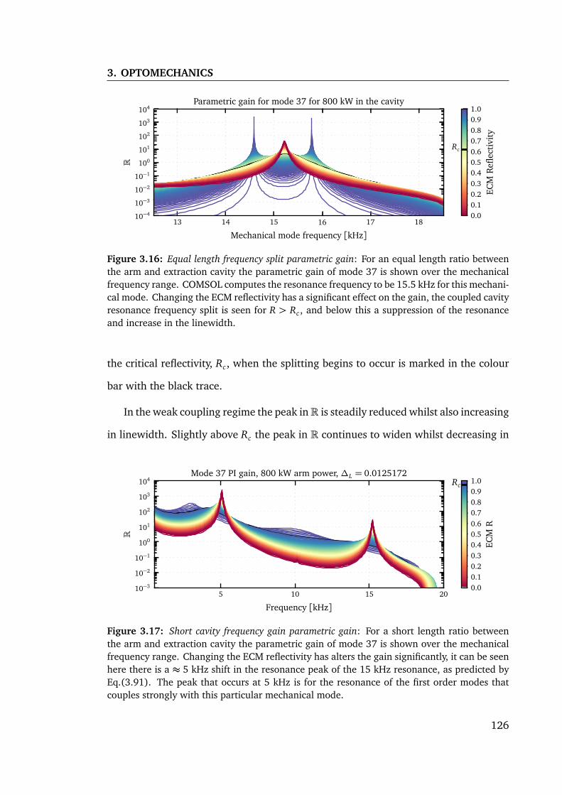
3. OPTOMECHANICS
13 14 15 16 17 18
Mechanical mode frequency [kHz]
10−4
10−3
10−2
10−1
100
101
102
103
104
R
Parametric gain for mode 37 for 800 kW in the cavity
0.00.10.20.30.40.50.60.70.80.91.0
ECM
Refl
ecti
vity
Rc
Figure 3.16: Equal length frequency split parametric gain: For an equal length ratio betweenthe arm and extraction cavity the parametric gain of mode 37 is shown over the mechanicalfrequency range. COMSOL computes the resonance frequency to be 15.5 kHz for this mechani-cal mode. Changing the ECM reflectivity has a significant effect on the gain, the coupled cavityresonance frequency split is seen for R > Rc , and below this a suppression of the resonanceand increase in the linewidth.
the critical reflectivity, Rc, when the splitting begins to occur is marked in the colour
bar with the black trace.
In the weak coupling regime the peak inR is steadily reduced whilst also increasing
in linewidth. Slightly above Rc the peak in R continues to widen whilst decreasing in
5 10 15 20
Frequency [kHz]
10−3
10−2
10−1
100
101
102
103
104
R
Mode 37 PI gain, 800 kW arm power, ∆L = 0.0125172
0.00.10.20.30.40.50.60.70.80.91.0
ECM
RRc
Figure 3.17: Short cavity frequency gain parametric gain: For a short length ratio betweenthe arm and extraction cavity the parametric gain of mode 37 is shown over the mechanicalfrequency range. Changing the ECM reflectivity has alters the gain significantly, it can be seenhere there is a ≈ 5 kHz shift in the resonance peak of the 15 kHz resonance, as predicted byEq.(3.91). The peak that occurs at 5 kHz is for the resonance of the first order modes thatcouples strongly with this particular mechanical mode.
126

13 14 15 16 17 18
Mechanical mode frequency [kHz]
10−6
10−5
10−4
10−3
10−2
10−1
100
101
102
103
R
Parametric gain for mode 37 for 800 kW in the cavity, ECM R3 = 0.95
−20−16−12−8−4048121620
ECM
tuni
ng[d
eg]
Figure 3.18: Equal length extraction cavity tuning: For an equal length ratio between the armand extraction cavity the parametric gain of mode 37 is shown over the mechanical frequencyrange as the ECM is detuned but with a reflectivity of 0.95.
maximum gain before the split resonances become visible. At perfect ECM reflectivity
there exists two narrow high gain peaks corresponding to the new optical resonances
of the system. It can be seen in this case that it is essentially impossible to completely
remove all instabilities. However, the parametric gain can be shaped.
The ideal choice of ECM reflectivity is perhaps not straightforward. By using a low
R we reduce the original peak’s maximum gain without introducing further peaks. Yet
the broadening of this peak, resulting in more frequencies where R > 1, means that
the probability of a mechanical mode finding itself in an unstable frequency range
is increased, thus more PIs could exist. Operating with a very low ECM reflectivity
whilst keeping the linewidth small does offer a slight reduction in R, but such a small
change would add additional experimental complexity with more mirrors to control
whilst offering little suppression of any unstable modes.
If the broadening of the peaks are thought not to be an issue, the ideal choice would
be a reflectivity slightly higher than Rc; here the resonance is split but the linewidth
of the two merge into an overall wider peak with a lower maximum gain.
The other option is to use the highest reflectivity possible. With this the frequency
split in the resonances have much higher peak gains but with much smaller linewidth.
127

3. OPTOMECHANICS
13 14 15 16 17 18
Mechanical mode frequency [kHz]
10−4
10−3
10−2
10−1
100
101
102
R
Parametric gain for mode 37 for 800 kW in the cavity, ECM R3 = 0.5
−15−12−9−6−303691215
ECM
tuni
ng[d
eg]
Figure 3.19: Short extraction cavity tuning: For short length ratio between the arm and ex-traction cavity the parametric gain of mode 37 is shown over the mechanical frequency rangeas the ECM is detuned but with a reflectivity of 0.5.
This would reduce the probability that a mechanical frequency would coincide with
an optical frequency having R, therefore may be a preferable option. Such a narrow
linewidth also has the benefit that only small changes in parameters would be needed
to shift the resonance frequency of the mode to stop one from being unstable.
Performing the same analysis for the short length ratio the parametric gain behaves
as seen in figure 3.17. Here, we do not see any frequency splitting as demonstrated
in the analytics. The gain is shown over a larger range here to show how the large
frequency shift, ≈ 5 kHz, as predicted by Eq.(3.91) effects R. Around the actual
mechanical resonance frequency, 15.5 kHz, the gain is significantly reduced.
The effect of detuning the extraction cavity shifts the resonance peaks. For high
reflectivities as seen in figure 3.18 the direction of the detune decides whether the up-
per or lower resonant mode is shifted in frequency. Like the use of the thermal control
system to shift the mechanical resonance mode, the ECM detuning offers a method
to shift which optical frequency is resonant; if a PI was seen to be ringing up then it
could be possible to detune the extraction cavity to stop the PI building up further.
The only problematic aspect here is that this detuning will affect all optical modes,
which could result in other optical modes then becoming co-resonant with mechani-
128

cal modes inducing further instabilities. Detuning in the weak coupling regime as seen
in figure 3.19 shifts the peak up or down in frequency whilst increasing the maximum
gain. Thus again offering a method for shifting where the largest PI gain is.
Shown in figure 3.20 is the effect that detuning has on mode 37 and 140. For this
the largest maximum around 15.2 kHz and 10.2 kHz for each mode respectively is
tracked with a peak finder as the ECM is tuned. The top plot shows the dominant op-
tical modes in the lower sidebands resonant in the arm cavity as the mechanical mode
is excited. As expected when the EC is tuned to suppress these, R is at a minimum.
Shown also is the position of the maximum gain, which varies greatest around the
minimum. For these results the Gouy phase of the EC was not tuned to demonstrate
how the minimum R occurs for different EC detunings.
The Gouy phase accumulated between the IMC and ECM was tuned to ensure that
π Gouy phase is accumulated between the ITM and ECM in the model, thus ensur-
ing the suppression of each mode. By choosing the EC Gouy phase and its tuning
correctly it was possible to suppress any PI that appeared for any mechanical mode.
The numerical experiment took each of the 800 mechanical modes and computed the
maximum parametric gain in the frequency range ±2 kHz around the COMSOL com-
puted resonance mode. This additional range was chosen rather arbitrarily but is to
take into account some uncertainty in what exactly the mechanical modes resonance
is. These numerical experiments were then ran for multiple ECM reflectivities of equal
length coupled cavity system. Similar results were seen for a short length ratio sys-
tem where equation 3.82 was used to ensure all modes in the frequency range were
suppressed. In the short case there was also an absence of frequency splitting seen at
high frequencies as demonstrated in figure 3.12.
This analysis was first applied to mechanical modes on the ETM, the results of
which are shown in figure 3.21. Here each point represents a positive R peak. With
800 kW of power in the arm cavity and no extraction cavity 115 modes were found to
129

3. OPTOMECHANICS
−100 −50 0 50 100
PREM tuning [deg]
103
104
105
106
107
108[p
W/(
pPci
rc)]
Magnitude of lower sideband per unit of mechanical mode motionand per Watt of circulating power for mode 37
TEM03 PREMTEM21 PREMTEM03 ArmTEM21 ArmTEM03 IMCTEM21 IMC
−100 −50 0 50 100
PREM tuning [deg]
0.00
0.05
0.10
0.15
0.20
0.25
MaxR[1/k
W]
Max R per kW of circulating power
−100 −50 0 50 100
PREM tuning [deg]
15.0515.1015.1515.2015.2515.3015.35
ωm/2π[k
Hz]
ωm/2π for max R
(a) Mode 37
−100 −50 0 50 100
PREM tuning [deg]
104
105
106
107
108
Fiel
d[p
W/(
pP c
irc)]
Magnitude of lower sideband per unit of mechanical mode motionand per Watt of circulating power for mode 140
TEM11 PREMTEM11 armTEM11 IMC
−100 −50 0 50 100
PREM tuning [deg]
0123456789
MaxR[1
0−6/k
W] Max R per kW of circulating power
−100 −50 0 50 100
PREM tuning [deg]
10.0010.0510.1010.1510.2010.2510.30
ωm/2π[k
Hz]
Mechanical frequency of max R
(b) Mode 140
Figure 3.20: Two mechanical modes and an extraction cavity: The two modes shown in fig-ure 3.4, modes 37 and 140, were placed in the extraction cavity setup shown in figure 3.10.The effect on the HOM of the lower sideband can be see in the upper subplots as the ECM isdetuned. As the ECM is detuned a peak finder records the maximum gain and its position; theeffect of which is shown in the lower subplots. As can be seen the lower circulating opticalmodes that coupled strongly with the mechanical mode corresponds to a lower parametricgain.
130

0 10 20 30 40 50 60
Frequency [kHz]
10−1
100
101
102
R
ETM parametric gains, with 800 kW
0102030
Nu
ECM R=0, total unstable modes = 115
0
4
8
Nu
ECM R=0.5, total unstable modes = 38
0
4
8
Nu
ECM R=0.75, total unstable modes = 26
0 10 20 30 40 50 60
Frequency [kHz]
0102030
Nu
ECM R=0.95, total unstable modes = 126
Figure 3.21: ETM parametric instability reduction: Applying the 800 mechanical modes to thearm’s ETM mirror in the extraction cavity setup its ability to suppress multiple modes can beseen. Each data point relates to a specific mechanical mode that has a positive parametricgain peak within ±2 kHz of its COMSOL computed resonance frequency. Here the varyingreflectivities of an equal length ratio setup clearly shows a reduction in the peak parametricgain across the full range of modes tested. The FSR of the cavity is ≈ 37.5 kHz so we also seea multiple FSR reduction too.
131
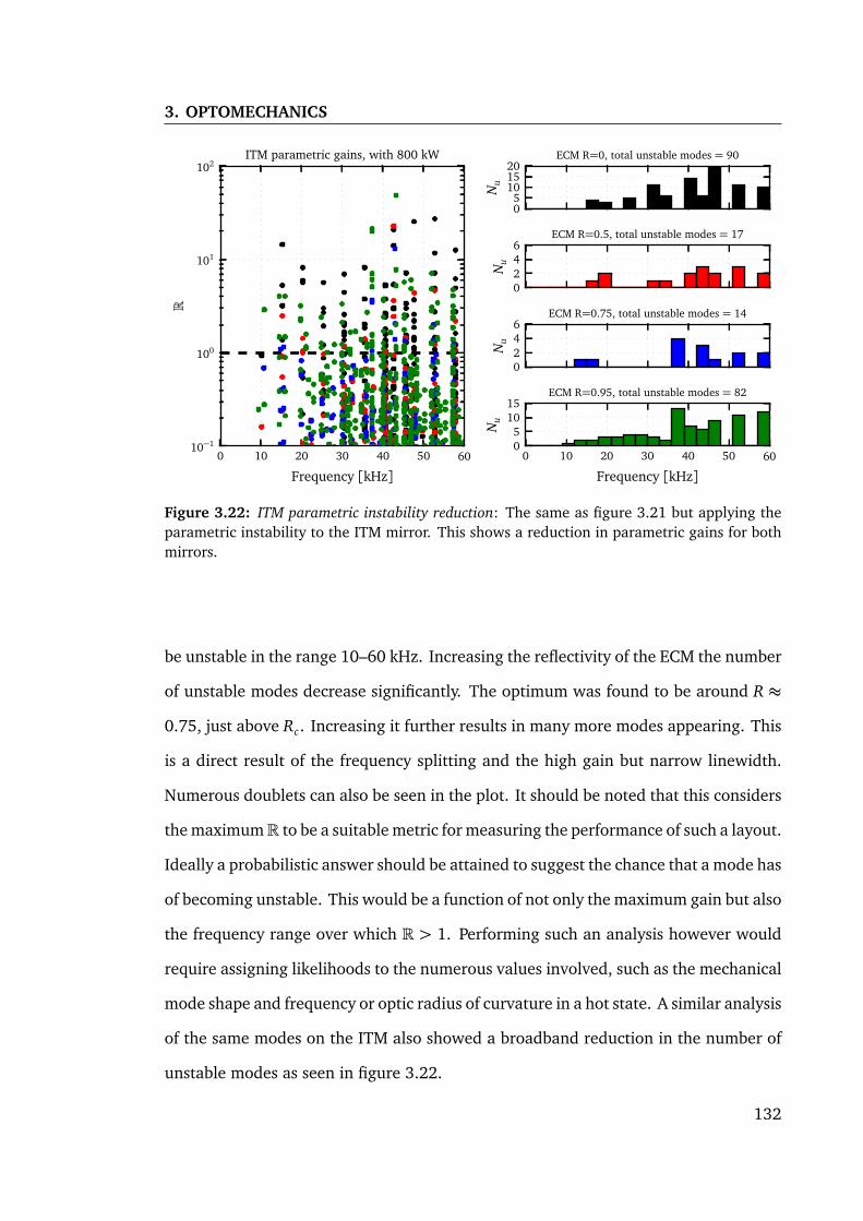
3. OPTOMECHANICS
0 10 20 30 40 50 60
Frequency [kHz]
10−1
100
101
102
RITM parametric gains, with 800 kW
05
101520
Nu
ECM R=0, total unstable modes = 90
0246
Nu
ECM R=0.5, total unstable modes = 17
0246
Nu
ECM R=0.75, total unstable modes = 14
0 10 20 30 40 50 60
Frequency [kHz]
05
1015
Nu
ECM R=0.95, total unstable modes = 82
Figure 3.22: ITM parametric instability reduction: The same as figure 3.21 but applying theparametric instability to the ITM mirror. This shows a reduction in parametric gains for bothmirrors.
be unstable in the range 10–60 kHz. Increasing the reflectivity of the ECM the number
of unstable modes decrease significantly. The optimum was found to be around R ≈0.75, just above Rc. Increasing it further results in many more modes appearing. This
is a direct result of the frequency splitting and the high gain but narrow linewidth.
Numerous doublets can also be seen in the plot. It should be noted that this considers
the maximumR to be a suitable metric for measuring the performance of such a layout.
Ideally a probabilistic answer should be attained to suggest the chance that a mode has
of becoming unstable. This would be a function of not only the maximum gain but also
the frequency range over which R > 1. Performing such an analysis however would
require assigning likelihoods to the numerous values involved, such as the mechanical
mode shape and frequency or optic radius of curvature in a hot state. A similar analysis
of the same modes on the ITM also showed a broadband reduction in the number of
unstable modes as seen in figure 3.22.
132

Y-Arm
X-ArmETMXITMX
SRM
PRMIMC
OMC
PECM
SECM
Carrierscattered
by mechanicalmode
HOMs reflected fromOMC and IMC, TEM00
transmitted
(a)
Y-Arm
X-ArmETMXITMX
SRM
PRMIMC
OMC
(b)
Figure 3.23: Layouts to explore: When a mechanical mode scatters sidebands at ETMX thegenerated sidebands (Shown in blue) follow multiple paths throughout the interferometer.The layout shown is a general setup for a dual-recycled interferometer. The recycled HOMcontent of the sidebands reflected from the IMC and OMC aim to reduce the parametric gain.Shown is another potential approach where each arm cavity has its own extraction cavity afterthe ETM.
Ideas for layouts and potential pitfalls
These extraction cavities could be included in interferometer designs in several ways.
The first obvious choice would be to use the IMC and OMC as the mode cleaners to
separate the beam as they are already present in the design, as shown in figure 3.23.
This has the additional benefit that few extra mirrors would be required. In the case
that the extraction cavities proved to be more trouble than they are worth after actually
running with them they could in theory be easily removed whilst still retaining the rest
of the working interferometer. That statement obviously assumes control schemes
can be designed that are not affected by their removal. The immediate downside to
such a layout is that the two extraction cavities are not operating on a single cavity,
instead they would work to reduce common and differential arm PIs. There is also
the issue that these modes would have to traverse numerous optics and the PRC and
SRC without suffering much loss, so as to ensure the PI gain reduction is significant,
and not become distorted enough to no longer affect the original mode that created
133

3. OPTOMECHANICS
it. This could prove experimentally to be too challenging. The IMC and OMC will also
reflect small amounts of the TEM00 of the carrier which will be affected by the EC and
fed-back into the interferometer, this is not ideal and could introduce additional noise
couplings. This design would also limit the smallest length ratio possible, dictated by
the PRC and SRC lengths.
Other options could be to include a pre-arm mode cleaner between the BS and the
ITM. This option would allow for short and equal length ECs easier than using the IMC
and OMC. However, the addition of numerous optics on the input side would result
in strict requirements to reduce additional noise couplings that would no doubt arise
from more optics here. There would then be additional thermal distortion challenges
in such a mode cleaner as well as introducing more differential differences between
the arms. Such a setup is likely not beneficial.
The last option could be to have the mode cleaner and extraction cavity on the
ETM end. This would require a more transmissive ETM which would lower the arm
power and sensitivity of the detector. However, if PIs do prove to be enough of a prob-
lem during the operation of aLIGO that such extraction cavities are considered, the
reduction in arm power would be required anyway to stop PI building up. This option
would be ideal in that it also does not affect the operation of the rest of the interfer-
ometer. The behaviour of the complicated collection of cavities—the arm, PRC, SRC
and ECs—that would then be produced though would require careful investigation.
3.3 Conclusion
This chapter has discussed and demonstrated several radiation pressure based effects
that will affect advanced gravitational wave detectors. Firstly the theory outlining the
optomechanical interaction of suspending optics and the optical fields was outlined
and the necessary changes required in FINESSE to enable me to simulate generic inter-
134

ferometric layouts. This was then expanded to higher-order radiation pressure effects
which can cause vibrational modes in an optical element to produce negative damp-
ening creating instabilities in the interferometer. Such physical features will be promi-
nent in current and future detectors where high circulating powers are used. The work
conducted here ensured that the tools are available to investigate such behaviours in
the future commissioning tasks. Using these new tools I investigated one potential
idea for reducing the parametric gain for all mechanical modes. This was achieved
using a mode cleaner to separate the wanted optical field and those unwanted higher
order modes created by the instability, in what I refer to as an extraction cavity. The
aim of which is to extract the higher order modes from the arm to reduce the optical
feedback to mechanical modes. Thus far only mechanical dampening solutions have
been suggested to reduce PIs. Hopefully this work will aid in the study of further de-
signs that could also offer PI reduction via optical means, of which allows multiple
mechanical mode gains to be reduced at once.
Whether an optical means of reducing PIs will seem to be an attractive option in
the future will depend on the experimental experience of aLIGO as it is pushed to
higher powers. If PI are seen to be a limiting or troublesome feature at high power
then future upgrades and next generation detectors might want to consider using such
an approach as outlined here. The idea laid out here is the beginning of a new method
for the reduction of PIs. However, this is not the only metric by which it should be
judged. Beyond this work it should be investigated how noise couplings are changed
or new ones are introduced, how original control signals for the arms, PRC, SRC and
MICH are affected and how the ECs can be controlled.
135

3. OPTOMECHANICS
136

Chapter 4
Commissioning and design
modelling
At times, the commissioning of the detectors results in unexpected outputs or be-
haviours from the interferometer. Simulations are used to provide data points for
providing a better understanding the physical interferometer. Using the simulation to
explore probable parameter spaces allows us to determine whether our theory on why
a particular problem has arisen is true, whether certain parameters can be altered to
solve it or if not how to minimise it.
Commissioning is a time intensive activity for those scientists undertaking it. The
aLIGO FINESSE simulation team exists for commissioners to request particular simu-
lation activities be run to help progress their work. The simulation team is made up
of several members with varying experimental and simulation experience. The main
members during my PhD have been Paul Fulda, Charlotte Bond and myself. Having a
strong link between simulators and experimentalists is crucial for the success of this
activity. In general it is easy to simulate a result. However, it is not straight forward for
those not working directly on the hardware to pickup on fast changes and hands-on
knowledge gained by those that do; such details can be key to having accurate models
137

4. COMMISSIONING AND DESIGN MODELLING
that provide commissioners with useful results. This is why having a link between ex-
perimentalists and simulators is crucial. Paul, based at the University of Florida, also
works on site at both LLO and LHO.
My place in this team as the lead FINESSE developer was twofold: first performing
simulations but also providing the tools and features for the team’s ever evolving re-
quirements to achieve its modelling goals. Various work, small and large, was carried
out over the years for modelling, here I describe a few highlights.
The aLIGO Finesse file
Before any simulation activity can take place a FINESSE file must be constructed. For
aLIGO this file building has been following its progression since the IMC was first
installed [107]. Information about the detector is found from various sources primar-
ily technical notes on design from the LIGO DCC and from hands on experience of
commissioners and measurements recorded on the LIGO logbooks [108].
An example of a full FINESSE used for modelling activities can be seen in appendix E
which is based on design specifications and parameters rather than measured values.
This file contains all the core elements of the detectors: IMC, OMC, PRC, SRC, XARM,
YARM and the various telescopes to mode match the cavities. It also contains the
length sensing photodiodes and control feedbacks for DARM, CARM, SRCL, PRCL and
MICH as described by the aLIGO length sensing and control design [60]. Similar files
exist for both the LHO [2] and LLO [3] detectors which use measured parameters for
the optics [51] and setup. For those interested in learning more about how such files
are constructed in more detail, appendix C in [53] reports details regarding setting up
and finding operating points of complex interferometer such as these.
138

4.1 Lock-dragging modelling technique
When simulating a complex virtual interferometer it is vital that the required operating
point is found. What the desired operating point actually is depends on the modelling
task at hand. Broadly speaking, the operating point is defined as a particular state of
the optics’ positions, alignment and thermal state of the mirrors, throughout the entire
interferometer. Much of the modelling undertaken for commissioning and design has
involved exploring problems where different operating points must be considered [53,
109, 107, 110]. This section outlines the technique called lock-dragging that was used
in many of these cases. This should provide enough of an overview for interested
readers to repeat the process. Code and exemplary usage for this technique can be
found in the aLIGO FINESSE Git repository [29].
Some non-exhaustive metrics that must be met for a virtual interferometer to be
classed as operational are:
- The carrier field is resonant in the arms and PRC
- The carrier is anti-resonant in the SRC for resonant sideband extraction
- The correct amount of DC DARM offset is applied
- The RF control sidebands are resonant in the required cavities
- All error signals possess a zero crossing corresponding to the relevant optical
fields
- That all error signals possess a reasonable linear range around the zero crossing
If a simulation does not produce the above features, it is unlikely to represent the
physical interferometer you are aiming to model. It is worth noting that it is possible
to use fake error signals that are only available virtually, for example, extracting a par-
ticular HOM’s intracavity phase or amplitude and using that to ensure a cavity is kept
139

4. COMMISSIONING AND DESIGN MODELLING
on resonance. Although this may simplify locking cavities in the virtual interferome-
ter it will not behave as the real one would. As many commissioning related activities
question how error signals look or behave, using fake signals is not desirable. Further
information on modelling of control signals in FINESSE for aLIGO can be found in [53].
The problematic aspect of using the same sensing and control scheme as the phys-
ical detector is that they can be time consuming and finicky to setup in the model.
This is due to tuning the positions of the mirrors by hand and repeatedly running the
simulations to ensure all the relevant error signals are appropriate and ensure the rel-
evant optical fields and outputs behave as they should. Cross couplings between a
DOF and the other’s length sensing outputs complicate this process further, as is usu-
ally present between MICH, PRCL and SRCL. Although time consuming, this process is
possible for a single state of an interferometer. However, when modelling a problem
involving many different states re-tuning the operating point becomes prohibitively
time consuming.
This was found to be problematic when modelling the effects of thermal lensing
and distortions of the test masses, for example. Both lensing and distortions are a re-
sult of optical power being absorbed in the substrate and coatings of the mirrors, the
latter being the more dominant effect. The absorbed power in the substrate produces
local temperature variations, which due to a temperature dependent refractive index,
forms a lens. This acts to mode-mismatch the incoming laser to the eigenmode of the
cavity. The thermal distortions refer to how the surface of the mirror is altered, in par-
ticular the HR surface. Two effects are present when this happens: an overall change
in the radius of curvature of the surface which alters the eigenmode of the cavity; and
a smaller residual thermal bump describing higher order surface perturbations. For
the LIGO like test masses, at high power, this introduces a thermal bump in the center
of the surface of the order of 50 nm high. Both lensing and distortion effects have been
modelled extensively using FINESSE [53] and analysed analytically and with FEMs as
140

4 2 0 2 4
PRCL [Deg]
10-1
100
101
102
103
104PRCL
PprcPsrcprc0
prcf1prcf2
2 1 0 1 2
MICH [Deg] 1e1
10-3
10-2
10-1
100
101MICH
asc0asf1
asf2
4 2 0 2 4
CARM [Deg] 1e 2
100
101
102
103
104
105
106CARM
PxPy
PprcPsrc
4 2 0 2 4
SRCL [Deg] 1e1
10-2
10-1
100
101SRCL
src0srcf1
srcf2
4 2 0 2 4
DARM [Deg] 1e 1
10-3
10-2
10-1
100
101
102
103
104DARM
PsrcPprcasc0asf1asf2
src0srcf1srcf2P_DC_OMC
Figure 4.1: aLIGO DOF fields: This plot shows how these powers and amplitudes vary with thelength DOFs of the interferometer. For each DOF there are various optical fields and powersthat are of interest as the DOF is changed. No y-axis label are shown here as the relevant unitdepends on the trace: those values beginning with ’P’ are DC powers in Watts, other values areoptical field amplitudes in
pW. Traces ending in ‘0’, ‘f1’ and ‘f2’ are the carrier, the 9 MHz RF
sideband and the 45 MHz, respectively. From such plots it can be quickly determined whetherthe relevant fields are behaving as required.
reviewed in [36]. As both of these effects alter the beam shape, they also change the
operating point of the interferometer, which must be found for each thermal state of
the system.
141

4. COMMISSIONING AND DESIGN MODELLING
To solve this issue a technique known as Lock-Dragging was developed. The idea
is to setup the interferometer into an ideal state at first, which must be undertaken by
hand (See [53] for more details here). Figure 4.1 and 4.2 show the relevant optical
1.5 1.0 0.5 0.0 0.5 1.0 1.5
PRCL [Deg]
0.80.60.40.20.00.20.40.60.8
POP_f1_I
1e 1
0-Crossing = -2.5e-05Offset at 0 = 1.6e-07
6 4 2 0 2 4 6
MICH [Deg]
2.01.51.00.50.00.51.01.52.0
POP_f2_Q
1e 1
0-Crossing = -5.2e-07Offset at 0 = -7.3e-10
1.5 1.0 0.5 0.0 0.5 1.0 1.5
CARM [Deg] 1e 2
1.5
1.0
0.5
0.0
0.5
1.0
1.5
REFL_f1_I
1e1
0-Crossing = -3.9e-12Offset at 0 = -3.2e-08
1.5 1.0 0.5 0.0 0.5 1.0 1.5
SRCL [Deg] 1e1
2.01.51.00.50.00.51.01.52.0
REFL_f2_I
0-Crossing = -2.7e-08Offset at 0 = 5.6e-09
1.5 1.0 0.5 0.0 0.5 1.0 1.5
DARM [Deg] 1e 1
2.01.51.00.50.00.51.01.52.0
AS_f2_I
1e1
0-Crossing = -0.0017Offset at 0 = 0.73
Figure 4.2: aLIGO length error signals: Shown are the main length sensing error signals foreach of the DOFs. This is generated using the AWC (see section 4.4) FINESSE file. This showsthe interferometer model is at a reasonable operating point in terms of the error signals: goodlinear ranges of the signal around a zero crossing. Shown is also the zero-crossing positionand the offset at the zero of each DOF. For DARM it can be seen that a large offset is present,this is due to a ≈ 12 pm DC offset having been applied.
142

fields and error signals for each longitudinal length DOF for an aLIGO file: this is an
example of an ideal operating point to start from. Next, the lock feedback features
in FINESSE must be setup, a tutorial regarding which can be found in the appendix A
in the FINESSE manual [26]. With the lock feature in FINESSE correctly set up, it will
feedback the value of error signal, with some defined gain, to the mirrors for each DOF.
This replicates the behaviour of the control systems used to ensure that the error signal
is kept zeroed and at a valid operating point. The variable that requires changing must
then be stepped in small increments from the initial value to the final value you are
interested in. At each small step the locks will adjust the mirror positions keeping the
interferometer at a valid operating point and these new positions being outputted and
stored in a data file.
The active wavefront control project, as described in section 4.4, is an example of
this. Here modelling how the quantum noise limited sensitivity of a detector varies
for different strength thermal lenses in the ITMX was required. Before representative
sensitivities can be computed for each thermal state, operating points for each must
be found. Using a lock-dragging technique the operating points were easily found. It
required running a pre-simulation that slowly steps the thermal lens focal length from
the initial working operating point to the largest thermal lens required. For each step
the mirror positions are recorded and stored in a file. Later this data is the read and
used to position the mirrors for a particular thermal lens value and to perform the
sensitivity simulation.
A lock-drag of the operating point of the interferometer with a varying ITMX ther-
mal lens can be seen in figures 4.3 and 4.4. The locks in FINESSE are essentially a root
finding algorithm, which optimises various mirror positions to zero the error signal
within a user-defined accuracy. The change in error signal and the lock output (feed-
back into the mirror position) is seen in figure 4.3. It can be seen that the error signals
are kept below the 10−5 accuracy level set in this case. The CARM error signal is being
143

4. COMMISSIONING AND DESIGN MODELLING
15 10 5 0 5 10 15
Focal length change [km]
10-1110-1010-910-810-710-610-510-410-310-210-1100101
Lock
ou
tpu
t
15 10 5 0 5 10 15
Focal length change [km]
10-11
10-10
10-9
10-8
10-7
10-6
10-5
10-4
Err
or
sig
nal
ou
tpu
t
MICH_lock DARM_lock CARM_lock PRCL_lock SRCL_lock
Figure 4.3: Lock-Dragging lock changes: Shown is the behaviour of the FINESSE locks whenvarying the ITMX thermal lens: (Left) change in lock output that is fed into the DOF mirrors,(Right) the error signal value for each DOF. The red dashed line shows the lock accuracy.
distorted the most by this thermal lens change which routinely breaches the accuracy
level set but is kept in line by the locks. The actual change in the mirror positions can
be seen in figure 4.4: this data is the desired result. It shows for a given thermal lens
the positions of each mirror.
This lock-dragging however is not foolproof. It is possible that the changes in the
interferometer parameters become large enough that error signals become completely
distorted: possessing no zero-crossing or too small a linear range. It is also possible
that the drag fails due to a large a step in the variable being used. If the step is larger
than the linear range of any of the error signals the locking algorithm can lose the
lock altogether. There is also the additional issue of cross-coupling between DOFs and
their error signals which can cause a lock loss. If the lock-drag fails the first attempt
to fix it should be reduce the step size and run it again. Signs that the lock-drag has
failed are that the error signals have become much larger than the accuracy level or
there are discontinuities in the mirror positions. It is advisable that for each dragged
operating point used figures like 4.1 and 4.2 or similar are produced to ensure that
the error signals are valid and the zero-crossing matches up with the required optical
144

15 10 5 0 5 10 15
ITMX Thermal lens focal length change [km]
0.05
0.00
0.05
0.10
0.15
0.20M
irro
r tu
nin
g [
deg
]Operating point with thermal lens change
ETMXHRITMXHR
ETMYHRITMYHR
PRMHR
Figure 4.4: Lock-Dragging mirror position changes: The desired output from the lock-drag arethe mirror positions at a particular value of ITMX thermal lens as shown here.
field resonances.
Outlook
Lock-dragging is currently the only semi-automated technique available for exploring
an interferometer’s parameter space whilst keeping a valid operating point. It has been
used extensively over the past year for commissioning and design problems success-
fully, saving many hours that would have been wasted hand tuning interferometers
files.
There is still much room for improvement in this area though. It is currently un-
known whether multiple valid operating points exist, are there others that could be
preferable or is there only one? Currently this process relies on finding a usable oper-
ating point by hand and sticking with it. Another ideal feature would be the ability to
parameterise the operating point to a single, or several, variables which would repre-
sent a particular points suitability, or usability. Such variables could then be applied
in a searching routine. This in theory could probe a definable parameter space to list
potential operating points for a user to investigate further.
145

4. COMMISSIONING AND DESIGN MODELLING
4.2 Mode Hopping in the LHO SRC
Mode hopping is a process where a system jumps between different modes. At LHO
whilst commissioning the dual-recycling Michelson (DRMI) (no arm cavities yet) this
hopping was seen between resonant higher order modes in SRC when the interferom-
eter was locked [111]. The hops between modes occurred every few seconds. Such a
behaviour would be problematic for the detector during a science run, as data is only
valid when the SRC is locked to the TEM00 mode which contains the gravitational
wave signal. Thus it was asked of the modelling team to simulate the interferometer
with various defects to see what might cause such hopping.
At this stage of the detector commissioning only the length control systems were
active. The SRC length was being actively controlled when the hops occurred. Hops
between which differing higher order modes that are resonant in a cavity will occur
if the length error signal possesses multiple zero crossings near one another. Residual
oscillations in the length of the SRC could then cause the lock to jump and catch
another zero crossing. This was expected to be the main culprit for the hopping as
additional higher order modes circulating in the SRC would produce these extra zero
crossings. These higher order modes would be present if the system was misaligned
or mode-mismatched. The modelling team was asked to experiment with how these
effects would distort the SRCL error signal. The work conducted was reported in [112]
and presented in [113] to the wider community. This section provides an overview of
the results that I contributed towards this work.
The FINESSE file used for modelling the LHO DRMI can be found in version 3
of [2]. To create this file the optical parameters were taken from [51] and positions
of the core optics set as specified in [114]. In order to reproduce the SRCL error
signal the control scheme as described in [60] was implemented. This uses the 9 MHz
and 45 MHz sidebands to sense the length of the PRC, SRC and MICH. For the DRMI
146

Detector PRCL SRCL MICH
REFL 9 MHz I 1.04 0.00 0.01REFL 45 MHz I 0.26 0.04 0.00REFL 45 MHz Q 0.00 0.00 0.20
Table 4.1: LHO DRMI length sensing matrix [112]: Using the model constructed the lengthsensing matrix for PRCL and SRCL could be observed. A strong cross coupling between fromPRCL to SRCL was found.
operation, as noted in [111], PRCL was measured with REFL9I, SRCL with REFL45I
and MICH with REFL45Q. Here ’REFL’ refers to a photodiode on reflection from the
interferometer, i.e. reflection from the PRM. ’9’ and ’45’ refer to the demodulation
frequency of the photodiode in MHz. ’I’ and ’Q’ refer to a relative demodulation phase
of either 0 or π/2 from the optimal demodulation phase.
With these error signals added and optimised the length sensing matrix was com-
puted, shown in table 4.1. The table values denote the gradient of the error signal
seen at each detector for a change in each of the DOFs. The larger this value the more
a detector will see a particular change in a DOF. This showed that a change in PRCL
couples ≈ 6× more to REFL45I than what an SRCL would do. This large coupling
means any noise in PRCL would be fed into the SRCL actuators. This coupling would
not produce a second zero crossing in the error signal. However, if a second zero
crossing were present this additional noise coupling would increase the chance of a
hop occurring.
It was found by the commissioners that better initial alignment of the core optics
reduced the mode hopping [115]. No alignment control was active at the time when
the hopping was first seen, thus alignment would have been able to drift whilst running
the interferometer.
Misalignments in the interferometer will also result in slight length changes. Thus
to model the types of misalignments expected in the mirror it was important to ensure
that a valid operating point was kept in the model. Locks in FINESSE were employed to
147

4. COMMISSIONING AND DESIGN MODELLING
−60 −40 −20 0 20 40 60
SRM Offset [deg]
−0.15
−0.10
−0.05
0.00
0.05
0.10
0.15
0.20
REF
L45I[W]
SRCL error signal change with HRBS tilt
SR3 ∆Rc = −3cmSR3 ∆Rc = 0cmSR3 ∆Rc = 3cm
0.00
0.030.06
0.090.12
0.15
0.18
0.21
0.24
0.270.30
Yaw[µ
rad]
Figure 4.5: SRCL error signal with BS tilt: Shown is how a yaw tilt of the BS affects thelongitudinal SRC length error signal REFL45I. Here SRM offset is in degrees of longitudinaldisplacement (360 = λ). This is shown for differing SRC mode separation frequencies, whichwas altered by changing the SR3 curvature from its original ≈ 36m ROC.
keep PRC and MICH at their operating points as defined by the REFL9I and REFL45Q
error signals. The SRC did not have a lock applied as its length was scanned to output
the error signal. For each of the tilts modelled lock-dragging was employed to quickly
find valid operating points.
At each of the new tilted state of the interferometer the SRCL length was scanned
to compute the REFL45I signal. This was achieved my offsetting the SRM position
longitudinally measured in degrees of displacement, where 360 = λ. The results of
this are shown in figures 4.5 and 4.6 for BS and ITMX tilts. It can be clearly seen here
that tilts significantly affect the error signal. In the case of an ITMX tilt an additional
zero crossing appeared for ≈ 35 µrad at around a SRCL offset of ≈ 55 deg: the zero
crossing at ≈ 35 deg does not have the same sign slope thus would not be caught by
the lock. The hill between the two zero crossings plays a part in how likely a hop will
occur. If the hill is large then a significant amount of noise or a large glitch in SRCL
would be needed to overcome it to reach the next zero crossing. For a low hill the
opposite is true and the chance of a hop occurring increases.
As the zero crossing in the error signals relates to the resonance of a particular
148

−60 −40 −20 0 20 40 60
SRM Offset [deg]
−0.15
−0.10
−0.05
0.00
0.05
0.10
0.15
REF
L45I[W]
SRCL error signal change with ITMX tilt
SR3 ∆Rc = −3cmSR3 ∆Rc = 0cmSR3 ∆Rc = 3cm
0.00
0.040.08
0.120.16
0.20
0.240.28
0.320.36
0.40
Yaw[µ
rad]
Figure 4.6: SRCL error signal with ITMX tilt: Similar to figure 4.5, shown is how a tilt in ITMXaffects the SRCL error signal REFL45I. This clearly shows how a tilt induces a secondary peakwith two extra zero crossings. A change in the SRC mode separation frequency, via a changein SR3 ROC, shows how the zero crossing positions can shift.
higher order mode it’s position will be dependent on the SRC round-trip Gouy phase.
As some uncertainties exist in exactly what the Gouy phase is for the SRC a range was
explored by altering the SR3 ROC. As can be seen in both figures 4.5 and 4.6 the zero
crossing is shifted by changing the round-trip Gouy phase of the SRC. Thus, the more
unstable the SRC is the more likely hop is to occur.
With the ASC system commissioned at LHO it was possible to measure at which
misalignments the hopping began to occur. This was achieved by first locking and
aligning the interferometer in a good state, then slowly varying the tilt of a partic-
ular optic [116]. The measured tilts for which hopping began to occur is shown in
table 4.2. Similar tilts were applied to the model to compute when a second zero
crossing appeared in the SRCL error signal. For the BS and ITMX this showed a good
agreement.
For misalignments of the SRC mirrors though the results did not agree as well.
As can be seen these were larger in general than for the BS and ITMX tilts. Larger
tilts would result in beams being clipped more due to the finite size of the SRC mir-
rors. At the time this was not considered, mostly due to the simulation time required
149

4. COMMISSIONING AND DESIGN MODELLING
Optic Measured Simulated
BS ±0.2µrad ±0.22µradITMX ±0.4µrad ±0.36µradSR3 ±0.5µrad ±1.2µradSR2 ±4µrad ±8.5µradSRM ±16µrad ±70µrad
Table 4.2: Measured vs. simulated hopping [112]: A comparison of the measured and simu-lated tilt of an optic required before mode hopping was seen. For the simulated case this isthe tilt at which a second zero crossing appears for a well mode-matched DRMI setup.
for computing the results using many higher order modes and several apertures for
varying beam displacements. Here, having the reduced order quadrature scattering
calculations, as described in chapter 2, would have proved ideal for such a problem.
Conclusion
A model representing the DRMI at LHO during the early stages of the interferometer
was constructed. This included the MICH, PRCL and SRCL length control schemes.
With this, the effect that misalignments in the core optics had on the SRCL error signal
were modelled. This was needed to provide a better understanding of why mode hop-
ping was occurring at LHO. During the later stages of commissioning when the align-
ment control was also included, more precise measurements were made for which
misalignments enabled mode hopping. This agreed with simulated results for mis-
alignments of the BS and ITMs. This study work was documented in [112]. Described
here is also modelling work examining how Schnupp length, mode-matching and SRM
reflectivity also could affect mode hopping; this however was predominantly done by
other members of the FINESSE modelling team therefore not discussed here.
150

4.3 Beam clipping in the LLO PRC
During the commissioning of the detector at the LLO it was found that the X-arm and
Y-arm were not well mode-matched [117]. This was the result of a large differen-
tial non-thermal lens present in the substrate of both ITMX and ITMY, 305 km and
-82.4 km respectively [118, 119]. This lensing strongly affected the eigenmodes of
the SRC and PRC and led to a substantial mismatch of the light returning from the
arms. Once the arms were matched, an unexpectedly low power recycling gain of 37
was seen, whereas 57 was expected from models [120]. Here, power recycling gain
refers to the ratio between the circulating and the incident power of the PRC. The
study undertaken by the FINESSE modelling team demonstrated that this mismatch-
ing and larger beams present at the BS resulted in additional clipping losses reducing
the PRC gain. This work was reported in both [52] and [53]. My contribution to this
work was the development of modal scattering features in FINESSE that were required
for computing the clipping within the central interferometer.
When operating at full power, 125 W of input power, the high intracavity power
in the arms and the PRC will thermally distort the test masses as they are heated due
to absorption [121]. The thermal distortions of the test mass can be modelled with
two components [53]: firstly, a thin mirror with variable radius of curvature from
heating by the intracavity field; and a thin lens with variable focal length f to represent
the lens formed in ITM substrate, again from absorption. These distortions in cavity
geometry significantly reduce the mode-matching between the cavities. The thermal
compensation system (TCS) [122] was designed to actuate on the mirrors to correct
both effects. To correct the radius of curvatures ring heaters are placed around the AR
surface of the test masses; the expansion from heating the mirror applies an opposite
change in curvature to that from the absorption of the intracavity field. Secondly, a
thermal compensation plate is placed in front of the ITMs which is heated by a CO2
151

4. COMMISSIONING AND DESIGN MODELLING
laser. The heating pattern applied via the CO2 laser is designed such that the lens
forming in the substrate has a negative focal length, compensating the thermal and
substrate lens present in the mirrors.
ha
x0
q1
q2
q4
q3
α
To ITMX
To ITMY
To PRM
To SRM
Figure 4.7: HR and AR BS clipping [52, 53]: Each beam interacting with the main beamsplitterwill experience a slightly different clipping due to its finite size. The beam incident on the HRwill ideally be centred on the BS face. Those impinging on the AR side however are off-centredfrom an angled propagation through the BS. The horizontal offset is x0 = 3.35 cm for a 45
incident beam, h = 6 cm and a = 17.5 cm. The values q1−4 are the beam parameters for thefields travelling in the direction shown by the arrow.
The cold state of the mirror curvatures were designed for a 50 km thermal lens
present, which should occur with around 12.5 W of input power. As the large differ-
ence between the thermal lenses was significant in the installed ITMs, the TCS was
employed to correct the ITMX substrate lens from 305 km to -82.4 km to match ITMY.
It was whilst doing this the low PRC gain was noted in the experiment when the two
arms were matched together. Although the arms were matched, neither were to the
PRC; as the PRC was designed with the expectation of positive 50 km lenses. The
result of this mismatch meant the size of the beam at the BS was significantly larger
than designed for: the design value being 5.3 cm in both x and y with 1 ppm clip-
ping loss. Numerically it was found that with the large negative lenses the beam was
wx = 6.6 cm and w y = 7.1 cm in resulting in 120 ppm of loss. Such an increase in
152

loss would dramatically affect the PRC gain.
To model this loss a realistic beamsplitter was created in the FINESSE model of
LLO. The geometry and beams required for this are shown in figure 4.7. The beam
makes contact with the BS three times: once on the HR coating in the centre, at the
AR coating for the beam heading towards the x-arm and at the AR coating again but
towards the SRM. The beamsplitter has a radius of 17.5 cm and a thickness of 6 cm
and is constructed from fused silica. Due to the angle 45 of the BS relative to the
incoming beams the contact points on the AR side are displaced by ≈ ±3.35 cm from
the centre.
From the incident beams’ perspectives the aperture is not a circular one; it is el-
liptical, with a semi-major axis of cos(45)17.5cm ≈ 12.4 cm. Or equally from the
beamsplitter’s perspective the beam is elliptical with the reciprocal cosine scaling fac-
tor.
The differences between the design and LLO clipping seen at the HR and the PRC
AR beam is shown in figure 4.8. In this, the beam clipping is shown from the BS’s
point of view with a stretched beam. Marked is also the boundary within which all
but 1 ppm of beam power is contained. As can be seen the larger beam sizes seen at
LLO resulted in significantly more clipping loss.
The clipping was modelled as a modal scattering problem, as outlined in sec-
tion 1.3.3.2. At each of the contact points the finite size of the aperture, Rap, the
angle of incidence, α, and any horizontal displacement, x0, must be included in the
coupling coefficient integral Eq.(1.62). Any light falling outside of the surface is as-
sumed to be lost, therefore the scattering from clipping is treated as an evaluations of
153

4. COMMISSIONING AND DESIGN MODELLING
(a) Design - HR (b) LLO - HR
(c) Design - AR (d) LLO - AR
Figure 4.8: Beam clipping at LLO BS [52, 53]: From the beamsplitters perspective an incidentbeam is stretched in the horizontal plane. When considering finite apertures these distortedbeams will experience additional loss due to the displacement from the centre on the AR side.The comparison shown here is between the designed beam sizes at the beamsplitter and thatwhich was due to the large non-thermal substrate lenses present in the ITMs.
the definite integral Eq.(1.62)
K nm,n′m′(q,q′;α(x − x0, y; Rap)) =
cos(α)
∫ 2π
0
∫ Rap
0
K(λx ; r cos(α) cos(θ )− x0)K(λy ; r sin(θ )) r dr dθ . (4.1)
The integrand consists of just the kernels Eq.(1.63), which are smooth Hermite Poly-
nomials. The adaptive integration library Cuba [65] was used to evaluate this integral
in the implementation programmed into FINESSE. The performance of the Cuhre rou-
154

−1935 −1930 −1925 −1920 −1915 −1910 −1905 −190034
36
38
40
42
44
46
48
50
52
54
Rc [m] (ITMX)
PR
C g
ain
no aperturesHRBS apertureARBS aperturemode mismatched
(a) PRC gain with apertures
−1935 −1930 −1925 −1920 −1915 −1910 −1905 −190010−7
10−6
10−5
10−4
10−3
10−2
Rc [m] (ITMX)
cont
rast
def
ect
no aperturesHRBS apertureARBS aperturemode mismatched
(b) Contrast defect with apertures
Figure 4.9: Contrast defects and apertures [52, 53]: By tuning the ITMX radius of curvatureto represent the actuation of the TCS, it was possible to simulate how mode-matching andclipping affects both the PRC gain and the contrast defect. In the ideal cases the both thegain and defect occur for the same radius of curvature, i.e. mode-matching is optimised. Withapertures this is no longer true, as there exists an optimal beam size that reduces the clippingloss whilst ensuring a reasonable mode-matching.
tine in this library was found to be fast compared to typical Newton-Cotes integration
used—reduced order quadrature had not been implemented at this point.
Results
With clipping calculations allowing for offsets and non-normal angle of incidences
implemented in FINESSE an apertured LLO model was constructed. Optical parameters
used were taken from measured values of those installed on site [51] and the layout
of the optics as defined by the LLO coordinate list [123]. Also included were the
aforementioned non-thermal lenses in the ITM substrates.
First, a plane-wave model was used with the measured values of the optics. Here,
an idealistic PRC gain of ∼ 53 was computed, which involves no mode-matching or
clipping effects. This slight deviation from 57 as expected [120] was due to the mea-
sured loss values being included for each optic [51]. Such losses represent optic ab-
sorptions, non-zero AR coating reflectivities and beams being picked-off for diagnostic
and sensing outputs.
155

4. COMMISSIONING AND DESIGN MODELLING
Both the mode matched and mismatched cases were considered in the modelling:
Mismatched being that with no thermal actuation on the ITMs, and matched con-
sidering when the TCS was used to match the ITMX non-thermal lens to ITMY’s. In
both cases the TCS was also used to actuate on the ITMX radius of curvature to better
match the beams. This is modelled by varying the ITMX RoC. Whilst varying the RoCs
it was also important to ensure that the model was still at the correct operating point.
This was achieved using the length sensing and control scheme discussed in 1.3.5 an
implemented with the FINESSE locking feature.
Figure 4.9 shows the results of including the different apertures present due to the
finite size of the BS. It was seen that clipping at the HR surface was minimal, as the
beam was well centred. The AR clipping was the dominant source of loss due to the off-
centre clipping and larger beam sizes as seen in figure 4.8. The maximum gain in each
case was achieved at different ITMX RoC values. This optimal value is a combination
of optimised mode matching but minimised clipping loss for the beam contact point on
the AR side going towards ITMX. This shift in optimal PRC gain does not correspond
to a shift in the minimum contrast defect value; a feature seen experimentally by
commissioners. The contrast defect is the ratio of the power incident from each of the
arms, Px and Py , on the beamsplitter and the power at the dark port, Pdark:
CD=Pdark
Px + Py. (4.2)
It provides a measure of much differential light is present between the two arms.
Further clipping losses were also present due to the baffles installed around the BS
in the experiment to reduce scattered light returning to the beam path. These clippings
were also considered and showed another drop PRC gain as seen in figure 4.10a.
Values roughly corresponding with the PRC gain of 37 as seen experimentally were
then seen. It was shown that the by translating the beam incident on the BS it was
156

possible to improve the PRC gain, figure 4.10b. Although, this optimises the PRC field
by centring the PRC beam at the AS at the expense of the SRC beam being clipped
further.
−1945 −1940 −1935 −1930 −1925 −1920 −1915 −1910 −1905 −190029
30
31
32
33
34
35
36
Rcx [m] (ITMX)
PR
C G
ain
mode matchedmode mismatched
(a) Baffle clipping
−3 −2 −1 0 1 2 315
20
25
30
35
40
45
50
BS off−centring [cm]
PR
C g
ain
mode matchedmode mismatched
(b) BS offset
Figure 4.10: Baffles and centring at LLO BS [52, 53]: The clipping loss present due to the baf-fles included experimentally was also considered. Here showing another significant reductionin PRC gain. It was also shown that by centring the clipped beams this clipping loss could alsobe reduced and a significant gain retrieved.
Conclusion
During the commissioning of LLO unexpected PRC gains were seen and the reasons for
this were unclear. The aLIGO FINESSE modelling team was asked to investigate the
issue. Upon further study of the mode-matching issues present due to non-thermal
substrate lenses clipping of the beams at the beamsplitter and baffles appeared to
be the reason for the observed low PRC gains. This study required the inclusion of
clipping at the beamsplitter in FINESSE which I implemented. The faster clipping cal-
culations allowed us to model the system and provide the required feedback to the
commissioners. This work was reported in the technical note [52].
157

4. COMMISSIONING AND DESIGN MODELLING
4.4 Active wavefront control modelling
The purpose of the active wavefront control (AWC) is to control losses in an interfer-
ometer due to mode mismatches of the optical fields. Previous to this effort, mode
matching was achieved to be just good enough [124]. Length and alignment sensing
and control systems have already been applied, wavefront control is simply the next
step up from these, as just good enough can always be improved upon. Achieving this
will allow for fewer higher order optical modes, lower loss for squeezing and higher
circulating powers within the interferometer.
My contribution to this work was the addition of quantum noise with HOM in
FINESSE, PYKAT tools to improve modelling efficiency and performing the modelling
of filter cavity mismatches. This work was presented to groups working on the AWC
project in August 2015 [109].
The main source of mode mismatches are from thermal lenses, with those in the
ITMs being the more extreme. Such issues already arose in initial LIGO and the ther-
mal compensation system was included in aLIGO to combat this by correcting curva-
tures and thermal lenses in the test masses. This is primarily aimed to actuate on the
X and Y arm modes, although it also alters the SRC and PRC modes as they contain
the ITM thermal lenses.
To focus efforts, the AWC white paper outlines a roadmap based on both experi-
mental and simulation research that must be conducted [125]. FINESSE is currently
the most advanced simulation tool for studying both mode matching and quantum ef-
fects for a large interferometer. The aLIGO FINESSE team’s experience with this type of
modelling fitted the mode matching requirements, sensing scheme and control scheme
optimisation stated in the white paper.
158

101 102 103
Frequency [Hz]
10−24
10−23
10−22
Stra
inse
nsit
ivit
y[1/p
Hz] FC mismatch to squeezer and IFO
Plane-wave (no FC)Plane-wave
101 102 103
Frequency [Hz]
1.0
1.5
2.0
2.5
3.0
3.5
Impr
ovem
ent
fact
or
Sensitivity improvement over no filter cavity
02468101214
Mis
mat
ch[%]
02468101214
Mis
mat
ch[%]
Figure 4.11: Filter cavity mismatching: Mismatching the filter cavity to both the squeezerand interferometer, which are matched, results in a degradation of the squeezed state for lowfrequencies. Here a mismatch of 14% still does not degrade the improvement to its originalsensitivity. High frequency is unaffected as this does not resonate in the FC and thus does notsee the mismatch.
Filter cavity performance with mode matching
Squeezed light is an intended feature of aLIGO to improve the quantum noise limited
sensitivity. By squeezing the phase noise of vacuum, shot noise at high frequency
is improved, amplitude squeezing then reduces the low frequency radiation pressure
noise. A broadband reduction of both shot and radiation pressure noise is possible by
using a frequency dependent squeezed state; ideally low frequency vacuum noise is
amplitude squeezed and high frequency with phase.
A frequency dependent squeezed state is achieved using a filter cavity [126] (FC).
This is a detuned cavity which applies a frequency dependent phase shift to sidebands
reflected from it. If correctly designed the phase shift can be made such that a phase
squeezed state is rotated to an amplitude squeezed state at low frequencies. This
requires a low-loss, high finesse cavity whose pole frequency is chosen so that the
159

4. COMMISSIONING AND DESIGN MODELLING
rotation is optimised, as stated before, for a broadband reduction in quantum noise.
101 102 103
Frequency [Hz]
10−24
10−23
10−22
Stra
inse
nsit
ivit
y[1/p
Hz] FC and squeezer mismatched to IFO
Plane-wave (no FC)Plane-wave
101 102 103
Frequency [Hz]
1.41.61.82.02.22.42.62.83.03.2
Impr
ovem
ent
fact
or
Sensitivity improvement over no filter cavity
0481216202428
Mis
mat
ch[%]
0481216202428
Mis
mat
ch[%]
Figure 4.12: Filter cavity mismatching: Mismatching both the squeezer and FC to the rest ofthe interferometer results in a broadband loss. A large mismatch still does not degrade theimprovement to a state without the filter cavity though.
Figure 4.11 depicts a filter cavity applied and optimised to the AWC aLIGO file.
The design of the filter cavity is based on that described in [127]. A linear 16 m con-
focal cavity was used as stated in the paper, the radius of curvature of both mirrors
being 15.9 m; this value was not stated in the paper but was chosen to be less than
16 m to avoid a geometrically unstable cavity. A confocal cavity is ideal as this pro-
vides the smallest beam size possible at each of the FC’s mirrors, reducing clipping
losses. In all, the real target as stated in [127] is to reach total losses of 1 ppm/m. For
this work the actual details of clipping losses are not relevant thus are not included
in this model. A perfectly reflective end mirror was used thus the only loss being the
input mirror transmission. The exact parameters used were T = 61 ppm for the input
mirror with the end mirror tuning of≈ −2.6 pm. These values were found using an op-
timisation routine with PYKAT to provide the best broadband improvement. The filter
cavity was then mode-matched to the output path where a circulator is used to inject
160

the squeezed field into the SRM; mode matching was accomplished by optimising the
lengths and two lenses with PYKAT. The exact parameters can be seen in appendix E in
the filtercavity block of code. Using a plane-wave model (no possible mode mis-
matches) the resulting reduction can be seen in figure 4.11 showing ≈ 3× broadband
improvement in sensitivity.
There are two distinctive effects from mode-mismatch with the FC. The first is when
the squeezed input field and the interferometer are matched but the FC is matched to
neither. In this case, the squeezed fields within the FC linewidth are nearly resonant
and experience a distortion from the mode-mismatch. The low frequency squeezed
fields then experience a loss and a subsequent degradation in the squeezed state.
Higher frequencies do not experience this loss as they are not resonant in the FC,
thus are unaffected. Secondly, the squeezed input field and FC are matched, but both
are mismatched to the interferometer. Here, the squeezed state is optimally rotated.
The mode-mismatch between the prepared squeezed field and the interferometer will
lead to broadband loss, degrading the squeezed state across the frequency range.
The first case is shown in figure 4.11 and the second in figure 4.12. As the squeezer
and FC are matched the rotation of the squeezing works but they experience a loss as
they are mismatched to the rest of the interferometer. This is a broadband loss at all
frequencies.
There is also a third case, where the FC and interferometer modes are matched
but the squeezed field is not. The effect on the sensitivity is a combination of the two
above as it is a mismatch with both FC and interferometer.
These results broadly agree with the simplified analytic mismatching model used
in [128], which treats mismatches as pure losses. At this stage of the project they
simply provide the possible range of effects that mode-mismatching will have on the
sensitivity; thus will be eventually used to define how much mode-mismatching can
be tolerated.
161

4. COMMISSIONING AND DESIGN MODELLING
52.0 52.5 53.0 53.5 54.0
Beam size [mm]
0.716
0.718
0.720
0.722
0.724
Def
ocus[1/m
m]
IMCOMC
PRXPRY
SRXSRY
XARMYARM
Figure 4.13: Mode-matching of aLIGO cavities: The AWC aLIGO FINESSE file was well mode-matched by hand, by tuning lengths and radius of curvatures. This shows a beam parameterplot of the default state of the file showing good mode-matching. The circles show the 99.99%region for each of the cavity modes. Defocus is the reciprocal of the beam radius of curvature.
Beam parameter trajectories
One goal of the AWC project is to enable a graphical representation of the mode-
matching between the cavities. Eventually this would become an additional debugging
tool for commissioners using realtime data from the interferometer. The principal idea
is to produce a plot that displays the relative mode-matching between cavities. This
can be achieved by tracing each of the cavity eigenmodes to a common point in the
interferometer; the one chosen here is at the main beamsplitter. If two cavities are
perfectly matched the beam parameter at the beamsplitter will be the same. Each of
the traced cavity eigenmodes will result in a beam parameter at the beamsplitter, the
beam waist and defocus is then used to make a scatter plot showing the proximity of
each cavity mode to the others.
Using the constructed aLIGO FINESSE file with all the relevant mirror geometries
and lengths such plots can be constructed, as shown in figure 4.13. FINESSE has been
built in a robust beam tracing algorithm. The required beam parameters are found
by enabling the tracing of a single cavity at a time and recording the q values traced
162

52.6 52.8 53.0 53.2 53.4 53.6 53.8
Beam size [mm]
0.710
0.712
0.714
0.716
0.718
0.720
0.722
0.724
0.726
Def
ocus[1/m
m]
10.0% change in OM1 RoC
IMCOMC
PRXPRY
SRXSRY
XARMYARM
Figure 4.14: OM1 beam parameter trajectory: Beam parameter traces can show how well modematched multiple cavities are. Here the cavity modes are all traced to the main beamsplitterand plotted are their defocus (1/RoC) and the beam size. Shown is how a change in OM1’s RoCalters the interferometer mode matching. The range of values is −10% (circle) to +10% (star)in the RoC. This change only affects the OMC mode as no other beam parameters change.
by FINESSE. The beam parameters found in each cavity can then be compared to its
spatial eigenmode to compute an overlap percentage with Eq.(1.74). In the plot the
overlap for each cavity is ≈99.99% mismatch levels, which would represent a well
matched system.
Such a plotting device allows us to observe how mode-matching changes with
variations in an optics geometry. For example, figures 4.14 and 4.15 show how a
change in the RoC of OM1 and SR3 mirrors respectively. This is of particular use for
exploring potential actuators that will be required to form a control system. Actuators
that can control both beam size and defocus separately will be required. Using these
models the requirements for the range and precision of actuation can be explored.
Outlook
The AWC project is one that started towards the end of my PhD. It will carried on
beyond it though by others. Thus, this work represents only the beginnings of the
163
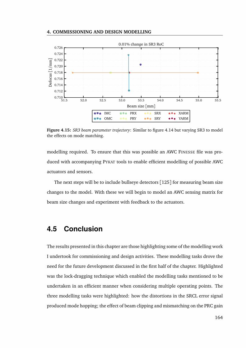
4. COMMISSIONING AND DESIGN MODELLING
51.5 52.0 52.5 53.0 53.5 54.0 54.5 55.0 55.5
Beam size [mm]
0.710
0.712
0.714
0.716
0.718
0.720
0.722
0.724
0.726D
efoc
us[1/m
m]
0.01% change in SR3 RoC
IMCOMC
PRXPRY
SRXSRY
XARMYARM
Figure 4.15: SR3 beam parameter trajectory: Similar to figure 4.14 but varying SR3 to modelthe effects on mode matching.
modelling required. To ensure that this was possible an AWC FINESSE file was pro-
duced with accompanying PYKAT tools to enable efficient modelling of possible AWC
actuators and sensors.
The next steps will be to include bullseye detectors [125] for measuring beam size
changes to the model. With these we will begin to model an AWC sensing matrix for
beam size changes and experiment with feedback to the actuators.
4.5 Conclusion
The results presented in this chapter are those highlighting some of the modelling work
I undertook for commissioning and design activities. These modelling tasks drove the
need for the future development discussed in the first half of the chapter. Highlighted
was the lock-dragging technique which enabled the modelling tasks mentioned to be
undertaken in an efficient manner when considering multiple operating points. The
three modelling tasks were highlighted: how the distortions in the SRCL error signal
produced mode hopping; the effect of beam clipping and mismatching on the PRC gain
164

at LLO; and the active wavefront control project. The former two were completed and
reported in technical notes as these were requested by commissioners to provide some
insight to the particular problems. The AWC project however is still ongoing and the
work reported here represents the initial efforts in this direction.
165

4. COMMISSIONING AND DESIGN MODELLING
166

Chapter 5
Invariance of waveguide grating
mirrors to transverse displacement
phase shifts
The paper Invariance of waveguide grating mirrors to transverse displacement phase
shifts [129] was published on the work in this chapter and presented in [43]. The
finite-difference time-domain code used for this work was developed by myself during
my masters degree [130]. This originally attempted an initial analysis of a waveguide
but needed refinement and further analysis. All the simulations performed and the
analysis was performed by myself. The plane-wave model provided in the paper was
contributed by Daniel Freidrich and general advice was given on gratings structures
by Frank Brückner and Andreas Freise. Text and figures from the paper have been
used verbatim in this chapter. Some content and formatting has been amended to fit
better into this thesis.
The sensitivity of high precision interferometry experiments such as the prepara-
tion of entangled test masses [131], frequency stabilisation with rigid cavities [132]
167

5. WAVEGUIDE PHASE NOISE INVARIANCE
and gravitational wave detectors [133] are eventually limited by the quantum noise
of the interrogating light or the thermal noise of the optical components. The high
frequency sensitivity of gravitational wave detectors is limited by quantum shot noise
which is typically improved by increasing the laser power circulating within the in-
terferometer, as discussed in chapter 1. This increase in laser power results in more
power being absorbed by the high-reflectivity coatings and substrates, inducing sub-
stantial thermal distortions. Such distortions affect both the control and performance
of the detector [53]. A number of new techniques have been suggested to reduce
both the distortions from high power beams as well as thermal noise: the use of non-
fundamental beam shapes such as the Laguerre-Gaussian modes [134]; all-reflective
interferometer layouts using dielectric gratings [135]; and the use of waveguide grat-
ing mirrors (WGM) [136].
The test mass mirrors used in advanced LIGO have approximately 40 sub-wavelength
layers applied to them to form their high reflectivity coating. Each layer in the coating
introduces additional coating thermal noise [137, 37]. This increase in thermal noise
is due to a combination of the mechanical loss from bonding multiple layers together
and that the materials used for 1064nm coatings having larger intrinsic mechanical
losses than the substrate material (Fused silica). All-reflective grating structures [135]
offer lower thermal noise as no coating stacks would be required. The all-reflective
nature of such designs mean that alternative materials could be explored which pro-
vide preferable thermal noise levels. However, it was found that gratings can couple
relative transverse displacements between itself and the incident beam into the phase
of the non-zero diffracted orders [138, 139]. This coupling placed stringent require-
ments on the alignment and stability of gratings and the incident laser beams so as
not to induce additional phase noise when used in gravitational wave detectors [140].
Another option being discussed at the time was the use of waveguide grating mir-
rors to replace more traditional coating stacks. Waveguide grating mirrors would re-
168

place the high reflectivity mirror coating stacks used on fused silica substrates with just
two separate layers, reducing their thickness by a factor of 10 to 100. This promised to
reduce the Brownian coating thermal noise [133, 141]. However, as WGMs also rely
on diffraction into the first order the concern was at the time that the susceptibility to
the transverse displacement coupling could negate these benefits.
This work was undertaken to demonstrate that waveguide grating mirrors are not
susceptible to this transverse phase coupling. Both a theoretical and numerical argu-
ment was published. In this chapter I first provide a simplified plane wave picture of
why no transverse to longitudinal coupling should exist in section 5.1. This is then
verified by using a rigorous Maxwell equations solver using finite Gaussian beams in
section 5.2. The finite-difference time-domain (FDTD) solver of Maxwell’s equations
was programmed by myself to obtain a clearer understanding of the accuracy and
limitations of such a model. This code was also used for the modelling of transverse
displacement phase coupling for standard grating structures as part of an experimental
project. This work was reported on and published in both [139] and [142].
5.1 Waveguide grating mirrors
Waveguide grating mirrors in their most simplistic form consist of two layers: (i) a
waveguide layer applied to some substrate material; and (ii) a grating layer which
couples the incident laser light into the latter [136]. The grating layer can be etched
into the waveguide layer thus creating a lower loss single layer compared to multiple
stacks of dielectric coatings [141]. In this case both the waveguide and grating layers
are then made from the same high refractive index nh material, the substrate material
then has a refractive index nl . The materials used for 1064nm light are fused silica
for the substrate and Tantalum pentoxide for the high refractive index material. A ray
picture of an incident plane wave interacting with the WGM is shown in figure 5.1.
169

5. WAVEGUIDE PHASE NOISE INVARIANCE
vacuum
Figure 5.1: The ray picture [129]: The incident beam (black) is coupled into the waveguidelayer by the grating into m = ±1. Orders ±1T propagate along the waveguide coupling backinto the vacuum (blue) to interfere with the initially reflected light, 0R, picking up∆Φm phaseterms with each interaction with the grating. Further coupling into the vacuum is also possible(magenta) which involved further ∆Φm terms. The ∗ superscript refers to the number ofdiffractions beam has undergone. R=Reflection from grating, T =Transmission from grating,first number is order of diffraction m.
For given materials and laser light wavelength, the grating period d must be chosen to
form a Littrow configuration, where a normally incident beam is diffracted on trans-
mission into the 1st orders within the waveguide layer. The angle at which these modes
are diffracted must allow total-internal-reflection (TIR) at the waveguide-substrate
boundary to occur (This requires nl < nh). These reflected modes are then diffracted
once again by the grating layer. TIR at the substrate boundary along with the grating
create a waveguide in which the ±1st orders propagate along. These undergo diffrac-
tion at the grating multiple times, each time coupling out into the vacuum where it
interferes with the reflected laser light. The remaining grating parameters, namely
the thickness of the waveguide layer s, fill-factor f and groove depth g, along with
the geometrical grating parameters must be carefully chosen to produce a theoretical
100% reflectivity [136, 141] which occurs in the diffracted and specularly reflected
light undergo perfect constructive interference.
A transverse displacement δx of a grating structure relative to the incident beam
induces a phase shift of [140]:
∆Φm = 2πmδx/d. (5.1)
170

This phase shift is relative to the phase already accrued by a non-displaced beam
diffracted into the mth order, ∆Φm = 0. For WGMs to experience no transverse to
longitudinal phase coupling it must be ensured that any of the rays interfering with
the specularly reflected field do not have any phase terms dependent on δx . From
figure 5.1 each time a ray is diffracted it picks up an additional ∆Φm term. Here an ∗is added as a superscript each time this has happened. Examining figure 5.1, the ray
−1T ∗∗ diffracted into the vacuum has collected two∆Φm terms. The total accumulated
phase in the field is then:
Φ−1T ∗∗ = Φo(s, d, g, f , nl , nh) +∆Φ+1 +∆Φ−1, (5.2)
where Φo is a collection of the additional phase terms accumulated that depends on
the WGM parameters, but not δx . Φo is tuned by adjusting each parameter to produce
100% reflectivity as required for a WGM to function.
From Eq.(5.1) it can be seen the∆Φ−1 and∆Φ+1 terms cancel. A similar argument
is valid for all other rays that couple out to interfere with the directly reflected field,
such as +1T ∗∗∗. Thus, following this simplified picture any of the phase noise effects
outlined in [140] for gratings should not apply to WGMs under normal incidence.
5.2 Numerical experiment
In order to provide a rigorous and more physically correct model of a finite beam
reflected from a WGM, a numerical finite-difference time-domain (FDTD) based al-
gorithm was used. This provided the ability to model a variety of grating structures
as well as arbitrary and finite incident electromagnetic field distributions. The sim-
ulation tool was coded myself in the Java language. It is open sourced and can be
found at http://kvasir.sr.bham.ac.uk/redmine/projects/fdtd), the code
171

5. WAVEGUIDE PHASE NOISE INVARIANCE
itself is based on the work of Taflove who pioneered much of the FDTD field [143]. As
only a displacement of the WGM in one direction orthogonal to a normally incident
Hermite-Gaussian beam was required, A 2D FDTD simulation also sufficed. To perform
the simulation two features were also required for the simulation [143]: Total-Field
Scattered-Field (TFSF) for separating the incident and reflected beam from the WGM
and complex perfectly matched layers (CPML) to reduce reflections from the simulation
boundaries.
The aim of the simulation was to measure the wavefront of a Hermite-Gaussian
beam reflected from a WGM whilst displacing it from δx = 0→ d. Along the wave-
front the phase can then be deduced and plotted against δx to view any apparent
phase shifts. The simulation setup is depicted in Fig.5.2, where a Hermite-Gaussian
TEM00 is injected in the x direction along the TFSF boundary and the electric field of
the reflected beam is measured along the measurement line 15µm away to avoid near-
field variations. The Courrant stability factor [143] for the simulation was chosen as
S = c∆t/∆x = 1/p
2; where ∆t is the simulation time-step and ∆x = ∆y = 25nm
are the size of the 2D discretisation of the simulation space with dimensions L y =
250∆y and Lx = 4000∆x . The injected beam had a wavelength λ = 1064nm and
was positioned such that the waist was at the WGM with size w0 = 800∆x = 20µm.
The WGM parameters chosen were d = 28∆x = 700nm, g = 14∆x = 350nm, f = 0.5
and s = 5∆x = 125nm which provided a reflectivity of 99.8% for the incident beam (in
agreement with [136]). The indices of refraction used were fused silica for nl = 1.45
and Ta2O5 for nh = 2.084 which are the typical materials used for 1064nm optics.
The phase shift for m= ±1 is periodic with displacements of the grating period d =
28∆x as can be seen from Eq.(5.1). Thus, for this effect to be visible the simulation
was run multiple times for the offsets δx = p∆x with p = 0, 1,2, ..., 28; 28 samples
were used as this ensured integer steps in offset as FDTD is based on discretised space.
To compare the phase of the beam for each offset the steady state of the reflected field
172

Figure 5.2: Simulation setup [129]: Schematic layout of 2D FDTD simulation for testing WGMshift invariance. Gaussian beam injected along TFSF boundary onto WGM (Red). The reflectedbeam (Green) then propagates to the measurement line where the phase is measured. TheCPML absorbs outgoing waves to reduce reflections from boundaries.
must be found. Approximately 3000 time steps were required for the reflected beam
to reach an approximate steady-state in each simulation. Once reached, 1024 time
samples of the electric field,Ep(x , t), at each point along the measurement line were
taken to extract the phase from. The generalised Goertzel algorithm (based on Fast
Fourier Transforms (FFT)) [144] was used to extract both the amplitude Ap(x) and
phase φp(x) of the reflected beam along the measurement line for the incident laser
frequency f0 = c/1064nm. φp(x)was obtained for each offset δx = p∆x of the WGM
with the change in phase with displacement defined as ∆φp(x) = φp(x)−φ0(x).
The simulation showed that displacement phase shift for WGMs are at least 105
smaller than for an equivalent grating setup, see figure 5.3. The central plot shows
the phase change as a function of the displacement along the beam profile; the satel-
lite plots provide the scale for the central plot. The top plot shows ∆φ14 increasing
slightly towards the edge of the beam, this is expected to occur when Ap(x) → 0,
which degrades any accurate calculation of the phase as the signal-to-numerical noise
ratio decreases. At the beam’s peak intensity the phase change with WGM offset is
∆φp(x = 0)≈ 20µrad, this also shows no real dependence on δx . This phase change
is five orders of magnitude smaller than what Eq.(5.1) states for displaced grating
173
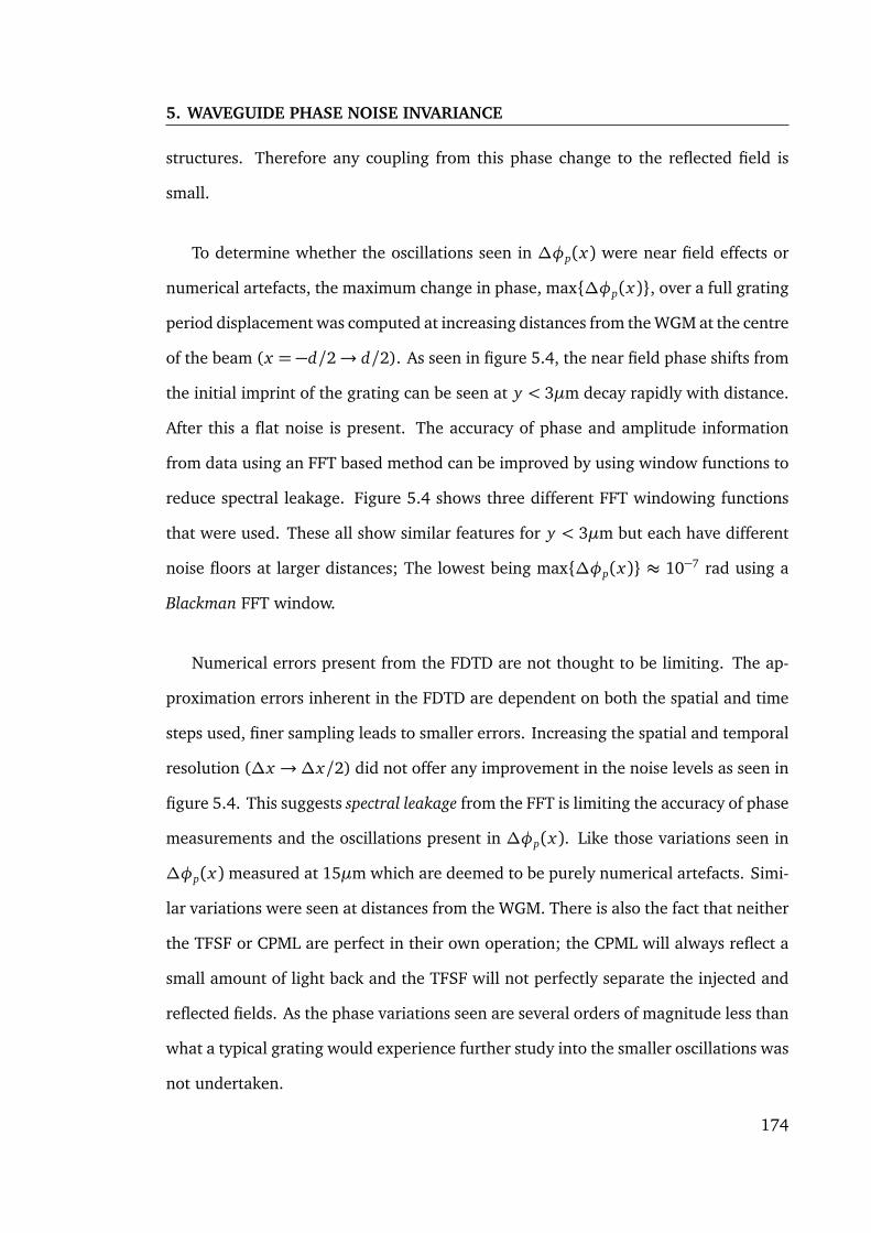
5. WAVEGUIDE PHASE NOISE INVARIANCE
structures. Therefore any coupling from this phase change to the reflected field is
small.
To determine whether the oscillations seen in ∆φp(x) were near field effects or
numerical artefacts, the maximum change in phase, max∆φp(x), over a full grating
period displacement was computed at increasing distances from the WGM at the centre
of the beam (x = −d/2→ d/2). As seen in figure 5.4, the near field phase shifts from
the initial imprint of the grating can be seen at y < 3µm decay rapidly with distance.
After this a flat noise is present. The accuracy of phase and amplitude information
from data using an FFT based method can be improved by using window functions to
reduce spectral leakage. Figure 5.4 shows three different FFT windowing functions
that were used. These all show similar features for y < 3µm but each have different
noise floors at larger distances; The lowest being max∆φp(x) ≈ 10−7 rad using a
Blackman FFT window.
Numerical errors present from the FDTD are not thought to be limiting. The ap-
proximation errors inherent in the FDTD are dependent on both the spatial and time
steps used, finer sampling leads to smaller errors. Increasing the spatial and temporal
resolution (∆x →∆x/2) did not offer any improvement in the noise levels as seen in
figure 5.4. This suggests spectral leakage from the FFT is limiting the accuracy of phase
measurements and the oscillations present in ∆φp(x). Like those variations seen in
∆φp(x)measured at 15µm which are deemed to be purely numerical artefacts. Simi-
lar variations were seen at distances from the WGM. There is also the fact that neither
the TFSF or CPML are perfect in their own operation; the CPML will always reflect a
small amount of light back and the TFSF will not perfectly separate the injected and
reflected fields. As the phase variations seen are several orders of magnitude less than
what a typical grating would experience further study into the smaller oscillations was
not undertaken.
174

δ x
[n
m]
∆φp(x) against WGM displacement, δ x
−60 −40 −20 0 20 40 600
350
700−60 −40 −20 0 20 40 60
−2
0
2φ
14(x
) [
mra
d] Change in phase ∆φ
14(x) δ x = 350nm
0
350
700
02040∆φ
p(x=0) [µrad]
−60 −40 −20 0 20 40 600
0.5
1
x [µm]
|A0(x
)|2
Figure 5.3: Waveguide displacement phase shifts [129]: Central plot shows phase change inthe reflected beams wavefront ∆φp(x) against WGM displacement, δx . Top plot shows crosssection of phase at δx = 350nm where the phase change is maximum. The right plot showsthe variation in the phase of at x = 0 against δx . Bottom plot shows the intensity of thereflected beam along x .
0 5 10 15 20 25 30 35 40 4510
10
105
100
Distance from WGM surface [µm]
max
p
[rad]
Rectangular Hanning Blackman Rectangular x/2
Figure 5.4: Numerical noise floor [129]: Maximum change in phase at beam peak intensity asthe WGM is displaced from δx = 0→ d with increasing distance from the WGM surface anddifferent FFT windowing functions. Large near field phase shifts are seen close to the WGMand then a flat noise. Increasing the spatial and temporal resolution of FDTD∆x →∆x/2 didnot appear to offer reductions in numerical noise caused by FDTD.
5.3 Conclusion
Before this work no experimental or theoretical work had been published on the
waveguide grating mirrors susceptibility to transverse displacement phase noise. This
work used a rigorous FDTD simulation to analyse displacement induced phase shifts
175

5. WAVEGUIDE PHASE NOISE INVARIANCE
in a reflected Gaussian beam from a waveguide grating mirror. It was found that this
coupling did not affect the waveguide grating mirrors for a perfectly normal incident
beam, within the precision limit of ≈ 10−7 rad set by numerical errors. This limit is
seven orders of magnitude lower than the phase noise estimated for previously pro-
posed layouts with diffraction gratings, which raised concerns regarding the stability
and alignment [140] of such grating based configurations. Therefore, the absence of
this phase shift for WGMs removes one of the concerns for their usage in future high-
precision interferometry experiments, motivating further research into such coatings.
Since the publication of this work, research elsewhere has continued on the devel-
opment of WGMs for third generation detectors [145, 146]. Experimental efforts at
the Glasgow 10m prototype have also confirmed our results showing no significant
transverse to longitudinal couplings to one part in seventeen-thousand [147].
176

Chapter 6
Summary and conclusions
In this thesis I have described the development of new modelling techniques and their
application in the study of advanced gravitational wave detectors, in particular for
commissioning of Advanced LIGO and the design of future upgrades to LIGO and new
detectors such as the Einstein Telescope. It is crucial in the development of numerical
models that strong efforts are made to verify them by comparing its predictions with
current experimental results. The simulation programme FINESSE, which is at the core
of my research work, has been successfully used and verified during the commissioning
of gravitational wave detectors by myself and others. I have then used this well tested
and vetted code base to develop more powerful modelling techniques and explore new
interferometer ideas.
FINESSE is a popular simulation tool capable of modelling steady-state interfer-
ometers. It has seen extensive use in previous generations of detectors, table top
experiments and prototypes for design and commissioning purposes. As a result of
my work, FINESSE’s feature set was significantly expanded to accommodate the mod-
elling needs of future detectors. FINESSE was also open sourced and actively main-
tained across Windows, OSX and Linux during my PhD, whilst responding to queries
and bug reports from users across the gravitational wave community and beyond.
177

6. SUMMARY AND CONCLUSIONS
Due to advanced detectors using a combination of high laser powers and suspended
optics the pressure exerted by the lasers becomes significant within the interferome-
ter. In such cases the interferometer is transformed into an optomechanical system,
where its optical and mechanical response is greatly altered by the appearance of
optical springs. To enable such effects to be studied I have implemented significant
changes to internals of FINESSE. It is now able to model steady-state optomechanical
coupling effects—including longitudinal, rotational and higher order surface motions
of suspended optics—that are driven by radiation pressure exerted by higher order
modes of the lasers light.
In current and future detectors, low loss and high quality factor materials are used
for constructing the test masses. The vibrational modes of the test masses coupled with
high laser power can result in parametric instabilities; vibrational modes pumped by
the optical field that have a growing amplitude. These instabilities are expected to
be problematic by causing lock losses and have already been experimentally seen in
aLIGO. Here, I develop an idea for an optical configuration that offers a broadband
suppression of parametric instabilities. Thus far only mechanical suppression of para-
metric instabilities acting locally at each mirror have been considered. Although not
applicable to LIGO as it is, the scheme proposed could be incorporated into future
designs. This work is currently being prepared for publication: Daniel Brown et al.
Optical suppression of parametric instabilities with extraction cavities. 2015. In prepa-
ration.
During my PhD I also actively participated in the commissioning modelling for
aLIGO, the work accomplished is reported in chapter 4. As part of a team of simulators
we actively maintained an up to date FINESSE script of the LHO and LLO detectors.
This was used to respond to requests from commissioners to unexpected behaviours in
the interferometers. In this chapter I have highlighted two problems that I contributed
towards: the study of error signal distortions that were giving rise to control issues
178

at LHO; and the study of how beam clipping resulted in unexpectedly low power
recycling cavity gains. In these cases the work was reported by the modelling team
in several technical notes published to the LIGO document control center. A list of
technical notes can be seen in the ‘List of publications’ section in the back matter of
this thesis.
Throughout my development of FINESSE I have tried to ensure that it remained
as fast as possible. Faster simulations allow simulators to respond quicker to com-
missioning request and generally be more efficient at exploring problems involving
high-dimensional parameter spaces. One aspect where significant improvements were
made was in the use of reduced order quadrature, as outline in chapter 2. Collaborat-
ing with Rory Smith, we created a vastly improved numerical integration algorithm
was developed for modelling optical mode scattering. Computational performance of
the order of a thousands times were seen, greatly expanding the modelling capabili-
ties of FINESSE. This work has been submitted for publication in: Daniel Brown, Rory
Smith, and Andreas Freise. Fast simulation of gaussian-mode scattering for precision in-
terferometry. Journal of Optics, Sept 2015. Submitted on 2nd of September, awaiting
feedback.
Also reported here was is the study I undertook in regards to the use of waveguide
grating mirrors and their suitability for use in gravitational wave detectors. These mir-
ror use a grating and waveguide structure to produce a near-perfectly reflective mirror
but with a substantial reduction in coating thermal noise compared to dielectric coat-
ing stacks. However, there were concerns that the grating structures could introduce
a new noise coupling from lateral displacements to the phase of the diffracted orders.
Using a numerical finite-difference time-domain code for solving Maxwell’s equations
I demonstrated this noise coupling did not affect waveguide grating mirrors, down
to levels of numerical and post-processing errors. Thus removing a potential concern
for their use in future detectors. This work was published in: Daniel Brown, Daniel
179

6. SUMMARY AND CONCLUSIONS
Friedrich, Frank Brückner, Ludovico Carbone, Roman Schnabel, and Andreas Freise. In-
variance of waveguide grating mirrors to lateral displacement phase shifts. Opt. Lett.,
38(11):1844–1846, Jun 2013.
6.1 Outlook
Looking forward, the modelling of advanced detectors is currently reaching an inter-
esting era. Both of the LIGO detectors have successfully completed their initial com-
missioning and have now started their first scientific data taking run. Already para-
metric instabilities have been detected at ≈ 30 W of input power. As this is gradually
increased in future commissioning efforts parametric instabilities and other radiation
pressure will become even more apparent. The FINESSE modelling team is now poised
and ready with the necessary tools and experience to play their part in investigating
this new and unexplored high power regime.
Also developed and implemented in FINESSE during my PhD were substantial ad-
ditions to the quantum noise calculations (See appendix D). It is only recently that
these features have started to be used in designing new interferometric devices, such
as ET and the Glasgow speed meter prototype. These features were also being put to
use in studying how mode-matching affects the quantum noise limited sensitivity as
part of the active wavefront control project. This project started near the end of my
PhD and will be continued by others; the modelling effort started here will enable fu-
ture research into possible control and sensing schemes for better mode-matching. In
the future there also lies interesting modelling possibilities for studying higher order
modes in quantum-limited systems, for example, the effects of spatial distortions on
balanced homodyne readout, the limits to the effectiveness of squeezed light injection
due to spatial distortions and more realistic models of the many new ideas to over-
come quantum noise, such as speed meters or active filters. Experimental efforts on
180

both table-top and prototype scales have now started and will provide exciting results
which can be used to continue the process of the testing and advancing our numerical
models.
181

6. SUMMARY AND CONCLUSIONS
182

Appendix A
Interferometer simulation tool:
Finesse
On their own each of the optical features described in the chapter 1 are not especially
complicated. However, great complexity arises when combining all these features to-
gether. Calculating the fields by-hand is a time consuming process for systems more
complicated than a single cavity: FINESSE was created as a solution to this problem.
In 2012 when I took over the development of FINESSE it was already a popular tool
within the community. However, it was lacking in several key physical features for
modelling advanced detectors: radiation pressure effects, thermal distortions and scat-
tering and quantum noise calculations. These features were desired by the community
and actively requested over the years but had unfortunately lacked the developer to
accomplish this.
The improvements and additional features added to FINESSE by myself are per-
haps the most significant output of my PhD. This is a tool that will be used long after
the completion of my PhD for the learning, designing and commissioning of future
gravitational wave detectors.
A great deal of time was spent programming and testing the new features. This
183

A. INTERFEROMETER SIMULATION TOOL: FINESSE
work has enabled both myself and others to accomplish new research. Some examples
of where my work has enabled others to study new problems with FINESSE is in the
KAGRA OMC design [148], studying thermal correction in GEO600 [149], studying
the use of Laguerre-Gaussian beam shapes for thermal noise reduction [150, 151] and
thermal distortion effects in aLIGO [53]. These all made use of the new scattering
features implemented. The use of quantum noise and radiation pressure effects are
currently being used in design work for ET and the speed meter prototype [152]. It
is also actively used for aLIGO commissioning simulations and future aLIGO design
upgrades, as highlighted later in this chapter, and for studying higher order mode
radiation pressure effects, as discussed in chapter 3.
This section will provide an outline of the improvements made over my PhD. Spe-
cific aspects of the coding won’t be discussed here; the source code is freely available
for those wishing to browse the ≈ 76500 lines of code at https://gitmaster.
atlas.aei.uni-hannover.de/finesse/finesse. The FINESSE manual contains
more information regarding the technical aspects of features and how to use them [26].
FINESSE is a terminal based, open source (GPL 2) cross platform binary called kat.
It is written in C and was mostly developed on Unix based systems. Windows support
was achieved using both the Cygwin and MinGW projects. It uses a simplified scripting
language to produce what is referred to as a FINESSE file or a FINESSE script. These
scripts are then fed into the kat binary from a terminal and a text based output file
is generated on completion along with a Gnuplot or Python interactive plot of the
outputted results.
The scripting language allows the user to define arbitrary interferometer layouts
consisting of mirrors, beamsplitters, isolators, modulators, lenses and diffraction grat-
ings. They are then connected together in a nodal network by defining the space be-
tween each component. It operates in either a plane-wave or Hermite-Gaussian beam
mode, thus the geometry of mirrors and beamsplitters is also definable.
184

Parse kat fileAllocate memoryfor component
structures
Create nodalnetwork,
count opticalfrequencies,
process inputs
Initialisesettings
Count elements andlayout interferometer
matrices
Allocate matrixmemory
Link matrix memory tocomponent structures
Compute cavityeigenmodes,
do beam trace
Calculatescatteringmatrices
Beamparameters not set
or changed?
Yes
Fill/updateinteferometer
matrix elements
Update variablesfor currentdatapoint
No
Fill carrierRHS, solve
carriermatrix
Locks enabled?
Apply controlfeedback
YesError signals
zeroed?
No
YesNo
Fill signalRHS, solve
signalmatrix
Anymore data
points?
Yes
Save outputfiles
No
Free memory
Using signalfrequencies?
Compute classical and quantumdetector outputs
Yes
No
Figure A.1: Flow of FINESSE: A general overview of the operation when running a givenFINESSE file using higher order optical modes.
Once the layout is defined the user can then add a number of different detectors
to extract information from the simulation. These range from realistic demodulated
multi-quadrant photodiodes and CCD cameras to unphysical detectors that directly
output the amplitude and phase of a particular HOM at any location.
With the components and detectors set up the file must then state what type of
simulation to run. A minimum and maximum range of one or more of interferometer’s
parameters are then specified to be simulated; then for each of these steps the output
of all the detectors specified will be written to an output text file. An overview of the
process of running a script is shown in the flow diagram in figure A.1.
185

A. INTERFEROMETER SIMULATION TOOL: FINESSE
Core matrix solver
One of the largest changes I made to FINESSE was in the way that it handled the in-
terferometer matrix. Originally FINESSE was designed for memory efficiency due to
computers having limited amounts of RAM; as large interferometer files can easily
end up consuming multiple gigabytes when using a high Omax with multiple optical
frequencies. The shape of the interferometer matrix is identical for each optical fre-
quency, e.g. Eq.(1.59), thus a single matrix propagating a single optical frequency
could be created. To solve for the optical fields this matrix was iterated over for each
frequency and its elements updated with the appropriate optical frequency.
Although this was ideal for memory usage, it did not allow for either radiation
pressure effects or sidebands-of-sidebands [153] to be modelled: a feature of linking
sequential optical modulators. This is because both effects require computing the cross
coupling between optical fields, something that cannot be achieved if they are solved
individually.
The entire matrix construction and filling routines were rewritten for this, the pro-
cess of which uses the sub-matrix block methods laid out in section 1.3.3. In total
two matrices are created in FINESSE now: one for the main carrier and the RF side-
bands, the carrier matrix; and another for the signal sidebands pairs around each of
the carriers and RF sidebands, the signal matrix. The carrier matrix represents the
steady-state of the main optical fields. The signal matrix then represents small and
linear perturbations of each of the carriers at a particular frequency Ω, such as those
induced by a gravitational wave or noise source. This signal matrix is important for
implementing radiation pressure effects and quantum noise calculations.
It was important to ensure these changes still produced the same results for existing
files. To do this a Python test server was setup which checked each Git commit pushed
to the main FINESSE repository. This takes each commit and builds the corresponding
kat binary. A collection of several hundred scripts is then ran and the outputs com-
186

pared to reference outputs to check whether a commit has altered or broken anything.
A web interface allows easy viewing of which files were altered and can display the
history of which commits produces different values. Overall the differences in all the
script outputs tested were better than 10−10 in relative error before and after the core
matrix solving changes.
Maps and scattering
Before I began developing FINESSE and initial implementation of higher order mode
scattering as described in section 1.3.3.2 was included. As noted in the aforemen-
tioned section the handling of maps must be done carefully. There were several issues
in the way that FINESSE use to handle multiple maps and combining several scattering
matrices; these issues were all fixed to operate as described in section 1.3.3.2.
Another technical issue was in efficiently performing the numerical integration for
the scattering matrices. The original scattering calculations would take on the order of
several hours to days depending on the simulation performed. Chapter 2 outlines the
final solution to this issue using reduced order quadrature, which effectively removes
the computational cost of evaluating the scattering matrices.
Radiation pressure
With the successful implementation of the new signal matrix construction a linearised
model of radiation pressure effects were included in FINESSE. The model used as-
sumes that the actual displacements induced by radiation pressure effects is always
λ. The implementation of this requires that the upper and lower audio sidebands
can be coupled at a suspended mirror, hence why the new matrix construction was re-
quired. More details on the radiation pressure effects implemented are left to discuss
in chapter 3.
187

A. INTERFEROMETER SIMULATION TOOL: FINESSE
Quantum noise
Originally FINESSE could only compute the shot noise measured at a demodulated
photodiode due to vacuum noise. For future detectors it was required to extend this
to include squeezed states of light and how radiation pressure effects due to increased
circulating optical field powers altered the noise couplings.
The quantum noise computations I added to FINESSE allowed for computing the
full quantum noise effects with radiation pressure effects for general demodulated
photodiodes and balanced homodyne detectors. Appendix D provides an overview of
how these calculations work. These quantum noise calculations features are now be-
ing used for ET and the Glasgow speed meter modelling and for the AWC modelling.
Thus far commissioning tasks have not been centred around problems regarding quan-
tum noise. But this will eventually change going forward when the squeezer and filter
cavities are designed and installed in planned LIGO upgrades.
188
Appendix B
Pykat: Python wrapper for Finesse
For more advanced FINESSE modelling, along with the core C engine, a Matlab based
toolbox SIMTOOLS [154] was available. The core engine of FINESSE is run using a
single script file but for more complex modelling tasks that involve iterating over a
parameter space, optimising results, or automation of tasks a higher level interface is
required. SIMTOOLS was used extensively for all of the commissioning modelling and
others that were undertaken in C. Bond’s thesis [53].
PYKAT originally started as an experiment for visualising FINESSE scripts: variables
used, optical layouts, beam parameters, etc., for easier debugging of long files as
shown in appendix E. However, this was supplanted by providing a more feature rich
replacement of SIMTOOLS. All the modelling described in this thesis was undertaken
using PYKAT (bar some of the commissioning modelling reported).
Python was chosen as it offers all the programmatic features that were required
whilst being both free and open sourced. Other simulation tools within the gravita-
tional wave community rely on Matlab and expensive toolboxes, meaning licenses are
required just to experiment with them. A particular nuisance is the lack of free access
to parallel programming features in Matlab without the designated toolboxes. With
ever more complex models being made access to multiple cores was crucial for com-
189

B. PYKAT: PYTHON WRAPPER FOR FINESSE
missioning and design activities and another driving reason the move to Python was
made.
PYKAT was designed with a few key ideas in mind:
- Open source and cross platform support
- Object-orientated design for constructing and manipulating FINESSE files
- Lightweight and succinct interface
- A central repository for helpful tools and functions for FINESSE modelling
- A rolling support of FINESSE features as they are required. Not all features need
to have a PYKAT equivalent to use them immediately, a user can always revert
back to adding in specific commands by hand.
It is available for both Python versions 2.6+ and 3+ and can be downloaded from [67].
Today PYKAT has displaced SIMTOOLS for advanced modelling tasks with many of its
scientifically useful features now ported to Python.
The core part of PYKAT is the pykat.finesse.kat class. This will read and parse
the commands in a FINESSE file into itself as properties of the class. For example, here
the commands to create a plane-wave Fabry-Perot cavity are loaded into PYKAT:
Code B.1 PYKAT example
import pykat
kat = pykat.finesse.kat() # Create the main Finesse object
kat.parseCommands("""
l l1 1 0 n0 # Input laser
m m1 0.9 0.1 0 n0 n1 # Input mirror
s s1 1 n1 n3
m m2 0.99 0.01 0 n2 n3 # End mirror
190

pd circ n1 # Circulating power
pd refl n0 # Reflected power
pd trans n3 # Transmitted power
xaxis m1 phi lin 0 180 180 # Scan m1’s tuning over half a wavelength
""")
output1 = kat.run() # Run the first simulation ...
kat.l1.P = 2 # Access the laser like an object
# by changing the power ...
output2 = kat.run() # Run again ...
# Finally just output the photodiode powers
print(output1["circ"], output1["refl"], output1["trans"])
print(output2["circ"], output2["refl"], output2["trans"])
When run, the kat object reproduces a file that is passed to the FINESSE executable.
Parameters of any object can be accessed in a typical object orientated manner, such
as the input laser power shown here. Once finished running the data is parsed and
outputted into the output objects output1 and output2. From these the calculated
values can be accessed, manipulated or saved to file.
Another aim for having this object orientated representation of the script files is
to create functions that operate on a FINESSE script file. For example, a function was
created that removed subsections of the interferometer when note needed, such as
the IMC. In such cases additional mode-matching must be done to ensure the file
still works, again an aspect that is automated. Other examples are functions that
given some kat object of an aLIGO interferometer will proceed to compute a length
or alignment sensing matrix. This involves running multiple simulations and collecting
results, something which is run multiple times for different interferometer parameters.
Lastly having this object representation eases the parallelisation of running multiple
FINESSE simulations at once. Built in is support for starting and collecting the results
from running many simulations using the IPython cluster software. Such a feature was
crucial for running parametric instability models as discussed in chapter 3.
191

B. PYKAT: PYTHON WRAPPER FOR FINESSE
PYKAT also enables other software to interface with FINESSE scripts in new ways.
A great example of this is OPTIVIS (https://github.com/SeanDS/optivis), a
graphical interface for creating interferometer layouts using SVG graphics written by
Sean Leavey. Sean and myself worked together to enhance this further, allowing a
FINESSE file to be read, displayed and then altered through the graphical interface.
Outlook
A more ergonomic and powerful wrapper was required for FINESSE to enable more
efficient modelling of complicated problems. PYKAT was successful in providing the
required features that users demanded of it and is now used exclusively by those doing
advanced modelling with FINESSE.
At the end of my PhD PYKAT would be classed as a beta version. Overall it is a
stable package that greatly enhances the modelling capabilities of FINESSE. A few
bugs still remain as well as missing some of the advanced FINESSE features have not
year been wrapped in PYKAT code: such as, maps, FINESSE functions, and various
beam tracing outputs. However, in time these will be added as they are required.
All the code is open sourced and accessible from https://gitmaster.atlas.aei.
uni-hannover.de/pykat or via PYPI package manager.
192

Appendix C
Rotational radiation pressure
This appendix outlines the analytic math to compute the scattering matrices for rota-
tional modes of a mirror. These are required for computing optomechanical coupling
as outline in chapter 3: thus, this appendix should be read in context with that chapter.
Yaw and pitch motions
The next order of motion possible after longitudinal motions of rigid object are rota-
tions. When considering any tilting motion the functional form of the surface motion
is zs(x , y) = x or zs(x , y) = y , for yaw or pitch respectively: thus the motion has
units of radians. To analytically solve this we will make use of the orthogonality of the
Hermite-Gaussian polynomials again, consider the scattering from yaw motion which
is represented by K x :
K xnmn′m′ =
∫∫ ∞
−∞unm(x , y) x u∗n′m′(x , y)dx dy, (C.1)
=
∫ ∞
−∞un(x) x u∗n′(x)d x
∫ ∞
−∞um(y)u
∗m′(y)dy, (C.2)
= δmm′
∫ ∞
−∞un(x) x u∗n′(x)dx = δmm′K
xnn′ . (C.3)
193

C. ROTATIONAL RADIATION PRESSURE
Using the 1D Hermite-Gaussian beam of order n:
un(x) =
2π
14 ei (n+1/2)Ψ(z)
p2nn!w(z)
Hn
p2x
w(z)
e−
x2
w2(z) e−i kx2
2Rc(z) (C.4)
= CnHn
p2x
w(z)
e−
x2
w2(z) e−i kx2
2Rc(z) (C.5)
and the substitution x =p
2x/w(z):
K xnn′ = CnC∗n′
w2x(z)
2
∫ ∞
−∞Hn( x) x H∗n′( x)e
− x2d x . (C.6)
To make use of the polynomial orthogonality we can substitute in another polynomial
2 x = H1( x):
K xnn′ = CnC∗n′
w2x(z)
4
∫ ∞
−∞Hn( x)H1( x)H
∗n′( x)e
− x2d x (C.7)
Using the identity for Hermite products:
Hn(x)Hm(x) =min(n,m)∑
r=0
2r r!
nr
mr
Hn+m−2r(x), (C.8)
we find:
K xnn′ = CnC∗n′
w2x(z)
4
min(n,n′)∑r=0
2r r!
nr
n′
r
∫ ∞
−∞H1( x)Hn+n′−2r(x)e
− x2d x . (C.9)
The value of this integral can be found using the orthogonality of the Hermite-Gaussian
polynomials,∫∞−∞Hn(x)Hm(x)e−x2
dx =pπ2nn!δnm. Applying this result we are left
with:
K xnn′ = CnC∗n′
pπw2
x(z)min(n,n′)∑
r=0
2r−1r!
nr
n′
r
δ1,n+n′−2r . (C.10)
The only non-zero terms of the summation are when r = (n+n′−1)/2. The conditions
on r are that it is a positive integer, r must be in the range 0 ≤ r ≤ min(n, n′), and
194

n+ n′ must be odd. These are met only when |n− n′| = 1. Thus an incoming mode
only couples to n = n′ ± 1 for small yaw motions. The only non-zero elements in the
scattering matrix are then:
K x(n′+1)n′ =
pn′ + 12
wx(z)eiΨx (z) K x
n′(n′+1) = K x∗(n′+1)n′ (C.11)
K x(n′−1)n′ =
pn′
4wx(z)e
−iΨx (z) K xn′(n′−1) = K x∗
(n′−1)n′ (C.12)
This simple result is ideal as it removes a computationally expensive integration re-
quired to compute the scattering terms. This is particularly useful in cases where one
is interested modelling how changes in beam shapes might affect radiation pressure
coupling.
It should be noted that this scattering matrix differs from those examined in sec-
tion 1.3.3.2, as the elements are not necessarily in the range 0 ≤ |K xnn′ | ≤ 1. This is
due to the fact a linearised version of the equations are used and the magnitude of
the motion As has been factored out. Thus, it must be kept in mind that |As| 1. No
energy conservation is broken as only very small amounts of power are scattered into
these sidebands. It should also be noted that the above result is exactly the same for
the pitch motion, only a change in superscript from x → y and subscript n → m is
required.
Finally, the coupling from yaw motions, As → θx , and pitch, As → θy , to the scat-
tered sideband amplitude is:
a±s, jnm = i rk∑n′,m′
ac, jn′m′θ±x (K
x K o)nmn′m′ + θ±y (K
y K o)nmn′m′
(C.13)
where as the notation as previously used for longitudinal case means θ+x/y ≡ θx/y and
θ−x/y ≡ θ ∗x/y .
195
C. ROTATIONAL RADIATION PRESSURE
Optical field to rotation
An optical field can also apply a torque if the beam is off-centred or of some distorted
shape. For this we must determine the centre-of-intensity, analogous to a center-of-
mass computation. This can be computed by the integration:
∆x =
∫∫ ∞
−∞
x I(x , y, t)P
d xd y (C.14)
where P is the total power of the beam and I(x , y) is the intensity at a given point.
Computing ∆y is merely a task of swapping x for y in the integrand. Using equation
3.34 we find:
∆x =1P
∫∫ ∞
−∞x E(x , y, t)E∗(x , y, t)d xd y, (C.15)
=∆xDC +∆xs(Ω)e−iΩt +∆xs(−Ω)e−iΩt +O(a2
s ) +O(|ω Ω|). (C.16)
Whereby expanding the E∗E product we again find multiple frequency components:
∆xDC represents DC offsets of a beam and ∆xs represents offsets that are oscillating
with frequency Ω. We have also truncated some of the terms, namely those that are
order |as|2 which are negligibly small and those with a frequency term much greater
than the motion frequency Ω. This latter truncation is possible because mechanical
susceptibility of a suspended mirror is ∝ Ω−2, thus RF frequency components con-
tribute negligible amounts to the torque applied compared. Therefore, we are con-
cerning ourselves primarily with terms that oscillate at Ω as it is assumed DC levels
will always be compensated by some active or passive control to keep the static mirror
196

rotations aligned. Expanding and collecting all Ω terms we find:
K xnmn′m′ =
∫∫ ∞
−∞unm(x , y) x u∗n′m′(x , y)dx dy, (C.17)
∆xs(Ω) =1P
∑j
∑n,m
∑n′,m′(K x
nmn′m′a+s, jnma∗c, jn′m′ + K x ∗
nmn′m′a−∗s, jnmac, jn′m′) (C.18)
The scattering term K xnmn′m′ should look familiar, as this is the same as that which we
computed analytically previously, see C.11. Our result here can be further simplified
knowing that K xnmn′m′ 6= 0 only when |n− n′|= 1 and m= m′ (A similar argument can
be made for K y):
∆xs(Ω) =1P
∑j
∑n,m
γxnma+s, jnm + γ
x ∗nma−∗s, jnm (C.19)
γxnm = K x
n(n+1)a∗c, j(n+1)m + K x
n(n−1)a∗c, j(n−1)m (C.20)
γynm = K y
m(m+1)a∗c, jn(m+1) + K y
m(m−1)a∗c, jn(m−1) (C.21)
The fluctuating torque applied to the mirror due to radiation pressure is then:
τrp =Pc∆xs. (C.22)
Noting that the P terms cancel for τrp we are able to calculate the rotational motion:
θx(Ω) = Hθx(Ω)τrp(Ω) (C.23)
where Hθx(Ω) is the mechanical transfer function of the optic for a torque applied to
optic.
197

C. ROTATIONAL RADIATION PRESSURE
198

Appendix D
The quantum kat
This appendix aims to give an overview of quantum noise and later outline the theory
behind the FINESSE quantum noise calculations. The beginning of this appendix is a
verbatim copy of a section that I wrote on quantum noise for an updated version of:
C. Bond, D. Brown, A. Freise, and K. Strain. Interferometer Techniques for Gravitational-
Wave Detection. Living Reviews in Relativity, 13, 2015. Submitted as of August 2015
This text has been altered slightly to fit in with the thesis. The updated article was
submitted to Living Review for publication in September 2015.
Quantum noise sidebands
The two quadratures of the light field, its amplitude and phase, form an observable
conjugate pair and thus both cannot be measured simultaneously without some uncer-
tainty in the result [155]. This quantum noise of a single mode laser can be depicted as
a phasor with the coherent carrier field and the addition of some stochastic Gaussian
distributed noise which affects both its phase and amplitude [156, 157]. σ2φ
and σ2a
are the variances that characterise fluctuations in phase and amplitude respectively.
The noise present in a light field with an equal minimum σφ and σa is known as vac-
uum fluctuation or vacuum noise. Vacuum noise can be understood as the photon at
199

D. THE QUANTUM KAT
all frequencies being incoherently created and annihilated. Therefore vacuum noise
is all pervasive, existing at all locations in space, frequency and spatial mode. Such
photons also enter our interferometer and limit the sensitivity of any measurement of
a field’s amplitude or phase.
Figure D.1: Ball on a stick [27]: Phasor diagram of equation D.4 depicting the Gaussianrandom amplitude and phase fluctuations due to vacuum noise. Here na,φ(t) are randomgaussian noises in either the phase or amplitude of the carrier. Shown is only the positivefrequency part of the carrier field, as E(t) is real a conjugate negative frequency term alsoexists.
Consider a carrier field at one location with amplitude a0 and frequency ω0 along
with a continuum of noise fields (the positive frequency spectrum):
E(t) =a0
2eiω0 t +
12
∫ ∞
0
q(ω)eiωt dω+ c.c. (D.1)
where q(ω) is the Fourier component of a stochastic process, representing the vacuum
fluctuation of the electric field.
We can rewrite the continuum of noise in reference to the carrier field frequency:
E(t) =a0
2eiω0 t +
eiω0 t
2
∫ ∞
−ω0
q(ω0 +ω)eiωt dω+ c.c. (D.2)
where we can view our quantum noise fields as sidebands of the carrier instead. For
gravitational wave detectors the bandwidth B of the signals induced by a gravitational
wave is of the order of several kHz and thus Bω0. Hence, we can focus on a small
200

range of the noise sidebands that will actually affect our sensitivity:
E(t) =12
a0 +
∫ B
−B
q(ω0 +Ω)eiΩt dΩ
eiω0 t + c.c. (D.3)
Here Ω will be used in notation to refer to frequencies in the signal bandwidth with
−B < Ω ≤ B ω0. We can also represent the quantum fluctuations as noise in both
amplitude and phase:
E(t) = [a0 + na(t)]eiω0 t+nφ(t)/a0 + c.c= [a0 + na(t) + i nφ(t)]e
iω0 t + c.c., (D.4)
with na, nφ being real amplitudes of the amplitude and phase fluctuations (of the
stochastic process) with na, nφ 1. This equation is represented in the phasor dia-
gram in figure D.1.
We can now relate the amplitude and phase fluctuation to the complex quantum
noise q(ω):
q(ω) = na(ω) + i nφ(ω) (D.5)
Both na,φ(ω) of a vacuum noise sideband are characterised by a Gaussian probability
density function with mean µa,φ = 0 and variance σ2a,φ. Note that the sidebands for
the quantum noise are not representing a coherent and deterministic signal.
The variances na,φ(ω) are limited by the minimum uncertainty in the relation
σφσa ≥ħhω2
, (D.6)
which, for an integration time of one second, are σ2φ= σ2
a = ħhω/2. As the phase and
amplitude of q(ω) is random it can only compute its expected value or ensemble value
at a particular frequency:
⟨q(ω)⟩= ⟨µa⟩+ iµφ= 0, (D.7)
201

D. THE QUANTUM KAT
which is zero as the mean of the noise is zero, hence on average no sidebands are actu-
ally observed. The covariance between any two sidebands at a frequencyω andω′ can
also be considered. As q(ω) is a complex value there are multiple ways the covariance
can be taken when considering the conjugates of either sideband: ⟨q(ω)q∗(−ω′)⟩,⟨q∗(ω)q(−ω′)⟩, etc.. However as the fluctuations in amplitude and phase at different
frequencies are independent, the covariance between any two vacuum noise sidebands
are:
q(ω)q∗(ω′)
=ħhω2δ(ω−ω′), (D.8)
q(ω)q(ω′)
= 0, (D.9)
The delta function in the covariance signifies that there is no correlation between
different frequencies. The auto-covariance is then ⟨q(ω)q∗(ω)⟩ ∝ δ(ω −ω) =∞,
which may seem odd at a first glance. However, this can be better understood in the
time domain picture, as the signal would be measured over an idealistic infinite time
span and as our noise is Markovian (and therefore also ergodic), the time average of
the power of a signal will be infinitely large.
Noise power spectral densities
Noise, i.e. a random signal, can be quantified using a power spectral density (PSD)
which is a measure of the power in a signal per frequency. The definition of a single-
sided PSD of some frequency domain value x(ω) is:
Sx x(ω)δ(ω−ω′) = 2x(ω)x∗(ω′)
, (D.10)
202
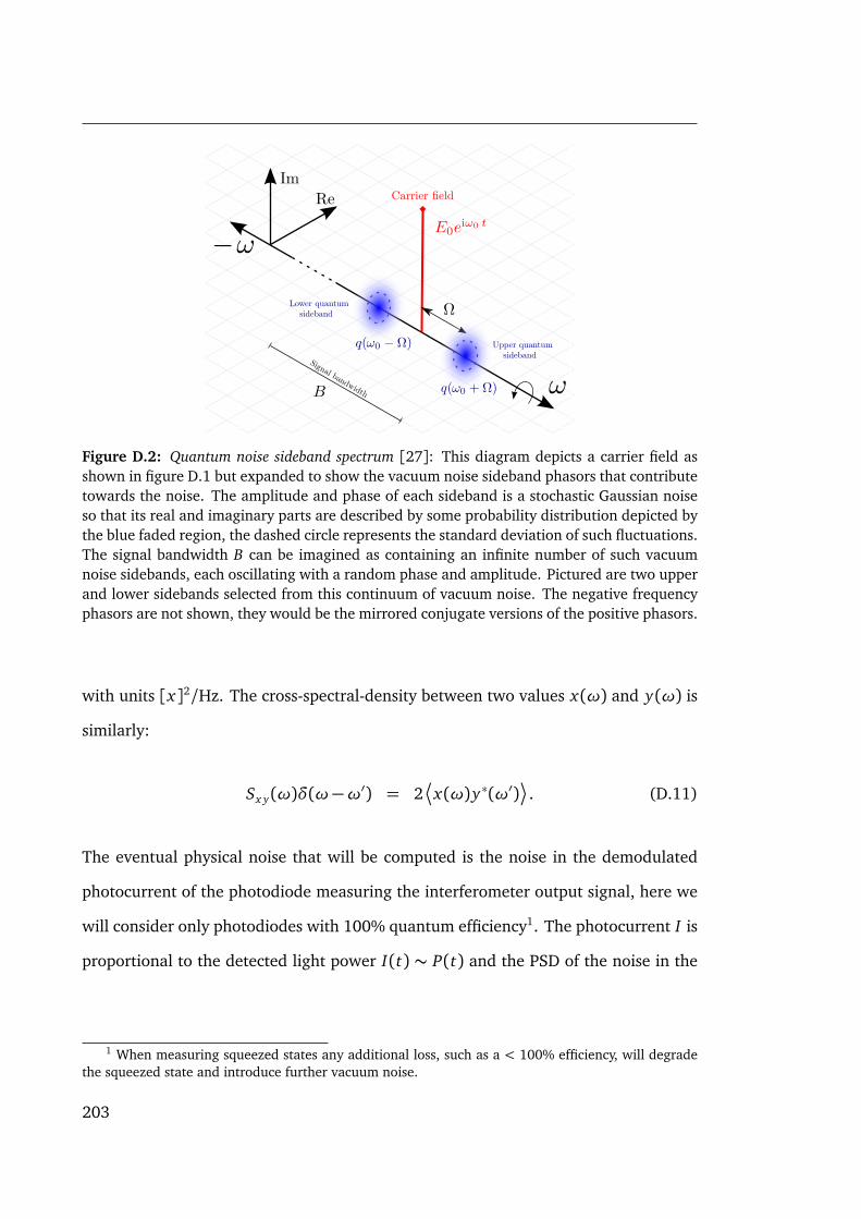
Figure D.2: Quantum noise sideband spectrum [27]: This diagram depicts a carrier field asshown in figure D.1 but expanded to show the vacuum noise sideband phasors that contributetowards the noise. The amplitude and phase of each sideband is a stochastic Gaussian noiseso that its real and imaginary parts are described by some probability distribution depicted bythe blue faded region, the dashed circle represents the standard deviation of such fluctuations.The signal bandwidth B can be imagined as containing an infinite number of such vacuumnoise sidebands, each oscillating with a random phase and amplitude. Pictured are two upperand lower sidebands selected from this continuum of vacuum noise. The negative frequencyphasors are not shown, they would be the mirrored conjugate versions of the positive phasors.
with units [x]2/Hz. The cross-spectral-density between two values x(ω) and y(ω) is
similarly:
Sx y(ω)δ(ω−ω′) = 2x(ω)y∗(ω′)
. (D.11)
The eventual physical noise that will be computed is the noise in the demodulated
photocurrent of the photodiode measuring the interferometer output signal, here we
will consider only photodiodes with 100% quantum efficiency1. The photocurrent I is
proportional to the detected light power I(t) ∼ P(t) and the PSD of the noise in the
1 When measuring squeezed states any additional loss, such as a < 100% efficiency, will degradethe squeezed state and introduce further vacuum noise.
203

D. THE QUANTUM KAT
photocurrent is:
SI(ω)δ(ω−ω′) = sI(ω)I∗(ω′)
(D.12)
The DC andω±Ω terms of the power on a photodiode for a single carrier with quantum
noise sidebands is:
P(t) = E(t)E∗(t) = |a0|2 + a∗0
∫ B
−B
q(ω0 +Ω)eiΩt dΩ
+a0
∫ B
−B
q∗(ω0 +Ω)e−iΩt dΩ+O(q2), (D.13)
terms of the order q2 are assumed to be a negligibly small contribution. The positive
half of the photocurrent spectrum for 0< Ω≤ B is given by its Fourier transform:
I(Ω) ≡ F[I(t)] = a∗0q(ω0 +Ω) + a0q∗(ω0 −Ω) (D.14)
The spectrum for frequencies in the signal bandwidth is thus defined by just quantum
noise scaled by the carrier field. From this point on for the sake of brevity we will
define the following notation without the carrier frequency, as we are only using a
single carrier for this derivation:
q(ω0 ±Ω)⇒ q± and q(ω0 ±Ω′)⇒ q′± (D.15)
Using equations D.12 and D.14, the PSD of the photocurrent is:
SI(Ω)δ(Ω−Ω′) = 2P0
q+q′∗+
+q−q′∗−
+ 2a2
0
q−q′+
∗+ 2a2
0∗q+q′−
.(D.16)
204

Now applying equations D.8 and D.9 in equation D.16 the noise PSD for a single carrier
field with vacuum noise is:
SI(ω0 ±Ω)δ(Ω−Ω′) = 2P0
q+q′∗+
+q−q′∗−
,
= P0 (ħh(ω0 +Ω) +ħh(ω0 −Ω))δ(Ω−Ω′)
SI(ω0 ±Ω) = 2P0ħhω0 (D.17)
Here we see that the quantum noise of a single carrier field does not depend on the
sideband frequency Ω. The vacuum fluctuations interfering with our carrier field pro-
duces a broadband frequency-independent noise source proportional to the carrier
power and frequency. It should also be noted that equation D.17 is the same result
as the semi-classical Schottky shot-noise equation. An interesting aspect to note here
are the differing reasons for the presence of this quantum or shot noise. The Schottky
formula derives this noise from the Poisson statistics of electrons generated in the pho-
tocurrent due to the light field power. Whereas the quantum approach reasons that
such fluctuations in the photocurrent are in fact due to vacuum noise superimposing
itself onto our light fields introducing a noise into our measurements.
Photodiode demodulation and quantum noise
The quantity that we wish to compute is the noise present in a particular photodiode’s
output of an interferometer due to quantum fluctuations in the carrier light fields. The
power spectral density (PSD) of the noise in the output current for a single carrier field
incident on a detector is described by the Schottky formula
SI = 2hf P. (D.18)
205
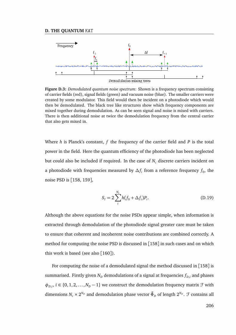
D. THE QUANTUM KAT
f+1
f0
Δf
fs
f-1
Frequency
Demodulation mixing trees
Figure D.3: Demodulated quantum noise spectrum: Shown is a frequency spectrum consistingof carrier fields (red), signal fields (green) and vacuum noise (blue). The smaller carriers werecreated by some modulator. This field would then be incident on a photodiode which wouldthen be demodulated. The black tree like structures show which frequency components aremixed together during demodulation. As can be seen signal and noise is mixed with carriers.There is then additional noise at twice the demodulation frequency from the central carrierthat also gets mixed in.
Where h is Planck’s constant, f the frequency of the carrier field and P is the total
power in the field. Here the quantum efficiency of the photodiode has been neglected
but could also be included if required. In the case of Nc discrete carriers incident on
a photodiode with frequencies measured by ∆ fi from a reference frequency f0, the
noise PSD is [158, 159],
SI = 2Nc∑i
h( f0 +∆ fi)Pi. (D.19)
Although the above equations for the noise PSDs appear simple, when information is
extracted through demodulation of the photodiode signal greater care must be taken
to ensure that coherent and incoherent noise contributions are combined correctly. A
method for computing the noise PSD is discussed in [158] in such cases and on which
this work is based (see also [160]).
For computing the noise of a demodulated signal the method discussed in [158] is
summarised. Firstly given ND demodulations of a signal at frequencies fD,i and phases
φD,i, i ∈ 0,1, 2, . . . , ND − 1 we construct the demodulation frequency matrix F with
dimensions Nc × 2ND and demodulation phase vector ~ΦD of length 2ND . F contains all
206

the frequency bins that will be mixed due to the demodulation and ~ΦD lists the total
demodulation phase of each mix.
βi j = (−1)bi/2ND− j−1c
ΦD,v =ND−1∑
i
βviφD,i (D.20)
Fuv = fc,u +ND−1∑
i
βvi fD,i (D.21)
u ∈ 0, 1,2, . . . , Nc − 1
v ∈ 0, 1,2, . . . , 2ND−1
This is based on a tree structure of the various demodulations of each carrier field.
As the above form is not particularly easy to visualise, here is an example of a double
demodulation with frequencies ∆ f and fs with 3 carriers fc = [0,−∆ f ,∆ f ] (which
are relative to a reference frequency f0) which is depicted in figure D.3:
F =
−∆ f − fs −∆ f + fs ∆ f − fs ∆ f + fs
−2∆ f − fs −2∆ f + fs − fs fs
− fs fs 2∆ f − fs 2∆ f + fs
. (D.22)
Each row in this matrix lists the frequency bins each carrier field is mixed with. Some
frequencies are unique but others are shared between multiple carrier fields. To com-
pute the noise PSD the unique frequencies contribute,
SUI (Fi j) =
h( f0 +Fi j)
4ND
ac,i
2 (D.23)
The set of Ns indices, (n, d), of the frequency bins that share multiple carrier fields
in F must be grouped together, (nk, dk)Nsk=0. For example the frequency bin − fs in
equation D.22 appears in 2 elements (1, 2), (2,0). The contribution to the noise PSD
207

D. THE QUANTUM KAT
of a shared frequency bin is then calculated by
SSI (F(n,d)) =
h( f0 +Fn0d0)
4ND
NS−1∑k=0
a∗c,nkeiΦD,dk
2
(D.24)
where the carriers are added coherently. The total noise PSD is then simply computed
as the sum of both these terms for a particular F where the set of unique frequency
indices is (mk, ek)2ND−Ns
k=0 ,
STI (F) = SS
I (F(n,d)) + SUI (F(m,e)). (D.25)
To calculate the quantum noise PSD for pure vacuum noise from each carrier field,
the above equations are all that is required. If however the interferometer contains
non-linear behaviour that squeezes the noise—such as radiation pressure effects—the
optical transfer functions from each source of quantum noise through the interferom-
eter to the photodiode outputs of interest are required. In this form these equations
are not easy to handle for large complex optical systems, an improved form is demon-
strated later.
Sources of noise are either laser noise, squeezed vacuum field inputs or optical
losses from scattering and absorption. As each source of noise is incoherent with any
other, they cannot be included in a single RHS vector input when solving the interfer-
ometer matrix—which would imply that they are coherent. Instead each noise source
must be propagated separately and combined incoherently at each output required.
The number of noise sources, Nn, scales with optical losses which can be considerable
in a realistic model of an interferometer. The total number of times the interferometer
matrix would need to be solved for is then∝ NcNn(O2 + 3O+ 2)/2, where Nc is the
number of carriers and O is the maximum order of HOM we are using in the simu-
lation; O is typically in the range 0 − 10. In simulation tools such as OPTICKLE and
208

MIST, this is the method used when modelling quantum noise. With more realistic
setups with large O the computational load is heavy. This will be referred to as the
single-input multiple-output (SIMO) method, as each source can be propagated to all
outputs with one calculation.
Next it is outlined how the noise PSD can be computed by instead propagating
all the noise sources with multiple-input single-output (MISO). In cases where noise
sources greatly outnumber the number of outputs we wish to consider this should
reduce the computational load.
Propagation of noise sidebands
As with classical audio sidebands, the propagation of quantum noise sidebands through
an interferometer is described by the matrix Mq. The matrix, Mq, is nearly identical
to that generated for describing how the classical audio sidebands propagate. Both
these matrices contain the non-linear behaviour created due to radiation pressure ef-
fects, thus describe how noise can become squeezed and how injected squeezed light
is rotated or degraded.
Consider the graphical depiction of a double demodulation as shown in figure D.3
to illustrate the problem. This shows 3 carrier fields (red), the pairs of signal sidebands
for each carrier (green) and a "sea" of vacuum fluctuations (blue); all of which are
being demodulated at the frequencies ∆ f and fs. The tree structures (black) show
how each carrier is mixed with the various signal sidebands and in the case of the
carriers at frequencies f±1 how they also mix the with pure vacuum noise.
The number of quantum noise frequency bins is typically greater than the number
of signal frequency bins, thus at first it may seem thatMq would have to include more
frequencies than Ms. However, those frequencies that are not paired with a carrier
field are typically separated from a carrier field by a frequency fs. This frequency
separation is large enough (on the order of ≈ MHz) that the beating between them
209

D. THE QUANTUM KAT
will produce negligible radiation pressure effects due to the mechanical susceptibility
of the mirrors at high frequency being∝ f −2 and reciprocally will also squeeze noise
fields negligibly.
In the case of gravitation wave detectors, the quantum noise at many MHz is far
outside the detectors designed bandwidth and thus of little interest. Therefore the
carrier-less q±s fields can be assumed to be pure incoherent vacuum noise at every
output port and do not need to be included inMq reducing the overall number of fields
to propagate to those sidebands paired with a carrier. Due to the use of a conjugated
lower sideband inMq for the computation of radiation pressure effects (see chapter 3)
the upper limit of the simulation frequency bandwidth is in practice limited. The
condition for validity of the model is that sideband frequency fs < min( fmod)/2,
i.e. that the signal/noise sideband from one carrier does not become the dominant
opposite sideband of another carrier.
MISO method
Typically for large interferometer models the number of noise sources Nn is much
greater than the number of outputs No. In these scenarios it is computationally inef-
ficient to compute the transfer function for each noise source separately by inverting
Mq. Instead a method is used for solving the transfer functions for all noise sources
for a single output which are then combined efficiently for the computation of the
noise PSD. Consider the input-output equation for the quantum sidebands, via some
rearranging and taking the expectation value we can find the co-variance matrix of
210

the output noise sidebands qout due to some injected noise sidebands qin,
Mq~qout = ~qin (D.26)
Mq~qout~q†outM†
q = ~qin~q†in (D.27)
~qout~q†out = M−1
q ~qin~q†inM−1 †
q (D.28)
⟨~qout~q†out⟩ = M−1
q ⟨~qin~q†in⟩M−1 †
q (D.29)
Vo = M−1q ViM−1 †
q (D.30)
The result here is that through one inversion of Mq and 2 matrix products we can
compute the variance-covariance matrix Vo of the noise sidebands, due to any num-
ber of input noise sources, at any output port in the interferometer. However, both
M−1q and Vo are dense matrices in practice and the requirements for holding these
in memory would be too large for most computer systems. Instead we select out the
specific values from Vo that we require to compute the noise PSD or value using an
output specific selection vectors ~siNoi=0,
Vo~si =M−1q ViM−1†
q ~si (D.31)
This can be broken down into several steps that are compatible with most modern
sparse matrix solvers [161] which typically only offer interfaces for computing the
inverted sparse matrix-vector product efficiently: First we compute the weighted con-
tribution of any noise source in the interferometer to the ith output, ~wi =M−1†q ~si; Next
we weight the actual input noise sources present, ~ni = Vi ~wi; and finally compute how
these propagate to the output,M−1q ~ni.
The obvious question is now how do we select ~si. This is entirely dependent on
what combination of variances and covariances are required. The output value must
be calculable by some combination of the noise variances with scaling factors included
211
D. THE QUANTUM KAT
in the selection vector produced by the product Vo~si. The elements of the ~si can also
be thought of as the optical carrier field on which we project the noise sidebands at
the detector. This then defines the amplitude fluctuations present in the field, thus the
amount of noise measured by the photodiode.
Selection vector: photodiode noise PSD
As previously outlined in section D the quantum noise PSD of a demodulated photo-
diode output is computed using both equations D.23 and . For the frequency bins that
are contained in the interferometer matrixMq, these equations can be represented us-
ing a specific selection vector ~spd . Computing how any number of noise sources affect
one particular photodiode’s noise PSD should then be calculable with
STI =
~s †pdVo~spd
4ND, (D.32)
which again relies on a minimal number of matrix inversions and matrix-vector prod-
ucts for fast computation. The vector ~spd should be filled with zeros apart from the
indices representing the upper and lower sidebands of all the carrier fields. The up-
per filled with the conjugate of the corresponding HOM and optical frequency carrier
amplitude and the lower with the unconjugated. This vector-matrix product will se-
lect out the variances multiple with the relevant carrier values, which is akin to both
Eq.(D) and Eq.(D.23).
This vector-matrix-vector must be equivalent to equation D.25 which is the con-
tribution to the noise PSD for both unique and shared frequencies for a particular
demodulation frequency matrix F. However, not all of the optical frequencies in Mq
are in F. These missing frequencies could also be shared or unique contributions in F,
the sets of indices for these frequencies are respectively (n′, d ′) and (m′, e′). The
total photocurrent noise PSD of a demodulated photodiode output for a generic set of
212

incident carrier fields and arbitrary optical setup is then,
STI =
~s †pdVo~spd
4ND+ SS
I (F(n′,d ′)) + SUI (F(m′,e′)). (D.33)
Source injection
An important aspect to using this method correctly is how to build the input noise
matrix, Vi. This, like the RHS vector when solving the classical interferometer matrix,
just describes what the source PSD variance and covariance between every field is; its
diagonal elements being the variances and off-diagonal elements the covariances.
Noise sources that must be considered in this input matrix are:
- Open ports
- Component losses
- Squeezing injection
- HOM scattering
The first two are straight forward. Anywhere an open port or component loss exists at a
particular node in the model the equivalent amount of noise lost must be injected back
in. Squeezed light input requires both variance and covariance between the quantum
noise sidebands of the squeezed carrier to be added. When considering HOMs it must
be stated which mode is squeezed. Currently FINESSE assumes only TEM00 is squeezed,
the rest are left as pure vacuum noise.
When HOM scattering is present in the model, noise can be both coupled between
modes or lost completely. This is due to a finite cut-off in the order of modes included.
Thus noise in one mode can be coupled to another, say in the case of a mismatched
squeezed field, or it could be lost completely if the mode it is scattered into isn’t in the
model.
213
D. THE QUANTUM KAT
This introduces a problem. To converge the results computed many HOMs would
need to be included to ensure no noise is lost, giving lower noise levels than it should;
however, this slows the simulation down dramatically. Instead it can be assumed that
whenever some scattering loss is present, pure vacuum noise is injected back in. For
any given scattering matrix, K , the total amount of lost power of the jth mode is given
by the sum of the coupling coefficients: L j = 1−∑Ni=0 |K i j|2. This states how much of
a particular mode is scattered out of the model. Ideally this value should be 0 if the
distortion is completely represented with up to order Omax .
This lost modal power can then be inserted as a scaled vacuum noise source for
each mode in the noise source matrix—just as a normal loss would. Using this tech-
nique when scattering of noise was present in the model, it was found that using
Omax = 0 gave the same result as before when using a large Omax . When squeezed
light is used enough Omax should be used to include how the squeezed states are cou-
pled between modes. Otherwise coupled squeezed light will just be replaced with
vacuum noise.
How Mq differs from Ms
Although bothMq andMs propagate the same sideband frequencies and fields through
the same interferometric setup, they differ when modelling modulator components.
WithMs the frequency bins considered are all coherent, whereas inMq the same bins
are all incoherent. Consider a single frequency bin of pure vacuum noise, similar to
that seen with demodulation, a modulator will couple more noise from other frequency
bins that match the modulator’s driving frequency into the bin of interest. At the same
time it will also take noise from this bin and couple it to others. Overall this has a net
result of leaving the same amount of vacuum noise as we began with. Thus if we make
the assumption that all incoming carrier fields have only pure vacuum noise present
all that will be present at the output is pure vacuum noise. This would not be the
214

case if squeezed fields were present on a carrier or the noise has a larger magnitude
than that of pure vacuum. However, such cases are rarely considered in gravitational
wave interferometers. Thus in FINESSE the modulator component always assumes
pure vacuum noise is input to it.
215

D. THE QUANTUM KAT
216

Appendix E
aLIGO Finesse file
Here one version of an aLIGO FINESSE is provided for reference. This file was based on
the core design file for aLIGO. It was altered to include aspects required for modelling
mode matching effects between the numerous cavities. It also contains a 16m filter
cavity with 10 dB of squeezing to provide a broadband reduction in quantum noise.
This file was developed as part of the AWC project by several members of the aLIGO
FINESSE modelling team: Paul Fulda, Charlotte Bond, Antonio Perreca, Andreas Freise
and myself.
The file is presented here to give a sense of the level of detail required to model
advanced detectors. These files and others are constantly evolving through further use
and updates to mirror the real detectors. Thus for up to date versions interested read-
ers should explore the core file folder in the aLIGO FINESSE team Git repository [29]
or those files that are uploaded to the LIGO DCC [1, 2, 3].
The usage of blocks in large FINESSE files such as this is important for organisational
and usage purposes. The blocks contain all the relevant commands for particular
subsections of the interferometer. This blocking means a several hundred line file can
be navigated with ease. It also allows a degree of automation in particular tasks as
blocks can easily be removed if that particular section of code is not required for your
217

E. ALIGO FINESSE FILE
simulation.
Code E.1 FINESSE file used for AWC simulations
#--------------------------------------------------------------------------
# aligo_IFO_maxtem4.kat (Mode matching optimized for ~18W input power)## FINESSE kat file for aligo dual recycled michelson with FP arm cavities# Tuned for use with maxtem 4 option. Includes a 16m Filter cavity and 10
dB# of squeezing## Parameters are mostly design parameters (see below).## To be used as a base file for investigations into active wavefront
control# requirements , sensing and actuation. Compatible with "awc_tools.py" file# for performing automated tasks (zero locks , plot error signals etc.)## > This is a file based on aligo_central_IFO.kat where the following# features have been added:# - Thermal lensing at ITMs (modeled as a thin lens outside# the substrate). Default value is 34.5km, corresponding to the lens# predicted at ~18W input power with 0.5ppm absorption on ITMs.# - SRM thickness;# - ROCs and lengths of PRC SRC changed following T0900043 (Table 2) to# mode match the cavities with a 34.5km thermal lens in ITMs.# - However , PR3 to BS and SR3 to BS are adjusted to maintain overall# quoted P/SRC length. These lengths have minimal effect on mode
matching.# - N.B. the thermal lens quoted in T0900043 is 50km, but this was# modeled as being inside the ITM substrate , so in this model the focal# length is adjusted by a factor 1/ nsilica.## FINESSE kat file for aLIGO dual recycled michelson with FP arm cavities.## Lengths and Rcs# - generally taken from design document T0900043 -11 unless otherwise# stated# - Schnupp asymmetry changed to 8cm (from 5cm)# - Average distance between BS and ITMX and ITMY calculated using length# of PRC , as not explicitly given (then +/- 4cm on distances to give# Schnupp asymmetry)# Reflectivities/transmission/losses# - also from T0900043 -11# - transmission of SRM changed to 35% (i.e. see T1300507 -v1)# - losses at each mirror = 37.5 ppm## Also use T1000298 -T for parameters , (design) control scheme with some# updates to match current sensing scheme.## https ://dcc.ligo.org/LIGO -L1300231# https :// awiki.ligo -wa.caltech.edu/aLIGO/Finesse %20 for%20 aLIGO# https :// alog.ligo -la.caltech.edu/aLOG/index.php?callRep =8102## DARM offset adjusted to give 147mW DC offset at 125W input power# DARM error signal derived from OMC DC power## Charlotte Bond , Daniel Brown , Paul Fulda , Antonio Perreca , Andreas
Freise# Updated on 2015 -09 -08#
218

--------------------------------------------------------------------------
%%% FTblock laser#
##########################################################################
%%% FTblock laser#
##########################################################################
l L0 125 0 n0s lmod1 1 n0 n1mod mod1 $f1 0.18 1 pm n1 n2s lmod2 1 n2 n3mod mod2 $f2 0.18 1 pm n3 n4s lmod3 1 n4 n5mod mod3 $f3 0.1 1 pm n5 n6s mod3toMC1 1 n6 nMC1in
###########################################################################
%%% FTend Laser
%%% FTblock IMC#
####################################################################################
# MC1bs1 MC1 6030u 0.6u 0 44.59 nMC1in nMC1refl nMC1trans nMC1fromMC3s sMC1toMC2 16.2405708 nMC1trans nMC2in
# MC2bs1 MC2 5.1u 9.3u 0 0.82 nMC2in nMC2refl nMC2trans dump1s sMC2toMC3 16.2405708 nMC2refl nMC3inattr MC2 Rc 27.275
# MC3bs1 MC3 5845u 0.8u 0 44.59 nMC3in nMC3refl nMC3trans nMCreturn_refls sMC3toMC1 0.465 nMC3refl nMC1fromMC3
s sMC3substrate 0.0845 $nsilica nMC3trans nMC3ARinbs2 MC3AR 0 0 0 28.9661 nMC3ARin dump nMC3ARtrans dumps sMC3ARtoIM1 0.4282 nMC3ARtrans nIM1in
#####################################################################################
%%% FTend IMC
%%% FTblock HAM2#
####################################################################################
# IM1 a.k.a. SM1bs1 IM1 0 0 0 53 nIM1in nIM1refl nIM1HRtrans dumps sIM1sub 0.02995 $nsilica nIM1HRtrans nIM1ARinbs2 IM1AR 0 0 0 33.4 nIM1ARin dump5 nIM1ARtrans dump
s IM1ARtonanoscan 3 nIM1ARtrans nIOT2Lnanoscan
#AOE1
219

E. ALIGO FINESSE FILE
s sIM1toAOE1 0.1955 nIM1refl nAOE1inlens AOE1 inf nAOE1in nAOE1trans
# IM2 a.k.a. PMMT1s sAOE1toIM2 1.0983 nAOE1trans nIM2inbs1 IM2 0 0 0 7 nIM2in nIM2refl dump dumpattr IM2 Rc 12.8
s sIM2toIM3 1.1704 nIM2refl nIM3in
# IM3 a.k.a PMMT2#s sIM2toIM3 1.1704 nIM2refl nIM3inbs1 IM3 0 0 0 7.1 nIM3in nIM3refl dump dumpattr IM3 Rc -6.24
#AOE2s sIM3toAOE2 1.041 nIM3refl nAOE2inlens AOE2 inf nAOE2in nAOE2trans
# IM4 a.k.a. SM2s sAOE2toIM4 0.134 nAOE2trans nIM4in
bs1 IM4 2400u 0 0 45 nIM4in nIM4refl nIM4trans nIM4rettranss sIM4toPRMAR 0.4135 nIM4refl nREFL
#####################################################################################
%%% FTend HAM2
%%% FTblock PR#
##########################################################################
# PRM
# AR surfacem2 PRMAR 35u 4.5u $phi_PRM nREFL nPRMARb
# Substrates sPRMsub1 0.0737 $nsilica nPRMARb nPRMHRa
# HR surfacem1 PRMHR 0.03 8.5u $phi_PRM nPRMHRa nPRMHRbattr PRMHR Rc 11.009
# Distance between PRM and PR2s lp1 $Lpr1 nPRMHRb nPR2a
# PR2bs1 PR2 250u $Mloss 0 -0.79 nPR2a nPR2b nPOP dumpattr PR2 Rc -4.545
# Distance from PR2 to PR3s lp2 $Lpr2 nPR2b nPR3a
# PR3bs1 PR3 0 $Mloss 0 0.615 nPR3a nPR3b dump dumpattr PR3 Rc 36.027
# Distance from PR3s lp3 $Lpr3 nPR3b nPRBS
###########################################################################
220

%%% FTend PR
%%% FTblock BS#
##########################################################################
# BS beamsplitter##------------------------------------------------------------## BS## ^## to IMY |## | ,’-.## | + ‘.## nYBS | ,’ :’## nPR3b | +i1 +## ----------------> ,:._ i2 ,’## from the PRC nPRBS + \ ‘-. + nXBS## ,’ i3\ ,’ --------------->## + \ + to IMX## ,’ i4.’## ‘._ ..## ‘._ ,’ |nSRBS## - |## |to the SRC## |## v##------------------------------------------------------------
bs1 BS 0.5 $Mloss $phi_BS 45 nPRBS nYBS nBSi1 nBSi3s BSsub1 0.0685 $nsilica nBSi1 nBSi2s BSsub2 0.0684 $nsilica nBSi3 nBSi4bs2 BSAR1 50u 0 0 -29.195 nBSi2 dump nXBS nPOXbs2 BSAR2 50u 0 0 29.195 nBSi4 dump nSRBS dump
###########################################################################
%%% FTend BS
%%% FTblock Yarm#
##########################################################################
# Distance from beam splitter to Y arm input mirrors ly1 5.0279 nYBS nITMY11
# Thermal lens correctionlens ITMYTL $TL_f nITMY11 nITMYTLtranss ITMYTL_null 0 nITMYTLtrans nITMYconstL_inlens ITMYconstL inf nITMYconstL_in nITMYconstL_transs ITMYTL_null2 0 nITMYconstL_trans nITMY1
# Y arm input mirrorm2 ITMYAR 20u 0 $phi_ITMY nITMY1 nITMYs1s ITMYsub 0.2 $nsilica nITMYs1 nITMYs2m1 ITMYHR 0.014 $Mloss $phi_ITMY nITMYs2 nITMY2
# Y arm lengths LYarm 3994.5 nITMY2 nETMY1
# Y arm end mirrorm1 ETMYHR 5u $Mloss $phi_ETMY nETMY1 nETMYs1s ETMYsub 0.2 $nsilica nETMYs1 nETMYs2m2 ETMYAR 500u 0 $phi_ETMY nETMYs2 nPTY
221

E. ALIGO FINESSE FILE
attr ITMYHR Rc -1934attr ETMYHR Rc 2245
attr ITMYHR mass 40attr ETMYHR mass 40
###########################################################################
%%% FTend Yarm
%%% FTblock Xarm#
##########################################################################
# Distance from beam splitter to X arm input mirrors lx1 5.0082 nXBS nITMX11
# Thermal lens correctionlens ITMXTL $TL_f nITMX11 nITMXTLtranss ITMXtl_null 0 nITMXTLtrans nITMXconstL_inlens ITMXconstL inf nITMXconstL_in nITMXconstL_transs ITMXTL_null2 0 nITMXconstL_trans nITMX1
# X arm input mirrorm2 ITMXAR 20u 0 $phi_ITMX nITMX1 nITMXs1s ITMXsub 0.2 $nsilica nITMXs1 nITMXs2m1 ITMXHR 0.014 $Mloss $phi_ITMX nITMXs2 nITMX2#m1 ITMXHR 0 $Mloss $phi_ITMX nITMXs2 nITMX2
# X arm lengths LXarm 3994.5 nITMX2 nETMX1
# X arm end mirrorm1 ETMXHR 5u $Mloss $phi_ETMX nETMX1 nETMXs1s ETMXsub 0.2 $nsilica nETMXs1 nETMXs2m2 ETMXAR 500u 0 $phi_ETMX nETMXs2 nPTX
attr ITMXHR Rc -1934attr ETMXHR Rc 2245
attr ETMXHR mass 40attr ITMXHR mass 40
###########################################################################
%%% FTend Xarm
%%% FTblock SR#
##########################################################################
# Distance to SR3s ls3 $Lsr3 nSRBS nSR3b
# SR3bs1 SR3 0 $Mloss 0 0.785 nSR3b nSR3a dump17 dumpattr SR3 Rc 35.972841
# Distance from SR3 to SR2s ls2 $Lsr2 nSR3a nSR2b
# SR2bs1 SR2 0 $Mloss 0 -0.87 nSR2b nSR2a dump dump
222
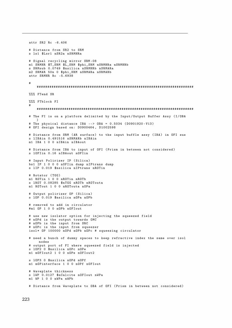
attr SR2 Rc -6.406
# Distance from SR2 to SRMs ls1 $Lsr1 nSR2a nSRMHRa
# Signal recycling mirror SRM -08m1 SRMHR $T_SRM $L_SRM $phi_SRM nSRMHRa nSRMHRbs SRMsub 0.0749 $nsilica nSRMHRb nSRMARam2 SRMAR 50n 0 $phi_SRM nSRMARa nSRMARbattr SRMHR Rc -5.6938
###########################################################################
%%% FTend SR
%%% FTblock FI#
##########################################################################
# The FI is on a platform delimited by the Input/Output Buffer Assy (I/OBA)
# The physical distance IBA --> OBA = 0.5034 (D0901920 -V13)# OFI design based on: D0900464 , D1002598
# Distance from SRM (AR surface) to the input buffle assy (IBA) in OFI suss lIBAin 0.491516 nSRMARb nIBAinm1 IBA 1 0 0 nIBAin nIBAout
# Distance from IBA to input of OFI (Prism in between not considered)s lOFIin 0.16 nIBAout nOFIin
# Input Polirizer IP (Silica)bs1 IP 1 0 0 0 nOFIin dump nIPtrans dumps lIP 0.019 $nsilica nIPtrans nROTin
# Rotator (TGG)m1 ROTin 1 0 0 nROTin nROTbs lROT 0.08285 $nTGG nROTb nROToutam1 ROTout 1 0 0 nROTouta nOPa
# Output polirizer OP (Silica)s lOP 0.019 $nsilica nOPa nOPb
# removed to add in circulator#m1 OP 1 0 0 nOPb nOFIout
# use new isolator option for injecting the squeezed field# nOPd is the output towards OMC# nOPb is the input from SRC# nOPc is the input from squeezerisol* OP 100000 nOPd nOPb nOPc # squeezing circulator
# need a bunch of dummy spaces to keep refractive index the same over isolnodes
# output port of FI where squeezed field is injecteds lOP2 0 $nsilica nOPc nOPem1 mOFIout2 1 0 0 nOPe nOFIout2
s lOP3 0 $nsilica nOPd nOPfm1 mOPinterface 1 0 0 nOPf nOFIout
# Waveplate thicknesss lWP 0.0127 $nCalcite nOFIout nWPam1 WP 1 0 0 nWPa nWPb
# Distance from Waveplate to OBA of OFI (Prism in between not considered)
223

E. ALIGO FINESSE FILE
s lOBA 0.2098563 nWPb nOBAinm1 OBA 1 0 0 nOBAin nOBAout#
##########################################################################
%%% FTend FI
%%% FTblock FilterCavity#
##########################################################################
# Mode matching settings:# Distance from BS to lens 1: d1 = 0.541093376854 m# Distance from lens1 to lens 2: d2 = 0.234279382609 m# Distance from lens1 to cavity waist: d3 = 8.22462724054 m# Focal length of lens1: f1 = -0.3 m# Focal length of lens2: f2 = 0.55 m# Distance from BS to cavity waist: D_tot = 9.0 m
s lOP_lensFC 0.541093376854 nOFIout2 nlensFC1alens lensFC1 -0.3 nlensFC1a nlensFC1bs llensFC1_lensFC2 0.234279382609 nlensFC1b nlensFC2alens lensFC2 0.55 nlensFC2a nlensFC2bs llensFC_FC 0.22462724054 nlensFC2b nIMFC2
# Confocal cavityattr IMFC Rc -15.999attr EMFC Rc 15.999const FCLength 16
# using beamsplitters for FC so no need for an isolatorbs1 IMFC 61u 0 0 0 nIMFC1 nIMFC2 nIMFC3 nIMFC4s lFC1 $FCLength nIMFC3 nEMFC1s lFC2 $FCLength nEMFC2 nIMFC4bs1 EMFC 0 0 -0.000882 0 nEMFC1 nEMFC2 dump dump
s lsqz_FC 0 nsqz nIMFC1
# finally the squeezer ...sq sqz 0 10 0 nsqz
###########################################################################
%%% FTend FilterCavity
%%% FTblock OMCpath#
##########################################################################
# (Loctions and angles based on the solid work file D1000342 -v14 give ~5%# mismatch. Thus lom1 , lom3omc have been adjusted to get ~99.7% overlap at
the OMC)# (lom1 =2.6334 , lom3omc =0.24.8 give 99% overlap at OMC)
# Distance OBA --> OM1s lom1 2.724 nOBAout nOM1a
#OM1bs1 OM1 800u $Mloss 0 2.251 nOM1a nOM1b dump dump # T is set for high
power; Loss is a guessattr OM1 Rc 4.6
# Distance OM1 --> OM2s lom2 1.395 nOM1b nOM2a
224
# OM2bs1 OM2 10u $Mloss 0 4.399 nOM2a nOM2b dump dump # T is a guessattr OM2 Rc 1.7058
# Distance OM2 --> OM3s lom3 0.631 nOM2b nOM3abs1 OM3 0.01 $Mloss 0 30.037 nOM3a nOM3b nOM3trans dump # T is a from
T1200410 -v2
# Distance OM3 --> OMC input coupler IC (AR side)s lom3omc 0.196 nOM3b nOMC_ARIC_in # By design should be ~0.31
# Distance in transmission to OM3 used for testing#s lomOM3trans 0.1 nOM3trans nOMC_ARIC2_in
###########################################################################
%%% FTend OMCpath
%%% FTblock OMC#
##########################################################################
# OMC (as built parameters: D1300507 -v1)
# Input Coupler IC (flat mirror)bs1 OMC_ARIC 1 0 0 4.004 nOMC_ARIC_in dump nOMC_ARIC_trans dumps subOMC_IC 0.01078 $nsilica nOMC_ARIC_trans nOMC_HRIC_inbs1 OMC_HRIC 0.0076 10u 0 2.7609 nOMC_HRIC_in dump nOMC_HRIC_trans
nOMC_HRICret# Distance from IC to OCs OMC_ICOC 0.2815 1 nOMC_HRIC_trans nOMC_HROC_in
# Output Coupler OC (flat mirror)bs1 OMC_HROC 0.0075 10u 0 4.004 nOMC_HROC_in nOMC_HROC_refl
nOMC_HROC_trans nOMC_HROC_rets subOMC_OC 0.01078 $nsilica nOMC_HROC_trans nOMC_AROC_inbs1 OMC_AROC 1 0 0 2.7609 nOMC_AROC_in dump nOMC_AROC_trans dump32# Distance from OC to CM1s OMC_OCCM1 0.2842 1 nOMC_HROC_refl nOMC_CM1_in
# Curved Mirror CM1bs1 OMC_CM1 36u 10u 0 4.004 nOMC_CM1_in nOMC_CM1_refl dump dump
# Distance from CM1 to CM2s OMC_CM1CM2 0.2815 1 nOMC_CM1_refl nOMC_CM2_inattr OMC_CM1 Rc 2.57321
# Curved Mirror CM2bs1 OMC_CM2 35.9u 10u 0 4.004 nOMC_CM2_in nOMC_CM2_refl dump dumpattr OMC_CM2 Rc 2.57369
# Distance from CM2 to ICs CM2OC 0.2842 1 nOMC_CM2_refl nOMC_HRICret
###########################################################################
%%% FTend OMC
%%% FTblock Lengths#
##########################################################################
# Calculate lengths of variables so Schnupp asymmetry can be changed# easily.
225
E. ALIGO FINESSE FILE
# Cavity lengthsconst Lprc 57.656#const Lprc 57.645const Lsrc 56.008const Lschnupp 0.08
# Individual lengths# PRCconst Lpr1 16.6107const Lpr2 16.1647const Lpr3 19.5381
# SRCconst Lsr1 15.7586const Lsr2 15.4435const Lsr3 19.3661
# Armsconst BSthickness 0.06873
func Laver = $Lprc - $Lpr1 - $Lpr2 - $Lpr3noplot Laver
# x length between BS and ITMfunc Lmx = $Laver + 0.5* $Lschnupp - $BSthickness * $nsilica - 0.2* $nsilicanoplot Lmxput lx1 L $Lmx
# y length between BS and ITMfunc Lmy = $Laver - 0.2* $nsilica - 0.5* $Lschnuppnoplot Lmyput ly1 L $Lmy
# Lsr3%func Lasrc = $Laver + $BSthickness * $nsilica%noplot Lasrc%func Lsr3 = $Lsrc - $Lsr1 - $Lsr2 - $Lasrc#noplot Lsr3%put ls3 L $Lsr3
###########################################################################
%%% FTend Lengths
%%% FTblock Tunings#
##########################################################################
const phi_SRM 90.0068431881324const phi_PRM 0.000212433947790268const phi_ITMX 4.36378389012253e-05const phi_ITMY -4.36378389012253e-05const phi_ETMX 0.00172458093206306const phi_ETMY -0.0017617703270198const phi_BS 0
###########################################################################
%%% FTend Tunings
%%% FTblock Constants#
##########################################################################
226
const Mloss 37.5uconst T_SRM 0.35const L_SRM 8.7u
const nsilica 1.44963098985906const nTGG 1.954const nCalcite 1.65846const f1 9099471const nf1 -9099471const f2 45497355const nf2 -45497355const f3 24000000const nf3 -24000000
const fM 36397884const nfM -36397884const fP 54596826const TL_f 34.5k
const DARM_DC_offset 0.147303#
##########################################################################
%%% FTend Constants
%%% FTblock errsigs#
##########################################################################
pd1 REFL_f1_I $f1 101 nREFLpd1 REFL_f1_Q $f1 191 nREFLpd1 REFL_f2_I $f2 14 nREFLpd1 REFL_f2_Q $f2 104 nREFLpd1 POP_f1_I $f1 101 nPOPpd1 POP_f1_Q $f1 191 nPOPpd1 POP_f2_I $f2 13 nPOPpd1 POP_f2_Q $f2 103 nPOPpd1 AS_f1_I $f1 0 nSRMARbpd1 AS_f1_Q $f1 90 nSRMARbpd1 AS_f2_I $f2 13 nSRMARbpd1 AS_f2_Q $f2 103 nSRMARb
###########################################################################
%%% FTend errsigs
%%% FTblock Powers#
##########################################################################
pd P_DC_AS nSRMARbpd P_DC_OMC nOMC_HROC_transpd PIMCtrans nREFL*pd Px nITMX2pd Py nITMY2pd Pprc nPRMHRbpd Psrc nSRMHRa*ad prc0 0 nPRMHRbad prcf1 $f1 nPRMHRbad prcf2 $f2 nPRMHRb
ad aoc0 0 nOMC_HROC_transad asc0 0 nSRMARb
227

E. ALIGO FINESSE FILE
ad asf1 $f1 nSRMARbad asf2 $f2 nSRMARbad src0 0 nSRMHRa*ad srcf1 $f1 nSRMHRa*ad srcf2 $f2 nSRMHRa*
###########################################################################
%%% FTend Powers
%%% FTblock HOMs#
##########################################################################
cav cavIMC MC2 nMC2in MC2 nMC2reflcav cavPRX PRMHR nPRMHRb ITMXHR nITMXs2cav cavPRY PRMHR nPRMHRb ITMYHR nITMYs2cav cavSRX SRMHR nSRMHRa ITMXHR nITMXs2cav cavSRY SRMHR nSRMHRa ITMYHR nITMYs2cav cavXARM ITMXHR nITMX2 ETMXHR nETMX1cav cavYARM ITMYHR nITMY2 ETMYHR nETMY1cav cavOMC OMC_HROC nOMC_HROC_refl OMC_HROC nOMC_HROC_in
maxtem 4
###########################################################################
%%% FTend HOMs
%%% FTblock locks#
##########################################################################
set PRCL_err POP_f1_I reset MICH_err POP_f2_Q reset CARM_err REFL_f1_I reset SRCL_err REFL_f2_I reset OMC_DC P_DC_OMC re
func DARM_err = $OMC_DC - $DARM_DC_offset
lock PRCL_lock $PRCL_err -2.76232377128 10ulock MICH_lock $MICH_err 12.0372824217 10ulock CARM_lock $CARM_err 0.000118716534369 10ulock DARM_lock $DARM_err -0.00577883583949 1ulock SRCL_lock $SRCL_err -4.88581756575 10u
func mMICH_lock = 0 - $MICH_lockfunc ETMX_lock = $CARM_lock + $MICH_lock + $DARM_lockfunc ETMY_lock = $CARM_lock - $MICH_lock - $DARM_lock
put* PRMHR phi $PRCL_lockput* PRMAR phi $PRCL_lock
put* ITMXHR phi $MICH_lockput* ITMXAR phi $MICH_lockput* ITMYHR phi $mMICH_lockput* ITMYAR phi $mMICH_lock
put* ETMXHR phi $ETMX_lockput* ETMXAR phi $ETMX_lock
put* ETMYHR phi $ETMY_lock
228

put* ETMYAR phi $ETMY_lock
put* SRMHR phi $SRCL_lockput* SRMAR phi $SRCL_lock
noplot PRCL_locknoplot SRCL_locknoplot MICH_locknoplot DARM_locknoplot CARM_locknoplot mMICH_locknoplot ETMX_locknoplot ETMY_lock
###########################################################################
%%% FTend locks
%%% FTblock ASWFS#
##########################################################################
s lOM3trans2ASWFSBS 0.66 nOM3trans nASWFSBSinbs ASWFSBS 0.5 0.5 0 45 nASWFSBSin nASWFSBSrefl nASWFSBStrans dump
s lASWFSBS2ASWFSA 0.1 nASWFSBSrefl nASWFSAattr lASWFSBS2ASWFSA gouy 70
s lASWFSBS2ASWFSB 0.379 nASWFSBStrans nASWFSBattr lASWFSBS2ASWFSB gouy 160
# AS WFS RF detectorspd1 ASWFSA_45I_P $f2 0 nASWFSApd1 ASWFSA_45Q_P $f2 90 nASWFSApd1 ASWFSA_36I_P $fM 15 nASWFSApd1 ASWFSA_36Q_P $fM 75 nASWFSApdtype ASWFSA_45I_P y-splitpdtype ASWFSA_45Q_P y-splitpdtype ASWFSA_36I_P y-splitpdtype ASWFSA_36Q_P y-split
pd1 ASWFSB_45I_P $f2 0 nASWFSBpd1 ASWFSB_45Q_P $f2 90 nASWFSBpd1 ASWFSB_36I_P $fM 65 nASWFSBpd1 ASWFSB_36Q_P $fM 155 nASWFSBpdtype ASWFSB_45I_P y-splitpdtype ASWFSB_45Q_P y-splitpdtype ASWFSB_36I_P y-splitpdtype ASWFSB_36Q_P y-split
const f_sig 1
# AS WFS RF detectors double demodulated at signal frequency $f_sigpd2 ASWFSA_45I_audio_P $f2 0 $f_sig max nASWFSApd2 ASWFSA_45Q_audio_P $f2 90 $f_sig max nASWFSApd2 ASWFSA_36I_audio_P $fM 0 $f_sig max nASWFSApd2 ASWFSA_36Q_audio_P $fM 90 $f_sig max nASWFSApdtype ASWFSA_45I_audio_P y-splitpdtype ASWFSA_45Q_audio_P y-splitpdtype ASWFSA_36I_audio_P y-splitpdtype ASWFSA_36Q_audio_P y-split
pd2 ASWFSB_45I_audio_P $f2 0 $f_sig max nASWFSBpd2 ASWFSB_45Q_audio_P $f2 90 $f_sig max nASWFSBpd2 ASWFSB_36I_audio_P $fM 0 $f_sig max nASWFSB
229

E. ALIGO FINESSE FILE
pd2 ASWFSB_36Q_audio_P $fM 90 $f_sig max nASWFSBpdtype ASWFSB_45I_audio_P y-splitpdtype ASWFSB_45Q_audio_P y-splitpdtype ASWFSB_36I_audio_P y-splitpdtype ASWFSB_36Q_audio_P y-split
###########################################################################
%%% FTend ASWFS
%%% FTblock commands%%% FTend commands
230

List of publications
Papers
2015 Daniel Brown et al. Optical suppression of parametric instabilities with extrac-tion cavities. 2015. In preparation
2015 Daniel Brown, Rory Smith, and Andreas Freise. Fast simulation of gaussian-modescattering for precision interferometry. Journal of Optics, Sept 2015. Submittedon 2nd of September, awaiting feedback
2015 Daniel Brown and Andreas Freise. Simulation methods for advanced interfer-ometers. In Peter Saulson and David Reitze, editors, Advanced InterferometricGravitational-wave Detectors. World Scientific, 2015. Chapter submitted in May2015
2015 C. Bond, D. Brown, A. Freise, and K. Strain. Interferometer Techniques forGravitational-Wave Detection. Living Reviews in Relativity, 13, 2015. Submit-ted as of August 2015
2013 Daniel Brown, Daniel Friedrich, Frank Brückner, Ludovico Carbone, Roman Schn-abel, and Andreas Freise. Invariance of waveguide grating mirrors to lateraldisplacement phase shifts. Opt. Lett., 38(11):1844–1846, Jun 2013
2013 Deepali Lodhia, Daniel Brown, Frank Brückner, Ludovico Carbone, Paul Fulda,Keiko Kokeyama, and Andreas Freise. Interferometer phase noise due to beammisalignment on diffraction gratings. Opt. Express, 21(24):29578–29591, Dec2013
2013 Mengyao Wang, Charlotte Bond, Daniel Brown, Frank Brückner, Ludovico Car-bone, Rebecca Palmer, and Andreas Freise. Realistic polarizing sagnac topologywith dc readout for the einstein telescope. Phys. Rev. D, 87:096008, May 2013
2013 Ludovico Carbone, Paul Fulda, Charlotte Bond, Frank Brueckner, Daniel Brown,Mengyao Wang, Deepali Lodhia, Rebecca Palmer, and Andreas Freise. The gen-eration of higher-order laguerre-gauss optical beams for high-precision interfer-ometry. (78), 2013
2012 L. Carbone, C. Bond, D. Brown, F. Brückner, K. Grover, D. Lodhia, C.M.F. Min-garelli, P. Fulda, R.J.E. Smith, R. Unwin, A. Vecchio, M. Wang, L. Whalley, and
231

A. Freise. Computer-games for gravitational wave science outreach: Black holepong and space time quest. Journal of Physics: Conference Series, 363:012057,2012
2012 P. Fulda, C. Bond, D. Brown, F. Brückner, L. Carbone, S. Chelkowski, S. Hild,K. Kokeyama, M. Wang, and A. Freise. Review of the laguerre-gauss mode tech-nology research program at birmingham. Journal of Physics: Conference Series,363:012010, 2012
Presentation, posters and technical documents
2015 Daniel Brown and Rory Smith. Presentation: Fast simulation of gaussian-modescattering for precision interferometry, 2015. DCC G1501137. Presented at theBudapest LVC meeting
2015 Paul Fulda, Daniel Brown, Charlotte Bond, Kiwamu Izumi, Lisa Barsotti, and An-dreas Freise. Simulation investigation of mode hopping in the h1 signal recyclingcavity. Technical Report T1500230, LIGO DCC, June 2015
2015 Daniel Brown, Charlotte Bond, and Andreas Freise. Finesse 2: Radiation pres-sure and the quantum kat, May 2014. DCC G1400580. Presented at GWADWTakayama
2014 Daniel Brown, Charlotte Bond, Paul Fulda, and Andreas Freise. Update on alsalignment modelling and on finesse, Jun 2014. DCC G1400622. Presented toLIGO modelling group
2013 Charlotte Bond, Paul Fulda, Daniel Brown, and Andreas Freise. Investigation ofbeam clipping in the power recycling cavity of Advanced LIGO using FINESSE.Technical Report T1300954, LIGO DCC, Nov 2013
2013 Ludovico Carbone, Daniel Brown, Charlotte Bond, Paul Fulda, and Andreas Freise.Finesse: a numerical simulation tool for optical design and detector commission-ing, Mar 2013. DCC G1300301. Poster at Bethseda LVC meeting
2013 Daniel Brown, Charlotte Bond, Mengyao Wang, Ludovico Carbone, and AndreasFreise. Modelling mirror surface distortion effects in low-loss, near-unstablefabry-perot cavities, Jul 2013. DCC G1300711. Poster at Warsaw Amaldi
2013 Daniel Brown, Charlotte Bond, and Andreas Freise. Finesse: v1.0 and beyond,May 2013. DCC G1300538. Presented at Nice LVC meeting
2013 Charlotte Bond, Daniel Brown, and Andreas Freise. Mode healing in gw inter-ferometers, Jul 2013. DCC G1300711. Poster at Warsaw Amaldi
2013 Charlotte Bond, Daniel Brown, and Andreas Freise. Mode healing in gw inter-ferometers, Jul 2013. DCC G1300711. Poster at Warsaw Amaldi
232

2013 Charlotte Bond, Paul Fulda, Daniel Brown, Andreas Freise, Keiko Kokeyama,Ludovico Carbone, Suresh Doravari, and Koji Arai. FINESSE simulation for thealignment control signal of the aligo input mode cleaner. Technical ReportT1300074, LIGO DCC, January 2013
2012 Daniel Brown and Andreas Freise. Optical simulations within and beyond theparaxial limit, May 2012. DCC G1200548. Presented at GWADW Hawaii
2012 B. Barr, A. Bell, C. Bell, C. Bond, D. Brown, F. Brueckner, L. Carbone, K. Craig,A. Cumming, S. Danilishin, K. Dooley, A. Freise, T. Fricke, P. Fulda, S. Giampsis,N. Gordon, H. Grote, G. Hammond, J. Harms, S. Hild, J. Hough, S. Huttner,R. Kumar, H. Luck, N. Lockerbie, J. Macarthur, I. Martin, P. Murray, S. Reid,S. Rowan, D. Shoemaker, B. Sorazu, K. Strain, S. Tarabrin, K. Tokmakov, andN. Voronchev. Ligo 3 strawman design, team red. Technical Report T1200046,LIGO DCC, Jan 2012
233

E. LIST OF PUBLICATIONS
234

References
[1] Charlotte Bond, Paul Fulda, Daniel Brown, Andreas Freise, Keiko Kokeyama,Ludovico Carbone, and Antonio Perreca. FINESSE input files for advanced ligo.Technical Report L1300231, LIGO DCC, August 2015.
[2] Charlotte Bond, Paul Fulda, Daniel Brown, Andreas Freise, Keiko Kokeyama,Ludovico Carbone, and Antonio Perreca. FINESSE input files for lho advancedligo. Technical Report T1300904, LIGO DCC, June 2015.
[3] Charlotte Bond, Paul Fulda, Daniel Brown, Andreas Freise, Keiko Kokeyama,Ludovico Carbone, and Antonio Perreca. FINESSE input files for llo advancedligo. Technical Report T1300901, LIGO DCC, December 2014.
[4] B.S. Sathyaprakash and Bernard F. Schutz. Physics, astrophysics and cosmologywith gravitational waves. Living Reviews in Relativity, 12(2), 2009.
[5] Daniel Brown. Stretch-and-squash, 2009. http://www.gwoptics.org/processing/stretch_and_squash/stretchandsquash.php.
[6] The LIGO Scientific Collaboration and the Virgo Collaboration. Predictionsfor the rates of compact binary coalescences observable by ground-basedgravitational-wave detectors. Classical and Quantum Gravity, 27(17):173001,2010.
[7] LIGO Scientific Collaboration and Virgo Collaboration. Narrow-band search ofcontinuous gravitational-wave signals from crab and vela pulsars in virgo vsr4data. Phys. Rev. D, 91:022004, Jan 2015.
[8] H Lück, M Hewitson, P Ajith, B Allen, P Aufmuth, C Aulbert, S Babak, R Bala-subramanian, B W Barr, S Berukoff, A Bunkowski, G Cagnoli, C A Cantley, M MCasey, S Chelkowski, Y Chen, D Churches, T Cokelaer, C N Colacino, D R MCrooks, C Cutler, K Danzmann, R J Dupuis, E Elliffe, C Fallnich, A Franzen,A Freise, I Gholami, S Goßler, A Grant, H Grote, S Grunewald, J Harms, B Hage,G Heinzel, I S Heng, A Hepstonstall, M Heurs, S Hild, J Hough, Y Itoh, G Jones,R Jones, S H Huttner, K Kötter, B Krishnan, P Kwee, M Luna, B Machenschalk,M Malec, R A Mercer, T Meier, C Messenger, S Mohanty, K Mossavi, S Mukher-jee, P Murray, G P Newton, M A Papa, M Perreur-Lloyd, M Pitkin, M V Plissi,R Prix, V Quetschke, V Re, T Regimbau, H Rehbein, S Reid, L Ribichini, D I
235
REFERENCES
Robertson, N A Robertson, C Robinson, J D Romano, S Rowan, A Rüdiger, B SSathyaprakash, R Schilling, R Schnabel, B F Schutz, F Seifert, A M Sintes, J RSmith, P H Sneddon, K A Strain, I Taylor, R Taylor, A Thüring, C Ungarelli,H Vahlbruch, A Vecchio, J Veitch, H Ward, U Weiland, H Welling, L Wen,P Williams, B Willke, W Winkler, G Woan, and R Zhu. Status of the geo600detector. Classical and Quantum Gravity, 23(8):S71–S78, 2006.
[9] Daniel Sigg and the LIGO Scientific Collaboration. Status of the ligo detectors.Classical and Quantum Gravity, 25(11):114041, 2008.
[10] The VIRGO collaboration. Virgo status. Institure of Physics, 25(18):184001(9pp), 2008.
[11] The LIGO Collaboration. Advanced ligo. Classical and Quantum Gravity,32(7):074001, 2015.
[12] The VIRGO Collaboration. Advanced virgo: a second-generation interferomet-ric gravitational wave detector. Classical and Quantum Gravity, 32(2):024001,2015.
[13] Kentaro Somiya and the KAGRA collaboration. Detector configuration of ka-gra–the japanese cryogenic gravitational-wave detector. Classical and QuantumGravity, 29(12):124007, 2012.
[14] J.-Y. Vinet, P. Hello, C. N. Man, and A. Brillet. A high accuracy method for thesimulation of non-ideal optical cavities. Journal de Physique I, 2:1287–1303,July 1992.
[15] Patrice Hello. Modele physique et simulation de l’antenne interferometrique grav-itationnelle virgo. PhD thesis, Paris-11 Univ., 91 - Orsay (France) ;, 1990.
[16] H Yamamoto, B. Bhawal, M Evans, Maros E, M Rakhmanov, and R L Jr Savage.End to end simulation program for gravitational-wave detectors. In Seiji Kawa-mura and Norikatsu Mio, editors, Graviational Wave Detection II, number 32 inFrontier Science Series. Universal Academy Press, 2000.
[17] B. Caron, L. Derome, R. Flaminio, X. Grave, F. Marion, et al. SIESTA, a timedomain, general purpose simulation program for the VIRGO experiment. As-tropart.Phys., 10:369–386, 1999.
[18] STAIC. Software tools for advanced interferometer configurations. http://www.phys.ufl.edu/LIGO/LIGO/STAIC.html, 2000. Accessed: 2014-11-18.
[19] M. Evans and Robert L. Ward. Optickle webpage. http://www.ligo.caltech.edu/~rward/Optickle/. Accessed: 2015-07-13.
[20] Gabriele Vajente. Fast modal simulation of paraxial optical systems: the mistopen source toolbox. Classical and Quantum Gravity, 30(7):075014, 2013.
236

REFERENCES
[21] Hiro Yamamoto. SIS: Stationary Interferometer Simulation. Accessed on10/08/2015: http://labcit.ligo.caltech.edu/ hiro/SIS/.
[22] Jerome Degallaix. Oscar a matlab based optical fft code. Journal of Physics:Conference Series, 228(1):012021, 2010.
[23] A Freise, G Heinzel, H Lück, R Schilling, B Willke, and K Danzmann. Frequency-domain interferometer simulation with higher-order spatial modes. Classicaland Quantum Gravity, 21(5):S1067–S1074, 2004. The program is available athttp://www.gwoptics.org/finesse.
[24] A. Freise. FINESSE webpage. http://www.gwoptics.org/finesse/. Ac-cessed: 2015-07-13.
[25] M Punturo, M Abernathy, F Acernese, B Allen, N Andersson, K Arun, F Barone,B Barr, M Barsuglia, M Beker, N Beveridge, S Birindelli, S Bose, L Bosi,S Braccini, C Bradaschia, T Bulik, E Calloni, G Cella, E Chassande Mottin,S Chelkowski, A Chincarini, J Clark, E Coccia, C Colacino, J Colas, A Cum-ming, L Cunningham, E Cuoco, S Danilishin, K Danzmann, G De Luca, R DeSalvo, T Dent, R De Rosa, L Di Fiore, A Di Virgilio, M Doets, V Fafone, P Falferi,R Flaminio, J Franc, F Frasconi, A Freise, P Fulda, J Gair, G Gemme, A Gennai,A Giazotto, K Glampedakis, M Granata, H Grote, G Guidi, G Hammond, M Han-nam, J Harms, D Heinert, M Hendry, I Heng, E Hennes, S Hild, J Hough, S Husa,S Huttner, G Jones, F Khalili, K Kokeyama, K Kokkotas, B Krishnan, M Loren-zini, H Lück, E Majorana, I Mandel, V Mandic, I Martin, C Michel, Y Minenkov,N Morgado, S Mosca, B Mours, H Müller–Ebhardt, P Murray, R Nawrodt, J Nel-son, R Oshaughnessy, C D Ott, C Palomba, A Paoli, G Parguez, A Pasqualetti,R Passaquieti, D Passuello, L Pinard, R Poggiani, P Popolizio, M Prato, P Puppo,D Rabeling, P Rapagnani, J Read, T Regimbau, H Rehbein, S Reid, L Rezzolla,F Ricci, F Richard, A Rocchi, S Rowan, A Rüdiger, B Sassolas, B Sathyaprakash,R Schnabel, C Schwarz, P Seidel, A Sintes, K Somiya, F Speirits, K Strain, S St-rigin, P Sutton, S Tarabrin, A Thüring, J van den Brand, C van Leewen, M vanVeggel, C van den Broeck, A Vecchio, J Veitch, F Vetrano, A Vicere, S Vyatchanin,B Willke, G Woan, P Wolfango, and K Yamamoto. The einstein telescope: athird-generation gravitational wave observatory. Classical and Quantum Grav-ity, 27(19):194002, 2010.
[26] A Freise, Brown D, and Bond C. FINESSE 2.0 User manual. University of Birm-ingham, 2014.
[27] C. Bond, D. Brown, A. Freise, and K. Strain. Interferometer Techniques forGravitational-Wave Detection. Living Reviews in Relativity, 13, 2015. Submittedas of August 2015.
[28] Daniel Brown and Andreas Freise. Simulation methods for advanced interfer-ometers. In Peter Saulson and David Reitze, editors, Advanced Interferometric
237

REFERENCES
Gravitational-wave Detectors. World Scientific, 2015. Chapter submitted in May2015.
[29] aLIGO FINESSE simulation team. aLIGO FINESSE git repository, 2015. Openaccess repository containing numerous LIGO based simulation data and files.http://gitmaster.atlas.aei.uni-hannover.de/aligo-finesse.
[30] S Hild, H Grote, J Degallaix, S Chelkowski, K Danzmann, A Freise, M Hewitson,J Hough, H Luck, M Prijatelj, K A Strain, J R Smith, and B Willke. Dc-readout ofa signal-recycled gravitational wave detector. Classical and Quantum Gravity,26(5):055012 (10pp), 2009.
[31] Gwinc: Gravitational wave interferometer noise calculator. Accessed on08/08/2015: http://ilog.ligo-wa.caltech.edu:7285/advligo/GWINC.
[32] A. V. Cumming, A. S. Bell, L. Barsotti, M. A. Barton, G. Cagnoli, D. Cook, L. Cun-ningham, M. Evans, G. D. Hammond, G. M. Harry, A. Heptonstall, J. Hough,R. Jones, R. Kumar, R. Mittleman, N. A. Robertson, S. Rowan, B. Shapiro, K. A.Strain, K. Tokmakov, C. Torrie, and A. A. van Veggel. Design and development ofthe advanced LIGO monolithic fused silica suspension. Classical and QuantumGravity, 29(3):035003, February 2012.
[33] S Wen, R Mittleman, K Mason, J Giaime, R Abbott, J Kern, B OÊŒReilly, R Bork,M Hammond, C Hardham, B Lantz, W Hua, D Coyne, G Traylor, H Overmier,T Evans, J Hanson, O Spjeld, M Macinnis, K Mailand, D Ottaway, D Sellers,K Carter, and P Sarin. Hydraulic external pre-isolator system for ligo. Classicaland Quantum Gravity, 31(23):235001, 2014.
[34] V. B. Braginsky, V. P. Mitrofanov, and K. V. Tokmakov. On the thermal noise fromthe violin modes of the mass suspension in gravitational wave antennae. Phys.Letters A, 186:18–20, 1993.
[35] Gabriela Gonzalez. Suspensions thermal noise in the ligo gravitational wavedetector. Class. Quantum Grav., 17:4409–4435, 2000.
[36] Jean-Yves Vinet. On special optical modes and thermal issues in advanced grav-itational wave interferometric detectors. Living Reviews in Relativity, 12(5),2009.
[37] Gregory M. Harry, Helena Armandula, Eric Black, D. R. M. Crooks, GianpietroCagnoli, Jim Hough, Peter Murray, Stuart Reid, Sheila Rowan, Peter Sneddon,Martin M. Fejer, Roger Route, and Steven D. Penn. Thermal noise from opticalcoatings in gravitational wave detectors. Appl. Opt., 45(7):1569–1574, 2006.
[38] Ke-Xun Sun, M. M. Fejer, Eric Gustafson, and Robert L. Byer. Sagnac interfer-ometer for gravitational-wave detection. Phys. Rev. Lett., 76(17):3053–3056,Apr 1996.
238

REFERENCES
[39] Mengyao Wang, Charlotte Bond, Daniel Brown, Frank Brückner, Ludovico Car-bone, Rebecca Palmer, and Andreas Freise. Realistic polarizing sagnac topologywith dc readout for the einstein telescope. Phys. Rev. D, 87:096008, May 2013.
[40] P. Kwee, C. Bogan, K. Danzmann, M. Frede, H. Kim, P. King, J. Pöld, O. Puncken,R. L. Savage, F. Seifert, P. Wessels, L. Winkelmann, and B. Willke. Stabilizedhigh-power laser system for the gravitational wave detector advanced ligo. Opt.Express, 20(10):10617–10634, May 2012.
[41] Patrick Kwee. Laser Characterization and Stabilization for Precision Interferom-etry. PhD thesis, Universitat Hannover, 2010.
[42] Benno Willke. Pre-stabilized laser design requirements. Technical ReportT050036, LIGO DCC, Feb 2009.
[43] Daniel Brown and Andreas Freise. Optical simulations within and beyond theparaxial limit, May 2012. DCC G1200548. Presented at GWADW Hawaii.
[44] A.E. Siegman. LASERS. University Science Books, 1986. See also: Errata List forLASERS, http://www.stanford.edu/~siegman/lasers_book_errata.pdf.
[45] Herwig Kogelnik. On the propagation of Gaussian beams of light through lens-like media including those with a loss or gain variation. Appl. Opt., 4(12):1562–1569, 1965.
[46] Kenneth A. Strain, Guido Müller, Tom Delker, David H. Reitze, David B. Tanner,James E. Mason, Phil A. Willems, Daniel A. Shaddock, Malcolm B. Gray, ConorMow-Lowry, and David E. McClelland. Sensing and control in dual-recyclinglaser interferometer gravitational-wave detectors. Appl. Opt., 42(7):1244–1256, Mar 2003.
[47] A. Jeffrey and D. Zwillinger. Table of Integrals, Series, and Products. Table ofIntegrals, Series, and Products Series. Elsevier Science, 2007.
[48] Charlote Bond, Daniel Brown, and Andreas Freise. Interferometer responses togravitational waves: Comparing finesse simulations and analytical solutions.Technical Report T1300190, LIGO DCC, March 2013.
[49] Koji Arai. aligo output mode cleaner: Overview of the realtime model andscreens. Technical Report E1500161, LIGO DCC, March 2015.
[50] GariLynn Billingsley. Etm08 end test mass final polishing data package. Tech-nical Report C1000486, LIGO DCC, Feb 2014.
[51] G. Billingsley. LIGO core optics reference page. https://galaxy.ligo.caltech.edu/optics/. Accessed: 2015-07-13.
239

REFERENCES
[52] Charlotte Bond, Paul Fulda, Daniel Brown, and Andreas Freise. Investigation ofbeam clipping in the power recycling cavity of Advanced LIGO using FINESSE.Technical Report T1300954, LIGO DCC, Nov 2013.
[53] Charlotte Zoë Bond. How to stay in shape: overcoming beam and mirror dis-tortions in advanced gravitational wave interferometers. July 2014.
[54] F. Bayer-Helms. Coupling coefficients of an incident wave and the modes ofspherical optical resonator in the case of mismatching and misalignment. Appl.Opt., 23:1369–1380, May 1984.
[55] J. Y. Vinet and the Virgo Collaboration. The Virgo Book of Physics: Optics andRelated Topics. Virgo, 2001.
[56] Christopher L Mueller. TECHNIQUES FOR RESONANT OPTICAL INTERFEROM-ETRY WITH APPLICATIONS TO THE ADVANCED LIGO GRAVITATIONAL WAVEDETECTORS. PhD thesis, UNIVERSITY OF FLORIDA, 2014.
[57] Anthony E. Siegman and R. Arrathoon. Modes in unstable optical resonatorsand lens waveguides. Quantum Electronics, IEEE Journal of, 3(4):156–163, Apr1967.
[58] Koji Arai. On the accumulated round-trip gouy phase shift for a general opticalcavity. Technical Report T1300189, LIGO DCC, March 2013.
[59] M.A. Arain and G. Mueller. Design of the advanced ligo recycling cavities. OpticsExpress, Vol. 16, Issue 14:10018–10032, 2008.
[60] Rich Abbott, Rana Adhikari, Stefan Ballmer, Lisa Barsotti, Matt Evans, Pe-ter Fritschel, Valera Frolov, Guido Mueller, Bram Slagmolen, and Sam Wald-man. Advanced ligo length sensing and control final design. Technical ReportT1000298, LIGO DCC, June 2010.
[61] J. Mizuno, K.A. Strain, P.G. Nelson, J.M. Chen, R. Schilling, A. Rüdiger, W. Win-kler, and K. Danzmann. Resonant sideband extraction: a new configuration forinterferometric gravitational wave detectors. Physics Letters A, 175(5):273 –276, 1993.
[62] Lisa Barsotti and Matt Evans. Modeling of alignment sensing and control foradvanced ligo. Technical Report T0900511, LIGO DCC, June 2010.
[63] Harbir Antil, ScottE. Field, Frank Herrmann, RicardoH. Nochetto, and ManuelTiglio. Two-step greedy algorithm for reduced order quadratures. Journal ofScientific Computing, 57(3):604–637, 2013.
[64] Daniel Brown, Rory Smith, and Andreas Freise. Fast simulation of gaussian-mode scattering for precision interferometry. Journal of Optics, Sept 2015.Submitted on 2nd of September, awaiting feedback.
240

REFERENCES
[65] T. Hahn. Cuba—a library for multidimensional numerical integration. ComputerPhysics Communications, 168(2):78 – 95, 2005.
[66] Priscilla Canizares, Scott E. Field, Jonathan Gair, Vivien Raymond, Rory Smith,and Manuel Tiglio. Accelerated gravitational wave parameter estimation withreduced order modeling. Phys. Rev. Lett., 114:071104, Feb 2015.
[67] Daniel Brown and Andreas Freise. PYKAT webpage. http://www.gwoptics.org/pykat/, 2015. Accessed: 2015-07-13.
[68] Y. Maday, N. C. Nguyen, A. T. Patera, and S. H. Pau. A general multipurposeinterpolation procedure: the magic points. Communications on Pure and AppliedAnalysis, 8:383–404, 2009.
[69] A. Ralston and P. Rabinowitz. A First Course in Numerical Analysis. Dover bookson mathematics. Dover Publications, 2001.
[70] Maxime Barrault, Yvon Maday, Ngoc Cuong Nguyen, and Anthony T. Patera.An ‘empirical interpolation’ method: application to efficient reduced-basis dis-cretization of partial differential equations. Comptes Rendus Mathematique,339(9):667 – 672, 2004.
[71] Jan S. Hesthaven, Benjamin Stamm, and Shun Zhang. Efficient greedy algo-rithms for high-dimensional parameter spaces with applications to empiricalinterpolation and reduced basis methods. ESAIM: Mathematical Modelling andNumerical Analysis, 48:259–283, 1 2014.
[72] Max D. Gunzburger, Janet S. Peterson, and John N. Shadid. Reduced-ordermodeling of time-dependent PDEs with multiple parameters in the boundarydata. Computer Methods in Applied Mechanics and Engineering, 196(4–6):1030– 1047, 2007.
[73] B. S. Kirk, J. W. Peterson, R. H. Stogner, and G. F. Carey. libMesh: A C++Library for Parallel Adaptive Mesh Refinement/Coarsening Simulations. Engi-neering with Computers, 22(3–4):237–254, 2006.
[74] William H. Press, Saul A. Teukolsky, William T. Vetterling, and Brian P. Flan-nery. Numerical Recipes 3rd Edition: The Art of Scientific Computing. CambridgeUniversity Press, New York, NY, USA, 3 edition, 2007.
[75] Kendall Atkinson. An Introduction to Numerical Analysis. Wiley, 2 edition.
[76] Tor Øvstedal Aanonsen. Empirical interpolation with application to reducedbasis approximations. 2009.
[77] FINESSE input files for Advanced LIGO. https://dcc.ligo.org/LIGO-L1300231, 2015. Accessed: 2015-07-13.
241

REFERENCES
[78] Daniel Brown et al. Optical suppression of parametric instabilities with extrac-tion cavities. 2015. In preparation.
[79] P. Meystre, J. D. McCullen, E. Vignes, and E. M. Wright. Theory of radiation-pressure-driven interferometers. J. Opt. Soc. Am. B, 2(11):1830–1840, Nov1985.
[80] O Miyakawa and H Yamamoto. Lock acquisition studies for advanced interfer-ometers. Journal of Physics: Conference Series, 122(1):012024, 2008.
[81] M. Evans, N. Mavalvala, P. Fritschel, R. Bork, B. Bhawal, R. Gustafson, W. Kells,M. Landry, D. Sigg, R. Weiss, S. Whitcomb, and H. Yamamoto. Lock acquisitionof a gravitational-wave interferometer. Opt. Lett., 27(8):598–600, Apr 2002.
[82] B. Bhawal, M. Evans, E. Maros, M. Rakhmanov, R. L. Savage, Jr., H. Yamamoto,G. Cella, and S. Klimenko. End-to-End simulation program for interferometricgravitational wave detectors. In APS Meeting Abstracts, page 20001, April 2000.
[83] M. Evans, Mathematics California Institute of Technology. Division of Physics,and Astronomy. Lock acquisition in resonant optical interferometers. CIT theses.California Institute of Technology, 2002.
[84] J. A. Sidles and D. Sigg. Optical torques in suspended Fabry Perot interferom-eters. Physics Letters A, 354:167–172, May 2006.
[85] Katherine L. Dooley, Lisa Barsotti, Rana X. Adhikari, Matthew Evans, To-bin T. Fricke, Peter Fritschel, Valera Frolov, Keita Kawabe, and Nicolás Smith-Lefebvre. Angular control of optical cavities in a radiation-pressure-dominatedregime: the enhanced ligo case. J. Opt. Soc. Am. A, 30(12):2618–2626, Dec2013.
[86] Matthew Evans, Slawek Gras, Peter Fritschel, John Miller, Lisa Barsotti, De-nis Martynov, Aidan Brooks, Dennis Coyne, Rich Abbott, Rana X. Adhikari, KojiArai, Rolf Bork, Bill Kells, Jameson Rollins, Nicolas Smith-Lefebvre, Gabriele Va-jente, Hiroaki Yamamoto, Carl Adams, Stuart Aston, Joseph Betzweiser, ValeraFrolov, Adam Mullavey, Arnaud Pele, Janeen Romie, Michael Thomas, KeithThorne, Sheila Dwyer, Kiwamu Izumi, Keita Kawabe, Daniel Sigg, Ryan Derosa,Anamaria Effler, Keiko Kokeyama, Stefan Ballmer, Thomas J. Massinger, AlexaStaley, Matthew Heinze, Chris Mueller, Hartmut Grote, Robert Ward, EleanorKing, David Blair, Li Ju, and Chunnong Zhao. Observation of parametric insta-bility in advanced ligo. Phys. Rev. Lett., 114:161102, Apr 2015.
[87] V. B. Braginsky, S. E. Strigin, and S. P. Vyatchanin. Parametric oscillatory insta-bility in Fabry-Perot interferometer. Physics Letters A, 287:331–338, September2001.
[88] C Zhao, D G Blair, P Barrigo, J Degallaix, J-C Dumas, Y Fan, S Gras, L Ju, B Lee,S Schediwy, Z Yan, D E McClelland, S M Scott, M B Gray, A C Searle, S Gossler,
242

REFERENCES
B J J Slagmolen, J Dickson, K McKenzie, C Mow-Lowry, A Moylan, D Rabeling,J Cumpston, K Wette, J Munch, P J Veitch, D Mudge, A Brooks, and D Hosken.Gingin high optical power test facility. Journal of Physics: Conference Series,32(1):368, 2006.
[89] Thomas Corbitt, David Ottaway, Edith Innerhofer, Jason Pelc, and Nergis Maval-vala. Measurement of radiation-pressure-induced optomechanical dynamics ina suspended fabry-perot cavity. Physical Review A (Atomic, Molecular, and Opti-cal Physics), 74(2):021802, 2006.
[90] John Miller. On Non-Gaussian Beams and Optomechanical Parametric Instabil-ities in Interferometric Gravitational Wave Detectors. PhD thesis, University ofGlasgow, 2010.
[91] Luke Williams. Dimensions for advanced ligo fused silica test masses. TechnicalReport T040199, LIGO DCC, Feb 2004.
[92] Brian Schwarz and Mark Richar Dson. Scaling mode shapes obtained fromoperating data. Technical report, International Modal Analysis Conf. (IMACXXIV), February, 2003.
[93] Sondipon Adhikari. Damping Models for Structural Vibration. PhD thesis, Cam-bridge University, Cambridge University, 2000.
[94] R Nawrodt, A Zimmer, T Koettig, C Schwarz, D Heinert, M Hudl, R Neubert,M Thük, S Nietzsche, W Vodel, P Seidel, and A Tännermann. High mechanicalq-factor measurements on silicon bulk samples. Journal of Physics: ConferenceSeries, 122(1):012008, 2008.
[95] M. Evans, L. Barsotti, and P. Fritschel. A general approach to optomechanicalparametric instabilities. Physics Letters A, 374(4):665 – 671, 2010.
[96] Thomas Corbitt. Private email from T. Corbitt, August 2015. Requested data onthe Q-factor of the mechanical mode from Thomas Cobitt, his reply: "I recallthe Q of the drumhead to be in the 5e5 to 1e6 range".
[97] Thomas Randall Corbitt. Quantum Noise and Radiation Pressure Effects in HighPower Optical Interferometers. PhD thesis, MASSACHUSETTS INSTITUTE OFTECHNOLOGY, 2008.
[98] S Gras, C Zhao, D G Blair, and L Ju. Parametric instabilities in advanced gravita-tional wave detectors. Classical and Quantum Gravity, 27(20):205019, 2010.
[99] V. B. Braginsky, S. E. Strigin, and S. P. Vyatchanin. Analysis of parametric os-cillatory instability in power recycled LIGO interferometer. Physics Letters A,305:111–124, December 2002.
243

REFERENCES
[100] A. G. Gurkovsky, S. E. Strigin, and S. P. Vyatchanin. Analysis of parametricoscillatory instability in signal recycled LIGO interferometer. Physics Letters A,362:91–99, February 2007.
[101] S.E. Strigin. The effect of parametric oscillatory instability in a fabry-perot cav-ity of the einstein telescope. Optics and Spectroscopy, 112(3):373–376, 2012.
[102] S.E. Strigin. Suppression of parametric oscillatory instability in third generationgravitational wave detectors. Physics Letters A, 379(2829):1671 – 1674, 2015.
[103] C. Zhao, L. Ju, J. Degallaix, S. Gras, and D. G. Blair. Parametric Instabilitiesand Their Control in Advanced Interferometer Gravitational-Wave Detectors.Physical Review Letters, 94(12):121102–+, April 2005.
[104] John Miller, Matthew Evans, Lisa Barsotti, Peter Fritschel, Myron MacInnis,Richard Mittleman, Brett Shapiro, Jonathan Soto, and Calum Torrie. Damp-ing parametric instabilities in future gravitational wave detectors by means ofelectrostatic actuators. Physics Letters A, 375(3):788 – 794, 2011.
[105] S.E. Strigin, D.G. Blair, S. Gras, and S.P. Vyatchanin. Numerical calculationsof elastic modes frequencies for parametric oscillatory instability in advancedLIGO interferometer. Physics Letters A, 372(35):5727 – 5731, 2008.
[106] S. Gras, D. G. Blair, and L. Ju. Opto-acoustic interactions in gravitationalwave detectors: Comparing flat-top beams with Gaussian beams. Phys. Rev.D, 81(4):042001–+, February 2010.
[107] Charlotte Bond, Paul Fulda, Daniel Brown, Andreas Freise, Keiko Kokeyama,Ludovico Carbone, Suresh Doravari, and Koji Arai. FINESSE simulation for thealignment control signal of the aligo input mode cleaner. Technical ReportT1300074, LIGO DCC, January 2013.
[108] LIGO Lab. aLIGO logbooks, 2015. alog.ligo-wa.caltech.edu and alog.ligo-la.caltech.edu.
[109] Daniel Brown, Paul Fulda, Antonio Perreca, Andreas Freise, Anna Green, andDaniel Toyra. Active wavefront control simulation project update. TechnicalReport G1501039, LIGO DCC, August 2015.
[110] Paul Fulda, Charlotte Bond, Daniel Brown, and Andreas Freise. Mode matchingmeasurement and modeling update. Technical Report G1400381, LIGO DCC,March 2014.
[111] Kiwamu Izumi et al. Drmi locked for the first time. Technical Report 14002,LIGO LHO Logbook, September 2014.
[112] Paul Fulda, Daniel Brown, Charlotte Bond, Kiwamu Izumi, Lisa Barsotti, andAndreas Freise. Simulation investigation of mode hopping in the h1 signalrecycling cavity. Technical Report T1500230, LIGO DCC, June 2015.
244
REFERENCES
[113] Paul Fulda, Daniel Brown, and Andreas Freise. Sensing and control problems inlow finesse cavities, or "how (not) to hop". Technical Report G1500645, LIGODCC, May 2015.
[114] Luke Williams. Aligo io h1 master coordinate list. Technical Report E1200616,LIGO DCC, August 2013.
[115] Shelia Dwyer et al. Drmi locking tonight. Technical Report 14027, LIGO LHOLogbook, September 2014.
[116] Evan Hall et al. Drmi1f characterization (no arms). Technical Report 15362,LIGO LHO Logbook, December 2014.
[117] Chris Mueller and Lisa Barsotti. Mode matching investigations at llo. TechnicalReport G1300909, LIGO DCC, Sept 2013.
[118] GariLynn Billingsley. Itm04 input test mass final polishing data package. Tech-nical Report C1000472, LIGO DCC, May 2011.
[119] GariLynn Billingsley. Itm08 input test mass final polishing data package. Tech-nical Report C1000476, LIGO DCC, May 2011.
[120] Lisa Barsotti et al. Omc mismatching. Technical Report 8192, LIGO LLO Log-book, August 2013.
[121] Jerome. Compensation of strong thermal lensing in advanced interferometricgravitational waves detectors. PhD thesis, The University of Western Australia,2006.
[122] R. Lawrence, M. Zucker, P. Fritschel, P. Marfuta, and D. Shoemaker. Adaptivethermal compensation of test masses in advanced LIGO. Classical and QuantumGravity, 19:1803–1812, April 2002.
[123] Luke Williams. Aligo io l1 master coordinate list. Technical Report E1200274,LIGO DCC, Dec 2012.
[124] Aidan Brooks, Antonio Perreca, Lisa Barsotti, and Paul Fulda. Active wavefrontcontrol, or the story of adaptive higher order mode control (ad hoc). TechnicalReport G1500372, LIGO DCC, March 2015.
[125] Aidan Brooks, Antonio Perreca, Lisa Barsotti, Paul Fulda, Rana Adhikari, andStefan Ballmer. Active wavefront control roadmap. Technical Report T1500188,LIGO DCC, March 2015.
[126] H. J. Kimble, Y. Levin, A. B. Matsko, K. S. Thorne, and S. P. Vyatchanin. Conver-sion of conventional gravitational-wave interferometers into quantum nonde-molition interferometers by modifying their input and/or output optics. Physi-cal Review D, 65(2):022002–+, January 2002.
245

REFERENCES
[127] M. Evans, L. Barsotti, J. Harms, P. Kwee, and H. Miao. Realistic filter cavitiesfor advanced gravitational wave detectors. ArXiv, 2013.
[128] P. Kwee, J. Miller, T. Isogai, L. Barsotti, and M. Evans. Decoherence and degra-dation of squeezed states in quantum filter cavities. Phys. Rev. D, 90:062006,Sep 2014.
[129] Daniel Brown, Daniel Friedrich, Frank Brückner, Ludovico Carbone, RomanSchnabel, and Andreas Freise. Invariance of waveguide grating mirrors to lat-eral displacement phase shifts. Opt. Lett., 38(11):1844–1846, Jun 2013.
[130] Daniel Brown. Finite-difference time-domain analysis of diffraction and waveg-uide coating displacement phase shifts. Master’s thesis, University of Birming-ham, School of Physics and Astronomy, 2010.
[131] Helge Müller-Ebhardt, Henning Rehbein, Roman Schnabel, Karsten Danzmann,and Yanbei Chen. Entanglement of macroscopic test masses and the standardquantum limit in laser interferometry. Phys. Rev. Lett., 100:013601, Jan 2008.
[132] Kenji Numata, Amy Kemery, and Jordan Camp. Thermal-noise limit in the fre-quency stabilization of lasers with rigid cavities. Phys. Rev. Lett., 93:250602,Dec 2004.
[133] Gregory M Harry, Andri M Gretarsson, Peter R Saulson, Scott E Kittelberger,Steven D Penn, William J Startin, Sheila Rowan, Martin M Fejer, D R M Crooks,Gianpietro Cagnoli, Jim Hough, and Norio Nakagawa. Thermal noise in in-terferometric gravitational wave detectors due to dielectric optical coatings.Classical and Quantum Gravity, 19(5):897, 2002.
[134] Simon Chelkowski, Stefan Hild, and Andreas Freise. Prospects of higher-orderlaguerre-gauss modes in future gravitational wave detectors. Physical Review D(Particles, Fields, Gravitation, and Cosmology), 79(12):122002, 2009.
[135] Ke-Xun Sun and Robert L. Byer. All-reflective michelson, sagnac, and fabry–perot interferometers based on grating beam splitters. Opt. Lett., 23(8):567–569, Apr 1998.
[136] A. Bunkowski, O. Burmeister, D. Friedrich, K. Danzmann, and R. Schnabel. Highreflectivity grating waveguide coatings for 1064 nm. Classical and QuantumGravity, 23:7297–7303, December 2006.
[137] Y. Levin. Internal thermal noise in the LIGO test masses: A direct approach.Phys. Rev. D, 57:659–663, January 1998.
[138] S. Wise, V. Quetschke, A. J. Deshpande, G. Mueller, D. H. Reitze, D. B. Tanner,B. F. Whiting, Y. Chen, A. Tünnermann, E. Kley, and T. Clausnitzer. Phase Effectsin the Diffraction of Light: Beyond the Grating Equation. Physical Review Letters,95(1):013901–+, June 2005.
246

REFERENCES
[139] Deepali Lodhia, Daniel Brown, Frank Brückner, Ludovico Carbone, Paul Fulda,Keiko Kokeyama, and Andreas Freise. Interferometer phase noise due to beammisalignment on diffraction gratings. Opt. Express, 21(24):29578–29591, Dec2013.
[140] A. Freise, A. Bunkowski, and R. Schnabel. Phase and alignment noise in gratinginterferometers. New Journal of Physics, 9:433–+, December 2007.
[141] Frank Brückner, Tina Clausnitzer, Oliver Burmeister, Daniel Friedrich, Ernst-Bernhard Kley, Karsten Danzmann, Andreas Tünnermann, and Roman Schn-abel. Monolithic dielectric surfaces as new low-loss light-matter interfaces.Opt. Lett., 33(3):264–266, 2008.
[142] Deepali Lodhia. Investigations into phase effects from diffracted gaussianbeams for high-precision interferometry. July 2013.
[143] Allen Taflove and Susan C. Hagness. Computational Electrodynamics: The Finite-Difference Time-Domain Method, Third Edition. Artech House Publishers, 3 edi-tion, June 2005.
[144] Petr Sysel and Pavel Rajmic. Goertzel algorithm generalized to non-integermultiples of fundamental frequency. EURASIP Journal on Advances in SignalProcessing, 2012:1–8, 2012. 10.1186/1687-6180-2012-56.
[145] S. Kroker, E.-B. Kley, and A. Tunnermann. Thermal noise of silicon basedgrating reflectors for high-precision metrology. In Metrology for Aerospace(MetroAeroSpace), 2014 IEEE, pages 523–527, May 2014.
[146] S. Kroker, T. Käsebier, E.-B. Kley, and A. Tünnermann. Investigation on theangular dependent reflectance of coupled high-contrast gratings. In Society ofPhoto-Optical Instrumentation Engineers (SPIE) Conference Series, volume 8995of Society of Photo-Optical Instrumentation Engineers (SPIE) Conference Series,page 0, February 2014.
[147] S Leavey, B W Barr, A S Bell, N Gordon, C Gräf, S Hild, S H Huttner, E-B Kley,S Kroker, J Macarthur, C Messenger, M Pitkin, B Sorazu, K Strain, and A Tün-nermann. Upper limit to the transverse to longitudinal motion coupling of awaveguide mirror. Classical and Quantum Gravity, 32(17):175005, 2015.
[148] Ayaka Kumeta, Charlotte Bond, and Kentaro Somiya. Design study of the kagraoutput mode cleaner. Optical Review, 22(1):149–152, 2015.
[149] H Wittel, H Lück, C Affeldt, K L Dooley, H Grote, J R Leong, M Prijatelj,E Schreiber, J Slutsky, K Strain, M Was, B Willke, and K Danzmann. Ther-mal correction of astigmatism in the gravitational wave observatory geo-600.Classical and Quantum Gravity, 31(6):065008, 2014.
247

REFERENCES
[150] C Bond, P Fulda, L Carbone, K Kokeyama, and A Freise. The effect of mirrorsurface distortions on higher order Laguerre-Gauss modes. Journal of Physics:Conference Series, 363:012005, 2012.
[151] B Sorazu, P J Fulda, B W Barr, A S Bell, C Bond, L Carbone, A Freise, S Hild,S H Huttner, J Macarthur, and K A Strain. Experimental test of higher-orderlaguerre-gauss modes in the 10 m glasgow prototype interferometer. Classicaland Quantum Gravity, 30(3):035004, 2013.
[152] C Grëf, B W Barr, A S Bell, F Campbell, A V Cumming, S L Danilishin, N AGordon, G D Hammond, J Hennig, E A Houston, S H Huttner, R A Jones, S SLeavey, H LÃŒck, J Macarthur, M Marwick, S Rigby, R Schilling, B Sorazu,A Spencer, S Steinlechner, K A Strain, and S Hild. Design of a speed meterinterferometer proof-of-principle experiment. Classical and Quantum Gravity,31(21):215009, 2014.
[153] Jordan Clarke, Haoyu Wang, Daniel Brown, and Andreas Freise. Revisting side-bands of sidebands in finesse. Technical Report T1300986, LIGO DCC, Dec2013.
[154] Andreas Freise, Charlotte Bond, and Daniel Brown. SIMTOOLS webpage. http://www.gwoptics.org/simtools/, 2015. Accessed: 2015-07-13.
[155] C. M. Caves and B. L. Schumaker. New formalism for two-photon quantumoptics. I - Quadrature phases and squeezed states. II - Mathematical foundationand compact notation. Physical Review A, 31:3068–3111, May 1985.
[156] Hans-A. Bachor and Peter J. Manson. Practical implications of quantum noise.Journal of Modern Optics, 37(11):1727–1740, 1990.
[157] B. J. Meers and K. A. Strain. Modulation, signal, and quantum noise in inter-ferometers. Phys. Rev. A, 44:4693–4703, October 1991.
[158] J. Harms, P. Cochrane, and A. Freise. Quantum-noise power spectrum of fieldswith discrete classical components. Phys. Rev. A, 76(2):023803–+, August2007.
[159] C.M. Caves. Quantum-mechanical noise in an interferometer. Phys. Rev. D,23:1693–1708, 1981.
[160] Malik Rakhmanov. Demodulation of intensity and shot noise in the opticalheterodyne detection of laser interferometers for gravitational waves. Appl.Opt., 40(36):6596–6605, Dec 2001.
[161] T.A. Davis. Direct Methods for Sparse Linear Systems, volume 2 of Fundamentalsof Algorithms. SIAM, Philadelphia, 2006.
248

REFERENCES
[162] Ludovico Carbone, Paul Fulda, Charlotte Bond, Frank Brueckner, Daniel Brown,Mengyao Wang, Deepali Lodhia, Rebecca Palmer, and Andreas Freise. The gen-eration of higher-order laguerre-gauss optical beams for high-precision inter-ferometry. (78), 2013.
[163] L. Carbone, C. Bond, D. Brown, F. Brückner, K. Grover, D. Lodhia, C.M.F. Min-garelli, P. Fulda, R.J.E. Smith, R. Unwin, A. Vecchio, M. Wang, L. Whalley, andA. Freise. Computer-games for gravitational wave science outreach: Black holepong and space time quest. Journal of Physics: Conference Series, 363:012057,2012.
[164] P. Fulda, C. Bond, D. Brown, F. Brückner, L. Carbone, S. Chelkowski, S. Hild,K. Kokeyama, M. Wang, and A. Freise. Review of the laguerre-gauss modetechnology research program at birmingham. Journal of Physics: ConferenceSeries, 363:012010, 2012.
[165] Daniel Brown and Rory Smith. Presentation: Fast simulation of gaussian-modescattering for precision interferometry, 2015. DCC G1501137. Presented at theBudapest LVC meeting.
[166] Daniel Brown, Charlotte Bond, and Andreas Freise. Finesse 2: Radiation pres-sure and the quantum kat, May 2014. DCC G1400580. Presented at GWADWTakayama.
[167] Daniel Brown, Charlotte Bond, Paul Fulda, and Andreas Freise. Update on alsalignment modelling and on finesse, Jun 2014. DCC G1400622. Presented toLIGO modelling group.
[168] Ludovico Carbone, Daniel Brown, Charlotte Bond, Paul Fulda, and AndreasFreise. Finesse: a numerical simulation tool for optical design and detectorcommissioning, Mar 2013. DCC G1300301. Poster at Bethseda LVC meeting.
[169] Daniel Brown, Charlotte Bond, Mengyao Wang, Ludovico Carbone, and An-dreas Freise. Modelling mirror surface distortion effects in low-loss, near-unstable fabry-perot cavities, Jul 2013. DCC G1300711. Poster at WarsawAmaldi.
[170] Daniel Brown, Charlotte Bond, and Andreas Freise. Finesse: v1.0 and beyond,May 2013. DCC G1300538. Presented at Nice LVC meeting.
[171] Charlotte Bond, Daniel Brown, and Andreas Freise. Mode healing in gw inter-ferometers, Jul 2013. DCC G1300711. Poster at Warsaw Amaldi.
[172] B. Barr, A. Bell, C. Bell, C. Bond, D. Brown, F. Brueckner, L. Carbone, K. Craig,A. Cumming, S. Danilishin, K. Dooley, A. Freise, T. Fricke, P. Fulda, S. Giampsis,N. Gordon, H. Grote, G. Hammond, J. Harms, S. Hild, J. Hough, S. Huttner,R. Kumar, H. Luck, N. Lockerbie, J. Macarthur, I. Martin, P. Murray, S. Reid,S. Rowan, D. Shoemaker, B. Sorazu, K. Strain, S. Tarabrin, K. Tokmakov, and
249

REFERENCES
N. Voronchev. Ligo 3 strawman design, team red. Technical Report T1200046,LIGO DCC, Jan 2012.
[173] Adnah Kostenbauder, Yan Sun, and A. E. Sun. Eigenmode expansions usingbiorthogonal functions: complex-valued hermite–gaussians. J. Opt. Soc. Am. A,14(8):1780–1790, Aug 1997.
[174] R. G. Beausoleil and D. Sigg. Spatiotemporal model of the ligo interferometer.J. Opt. Soc. Am. A, 16(12):2990–3002, Dec 1999.
[175] Brett Bochner and Yaron Hefetz. Grid-based simulation program for gravita-tional wave interferometers with realistically imperfect optics. Phys. Rev. D,68:082001, Oct 2003.
[176] Raymond G. Beausoleil, Eric K. Gustafson, Martin M. Fejer, Erika D’Ambrosio,William Kells, and Jordan Camp. Model of thermal wave-front distortion ininterferometric gravitational-wave detectors. i. thermal focusing. J. Opt. Soc.Am. B, 20(6):1247–1268, Jun 2003.
[177] Anthony E. Siegman. Eigenmodes in nonnormal optical systems, 2001.
[178] Marc Brunel, Guy Ropars, Albert Le Floch, and Fabien Bretenaker. Diffractionlosses reduction in multiapertured non-hermitian laser resonators. Phys. Rev.A, 55:781–786, Jan 1997.
[179] Ondrej Haderka. Experimental investigation of eigenmodes of empty opticalresonators with apertures. Appl. Opt., 34(33):7656–7661, Nov 1995.
[180] Richard Rolleigh, Maria E. Bell, Michael Rolleigh, and D. K. Bandy. Effects offinite apertures on transverse eigenmodes of optical resonators. J. Opt. Soc.Am. A, 16(11):2669–2674, Nov 1999.
[181] B Abbott, R Abbott, R Adhikari, P Ajith, B Allen, G Allen, R Amin, S B Anderson,W G Anderson, M A Arain, M Araya, H Armandula, P Armor, Y Aso, S Aston,P Aufmuth, C Aulbert, S Babak, S Ballmer, H Bantilan, B C Barish, C Barker,D Barker, B Barr, P Barriga, M A Barton, M Bastarrika, K Bayer, J Betzwieser, P TBeyersdorf, I A Bilenko, G Billingsley, R Biswas, E Black, K Blackburn, L Black-burn, D Blair, B Bland, T P Bodiya, L Bogue, R Bork, V Boschi, S Bose, P RBrady, V B Braginsky, J E Brau, M Brinkmann, A Brooks, D A Brown, G Brunet,A Bullington, A Buonanno, O Burmeister, R L Byer, L Cadonati, G Cagnoli,J B Camp, J Cannizzo, K Cannon, J Cao, L Cardenas, T Casebolt, G Castaldi,C Cepeda, E Chalkley, P Charlton, S Chatterji, S Chelkowski, Y Chen, N Chris-tensen, D Clark, J Clark, T Cokelaer, R Conte, D Cook, T Corbitt, D Coyne, J D ECreighton, A Cumming, L Cunningham, R M Cutler, J Dalrymple, S Danilishin,K Danzmann, G Davies, D DeBra, J Degallaix, M Degree, V Dergachev, S Desai,R DeSalvo, S Dhurandhar, M Díaz, J Dickson, A Dietz, F Donovan, K L Doo-ley, E E Doomes, R W P Drever, I Duke, J-C Dumas, R J Dupuis, J G Dwyer,
250

REFERENCES
C Echols, A Effler, P Ehrens, E Espinoza, T Etzel, T Evans, S Fairhurst, Y Fan,D Fazi, H Fehrmann, M M Fejer, L S Finn, K Flasch, N Fotopoulos, A Freise,R Frey, T Fricke, P Fritschel, V V Frolov, M Fyffe, J Garofoli, I Gholami, J AGiaime, S Giampanis, K D Giardina, K Goda, E Goetz, L Goggin, G González,S Gossler, R Gouaty, A Grant, S Gras, C Gray, M Gray, R J S Greenhalgh, A MGretarsson, F Grimaldi, R Grosso, H Grote, S Grunewald, M Guenther, E KGustafson, R Gustafson, B Hage, J M Hallam, D Hammer, C Hanna, J Han-son, J Harms, G Harry, E Harstad, K Hayama, T Hayler, J Heefner, I S Heng,M Hennessy, A Heptonstall, M Hewitson, S Hild, E Hirose, D Hoak, D Hosken,J Hough, S H Huttner, D Ingram, M Ito, A Ivanov, B Johnson, W W Johnson,D I Jones, G Jones, R Jones, L Ju, P Kalmus, V Kalogera, S Kamat, J Kanner,D Kasprzyk, E Katsavounidis, K Kawabe, S Kawamura, F Kawazoe, W Kells, D GKeppel, F Ya Khalili, R Khan, E Khazanov, C Kim, P King, J S Kissel, S Klimenko,K Kokeyama, V Kondrashov, R K Kopparapu, D Kozak, I Kozhevatov, B Krishnan,P Kwee, P K Lam, M Landry, M M Lang, B Lantz, A Lazzarini, M Lei, N Lein-decker, V Leonhardt, I Leonor, K Libbrecht, H Lin, P Lindquist, N A Lockerbie,D Lodhia, M Lormand, P Lu, M Lubinski, A Lucianetti, H Lück, B Machen-schalk, M MacInnis, M Mageswaran, K Mailand, V Mandic, S Márka, Z Márka,A Markosyan, J Markowitz, E Maros, I Martin, R M Martin, J N Marx, K Ma-son, F Matichard, L Matone, R Matzner, N Mavalvala, R McCarthy, D E McClel-land, S C McGuire, M McHugh, G McIntyre, G McIvor, D McKechan, K McKen-zie, T Meier, A Melissinos, G Mendell, R A Mercer, S Meshkov, C J Messenger,D Meyers, H Miao, J Miller, J Minelli, S Mitra, V P Mitrofanov, G Mitselmakher,R Mittleman, O Miyakawa, B Moe, S Mohanty, G Moreno, K Mossavi, C Mow-Lowry, G Mueller, S Mukherjee, H Mukhopadhyay, H Müller-Ebhardt, J Munch,P Murray, E Myers, J Myers, T Nash, J Nelson, G Newton, A Nishizawa, K Nu-mata, J O’Dell, G Ogin, B O’Reilly, R O’Shaughnessy, D J Ottaway, R S Ottens,H Overmier, B J Owen, Y Pan, C Pankow, M A Papa, V Parameshwaraiah, P Patel,M Pedraza, S Penn, A Perreca, T Petrie, I M Pinto, M Pitkin, H J Pletsch, M VPlissi, F Postiglione, M Principe, R Prix, V Quetschke, F Raab, D S Rabeling,H Radkins, N Rainer, M Rakhmanov, M Ramsunder, H Rehbein, S Reid, D HReitze, R Riesen, K Riles, B Rivera, N A Robertson, C Robinson, E L Robinson,S Roddy, A Rodriguez, A M Rogan, J Rollins, J D Romano, J Romie, R Route,S Rowan, A Rüdiger, L Ruet, P Russell, K Ryan, S Sakata, M Samidi, L Sanchode la Jordana, V Sandberg, V Sannibale, S Saraf, P Sarin, B S Sathyaprakash,S Sato, P R Saulson, R Savage, P Savov, S W Schediwy, R Schilling, R Schnabel,R Schofield, B F Schutz, P Schwinberg, S M Scott, A C Searle, B Sears, F Seifert,D Sellers, A S Sengupta, P Shawhan, D H Shoemaker, A Sibley, X Siemens,D Sigg, S Sinha, A M Sintes, B J J Slagmolen, J Slutsky, J R Smith, M R Smith,N D Smith, K Somiya, B Sorazu, L C Stein, A Stochino, R Stone, K A Strain, D MStrom, A Stuver, T Z Summerscales, K-X Sun, M Sung, P J Sutton, H Takahashi,D B Tanner, R Taylor, R Taylor, J Thacker, K A Thorne, K S Thorne, A Thüring,K V Tokmakov, C Torres, C Torrie, G Traylor, M Trias, W Tyler, D Ugolini, J Ul-men, K Urbanek, H Vahlbruch, C Van Den Broeck, M van der Sluys, S Vass,
251
REFERENCES
R Vaulin, A Vecchio, J Veitch, P Veitch, A Villar, C Vorvick, S P Vyatchanin, S JWaldman, L Wallace, H Ward, R Ward, M Weinert, A Weinstein, R Weiss, S Wen,K Wette, J T Whelan, S E Whitcomb, B F Whiting, C Wilkinson, P A Willems,H R Williams, L Williams, B Willke, I Wilmut, W Winkler, C C Wipf, A G Wise-man, G Woan, R Wooley, J Worden, W Wu, I Yakushin, H Yamamoto, Z Yan,S Yoshida, M Zanolin, J Zhang, L Zhang, C Zhao, N Zotov, M Zucker, J Zweizig,and LIGO Scientific Collaboration. Observation of a kilogram-scale oscillatornear its quantum ground state. New Journal of Physics, 11(7):073032, 2009.
[182] Calum Torrie. Development of suspensions for the GEO 600 gravitational wavedetector. PhD thesis, University of Glasgow, 1999.
[183] Hartmut Grote and the LIGO Scientific Collaboration. The status of GEO 600.Classical and Quantum Gravity, 25(11):114043 (9pp), 2008.
[184] Ryutaro Takahashi and the TAMA Collaboration. Status of TAMA300. Classicaland Quantum Gravity, 21(5):S403, 2004.
[185] GWIC. Numerical modelling tools for gravitational wave detectors. https://gwic.ligo.org/simulations, 2013. Accessed: 2014-11-18.
[186] Raymond G. Beausoleil, Eric K. Gustafson, Martin M. Fejer, Erika D’Ambrosio,William Kells, and Jordan Camp. Model of thermal wave-front distortion ininterferometric gravitational-wave detectors. i. thermal focusing. J. Opt. Soc.Am. B, 20(6):1247–1268, Jun 2003.
[187] ET science team. Einstein gravitational wave telescope conceptual design study.Technical Report ET-0106C-10, 2010.
[188] Schibli T R, Hartl I, Yost D C, Martin M J, Marcinkevicius A, Fermann M E, andYe J. Optical frequency comb with submillihertz linewidth and more than 10w average power. Nature Photonics, 2:355 – 359, 2008.
[189] Susannah M. Dickerson, Jason M. Hogan, Alex Sugarbaker, David M. S. John-son, and Mark A. Kasevich. Multiaxis inertial sensing with long-time pointsource atom interferometry. Phys. Rev. Lett., 111:083001, Aug 2013.
[190] Scott E. Field, Chad R. Galley, Jan S. Hesthaven, Jason Kaye, and Manuel Tiglio.Fast prediction and evaluation of gravitational waveforms using surrogate mod-els. Phys. Rev. X, 4:031006, Jul 2014.
[191] R. Adhikari, K. Arai, S. Ballmer, E K. Gustafson, and S Hild. Report of the 3rdgeneration LIGO detector strawman workshop. Technical Report LIGO Docu-ment T1200031-v3, 2012.
[192] S Hild, M Abernathy, F Acernese, P Amaro-Seoane, N Andersson, K Arun,F Barone, B Barr, M Barsuglia, M Beker, N Beveridge, S Birindelli, S Bose,L Bosi, S Braccini, C Bradaschia, T Bulik, E Calloni, G Cella, E Chassande
252

REFERENCES
Mottin, S Chelkowski, A Chincarini, J Clark, E Coccia, C Colacino, J Colas,A Cumming, L Cunningham, E Cuoco, S Danilishin, K Danzmann, R De Salvo,T Dent, R De Rosa, L Di Fiore, A Di Virgilio, M Doets, V Fafone, P Falferi,R Flaminio, J Franc, F Frasconi, A Freise, D Friedrich, P Fulda, J Gair, G Gemme,E Genin, A Gennai, A Giazotto, K Glampedakis, C Gräf, M Granata, H Grote,G Guidi, A Gurkovsky, G Hammond, M Hannam, J Harms, D Heinert, M Hendry,I Heng, E Hennes, J Hough, S Husa, S Huttner, G Jones, F Khalili, K Kokeyama,K Kokkotas, B Krishnan, T G F Li, M Lorenzini, H Lück, E Majorana, I Man-del, V Mandic, M Mantovani, I Martin, C Michel, Y Minenkov, N Morgado,S Mosca, B Mours, H Müller-Ebhardt, P Murray, R Nawrodt, J Nelson, R Os-haughnessy, C D Ott, C Palomba, A Paoli, G Parguez, A Pasqualetti, R Pas-saquieti, D Passuello, L Pinard, W Plastino, R Poggiani, P Popolizio, M Prato,M Punturo, P Puppo, D Rabeling, P Rapagnani, J Read, T Regimbau, H Rehbein,S Reid, F Ricci, F Richard, A Rocchi, S Rowan, A Rüdiger, L Santamaría, B Sas-solas, B Sathyaprakash, R Schnabel, C Schwarz, P Seidel, A Sintes, K Somiya,F Speirits, K Strain, S Strigin, P Sutton, S Tarabrin, A Thüring, J van den Brand,M van Veggel, C van den Broeck, A Vecchio, J Veitch, F Vetrano, A Vicere, S Vy-atchanin, B Willke, G Woan, and K Yamamoto. Sensitivity studies for third-generation gravitational wave observatories. Classical and Quantum Gravity,28(9):094013, 2011.
[193] P. Binev, A. Cohen, W. Dahmen, R. DeVore, G. Petrova, and P. Wojtaszczyk. Con-vergence rates for greedy algorithms in reduced basis methods. SIAM Journalon Mathematical Analysis, 43(3):1457–1472, 2011.
[194] Yvon Maday and Olga Mula. A generalized empirical interpolation method:Application of reduced basis techniques to data assimilation. In Franco Brezzi,Piero Colli Franzone, Ugo Gianazza, and Gianni Gilardi, editors, Analysis andNumerics of Partial Differential Equations, volume 4 of Springer INdAM Series,pages 221–235. Springer Milan, 2013.
[195] Scott E. Field, Chad R. Galley, Frank Herrmann, Jan S. Hesthaven, EvanOchsner, and Manuel Tiglio. Reduced basis catalogs for gravitational wavetemplates. Phys. Rev. Lett., 106:221102, 2011.
[196] Sarah Caudill, Scott E. Field, Chad R. Galley, Frank Herrmann, and ManuelTiglio. Reduced Basis representations of multi-mode black hole ringdown grav-itational waves. Class. Quant. Grav., 29:095016, 2012.
[197] Kipp Cannon, Chad Hanna, and Drew Keppel. Efficiently enclosing the com-pact binary parameter space by singular-value decomposition. Phys.Rev.,D84:084003, 2011.
[198] Toni Lassila, Andrea Manzoni, Alfio Quarteroni, and Gianluigi Rozza. Gener-alized reduced basis methods and n-width estimates for the approximation of
253
REFERENCES
the solution manifold of parametric pdes. In Franco Brezzi, Piero Colli Fran-zone, Ugo Gianazza, and Gianni Gilardi, editors, Analysis and Numerics of Par-tial Differential Equations, volume 4 of Springer INdAM Series, pages 307–329.Springer Milan, 2013.
[199] Matthew Evans, Slawek Gras, Peter Fritschel, John Miller, Lisa Barsotti, De-nis Martynov, Aidan Brooks, Dennis Coyne, Rich Abbott, Rana X. Adhikari, KojiArai, Rolf Bork, Bill Kells, Jameson Rollins, Nicolas Smith-Lefebvre, Gabriele Va-jente, Hiroaki Yamamoto, Carl Adams, Stuart Aston, Joseph Betzweiser, ValeraFrolov, Adam Mullavey, Arnaud Pele, Janeen Romie, Michael Thomas, KeithThorne, Sheila Dwyer, Kiwamu Izumi, Keita Kawabe, Daniel Sigg, Ryan Derosa,Anamaria Effler, Keiko Kokeyama, Stefan Ballmer, Thomas J. Massinger, AlexaStaley, Matthew Heinze, Chris Mueller, Hartmut Grote, Robert Ward, EleanorKing, David Blair, Li Ju, and Chunnong Zhao. Observation of parametric insta-bility in Advanced LIGO. Phys. Rev. Lett., 114:161102, Apr 2015.
[200] V.B. Braginsky, S.E. Strigin, and S.P. Vyatchanin. Parametric oscillatory instabil-ity in fabry–perot interferometer. Physics Letters A, 287(5–6):331 – 338, 2001.
[201] John Towns, Timothy Cockerill, Maytal Dahan, Ian Foster, Kelly Gaither, An-drew Grimshaw, Victor Hazlewood, Scott Lathrop, Dave Lifka, Gregory D. Pe-terson, Ralph Roskies, J. Ray Scott, and Nancy Wilkens-Diehr. Xsede: Acceler-ating scientific discovery. Computing in Science and Engineering, 16(5):62–74,2014.
[202] Michael Britzger, Daniel Friedrich, Stefanie Kroker, Frank Brückner, OliverBurmeister, Ernst-Bernhard Kley, Andreas Tünnermann, Karsten Danzmann,and Roman Schnabel. Diffractively coupled fabry-perot resonator with power-recycling. Opt. Express, 19(16):14964–14975, Aug 2011.
[203] Daniel Brown. Finite-difference time-domain code, 2012. http://kvasir.sr.bham.ac.uk/redmine/projects/fdtd.
[204] F. Brückner, D. Friedrich, T. Clausnitzer, O. Burmeister, M. Britzger, E.-B. Kley,K. Danzmann, A. Tünnermann, and R. Schnabel. Demonstration of a cavitycoupler based on a resonant waveguide grating. Optics Express, 17:163–+,December 2008.
[205] Oliver Burmeister, Michael Britzger, André Thüring, Daniel Friedrich, FrankBrückner, Karsten Danzmann, and Roman Schnabel. All-reflective coupling oftwo optical cavities with 3-port diffraction gratings. Opt. Express, 18(9):9119–9132, Apr 2010.
[206] D R M Crooks, P Sneddon, G Cagnoli, J Hough, S Rowan, M M Fejer,E Gustafson, R Route, N Nakagawa, D Coyne, G M Harry, and A M Gretars-son. Excess mechanical loss associated with dielectric mirror coatings on testmasses in interferometric gravitational wave detectors. Classical and QuantumGravity, 19(5):883, 2002.
254

REFERENCES
[207] Daniel Friedrich, Bryan W. Barr, Frank Brückner, Stefan Hild, John Nelson,John Macarthur, Michael V. Plissi, Matthew P. Edgar, Sabina H. Huttner, BorjaSorazu, Stefanie Kroker, Michael Britzger, Ernst-Bernhard Kley, Karsten Danz-mann, Andreas Tünnermann, Ken A. Strain, and Roman Schnabel. Waveguidegrating mirror in a fully suspended 10 meter fabry-perot cavity. Opt. Express,19(16):14955–14963, Aug 2011.
[208] J Hallam, S Chelkowski, A Freise, S Hild, B Barr, K A Strain, O Burmeister, andR Schnabel. Coupling of lateral grating displacement to the output ports ofa diffractive fabry–perot cavity. Journal of Optics A: Pure and Applied Optics,11(8):085502, 2009.
[209] Yu. Levin. Internal thermal noise in the ligo test masses: A direct approach.Phys. Rev. D, 57:659–663, Jan 1998.
[210] M. D. Perry, R. D. Boyd, J. A. Britten, D. Decker, B. W. Shore, C. Shannon,and E. Shults. High-efficiency multilayer dielectric diffraction gratings. OpticsLetters, 20:940–942, April 1995.
[211] John B. Schneider. Understanding the fdtd method, 2010. http://www.eecs.wsu.edu/~schneidj/ufdtd/.
[212] A. Sharon, D. Rosenblatt, and A. A. Friesem. Resonant grating–waveguidestructures for visible and near-infrared radiation. J. Opt. Soc. Am. A,14(11):2985–2993, Nov 1997.
[213] TAKEOMI SUZUKI and RYUICHI HIOKI. Translation of light frequency by amoving grating. J. Opt. Soc. Am., 57(12):1551–1551, Dec 1967.
[214] Michael Coughlin and Jan Harms. Upper limit on a stochastic background ofgravitational waves from seismic measurements in the range 0.05–1 hz. Phys.Rev. Lett., 112:101102, Mar 2014.
[215] L Carbone, S M Aston, R M Cutler, A Freise, J Greenhalgh, J Heefner, D Hoyland,N A Lockerbie, D Lodhia, N A Robertson, C C Speake, K A Strain, and A Vecchio.Sensors and actuators for the advanced ligo mirror suspensions. Classical andQuantum Gravity, 29(11):115005, 2012.
[216] Stefan L. Danilishin and Farid Ya. Khalili. Quantum measurement theory ingravitational-wave detectors. Living Reviews in Relativity, 15(5), 2012.
[217] Haixing Miao, Huan Yang, Rana X Adhikari, and Yanbei Chen. Quantum limitsof interferometer topologies for gravitational radiation detection. Classical andQuantum Gravity, 31(16):165010, 2014.
[218] S. Chelkowski. Squeezed Light and Laser Interferometric Gravitational Wave De-tectors. PhD thesis, Universität Hannover, Hannover, 2007.
255

REFERENCES
[219] Stefan Ballmer, Valery Frolov, Ryan Lawrence, William Kells, Gerado Moreno,David Ottaway Ken Mason, Mike Smith, Cheryl Vorvick, Phil Willems, and MikeZucker. Thermal compensation system description. Technical Report T050064,LIGO DCC, April 2005.
[220] S. Traeger, B. Willke, and K. Danzmann. Monolithically suspended fused silicasubstrates with very high mechanical q. Physics Letters A, 225(1-3):39 – 44,1997.
[221] S Rowan and J Hough. Gravitational wave detection by interferometry (groundand space). Living Rev. Relativity [Online article], 3, 2000.
256