interactions between soil thermal and hydrological … between soil thermal and hydrological...

Interactions between soil thermal and hydrological dynamics in the

response of Alaska ecosystems to fire disturbance

Shuhua Yi,1,2 A. David McGuire,3 Jennifer Harden,4 Eric Kasischke,5 Kristen Manies,4

Larry Hinzman,6 Anna Liljedahl,6 Jim Randerson,7 Heping Liu,8 Vladimir Romanovsky,9

Sergei Marchenko,9 and Yongwon Kim6

Received 4 August 2008; revised 13 February 2009; accepted 5 March 2009; published 23 May 2009.

[1] Soil temperature and moisture are important factors that control many ecosystemprocesses. However, interactions between soil thermal and hydrological processes are notadequately understood in cold regions, where the frozen soil, fire disturbance, and soildrainage play important roles in controlling interactions among these processes. Theseinteractions were investigated with a new ecosystem model framework, the dynamic organicsoil version of the Terrestrial Ecosystem Model, that incorporates an efficient and stablenumerical scheme for simulating soil thermal and hydrological dynamics within soil profilesthat contain a live moss horizon, fibrous and amorphous organic horizons, and mineral soilhorizons. The performance of the model was evaluated for a tundra burn site that had bothpreburn and postburn measurements, two black spruce fire chronosequences (representingspace-for-time substitutions in well and intermediately drained conditions), and a poorlydrained black spruce site. Although space-for-time substitutions present challenges in model-data comparison, the model demonstrates substantial ability in simulating the dynamics ofevapotranspiration, soil temperature, active layer depth, soil moisture, and water table depth inresponse to both climate variability and fire disturbance. Several differences betweenmodel simulations and fieldmeasurements identified key challenges for evaluating/improvingmodel performance that include (1) proper representation of discrepancies between airtemperature and ground surface temperature; (2) minimization of precipitation biases in thedriving data sets; (3) improvement of the measurement accuracy of soil moisture in surfaceorganic horizons; and (4) proper specification of organic horizon depth/properties, and soilthermal conductivity.

Citation: Yi, S., et al. (2009), Interactions between soil thermal and hydrological dynamics in the response of Alaska ecosystems to

fire disturbance, J. Geophys. Res., 114, G02015, doi:10.1029/2008JG000841.

1. Introduction

[2] Soil temperature is considered one of the mostimportant environmental factors affecting soil organic mat-

ter decomposition [Davidson and Janssens, 2006]. In eco-system models, decomposition of soil carbon is usuallydescribed as an exponential response with temperature. Soilmoisture is also an important environmental factor as verylow and very high soil moisture inhibit soil microbialactivities, and thus decomposition [Robinson, 2002];decomposition in soil carbon is maximized when soilmoisture is between 50% and 75% volumetric soil moisturecontent [Wickland and Neff, 2007]. Northern high-latitudeterrestrial ecosystems (arctic tundra and boreal forest) haveaccumulated more than 40% of global soil carbon becauseof cold and wet soils [Tarnocai, 2000]. This soil carbonstorage is vulnerable as high latitudes are expected toexperience more pronounced warming than other regionsof the globe during the next century [ACIA, 2004]. Inaddition to an increase of soil temperature in a warmingclimate, permafrost, defined as ground (soil or rock) thatremains at or below 0�C for at least 2 consecutive years, isvulnerable to degradation. Once thawed, the soil carbonpreviously protected at depth in frozen soils is subject todecomposition [Goulden et al., 1998]. Changes in soiltemperature and soil moisture can also affect nutrient

JOURNAL OF GEOPHYSICAL RESEARCH, VOL. 114, G02015, doi:10.1029/2008JG000841, 2009ClickHere

for

FullArticle

1Institute of Arctic Biology, University of Alaska Fairbanks, Fairbanks,Alaska, USA.

2Now at State Key Laboratory of Cryosphere Sciences, Cold and AridRegions Environmental and Engineering Institute, Chinese Academy ofSciences, Lanzhou, China.

3Alaska Cooperative Fish and Wildlife Research Unit, U.S. GeologicalSurvey, University of Alaska Fairbanks, Fairbanks, Alaska, USA.

4U.S. Geological Survey, Menlo Park, California, USA.5Department of Geography, University of Maryland, College Park,

Maryland, USA.6International Arctic Research Center, University of Alaska Fairbanks,

Fairbanks, Alaska, USA.7Department of Earth System Science, University of California, Irvine,

California, USA.8Department of Physics, Atmospheric Sciences and General Sciences,

Jackson State University, Jackson, Mississippi, USA.9Geophysical Institute, University of Alaska Fairbanks, Fairbanks,

Alaska, USA.

Copyright 2009 by the American Geophysical Union.0148-0227/09/2008JG000841$09.00

G02015 1 of 20

http://dx.doi.org/10.1029/2008JG000841

availability [van Cleve et al., 1983] and plant phenology[van Wijk et al., 2003].[3] There are two primary ways in which soil moisture

can influence soil thermal dynamics: (1) the thermal con-ductivity of a dry organic soil (i.e., organic soil horizoncomposed of greater than 18% organic C) is substantiallylower than that of a wet organic soil, which makes dryorganic soil a good heat insulator [Yi et al., 2007]; (2) theseasonal amplitude of soil temperature is damped throughthe release and absorption of latent heat. Conversely, thethermal state of soil can also influence hydrology: (1) frozensoils have limited infiltration capacity, which results in alarge runoff during spring snowmelt [Shanley and Chalmers,1999]; and (2) the base flow depends on the extent ofunfrozen soil in the hydrologically active zone. For example,deeper unfrozen soil layers are thought to contribute to anincrease in winter discharge from rivers flowing into theArctic Ocean [Oelke et al., 2004]. The interactions betweensoil thermal and hydrological dynamics are generally imple-mented in third generation land surface models, which areused in general circulation models to simulate the lowerboundary water, heat and momentum fluxes [Verseghy, 1991;Bonan, 1996; Oleson et al., 2004]. However, these interac-tions are generally neglected in most large-scale ecosystemmodels where one or two soil layers are used to simulate soilmoisture dynamics in ecosystem models [e.g., Sitch et al.,2003], and analytical or empirical functions are used forsimulating soil thermal dynamics [e.g.,Bond-Lamberty et al.,2005]. Large-scale ecosystem models have considered verti-cal soil thermal dynamics (e.g., the Terrestrial EcosystemModel, TEM [Zhuang et al., 2001, 2002, 2003; Euskirchen etal., 2006]), or the effects of soil moisture on biogeochemicaldynamics [e.g., Zhuang et al., 2004], but have not fullyincluded a coupling between soil thermal and vertical soilmoisture regimes.[4] The active layer is the top portion of the soil that

thaws during summer and freezes again during autumn inpermafrost regions. Most physical, chemical and biologicalprocesses happen in the active layer. A change in activelayer depth (ALD) may have substantial implications forecosystem carbon balance [Goulden et al., 1998]. Theposition of water table is an important indicator of soilwetness, and water table depth (WTD) is an importantcontrol on soil carbon decomposition [Dunn et al., 2007].Wildfire disturbances and drainage are important factorsthat influence soil thermal and hydrological regimes toaffect ALD and WTD [Harden et al., 2000, 2006]. Wildfirenot only reduces the thickness of organic horizons, but alsoalters the surface properties [Liu and Randerson, 2008]. Soildrainage not only affects the hydrological dynamics of soildirectly, but also influences the soil thermal dynamicsindirectly through effects on the thickness of organichorizons that result from the responses of ecological pro-cesses and fire disturbance to drainage [Harden et al.,2006]. For example, poorly drained ecosystems usuallyhave thicker organic horizons than well drained ecosystemsbecause they experience less frequent and less severe fires[Harden et al., 2000]. However, the effects of drainage andwildfire are seldom considered in the simulation of soiltemperature, active layer, soil moisture, and water tabledynamics by ecosystem models [see Zhang et al., 2002;Bond-Lamberty et al., 2007; Ju and Chen, 2008].

[5] In this study, we use a process-based modelingapproach to investigate interactions between soil thermaland hydrological dynamics in the response of Alaskaecosystems to fire disturbance. Such an approach requiresa modeling framework that incorporates the interactionsamong organic horizon thickness and properties, soil tem-perature, and soil moisture into an ecosystem model. It isthe main goal of this paper to build on the progress ofprevious versions of the Terrestrial Ecosystem Model(TEM) as represented by Zhuang et al. [2002, 2004] to(1) incorporate different types of organic horizons, i.e., livemoss, and fibrous and amorphous organic horizons, into thesoil structure; (2) differentiate the effects of drainage byincorporating two broad drainage classes, i.e., moderatelywell drained and poorly drained; and (3) develop andevaluate an efficient and stable numeric scheme for simu-lating soil thermal and hydrological dynamics within het-erogeneous soil. We used the new version of TEM toinvestigate the following questions: (1) What is the effectof organic horizon thickness on soil thermal and hydrolog-ical dynamics? and (2) How does soil drainage influenceinteractions between soil thermal and hydrological dynam-ics? To address these questions we conducted a sensitivityanalysis of how modeled active layer depth and water tabledepths responded to changes in important parameters andatmospheric driving data.

2. Methods

2.1. Background and Overview

[6] The Terrestrial Ecosystem Model (TEM) is a process-based ecosystem model designed to simulate the carbon andnitrogen pools of vegetation and soil, and carbon andnitrogen fluxes among vegetation, soil, and atmosphere[Raich et al., 1991]. While previous model developmentefforts have improved the soil thermal and hydrologicalprocesses in TEM for application in high-latitude regions[Zhuang et al., 2001, 2002, 2003, 2004; Euskirchen et al.,2006], soil thermal and hydrological processes are notcomprehensively coupled, and fire disturbance reduced theamount of soil carbon without affecting organic soil thick-ness and associated changes in the thermal and hydrologicalproperties of organic soil [e.g., see Balshi et al., 2007].Zhuang et al. [2002] conducted model experiments thatdemonstrated that changes in organic matter horizons dur-ing and after fire potentially have important influences onsoil temperature and moisture, but subsequent modelingefforts have not dealt with the issue of dynamic changes inorganic horizons. Therefore, the model development re-search reported here is focused on the explicit coupling ofsoil thermal and hydrological processes in the context of achanging organic horizon, which is a necessary step towarddynamically simulating how changes in organic matterhorizons during and after fire influence the interactionsamong soil thermal, hydrologic, and biogeochemicalprocesses.[7] In this study, we first describe the new environmental

module (hereafter EnvM) that is responsible for simulatingsoil thermal and moisture dynamics in the dynamic organicsoil framework of TEM (DOS-TEM). We then describe thefield sites that were used to evaluate the EnvM. We alsodescribe the information required for the operation of the

G02015 YI ET AL.: SOIL THERMAL AND HYDROLOGICAL DYNAMICS

2 of 20

G02015

EnvM including site-specific parameters and atmosphericdriving data. We then describe the validation data used toevaluate the model and the sensitivity analyses we con-ducted to better understand interactions between soil ther-mal and hydrological dynamics that are influenced by firedisturbance and soil drainage.

2.2. Model Development

[8] The detailed descriptions of the water and energyfluxes among the atmosphere, canopy, snow and soil, andwithin the soil are provided in Appendices A–E. In theEnvM, the ground surface is represented by a snow horizon,three soil organic horizons, two mineral soil horizons, and arock horizon. Each horizon is further divided into layers thatare explicitly treated with respect to energy and moistureexchange. For example, the snow horizon can consist of upto five snow layers.[9] The organic soil horizons include live moss, fibrous

organic soil, and amorphous organic soil. For accuratesimulation of soil temperature and moisture, the soil hori-zons near the surface are divided into thin layers (e.g., layersare a few centimeters thick in the live moss horizon), andlayers become thicker as the distance from the surface getsdeeper (e.g., layers are approximately 10 m thick in the rockhorizon). The number of layers is variable among the threeorganic soil horizons, which can consist up to 7 layers.[10] Following the method used in land surface models,

e.g., the Canadian Land Surface Scheme [Verseghy, 1991],the EnvM considers upper and lower mineral soil horizons.Each mineral soil horizon is 1 of 11 mineral soil types asdefined by Beringer et al. [2001]. The upper mineral soilhorizon consists of 2 layers with thicknesses of 10 and20 cm. The lower mineral soil horizon consists of 3 layerswith thickness of 50, 100, and 200 cm. Thus, the totalthickness of the mineral soil is 3.8 m in EnvM. The rockhorizon consists of 5 layers. The total thickness of the soiland rock horizons is around 50 m.[11] During model simulations, a freeze-thaw front, using

Stefan’s algorithm, is introduced into each layer to over-come computational problems associated with heteroge-neous thicknesses of the layers. Each layer can contain anunlimited number of fronts. The temperature of each layer isupdated daily, and the phase changes can only happen inlayers of the snow and soil horizons. The water content canonly be updated in layers for which the temperature is above0�C. Each model run spans 1901–2006, with the yearsbefore 1999 used for model spin-up.

2.3. Description of Sites Used for Model Evaluation

[12] Data from seven sites in Alaska were used toevaluate the EnvM in this study (Table 1): a tussock(Eriophorum vaginatum) tundra site located at Kougarok(K2) on the Seward Peninsula; a poorly drained blackspruce (Picea mariana) site (FBKS) located near Fairbanks,Alaska; and two black spruce fire chronosequences locatedin Donnelly Flats near Delta Junction, Alaska (DFTC,DFT87, and DFT99; DFCC and DFC99), which representwell drained (DFTC, DFT87, and DFT99 sites) and inter-mediately drained (DFCC and DFC99 sites) conditions. TheK2 site, which is located in an area of transition betweencontinuous and discontinuous permafrost, experienced asevere to moderate burn in 2002, which removed 7–9 cmof organic soil between the Eriophorum vaginatum tussocks[Liljedahl et al., 2007]. The K2 site is unique in that it hassoil temperature and moisture measurements obtained fromthe same location both before and after the fire [Liljedahl etal., 2007].[13] The FBKS site, which is located on the campus of

the University of Alaska Fairbanks, is a poorly drainedblack spruce forest. The dominant overstory vegetation isPicea mariana with a forest floor that is a mixture oftussocks, vascular plants, shrubs, Spaghnum moss, feathermosses, and lichen. These plants include Betula glandulosa,Ledum palustre, Vaccinium vitis-ideae, Carex lugens,Sphagnum spp., Hylocomium splendens, Thuidium abieti-num, and Cladina stellaris [Kim et al., 2007]. There is about50 cm of organic soil overlying loess, with 8 cm of featherand Sphagnum spp. mosses on top of the organic soil.[14] The DFTC, DFT87, and DFT99 sites are part of a

well drained fire chronosequence located in Donnelly Flats,which is near Delta Junction, Alaska; with the most recentstand replacing fires in �1920, 1987, and 1999, respectively[Liu and Randerson, 2008]. The tower control site inDonnelly Flats, DFTC, has an overstory of mature 80-yearold black spruce trees and an understory dominated byfeathermoss (Hylocomium splendens, Pleurozium schreberi,and Aulacomnium spp.) and lichen (genera: Cetraria, Cla-donia, Cladina, and Peltigera). We treat the Donnelly FlatsTower Control (DFTC) site as the control site for nearbysites that burned in 1987 (DFT87) and in 1999 (DFT99).The DFT87 site has a heterogeneous overstory of aspen(Populus tremuloides) and willow (Salix spp.) with patchesof moss (Ceratodon purpureus and Polytrichum spp.) inopen areas; this vegetation is typical of black spruce foreststhat experience a severe fire in which most of the surface

Table 1. Description of Sites Used in This Study

Location Major Vegetation Mineral Soil Latest Burn References

K2 Kougarok, Seward Peninsula(65�250N, 164�380W)

Tussock tundra loess 2002 Liljedahl et al. [2007]

FBKS Fairbanks (64�520N, 147�510W) Black spruce loess na Kim et al. [2007]DFTC Twelve mile Creek,

near Delta Junction(63�540N, 145�400W)

Black spruce Silty loams oversand and gravel

�1920 Manies et al. [2004]

DFT87 As DFTC Aspen As DFTC 1987 As DFTCDFT99 As DFTC Black spruce As DFTC 1999 As DFTCDFCC As DFTC Black spruce Loess overlying glacial

till and outwash�1885 Harden et al. [2006]

DFC99 As DFTC Black spruce As DFCC 1999 As DFCC


3 of 20

G02015

organic horizons are consumed [Johnstone and Kasischke,2005]. The DFT99 site consists of standing dead blackspruce boles killed by a fire in 1999. By 2002, �30% ofthe surface at DFT99 was covered by grasses (Festucaaltaica), evergreen shrubs (Ledum palustre and Vacciniumvitis-ideae), and deciduous shrubs (V. uliginosum). Whilethe DFT99 site experienced a severe fire where most ofthe surface organic horizon had been removed by fire,recruitment of aspen seedlings was low, most likelylimited by low soil moisture [Kasischke et al., 2007].[15] The DFCC and DFC99 sites are part of the interme-

diately drained fire chronosequence located in DonnellyFlats along Donnelly Creek. We treat the Donnelly FlatsCreek Control (DFCC) site, which last burned in 1885, asthe control site for DFC99, which burned in 1999. Theground cover is dominated by feather moss (Hylocomiumsplendens, Pleurozium schreberi, and Aulacomnium spp.)at DFCC and by the early successional postfire mossesCeratodon purpureus and Polytrichum spp. at DFC99.These two sites were underlain by permafrost within 1 mof the soil surface at the time of the fire in 1999.2.3.1. Site-Specific Input Parameters[16] Site-specific parameters, including monthly pro-

jected leaf area index (LAI, Table 2) and organic soilthicknesses (Table 3), were used by EnvM in this study.For LAI of the K2 site, the value of 0.52 was used for allseasons based on Beringer et al. [2005]. The simulatedmonthly LAI from a previous version TEM for mature blackspruce, which ranged from 1.1 to 2.0, were used for theDFTC, DFCC, and FBKS sites. For the DFT99 and DFC99

sites, we assumed that the LAI was 0.05 after the fire in1999. The monthly LAI values of DFT87 were estimatedbased on satellite data [Liu and Randerson, 2008].[17] The organic soil thicknesses were specified from

field measurements of live moss, fibrous organic soil thatincludes dead moss or Oi horizons, and amorphous organicsoil that includes mesic Oe or amorphous Oa horizons. Forthe K2 site, the soil organic horizons were 14 cm thick inyear 2000, half of which was burned in 2002 [Liljedahl etal., 2007]. At the FBKS site, the soil organic horizons are50 cm thick. The mean thicknesses of organic horizons ofthe DFCC and DFTC sites are 20 and 10 cm, respectively.After the fires in 1999, only 10 and 3.5 cm organic soilremained at the DFC99 and DFT99 sites, respectively[Manies et al., 2001, 2004]. The values in Table 3 for theDonnelly Flats sites represent the organic horizon thick-nesses of the soil cores collected at the locations of soilmoisture and temperature measurements.[18] We used the measured fraction of fine root produc-

tion at a black spruce site of the Bonanza Creek Long-termEcological Research Program [Ruess et al., 2006] to repre-sent the root distribution used for estimating transpiration.Since we could not identify measurements of root distribu-tion for aspen and tussock tundra in Alaska, the rootingdistributions of balsam poplar and black spruce from Ruesset al. [2006] were used to specify root distributions for theDFT87 and K2 sites, respectively (Table 4). We assumedthat there were no fine roots in the live moss horizon.2.3.2. Atmospheric Driving Data[19] The monthly climate data, including air temperature,

precipitation, vapor pressure, and surface solar radiation,were retrieved from the Climate Research Unit (CRU) datasets [Mitchell and Jones, 2005] for the period 1901–2002.The CRU data sets do not include the period 2003–2006, sothe anomalies of the National Center for EnvironmentalPrediction (NCEP) reanalysis data sets [Kanamitsu et al.,2002] were used to extend CRU data sets through 2006[Hayes et al., 2009]. For the period 1996–2006, the CRU-based atmospheric driving variables were replaced by siteobservations or nearby meteorological station measure-ments if they were available.[20] For the K2 site, the mean monthly air temperature is

about 10�C in summer and about �15�C in winter forthe period 1999–2006 (Figure 1a). The precipitation inwinter is around 20 mm/month and that of summer is around36 mm/month (Figure 1d).

Table 2. Projected Leaf Area Index, From January to December,

of the Different Sites Simulated in This Studya

K2 DFTC/DFCC/FBKS DFT99/DFC99 DFT87

Jan 0.52 1.1 0.05 0Feb 0.52 1.15 0.05 0Mar 0.52 1.2 0.05 0Apr 0.52 1.2 0.05 0.5May 0.52 1.3 0.05 0.8Jun 0.52 1.9 0.05 1.8Jul 0.52 2 0.05 2.5Aug 0.52 2 0.05 2Sep 0.52 1.5 0.05 1.5Oct 0.52 1.3 0.05 1Nov 0.52 1.15 0.05 0Dec 0.52 1.15 0.05 0

aBased on Beringer et al. [2005] for K2, TEM simulations for the DFTC,DFCC, and FBKS sites, an assumption of 0.05 for the DFT99 and DFC99sites, and satellite data for the DFT87 site.

Table 3. Organic Horizon Thicknesses of the Different Sites

Simulated in This Study

Site Live Moss (cm)Fibric

Organic (cm)AmorphousOrganic (cm) Total (cm)

K2 0.0 (0)a 4 (0) 10 (7) 14 (7)FBKS 3 15 32 50DFTC 2 10 10 22DFT87 0.0 0.0 5.7 5.7DFT99 0.0 0.0 3.5 3.5DTCC 3 10 12 25DFC99 0 4 9 13

aThe data in parenthesis are for years after that burn at the K2 site.

Table 4. Percent of Fine Root Production in Each Depth Interval

for the Top 1 m of Soil Below the Live Moss Horizon Based on

Ruess et al. [2006]

Depth Interval (cm) Black Spruce (%) Balsam Poplar (%)

0–10 26.34 0.02210–20 54.57 46.4120–30 13.48 33.1130–40 2.64 11.5940–50 0.6 2.3750–60 0.58 1.760–70 1.79 0.8770–80 0 0.8780–90 0 0.3290–100 0 0.56


4 of 20

G02015

[21] For the Donnelly Flats sites, the mean monthly airtemperature is about 15�C in summer and about �14�C inwinter for period 2000–2005 (Figure 1c). The precipitationin winter is very low, around 10 mm/month, while insummer it is around 60 mm/month (Figure 1f). FromJanuary to March of 2003 and 2004, the monthly precipi-tation is nearly 0 mm. The atmospheric driving data for theFairbanks site are similar to those of the Donnelly Flats sites(Figures 1b and 1e).2.3.3. Implementation of the N Factor[22] The N factor (n) is used to estimate temperature at

the ground surface, either the soil surface or the snowsurface, from atmospheric surface temperature [Klene etal., 2001]. To our knowledge, snow surface temperature hasnever been measured for this purpose. Therefore, we de-fined as n to be 1.00 when snow is present. When snow isnot present, we defined n as the ratio between thawingdegree day sums of approximately 2 m air temperature andthe ground surface. We found that n was 0.66, 0.94, and1.10 for DFTC, DFT87 and DFT99, respectively, based onmeasured air temperature and surface soil temperatures. Forthe K2 site, n was assumed to be 1.00 since there were nomeasurements of ground surface temperature. For DFCCand DFC99, n was assumed to be 0.66 and 1.10, respec-tively, to be consistent with the stand age based estimatesfor DFTC and DFT99. Because the FBKS site is a matureblack spruce site, we assumed that n was 0.66 to beconsistent with the estimates for the other mature blackspruce sites in the study.2.3.4. Validation Data[23] Eddy covariance measurements of water fluxes are

available for DFT99, DFT87, and DFTC during the years

2002–2004. Seasonal variations and site differences in theclosure of the surface energy balance were summarized byLiu and Randerson [2008]. In general, seasonal meanvalues of the closure ranged from 0.69 to 0.81 for theDFT99 site, from 0.75 to 0.86 for the DFT87 site, and from0.71 to 0.87 for the DFTC site. The closure estimates arewithin the range of these reported by FLUXNET commu-nity [Wilson et al., 2002]. These data were summed to dailyresolution if there were more than 30 valid half-hourmeasurements in one day, otherwise, the daily water fluxwas considered as missing. Similarly, daily estimates wereaggregated to make monthly estimates. The simulatedmonthly evapotranspiration, canopy evaporation, sublima-tion, transpiration, snow sublimation, and soil evaporationwere summed and compared with the field-based estimatesof water fluxes [Liu and Randerson, 2008] to evaluate theperformance of the EnvM in estimating these water fluxes.[24] Soil temperature and moisture measurements were

available for all seven sites at different depths (2–100 cm)and for different periods (1999–2006). The soil temperatureand moisture estimates were output from the EnvM at thesame depth as each measurement for purposes of compar-ison. The thaw depth was measured approximately monthlyusing a permafrost probe at DFTC, DFT99, DFCC, andDFC99.

2.4. Sensitivity Analysis

[25] A sensitivity analysis was performed to investigatethe effects of changes in parameters and driving data onmodel estimates for both a moderately well drained and apoorly drained black spruce forest. The baseline thicknessesof the live moss, fibrous organic and amorphous organic

Figure 1. Monthly air temperature (Ta) and precipitation (P) of the Kougarok, on the Seward Peninsula,Fairbanks, and Delta Junction (DJ).


5 of 20

G02015

horizons were set to 2, 7, and 5 cm for the moderately welldrained forest, and to 3, 17, and 14 cm for the poorlydrained forest based on the mean organic horizon thick-nesses of black spruce stands in Manitoba, Canada [Manieset al., 2006; Yi et al., 2009] and Alaska [Manies et al.,2003]. For the baseline simulation, the 2006 atmosphericdriving data of the Donnelly Flats sites were used to runEnvM without changing any parameters. Changes to indi-vidual driving data inputs or parameters were then appliedfor each simulation of the sensitivity analysis. The inputdata and parameters considered in this sensitivity analysisare: atmospheric warm season temperature (i.e., monthlytemperature > 0�C), snow, rain, surface solar radiation,organic soil thickness, LAI, topography factor, maximumdrainage rate, minimum soil thermal conductivity, maxi-mum snow density, snow albedo, and minimum soil evap-oration ratio. The results of the equilibrium state after100 years of simulation were analyzed in the sensitivityanalysis.[26] Because of the importance of active layer depth

(ALD) and water table depth (WTD) on biogeochemistryof high-latitude terrestrial ecosystems, we focused thesensitivity analysis on evaluating the sensitivity of ALDand WTD to changes in the chosen input data and param-eters. We evaluated the sensitivity of ALD and WTD usinga sensitivity index similar to that used by Friend et al.[1993]. As an example, the sensitivity of ALD to airtemperature (SALD) is defined as:

SALD ¼ ALDa � ALDbl

ALDbl

�Taa � Tabl

Tabl

��

where ALDbl is the simulated baseline ALD which used Tablas the baseline air temperature driver and ALDa is thesimulated ALD using the Taa as the altered air temperature

driver. Here the absolute value of the relative change in airtemperature is used so that the sensitivity index providesinformation on whether ALD increased or decreased.

3. Results

3.1. Evapotranspiration

[27] The monthly field-based estimates of evapotranspi-ration (ET), which were available for sites of the towerchronosequence from 2002 to 2004, were substantiallydifferent among the DFTC, DFT87, and DFT99 sites(Figure 2). The simulated ET explained 80, 89, and 83%of the variability of the field-based ET estimates for theDFTC, DFT87 and DFT99 sites, respectively. The slope ofthe regressions between simulated and observed was lessthan 1 for both the DFTC and DF87 sites because ofunderestimation of ET in summer (Figure 2). The interceptsof the regressions between simulated and observed were notdifferent from 0 at any of the three sites. See Table S1 in theauxiliary material for more detail.1

3.2. Freezing and Thawing Fronts

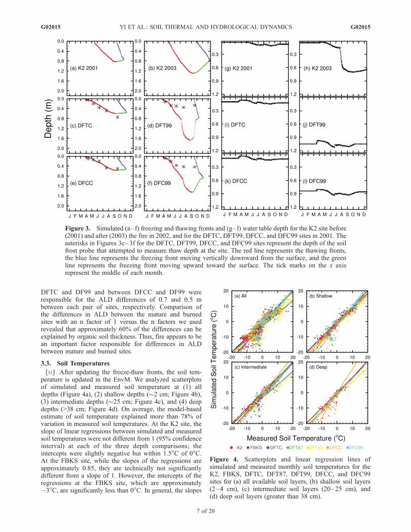
[28] In the EnvM, the freeze-thaw fronts were explicitlysimulated using the Stefan algorithm. At the K2 site, thesimulated prefire ALD reached 0.8 m in 2001 (Figure 3a).ALD measured at the nearby circumpolar active layermonitoring (CALM) network [Brown et al., 2000] sitewas 0.56 ± 0.14 cm in 2001. In 2002, half of the 14 cmorganic soil horizons at the K2 site was lost in the fire, andin 2003, the simulated ALD is more than 1.3 m. Both thereduction of organic soil horizons and warmer summer airtemperature at the K2 site (Figure 1a) contributed to thedeeper ALD in 2003.[29] The simulated maximum ALDs of DFTC and

DFT99 in 2001 were around 0.65 and 1.8 m, respectively(Figures 3c and 3d). Similarly, the simulated maximumALD at the DFCC and DFC99 sites are about 0.6 m and1.4 m, respectively (Figures 3e and 3f). The simulated andseasonal ALDs agree well at DFTC and DFCC in allmonths except September (Figures 3c and 3e) The ALD inSeptember is underestimated at DFTC and overestimated atDFCC, however, the simulation is within 1 standard devi-ation of measurement, 37 and 11 cm for DFTC and DFCC,respectively. At the recently burned sites, DFT99 andDFC99, the simulated thaw depth is similar to the observedthaw depth in April and May, but is deeper than observed inJune, July, and September (Figures 3d and 3f), The accuratemeasurement of thaw depth at these sites in July, August,and September was constrained by the existence of shallowgravel layer that prevented the permafrost probe frompenetrating deeper. Soil pits excavated shortly after the firein 1999 indicated that the permafrost table at DFT99 andDFC99 were deeper than 2 m and 1 m, respectively [Hardenet al., 2006].[30] Additional simulations were conducted for DFTC,

DFT99, DFCC, and DFC99 with the assumption that nfactor equals 1.00. The simulated ALDs are about 0.8, 1.5,0.8, and 1.3 m for DFTC, DFT99, DFCC, and DFC99,respectively. Differences in organic soil depths between

Figure 2. Scatterplots and linear regression lines ofsimulated and measured monthly evapotranspiration (ET)for the DFTC, DFT87, and DFT99 sites from 2002 to 2004.

1Auxiliary materials are available in the HTML. doi:10.1029/2008JG000841.


6 of 20

G02015

DFTC and DF99 and between DFCC and DF99 wereresponsible for the ALD differences of 0.7 and 0.5 mbetween each pair of sites, respectively. Comparison ofthe differences in ALD between the mature and burnedsites with an n factor of 1 versus the n factors we usedrevealed that approximately 60% of the differences can beexplained by organic soil thickness. Thus, fire appears to bean important factor responsible for differences in ALDbetween mature and burned sites.

3.3. Soil Temperatures

[31] After updating the freeze-thaw fronts, the soil tem-perature is updated in the EnvM. We analyzed scatterplotsof simulated and measured soil temperature at (1) alldepths (Figure 4a), (2) shallow depths (�2 cm; Figure 4b),(3) intermediate depths (�25 cm; Figure 4c), and (4) deepdepths (>38 cm; Figure 4d). On average, the model-basedestimate of soil temperature explained more than 78% ofvariation in measured soil temperatures. At the K2 site, theslope of linear regressions between simulated and measuredsoil temperatures were not different from 1 (95% confidenceinterval) at each of the three depth comparisons; theintercepts were slightly negative but within 1.5�C of 0�C.At the FBKS site, while the slopes of the regressions areapproximately 0.85, they are technically not significantlydifferent from a slope of 1. However, the intercepts of theregressions at the FBKS site, which are approximately�3�C, are significantly less than 0�C. In general, the slopes

Figure 3. Simulated (a–f) freezing and thawing fronts and (g–l) water table depth for the K2 site before(2001) and after (2003) the fire in 2002, and for the DFTC, DFT99, DFCC, and DFC99 sites in 2001. Theasterisks in Figures 3c–3f for the DFTC, DFT99, DFCC, and DFC99 sites represent the depth of the soilfrost probe that attempted to measure thaw depth at the site. The red line represents the thawing fronts,the blue line represents the freezing front moving vertically downward from the surface, and the greenline represents the freezing front moving upward toward the surface. The tick marks on the x axisrepresent the middle of each month.

Figure 4. Scatterplots and linear regression lines ofsimulated and measured monthly soil temperatures for theK2, FBKS, DFTC, DFT87, DFT99, DFCC, and DFC99sites for (a) all available soil layers, (b) shallow soil layers(2–4 cm), (c) intermediate soil layers (20–25 cm), and(d) deep soil layers (greater than 38 cm).


7 of 20

G02015

of the regressions for the Donnelly Flats sites are notsignificantly different from 1. However, the range of theintercepts at the Donnelly Flats sites is between �0.5�C and�3.5�C, with most of the intercepts significantly less than0�C. The negative intercepts are associated with under-estimates of soil temperature that largely occur duringwinter. See Table S2 in the auxiliary material for more detail.[32] The EnvM performed well in simulating soil tem-

perature at the K2 site before the fire event in 2002, butunderestimated the summer soil temperature (Figure 5a). Itis possible that fire alters the surface characteristics, and thatthe n factor following fire may be greater than 1. At theDonnelly Flats sites, the EnvM underestimated soil temper-atures during the winter of 2003–2004. The underestima-tion was about 6–10�C at the DFCC site (Figure 5b). Incomparison to other winters reported in Figure 5b, thewinter of 2003–2004 was characterized by substantiallylower precipitation and colder atmospheric temperature inour driving data sets (Figures 1c and 1f). The simulatedcolder soil temperatures in the winter 2003–2004 areconsistent with the climate data used to drive the simula-tions. In contrast, the measured soil temperature implies thatthe snowpack was thicker than in the other years, which isinconsistent with the precipitation in our driving data sets.Therefore, we suspect that the precipitation data are biasedin 2003–2004 or that wind redistribution of snow results insimilar snow depths at the sites in each year.

3.4. Water Table Depth

[33] As with the analysis of the simulated freeze-thawfronts, we analyzed the simulated WTDs for the K2 siteboth before (2001) and after (2003) the fire (Figures 3g and3h), and for the Donnelly Flats sites in 2001 (Figures 3i–3l). In the model simulation of the K2 site, the organic soilthickness was changed in August 2002. The WTDs at theK2 site increased to 70 cm in the following summer(Figure 3h), while those of 2001 are less than 10 cm. Theincrease of WTDs in 2003 is caused by the increase ofALDs, which are deeper than 1.3 m (Figure 3b). At theDonnelly Flats sites, the simulated WTDs decrease in Aprilbecause of snowmelt infiltration. During the growing sea-son, the simulated WTDs generally increase because ofevapotranspirational water losses, but there are occasionaldecreases in WTD because of rainfall events. In general, thesimulated WTDs of the mature forests (DFTC and DFCC)are shallower than those of the burned sites (DFC99 andDFT99) as deeper ALDs increase base flow at the burnedsites.

3.5. Soil Moisture

[34] The soil moisture of each soil layer in the EnvM isupdated immediately after soil temperature is updated. Weanalyzed scatterplots of simulated and measured soiltemperature at (1) all depths (Figure 6a), (2) shallowdepths (�2 cm; Figure 6b), (3) intermediate depths

Figure 5. Comparisons between simulated (crosses) and measured (circles) monthly soil temperaturesat different depths of the (a) K2 site from 1999 to 2006, at which fire occurred in 2002; and of the (b)DFCC site from 2001 to 2004.


8 of 20

G02015

(�25 cm; Figure 6c), and (4) deep depths (>38 cm;Figure 6d). In general, the correspondence between simu-lated and measured soil moisture is not as tight as thecomparison between simulated and measured soil tempera-ture. At the K2 site, the slope of linear regressions betweensimulated and measured soil moistures was significantlyless than 1, with the slope highest (0.84) for the intermediatedepth comparison, which was the only comparison in whichthe intercept was not significantly different from 0�C. At theFBKS site, the slopes of the regressions were not differentthan 1 and the intercepts were not significantly differentfrom 0�C. At Donnelly Flats sites, the slopes of theregressions were generally not significantly different from1 and the intercepts were generally not significantly differ-ent from 0�C. See Table S3 in the auxiliary material formore detail.[35] The most successful simulations at all sites where

those of the intermediate depths (�25 cm) (Figure 6c),which captured the seasonal variations (Figure 7). It isdifficult to determine if the mismatches at shallow depthsindicate problems with the model at shallow depths or areassociated with biases in the measurements as it is verydifficulty to accurately measure soil moisture in very porousorganic soils [Yoshikawa et al., 2004; Overduin et al.,2005]. We suspect that the mismatches in the deeper soil

layers are associated with uncertainties of representinglateral drainage in our simulations as the model assumesthat lateral drainage only occurs in mineral soils at depthsdeeper than 80 cm. For the only very poorly drained site,FBKS, the simulated soil moistures are saturated at inter-mediate depth (30 cm), which are overestimated comparedwith observations (Figure 7). Several additional simulationswere conducted for FBKS in which several parameters anddriving variables were varied, but the results were notimproved. The assumption of no lateral drainage in theorganic soil horizons appears to not be valid for this site,which usually has ALD occurring in organic soil horizons.For moderately well drained sites, at intermediate depths,there are two notable types of differences between simulatedand measured soil moisture. One is an artifact associatedwith the thermal timing of phase change in which thesimulated increase in soil moisture lags the measuredincrease in soil moisture because the model assumes 5%volumetric unfrozen water content when soil is frozen, e.g.,in the springs 2001 and 2002 at the DFTC site (Figure 7).The other difference is associated with improper represen-tation of soil texture in the model, e.g., the porosity of themineral soil at 25 cm of the DFTC site is specified to be lessthan 50%, but the measured volumetric water content forthis site exceeded 60% in summer 2002.

Figure 6. Scatterplots and linear regression lines of simulated and measured monthly soil moisture(volumetric water content, %) for the K2, FBKS, DFTC, DFT87, DFT99, DFCC, and DFC99 sites at (a)all available soil layers (all), (b) shallow layers (2–4 cm), (c) intermediate soil layers (20–25 cm), and (d)deep soil layers (greater than 38 cm).


9 of 20

G02015

3.6. Sensitivity Analysis

[36] The ALD and WTD of the baseline simulation of thesensitivity analysis are 120 and 74 cm for the moderatelywell drained black spruce forest, respectively, and are 63and 13 cm for the poorly drained black spruce forest. Thesensitivity indices of ALD and WTD for the differentsimulations of the sensitivity analysis are plotted againsteach other in Figures 8a and 8b for the moderately welldrained and poorly drained black spruce forests. The sen-sitivity of the ALD or WTD responses is represented by thedistance of each point in Figures 8a and 8b from the origin;larger distances indicate greater sensitivity.[37] Warm season air temperature (Ta), organic soil

thickness (OS), and minimum soil thermal conductivity(TcSlMin) directly affect the thermal regime of soil(Figure 9). An increase of Ta or TcSlMin or a decrease ofOS caused an increase of ALD and vice versa (Figures 8aand 8b). Increases of ALD cause increases of WTD for

moderately well drained black spruce forest, due to theincreases of base flow/drainage. But the change of WTD forpoorly drained black spruce forest is small, since the baseflow is set to 0. These differences are demonstrated inFigures 8a and 8b; the symbols in Figure 8b are moreclustered near the vertical axis than those in Figure 8a.[38] The role of subsurface drainage is also seen in

contrasting responses of WTD to decreases in rain in whichWTD of the poorly drained black spruce forest increases(see Figure 8b, region II), but WTD of the moderately welldrained forest increases (see Figure 8a, region III). Thedecreased soil moisture associated with rain initiallydecreases the thermal conductivity of the soil, which causesa decrease in ALD (see both Figures 8a and 8b). In themoderately well drained forest the decrease in ALD resultsin less subsurface drainage (Figure 9), which decreasesWTD. Because drainage is not affected by ALD in thepoorly drained forest, the decrease in rain increases WTD.

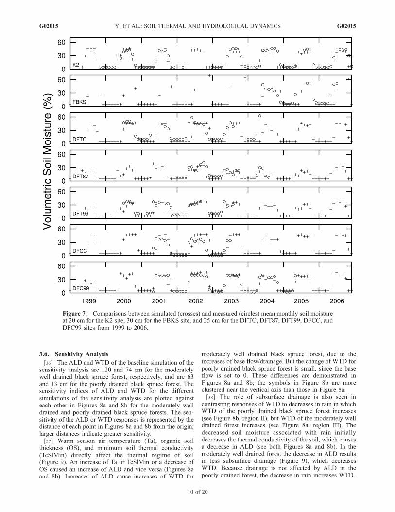
Figure 7. Comparisons between simulated (crosses) and measured (circles) mean monthly soil moistureat 20 cm for the K2 site, 30 cm for the FBKS site, and 25 cm for the DFTC, DFT87, DFT99, DFCC, andDFC99 sites from 1999 to 2006.


10 of 20

G02015

Figure 8. Sensitivity analysis results for a black spruce forest on (a) a moderately well drained soil and(b) a poorly drained soil. The factors to which active layer depth (ALD) and water table depth (WTD) aremost sensitive are farthest from the zero-zero point. Plus and minus markers within the parametersymbols represent increases and decreases of the factor, respectively. Ta, summer atmospherictemperature; OS, organic soil thickness; LAI, leaf area index; Fsat, topography factor; DrainMax,maximum drainage rate; TcSlMin, minimum soil thermal conductivity; RhoSnMax, maximum snowdensity; AlbSn, snow albedo; EvSlMin, minimum soil evaporation fraction.

Figure 9. Relationships among the parameters/variables evaluated in the sensitivity analysis(diamonds), processes (ellipses), and states (rectangles). Evaporation, soil surface evaporation;sublimation, snowpack sublimation; Ts deep, deep soil temperatures; TC shallow, shallow soil thermalconductivity; other notation is the same as that used in Figure 8. The circled pluses (or minuses) meanthat an increase of a parameter/variable at the beginning of the arrow will cause an increase (or adecrease) in the parameter/variable at the end of the arrow. Diamonds with dashed lines represent factorsthat directly affect water table depth (WTD); diamonds with solid lines represent factors directly affectingactive layer depth (ALD). The remaining parameters/variables are included in diamonds with dottedlines. For clarity, the effects of ALD on transpiration are not shown here.


11 of 20

G02015

[39] The estimates of ALD and WTD simulated by themodel were not responsive to changes in the other drivingvariables and parameters considered in the sensitivity anal-ysis. One would expect that soil moisture would be affectedby the surface evaporation ratio parameter (EvSlMin) andthe topography parameter (Fsat). This insensitivity is causedby short-term self-adjustment of model, i.e., if infiltration isreduced by a decrease in EvSlMin, then the surface soil willbecome drier and there will be less runoff and moreinfiltration with the next rain event (Figure 9). Other factorswe considered in the sensitivity analysis (radiation, LAI,and maximum snow albedo, AlbSnMax) have complexeffects on the dynamics of the EnvM and involve negativefeedback loops that result in low sensitivity of ALD andWTD (Figure 9). For example, as LAI increases ET willincrease, which will tend to result in a drier soil. However,when the soil is drier, the surface infiltration becomesgreater, which tends to result in a wetter soil. These negativefeedbacks limit the effect of increasing LAI on WTD.Thus, while the model does not demonstrate substantialsensitivity to radiation, LAI, and maximum snow albedo,and AlbSnMax, these factors are still quite important in soilthermal and hydrological dynamics of the EnvM.

4. Discussion

[40] With respect to evaluating model performance insimulating responses to fire, the tundra (K2) site providedboth preburn and postburn measurements to evaluate modelperformance. In contrast, the black spruce chronosequencesrepresent space-for-time substitutions. While space-for-timesubstitutions have been a powerful means for studyingprogressive changes in ecosystems after a major disturbance[Rastetter, 1996], it is important to recognize that differ-ences between sites of a chronosequence, for exampledifferences in mineral soil chemistry and disturbance history,may result in comparisons that are not completelyhomologous with sites that have predisturbance and post-disturbance measurements. This aspect of space-for-timesubstitutions complicates model-data comparisons in whichit is difficult to attribute whether model-data mismatches areassociated with model performance issues or data qualityissues. Even with these limitations to model-data compar-ison, the EnvM demonstrates substantial ability in simulat-ing the dynamics of evapotranspiration, soil temperature,active layer depth, soil moisture, and water table depth inresponse to both climate variability and fire disturbance.The model is capable of simulating changes in active layerdepth that affect water table depth through changes ofsubsurface drainage, changes that have the potential toinfluence biogeochemical dynamics. Our analyses alsoidentified several differences between model simulationsand field measurements that warrant attention. Below wediscuss what we have learned from evaluation of the EnvMwith respect to issues involving (1) atmospheric drivingvariables and (2) model parameters. We also briefly discussthe issue of soil moisture measurements in organic soils.

4.1. Issues Involving Atmospheric Driving Variables

[41] In our simulations, we used the estimates of daily airtemperature and n factor to estimate ground surface tem-perature for purposes of estimating heat transferred between

the ground and the atmosphere. The n factor, which is theratio of temperature at the soil surface to that in the air, isused by some studies to estimate ground surface tempera-ture from air temperature [Klene et al., 2001; Karunaratneand Burn, 2004]. However, the n factor is affected byground thermal properties and subsurface conditions[Karunaratne and Burn, 2004], and by vegetation cover[Klene et al., 2001]. The n factor values reported in theliterature range from 0.63 to 1.25 [Klene et al., 2001]. Mostecosystem models do not use the n factor approach toestimate ground surface temperature and assume thatground surface temperature is the same as air temperaturethat is generally measured at 2 m height. We have used the nfactor derived from the measurements at the sites analyzedin this study. Among the Donnelly Flats sites, the n factor ismuch greater at the recently burned sites than at the maturesites. At the K2 site, we assumed that the n factor of theburned site was equal to 1.00, which might represent anunderestimate that could be responsible for the underesti-mation of summer soil temperatures following fire in 2002.Land surface models calculate ground surface temperaturesthrough calculating ground surface energy balance based onsubhour resolution of atmospheric driving data, (e.g., CLM3[Oleson et al., 2004]). Because ecosystem models generallyuse daily or monthly resolution atmospheric driving data,they cannot adequately make use of the methodology usedin land surface models to calculate ground surface temper-ature. Given the sensitivity of ALD to air temperatureidentified in this study, some attention should be given toestimating more realistic ground surface temperature.[42] The accuracy of precipitation data sets has been an

important concern for applications of large-scale hydrolog-ical and ecosystem models in northern high-latitude regions[McGuire et al., 2008] because of the low density ofobservations and numerous issues involved in accuratelymeasuring snow fall [Yang et al., 2005]. We believe thatbiases in precipitation or issues of redistribution of snow areresponsible for some of the differences between simulatedand measured soil temperature, e.g., the snow fall at thebeginning of 2004 at Delta Junction is lower than snow fallat the beginning of the other years of our simulations.

4.2. Issues Involving Model Parameters

[43] The factors analyzed in the study can be broadlydivided into three categories: (1) factors that directly affectALD; (2) factors that directly affect WTD; and (3) factorsthat indirectly affect ALD and WTD through effects onvarious processes (Figure 9). Factors that directly affectALD included warm season air temperature, minimum soilthermal conductivity, and organic soil thickness. An impor-tant dynamic identified in our analysis of the model simu-lations is that changes in ALD often affect WTD throughchanges of subsurface drainage. However, the strength ofthis effect depends on whether a site is well or poorlydrained.[44] In the sensitivity analysis we conducted, we did not

evaluate all of the parameters in the model that affecthydrology. The parameters defining the hydraulic propertiesof moss, organic soil, and mineral soil can substantiallyaffect the hydrological dynamics of the model. With respectto moss, there are two main types of bryophyte groups inboreal black spruce forests, feathermoss (e.g., Hylocomium


12 of 20

G02015

splendens), which generally occurs in well to intermediatelydrained conditions, and Sphagnum, which generally occursin more poorly drained conditions [Manies et al., 2006].These moss types have distinct thermal, hydrological, andecophysiological characteristics [e.g., see Bisbee et al.,2001]. Feathermoss depends heavily on the precipitationand dew formation for water, while Sphagnum can wickwater from deeper soil through capillary action. The soilmoisture measurement at the FBKS site used in this studyprovides two data sets, one for soil pits with feathermosscover, and the other with Sphagnum [Kim et al., 2007]. Thesoil moisture at 30 cm of a ‘‘Sphagnum soil’’ is alwaysgreater than that of a ‘‘feathermoss soil.’’ In this study wedid not implement the different hydrologic properties ofthese different types of moss. It will be important toconsider the distinct hydrological and thermal propertiesof different types of moss that occur in moderately welldrained and poorly drained situations in future applicationsof the model.[45] There are significant differences in hydraulic prop-

erties among different types of organic soil [Letts et al.,2000]. Beringer et al. [2001] did not implement differencesamong different organic soils. We therefore defined poros-ities for moss, fibrous organic soil, and amorphous organicsoil based on field measurements for black spruce forests inManitoba, Canada [Yi et al., 2009]. In addition to porosity,pore size distribution is another important factor affectingwater movement in organic soils [Clapp and Hornberger,1978; Cosby et al., 1984]. If the same saturated hydraulicconductivity and pore size distribution are used for fibrousand amorphous organic soil, the fibrous organic soil withlarger porosity would tend to suck water from the amor-phous organic soil horizons below. However, amorphousorganic soil usually has much larger values of the pore sizedistribution parameter than fibrous organic soil, whichmeans that amorphous organic soil can hold water moretightly than fibrous organic soil. In this study, a larger valueof pore size distribution (i.e., 6) has been used for theamorphous organic horizon than for fibrous organic horizon(4 based on Beringer et al. [2001]). The proper parameter-ization of different types of organic soil continues to be akey challenge in the simulation of soil water dynamics.

4.3. Issues of Soil Moisture Measurement

[46] A key challenge in evaluating the simulation of soilmoisture is confidence in the accuracy and precision of themeasurements of soil moisture. We found that the EnvM isbetter in simulating soil moisture at depth than in simulatingsoil moisture near the surface. It is currently very challengingto measure soil moisture in surface organic soils because thehigh porosity creates substantial difficulties in calibratinginstruments used to measure soil moisture [Yoshikawa et al.,2004; Overduin et al., 2005]. The potential for substantialmeasurement error in field-based soil moisture estimatesmakesit difficult to ascertain what discrepancies between model- andfield-based estimates require attention in the model.

5. Conclusion

[47] This paper presented and evaluated a stable andefficient scheme for incorporating the interactions of soilthermal and hydrological processes in a terrestrial ecosys-

tem modeling framework. Our analysis using this frame-work revealed that changes in active layer depth often affectwater table depth through changes of subsurface drainage.Because these changes have the potential to influencebiogeochemical dynamics, we suggest that it is importantfor models of carbon dynamics in cold regions to morecomprehensively represent interactions between soil ther-mal and hydrological processes.[48] Key challenges identified in this study for evaluating/

improving model performance include (1) proper represen-tation of discrepancies between air temperature and groundsurface temperature; (2) minimization of precipitation biasesin the driving data sets; (3) improvement of the measure-ment accuracy of soil moisture in surface organic horizons;and (4) proper specification of organic horizon depth,hydrological properties, and soil thermal conductivity. Res-olution of these observational issues will help in reducingmodel uncertainties. As changes in organic horizons causedby wildfire have substantial effects on soil thermal andhydrological regimes, an important next step is to investi-gate how the dynamics of organic soil thickness associatedwith wildfire disturbance and ecological succession affectthe dynamics of permafrost and soil carbon in high latitudes.

Appendix A

[49] This part contains the detailed descriptions of thewater and energy fluxes among the atmosphere, canopy,snow and soil, and within soil layers. In the environmentalmodule (EnvM; Figure S1 in the auxiliary material), theground layers include snow layers, soil layers, and rocklayers. The soil layers include live moss, fibrous organicsoil, amorphous organic soil, and mineral soil. Elevenmineral soil types have been considered in this studyfollowing Beringer et al. [2001]. The parameters of theEnvM are provided in Table A1.

A1. Estimation of Daily Atmosphere DrivingVariables

A1.1. Incident Radiation

[50] The monthly short-wave irradiance incident on landsurface (NIRR) is provided as input (Wm�2). Daily radiation isestimated from monthly values through linear interpolation.

A1.2. Air Temperature

[51] The daily air temperature (Ta) is derived frommonthly values using linear interpolation.

A1.3. Precipitation

[52] The daily precipitation (mm/day) is downscaled frommonthly precipitation (mm/month) based on the algorithmof Liu [1996], as used by Zhuang et al. [2004]. The dailyprecipitation is identified as rain when the daily air temper-ature greater than 0�C, otherwise it is identified as snow.

Appendix B: Effects of Vegetation on Radiationand Water Fluxes

B1. Radiation

[53] NIRR is divided into three components: reflectanceback to the atmosphere, radiation intercepted by the canopy,


13 of 20

G02015

Table

A1.Param

etersUsedin

theEnvironmentalModule

ofTEM

a

Nam

eSymbol

Unit

Value

Sources

andComments

ParametersThatDoNotDependonVegetationorDrainage

Vegetation

VPD

Start

VPDstart

Pa

930

Startofconductance

reductionwhen

vaporpressure

deficitis

lower

than

thisvalue;

Whiteet

al.[2000]

VPD

Close

VPDclose

Pa

4100

Stomataareclosedwhen

vaporpressure

deficitislower

than

thisvalue;

Whiteet

al.[2000]

PPFD50

PPFD50

mmol�

m�2�

s�1

75

Theradiationat

whichthestomataare

50%

open;Whiteet

al.

[2000];usedin

Appendix

BSnow

Maxim

um

Albedo

asn,m

ax

-0.8

Roeshet

al.[2001];usedin

Appendix

CMinim

um

Albedo

asn,m

in-

0.4

Roeshet

al.[2001];usedin

Appendix

CSnow

density

of

freshly

fallen

snow

r sn,new

kgm

�3

120

Verseghy[1991];usedin

Appendix

E

Soil

Minim

um

thermal

conductivity

k sl,min

W�

m�1�

K�1

0.1

Hinzm

anet

al.[1991];usedin

Appendix

E

Minim

um

evaporation

ratio

Evr,min

-0.15

See

Appendix

D

Wiltingpoint

potential

Ymax

mm

�1.5

�105

Olesonet

al.[2004];used

inAppendix

BRock

Thermal

conductivity

k rW

�m

�1�

K�1

2ClauserandHuenges

[1995];usedin

Appendix

E

Nam

eSymbol

Unit

Dry

Wet

Sources

andComments

ParametersThatDependonDrainage

Soil

Maxim

um

drainagerate

Drainmax

mm

�s�

10.04

0See

Appendix

DTopographyparam

eter

Fsat

-0.3

0.3

See

Appendix

D

Nam

eSymbol

Unit

TUN

DEC

CON

Sources

andComments

ParametersThatDependonVegetation

Vegetation

Albedo

av

-0.19

0.19

0.1

Beringer

etal.[2005];

usedin

Appendix

BBoundarylayer

conductance

gbl

mm

�s�

10.04

0.01

0.08

Theparam

eter

fortundra

isdefined

based

onthe

C3grass

param

eter

of

Whiteet

al.[2000]

Cuticularconductance

gc

mm

�s�

10.00001

0.00001

0.00001

Whiteet

al.[2000]

Maxim

um

stomatal

conductance

gs,max

mm

�s�

10.005

0.005

0.003

Whiteet

al.[2000]

Snow

Maxim

um

snow

density

r sn,m

ax

kgm

�3

362

250

250

Based

onLingandZhang

[2006]andPomeroyet

al.

[1998];usedin

Appendix

E

aTUN,tundra;DEC,boreal

deciduousforest;CON,boreal

conifer

forest;Dry,moderatelywelldrained

soil;Wet,poorlydrained

soil.


14 of 20

G02015

and radiation that is passed through the canopy andbecomes incident on the ground surface.

B1.1. Radiation Reflectance to the Atmosphere (Rv2a)

[54]

Rv2a ¼ NIRR � av

where av is vegetation albedo. The albedos of tundra,deciduous, and conifer forest were assigned to be 0.19,0.19, and 0.10, respectively [Beringer et al., 2005].

B1.2. Radiation Through Canopy to theGround (Rv2g)

[55] Beer’s law is used to calculate the extinction ofradiation in canopy:

Rv2g ¼ NIRR� Rv2að Þe�ERLAI

where ER ( = 0.5) is a dimensionless extinction coefficientof radiation in the canopy. LAI is projected leaf area index.

B1.3. Radiation Intercepted by the Canopy (Rv)

[56]

Rv ¼ NIRR� Rv2a � Rv2g

B2. Water

B2.1. Water Intercepted by the Canopy

[57] The calculations of rain (Wv,r) and snow (Wv,s)interception by the canopy are the same as those describedin equations (A15) and (A16) of Zhuang et al. [2002].

B2.2. Water From the Canopy to the Atmosphere

[58] The overall water flux from the canopy to theatmosphere is calculated using the Penman-Monteithequation. The water flux consists of three components:(1) evaporation of canopy liquid water (Qv,evp), (2) subli-mation of canopy snow (Qv,sub), and (3) transpiration(Qv,trs). If there is intercepted rain or snow, the interceptedradiation (Rv) is first used to evaporate rain or sublimatesnow. The remaining energy is then used to drive thetranspiration formulation. The detailed equations for thesefluxes are described in Appendix D of Zhuang et al. [2004].Several modifications have been made for the calculation ofstomatal conductance:

gs ¼ gs;max f Tminð Þ f VPDð Þ f PPFDð Þ f Yð Þ

where gs and gs,max are the stomatal conductance andmaximum stomatal conductance (m � s�1), and f(Tmin),f(PPFD), and f(Y) are the effects of minimum airtemperature, radiation, and leaf water potential on stomatalconductance, respectively. The effect of f(PPFD), whichwas not considered by Zhuang et al. [2004], wasimplemented in the EnvM following Waring and Running[1998]:

f PPFDð Þ ¼ PPFD

PPFDþ PPFD50

where PPFD is the absorbed solar radiation by canopy (J �m2 � s�1), and PPFD50 is the value of PPFD at whichcaused f(PPFD) is 50% saturated. In this study, PPFD50 isset to 75 m mol � m�2 � s�1 or 16.5 J � m2 � s�1.[59] With the vertical distribution of soil water content

calculated, f(Y) is modified to include the effects of rootdistribution on transpiration, following Oleson et al. [2004]:

f Yð Þ ¼Xi

wiri 1� 10�10

where wi is plant wilting factor for layer i, and ri is fractionof roots in layer i. The plant wilting factor wi is calculatedas:

wi ¼Ymax � Yi

Ymax þ Ysat;iTi > 0

0 Ti < 0

8<:

where Ymax is a specified constant value for the wiltingpoint potential of leaves (�1.5 � 105 mm), Yi and Ysat,i aresoil water matric potential and saturated matric potential(mm) of layer i (see Appendix D), and Ti is the soiltemperature in layer i (�C).

B2.3. Water Fluxes From the Canopy to the Ground

[60] The water fluxes from the canopy to the groundconsist of four components including throughfall of snow orrain, and the ‘‘dripping’’ of snow or rain from the canopyafter throughfall. The throughfall fluxes of snow or rain arecalculated as the precipitation input of snow or rain minusthe interception of snow or rain. The ‘‘dripping’’ fluxes ofsnow or rain are calculated as the interception of snow orrain minus the sublimation or evaporation of snow or rain.

Appendix C: Effects of Snowpack on Radiationand Water Fluxes

[61] The snowpack is divided into a maximum of fivelayers, similar to the method used in CLM3 (CommunityLand Model, V3 [Oleson et al., 2004]). The snowpackaccumulates from the fluxes of snow throughfall and dripfrom the canopy, and it is subject to ablation from subli-mation and melt. The dynamics of the snow layers areimplemented using a double linked list structure, so thatwhen a snow layer is too thin it is combined with anadjacent snow layer or it is removed if there is no adjacentsnow layer. When a snow layer is too thick, it is divided intotwo snow layers. The criteria for the thickness range ofsnow layers are similar to those criteria used in CLM3.

C1. Radiation

[62] The radiation from the snowpack to the atmosphereis calculated as:

Rsn2a ¼ Rv2g � asn

where asn is snow albedo, which is calculated followingRoesh et al. [2001].

asn ¼ asn;max � asn;max � asn;min

� �Ta þ 10

10

asn,max = 0.8 and asn,min = 0.4 are maximum and minimumsnow albedo.


15 of 20

G02015

C2. Water

C2.1. Water From the Canopy to the Snowpack

[63] The throughfall and drip of snow from canopy areadded to snowpack.

C2.2. Water From the Snowpack to Atmosphere(Qsn2a)

[64] If air temperature is less than �1�C, then snowpackis sublimated using available radiation:

Qsn2a ¼ Rv2g � Rsn2a

� �SA= Lvap þ Lfus

� �

where SA = 0.6 is snow absorptivity [Zhuang et al., 2002],Lvap = 2.51 � 106 J � kg�1 is the latent heat of vaporization,and Lfus = 3.337 � 105 J � kg�1 is the latent heat of fusion.

C2.3. Water From Snowpack to the Soil

[65] If air temperature is greater than �1�C, snowpackcan be melted by radiation or by heat conduction. Theradiation-driven melt is calculated as:

Qsn2sl;rad ¼ Rv2g � Rsn2a

� �=Lfus

The heat conduction-driven melt is described below in E.

Appendix D: Effects of Soil on Radiationand Water Fluxes

D1. Radiation

[66] The radiation from soil surface to atmosphere iscalculated as:

Rsl2a ¼ Rv2g � asl

where asl is soil albedo, which is calculated following theNCAR LSM [Bonan, 1996] using color classes related tosoil types. The color class of moss is assigned to be 3following Beringer et al. [2001], and the color classes of thefibrous and amorphous organic layers are assigned to be 8,which can be exposed by fire, the darkest class. The overallreflectivity of soil is considered to be the average ofreflectivity of visible and near infrared radiation.

D2. Water

[67] The methods of the CLM3 are used to calculate thesurface runoff and base flow [Oleson et al., 2004]. Theinfiltration is estimated as the difference between input, i.e.,rain and/or snowmelt, and runoff. If the topsoil layers (morethan 2) are unfrozen, the finite difference equations are usedto solve for the movement of water between layers, with theinfiltration as top boundary condition, and zero drainage asthe bottom boundary condition.

D2.1. Surface Runoff (Qover) and Infiltration (Qinf l)

[68] Surface runoff (Qover, mm � s�1) is calculated fol-lowing method of CLM3 [Oleson et al., 2004]. The rest ofinput of water is considered as infiltration. Surface runoff iscalculated based on the water table depth and fraction ofsaturation, which is determined by a topography parameter,

Fsat. In this study, the default value from CLM3, 0.3, isused.

D2.2. Transpirational Loss of Soil Water

[69] On the basis of the fine root production fraction oversoil profile, each soil layer loses soil water through transpi-ration. The sum of soil water lost to transpiration is equal tothe transpirational flux calculated for the canopy (seeAppendix B).

D2.3. Evaporation (Qsl,evap) of Soil Water

[70] The calculation of potential evaporation (Qsl,pe) fromthe soil surface is same as that described in Appendix A ofZhuang et al. [2002], which is based on the Penmanequation. If the rain and snowmelt are greater than Qsl,pe,the actual evaporation is calculated as:

Qsl;evap ¼ 0:6� Qsl;pe

If rain and snowmelt are less than Qsl,pe,

Qsl;evap ¼ Evr � Qsl;pe

where Evr is defined as Evr =0:3DSR2, and DSR is the number of

days since the last rain. However, experiments have shownthat the evaporation from the soil surface is generallyunderestimated when downscaling precipitation frommonthly values to daily values. Therefore, in this study aminimum evaporation ratio (0.08) is assigned, based on theobserved water fluxes from DFT99 site, which was burnedin 1999.

D2.4. Water Movement Between Soil Layers

[71] On the basis of the calculations of evaporation,infiltration, and transpiration, the movement of soil waterbetween soil layers is calculated by solving Richards’equation. Because there are cases for which the updatedsoil water content of a soil layer can become negative ormore than porosity at a daily time step, an iterative methodis used to solve Richards’ equation. The initial time step atbeginning of each day is a half day. If after a time step anysoil water content is not reasonable (negative or greater thanporosity), then the time step is halved, and this continuesuntil the solution is reasonable. The solution continues untila 1-day period is fully covered.[72] The soil matric potential (y) and hydraulic conduc-

tivity (K) are calculated following Clapp and Hornberger[1978] and Cosby et al. [1984].

y ¼ysat

qliqqsat

�b

Tsl > 0

103Lf

g

Tsl � Tf

TslTsl � 0

8>>><>>>:

where ysat is saturated matric potential (mm), b is the Clappand Hornberger [1978] constant, g is gravitational accel-eration (m � s�2), Tsl is soil temperature (K), and Tf isfreezing point of liquid water (K).

K ¼ Ksat

qliqqsat

2bþ3


16 of 20

G02015

where Ksat is saturated hydraulic conductivity (mm � s�1).ysat, Ksat, and b are specified for each type of soil followingBeringer et al. [2001].

D2.5. Base flow (Qbf)

[73] After the soil water contents of all layers are updated,the base flow is calculated following method of CLM3[Oleson et al., 2004]. Drainmax is an important parameterdetermining the maximum rate of drainage from unsaturatedfraction, in this study, the default value of 0.04 mm/s, isused. In the CLM3, only the deep soil, 6–10 layers, hasbase flow. In this study, if the mineral soil layers, deeperthan 80 cm, are unfrozen, then there can be base flow fromthese layers, otherwise the base flow is 0. For poorlydrained soils, the base flow is assumed to be 0.

D2.6. Water Table Depth

[74] The WTD (depth from ground surface to groundwa-ter surface, m) is calculated following the method of Olesonet al. [2004]:

WTD ¼ zh;n �Xni¼1

siDzi

where zh,n is the distance between soil surface and thebottom of soil layer n, si is soil wetness of soil layer n, andDzi is the thickness of soil layer n.

Appendix E: Soil Thermal Dynamics

[75] In previous versions of TEM, the Goodrich methodwas to solve for soil thermal dynamics [Zhuang et al.,2001]. The Goodrich method first updates the soil/snowtemperatures of layers above and below freezing/thawingfronts (FTFs), and assumes 0�C for layers between twoFTFs, and then determines the positions of FTFs usingupdated temperatures. However, sometimes the Goodrichmethod cannot provide a valid solution for the position ofFTFs, and thus the soil temperatures. This instability getworse when the soil thermal properties are coupled with soilwater content. In EnvM, a stable snow/soil thermal modelhas been developed that, uses the Two-Directional StefanAlgorithm (TDSA) [Woo et al., 2004]. The TDSA cansatisfactorily simulate the positions of FTFs in a landsurface model when proper surface forcing is provided [Yiet al., 2006].

E1. Soil Freezing and Thawing Fronts

[76] In EnvM, the positions of FTFs are first determinedat a daily time step using the TDSA. The TDSA firstprocesses layers from top to bottom, using ground surfacetemperature as the forcing for the surface layer, until all theenergy (degree days) is used up, or the front meet thebottom boundary of soil. The temperature at the bottom offirst rock layer is then used as the forcing for the bottomboundary to force the deepest FTF upward; betweenSeptember and April, the temperature at the bottom of lastmineral layer is used instead. A FTF separates a layer intohomogeneous frozen and unfrozen parts. The snow/soilcolumn can be treated as a set of homogeneous frozen and

unfrozen sublayers. Take a positive driving temperature insummer as an example. At the beginning of the TDSA:

ddleft ¼ T0d

where T0 is the ground surface temperature (�C), d is day,and ddleft is the available degree days for phase change(�C day).[77] If a layer is frozen, then phase change will happen in

this layer. TDSA calculates

ddneed;i ¼ qildi Rsum;i þRi

2

where ddneed,i is the degree day (�C day) needed tocompletely thaw layer i, qi is the volumetric water contentof layer i (m3/m3), l is latent heat of fusion (J/m3), di is thethickness of layer i (m), Ri is the thermal resistance of layeri (Ks/J), Rsum,i is the sum of thermal resistance above layeri (Ks/J). Ri is defined as

Ri ¼ di=kunf ;i

where kunf,i is the unfrozen thermal conductivity (W � m�1 �K�1) of layer i, which is calculated following the methodof Johansen [1975]:

kunf ;i ¼ ksat;i � kdry;i� �

Ke þ Kdry;i

where Ke is Kersten number, which is related to soil watercontent. The parameters ksat,i and kdry,i are saturated anddry thermal conductivities of a soil layer, which arespecified for each soil layer type.[78] If ddneed,i is less than ddleft, the frozen state is

changed to unfrozen, and a thawing front is moved to thetop of next layer, and ddleft is recalculated:

ddleft ¼ ddleft � ddneed;i

Rsum,i is then updated by adding the thermal resistivity of thecurrent layer to the old value of Rsum,i and the TDSA thenproceeds to the next layer if it is not rock.[79] If ddneed,i is greater than ddleft,

dpart ¼ �kunf ;iRsum;i þ

ffiffiffiffiffiffiffiffiffiffiffiffiffiffiffiffiffiffiffiffiffiffiffiffiffiffiffiffiffiffiffiffiffiffiffiffiffiffiffiffiffiffiffiffiffik2unf ;iR

2sum;i þ

2kfrz;iddleft

lqi

s

where dpart is partial depth that can be thawed, and kfrz,i isthe frozen thermal conductivity of layer i (J/Kms). Athawing front will be created at a depth dpart relative to thetop of layer i. ddleft is set to zero and the iteration stops.[80] If a layer is unfrozen, the ddleft is kept unchanged,

Rsum,i is updated and the TDSA then proceeds to the nextlayer if the layer is not rock. After the movement of thawingfront downward, the same procedure is used to adjust thedeepest front upward.

E2. Temperatures of All Layers

[81] After the positions of FTFs are determined, thetemperature of each layer will be updated. If there is nofront in whole ground column, the temperature of each layer


17 of 20

G02015

will be updated by solving finite difference equations of alllayers, with the derived ground surface temperature from airtemperature as the top boundary condition. Because the heatflux around 50–100 m can neglected for a time period ofcenturies [Nicolsky et al., 2007], we assumed a zero heatflux as the lower boundary condition. If there is one front inwhole ground column, the layers above and below the frontwill be updated separately by solving two different sets ofequations assuming no phase change. If there are two ormore fronts in the whole soil column, the temperatures oflayers above first front will be updated by solving the finitedifference equation of layers above first front, and a similarmethod will be used to update temperatures below the lastfront. For layers between first and last front, the temper-atures are assumed to be 0�C.[82] The Crank-Nicholson scheme is used to solve the

finite difference equations of ground temperatures. To keepthe calculation stable, an adaptive step-size integrationapproach is used. The initial time step is a half day. Afteradvancing one time step, if the change of a layer’s temper-ature is greater than a specified threshold (0.1�C in thisstudy), the time step will be halved. Iteration continues untilthe calculation covers a full day.

E2.1. Snow Thermal Conductivity

[83] Snow thermal conductivity ksn (W � m�1 � K�1)are calculated following Goodrich [1982]:

ksn ¼ 2:9� 10�6r2sn

where rsn is the snow density in unit of kg � m�3, and thevalue of rsn ranges from new snow density rsn,new tomaximum snow density rsn,max following Verseghy [1991],with a time step of 1 day:

rsn ¼ rsn � rsn;max

� �e�t þ rsn;max

where t = 0.24 corresponds to an e-folding time of about4 days. rsn,new is specified to be 100 kg � m�3, whilersn,max is the maximum snow density, which is specified tobe 250 kg � m�3 for forest ecosystems [Pomeroy et al.,1998] and 362 kg � m�3 for tundra ecosystems [Ling andZhang, 2006].

E2.2. Soil Thermal Conductivity

[84] Soil thermal conductivity ksl (W � m�1 � K�1) iscalculated following Farouki [1986]:

ksl ¼Keksl;sat þ 1� Keð Þksl;dry Sr > 1� 10�7

ksl;dry Sr � 1� 10�7

�

where Ke is Kersten number, and Sr is soil wetness. Theparameters ksl,sat, which is the saturated thermal conductiv-ity, and ksl,dry, which is the dry thermal conductivity, arecalculated as:

ksl;sat ¼ k1�qsatsolid k

qliqliq k

qliceice ;

and

ksl;dry ¼ k1�qsatsolid kqsatair

where ksolid, kliq, kice, and kair are thermal conductivity ofsolid material, liquid, ice, and air, respectively. Theparameters qsat, qliq, and qice are porosity, volumetric liquidcontent, and volumetric ice content, respectively. Theparameters ksolid and qsat are specified for each type of soilfollowing Beringer et al. [2001]. In some cases, thesimulated ksl is too small for topsoil layers under very dryconditions. Therefore, the minimum thermal conductivityhas been set 0.1 W m�1 K�1 following Hinzman et al.[1991] to account for nonconductive heat exchange.

E2.3. Rock Thermal Conductivity

[85] The thermal conductivity of rock may vary by asmuch as a factor of two or three for the same type of rock.Because sedimentary rock underlies 72.9% of Alaska[Peucker-Ehrenbrink and Miller, 2003], we used a meanvalue of 2 W � m�1 � K�1, the thermal conductivity ofbedrock following Clauser and Huenges [1995].

E3. Volumetric Thermal Capacity

[86] The volumetric thermal capacity (J � m�3 � K�1) iscalculated based on the specific heat capacity (J� kg�1�K�1)and bulk density (kg � m�3). The specific heat capac-ities of soil are related to soil type, that of snow is2117.27 J � kg�1 � K�1, and that of rock is 1000 J �kg�1 � K�1. The bulk densities of soil are related to soiltype, the bulk density of snow is calculated during simula-tion, and the bulk density of rock is set to 2700 kg � m�3.

[87] Acknowledgments. We thank Dan Hayes of the Institute ofArctic Biology, who provided many of the driving data sets, and XingangFan, who provided station precipitation data that were corrected for bias.We also thank Eugenie Euskirchen, Qianlai Zhuang, two anonymousreviewers, and the associate editor for very thoughtful reviews of previousversions of this paper. This study was supported through grants provided aspart of the One Hundred People Plan of Chinese Academy of Sciences, theNorth American Carbon Program (NASA NNG05GD25G), the ArcticSystem Science Program (NSF OPP-0531047 and OPP-0327664) theBonanza Creek Long-term Ecological Program (funded jointly by NSFgrant DEB-0423442 and USDA Forest Service, Pacific Northwest ResearchStation grant PNW01-JV11261952-231), and the USGS Fate of Carbon inAlaskan Landscapes (FOCAL) Project.

ReferencesACIA (2004), Arctic Climate Impact Assessment, Cambridge Univ. Press,Cambridge, U. K.

Balshi, M. S., et al. (2007), Role of fire disturbance in the carbon dynamicsof the pan-boreal region: A process-based analysis, J. Geophys. Res., 112,G02029, doi:10.1029/2006JG000380.

Beringer, J., A. H. Lynch, F. Stuart Chapin III, M. Mack, and G. B. Bonan(2001), The representation of Arctic soils in the land surface model: Theimportance of mosses, J. Clim., 14, 3324–3335.

Beringer, J., S. F. Chapin, C. C. Thompson, and A. D. McGuire (2005),Surface energy exchanges along a tundra-forest transition and feedbacksto climate, Agric. For. Meteorol., 131, 143–161.

Bisbee, K. E., S. T. Gower, J. M. Norman, and E. V. Nordheim (2001),Environmental controls on ground cover species composition and pro-ductivity in a boreal black spruce forest, Oecologia, 129, 261–270.

Bonan, G. B. (1996), A land surface model (LSM Version 1.0) for ecolo-gical, hydrological, and atmospheric studies: Technical description andusers guide, NCAR Tech. Note Tn-417+STR, Natl. Cent. for Atmos. Res.,Univ. Corp. for Atmos. Res., Boulder, Colo.

Bond-Lamberty, B., C. Wang, and S. T. Gower (2005), Spatiotemporalmeasurement and modeling of stand-level boreal forest soil temperatures,Agric. For. Meteorol., 131, 27–40.

Bond-Lamberty, B., S. T. Gower, and D. E. Ahl (2007), Improved simula-tion of poorly drained forests using Biome-BGC, Tree Physiol., 27,703–715.

Brown, J., K. M. Hinkel, and F. E. Nelson (2000), The Circumpolar ActiveLayer Monitoring (CALM) Program: Research designs and Initial results,Polar Geogr., 24, 165–258.


18 of 20

G02015

Clapp, R. B., and M. G. Hornberger (1978), Empirical equations for somesoil hydraulic properties, Water Resour. Res., 14, 601–604.

Clauser, C., and E. Huenges (1995), Thermal conductivity of rocks andminerals, in Rocks Physics and Phase Relations: A Handbook of PhysicalConstants, AGU Ref. Shelf, vol. 3, edited by T. Ahrens, pp. 105–126,AGU, Washington, D. C.

Cosby, J. B., M. G. Hornberger, R. B. Clapp, and T. R. Ginn (1984), Astatistical exploration of the relationships of soil moisture characteristicsto the physical properties of soils, Water Resour. Res., 20, 682–690.

Davidson, E. A., and I. A. Janssens (2006), Temperature sensitivity of soilcarbon decomposition and feedbacks to climate change, Nature, 440,165–173.

Dunn, A. L., C. C. Barford, S. C. Wofsy, M. L. Goulden, and B. C. Daube(2007), A long-term record of carbon exchange in a boreal black spruceforest: Means, responses to interannual variability, and decadal trends,Global Change Biol., 13, 577–590.

Euskirchen, S. E., et al. (2006), Importance of recent shifts in soil thermaldynamics on growing season length, productivity, and carbon sequestra-tion in terrestrial high-latitude ecosystems, Global Change Biol., 12,731–750.

Farouki, O. T. (1986), Thermal properties of soils, Cold Reg. Res. and Eng.Lab., Hanover, N. H.

Friend, D. A., J. Schulz, and S. W. Running (1993), A physiology-basedgap model of forest dynamics, Ecology, 74, 792–797.

Goodrich, L. E. (1982), The influence of snow cover on the ground thermalregime, Can. Geotech. J., 19, 421–432.

Goulden, M. L., et al. (1998), Sensitivity of boreal forest carbon balance tosoil thaw, Science, 279, 214–216.

Harden, J., S. E. Trumbore, B. J. Stocks, A. I. Hirsch, S. T. Gower, K. P. O.Neill, and E. Kasischke (2000), The role of fire in the boreal carbonbudget, Global Change Biol., 6, suppl. 1, 174–184.

Harden, J., K. L. Manies, M. R. Turetsky, and J. C. Neff (2006), Effects ofwildfire and permafrost on soil organic matter and soil climate in interiorAlaska, Global Change Biol., 12, 2391–2403.

Hayes, D. J., A. D. McGuire, D. W. Kicklighter, T. J. Burnside, and J. M.Melillo (2009), The effects of land cover and land use change on thecontemporary carbon balance of the arctic and boreal ecosystems ofnorthern Eurasia, in Arctic Land Cover and Land Use in a ChangingClimate, edited by G. Gutman, chap. 5, Springer, New York, in press.

Hinzman, L. D., D. L. Kane, R. E. Gieck, and K. R. Everett (1991),Hydrologic and thermal properties of the active layer in the Alaskanarctic, Cold Reg. Sci. Technol., 19, 95–110.

Johansen, O. (1975), Thermal conductivity of soils, Ph.D. thesis, Univ. ofTrondheim, Trondheim, Norway.

Johnstone, J. F., and E. Kasischke (2005), Stand-level effects of soil burnseverity on postfire regeneration in a recently burned black spruce forest,Can. J. For. Res., 35, 2151–2163.

Ju, W., and J. Chen (2008), Simulating the effects of past changes inclimate, atmospheric composition, and fire disturbance on soil carbonin Canada’s forests and wetlands, Global Biogeochem. Cycles, 22,GB3010, doi:10.1029/2007GB002935.

Kanamitsu, M., et al. (2002), NCEP-DOE AMIP-II Reanalysis (R-2), Bull.Am. Meteorol. Soc., 83, 1631–1643.

Karunaratne, K. C., and C. R. Burn (2004), Relations between air andsurface temperature in discontinuous permafrost terrain near Nayo, YukonTerritory, Can. J. Earth Sci., 41, 1437–1451.

Kasischke, E., L. L. Bourgeau-Chavez, and J. F. Johnstone (2007),Assessing spatial and temporal variations in surface soil moisture infire-disturbed black spruce forests in Interior Alaska using spacebornesynthetic aperture radar imagery—Implications for postfire tree recruit-ment, Remote Sens. Environ., 108, 42–58.

Kim,Y.,M.Ueyama, F. Nakagawa, U. Tsunogai, Y. Harazono, andN. Tanaka(2007), Assessment of winter fluxes of CO2 and CH4 in boreal forest soilsof central Alaska estimated by the profile method and the chamber method:A diagnosis of methane emission and implications for the regional carbonbudget, Tellus, Ser. B, 59, 223–233.

Klene, A. E., F. E. Nelson, and N. I. Shiklomanov (2001), The n factor as atool in geocryological mapping: Seasonal thaw in the Kuparuk Riverbasin, Alaska, Phys. Geogr., 22, 449–466.

Letts, M. G., N. T. Roulet, N. T. Comer, M. R. Skarupa, and D. L. Verseghy(2000), Parametrization of peatland hydraulic properties for the CanadianLand Surface Scheme, Atmos. Ocean, 38, 141–160.

Liljedahl, A., L. D. Hinzman, R. Busey, and K. Yoshikawa (2007), Physicalshort-term changes after a tussock tundra fire, Seward Peninsula, Alaska,J. Geophys. Res., 112, F02S07, doi:10.1029/2006JF000554.

Ling, F., and T. Zhang (2006), Sensitivity of ground thermal regime andsurface energy fluxes to tundra snow density in northern Alaska, ColdReg. Sci. Technol., 44, 121–130.

Liu, H., and J. T. Randerson (2008), Interannual variability of surfaceenergy exchange depends on stand age in a boreal forest fire chronose-quence, J. Geophys. Res., 113, G01006, doi:10.1029/2007JG000483.

Liu, Y. (1996), Modeling the emissions of nitrous oxide (N2O) and methane(CH4) from the terrestrial biosphere to the atmosphere, Ph.D. thesis,219 pp., Mass. Inst. of Technol., Cambridge.

Manies, K., J. Harden, K. Yoshikawa, and J. Randerson (2001), The effectof soil drainage on fire and carbon cycling in central Alaska, U.S. Geol.Surv. Prof. Pap., 1678.

Manies, K. L., J. W. Harden, K. Yoshikawa, and J. Randerson (2003), Theimpact of soil drainage on fire and carbon cycling in central Alaska, inStudies by the U.S. Geological Survey in Alaska, edited by J. Galloway,U.S. Geol. Surv. Prof. Pap., 1678, 24 pp.

Manies, K., J. Harden, S. Silva, P. H. Briggs, and B. M. Schmid (2004),Soil data from Picea mariana stands near Delta Junction, Alaska of dif-ferent ages and soil drainage types, U.S. Geol. Surv. Open File Rep.,2004–1271, 19 pp.

Manies, K. L., J. W. Harden, and H. Veldhuis (2006), Soil data from amoderately well and somewhat poorly drained fire chronosequencenear Thompson, Manitoba, Canada, U.S. Geol. Surv. Open FileRep., 2006–1291, 13 pp.

McGuire, A. D., et al. (2008), The Western Arctic Linkage Experiment(WALE): Overview and synthesis, Earth Interact., 12, doi:10.1175/2008EI239.1.

Mitchell, T. D., and P. D. Jones (2005), An improved method of construct-ing a database of monthly climate observations and associated high-resolution grids, Int. J. Climatol., 25, 693–712.

Nicolsky, D. J., V. E. Romanovsky, V. A. Alexeev, and D. M. Lawrence(2007), Improvedmodeling of permafrost dynamics in aGCM land-surfacescheme, Geophys. Res. Lett., 34, L08501, doi:10.1029/2007GL029525.

Oelke, C., T. Zhang, and M. C. Serreze (2004), Modeling evidence forrecent warming of the Arctic soil thermal regime, Geophys. Res. Lett.,31, L07208, doi:10.1029/2003GL019300.

Oleson, K. W., et al. (2004), Technical description of the Community LandModel (CLM), NCAR Tech. Note TN-461+STR, Natl. Cent. for Atmos.Res., Univ. Corp. for Atmos. Res., Boulder, Colo.

Overduin, P. P., K. Yoshikawa, D. L. Kane, and J. Harden (2005), Compar-ing electronic probes for volumetric water content of low-density feath-ermoss, Sensor Rev., 25, 215–221.

Peucker-Ehrenbrink, B., and M. W. Miller (2003), Quantitative bedrockgeology of Alaska and Canada, Geochem. Geophys. Geosyst., 4(4), 8005,doi:10.1029/2002GC000449.

Pomeroy, J. W., M. D. Gray, R. K. Shook, B. Toth, R. Essery, A. Pietroniro,andN.Hedstrom (1998), An evaluation of snow accumulation and ablationprocesses for land surface modeling, Hydrol. Process., 12, 2339–2367.

Raich, J. W., E. B. Rastetter, J. Melillo, D. Kicklighter, P. A. Steudler, B. J.Peterson, A. L. Grace, B. Moore, and C. J. Vorosmarty (1991), Potentialnet primary productivity in South America: Application of a global model,Ecol. Appl., 1, 399–429.

Rastetter, E. B. (1996), Validating models of ecosystem response to globalchange, BioScience, 46, 190–198.

Robinson, C. H. (2002), Controls on decomposition and soil nitrogen avail-ability at high latitudes, Plant Soil, 242, 65–81.

Roesh, A., M. Wild, H. Gilgen, and A. Ohmura (2001), A new snow coverfraction parameterization for the ECHAM4GCM,Clim. Dyn., 17, 933–946.

Ruess, R. W., R. L. Hendrick, J. G. Vogel, and B. Sveinbjornsson (2006),The role of fine roots in the functioning of boreal forests, in Alaska’sChanging Boreal Forest, edited by F. S. Chapin III et al., pp. 189–210,Oxford Univ. Press, New York.

Shanley, J. B., and A. Chalmers (1999), The effect of frozen soil on snow-melt runoff at Sleepers River, Vermont, Hydrol. Process., 13, 1843–1857.

Sitch, S., et al. (2003), Evaluation of ecosystem dynamics, plant geographyand terrestrial carbon cycling in the LPJ dynamic global vegetation model,Global Change Biol., 9, 161–185.

Tarnocai, C. (2000), Carbon pools in soils of the Arctic, Subarctic andboreal regions of Canada, in Global Climate Change and Cold RegionsEcosystems, Adv. Soil Sci., edited by R. Lal, J. M. Kimble, and B. A.Stewart, pp. 91–103, Lewis, Boca Raton, Fla.

van Cleve, K., C. T. Dyrness, L. A. Viereck, J. F. Fox, F. S. Chapin III, andW. Oechel (1983), Taiga ecosystems in interior Alaska, BioScience, 33,39–44.

van Wijk, T. M., M. Williams, J. A. Laundre, and G. R. Shaver (2003),Interannual variability of plant phenology in tussock tundra: Modellinginteractions of plant productivity, plant phenology, snowmelt and soilthaw, Global Change Biol., 9, 743–758.

Verseghy, D. L. (1991), CLASS-A Canadian Land Surface Scheme forGCMs. I: Soil model, Int. J. Climatol., 11, 111–133.

Waring, R. H., and S. W. Running (1998), Forest Ecosystems: Analysis atMultiple Scales, Academic, San Diego, Calif.


19 of 20

G02015

White, M. A., P. Thornton, S. W. Running, and R. R. Nemani (2000),Parameterization and sensitivity analysis of the BIOM-BGC terrestrialecosystem model: Net primary production controls, Earth Interact., 4,1–85.

Wickland, K. P., and J. C. Neff (2007), Decomposition of soil organicmatter from boreal black spruce forest: Environmental and chemicalcontrols, Biogeochemistry, 87, 29–47, doi:10.1007/s10533-007-9166-3.

Wilson, K. B., et al. (2002), Energy balance closure at FLUXNET sites,Agric. For. Meteorol., 113, 223–243.

Woo, M.-K., A. M. Arain, M. Mollinga, and S. Yi (2004), A two-directionalfreeze and thaw algorithm for hydrologic and land surface modeling,Geophys. Res. Lett., 31, L12501, doi:10.1029/2004GL019475.

Yang, D., D. L. Kane, Z. Zhang, D. Legates, and B. Goodison (2005), Biascorrections of long-term (1973–2004) daily precipitation data over thenorthern regions, Geophys. Res. Lett., 32, L19501, doi:10.1029/2005GL024057.

Yi, S., A. M. Arain, and M.-K. Woo (2006), Modifications of a land surfacescheme for improved simulation of ground freeze-thaw in northern envir-onments, Geophys. Res. Lett., 33, L13501, doi:10.1029/2006GL026340.

Yi, S., M.-K. Woo, and A. M. Arain (2007), Impacts of peat and vegetationon permafrost degradation under climate warming, Geophys. Res. Lett.,34, L16504, doi:10.1029/2007GL030550.

Yi, S., K. Manies, J. Harden, and A. D. McGuire (2009), The characteristicsof organic soil in black spruce forests: Implications for the application ofland surface and ecosystem models in cold regions, Geophys. Res. Lett.,36, L05501, doi:10.1029/2008GL037014.

Yoshikawa, K., P. P. Overduin, and J. Harden (2004), Moisture contentmeasurement of moss (Sphagnum spp.) using commercial sensors,Hydrol.Process., 15, 309–318.

Zhang, Y., C. Li, C. C. Trettin, H. Li, and G. Sun (2002), An integratedmodel of soil, hydrology, and vegetation for carbon dynamics in wetlandecosystems, Global Biogeochem. Cycles, 16(4), 1061, doi:10.1029/2001GB001838.

Zhuang, Q., V. E. Romanovsky, and A. D. McGuire (2001), Incorporationof a permafrost model into a large-scale ecosystem model: Evaluation of

temporal and spatial scaling issues in simulating soil thermal dynamics,J. Geophys. Res., 106(D24), 33,649–33,670.

Zhuang, Q., A. D. McGuire, J. Harden, K. P. O’Neill, V. E. Romanovsky,and J. Yarie (2002), Modeling soil thermal and carbon dynamics of afire chronosequence in interior Alaska, J. Geophys. Res., 107, 8147,doi:10.1029/2001JD001244 [printed 108(D1), 2003].

Zhuang, Q., et al. (2003), Carbon cycling in extratropical terrestrial eco-systems of the Northern Hemisphere during the 20th century: A modelinganalysis of the influences of soil thermal dynamics, Tellus, Ser. B, 55,751–776.

Zhuang, Q., J. Melillo, D. Kicklighter, R. G. Prinn, A. D. McGuire, P. A.Steudler, B. S. Felzer, and S. Hu (2004), Methane fluxes between terres-trial ecosystems and the atmosphere at northern high latitudes duringthe past century: A retrospective analysis with a process-based biogeo-chemistry model, Global Biogeochem. Cycles, 18, GB3010, doi:10.1029/2004GB002239.

��J. Harden and K. Manies, U.S. Geological Survey, Menlo Park, CA

94025, USA.L. Hinzman, Y. Kim, and A. Liljedahl, International Arctic Research

Center, University of Alaska Fairbanks, Fairbanks, AK 99775, USA.E. Kasischke, Department of Geography, University of Maryland, 2181

LeFrak Hall, College Park, MD 20742, USA.H. Liu, Department of Physics, Atmospheric Sciences and General

Sciences, Jackson State University, Jackson, MS 39217, USA.S. Marchenko and V. Romanovsky, Geophysical Institute, University of

Alaska Fairbanks, Fairbanks, AK 99775, USA.A. D. McGuire, Alaska Cooperative Fish and Wildlife Research Unit,

U.S. Geological Survey, University of Alaska Fairbanks, Fairbanks, AK99775, USA.J. Randerson, Department of Earth System Science, University of

California, Irvine, CA 92697, USA.S. Yi, State Key Laboratory of Cryosphere Sciences, Cold and Arid

Regions Environmental and Engineering Institute, Chinese Academy ofSciences, Lanzhou, Gansu 730000, China. ([email protected])


20 of 20

G02015

interactions between soil thermal and hydrological … between soil thermal and hydrological...

Documents