Interaction of Electron and Photons with Matter

In addition to the references listed in the first lecture (of this part of the course)

see also “Calorimetry in High Energy Physics” by Richard Wigmans.

(Oxford University Press,2000)

This is actually an excellent book, which I would encourage you all to have a look at at some point.

I will show some plots from this in today’s lecture.

Bremsstrahlung

Lead (Z = 82)Positrons

Electrons

Ionization

Moller (e−)

Bhabha (e+)

Positron annihilation

1.0

0.5

0.20

0.15

0.10

0.05

(cm

2g−

1 )

E (MeV)10 10 100 1000

1 E−

dE dx

(X0−1

)Interactions of Electron and Photons with Matter

Photon Energy

1 Mb

1 kb

1 b

10 mb10 eV 1 keV 1 MeV 1 GeV 100 GeV

Lead (Z = 82)− experimental σtot

σp.e.

κe

Cros

ssec

tion

(bar

ns/a

tom

)

aσR y el igh

σCom t np o

κn cuelectron/positrons

photons

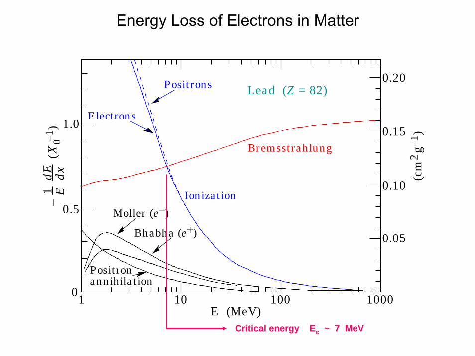
Critical energy Ec ~ 7 MeV

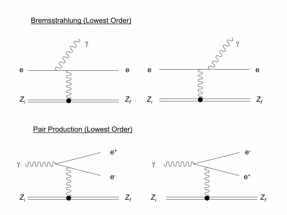
First important observation is that for energies above about 10 MeV (here in Pb) the energy loss mechanisms are in each case dominated by a single process, bremsstrahlung for the electrons (and positrons) and pair production for the photons.

Note also that these processes are related (so their amplitudes are related)

Zi Zf Zi Zf

e e e e

γ γ

Zi Zf Zi Zf

γ γ

e+ e-

e- e+

Bremsstrahlung (Lowest Order)

Pair Production (Lowest Order)

Bremsstrahlung

Lead (Z = 82)Positrons

Electrons

Ionization

Moller (e−)

Bhabha (e+)

Positron annihilation

1.0

0.5

0.20

0.15

0.10

0.05

(cm

2g−

1 )

E (MeV)10 10 100 1000

1 E−

dE dx

(X0−1

)

Energy Loss of Electrons in Matter

Critical energy Ec ~ 7 MeV

Electron/Positron Interactions with Matter

In general electrons and positrons lose energy in matter in almost identical ways. There are however some small differences:

In collisions with atomic electrons we have:

Møller scattering for electrons (two lowest-order diagrams in QED)

Bhabha scattering for positrons (two lowest-order diagrams in QED)

These contributions are sizeable only for low energies (below about 10 MeV) and are never dominant. Differences are visible in the plot on the previous slide (where annihilation component of Bhabha scattering is plotted separately).

Small difference in the ionization energy losses for electrons and positrons is also attributable to differences between the Møller and Bhabha scattering cross-sections

The size of the momentum transfer is what determines whether the interaction leads to ionization or just excitation.

Energy Loss of Electrons and Positrons

⎛ ⎞ ⎛ ⎞ ⎛ ⎞= +⎜ ⎟ ⎜ ⎟ ⎜ ⎟⎝ ⎠ ⎝ ⎠ ⎝ ⎠tot rad coll

dE dE dEdx dx dx

Collision losses similar to those for heavy charged particles with some differences:

For electrons need to account for indistinguishability of final state electrons in scattering processes

For positrons need to account for annihilation effects

Kinematics are different: maximum allowed energy transfer in a single collision is Te/2 where Te is the kinetic energy of the electron or positron.

Accounting for these effects one can obtain a version of the Bethe-Bloch equation for the dE/dx losses of electrons and positrons:

Total energy loss come from collisions and from radiation which dominates at high energies:

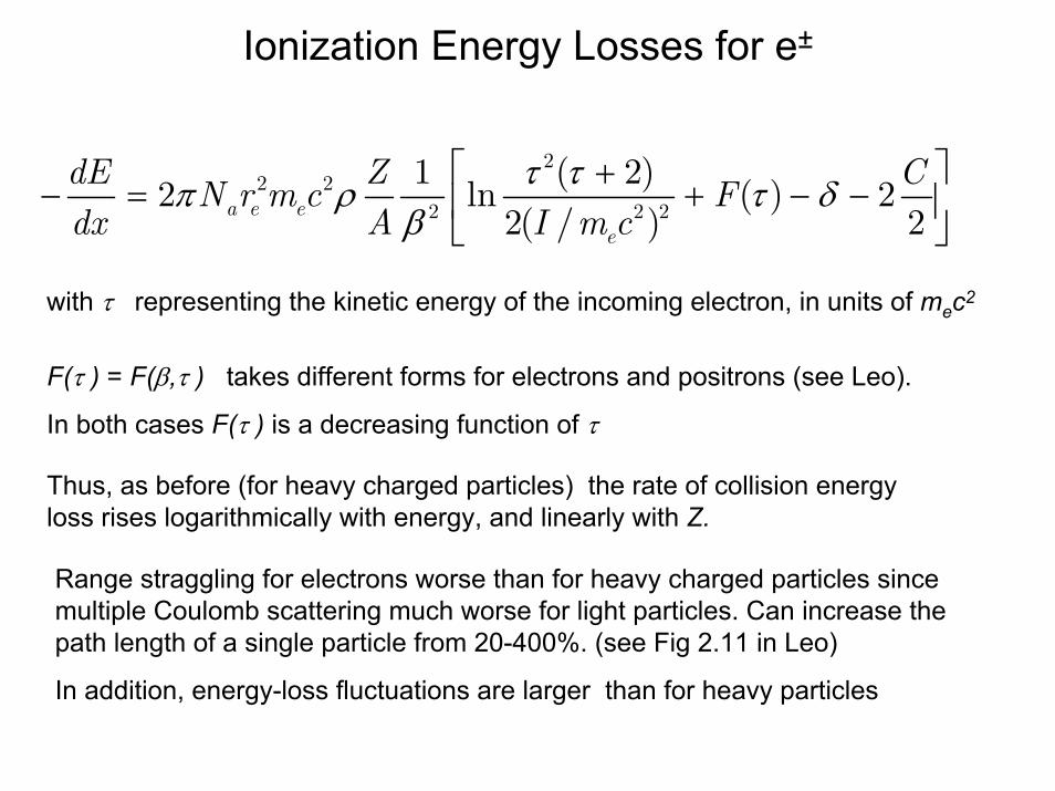
Ionization Energy Losses for e±

τ τπ ρ τ δβ

⎡ ⎤+− = + − −⎢ ⎥

⎣ ⎦

22 2

2 2 2

1 ( 2)2 ln ( ) 22( / ) 2a e e

e

dE Z CN r m c Fdx A I m c

with τ representing the kinetic energy of the incoming electron, in units of mec2

F(τ ) = F(β,τ ) takes different forms for electrons and positrons (see Leo).

In both cases F(τ ) is a decreasing function of τ

Thus, as before (for heavy charged particles) the rate of collision energy loss rises logarithmically with energy, and linearly with Z.

Range straggling for electrons worse than for heavy charged particles since multiple Coulomb scattering much worse for light particles. Can increase the path length of a single particle from 20-400%. (see Fig 2.11 in Leo)

In addition, energy-loss fluctuations are larger than for heavy particles

At energies below a few hundred GeV, only electrons and positrons lose significant amounts of energy through radiation.

Emission probability varies as m-2, so losses for electrons exceed those for muons by ( mµ / me )2 ~ 40000.

Bremsstrahlung depends on the strength of the electric field seen by the particle (usually the nuclear electric field) so screening due to atomic electrons needs to be accounted for.

Cross-section is therefore dependent not only on the electron energy, but also on the impact parameter and the Z of the material.

Effects of screening are parameterized in the following quantity:

Bremsstrahlung

νξ ν= = +2

1/3 00

100 em c h E E hE EZ

ξ = 0 represents complete screening; ξ 1 corresponds to no screening

Frequency of emitted γ

[Relevant at high energy]

For the limiting cases of no screening and complete screening the cross sections are

ν εσ α εν ν

⎡ ⎤⎛ ⎞= + − − −⎜ ⎟ ⎢ ⎥⎝ ⎠ ⎣ ⎦2 2 2 0

2

22 14 1 ln ( )3 2e

e

E Edd Z r f Zm c h

ν ε εσ α εν

−⎧ ⎫⎛ ⎞ ⎡ ⎤= + − − +⎨ ⎬⎜ ⎟ ⎣ ⎦⎝ ⎠⎩ ⎭2 2 2 1/324 1 ln(183 ) ( )

3 9edd Z r Z f Z

( ) ε−⎡ ⎤≅ + + − + − = =⎣ ⎦12 2 2 4 6

0( ) 1 0.20206 0.0369 0.0083 0.002 /137 /f Z a a a a a a Z E E

get energy loss due to radiation by integrating dσ over the allowable energy range

( )ν σν ν νν

⎛ ⎞− =⎜ ⎟⎝ ⎠ ∫ 0

00,

rad

dE dN h E ddx d

Where N is the number of atoms / cm3 (density of scattering centers) = Na ρ / A

and ν0 = E0 / h

ξ 1

ξ ~ 0

( )ν σν ν νν

⎛ ⎞− = Φ Φ =⎜ ⎟⎝ ⎠ ∫ 0

0 000

1with ,rad radrad

dE dNE h E ddx E d

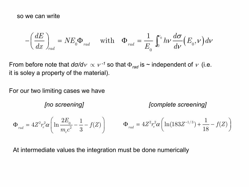
so we can write

From before note that dσ/dν ∝ ν -1 so that Φrad is ~ independent of ν (i.e. it is soley a property of the material).

α⎛ ⎞

Φ = − −⎜ ⎟⎝ ⎠

2 2 02

2 14 ln ( )3erad

e

EZ r f Z

m cα −⎛ ⎞Φ = + −⎜ ⎟⎝ ⎠

2 2 1/3 14 ln(183 ) ( )18erad Z r Z f Z

For our two limiting cases we have

[no screening] [complete screening]

At intermediate values the integration must be done numerically

Comparing the form of the radiation energy loss to that of the collisional energy loss we can make the following observations:

The ionization energy loss rises logarithmically with energy and linearly with Z

The bremsstrahlung energy loss rises ~ linearly with energy and quadratically with Z.

This explains the dominance of radiation energy loss at all but the lowest energies.

A further difference has to do with statistical fluctuations. Collisional energy loss is typically quasi-continuous, coming from a large number of small-energy-loss collisions.

In bremsstrahlung there is a high probability for almost all of the energy to be emitted in a small number (one or two) photons. The corresponding statistical fluctuations therefore have a larger effect.

Contribution from Atomic Electrons

There will of course also be a contribution to the radiation losses from interactions with the electromagnetic field of the atomic electrons. The calculation for these interaction is similar to that for the interaction with nuclei, and give a similar result except with the Z2 replaced by Z.

So to account for these interaction we can just replace Z2 with Z(Z+1) in all expressions.

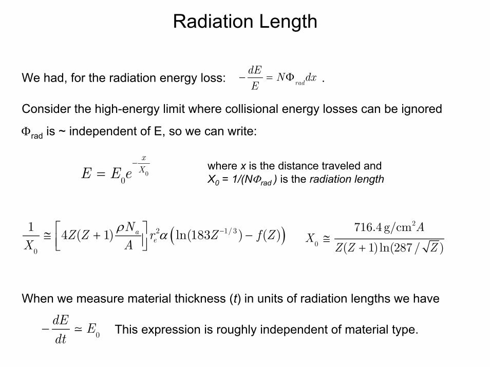
We had, for the radiation energy loss: .

Consider the high-energy limit where collisional energy losses can be ignored

Φrad is ~ independent of E, so we can write:

Radiation Length

− = ΦraddE N dxE

−= 0

0

xXE E e

( )ρ α −⎡ ⎤≅ + −⎢ ⎥⎣ ⎦2 1/3

0

1 4 ( 1) ln(183 ) ( )ae

NZ Z r Z f ZX A

where x is the distance traveled and X0 = 1/(NΦrad ) is the radiation length

≅+

2

0

716.4 g/cm

( 1)ln(287/ )

AX

Z Z Z

When we measure material thickness (t) in units of radiation lengths we have

− 0

dE Edt

This expression is roughly independent of material type.

Definition of Critical Energy

2 5 10 20 50 100 200

CopperX0 = 12.86 g cm−2

Ec = 19.63 MeV

dE

/dx

× X

0 (M

eV)

Electron energy (MeV)

10

20

30

50

70

100

200

40

Brems = ionization

Ionization

Rossi:Ionization per X0= electron energy

Total

Brem

s ≈ EExa

ctbr

emss

trah

lung

Mentioned the critical energy earlier. There are two definitions. One is the one we mentioned earlier. The other, due to Rossi, defines Ec as the energy at which the ionization energy loss per radiation length is equal to the electron energy.

The two are equivalent in the approximation that = 0/rad

dE E Xdx

Interactions of Photons with Matter

Photon Energy

1 Mb

1 kb

1 b

10 mb10 eV 1 keV 1 MeV 1 GeV 100 GeV

(b) Lead (Z = 82)- experimental σtot

σp.e.

κe

Cro

ss s

ectio

n (

barn

s/at

om)

Cro

ss s

ectio

n (

barn

s/at

om)

10 mb

1 b

1 kb

1 Mb

(a) Carbon (Z = 6)

σRayleigh

σg.d.r.

σCompton

σCompton

κnuc

κnuc

κe

σp.e.

- experimental σtotAs for electron / positron interactions, at all but the lowest energies, the interaction cross-section for photons is dominated by a single process (which is related to the bremsstrahlung energy loss process of e±)

Note that as soon as a photon has undergone such an interaction it is no longer a photon, but instead is an electron positron pair which will in turn lose energy via bremsstrahlung producing a photon which then pair produces etc……

Electromagnetic Showers

discuss this in a moment

Photon Interactions in Lead

Photon Energy

1 Mb

1 kb

1 b

10 mb10 eV 1 keV 1 MeV 1 GeV 100 GeV

(b) Lead (Z = 82)- experimental σtot

σp.e.

κe

Cro

ss s

ecti

on (

barn

s/at

om)

σg.d.r.

σCompton

κnuc

σp.e. = atomic photoelectric effect

σRaleigh = Raleigh (coherent) scattering

σCompton = Incoherent scattering

knuc = pair production in nuclear field

ke = pair production electron field

σg.d.r = Photonuclear interactions (nuclear breakup)

Cross-sections plotted, not energy loss

See also Fig. 2.7 in Wigmans

Attenuation Length

Photon energy

100

10

10–4

10–5

10–6

1

0.1

0.01

0.001

10 eV 100 eV 1 keV 10 keV 100 keV 1 MeV 10 MeV 100 MeV 1 GeV 10 GeV 100 GeV

Abs

orpt

ion

len

gth

λ (

g/cm

2)

Si

C

Fe Pb

H

Sn

For electrons and positrons we talk about the radiation length to quantify the expected energy loss over a certain distance in material.

For photons interaction via pair production, once the photon has interacted it is no longer a photon, so we talk in this case about the photon attenuation length.

We will see that this is given by

λ = 0

97X

Interactions of photons with matter

As we have seen previously, at very low energies the photoelectric effect dominates

Other processes at low energy:

Compton scattering γe γe well understood from QED. If photon energy is high wrtbinding energies then atomic electrons can be treated as unbound.

Rayleigh scattering: scattering of photons by the atoms as a whole. All electrons in the atom participate in a coherent manner. This is also called coherent scattering. There is no associated energy loss, only a change in the direction of the photon.

Photo-nuclear interactions causing nuclear breakup. Contribute mainly in a small energy regions around 10 MeV (in Pb) (most notable the Giant Dipole Resonance)

Pair Production γ e+ e-

Cannot happen in free space due to conservation of 4-momentum. Need to conserve 4-momentum through interaction with nuclear field. As was the case with bremsstrahlung, there is also a small contribution from interaction with the electric field of the atomic electrons (see plot. σ much smaller).

Photon must have an energy of at least 2mec2 = 1.022 MeV

As this process involves interactions with the nuclear field in much the same way as the bremsstrahlung process (remember, the processes are similar) the screening of the nuclear charge must again be accounted for. This time the (very similar) screening parameter is

γνξ −+

−+

= = +2

1/3

100 em c h E E EE E Z

Energy of electron

σ αν ν

− − −+ + ++

⎡ ⎤+ += − −⎢ ⎥

⎣ ⎦

2 22 2

3 2

2 /3 2 14 ln ( )( ) 2e

e

E E E E E Ed Z r dE f Z

h m c h

σ αν

−− −+ + +−+

⎧ ⎫⎛ ⎞ ⎡ ⎤= + + − +⎨ ⎬⎜ ⎟ ⎣ ⎦⎝ ⎠⎩ ⎭2 2 2 2 1/3

3

24 ln(183 ) ( )

( ) 3 9edE E E E E

d Z r E E Z f Zh

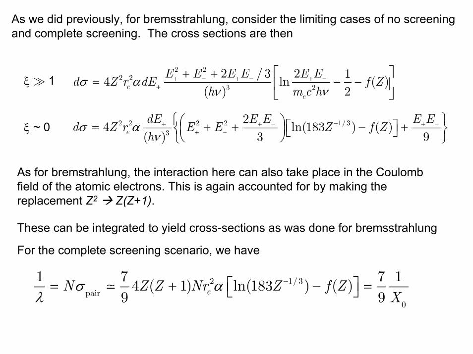
ξ 1

ξ ~ 0

As we did previously, for bremsstrahlung, consider the limiting cases of no screening and complete screening. The cross sections are then

As for bremstrahlung, the interaction here can also take place in the Coulomb field of the atomic electrons. This is again accounted for by making the replacement Z2 Z(Z+1).

These can be integrated to yield cross-sections as was done for bremsstrahlung

For the complete screening scenario, we have

σ αλ

−⎡ ⎤= + − =⎣ ⎦2 1/3

pair0

1 7 7 14 ( 1) ln(183 ) ( )9 9eN Z Z Nr Z f Z

X

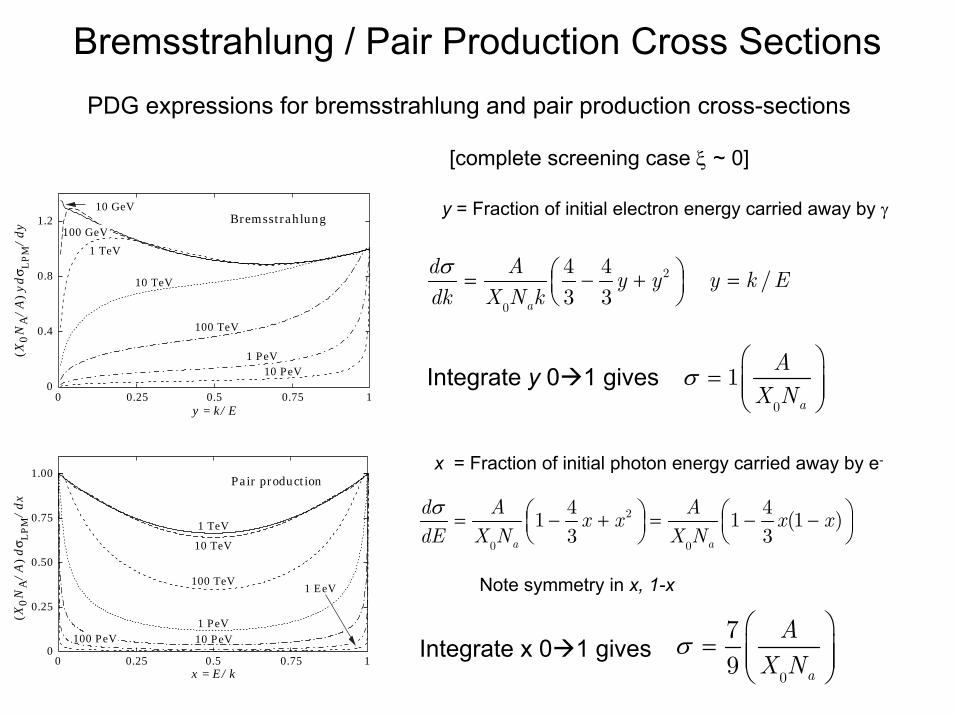
Bremsstrahlung / Pair Production Cross Sections

0 0.25 0.5 0.75 10

0.25

0.50

0.75

1.00

x = E/k

Pair production

(X0

NA

/A

) d

σ LP

M/

dx

1 TeV

10 TeV

100 TeV

1 PeV10 PeV

1 EeV

100 PeV

0

0.4

0.8

1.2

0 0.25 0.5 0.75 1y = k/E

Bremsstrahlung

(X0

NA

/A

) yd

σ LP

M/

dy

10 GeV

1 TeV

10 TeV

100 TeV

1 PeV10 PeV

100 GeV

σ ⎛ ⎞= − + =⎜ ⎟⎝ ⎠

2

0

4 4 /3 3a

d A y y y k Edk X N k

σ ⎛ ⎞ ⎛ ⎞= − + = − −⎜ ⎟ ⎜ ⎟⎝ ⎠ ⎝ ⎠

2

0 0

4 41 1 (1 )3 3a a

d A Ax x x xdE X N X N

y = Fraction of initial electron energy carried away by γ

x = Fraction of initial photon energy carried away by e-

Note symmetry in x, 1-x

Integrate y 0 1 gives

Integrate x 0 1 gives σ⎛ ⎞

= ⎜ ⎟⎜ ⎟⎝ ⎠0

79 a

AX N

σ⎛ ⎞

= ⎜ ⎟⎜ ⎟⎝ ⎠0

1a

AX N

PDG expressions for bremsstrahlung and pair production cross-sections

[complete screening case ξ ~ 0]

Photon energy (MeV)1 2 5 10 20 50 100 200 500 1000

0.0

0.1

0.2

0.3

0.4

0.5

0.6

0.7

0.8

0.9

1.0

CPb

NaI

Fe

Ar

HH2O

P

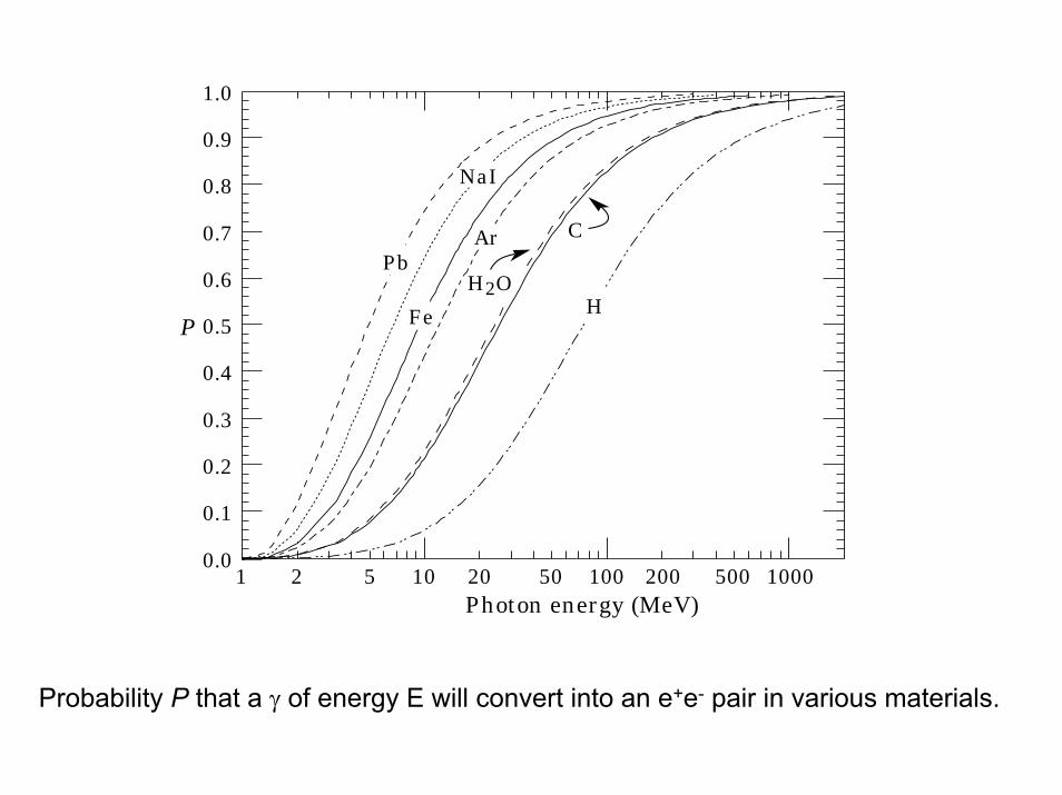
Probability P that a γ of energy E will convert into an e+e- pair in various materials.

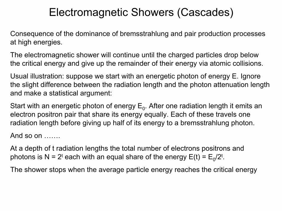
Electromagnetic Showers (Cascades)

Consequence of the dominance of bremsstrahlung and pair production processes at high energies.

The electromagnetic shower will continue until the charged particles drop below the critical energy and give up the remainder of their energy via atomic collisions.

Usual illustration: suppose we start with an energetic photon of energy E. Ignore the slight difference between the radiation length and the photon attenuation length and make a statistical argument:

Start with an energetic photon of energy E0. After one radiation length it emits an electron positron pair that share its energy equally. Each of these travels one radiation length before giving up half of its energy to a bremsstrahlung photon.

And so on …….

At a depth of t radiation lengths the total number of electrons positrons and photons is N = 2t each with an equal share of the energy E(t) = E0/2t.

The shower stops when the average particle energy reaches the critical energy

e−

e−

γ

01 X

Absorber Active medium (scintillation or ionization)

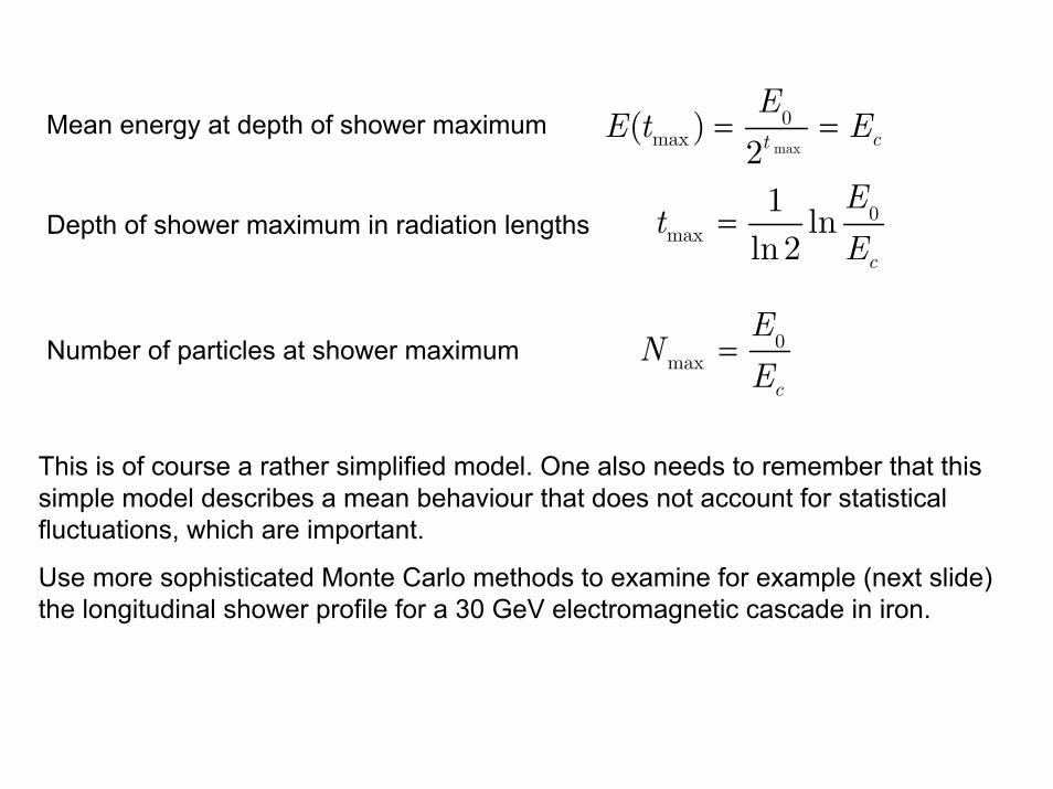
= 0max

c

EN

E

= 0max

1 lnln2 c

Et

E

= =max

0max( )

2 ct

EE t E

This is of course a rather simplified model. One also needs to remember that this simple model describes a mean behaviour that does not account for statistical fluctuations, which are important.

Use more sophisticated Monte Carlo methods to examine for example (next slide) the longitudinal shower profile for a 30 GeV electromagnetic cascade in iron.

Mean energy at depth of shower maximum

Depth of shower maximum in radiation lengths

Number of particles at shower maximum

Monte Carlo Simulation of Electromagnetic Cascade

0.000

0.025

0.050

0.075

0.100

0.125

0

20

40

60

80

100

(1/

E0)

dE

/d

t

t = depth in radiation lengths

Nu

mbe

r cr

ossi

ng

plan

e

30 GeV electronincident on iron

Energy

Photons× 1/6.8

Electrons

0 5 10 15 20

− −

=Γ

1

0

( )( )

a btdE bt eE bdt a

Distribution well fit by gamma dist.

a, b depend on material

γ

γ

= −

= × + =

= − = + =

max ( 1)/

1.0 (ln ) ,

0.5, 0.5, /i

e c

t a b

y C i e

C C y E E

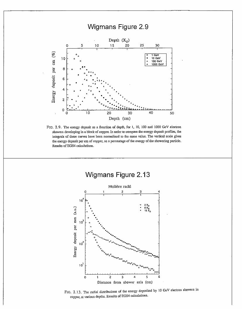
See also Figure 2.9 in Wigmans for longitudinal profiles of electron-induced electromagnetic showers in copper.

Amount of material required to contain a factor of 10 more energy is rather small. Thickess of material required for containment goes like ln E. Important for detector design….tracker size often scales linearly with E.

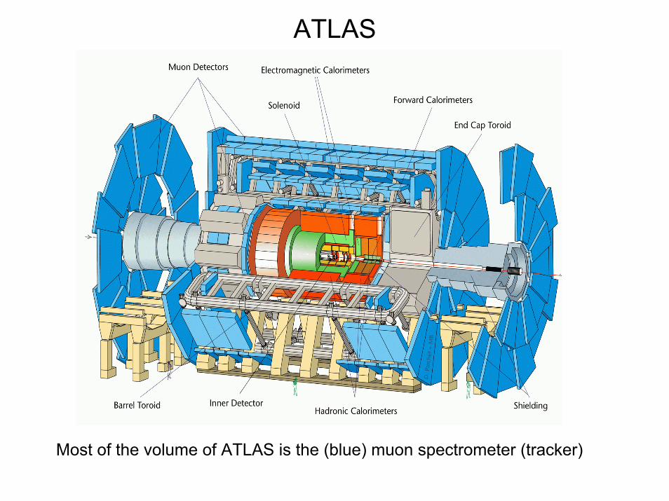
ATLAS

Most of the volume of ATLAS is the (blue) muon spectrometer (tracker)

Transverse Shower Development

= 0 /s cMR X E E [where Es = 21 MeV]

On average, only 10% of the deposited energy lies outside the cylinder with radius RM. About 99% is contained within 3.5 RM

Both longitudinal and transverse shower development are important issues in calorimeter design, which you will learn about later in the course (for example longitudinal and transverse containment, out of cone energy in jet-finding algorithms, choices about segmentation etc.)

As shower progresses, the lateral size will also increase due to a variety of effects:

finite opening angle between e+e- in pair production

emission of bremsstrahlung photons away from the longitudinal axis (which can then travel some distance before interacting).

multiple scattering of electrons and positrons

The transverse shower dimensions are most conveniently measured in terms of the Moliere radius

See also Figure 2.13 in Wigmans (transverse shower development in copper)

Electromagnetic Shower Profiles

Expressed in terms of X0 and ρM the development of electromagnetic showers is approximately material independent.

See Wigmans section 2.1.6 and Figure 2.12 and 2.14 showing longitudinal profiles for 10 GeV electron showers in aluminum, iron and lead.

Differences are attributable to low-energy effects, differences in Ec for different materials.

Ec = 7 MeV for Pb, 22 MeV for Fe and 43 MeV for Al and so shower maximum is deeper in higher Z (lower Ec) materials. This explanation of the longer tail in Pb is similar.

Explanation for differences in the transverse profiles are similar