interaction effects and group comparisons

Interaction effects and group comparisons

Interaction effects and group comparisons Richard Williams, University of Notre Dame, https://www3.nd.edu/~rwilliam/

Last revised February 20, 2015 Note: This handout assumes you understand factor variables, which were introduced in Stata 11. If not, see the first appendix on factor variables. The other appendices are optional. If you are using an older version of Stata or are using a Stata program that does not support factor variables see the appendix on Interaction effects the old fashioned way; also, the appendices on the nestreg command (which does not support factor variables) and the xi prefix (an older alternative to the use of factor variables) may also be useful. Finally, there is an appendix that shows the equivalences between t-tests and one-way ANOVA with a regression model that only has dummy variables. Also, there are a lot of equations in the text, e.g. for calculations of incremental F tests. You can just skip over most of these if you are content to trust Stata to do the calculations for you. Alternative strategy for testing whether parameters differ across groups: Dummy variables and interaction terms. We have previously shown how to do a global test of whether any coefficients differ across groups. This can be a good starting point in that it tells us whether any differences exist across groups. It may also be useful when we have good reason for believing that the models for two or more groups are substantially different. This approach, however, has some major limitations. First, it does not tell you which coefficients differ across groups. Possibilities include (a) only the intercepts differ across groups (b) the intercepts and some subset of the slope coefficients differ across groups, or (c) all of the coefficients, both intercepts and slope coefficients, differ across groups. A related problem is that running separate models for each group can be quite unwieldy, estimating many more coefficients than may be necessary. It becomes even more unwieldy if there are multiple group characteristics you are interested in, e.g. race, gender and religion. Recall that, when extraneous parameters are estimated, it becomes more difficult to detect those effects that really do differ from zero. Further, theory may give you good reason for believing that the effects of only a few variables may differ across groups, rather than all of them. In this handout, we consider an alternative strategy for examining group differences that is generally easier and more flexible. Specifically, by incorporating dummy variables for group membership and interaction terms for group membership with other independent variables, we can better identify what effects, if any, differ across groups.

http://www3.nd.edu/%7Erwilliam/


Model 0/Baseline Model: No differences across groups. As before, we can begin with a model that does not allow for any differences in model parameters across groups.

. use https://www3.nd.edu/~rwilliam/statafiles/blwh.dta, clear

. reg income educ jobexp Source | SS df MS Number of obs = 500 -------------+------------------------------ F( 2, 497) = 1103.96 Model | 32798.4018 2 16399.2009 Prob > F = 0.0000 Residual | 7382.84742 497 14.8548238 R-squared = 0.8163 -------------+------------------------------ Adj R-squared = 0.8155 Total | 40181.2493 499 80.5235456 Root MSE = 3.8542 ------------------------------------------------------------------------------ income | Coef. Std. Err. t P>|t| [95% Conf. Interval] -------------+---------------------------------------------------------------- educ | 1.94512 .0436998 44.51 0.000 1.859261 2.03098 jobexp | .7082212 .0343672 20.61 0.000 .6406983 .775744 _cons | -7.382935 .8027781 -9.20 0.000 -8.960192 -5.805678 ------------------------------------------------------------------------------ . est store baseline

Model 1. Only the intercepts differ across groups. To allow the intercepts to differ by race, we add the dummy variable black to the model. . reg income educ jobexp i.black Source | SS df MS Number of obs = 500 -------------+------------------------------ F( 3, 496) = 787.14 Model | 33206.4588 3 11068.8196 Prob > F = 0.0000 Residual | 6974.79047 496 14.0620776 R-squared = 0.8264 -------------+------------------------------ Adj R-squared = 0.8254 Total | 40181.2493 499 80.5235456 Root MSE = 3.7499 ------------------------------------------------------------------------------ income | Coef. Std. Err. t P>|t| [95% Conf. Interval] -------------+---------------------------------------------------------------- educ | 1.840407 .0467507 39.37 0.000 1.748553 1.932261 jobexp | .6514259 .0350604 18.58 0.000 .5825406 .7203111 1.black | -2.55136 .4736266 -5.39 0.000 -3.481921 -1.620798 _cons | -4.72676 .9236842 -5.12 0.000 -6.541576 -2.911943 ------------------------------------------------------------------------------ . est store intonly

There are several ways to test whether the intercepts differ by race. (a) Since there are only two groups, we can look at the t value for black. It is highly significant implying that the intercepts do differ. Note, however, that if there were more than 2 groups, a t test would not be sufficient. (b) We can also do a Wald test. Since only one parameter is being tested, the F value will, as usual, be the square of the corresponding T value. (Since we are using factor variables, you refer to 1.black rather than black).


. test 1.black ( 1) 1.black = 0 F( 1, 496) = 29.02 Prob > F = 0.0000

However, I find that testparm is often a little easier to use, especially if the categorical variables have more than 2 categories. This is because I can just copy part of the syntax that was used in the estimation command, without having to get the numbers correct for coefficients (e.g. 1.black) like I did above. From here on out I will show the commands for both test and testparm but I will only show the output from testparm. . testparm i.black ( 1) 1.black = 0 F( 1, 496) = 29.02 Prob > F = 0.0000

(c) If we aren’t using software that makes life so simple for us, we can compute an incremental F test. In this case, the constrained model is the baseline model, which forced all parameters to be the same for blacks and whites. SSEc = 7383, DFEc = 497, N = 500. The unconstrained model is Model 1, which allows the intercepts to differ. SSEu = 6975, DFEu = 496, N = 500. The incremental F is then

F SSE SSE N KSSE J

R R N KR JJ N K

c u

u

u c

u,

( ) * ( )*

( ) * ( )( ) *

( ) * (. . ) *( . )

.

− − =− − −

=− − −

−

=−

=−−

=

1

2 2

21 1

1

7383 6975 4966975

82642 81626 4961 82642

29 01

Confirming with the ftest command, . ftest intonly baseline Assumption: baseline nested in intonly F( 1, 496) = 29.02 prob > F = 0.0000

You can also do a likelihood ratio test: . lrtest intonly baseline Likelihood-ratio test LR chi2(1) = 28.43 (Assumption: baseline nested in intonly) Prob > chi2 = 0.0000

Interpretation of a Model that allows only the Intercepts to Differ. We’ll simplify things a bit and consider the case where there is only one X variable. Suppose Y is regressed on X1 and Dummy1, where X1 is a continuous variable and Dummy1 is coded 1 if respondent is a member of group 1, 0 otherwise. Note that there are no interaction terms in the model. In this case, the model assumes that X1 has the same effect, i.e. slope, for both groups. However, the intercept is


different for group 1 than for others. The coefficient for Dummy1 tells you how much higher (or lower) the intercept is for group 1. Put another way, the reported intercept is the intercept for those not in Group 1; the intercept + bdummy1 is the intercept for group 1. For example, suppose that a = 0, b1 = 3, bdummy1 = 2. Graphically, this looks something like

That is, you get two parallel lines; but, for each value of X, the predicted value of Y is 2 units higher for group 1 than it is for group 2.

Such a model implies some sort of flat “advantage” or “disadvantage” for members of group 1. For example, if Y was income and X was education, this kind of model would suggest that, for blacks and whites with equal levels of education, whites will average $2,000 a year more. For both blacks and whites, however, each year of education is worth an additional $3,000 on average. Hence, whites with 10 years of education will average $2,000 more a year than blacks with 10 years of education, whites with 12 years of education will average $2,000 more a year than blacks with 12 years of education, etc.

If there are more than two groups, you can just include additional dummy terms, and add additional parallel lines to the above graph.

The T value for the dummy variable tells you whether the intercept for that group differs significantly from the intercept for the reference group.

Here is how we could generate such a graph for our race data using Stata. There are different ways of doing this (e.g. see the graphics in the Appendix on Interaction terms the old fashioned way). I am going to use the margins command (whose output can be hard to read so I won’t show it, but try it on your own) and the marginsplot command (which, as you might guess, is graphically displaying all the numbers that were generated by margins).

. est restore intonly (results intonly are active now) . quietly margins black, at (jobexp = (1(1)21)) atmeans . marginsplot, noci scheme(sj) name(intonly_jobexp)


Variables that uniquely identify margins: jobexp black

This graph plots the relationship between job experience and income for values of job experience that range between 1 year and 21 years (the observed range in the data). More specifically, because education is also in the model and I specified the atmeans option, it plots the relationship between job experience and income for individuals who have average values of education (13.16 years). I could have used some other value for education but doing so would have simply shifted both lines up or down by the same amount. As you see we get two parallel lines with the black line always 2.55 points below the white line. Doing the same thing for education, . quietly margins black, at (educ = (2(1)21)) atmeans . marginsplot, noci ylabel(#10) scheme(sj) name(intonly_educ) Variables that uniquely identify margins: educ black

1520

2530

35Li

near

Pre

dict

ion

1 2 3 4 5 6 7 8 9 10 11 12 13 14 15 16 17 18 19 20 21jobexp

white black

Adjusted Predictions of black

510

1520

2530

3540

45Li

near

Pre

dict

ion

2 3 4 5 6 7 8 9 10 11 12 13 14 15 16 17 18 19 20 21educ

white black



Again you see two parallel lines with the black line 2.55 points below the white line. (Note that the Y axis is different in the two graphs – because education has a stronger effect than job experience it produces a wider range of predicted values – but the distance between the parallel lines is the same in both graphs.)

Model 2. Intercepts and one or more (but not all) slope coefficients differ across groups. We will now regress Y on the IVs, black, and one interaction term. For reasons we will explain later, when using interaction terms you should generally include the variables that were used to compute the interaction, even if their effects are not statistically significant. In this case, this would mean including black and the IV that was used in computing the interaction term. Here is the Stata output for our current example, where we test to see if the effect of Job Experience is different for blacks and whites:

. reg income educ jobexp i.black i.black#c.jobexp Source | SS df MS Number of obs = 500 -------------+------------------------------ F( 4, 495) = 604.39 Model | 33352.2559 4 8338.06397 Prob > F = 0.0000 Residual | 6828.99339 495 13.7959462 R-squared = 0.8300 -------------+------------------------------ Adj R-squared = 0.8287 Total | 40181.2493 499 80.5235456 Root MSE = 3.7143 -------------------------------------------------------------------------------- income | Coef. Std. Err. t P>|t| [95% Conf. Interval] ---------------+---------------------------------------------------------------- educ | 1.834776 .0463385 39.60 0.000 1.743732 1.925821 jobexp | .7128145 .0395293 18.03 0.000 .6351486 .7904805 1.black | .4686862 1.040728 0.45 0.653 -1.576103 2.513475 | black#c.jobexp | 1 | -.2556117 .0786289 -3.25 0.001 -.4100993 -.1011242 | _cons | -5.514076 .9464143 -5.83 0.000 -7.373561 -3.654592 -------------------------------------------------------------------------------- . est store intjob

The significant negative coefficient for black#c.jobexp indicates that blacks benefit less from job experience than do whites. Specifically, each year of job experience is worth about $256 less for a black than it is for a white.

Doing an incremental F test, we contrast the “unconstrained” model (immediately above) with the constrained model in which blackjob is excluded. (Note that Model 1 is now the constrained model; it is constrained in that the effect of jobexp is constrained to be the same across groups. Remember, the terms constrained and unconstrained are always relative, and that the unconstrained model in one contrast may the constrained model in another.)

SSEu = 6829, R2u = .83005, K = 4.

SSEc = 6975, R2u = .82642, J = 1.


F SSE SSE N KSSE J

R R N KR JJ N K

c u

u

u c

u,

( ) * ( )*

( ) * ( )( ) *

( ) * (. . ) *( . )

.

− − =− − −

=− − −

−

=−

=−−

=

1

2 2

21 1

1

6975 6829 4956829

83005 82642 4951 83005

1058

To confirm,

. ftest intonly intjob Assumption: intonly nested in intjob F( 1, 495) = 10.57 prob > F = 0.0012

The incremental F = the squared T value for blackjob. Or, doing a Wald test with the test or testparm command,

. test 1.black#c.jobexp (Output not shown)

. testparm i.black#c.jobexp ( 1) 1.black#c.jobexp = 0 F( 1, 495) = 10.57 Prob > F = 0.0012

Or, doing a likelihood ratio test,

. lrtest intonly intjob Likelihood-ratio test LR chi2(1) = 10.56 (Assumption: intonly nested in intjob) Prob > chi2 = 0.0012

Interpreting a Model in which the slopes are allowed to differ across groups. Suppose Y is regressed on X1, Dummy1, and Dummy1 * X1. The coefficient for Dummy1 * X1 will indicate how the effect of X1 differs across groups. For example, if the coefficient is positive, this means that X1 has a larger effect (i.e. more positive or less negative) in group 1 than it does in the other group. For example, we might think that whites gain more from each year of education than do blacks. Or, we might even think that the effect of a variable is positive in one group and zero or negative in another. The coefficient for X1 is the effect (i.e. slope) of X1 for those not in group 1; b1 + bdummyX1 is the effect (slope) of X1 on those in group 1. When interaction terms are added, lines are no longer parallel, and you get something like


For both groups, as X increases, Y increases. However, the increase (slope) is much greater for group 1 than it is for group 2.

The T value for the interaction term tells you whether the slope for that group differs significantly from the slope for the reference group.

To generate such a graph in Stata,

. quietly margins black, at (jobexp = (1(1)21)) atmeans

. marginsplot, noci scheme(sj) name(intjob_jobexp) Variables that uniquely identify margins: jobexp black

At low levels of job experience, there is virtually no difference between blacks and whites (people with little experience don’t make much money no matter what their race is). As job experience goes up, the gap between blacks and whites gets bigger and bigger, because whites benefit more from job experience than blacks do. Model 3: All coefficients freely differ across groups. Before, we estimated separate models for blacks and whites. We can achieve the same thing by estimating a model that includes a

2025

3035

Line

ar P

redi

ctio

n

1 2 3 4 5 6 7 8 9 10 11 12 13 14 15 16 17 18 19 20 21jobexp

white black



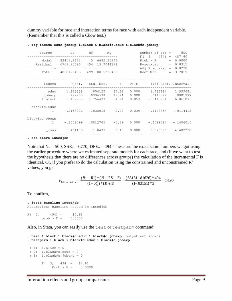
dummy variable for race and interaction terms for race with each independent variable. (Remember that this is called a Chow test.) . reg income educ jobexp i.black i.black#c.educ i.black#c.jobexp Source | SS df MS Number of obs = 500 -------------+------------------------------ F( 5, 494) = 487.60 Model | 33411.2623 5 6682.25246 Prob > F = 0.0000 Residual | 6769.98696 494 13.7044271 R-squared = 0.8315 -------------+------------------------------ Adj R-squared = 0.8298 Total | 40181.2493 499 80.5235456 Root MSE = 3.7019 -------------------------------------------------------------------------------- income | Coef. Std. Err. t P>|t| [95% Conf. Interval] ---------------+---------------------------------------------------------------- educ | 1.893338 .054125 34.98 0.000 1.786994 1.999681 jobexp | .722255 .0396598 18.21 0.000 .6443322 .8001777 1.black | 3.409988 1.756477 1.94 0.053 -.0410984 6.861075 | black#c.educ | 1 | -.2153886 .1038015 -2.08 0.039 -.4193354 -.0114418 | black#c.jobexp | 1 | -.3002799 .0812705 -3.69 0.000 -.4599584 -.1406015 | _cons | -6.461189 1.0479 -6.17 0.000 -8.520079 -4.402298 -------------------------------------------------------------------------------- . est store intedjob

Note that Nu = 500, SSEu = 6770, DFEu = 494. These are the exact same numbers we got using the earlier procedure where we estimated separate models for each race, and (if we want to test the hypothesis that there are no differences across groups) the calculation of the incremental F is identical. Or, if you prefer to do the calculation using the constrained and unconstrained R2 values, you get

F R R N KR KK N K

u c

u+ − − =

− − −− +

=−−

=1 2 2

2 2

22 2

1 183151 81626 494

1 83151 314 90,

( ) * ( )( ) * ( )

(. . ) *( . ) *

.

To confirm,

. ftest baseline intedjob Assumption: baseline nested in intedjob F( 3, 494) = 14.91 prob > F = 0.0000

Also, in Stata, you can easily use the test or testparm command:

. test 1.black 1.black#c.educ 1.black#c.jobexp (output not shown)

. testparm i.black i.black#c.educ i.black#c.jobexp ( 1) 1.black = 0 ( 2) 1.black#c.educ = 0 ( 3) 1.black#c.jobexp = 0 F( 3, 494) = 14.91 Prob > F = 0.0000


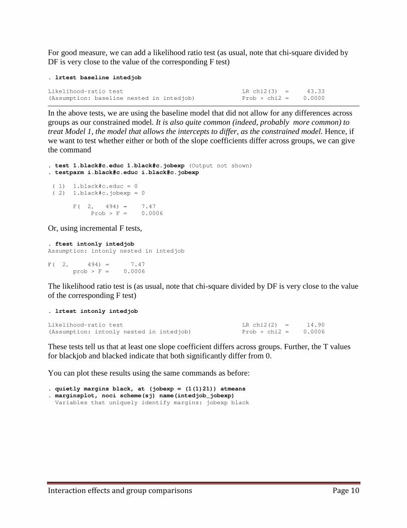
For good measure, we can add a likelihood ratio test (as usual, note that chi-square divided by DF is very close to the value of the corresponding F test)

. lrtest baseline intedjob Likelihood-ratio test LR chi2(3) = 43.33 (Assumption: baseline nested in intedjob) Prob > chi2 = 0.0000

In the above tests, we are using the baseline model that did not allow for any differences across groups as our constrained model. It is also quite common (indeed, probably more common) to treat Model 1, the model that allows the intercepts to differ, as the constrained model. Hence, if we want to test whether either or both of the slope coefficients differ across groups, we can give the command

. test 1.black#c.educ 1.black#c.jobexp (Output not shown)

. testparm i.black#c.educ i.black#c.jobexp ( 1) 1.black#c.educ = 0 ( 2) 1.black#c.jobexp = 0 F( 2, 494) = 7.47 Prob > F = 0.0006

Or, using incremental F tests,

. ftest intonly intedjob Assumption: intonly nested in intedjob F( 2, 494) = 7.47 prob > F = 0.0006

The likelihood ratio test is (as usual, note that chi-square divided by DF is very close to the value of the corresponding F test)

. lrtest intonly intedjob Likelihood-ratio test LR chi2(2) = 14.90 (Assumption: intonly nested in intedjob) Prob > chi2 = 0.0006

These tests tell us that at least one slope coefficient differs across groups. Further, the T values for blackjob and blacked indicate that both significantly differ from 0.

You can plot these results using the same commands as before:

. quietly margins black, at (jobexp = (1(1)21)) atmeans

. marginsplot, noci scheme(sj) name(intedjob_jobexp) Variables that uniquely identify margins: jobexp black


. quietly margins black, at (educ = (2(1)21)) atmeans . marginsplot, noci ylabel(#10) scheme(sj) name(intedjob_educ) Variables that uniquely identify margins: educ black

Comparing the two approaches. Now, let’s compare these with our earlier results from when we ran separate models by race:

Variable/Model Interactions Whites only Blacks Only EDUC 1.893338 1.893338 1.677949 BLACKED -.215389 JOBEXP .722255 .722255 .421975 BLACKJOB -.300280 (Constant) -6.461190 -6.461190 -3.051201 BLACK 3.409989

2025

3035

Line

ar P

redi

ctio

n

1 2 3 4 5 6 7 8 9 10 11 12 13 14 15 16 17 18 19 20 21jobexp

white black

Adjusted Predictions of black20

2530

35Li

near

Pre

dict

ion

1 2 3 4 5 6 7 8 9 10 11 12 13 14 15 16 17 18 19 20 21jobexp

white black



Notice that the coefficients in the interactions model for the intercept, Educ, and Jobexp, are the same as the coefficients we got in the earlier whites-only equation. Further, if you add the interactions model coefficients for Intercept + Black, Educ + Blacked, and Jobexp + Blackjob, you get the coefficients from the earlier blacks-only equation.

Why this works [read on your own if we don’t have time in class]. The model with interaction terms represents an alternative way of expressing the unconstrained model; instead of running separate regressions for each group, we run a single regression, with additional variables. The coefficients for the dummy variable and the interaction terms indicate whether the groups differ or not. With the interactions approach, the unconstrained model can be written as

Y X X Dummy Dummy X Dummy Xdummy dummy X dummy X= + + + + + +α β β β β β ε1 1 2 2 1 21 2* *( * ) ( * )

But, for Group 0, Dummy and the interaction terms computed from it all equal 0; hence for group 0 this simplifies too

Y X X

X X

= + + +

= + + +

α β β ε

α β β ε

1 1 2 2

010

1 20

2( ) ( ) ( )

That is, both the model using interaction terms, and the separate model estimated only for group 0, will yield identical estimates of the intercept and the non-interaction terms (also known as the “main” effects).

For group 1, where Dummy = 1, DUMMYX1 = X1, and DUMMYX2 = X2, the model simplifies to

Y X X X XX X

X X

dummy dummy X dummy X

dummy dummy X dummy X

= + + + + + +

= + + + + + +

= + + +

α β β β β β ε

α β β β β β ε

α β β ε

1 1 2 2 1 1 2 2

1 1 1 2 2 2

11

11 2

12

* *

* *

( ) ( ) ( )

( ) ( ) ( )

That is, adding the “main” effect to the corresponding interaction term gives you the parameters for when a regression is run on Group 1 separately.

The following tables illustrate how to go from parameters estimated using one approach to parameters estimated using the other:


Separate regressions Interactions model

α(0) α

β1(0) β1

β2(0) β2

α(1) - α(0) βdummy

β1(1) - β1

(0) βdummyX1

β2(1) - β2

(0) βdummyX2

As the above make clear,

• The interaction terms indicate the difference in effects between group 1 and group 0. If the intercept is larger in group 1 than in group 0, the coefficient for the dummy variable will be positive. If the effect of a variable is larger (i.e. more positive or less negative) in group 1 than in group 0, then the interaction term will have a positive value.

• If the intercept and regression coefficients are the same in both populations, then the expected values of the interaction terms are all zero. Hence, a test of whether the interaction and dummy terms = zero (which is what the incremental F test is testing) is equivalent to a test of whether there are any group differences.

Other comments on interaction effects and group comparisons • Interpretation of the main effects (i.e. the non-interaction terms) can be a little confusing

when interaction terms are in the model. We’ll discuss these interpretation issues more, and ways to make the interpretation clearer, in a subsequent handout.

• People often get confused by the following: If lines are not parallel, at some point the

group that seems to be “behind” has to have a predicted edge over the other group – although that point may never actually occur within the observed or even any possible data. Consider the following hypothetical example where Education (X) is regressed on Income (Y), with separate lines for men and women:


In the present example, women happen to have a predicted edge over men when education equals 0. They’d have an even bigger edge if you extended the lines to include negative values of job education. But, since you don’t observe such negative and zero values in reality, the predicted lead for women at these values doesn’t mean much.

• Estimating separate models for each group can result in loss of statistical power, i.e. you can be less likely to reject the null when it is false. Similarly, including too many interaction terms can lead to the same problem. As we have seen many times before, inclusion of extraneous variables (in this case, extraneous interaction terms) should be avoided if possible.

• The same model can include interactions involving more than one categorical variable. For example, it might be felt that the effect of education is different for whites than for nonwhites; and, the effect of income is different for women than for men. Hence, the model could include the variables EDUC*WHITE and INCOME*FEMALE. If you have a lot of categorical variables, you should think carefully about what interaction terms to include (if any).

• As noted earlier in the course, a failure to include interactions in models can lead to problems like heteroscedasticity, omitted variable bias, etc.

• One thing to be careful of: When comparing groups by estimating separate models, it is entirely possible that a variable will have a significant effect in one group and an insignificant effect in the other. Yet, the difference in effects between the groups may not be statistically significant. This might occur if, say, the sample size for one group is larger than the sample size for the other. It would therefore be very misleading to say that a variable was important for one group but not the other. Likewise, apparently large differences in effects may not be statistically significant. When comparing groups, you should do formal statistical tests such as those described here if you want to claim there are group differences; don’t rely on just eyeballing.

Male Line

Female Line

X

Y

0


Appendix: Factor Variables (Stata 11 and higher). Factor variables (not to be confused with factor analysis) were introduced in Stata 11. Factor variables provide a convenient means of computing and including dummy variables, interaction terms, and squared terms in models. They can be used with regress and several other (albeit not all) commands. For example, . use https://www3.nd.edu/~rwilliam/statafiles/blwh.dta, clear . reg income i.black educ jobexp Source | SS df MS Number of obs = 500 -------------+------------------------------ F( 3, 496) = 787.14 Model | 33206.4588 3 11068.8196 Prob > F = 0.0000 Residual | 6974.79047 496 14.0620776 R-squared = 0.8264 -------------+------------------------------ Adj R-squared = 0.8254 Total | 40181.2493 499 80.5235456 Root MSE = 3.7499 ------------------------------------------------------------------------------ income | Coef. Std. Err. t P>|t| [95% Conf. Interval] -------------+---------------------------------------------------------------- 1.black | -2.55136 .4736266 -5.39 0.000 -3.481921 -1.620798 educ | 1.840407 .0467507 39.37 0.000 1.748553 1.932261 jobexp | .6514259 .0350604 18.58 0.000 .5825406 .7203111 _cons | -4.72676 .9236842 -5.12 0.000 -6.541576 -2.911943 ------------------------------------------------------------------------------

The i.black notation tells Stata that black is a categorical variable rather than continuous. As the Stata 11 User Manual explains (section 11.4.3.1), “i.group is called a factor variable, although more correctly, we should say that group is a categorical variable to which factor-variable operators have been applied…When you type i.group, it forms the indicators for the unique values of group.” In other words, Stata, in effect, creates dummy variables coded 0/1 from the categorical variable. In this case, of course, black is already coded 0/1 – but margins and other post-estimation commands still like you to use the i. notation so they know the variable is categorical (rather than, say, being a continuous variable that just happens to only have the values of 0/1 in this sample). But if, say, we had the variable race coded 1 = white, 2 = black, the new variable would be coded 0 = white, 1 = black. Or, if the variable religion was coded 1 = Catholic, 2 = Protestant, 3 = Jewish, 4 = Other, saying i.religion would cause Stata to create three 0/1 dummies. By default, the first category (in this case Catholic) is the reference category, but we can easily change that, e.g. ib2.religion would make Protestant the reference category, or ib(last).religion would make the last category, Other, the reference. Factor variables can also be used to include squared terms and interaction terms in models. For example, to add interaction terms,


. reg income i.black educ jobexp black#c.educ black#c.jobexp Source | SS df MS Number of obs = 500 -------------+------------------------------ F( 5, 494) = 487.60 Model | 33411.2623 5 6682.25246 Prob > F = 0.0000 Residual | 6769.98696 494 13.7044271 R-squared = 0.8315 -------------+------------------------------ Adj R-squared = 0.8298 Total | 40181.2493 499 80.5235456 Root MSE = 3.7019 ------------------------------------------------------------------------------ income | Coef. Std. Err. t P>|t| [95% Conf. Interval] -------------+---------------------------------------------------------------- 1.black | 3.409988 1.756477 1.94 0.053 -.0410984 6.861075 educ | 1.893338 .054125 34.98 0.000 1.786994 1.999681 jobexp | .722255 .0396598 18.21 0.000 .6443322 .8001777 | black#c.educ | 1 | -.2153886 .1038015 -2.08 0.039 -.4193354 -.0114418 | black#| c.jobexp | 1 | -.3002799 .0812705 -3.69 0.000 -.4599584 -.1406015 | _cons | -6.461189 1.0479 -6.17 0.000 -8.520079 -4.402298 ------------------------------------------------------------------------------

If you wanted to add a squared term to the model, you could do something like . reg income i.black educ c.educ#c.educ Source | SS df MS Number of obs = 500 -------------+------------------------------ F( 3, 496) = 520.90 Model | 30500.3792 3 10166.7931 Prob > F = 0.0000 Residual | 9680.87009 496 19.5178833 R-squared = 0.7591 -------------+------------------------------ Adj R-squared = 0.7576 Total | 40181.2493 499 80.5235456 Root MSE = 4.4179 ------------------------------------------------------------------------------ income | Coef. Std. Err. t P>|t| [95% Conf. Interval] -------------+---------------------------------------------------------------- 1.black | -6.298638 .5424112 -11.61 0.000 -7.364345 -5.232931 educ | -.5775958 .2176483 -2.65 0.008 -1.005222 -.1499695 | c.educ#| c.educ | .0859208 .0081894 10.49 0.000 .0698305 .1020111 | _cons | 20.41186 1.470897 13.88 0.000 17.5219 23.30181 ------------------------------------------------------------------------------

The # (pronounced cross) operator is used for interactions and product terms. The use of # implies the i. prefix, i.e. unless you indicate otherwise Stata will assume that the variables on both sides of the # operator are categorical and will compute interaction terms accordingly. Hence, we use the c. notation to override the default and tell Stata that educ is a continuous variable. So, c.educ#c.educ tells Stata to include educ^2 in the model; we do not want or need to compute the variable separately. Similarly, i.race#c.educ produces the race * educ interaction term. Stata also offers a ## notation, called factorial cross. It can save some typing and/or provide an alternative parameterization of the results.


At first glance, the use of factor variables might seem like a minor convenience at best: They save you the trouble of computing dummy variables and interaction terms beforehand. Further, factor variables have some disadvantages, e.g. as of this writing they cannot be used with nestreg or stepwise. The advantages of factor variables become much more apparent when used in conjunction with post-estimation commands such as margins. Note: Not all commands support factor variables. In particular, user-written commands often will not support factor variables, sometimes because the commands were written before Stata 11 came out. Chapters 11 and 25 of the Stata Users Guide provide more information. Or, from within Stata, type help fvvarlist.


Appendix: Interaction Effects the Old Fashioned Way Older versions of Stata do not support factor variables; and even some programs you can use in Stata 12 (especially older user-written programs) do not support factor variables. Therefore you may need to compute the interaction terms yourself. Preliminary Steps. If the dummy variables and interaction terms are not already in our data set, we need to compute them: • Compute a DUMMY variable for group membership. Code it 1 for all members of one of the

groups, 0 for all members of the others. For example, you could do something like

. gen dummy = group == 1 & !missing(group)

Here, dummy will equal 1 if group equals 1. It will equal 0 if group has any other nonmissing value. dummy will be missing if group is missing. Another possible approach:

. tab x, gen(dummy)

If x had 4 categories, this would create dummy1, dummy2, dummy3 and dummy4. You could use the rename command to create clearer names, e.g.

. rename dummy1 catholic

. rename dummy2 protestant

. rename dummy3 jewish

. rename dummy4 other

• Compute interaction terms for the dummy variable and each of the IVs whose effects you think may differ across groups. In Stata, do something like

. gen dummyx1 = dummy * x1

. gen dummyx2 = dummy * x2

[NOTE: If you want, you can think of DUMMY as being an interaction term too. DUMMY = DUMMY*X0, where X0 = 1 for all cases.]

Baseline Model: No differences across groups. As before, we can begin with a model that does not allow for any differences in model parameters across groups. We will also compute the interaction terms that we will need later (the dummy variable black is already in the data set).

. use https://www3.nd.edu/~rwilliam/stats2/statafiles/blwh.dta, clear

. gen blacked = black * educ

. gen blackjob = black * jobexp


. reg income educ jobexp Source | SS df MS Number of obs = 500 -------------+------------------------------ F( 2, 497) = 1103.96 Model | 32798.4018 2 16399.2009 Prob > F = 0.0000 Residual | 7382.84742 497 14.8548238 R-squared = 0.8163 -------------+------------------------------ Adj R-squared = 0.8155 Total | 40181.2493 499 80.5235456 Root MSE = 3.8542 ------------------------------------------------------------------------------ income | Coef. Std. Err. t P>|t| [95% Conf. Interval] -------------+---------------------------------------------------------------- educ | 1.94512 .0436998 44.51 0.000 1.859261 2.03098 jobexp | .7082212 .0343672 20.61 0.000 .6406983 .775744 _cons | -7.382935 .8027781 -9.20 0.000 -8.960192 -5.805678 ------------------------------------------------------------------------------ . est store baseline

Model 1. Only the intercepts differ across groups. To allow the intercepts to differ by race, we add the dummy variable black to the model. . reg income educ jobexp black Source | SS df MS Number of obs = 500 -------------+------------------------------ F( 3, 496) = 787.14 Model | 33206.4588 3 11068.8196 Prob > F = 0.0000 Residual | 6974.79047 496 14.0620776 R-squared = 0.8264 -------------+------------------------------ Adj R-squared = 0.8254 Total | 40181.2493 499 80.5235456 Root MSE = 3.7499 ------------------------------------------------------------------------------ income | Coef. Std. Err. t P>|t| [95% Conf. Interval] -------------+---------------------------------------------------------------- educ | 1.840407 .0467507 39.37 0.000 1.748553 1.932261 jobexp | .6514259 .0350604 18.58 0.000 .5825406 .7203111 black | -2.55136 .4736266 -5.39 0.000 -3.481921 -1.620798 _cons | -4.72676 .9236842 -5.12 0.000 -6.541576 -2.911943 ------------------------------------------------------------------------------ . est store intonly

To do Wald and F tests of the effect of black, . test black ( 1) black = 0 F( 1, 496) = 29.02 Prob > F = 0.0000

. ftest intonly baseline Assumption: baseline nested in intonly F( 1, 496) = 29.02 prob > F = 0.0000

Here is how we could generate such a graph for our race data using Stata (note that I am only using jobexp and not educ; on average blacks earn $10,300 less than whites with comparable levels of job experience):


. reg income jobexp black Source | SS df MS Number of obs = 500 -------------+------------------------------ F( 2, 497) = 98.60 Model | 11414.229 2 5707.11449 Prob > F = 0.0000 Residual | 28767.0203 497 57.8813285 R-squared = 0.2841 -------------+------------------------------ Adj R-squared = 0.2812 Total | 40181.2493 499 80.5235456 Root MSE = 7.608 ------------------------------------------------------------------------------ income | Coef. Std. Err. t P>|t| [95% Conf. Interval] -------------+---------------------------------------------------------------- jobexp | .3262549 .0691292 4.72 0.000 .1904335 .4620764 black | -10.30386 .8739031 -11.79 0.000 -12.02086 -8.586861 _cons | 25.43981 1.04632 24.31 0.000 23.38405 27.49556 ------------------------------------------------------------------------------ . predict whiteline if !black (option xb assumed; fitted values) (100 missing values generated) . predict blackline if black (option xb assumed; fitted values) (400 missing values generated) . label variable whiteline "Line for whites" . label variable blackline "Line for blacks" . twoway connected whiteline blackline jobexp

1520

2530

35

0 5 10 15 20jobexp

Line for whites Line for blacks


Model 2. Intercepts and one or more (but not all) slope coefficients differ across groups. . reg income educ jobexp black blackjob Source | SS df MS Number of obs = 500 -------------+------------------------------ F( 4, 495) = 604.39 Model | 33352.2559 4 8338.06397 Prob > F = 0.0000 Residual | 6828.99339 495 13.7959462 R-squared = 0.8300 -------------+------------------------------ Adj R-squared = 0.8287 Total | 40181.2493 499 80.5235456 Root MSE = 3.7143 ------------------------------------------------------------------------------ income | Coef. Std. Err. t P>|t| [95% Conf. Interval] -------------+---------------------------------------------------------------- educ | 1.834776 .0463385 39.60 0.000 1.743732 1.925821 jobexp | .7128145 .0395293 18.03 0.000 .6351486 .7904805 black | .4686862 1.040728 0.45 0.653 -1.576102 2.513475 blackjob | -.2556117 .0786289 -3.25 0.001 -.4100993 -.1011242 _cons | -5.514076 .9464143 -5.83 0.000 -7.373561 -3.654592 ------------------------------------------------------------------------------ . est store intjob

The significant negative coefficient for BLACKJOB indicates that blacks benefit less from job experience than do whites. Specifically, each year of job experience is worth about $256 less for a black than it is for a white.

Doing an incremental F test, . ftest intonly intjob Assumption: intonly nested in intjob F( 1, 495) = 10.57 prob > F = 0.0012

Or, doing a Wald test with the test command,

. test blackjob ( 1) blackjob = 0 F( 1, 495) = 10.57 Prob > F = 0.0012 To generate a graph of an interaction in Stata (again using jobexp only; note that the effect of job experience for blacks is almost zero here):


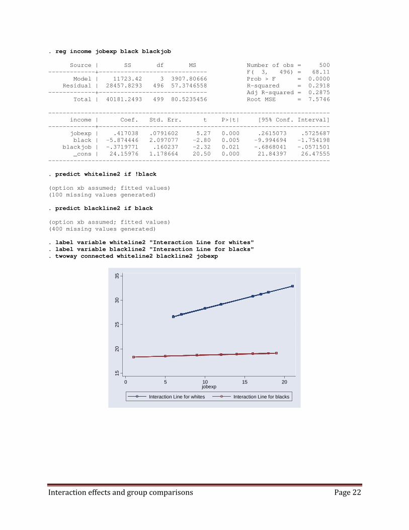
. reg income jobexp black blackjob Source | SS df MS Number of obs = 500 -------------+------------------------------ F( 3, 496) = 68.11 Model | 11723.42 3 3907.80666 Prob > F = 0.0000 Residual | 28457.8293 496 57.3746558 R-squared = 0.2918 -------------+------------------------------ Adj R-squared = 0.2875 Total | 40181.2493 499 80.5235456 Root MSE = 7.5746 ------------------------------------------------------------------------------ income | Coef. Std. Err. t P>|t| [95% Conf. Interval] -------------+---------------------------------------------------------------- jobexp | .417038 .0791602 5.27 0.000 .2615073 .5725687 black | -5.874446 2.097077 -2.80 0.005 -9.994694 -1.754198 blackjob | -.3719771 .160237 -2.32 0.021 -.6868041 -.0571501 _cons | 24.15976 1.178664 20.50 0.000 21.84397 26.47555 ------------------------------------------------------------------------------ . predict whiteline2 if !black (option xb assumed; fitted values) (100 missing values generated) . predict blackline2 if black (option xb assumed; fitted values) (400 missing values generated) . label variable whiteline2 "Interaction Line for whites" . label variable blackline2 "Interaction Line for blacks" . twoway connected whiteline2 blackline2 jobexp

1520

2530

35

0 5 10 15 20jobexp

Interaction Line for whites Interaction Line for blacks


Model 3: All coefficients freely differ across groups. . reg income educ jobexp black blacked blackjob Source | SS df MS Number of obs = 500 -------------+------------------------------ F( 5, 494) = 487.60 Model | 33411.2623 5 6682.25246 Prob > F = 0.0000 Residual | 6769.98696 494 13.7044271 R-squared = 0.8315 -------------+------------------------------ Adj R-squared = 0.8298 Total | 40181.2493 499 80.5235456 Root MSE = 3.7019 ------------------------------------------------------------------------------ income | Coef. Std. Err. t P>|t| [95% Conf. Interval] -------------+---------------------------------------------------------------- educ | 1.893338 .054125 34.98 0.000 1.786994 1.999681 jobexp | .722255 .0396598 18.21 0.000 .6443323 .8001777 black | 3.409988 1.756477 1.94 0.053 -.0410983 6.861074 blacked | -.2153886 .1038015 -2.08 0.039 -.4193354 -.0114418 blackjob | -.3002799 .0812705 -3.69 0.000 -.4599584 -.1406015 _cons | -6.461189 1.0479 -6.17 0.000 -8.520079 -4.402298 ------------------------------------------------------------------------------ . est store intedjob

To test whether there are any racial differences in effects, . ftest baseline intedjob Assumption: baseline nested in intedjob F( 3, 494) = 14.91 prob > F = 0.0000

Also, in Stata, you can easily use the test command:

. test black blacked blackjob ( 1) black = 0 ( 2) blacked = 0 ( 3) blackjob = 0 F( 3, 494) = 14.91 Prob > F = 0.0000

Here, we are using the baseline model that did not allow for any differences across groups as our constrained model. It is also quite common (indeed, perhaps more common) to treat Model 1, the model that allows the intercepts to differ, as the constrained model. Hence, if we want to test whether either or both of the slope coefficients differ across groups, we can give the command

. test blackjob blacked ( 1) blackjob = 0 ( 2) blacked = 0 F( 2, 494) = 7.47 Prob > F = 0.0006


Or, using incremental F tests,

. ftest intonly intedjob Assumption: intonly nested in intedjob F( 2, 494) = 7.47 prob > F = 0.0006

This tells us that at least one slope coefficient differs across groups. Further, the T values for blackjob and blacked indicate that both significantly differ from 0.


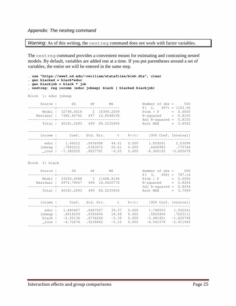
Appendix: The nestreg command Warning: As of this writing, the nestreg command does not work with factor variables. The nestreg command provides a convenient means for estimating and contrasting nested models. By default, variables are added one at a time. If you put parentheses around a set of variables, the entire set will be entered in the same step. . use "https://www3.nd.edu/~rwilliam/statafiles/blwh.dta", clear . gen blacked = black*educ . gen blackjob = black * job . nestreg: reg income (educ jobexp) black ( blacked blackjob) Block 1: educ jobexp Source | SS df MS Number of obs = 500 -------------+------------------------------ F( 2, 497) = 1103.96 Model | 32798.4018 2 16399.2009 Prob > F = 0.0000 Residual | 7382.84742 497 14.8548238 R-squared = 0.8163 -------------+------------------------------ Adj R-squared = 0.8155 Total | 40181.2493 499 80.5235456 Root MSE = 3.8542 ------------------------------------------------------------------------------ income | Coef. Std. Err. t P>|t| [95% Conf. Interval] -------------+---------------------------------------------------------------- educ | 1.94512 .0436998 44.51 0.000 1.859261 2.03098 jobexp | .7082212 .0343672 20.61 0.000 .6406983 .775744 _cons | -7.382935 .8027781 -9.20 0.000 -8.960192 -5.805678 ------------------------------------------------------------------------------ Block 2: black Source | SS df MS Number of obs = 500 -------------+------------------------------ F( 3, 496) = 787.14 Model | 33206.4588 3 11068.8196 Prob > F = 0.0000 Residual | 6974.79047 496 14.0620776 R-squared = 0.8264 -------------+------------------------------ Adj R-squared = 0.8254 Total | 40181.2493 499 80.5235456 Root MSE = 3.7499 ------------------------------------------------------------------------------ income | Coef. Std. Err. t P>|t| [95% Conf. Interval] -------------+---------------------------------------------------------------- educ | 1.840407 .0467507 39.37 0.000 1.748553 1.932261 jobexp | .6514259 .0350604 18.58 0.000 .5825406 .7203111 black | -2.55136 .4736266 -5.39 0.000 -3.481921 -1.620798 _cons | -4.72676 .9236842 -5.12 0.000 -6.541576 -2.911943 ------------------------------------------------------------------------------


Block 3: blacked blackjob Source | SS df MS Number of obs = 500 -------------+------------------------------ F( 5, 494) = 487.60 Model | 33411.2623 5 6682.25246 Prob > F = 0.0000 Residual | 6769.98696 494 13.7044271 R-squared = 0.8315 -------------+------------------------------ Adj R-squared = 0.8298 Total | 40181.2493 499 80.5235456 Root MSE = 3.7019 ------------------------------------------------------------------------------ income | Coef. Std. Err. t P>|t| [95% Conf. Interval] -------------+---------------------------------------------------------------- educ | 1.893338 .054125 34.98 0.000 1.786994 1.999681 jobexp | .722255 .0396598 18.21 0.000 .6443322 .8001777 black | 3.409988 1.756477 1.94 0.053 -.0410984 6.861075 blacked | -.2153886 .1038015 -2.08 0.039 -.4193354 -.0114418 blackjob | -.3002799 .0812705 -3.69 0.000 -.4599584 -.1406015 _cons | -6.461189 1.0479 -6.17 0.000 -8.520079 -4.402298 ------------------------------------------------------------------------------ +-------------------------------------------------------------+ | | Block Residual Change | | Block | F df df Pr > F R2 in R2 | |-------+-----------------------------------------------------| | 1 | 1103.96 2 497 0.0000 0.8163 | | 2 | 29.02 1 496 0.0000 0.8264 0.0102 | | 3 | 7.47 2 494 0.0006 0.8315 0.0051 | +-------------------------------------------------------------+

In the table at the end, Block 1 gives us the statistics for the baseline model in which there are no differences across groups. In effect, you are contrasting a model with no variables with the model that includes educ and jobexp. The F of 1103.96 is therefore the global F statistic for the baseline model. In Block 2, the baseline model is contrasted with the model that allows the intercepts to differ. The F of 29.02 is the F from the Wald test of black (which is the same as the incremental F test). In Block 3, the model that allows only the intercepts to differ is contrasted with the model that also allows the two slope coefficients to differ. The significant F value of 7.47 tells us that at least one of the slope coefficients significantly differs from 0.


Appendix: Y regressed on dummy variables only. Suppose X is a K-category variable with nominal-level measurement. From X, we construct K-1 Dummy variables, e.g. in SPSS

RECODE X (1 = 1) (ELSE = 0) INTO DUMMY1. RECODE X (2 = 1) (ELSE = 0) INTO DUMMY2. RECODE X (3 = 1) (ELSE = 0) INTO DUMMY3.

Note that group 4 is coded 0 on all three dummy variables. Category 4 is sometimes referred to as the excluded category or reference category.

One of several shortcuts for doing this in Stata is

. tab x, gen(dummy)

If x had 4 categories, this would create dummy1, dummy2, dummy3 and dummy4.

If you then regress Y on dummy1, dummy2, dummy3,

• The intercept is the mean for group 4 (i.e. the reference group)

• The intercept + bk is the mean for group k.

• The T values for the betas tell you whether that group’s mean significantly differs from the mean of the excluded category

Note that this is equivalent to a one-way ANOVA, where the dependent variable is Y and the independent variable is X. Or, if X only has 2 values, it is the same as a t-test.

Example: Suppose Religion is coded 1 = Catholic, 2 = Protestant, 3 = Jewish, 4 = Other. If a = 10, b1 = 3, b2 = -2, and b3 = 7, the “other” mean is 10, the Catholic mean is 13, the Protestant mean is 8, and the Jewish mean is 17. The T values for each dummy variable indicate whether the mean for that group significantly differs from the “Other” mean.

For our current example, the average white income is 30.04, the average black income is 18.79, i.e. 11.25 less than the average white income. Running a regression we get

. reg income black Source | SS df MS Number of obs = 500 -------------+------------------------------ F( 1, 498) = 167.76 Model | 10125 1 10125 Prob > F = 0.0000 Residual | 30056.2493 498 60.3539142 R-squared = 0.2520 -------------+------------------------------ Adj R-squared = 0.2505 Total | 40181.2493 499 80.5235456 Root MSE = 7.7688 ------------------------------------------------------------------------------ income | Coef. Std. Err. t P>|t| [95% Conf. Interval] -------------+---------------------------------------------------------------- black | -11.25 .8685758 -12.95 0.000 -12.95652 -9.543475 _cons | 30.04 .3884389 77.34 0.000 29.27682 30.80318 ------------------------------------------------------------------------------


Commands that give equivalent results:

. oneway income black, tabulate | Summary of income black | Mean Std. Dev. Freq. ------------+------------------------------------ white | 30.04 7.7943748 400 black | 18.79 7.6647494 100 ------------+------------------------------------ Total | 27.79 8.9734913 500 Analysis of Variance Source SS df MS F Prob > F ------------------------------------------------------------------------ Between groups 10125 1 10125 167.76 0.0000 Within groups 30056.2493 498 60.3539142 ------------------------------------------------------------------------ Total 40181.2493 499 80.5235456 Bartlett's test for equal variances: chi2(1) = 0.0442 Prob>chi2 = 0.834 . ttest income, by(black) Two-sample t test with equal variances ------------------------------------------------------------------------------ Group | Obs Mean Std. Err. Std. Dev. [95% Conf. Interval] ---------+-------------------------------------------------------------------- white | 400 30.04 .3897187 7.794375 29.27384 30.80616 black | 100 18.79 .7664749 7.664749 17.26915 20.31085 ---------+-------------------------------------------------------------------- combined | 500 27.79 .4013067 8.973491 27.00154 28.57846 ---------+-------------------------------------------------------------------- diff | 11.25 .8685758 9.543475 12.95652 ------------------------------------------------------------------------------ diff = mean(white) - mean(black) t = 12.9522 Ho: diff = 0 degrees of freedom = 498 Ha: diff < 0 Ha: diff != 0 Ha: diff > 0 Pr(T < t) = 1.0000 Pr(|T| > |t|) = 0.0000 Pr(T > t) = 0.0000


Appendix: The Stata xi command.

Stata has some shortcuts for computing dummy variables and interaction terms. In particular, there is the xi (interaction expansion) command. If you have Stata 11 or higher you will probably want to use factor variables instead, although xi can still be helpful for commands that do not support factor variables (although even in those cases I usually prefer to compute the interactions myself). A typical syntax is

. xi: reg income i.black*educ i.black*jobexp i.black _Iblack_0-1 (naturally coded; _Iblack_0 omitted) i.black*educ _IblaXeduc_# (coded as above) i.black*jobexp _IblaXjobex_# (coded as above) Source | SS df MS Number of obs = 500 -------------+------------------------------ F( 5, 494) = 487.60 Model | 33411.2623 5 6682.25246 Prob > F = 0.0000 Residual | 6769.98696 494 13.7044271 R-squared = 0.8315 -------------+------------------------------ Adj R-squared = 0.8298 Total | 40181.2493 499 80.5235456 Root MSE = 3.7019 ------------------------------------------------------------------------------ income | Coef. Std. Err. t P>|t| [95% Conf. Interval] -------------+---------------------------------------------------------------- _Iblack_1 | 3.409988 1.756477 1.94 0.053 -.0410983 6.861074 educ | 1.893338 .054125 34.98 0.000 1.786994 1.999681 _IblaXeduc_1 | -.2153886 .1038015 -2.08 0.039 -.4193354 -.0114418 _Iblack_1 | (dropped) jobexp | .722255 .0396598 18.21 0.000 .6443323 .8001777 _IblaXjobe~1 | -.3002799 .0812705 -3.69 0.000 -.4599584 -.1406015 _cons | -6.461189 1.0479 -6.17 0.000 -8.520079 -4.402298 ------------------------------------------------------------------------------ . test _Iblack_1 _IblaXeduc_1 _IblaXjobex_1 ( 1) _Iblack_1 = 0 ( 2) _IblaXeduc_1 = 0 ( 3) _IblaXjobex_1 = 0 F( 3, 494) = 14.91 Prob > F = 0.0000

The variable names created by xi are fairly logical, but you might still prefer just to compute variables on you own so you can easily get the names you want. (Also, computing them on your own will get rid of all the annoying “dropped” terms in the printout; on the other hand, Stata may be less likely to screw up the computations of the dummy variables and interaction terms than you are!) Also, note that xi includes the lower-order terms, i.e. even though you didn’t explicitly tell it to include the non-interaction terms for educ, jobexp and black, it did; for the SPSS commands that allow similar shortcuts you have to explicitly specify both the main and interaction effect. If you want a little more control over how terms appear in the printout, you can explicitly specify the main effects, e.g.


. xi: reg income educ jobexp i.black i.black*educ i.black*jobexp i.black _Iblack_0-1 (naturally coded; _Iblack_0 omitted) i.black*educ _IblaXeduc_# (coded as above) i.black*jobexp _IblaXjobex_# (coded as above) Source | SS df MS Number of obs = 500 -------------+------------------------------ F( 5, 494) = 487.60 Model | 33411.2623 5 6682.25246 Prob > F = 0.0000 Residual | 6769.98696 494 13.7044271 R-squared = 0.8315 -------------+------------------------------ Adj R-squared = 0.8298 Total | 40181.2493 499 80.5235456 Root MSE = 3.7019 ------------------------------------------------------------------------------ income | Coef. Std. Err. t P>|t| [95% Conf. Interval] -------------+---------------------------------------------------------------- educ | 1.893338 .054125 34.98 0.000 1.786994 1.999681 jobexp | .722255 .0396598 18.21 0.000 .6443323 .8001777 _Iblack_1 | 3.409988 1.756477 1.94 0.053 -.0410983 6.861074 _Iblack_1 | (dropped) educ | (dropped) _IblaXeduc_1 | -.2153886 .1038015 -2.08 0.039 -.4193354 -.0114418 _Iblack_1 | (dropped) jobexp | (dropped) _IblaXjobe~1 | -.3002799 .0812705 -3.69 0.000 -.4599584 -.1406015 _cons | -6.461189 1.0479 -6.17 0.000 -8.520079 -4.402298 ------------------------------------------------------------------------------ . test _Iblack_1 _IblaXeduc_1 _IblaXjobex_1 ( 1) _Iblack_1 = 0 ( 2) _IblaXeduc_1 = 0 ( 3) _IblaXjobex_1 = 0 F( 3, 494) = 14.91 Prob > F = 0.0000

Note: Again, remember that, starting with Stata 11, the xi command still works, but it is often preferable to use factor variables instead.

interaction effects and group comparisons

Documents