intelligent water drops (iwd) algorithm for coquamo ... · isbn: intelligent water drop. s (iwd)...

Intelligent Water Drops (IWD) Algorithm for

COQUAMO Optimization

Abdulelah G. Saif, Safia Abbas, and Zaki Fayed, Member, IAENG

Abstract—Software quality estimation is one of essential

aspects in software projects. Accurate quality estimates are

necessary for goodly developing software systems. Many

estimation methods have been proposed. Among those

methods, COQUAMO, the model used to estimate the

quality of the software project in defects/KSLOC (or some

other unit of size). Nowadays, estimation models are based

on neural network, the fuzzy logic modeling etc. for

accurately estimate software development effort, time and

quality. As, neural networks design have not clear

guidelines and fuzzy logic approach usage is more

difficult, a meta-heuristic Intelligent Water Drops (IWD)

algorithm can offer some improvements in accuracy for

software quality estimation. This work adapts the IWD

algorithm for optimizing the current coefficients of

COQUAMO model to achieve more accurate estimation of

software development quality. The experiment has been

conducted on NASA 93 software projects. This work is the

first one used to optimize COQUAMO.

Index Terms— COQUAMO, IWD algorithm, Software quality estimation

I. INTRODUCTION

A software project that is completed on time, within

budget, and delivers a quality product that satisfies users and

meets requirements is said to be successful. However, many

software projects fail. Only a third of all software

development projects were successful, in terms of they met

budget, schedule, and quality goals as a report given by the

Standish Group states [1]. Most project fails usually are due

to the planning and estimation steps, not due to the

implementation steps. Several studies have been done

during the last decade, for finding the reason of the

software projects failure. 2100 internet sites were searched

extensively by Galorath et al. who found 5000 reasons for

the software project failures. Among the found reasons,

insufficient requirements engineering, poorly planned

project, suddenly decisions making at the early stages of the

project and inaccurate estimations were the most important

reasons [2]. Therefore, accurate software cost, time and

quality estimation is necessary and is critical to both

developers and customers. Software cost estimation focuses

Manuscript submitted July 10, 2015; revised July 22, 2015. The authors

gratefully acknowledge the support of Ain Shams University and Yemen

government in supporting them.

Abdulelah Ghaleb Farhan Saif is Ph.D student at Ain Shams University, Egypt (phone: 00201154415035; [email protected]).

Safia Abbas Mahmoed Abbas is lecturer at Ain Shams University, Egypt (

[email protected]). Zaki Taha Ahmed Fayed is Emeritus Professor at Ain Shams University,

Egypt ( [email protected]).

on the time and the effort required to complete a software

project. Software cost estimation starts at the proposal state

and continues throughout the life time of a project [3]. The

human-effort occupies the large part of software

development cost and most cost estimation methods focus

on this aspect and give estimates in terms of person-month

[4]. Some software defects are unavoidable during software

development, even if accurate planning, well documentation

and proper process control are performed carefully. These

software defects affect the quality of software product which

might be the main cause of project failure [9]. Therefore, in

order to manage budget, schedule and quality of software

projects, several software estimation methods have been

developed. Among those methods, COCOMO II is the

most widely used model for estimating the effort in person-

month and the time in months for the whole software project

and also at different stages, and COQUAMO is the model

used to estimate the quality of the software project in terms

of defects/KSLOC (or some other unit of size). Nowadays,

most estimation models are based on neural network,

genetic algorithm, the fuzzy logic modeling etc. for

accurately estimate software development effort, time and

quality. As, neural networks have not clear guidelines for

design and fuzzy logic approach usage is more difficult, the

meta-heuristic intelligent water drops (IWD) algorithm can

offer some improvements in accuracy for software quality

estimation. This work adapts the IWD algorithm for

optimizing the current coefficients of COQUAMO model to

achieve more accurate estimation of software development

quality. The experiment has been conducted on NASA 93

software projects. This work is the first one used to optimize

COQUAMO.

The rest of the paper is organized as follow: section II

related works, section III COQUAMO model, section IV

dataset description, section V IWD algorithm, section VI

results analysis and section VII discusses and concludes the

paper.

II. RELATED WORK

There are many prediction models that can be used to

predict software defects such as machine learning based

models (artificial neural networks (ANN), Bayesian belief

networks (BBN), reinforcement learning (RL), genetic

algorithms (GA), genetic programming (GP) and decision

trees) [9] and fuzzy logic models [2] etc. However each one

has its own advantages and disadvantages and each one can

be used for specific projects at different stages [9]. Because

COCOMO II is the most widely used and standard model

for estimating the effort in person-month and the time in

months for a software project at different stages [4] and

COQUAMO [10][11] is an extension of it, COQUAMO

Proceedings of the World Congress on Engineering and Computer Science 2015 Vol I WCECS 2015, October 21-23, 2015, San Francisco, USA

ISBN: 978-988-19253-6-7 ISSN: 2078-0958 (Print); ISSN: 2078-0966 (Online)

WCECS 2015

mailto:[email protected]

mailto:%[email protected]



model will deserve much attention to improve it.

Because today's project quality evaluation based on old

coefficients of COQUAMO model may not match the

required accuracy, therefore by calibration, the accuracy of

results in this method will be increased and the aim of this

research is to use IWD algorithm to optimize the current

COQUAMO model coefficients to achieve accurate

software quality estimation and reduce the uncertainty of

COQUAMO coefficients using IWD algorithm.

III. COQUAMO MODEL

Constructive quality model (COQUAMO), which is

shown in figure 1, is an extension of the existing

constructive cost model (COCOMO II) and consists of two

sub-models; defects introduction (DI) sub-model and

defects removal (DR) sub-model.

A. Defect Introduction (DI) Sub-Model

The DI sub-model’s inputs include source lines of code

and/or function points FPs as the sizing parameter, adjusted

for both reuse and breakage, and a set of 21 multiplicative

DI-drivers divided into four categories, platform, product,

personnel and project. These 21 DI-drivers are a subset of

the 22 cost parameters required as input for COCOMO II.

Development flexibility FLEX driver has no effect on defect

introduction and thus here its values for rating are set to 1.

The decision to use these drivers was taken after the

author did an extensive literature search and did some

behavioral analyses on factors affecting defect introduction.

The outputs of DI sub-model are predicted number of non-

trivial defects of requirements, design and code introduced

during development life cycle; where non-trivial defects

include:

Critical (causes a system crash or causes a serious

damage or jeopardizes personnel)

High (causes impairment of critical system

functions and no workaround solution exists)

Medium (causes impairment of critical system

function, though a workaround solution does exist).

Based on expert-judgment, an initial set of values to each

of ratings of the DI-drivers that have an effect on the

number of defects introduced and overall software quality

were proposed and we are used them in our implementation.

B. Defect Removal (DR) Sub- Model

The aim of the defect removal (DR) model is to estimate

the number of defects removed by several defect removal

activities, namely automated analysis AUTA, people

reviews PEER and execution testing and tools EXTT. The

DR model is a post-processor to the DI model. Each of these

three defect removal profiles removes a fraction of the

requirements, design and coding defects introduced from DI

model. Each profile has 6 levels of increasing defect

removal capability, namely ‘Very Low’, ‘Low’, ‘Nominal’,

‘High’, 'Very High' and ‘Extra High’ with ‘Very Low’ being

the least effective and ‘Extra High’ being the most effective

in defect removal.

To determine the defect removal fractions (DRF)

associated with each of the six levels (i.e. very low, low,

nominal, high, very high, extra high) of the three profiles

(i.e. automated analysis, people reviews, execution testing

and tools) for each of the three types of defect artifacts (i.e.

requirements defects, design defects and code defects), the

author conducted a 2-round Delphi and we used the values

of DRF resulted from 2-round Delphi in our

implementation.

The inputs of DR sub-model include software size in

thousand source lines of code KSLOC and/or function

points, defect removal profiles levels and number of non-

trivial defects of requirements (Req), design (Des) and code

(Code) from DI model. For more details about COQUAMO,

see [10] [11].

Fig. 1. Constructive quality model (COQUAMO).

For each of the three artifacts:

Estimated introduced defects in requirements:

DIReq= A1. (Size)B1.

21

1

Re)(j

qjDriverDI ) (1)

Estimated residual defects in Requirements:

DRReq = C1. DIReq.

3

1

Re)1(r

qrDRF (2)

Estimated introduced defects in design:

DIDes=A2. (Size)B2.

21

1

)(j

jDesDriverDI ) (3)

Estimated residual defects in design:

DRDes =C2. DIDes.

3

1

)1(r

rDesDRF (4)

Estimated introduced defects in code:

DICode=A3. (Size)B3.

21

1

)(j

jCodeDriverDI ) (5)

Estimated residual defects in code:

DRCode =C3. DICode.

3

1

)1(r

rCodeDRF (6)

A1, A2, A3, C1, C2 and C3 are the multiplicative

calibration constants for each artifact. Size is the size of the

software project measured in terms of KSLOC (thousands of

source lines of code, function points FPs or any other unit

of size), here KSLOC is converted to FPs as software size

Number of residual defects

(Defect desity per units

of size)

COQUAMO

Software

platform, product,

personnel and

project

attributes

Defect removal

profile levels

Software

size estimate

Defect

Introduction

Sub-Model

Defect

Removal

Sub- Model



WCECS 2015

..

l ..

soil soil soil soil soil soil

..

l

soil

l

soil

soil

soil

soil

soil

..

l ..

..

measure by assuming c language is used for implementation.

B1, B2 and B3 account for economies / diseconomies of

scale. (DI-driver)jReq , (DI-driver)jDes and (DI-

driver)jCode are the defect introduction driver for each

artifact and the jth factor.

r = 1 to 3 for each DR profile, namely automated analysis,

people reviews, execution testing and tools.

DRFrReq, DRFrDes and DRFrCode are Defect Removal

Fraction for defect removal profile r and artifact type (Req,

Des and Code).

IV. DATASET DESCRIPTION

Experiments have been conducted on NASA 93 data set

found in [5]. The dataset consist of 93 completed projects

with its size in kilo line of code (KLOC) and actual quality

in defects/ KLOC. Here KSLOC is converted to FPs as

software size measure by assuming c language is used for

implementation. Multipliers (DI-Drivers) and scale factors

rating from Very Low to Extra High are also given in the

dataset. Defects removal activities levels (ratings) are not

found in NASA 93 dataset, so the ratings are assumed to be

of ‘Nominal’ rating.

In this data set, there is no classification of defects into

requirements (Req), design (Des) and Code (Code) defects,

So the total defects of each project in the dataset are

converted into Req, Des and Code defects according to

Jones report [12] such that documentation defects =0.60 per

function point FP, requirements defects=1 per FP, design

defects =1.25 per FP , code defects=1.75 per FP and bad

fixes defects=0.40.

Therefore, Req, Des and Code defects for each project j

(Prj) in the data set are calculated as follow:

Prj Req defects =128

Pr of defects total j *(1+0.20) (7)

Prj Des defects= 128

Pr of defects total j *(1.5+0.20) (8)

Prj Code defects=128

Pr of defects total j *(1.75+0.20) (9)

Where, documentation defects are divided equally among

artifacts by assumption (0.20 for each). 128 is a factor of c

language to convert SLOC into FPs. Bad fixes defects are

related to DI-drivers.

V. INTELLIGENT WATER DROPS (IWD)

ALGORITHM

In nature, flowing water drops are mostly seen in rivers,

which form huge moving swarms. The paths that a natural

river follows have been created by a swarm of water drops.

while a natural water drop flows from one point of a river

to the next point in the front, Three changes occur during

this transition: the water drop velocity is increased, the

water drop soil is increased, and in between these two

points, soil of the river’s bed is decreased.

Based on these observations, the Intelligent Water Drops

have been introduced. These Intelligent Water Drops or

IWDs flow in a graph of a given optimization problem.

Then, the resulting effect is that the best solution is obtained

for the problem [6, 7].

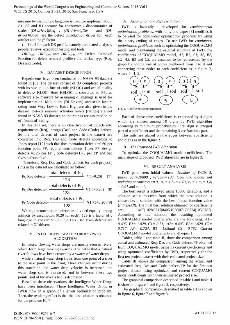
A. Assumption and Representation

IWD is basically developed for combinatorial

optimization problems, with only one paper [8] modifies it

to be used for continuous optimization problems by using

the binary coding of edges. To use IWD for continuous

optimization problems such as optimizing the COQUALMO

model and maintaining the original structure of IWD, the

coefficients of COQUALMO model, A1, B1, C1, A2, B2,

C2, A3, B3 and C3, are assumed to be represented by the

graph by adding virtual nodes numbered from 0 to 9 and

connecting those nodes to each coefficient as in figure 2,

where i= 1..3.

Fig. 2. Coefficients representation.

Each of above nine coefficients is expressed by 4 digits

which are chosen among 10 digits by IWD algorithm

according to minimum probabilities. First digit is integral

part of a coefficient and the remaining 3 are fractions part.

The soils are placed on the edges between coefficients

and digits as in the figure 2.

B. The Proposed IWD Algorithm

To optimize the COQUALMO model coefficients, The

main steps of proposed IWD algorithm are in figure 3.

VI. RESULT ANALYSIS

IWD parameters initial values: Number of IWDs=5,

Initial Soil=10000 , velocity=100, local and global soil

updating parameters=0.9, av = 1,bv = 0.01, cv = 1,as = 1,bs

= 0.01 and cs = 1.

The best result is achieved using 10000 iterations, and a

solution set is received from which the best solution is

chosen i.e. a solution with the best fitness function value

(FitnessAll). The final best solution obtained for coefficients

are: 0405|1028|0717|0405|1028|0717|0724|105|0782|.

According to this solution, the resulting optimized

COQUALMO model coefficients are the following: A1=

0.405, B1= 1.028, C1= 0.71, A2= 0.405, B2= 1.028, C2=

0.717, A3= 0.724, B3= 1.05and C3= 0.782. Current

COQUALMO model coefficients are all equal 1.

Tables, table I and table II, show the comparison among

actual and estimated Req, Des and Code defects/FP obtained

from COQUALMO model using its current coefficients and

using optimized coefficients by IWD, respectively for the

first ten project dataset with their estimated project size.

Table III shows the comparison among the actual and

estimated Req, Des and Code defects/FP for the first ten

project dataset using optimized and current COQUAMO

model coefficients with their estimated project size.

The graphical comparison described in table I and table II

is shown in figure 4 and figure 5, respectively.

The graphical comparison described in table III is shown

in figure 6, figure 7 and figure 8.

Bi Ai Ci

9 0 9 0 9 0



WCECS 2015

1. Set parameters and determine dataset

2. Initialize the soils of virtual edges between coefficients

and their digits.

3. While (termination condition not met) do

4. IWDs are placed on the first node A1 and move to

the next until node C3 is reached.

5. IWDs choose 4 digits among 10 digits as values for

all coefficients according to minimum probabilities

and add the digits to their visited lists. If there is no

improvement in one of the fitness functions

(FitnessCode) in step 10, IWDs choose 4 digits for

each coefficient randomly.

6. IWDs update their velocity

7. IWDs update soils on edges between coefficients and

chosen digits and load some soils according to IWD

algorithm equation 4 in [6].

8. Each IWD i calculate estimated Req, Des and Code

defects for each project j in the dataset using the

values of coefficients chosen by them.

9. Each IWD i calculates Magnitude of Relative Error

(MRE) for each project j, the equation used for Req,

Des and Code, respectively are:

FitnessReqij = | ActualReqj – EstimatedReqij | /

ActualReqj (10)

FitnessDesij = | ActualDesj – EstimatedDesij | /

ActualDesj (11)

FitnessCodeij =|ActualCodej–EstimatedCodesij | /

ActualCodej (12)

10. The fitness functions (Mean Magnitude of Relative

Error MMRE) for each artifact are calculated as the

average value of all projects specific fitness values

calculated during steps 8 and 9 which depends on the

difference between real and estimated Req, Des and

Code defects. So, the fitness functions values should

be minimized.

FitnessReq = 1/n *

n

j 1

FitnessReqij (13)

FitnessDes = 1/n *

n

j 1

FitnessDesij (14)

FitnessCode = 1/n *

n

j 1

FitnessCodeij (15)

FitnessAll=(FitnessReq+FitnessDes+FitnessCode)/3

(16)

11. Find the iteration best solution (optional).

12. Update the soils of virtual edges that form current

best solution according to IWD equation 6 in [6]

(optional).

13. end while.

14. Return the values of coefficients and the estimated Req,

Des and Code defects.

i - the IWD number, j – the project number, ActualReqj - is actual

software Req defects, EstimatedReqij - is the estimated software Req

defects, using IWD i, ActualDesj - is actual software Des defects,

EstimatedDesij - is the estimated software Des defects, using IWD i,

ActualCodej - is actual software Code defects and EstimatedCodesij - is the

estimated software Code defects, using IWD i.

Fig. 3. Proposed IWD algorithm.

TABLE I: ESTIMATED DEVELOPMENT DEFECTS VALUES BY CURRENT

COQUAMO COEFFICIENTS

Pr.

No

FP

s

Act

ual

Req

Def

ects

/FP

Req

Def

ects

/F

P C

alcu

late

d b

y

Cu

rren

t C

OQ

UA

MO

co

effi

cien

ts

Act

ual

Des

Def

ects

/FP

Des

Def

ects

/FP

Cal

cula

ted

by

Cu

rren

t C

OQ

UA

MO

co

effi

cien

ts

Act

ual

Co

de

Def

ects

/FP

Cod

e D

efec

ts /

FP

Cal

cula

ted

by

Cu

rren

t C

OQ

UA

MO

co

effi

cien

ts

1 202.3

4375

7.575 27.18

968

9.153

125

29.48

876

12.30

9375

17.50

53

2 192.1

875

7.190

625

25.82

495

8.688

6719

28.00

863

11.68

4766

16.62

665

3 60.15

625

2.25 8.083

419

2.718

75

8.766

929

3.656

25

5.204

278

4 64.06

25

2.4 8.608

317

2.9 9.336

21

3.9 5.542

218

5 75.78

125

2.831

25

10.18

301

3.421

0938

11.04

405

4.600

7813

6.556

038

6 17.1875

0.646875

2.309548

0.7816406

2.504837

1.0511719

1.486937

7 27.34

375

1.021

875

3.674

282

1.234

7656

3.984

968

1.660

5469

2.365

581

8 520.3125

19.471875

69.91633

23.528516

75.82825

31.641797

45.01362

9 58.59

375

2.118

75

6.333

148

2.560

1563

8.028

77

3.442

9688

4.437

561

10 156.25

5.30625

17.9552

6.4117188

18.78181

8.6226563

11.03867

TABLE II: ESTIMATED DEVELOPMENT DEFECTS VALUES BY OPTIMIZED

IWD COEFFICIENTS

Pr_

No

FP

s

Act

ual

Req

Def

ects

/FP

Req

Def

ects

/FP

Cal

cula

ted

by

Op

tim

ized

IW

D c

oef

fici

ents

Act

ual

Des

Def

ects

/FP

Des

Def

ects

/FP

Cal

cula

ted

by

Op

tim

ized

IW

D c

oef

fici

ents

Act

ual

Co

de

Def

ects

/FP

Cod

e D

efec

ts /

FP

Cal

cula

ted

by

Op

tim

ized

IW

D c

oef

fici

ents

1 202.34375

7.575 9.161126

9.153125

9.935763

12.309375

12.92467

2 192.1

875

7.190

625

8.688

764

8.688

6719

9.423

46

11.68

4766

12.24

437

3 60.15625

2.25 2.632626

2.71875

2.855233

3.65625

3.616345

4 64.06

25

2.4 2.808

519

2.9 3.045

999

3.9 3.863

306

5 75.78125

2.83125

3.337936

3.4210938

3.620182

4.6007813

4.608556

6 17.18

75

0.646

875

0.726

252

0.781

6406

0.787

661

1.051

1719

0.970

506

7 27.34375

1.021875

1.170519

1.2347656

1.269495

1.6605469

1.580251

8 520.3

125

19.47

1875

24.18

846

23.52

8516

26.23

376

31.64

1797

34.84

195

9 58.59375

2.11875

2.061074

2.5601563

2.612901

3.4429688

3.079514

10 156.2

5

5.306

25

6.006

085

6.411

7188

6.282

588

8.622

6563

8.045

497



WCECS 2015

TABLE III: COMPARISON AMONG REQ, DES AND CODE DEFECTS VALUES

VS. SIZE BY IWD AND COQUAMO

Comparison among actual and COQUAMO Req,Des and

Code defecs values vs estimated project size in FPs

0

10

20

30

40

50

60

70

80

202.

3

192.

260

.264

.175

.817

.227

.3

520.

358

.6

156.

3

Project Size (FPs)

Defe

ct/

FP

s

Actual Req Defects/FP

Req Defects /FP

Calculated by Current

COQUAMO coefficients

Actual Des Defects/FP

Des Defects/FP



Actual Code Defects/FP

Code Defects /FP



Fig. 4. Comparison among defects values by COQUAMO.

Comparison among actual and optimized Req,Des and


0

5

10

15

20

25

30

35

40

202.

3

192.

260

.264

.175

.817

.227

.3

520.

358

.6

156.

3

Project Size (FPs)

Defe

ct/

FP

s

Actual Req Defects

Req Defects Calculated

by Optimized IWD

coefficients

Actual Des Defects

Des Defects Calculated

by Optimized IWD

coefficients

Actual Code Defects

Code Defects Calculated

by Optimized IWD

coefficients

Fig. 5. Comparison among defects values by IWD.

Comparison among actual ,optimized and COQUAMO

Req defecs values vs estimated project size in FPs

010203040

50607080

202.

3

192.

260

.264

.175

.817

.227

.3

520.

358

.6

156.

3

Project Size (FPs)

Defe

ct/

FP

s

Actual Req Defects


by Optimized IWD

coefficients


by Current COQUAMO

coefficients

Fig. 6. Comparison among Req defects values by IWD and COQUAMO.


Des defecs values vs estimated project size in FPs

01020

30405060

7080

202.

3

192.

260

.264

.175

.817

.227

.3

520.

358

.6

156.

3

Project Size (FPs)

Defe

ct/

FP

s

Actual Des Defects


by Optimized IWD

coefficients


by Current COQUAMO

coefficients

Fig. 7. Comparison among Des defects values by IWD and COQUAMO.



0

10

20

30

40

50

202.

3

192.

260

.264

.175

.817

.227

.3

520.

358

.6

156.

3

Project Size (FPs)

Defe

ct/

FP

s

Actual Code Defects


by Optimized IWD

coefficients


by Current COQUAMO

coefficients

Fig. 8. Comparison among Code defects values by IWD and

COQUAMO.

Table IV compares the MMRE (Mean Magnitude of

Relative Error) and PRED (.25) (prediction (0.25) which

shows the performance of IWD and COQUAMO in

estimating the Req, Des and Code defects for the whole

dataset.

Pr_

No

FP

s

Act

ual

Req

Def

ects

/FP

Req

Def

ects

/F

P C

alcu

late

d b

y

Op

tim

ized

IW

D c

oef

fici

ents

Req

Def

ects

/FP

C

alcu

late

d b

y C

urr

ent

CO

QU

AM

O c

oef

fici

ents

Act

ual

Des

D

efec

ts/F

P

Des

Def

ects

/FP

C

alcu

late

d b

y

Op

tim

ized

IW

D c

oef

fici

ents

Des

Def

ects

/FP

C

alcu

late

d b

y C

urr

ent

CO

QU

AM

O c

oef

fici

ents

Act

ual

Co

de

Def

ects

/FP

Cod

e D

efec

ts/F

P C

alcu

late

d b

y

Op

tim

ized

IW

D c

oef

fici

ents

Cod

e D

efec

ts /

FP

Cal

cula

ted

by

Cu

rren

t

CO

QU

AM

O c

oef

fici

ents

1 20

2.343

75

7.5

75

9.1

6112

6

27.

1896

8

9.1

5312

5

9.9

3576

3

29.

4887

6

12.

3093

75

12.

9246

7

17.

5053

2 19

2.187

5

7.1

9062

5

8.6

8876

4

25.

8249

5

8.6

8867

19

9.4

2346

28.

0086

3

11.

6847

66

12.

2443

7

16.

6266

5

3 60.15

62

5

2.25

2.632

62

6

8.083

41

9

2.718

75

2.855

23

3

8.766

92

9

3.656

25

3.616

34

5

5.204

27

8

4 64.06

25

2.4 2.808

51

9

8.608

31

7

2.9 3.045

99

9

9.336

21

3.9 3.863

30

6

5.542

21

8

5 75.

78

125

2.8

31

25

3.3

37

936

10.

18

301

3.4

21

0938

3.6

20

182

11.

04

405

4.6

00

7813

4.6

08

556

6.5

56

038

6 17.

18

75

0.6

46

875

0.7

26

252

2.3

09

548

0.7

81

6406

0.7

87

661

2.5

04

837

1.0

51

1719

0.9

70

506

1.4

86

937

7 27.

3437

5

1.0

2187

5

1.1

7051

9

3.6

7428

2

1.2

3476

56

1.2

6949

5

3.9

8496

8

1.6

6054

69

1.5

8025

1

2.3

6558

1

8 520.3

12

5

19.47

18

75

24.18

84

6

69.91

63

3

23.52

85

16

26.23

37

6

75.82

82

5

31.64

17

97

34.84

19

5

45.01

36

2

9 58.59

37

5

2.118

75

2.061

07

4

6.333

14

8

2.560

15

63

2.612

90

1

8.028

77

3.442

96

88

3.079

51

4

4.437

56

1

10 15

6.2

5

5.3

06

25

6.0

06

085

17.

95

52

6.4

11

7188

6.2

82

588

18.

78

181

8.6

22

6563

8.0

45

497

11.

03

867



WCECS 2015

MMRE =n

1 *

n

j 1 j

jj

Actual

| Estimated - Actual| (17)

MREj =Actualj

|Estimatedj-Actualj| (18)

PRED (p) = k / n (19)

k is the number of projects where MRE is less than or

equal to p, and n is the total number of projects.

The graphical comparison described in table IV is shown

in figure 9.

Performance Comparison

0

0.5

1

1.5

2

2.5

MM

RE_R

eq

MM

RE_D

es

MM

RE_C

ode

Tota

l MM

RE

PRED_R

eq (0.

25)

PRED_D

es (0

.25)

PRED_C

ode

(0.2

5)

Tota

l PRED

(0.2

5)

IWD

COQUAMO

Fig. 9. Performance measure comparison.

From table IV and figure 9, the MMRE of IWD for Req,

Des and Code defects is lower than that of COQUAMO and

PRED(0.25) of IWD for Req, Des and Code defects is larger

than that of COQUAMO.

It shows clearly that optimized coefficients by IWD

algorithm produces more accurate results than the old

coefficients. So, IWD algorithm can offer some significant

improvements in accuracy and has the potential to be a valid

additional tool for the software quality estimation

VII. DISCUSSION and CONCLUSION

This paper adapts IWD algorithm for optimizing

COQUAMO coefficients. The proposed algorithm is tested

on NASA 93 dataset and the obtained results are compared

with the ones obtained using the current COQUAMO model

coefficients. The proposed model is able to provide good

estimation capabilities. It is concluded that

By having the appropriate statistical data describing

the software development projects, IWD based

coefficients can be used to produces better results in

comparison with the results obtained using the

current COQUAMO model coefficients.

The results show that, in the sample projects taken

from the dataset, the results obtained using the

coefficients optimized with the proposed algorithm

are better than the ones obtained using the current

coefficients.

The results also show that in the sample projects

taken from the dataset, the results obtained using the

coefficients optimized with the proposed algorithm

are close to the real defects values.

The results also show that in the whole dataset, the

MMRE of IWD is less than that of COQUAMO and

PRED(0.25) is larger than that of COQUAMO.

In the future work or the next paper, we adapt PDBO

algorithm for optimizing the coefficients of COQUAMO

and compare it with IWD algorithm.

REFERENCES

[1] Gary B. Shelly, Harry J. Rosenblatt, “Systems Analysis and Design

Ninth Edition”, Shelly Cashman Series®, 2012.

[2] Vahid Khatibi, Dayang N. A. Jawawi, “ Software Cost Estimation Methods: A Review”, Volume 2 No. 1, Journal of Emerging Trends

in Computing and Information Sciences, 2011.

[3] Sweta Kumari , Shashank Pushkar, “Performance Analysis of the Software Cost Estimation Methods: A Review ”, International Journal

of Advanced Research in Computer Science and Software Engineering, Volume 3, Issue 7, July 2013.

[4] Astha Dhiman, Chander Diwaker, “Optimization of COCOMO II

Effort Estimation using Genetic Algorithm”, American International Journal of Research in Science, Technology, Engineering &

Mathematics, 2013,

[5] Nasa 93 dataset contains effort and defect information available at http://promisedata.googlecode.com/svn/trunk/effort/nasa93-

dem/nasa93-dem.arff.

[6] Hamed Shah-Hosseini, “The intelligent water drops algorithm: a nature-inspired swarm-based optimization algorithm”, Int. J. Bio-

Inspired Computation, Vol. 1, Nos. 1/2, 2009.

[7] Priti Aggarwal, Jaspreet Kaur Sidhu, Harish Kundra,“applications of

intelligent water drops” , IISRO, Multi-Conference, Bangkok, 2013 .

[8] Hamed Shah-Hosseini, “An approach to continuous optimization by

the Intelligent Water Drops algorithm”, 4th International Conference of Cognitive Science (ICCS 2011)

[9] Mrinal Singh Rawat, Sanjay Kumar Dubey, “Software Defect

Prediction Models for Quality Improvement: A Literature Study”, IJCSI International Journal of Computer Science Issues, Vol. 9, Issue

5, No 2, September 2012.

[10] Sunita Chulani, “results of Delphi for the defects introduction model (sub-model of the cost/quality model extension to COCOMO II) ”,

Center for software engineering, 1997.

[11] Sunita Chulani and Barry Boehm, “Modeling Software Defect Introduction and Removal: COQUALMO (Constructive Quality

Model) ”, USC - Center for Software Engineering, Los Angeles, CA

90089-0781, 1999. [12] Capers Jones, “software defect origin and removal methods”, Draft

5.0 , December 28, 2012.

TABLE IV: PERFORMANCE MEASURE COMPARISON

Results IWD COQUAMO

MMRE_Req 0.129249 1.92676

MMRE_Des 0.062069 1.951845

MMRE_Code 0.059168 0.32434

Total MMRE 0.083495 1.400982

PRED_Req (0.25) 0.913978 0

PRED_Des (0.25) 0.989247 0

PRED_Code (0.25) 0.978495 0.204301

Total PRED (0.25) 0.960573 0.0681



WCECS 2015

http://promisedata.googlecode.com/svn/trunk/effort/nasa93-dem/nasa93-dem.arff

http://promisedata.googlecode.com/svn/trunk/effort/nasa93-dem/nasa93-dem.arff

intelligent water drops (iwd) algorithm for coquamo ... · isbn: intelligent water drop. s (iwd)...

Documents