intelligent gait control of a multilegged robot …
TRANSCRIPT
INTELLIGENT GAIT CONTROL OF A MULTILEGGED ROBOT USED
IN RESCUE OPERATIONS
A THESIS SUBMITTED TO
THE GRADUATE SCHOOL OF NATURAL AND APPLIED SCIENCES
OF
THE MIDDLE EAST TECHNICAL UNIVERSITY
BY
EMRE KARALARLI
IN PARTIAL FULFILMENT OF THE REQUIREMENTS FOR THE
DEGREE OF
MASTER OF SCIENCE
IN
THE DEPARTMENT OF ELECTRICAL AND ELECTRONICS
ENGINEERING
DECEMBER 2003
Approval of the Graduate School of Natural and Applied Sciences
——————————————–
Prof. Dr. Canan Ozgen
Director
I certify that this thesis satisfies all the requirements as a thesis for the degree
of Master of Science.
——————————————–
Prof. Dr. Mubeccel Demirekler
Head of Department
This is to certify that we have read this thesis and that in our opinion it is
fully adequate, in scope and quality, as a thesis for the degree of Master of
Science.
——————————————– ——————————————–
Prof. Dr. Ismet Erkmen Assoc. Prof. Dr. Aydan Erkmen
Co-Supervisor Supervisor
Examining Committee Members
Prof. Dr. Erol Kocaoglan ———————————–
Prof. Dr. Aydın Ersak ———————————–
Prof. Dr. Ismet Erkmen ———————————–
Assoc. Prof. Dr. Aydan Erkmen ———————————–
Asst. Prof. Dr. Ilhan Konukseven ———————————–
ABSTRACT
INTELLIGENT GAIT CONTROL OF A MULTILEGGED ROBOT USED
IN RESCUE OPERATIONS
Karalarlı, Emre
M.S., Department of Electrical and Electronics Engineering
Supervisor: Assoc. Prof. Dr. Aydan Erkmen
Co-Supervisor: Prof. Dr. Ismet Erkmen
December 2003, 97 pages
In this thesis work an intelligent controller based on a gait synthesizer
for a hexapod robot used in rescue operations is developed. The gait synthe-
sizer draws decisions from insect-inspired gait patterns to the changing needs
of the terrain and that of rescue. It is composed of three modules responsible
for selecting a new gait, evaluating the current gait, and modifying the rec-
ommended gait according to the internal reinforcements of past time steps. A
Fuzzy Logic Controller is implemented in selecting the new gaits.
Key words: Hexapod Walking Rescue Robots, Insect-inspired Gaits, Gait Syn-
thesizer, GARIC.
iii
OZ
COK BACAKLI KURTARMA ROBOTLARININ AKILLI YURUYUS
DENETIMI
Karalarlı, Emre
Yuksek Lisans, Elektrik ve Elektronik Muhendisligi Bolumu
Tez Yoneticisi: Doc. Dr. Aydan Erkmen
Ortak Tez Yoneticisi: Prof. Dr. Ismet Erkmen
Aralık 2003, 97 sayfa
Bu tez calısmasında kurtarma robotlarının akıllı yuruyus denetimi icin
bir yuruyus sekli sentezleyicisi gelistirilmistir. Sentezleyici degisen zemin
ozelliklerine ve farklı kurtarma calısmalarına cevap verebilmek icin boceklerden
ilham alınan yuruyus sekillerine gore karar vermektedir. Sentezleyici, yuruyus
sekli belirleyici, degerlendirici ve degistirici olmak uzere uc bolumden olusur.
Belirleyici, bir bulanık mantık denetleyicisidir.
Anahtar Sozcukler: Altı Bacaklı Kurtarma Robotları, Boceklerden Ilham
Alınmıs Yuruyus Sekilleri, Yuruyus Sekli Sentezleyicisi, GARIC.
iv
ACKNOWLEDGMENTS
I would like to express my gratitude to my supervisor Assoc. Professor
Dr. Aydan Erkmen and co-supervisor Prof. Dr. Ismet Erkmen for their
motivation, guidance, patience, and encouragement through the preparation
of this thesis. I also thank to all my friends, especially Engur and Aslı Pisirici,
Mehmetcik and Semra Pamuk, Bora Sagdıcoglu, and Sedat Ilgaz for their
invaluable comments and suggestions throughout the study. Finally, I express
my gratitude to my family for their endless support.
v
TABLE OF CONTENTS
ABSTRACT . . . . . . . . . . . . . . . . . . . . . . . . . . . . . . . . . . . . . . . . . . . . . . . . . . . . . . . . . . . . . iii
OZ . . . . . . . . . . . . . . . . . . . . . . . . . . . . . . . . . . . . . . . . . . . . . . . . . . . . . . . . . . . . . . . . . . . . . . . iv
ACKNOWLEDGMENTS . . . . . . . . . . . . . . . . . . . . . . . . . . . . . . . . . . . . . . . . . . . . . . . . . v
TABLE OF CONTENTS . . . . . . . . . . . . . . . . . . . . . . . . . . . . . . . . . . . . . . . . . . . . . . . . .vi
LIST OF FIGURES . . . . . . . . . . . . . . . . . . . . . . . . . . . . . . . . . . . . . . . . . . . . . . . . . . . . .viii
CHAPTER
1. INTRODUCTION . . . . . . . . . . . . . . . . . . . . . . . . . . . . . . . . . . . . . . . . . . . . . . . 1
2. SURVEY . . . . . . . . . . . . . . . . . . . . . . . . . . . . . . . . . . . . . . . . . . . . . . . . . . . . . . . . 7
2.1 Search and Rescue Robotics . . . . . . . . . . . . . . . . . . . . . . . . . . . . . . . . . 7
2.2 Legged Locomotion . . . . . . . . . . . . . . . . . . . . . . . . . . . . . . . . . . . . . . . . . . 8
2.2.1 Walking Mechanisms in Animals . . . . . . . . . . . . . . . . . . . . . . . 8
2.2.2 Control of Legged Robots . . . . . . . . . . . . . . . . . . . . . . . . . . . . . 13
2.2.3 Gait Analysis . . . . . . . . . . . . . . . . . . . . . . . . . . . . . . . . . . . . . . . . . 15
2.2.4 Gait Control . . . . . . . . . . . . . . . . . . . . . . . . . . . . . . . . . . . . . . . . . . 19
2.3 Mathematical Background . . . . . . . . . . . . . . . . . . . . . . . . . . . . . . . . . . 24
2.3.1 Neural-Fuzzy Controllers . . . . . . . . . . . . . . . . . . . . . . . . . . . . . . 24
2.3.2 GARIC Architecture . . . . . . . . . . . . . . . . . . . . . . . . . . . . . . . . . . 25
2.3.3 Fuzzy Sets and Fuzzy Logic Controllers . . . . . . . . . . . . . . . 31
2.3.4 Reinforcement Learning . . . . . . . . . . . . . . . . . . . . . . . . . . . . . . . 34
3. LEGGED ROBOT . . . . . . . . . . . . . . . . . . . . . . . . . . . . . . . . . . . . . . . . . . . . . .37
3.1 Dynamics and Coordinated Control of Legged Robots . . . . . . .37
3.1.1 Motion Dynamics of Legged Robots . . . . . . . . . . . . . . . . . . . 38
vi
3.1.2 Coordinated Control of Legged Robots . . . . . . . . . . . . . . . . 45
3.2 Gait Controller . . . . . . . . . . . . . . . . . . . . . . . . . . . . . . . . . . . . . . . . . . . . . 50
3.2.1 Encoding the Gaits for a Multilegged Robot . . . . . . . . . . .50
3.2.2 Gait Selection Module (GSM) . . . . . . . . . . . . . . . . . . . . . . . . . 57
3.2.3 Gait Evaluation Module (GEM) . . . . . . . . . . . . . . . . . . . . . . .59
3.2.4 Gait Modifier Module (GMM) . . . . . . . . . . . . . . . . . . . . . . . . 60
3.2.5 The Complete Control Cycle . . . . . . . . . . . . . . . . . . . . . . . . . . 62
4. HEXAPOD ROBOT SIMULATION . . . . . . . . . . . . . . . . . . . . . . . . . . . . 64
4.1 Hexapod Model . . . . . . . . . . . . . . . . . . . . . . . . . . . . . . . . . . . . . . . . . . . . .64
4.2 Sensor System . . . . . . . . . . . . . . . . . . . . . . . . . . . . . . . . . . . . . . . . . . . . . . 66
4.3 Kinematics of the Hexapod Robot . . . . . . . . . . . . . . . . . . . . . . . . . . 68
4.4 Uneven Terrain . . . . . . . . . . . . . . . . . . . . . . . . . . . . . . . . . . . . . . . . . . . . . 69
5. SIMULATION RESULTS . . . . . . . . . . . . . . . . . . . . . . . . . . . . . . . . . . . . . . . 71
5.1 Exploration and Exploitation Dilemma in Reinforcement
Learning . . . . . . . . . . . . . . . . . . . . . . . . . . . . . . . . . . . . . . . . . . . . . . . . . . . 72
5.2 Smooth Terrain Tests . . . . . . . . . . . . . . . . . . . . . . . . . . . . . . . . . . . . . . . 74
5.3 Performance on Rough Terrain . . . . . . . . . . . . . . . . . . . . . . . . . . . . . 78
5.4 Task Shapability: A Must for SAR Operations . . . . . . . . . . . . . . 79
6. CONCLUSION . . . . . . . . . . . . . . . . . . . . . . . . . . . . . . . . . . . . . . . . . . . . . . . . . 87
6.1 General . . . . . . . . . . . . . . . . . . . . . . . . . . . . . . . . . . . . . . . . . . . . . . . . . . . . .87
6.2 Future Work . . . . . . . . . . . . . . . . . . . . . . . . . . . . . . . . . . . . . . . . . . . . . . . .89
REFERENCES . . . . . . . . . . . . . . . . . . . . . . . . . . . . . . . . . . . . . . . . . . . . . . . . . . . . . . . . . . 91
APPENDICES
A. SIMULATION PROGRAM CD . . . . . . . . . . . . . . . . . . . . . . . . . . . . . . . . 97
vii
LIST OF FIGURES
FIGURES
2.1 Tripod (A) and tetrapod (B) support patterns (or supportpolygons) formed by contact points of the supporting legs . . . . . . . 9
2.2 Wave gait patterns. Bold lines represent swing phase. L1signifies the left front leg and R3 indicates the right hind leg . . . 16
2.3 Hexapod model. Dashed legs are in swing phase . . . . . . . . . . . . . . . .17
2.4 Summary of coordination mechanisms in the stick insect. Thepattern of coordinating influences among the step generatorsfor the six legs is shown at the left; the arrows indicate thedirection of the influence. The mechanisms are describedbriefly at the right . . . . . . . . . . . . . . . . . . . . . . . . . . . . . . . . . . . . . . . . . . . . . 21
2.5 The GARIC architecture . . . . . . . . . . . . . . . . . . . . . . . . . . . . . . . . . . . . . . . 26
2.6 The action evaluation network . . . . . . . . . . . . . . . . . . . . . . . . . . . . . . . . . 27
2.7 The action selection network . . . . . . . . . . . . . . . . . . . . . . . . . . . . . . . . . . . 29
2.8 General model of a fuzzy logic controller . . . . . . . . . . . . . . . . . . . . . . . 33
3.1 Coordinate frames defined for the legged robot. The coordinateframe Cci is assigned such that the unit vector z is normal tothe contact surface at the point of contact . . . . . . . . . . . . . . . . . . . . . 40
3.2 Architecture of Gait Synthesizer . . . . . . . . . . . . . . . . . . . . . . . . . . . . . . . 51
3.3 Summary of terminology used in gait analysis . . . . . . . . . . . . . . . . . . 52
3.4 Wave gait patterns. Bold lines represent swing phase. L1signifies the left front leg and R3 indicates the right hind leg . . . 53
3.5 Antecedent Labels, fuzzification of individual leg position . . . . . . 54
3.6 Consequent Labels: task share based on operation modes . . . . . . .56
3.7 Gait Selection Module . . . . . . . . . . . . . . . . . . . . . . . . . . . . . . . . . . . . . . . . . 58
3.8 Complete control cycle . . . . . . . . . . . . . . . . . . . . . . . . . . . . . . . . . . . . . . . . . 63
4.1 The hexapod robot used in simulation . . . . . . . . . . . . . . . . . . . . . . . . . .65
viii
4.2 Hexapod model . . . . . . . . . . . . . . . . . . . . . . . . . . . . . . . . . . . . . . . . . . . . . . . . 66
4.3 Each leg is identical and composed of three links. Pink legs arein swing phase whereas blue ones are in stance . . . . . . . . . . . . . . . . . 67
4.4 Two different postures of the robot. Body level of the robot inB is lowered in order to increase reachable space of the legs . . . . 68
4.5 The modelled uneven terrain. Different surface segments can beseen in the figure. The holes on uneven terrain are modelledby surface segments which are deeper than the legs can reach.Notice that the pink leg (swinging) falls into such a segment . . . 70
5.1 Body speed versus time graphs for different scale factor andthreshold values . . . . . . . . . . . . . . . . . . . . . . . . . . . . . . . . . . . . . . . . . . . . . . . 74
5.2 Comparison of resultant gaits when training is done according totwo different reinforcement for speed (first row) and criticalmargin (second row). The first column gives the resultantgaits, second one body speed versus time, and last columnshows critical margin in the direction of motion versus time . . . . 75
5.3 Internal reinforcement versus time . . . . . . . . . . . . . . . . . . . . . . . . . . . . . 76
5.4 Critical margin, Cm(t), versus time . . . . . . . . . . . . . . . . . . . . . . . . . . . . 77
5.5 Leg tip positions on x direction versus time. In order to increasethe critical margin gait synthesizer applies smaller step sizes . . . 78
5.6 Leg tip trajectories of the hexapod on x-z plane with a fixedtripod gait on the defined terrain . . . . . . . . . . . . . . . . . . . . . . . . . . . . . . 81
5.7 Leg tip trajectories of the hexapod on x-z plane with gaitsynthesizer on the defined terrain . . . . . . . . . . . . . . . . . . . . . . . . . . . . . . 82
5.8 Gait of the hexapod robot on uneven terrain. The robotrecovers tripod gait pattern after some time reaching thesmooth terrain . . . . . . . . . . . . . . . . . . . . . . . . . . . . . . . . . . . . . . . . . . . . . . . . . 83
5.9 Gait of the hexapod robot on uneven terrain. The robotrecovers tripod gait faster than the previous one . . . . . . . . . . . . . . . 84
5.10 Critical margin versus time . . . . . . . . . . . . . . . . . . . . . . . . . . . . . . . . . . . . 84
5.11 Leg tip positions on x direction versus time . . . . . . . . . . . . . . . . . . . . 85
5.12 Gait generated by gait synthesizer when leg R1 is missing . . . . . .85
5.13 Gait generated by gait synthesizer in sudden lack of leg R1 . . . . 86
ix
CHAPTER 1
INTRODUCTION
Recent experiences of natural disasters (earthquakes, tornados, floods)
and man-made catastrophes (e.g. urban terrorism) have brought the attention
to the area of search and rescue (SAR) and emergency management. Horrible
devastations and losses have dramatically illustrated the damage that can be
expected to today’s modern industrialized countries despite the technological
progresses in construction techniques [1]. Besides, these experiences showed
that preparedness and emergency response of the governments are inadequate
to deal with these devastations. As a result, people who have died due to
lack of immediate response inevitably forced us to find out better solutions for
search and rescue.
The utilization of autonomous intelligent robots in search and rescue
(SAR) is a new and challenging field of robotics, dealing with tasks in ex-
tremely hazardous and complex disaster environments [2]. Autonomy, high
mobility, robustness, and reconfigurability are critical design issues of res-
cue robotics, requiring dexterous devices equipped with the ability to learn
from prior rescue experience, adaptable to variable types of usage with a wide
enough functionality under different sensing modules, and compliant to en-
vironmental and victim conditions. Intelligent, biologically inspired mobile
robots and, in particular hexapod robots have turned out to be widely used
robot types beside serpentine mechanisms [3]; providing effective, immediate,
and reliable responses to many SAR operations. Aiming at enhancing the
1
quality of rescue and life after rescue, the field of rescue robotics is seeking
shape changing and moreover task shapable intelligent dexterous devices.
The objective of this thesis is to design a gait synthesizer for 6-legged
walking robots with shape-shifting gaits that provide the necessary flexibility
and adaptability needed in the difficult workspaces of rescue missions. The gait
synthesizer is responsible for the locomotion of the robot providing a compro-
mise between mobility and speed while allowing task shapability to use some
legs as manipulators when need arise during rescue. Legged robots are chosen
due to their advantage on rough terrains over their wheeled mobile counter-
parts [4], [5].
Wheeled locomotion is well suited for fast transportation. Wheels change
their point of support and use friction to move forward in an efficient way.
But due to this fact they require a continuous path. So, they require a pre-
constructed terrain, which restricts mobility demands.
On the other hand, legged locomotion offers a significant potential for
mobility over natural rough terrains in comparison to wheeled or tracked lo-
comotion. Because legs can choose footholds to improve traction, to minimize
lurching and to step over obstacles, they can handle with softness, unevenness
of the terrain [4]. Legs can provide the capability of maneuvering within con-
fined areas of space. Unlike wheels, legs change their point of support all at
once so do not need a continuous path. Also, as seen in nature, legs are not
used only for walking. Beside their main function, they are almost in every
external process of animals (as tactile sensors, as manipulators, etc.).
2
However, legged locomotion possesses additional complexity in the coor-
dination control of the legs [6]. The control of a legged robot is a sophisticated
job due to the high number of degrees of freedom offered by the articulated
legs. In the design of a control structure of a legged robot on difficult rough
terrain there are many aspects that have to be dealt with simultaneously and
that also interfere with each other. For example, movements of legs must be
carefully coordinated in order to advance the body without causing feet slip-
page; at each step, an appropriate foothold has to be found; body attitude
must be set according to the terrain profile; keep stability; accomplish a nav-
igation task; etc. Here, a body movement for terrain adaptation may change
the operation space of a leg so that the leg can not reach a chosen foothold that
was within the range beforehand, or inversely, a decision for a modification in
the gait may solve a stability problem. So, while coordinating the movements
of body and legs, the control structure of the legged robot must also handle
such interferences.
In this thesis we focus on the gait control and leg coordination and em-
phasize the potential of redundancy of legs for handling irregularity on terrains
as well as their use as manipulators. In walking robots, coordinating the move-
ments of individual legs in order to maintain a stable gait is one of the main
control tasks. Observations on insect gaits (cockroaches, stick insects) shows
that insects produce sequential movements starting with hind leg protraction
and followed by the middle and front legs, which is called metachronal wave
or wave gait [7]. Among the numerous periodic gaits, the class of wave gaits
is most important because they provide good stability [8]. The tripod gait,
3
which is a member of wave gaits, involves an alternation between right-sided
and left-sided metachronal waves and it is the fastest gait. Gaits arise from
the interaction of individual leg oscillators (step pattern generators) which
govern the stepping of each leg by exchanging the influences of the legs [9].
The information transmitted from the step pattern generator depends upon
the leg’s state (either swing or stance, position and velocity). Here the position
information play a particular central role in coordination. Several researchers
have implemented insect-like controllers for leg coordination ([10], [11]), most
of which oriented to protect the regularity of a fixed gait pattern against per-
turbations.
In this thesis, we work on biologically inspired wave gait patterns. Gait
patterns are patterns of leg coordination which represents relative phases
(swing phase or stance phase) of legs in a statically stable locomotion. These
gaits have different properties from mobility and speed point of views. In our
method we encoded gait pattern cycles from relative positions of the legs and
find the individual leg’s tasks within those gait patterns. The method enables
exploring among many different gait patterns and selecting gait patterns ac-
cording to the different needs to adapt online to terrain conditions. This is the
point where we have required features of intelligent control.
Generalized approximate reasoning-based intelligent control (GARIC)
architecture [12] is one of the realizations of the fusion of the Fuzzy and Neural
technologies guided by feedback from the environment. It presents a method
for learning and tuning fuzzy logic controllers (FLC) through reinforcements
signals. The basic idea behind Fuzzy Logic Controllers (FLC) is to incorporate
4
the ”expert experience” of a human operator in the design of the controller in
controlling a process whose input-output relationship is described by a collec-
tion of fuzzy control rules (IF-THEN rules) involving linguistic variables rather
than a complicated dynamic model [13].
Our gait synthesizer has adapted the GARIC architecture, to our ob-
jective. The gait synthesizer that we develop for serpentine locomotion [3]
and here for hexapod walking consists of three modules. The Gait Evaluation
Module (GEM), acts as a critic and provides advice to the main controller,
based on a multilayer artificial neural network. The Gait Selection Module
(GSM), offers a new gait to be taken by the robot according to a fuzzy con-
troller with rules for different gait patterns in the knowledge base. The Gait
Modifier Module (GMM), changes the gait recommended by the GSM based
on internal reinforcement. This change in the recommended gait is more sig-
nificant for a state if that state does not receive high internal reinforcements.
(i.e. probability of failure is high). On the other hand, if a state receives
high reinforcements, GMM administers small changes to the action selected
by the fuzzy controller embedded in the GSM. This reveals that the action is
performing well so that the GMM recommendation dictates no or only minor
changes to that gait.
The basic contribution of this thesis is the development of an intelligent
task shapable control, based on a gait synthesizer for a hexapod robot upon its
traversal of unstructured workspaces in rescue missions within disaster areas.
The gait synthesizer draws decisions from insect-inspired gait patterns to the
changing needs of the terrain and that of rescue. The method provides ex-
5
ploration among different gait patterns using the redundancy in multi-legged
structures.
The thesis is organized as follows: Chapter 2 covers a survey on legged
locomotion and gait analysis, and gives information about basic notions needed
throughout the thesis. Chapter 3, includes the dynamics and control of legged
robots, and the detailed description of the gait synthesizer. Chapter 4 in-
troduces the simulation and chapter 5 presents and discusses the results of
simulation. Chapter 6 covers the conclusion.
6
CHAPTER 2
SURVEY
2.1 Search and Rescue Robotics
Contribution of robotics technology to today’s sophisticated tasks is an
inevitable progress, leading to a gradual minimization of human share, mostly,
due to saturation in improvements of human abilities or to complementation
of human activities. Education and training are insufficient for dealing with
the complex and exhaustive tasks [1]. Thus, from the robotics point of view,
the trend is to provide an intelligent versatile tool to be a complete substi-
tution of human in risky operations and complement human operations when
auxiliary intelligent dynamics are required for extra dexterity. As a part of
this progress, Search and Rescue (SAR) is the one of the most crucial fields
that needs robotics contribution.
Search and rescue (SAR) robotics can be defined as the utilization of
robotics technology for human assistance in any phase of SAR operations [2].
Robotic SAR devices have to work in extremely unstructured and technically
challenging areas shaped by natural forces. One of the major requirements
of rescue robot design is the flexibility of the design for different rescue us-
age in disaster areas of varying properties. Rescue robotic devices should be
adaptable, robust, and predictive in control when facing different and chang-
ing needs. Intelligent, biologically inspired mobile robots and, in particular
hexapod walking robots have turned out to be widely used robot types beside
serpentine mechanisms; providing effective, immediate, and reliable responses
7
to many SAR operations.
2.2 Legged Locomotion
Legged locomotion offers a significant potential for mobility over highly
irregular natural rough terrains cut with ditches and high unpredictable in
comparison to wheeled or tracked locomotion [4], [5]. Legs can provide the
capabilities of stepping over obstacles or ditches, and maneuvering within con-
fined areas of space. They can handle with softness, the unevenness of the
terrain. Beside their main function in locomotion, legs are almost in every
external process of animals. The articulated structures of legs serve as manip-
ulators to pull, push, hold, etc. or as tactile sensors to explore the environment.
2.2.1 Walking Mechanisms in Animals
Millions of years of evolution have resulted in a large number of locomo-
tory designs for efficient, rapid, adjustable and reliable movement of the ani-
mals [15]. The major variations are observed in the number of legs (from two in
humans to about two hundred in a millipede), the length and shape (some spi-
ders possess extremely long and slender legs whereas hedgehogs have compara-
tively short legs), the positioning of the legs (insects carry their body between
the legs, whereas mammals tuck their legs underneath), and the type of skele-
ton (arthropods use an exoskeleton made of chitin-protein cuticle, whereas
vertebrates use an endoskeleton composed of bone). Despite this diversity,
legged locomotion in animals has some basic similarities according to their
mechanics and control.
8
At its fundamental level, legs work in a cyclic manner to locomote. The
step cycle for an individual leg consists of two basic phases: the swing phase,
when the foot is off the ground and moving forward, and the stance phase,
when the foot is on the ground and the leg is moving backward with respect to
the body. The propulsive force for progression is developed during the stance
phase. A common feature of the step cycle in most of the animals (including
man) is that the duration of the swing phase remains comparatively constant
as walking speed varies. Accordingly changes in the speed of progression are
produced primarily by changes in the time it takes for the legs to be retracted
during the stance phase [21].
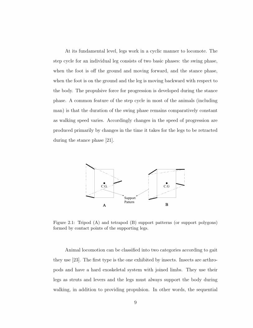
Figure 2.1: Tripod (A) and tetrapod (B) support patterns (or support polygons)formed by contact points of the supporting legs.
Animal locomotion can be classified into two categories according to gait
they use [23]. The first type is the one exhibited by insects. Insects are arthro-
pods and have a hard exoskeletal system with joined limbs. They use their
legs as struts and levers and the legs must always support the body during
walking, in addition to providing propulsion. In other words, the sequential
9
pattern of steps must ensure static stability. The vertical projection of the
center of gravity must therefore always be within the support pattern (the two
dimensional convex polygon formed by the contact points (Fig. 2.1)). This
kind of locomotion has been described as crawling and the legs have to pro-
vide at least tripod of support at all times. Another kind of locomotion may
be observed in humans, horses, dogs, cheetahs, and kangaroos which have a
more flexible structure. These animals require dynamic balance, which is less
stringent restriction on the posture and the gait of the animal. The animal
may not be in static equilibrium. On the contrary, there may be periods of
time when none of the support legs are on the ground as is observed in trotting
horses, running humans, and hopping kangaroos.
The mechanism by which the nervous system generates the cyclic move-
ments of the legs during walking is basically the same in animals [23], [21]. The
first significant efforts analyzing the nervous system were in the beginning of
1900s with the work of two British physiologists, C. S. Sherrington and T.
Graham Brown [21]. Sherrington first showed that rhythmic movements could
be elicited from the hind legs of cats and dogs some weeks after their spinal
cord had been severed. Since the operation had isolated from the rest, the
nervous center that control the movement of the hind legs, he showed that the
higher levels of the nervous system are not necessary for the organization of
stepping movements. He explained the generation of rhythmic leg movements
by a series of ”chain reflexes” (a reflex being a stereotyped movement elicited
by the stimulation of a specific group of sensory receptors). Thus he conceived
that the sensory input generated during any part of the step cycle elicit the
10
next part of the cycle by a reflex action, producing in turn another sensory sig-
nal that elicits the next part of the cycle, and so on. Whereas, Graham Brown
demonstrated that rhythmic contractions of leg muscles, similar to those that
occur during walking, could be induced immediately following transection of
the spinal cord even in animals in which all input from sensory nerves in the
legs had been eliminated. So, Graham claimed that mechanisms located en-
tirely within the spinal cord are responsible for generating the basic rhythm
for stepping in each leg.
Actually these two concepts are not compatible but neither provides a
complete explanation by itself [21]. Further experiments in a number of labo-
ratories have yielded results that strongly support the dual view of the nervous
mechanisms involved in walking. Both approaches have attractive features as
models for understanding how neural systems produce behavior. If walking is
the consequence of complete motions (central pattern), then it is much easier
to see how phase coordination of multiple legs is possible. On the other hand,
it is more difficult to see how adaptation to details of the terrain is possible
when walking is composed of complete motions. This state of affairs is re-
versed when the model is based on reflexes. The consensus that evolved was
that aspects of both models are important to the control of locomotion and
that neither was completely correct by itself [21]. Thus, our gait synthesizer
joins both sensory effects, environmental task performance as reinforcement
and simple neural structure for phase coordination of the multiple legs of our
robot. However our generated system is reflexive enough to adapt to the sud-
den unevenness of the terrain in rescue operations.
11
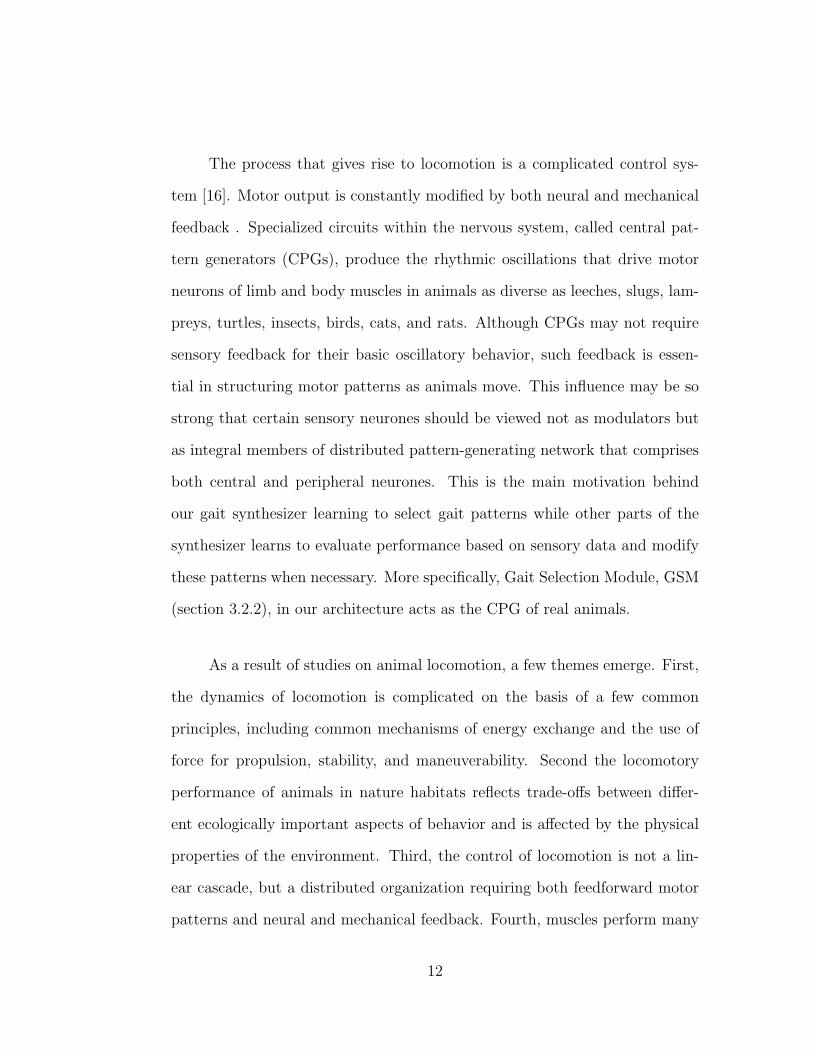
The process that gives rise to locomotion is a complicated control sys-
tem [16]. Motor output is constantly modified by both neural and mechanical
feedback . Specialized circuits within the nervous system, called central pat-
tern generators (CPGs), produce the rhythmic oscillations that drive motor
neurons of limb and body muscles in animals as diverse as leeches, slugs, lam-
preys, turtles, insects, birds, cats, and rats. Although CPGs may not require
sensory feedback for their basic oscillatory behavior, such feedback is essen-
tial in structuring motor patterns as animals move. This influence may be so
strong that certain sensory neurones should be viewed not as modulators but
as integral members of distributed pattern-generating network that comprises
both central and peripheral neurones. This is the main motivation behind
our gait synthesizer learning to select gait patterns while other parts of the
synthesizer learns to evaluate performance based on sensory data and modify
these patterns when necessary. More specifically, Gait Selection Module, GSM
(section 3.2.2), in our architecture acts as the CPG of real animals.
As a result of studies on animal locomotion, a few themes emerge. First,
the dynamics of locomotion is complicated on the basis of a few common
principles, including common mechanisms of energy exchange and the use of
force for propulsion, stability, and maneuverability. Second the locomotory
performance of animals in nature habitats reflects trade-offs between differ-
ent ecologically important aspects of behavior and is affected by the physical
properties of the environment. Third, the control of locomotion is not a lin-
ear cascade, but a distributed organization requiring both feedforward motor
patterns and neural and mechanical feedback. Fourth, muscles perform many
12
different functions in locomotion, a view expanded by the integration of muscle
physiology with whole-animal mechanics (muscles can act as motors, brakes,
springs, and struts).
Because machines face the same physical laws and environmental con-
straints that biological systems face when they perform similar tasks, the solu-
tions they use may embrace similar principles. Legged machines have a lot of
things to learn from the nature. But, evolutionary pressures that dictate the
morphology and physiology of animals do not always give the suitable results
for our tasks. For example, % 40 of the body mass of a shrimp is devoted to the
large, tasty abdominal muscles that produce a powerful tail flick during rare,
but critical, escape behaviors [16]. The imitation of a such body design will
surely result in an inefficient machine. The consequence is that the informa-
tion taken from the nature must be processed and the fundamental principles
must be defined. That is why we concentrated on redundant legged robots
and more specifically 6 legged ones.
2.2.2 Control of Legged Robots
The main challenge for legged robots is the control system. A system
that controls such a robot accomplishes several tasks [5]. First it regulates the
robot’s gait, that is, the sequence and way in which the legs share the task
of locomotion. For example, six legged robots work with gaits that elevate a
single leg at a time or two or three legs simultaneously. A gait that elevates
several legs at once generally makes it possible to travel faster but offers less
stability than a gait that keeps more legs on the ground.
13
A second task is to keep the robot from tipping over. For the vehicles
using static stability, if the center of gravity of the robot moves beyond the
base of support provided by the legs, the robot will tip. So, location of the
center of gravity with respect to the placement of the feet must be continuously
monitored by the robot. In our control structure, static stability is provided
by ensuring safety margins from physical limits such as the distance of the
center of gravity from the support polygon and distance of the legs from their
reaching limits during support phase.
Since many legs share the support of the body, a third task is to dis-
tribute the support load and the lateral forces among the legs. Smoothness of
the ride and minimal disturbance of the ground are the main objectives during
this task. In this thesis work the smoothness of the legged robot is provided
by applying periodic wave gait patterns of the insects. The perturbations of
the ground to the robot are compensated by choosing proper gaits during the
locomotion.
A fourth task is to make sure the legs are not driven past the limits
during their travel. The geometry of the legs may make it possible for one leg
to bump into another. Control system must take into account the limits of
the leg’s motion and the expected motion of the robot during that leg’s stance
period. In our robot the legs’ operation areas are restricted such that they do
not overlap.
A fifth task is to choose places for stepping that will give adequate sup-
14
port. For this task a sensor system that would scan the ground ahead of the
robot will be required. This system will build an internal digital model of the
terrain and process to find suitable footholds. Here, softness of the terrain may
cause problems. In the gait synthesizer we developed, a task oriented internal
model is learned during the learning process of gait evaluation.
We perform these five tasks (which are related to locomotion) on a hexa-
pod robot by focusing on gait control. In other words, our solutions to the
problems in the overall control of the hexapod robot are based on gait con-
trol. For the rest of the tasks which depend on the application, we just show
the potential of the gait synthesizer. Specifically, we will show that the gait
synthesizer is capable of adapting to the rescue operations where a leg of the
hexapod is used as manipulator while the rest provide mobility. However, the
key challenge in legged robots is to control individual components (legs) for
cooperative manipulation, while obtaining their cooperation for walking as an
integrated whole. This is behind the motivation of this thesis work.
2.2.3 Gait Analysis
In this thesis we focus on gaits of legged robots. A gait is a sequence
of leg motions coordinated with a sequence of body motions for the purpose
of transporting the body of the legged system from one place to another [8].
Gait analysis is one of the fundamental areas in the study of walking robots.
It is important because it is the major factor that affects the geometric and
control design of a walking robot [30]. In general, there are two types of gaits:
periodic and non-periodic gaits [8].
15
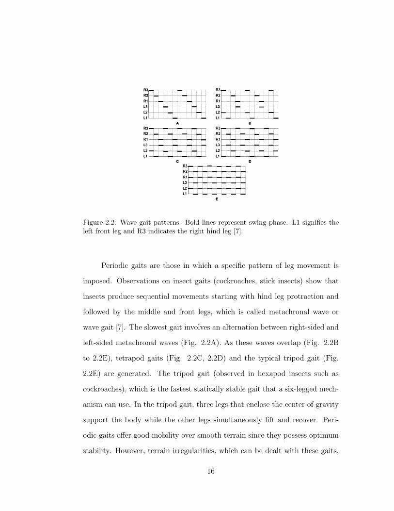
Figure 2.2: Wave gait patterns. Bold lines represent swing phase. L1 signifies theleft front leg and R3 indicates the right hind leg [7].
Periodic gaits are those in which a specific pattern of leg movement is
imposed. Observations on insect gaits (cockroaches, stick insects) show that
insects produce sequential movements starting with hind leg protraction and
followed by the middle and front legs, which is called metachronal wave or
wave gait [7]. The slowest gait involves an alternation between right-sided and
left-sided metachronal waves (Fig. 2.2A). As these waves overlap (Fig. 2.2B
to 2.2E), tetrapod gaits (Fig. 2.2C, 2.2D) and the typical tripod gait (Fig.
2.2E) are generated. The tripod gait (observed in hexapod insects such as
cockroaches), which is the fastest statically stable gait that a six-legged mech-
anism can use. In the tripod gait, three legs that enclose the center of gravity
support the body while the other legs simultaneously lift and recover. Peri-
odic gaits offer good mobility over smooth terrain since they possess optimum
stability. However, terrain irregularities, which can be dealt with these gaits,
16
are relatively limited. If the terrain irregularity is severe such as in natural
disaster areas, periodic gaits become ineffective, and special gates need to be
developed. These gaits are non-periodic gaits. Works in this area comprise of
studies on free gaits [32], and large obstacle gaits [30]. Free gaits are gaits in
which any leg is permitted to move at any time [31]. In free gait approach, a
finite set of gait states is defined and control is done on a rule-based principle,
resulting in simple motions lack of smoothness. Our gait control approach
takes the advantages of these gaits in order to achieve a smooth and adaptive
locomotion over unpredictive terrain roughness.
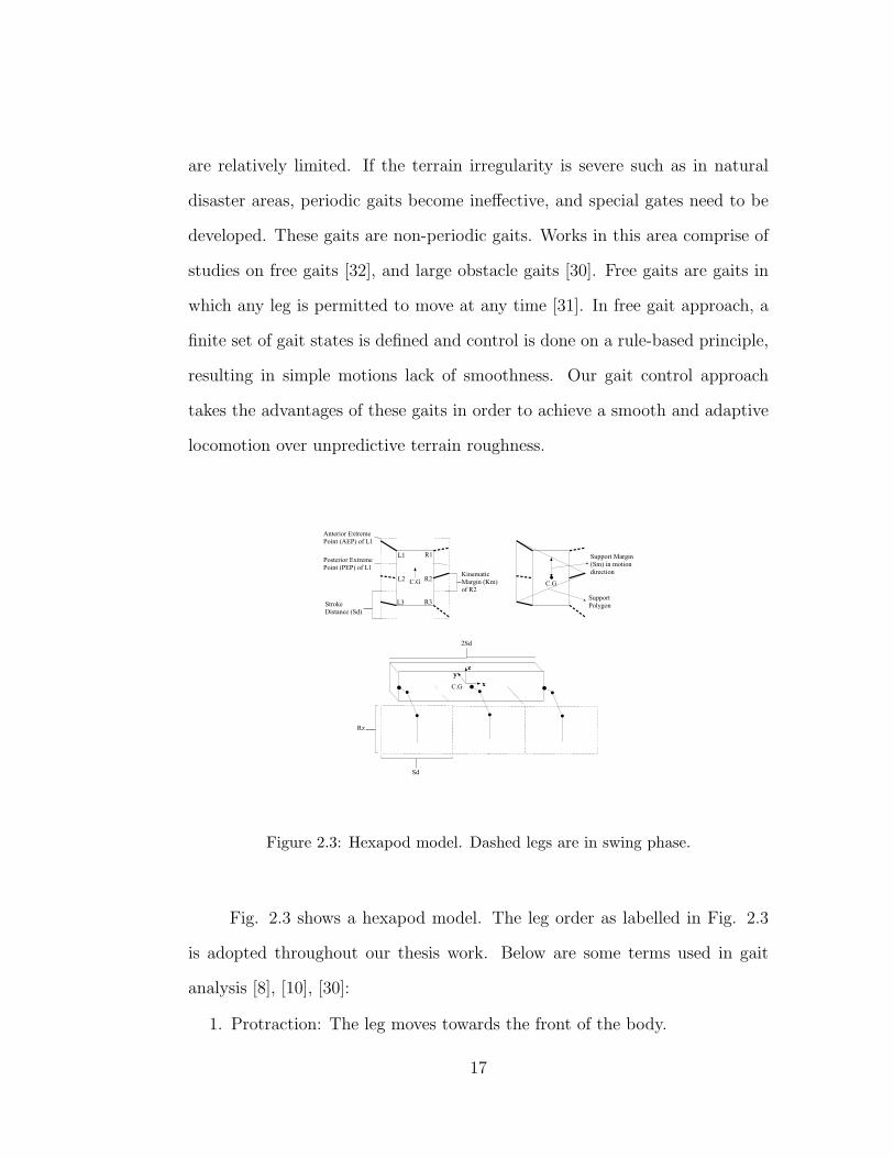
Figure 2.3: Hexapod model. Dashed legs are in swing phase.
Fig. 2.3 shows a hexapod model. The leg order as labelled in Fig. 2.3
is adopted throughout our thesis work. Below are some terms used in gait
analysis [8], [10], [30]:
1. Protraction: The leg moves towards the front of the body.
17
2. Retraction: The leg moves towards the rear of the body.
3. Stance phase: The leg is on the ground where it supports and propels
the body. In forward walking, the leg retracts during this phase. Also
called power stroke or support phase.
4. Swing phase: The leg lifts and swings to the starting position of the next
stance phase. In forward walking, the leg protracts during this phase.
Also called the return stroke or recovery phase.
5. Cycle time: The time for a complete cycle of leg locomotion of a periodic
gait.
6. Duty factor of a leg: The time fraction of a cycle time in which the leg
is in the support phase.
7. Phase of a leg: The fraction of a cycle period by which the current leg
position follows the placement of the leg.
8. Support Polygon: Two dimensional point set in a horizontal plane con-
sisting of the convex hull of the vertical projection of all foot points in
support phase (Fig. 2.3).
9. Stability Margin (Sm): The shortest distance of the vertical projection
of center of gravity to the boundaries of the support pattern in the hor-
izontal plane.
10. Front and Rear Boundary: The boundaries of the support polygon, re-
spectively ahead of and behind the projection of center of gravity in
forward walking, and intersect the longitudinal body axis.
18
11. Front and Rear Stability Margin (Front and Rear Sm): The distances
from the vertical projection of the center of gravity to the front and rear
boundaries of the support polygon respectively, in forward walking.
12. Kinematic Margin (Sm): The distance from the current foothold of a
stance leg to the border of its reachable area in the opposite direction of
body motion (Fig. 2.3).
13. Anterior Extreme Position (AEP): In forward walking, this is the target
position of the advance degree of freedom during recovery phase. It is
the foremost position a leg reaches during a cycle.
14. Posterior Extreme Position (PEP): In forward walking, this is the target
position of the swing degree of freedom during support phase. It is the
backmost position a leg reaches during a cycle.
15. The Stroke distance (Sd): The distance between Anterior Extreme Point
(AEP) and Posterior Extreme Point (PEP).
2.2.4 Gait Control
One of the aspects related with the control of legged robots is the genera-
tion of stable gaits [31]. The task of gait generation mechanism can be defined
as selecting an appropriate coordination sequence of leg and body movements
so that the robot advances with a desired speed and direction. Gait generation
for six legged (or more) robots has been addressed with several researches that
we will overview here.
19
The principle stated by experimental studies of walking in insects is that
gaits arise from the interaction of individual leg oscillators (step pattern gen-
erators) which govern the stepping of each leg by exchanging the influences
of the legs [9]. The information transmitted from the step pattern generator
depends upon the leg’s state (either swing or stance, position and velocity).
Here the position information plays a particular central role in coordination.
We take this also into consideration in our work.
Several versions of this interleg coordination principle is investigated and
implemented in insect-inspired walking robots. Pearson [21] proposed that
modification of the walking coordination may occur through load sensors in
the leg’s chordotonal organ and position information from the campaniform
sensillae. This model formed the basis of Beer’s simulation of cockroach be-
haviors [18] where the effect of load and position sensors was simulated by
forward and backward angle sensor ”neurons” as well as ground contact and
stance and swing ”neurons” within a distributed neural network control archi-
tecture. This basic model was then implemented on a walking robot with two
degrees of freedom per leg [19].
A more complex interleg coordination model is proposed by [20] and
[24]. Together they identify at least six mechanisms that work between legs in
a stick insect. A summary of the coordination mechanisms in the stick insect is
shown in Fig. 2.4. The arrows indicate the direction of influences which estab-
lish the coordination of the legs providing stability. In [24], [25] most of these
mechanisms are simulated and some of them have also been implemented on a
robot with two dof per leg [26] and two robots with three dof per leg [27]. In
20
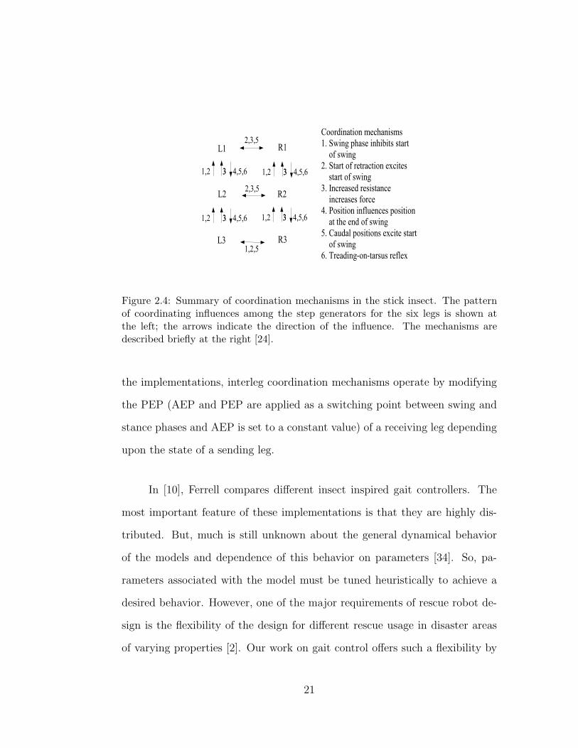
Figure 2.4: Summary of coordination mechanisms in the stick insect. The patternof coordinating influences among the step generators for the six legs is shown atthe left; the arrows indicate the direction of the influence. The mechanisms aredescribed briefly at the right [24].
the implementations, interleg coordination mechanisms operate by modifying
the PEP (AEP and PEP are applied as a switching point between swing and
stance phases and AEP is set to a constant value) of a receiving leg depending
upon the state of a sending leg.
In [10], Ferrell compares different insect inspired gait controllers. The
most important feature of these implementations is that they are highly dis-
tributed. But, much is still unknown about the general dynamical behavior
of the models and dependence of this behavior on parameters [34]. So, pa-
rameters associated with the model must be tuned heuristically to achieve a
desired behavior. However, one of the major requirements of rescue robot de-
sign is the flexibility of the design for different rescue usage in disaster areas
of varying properties [2]. Our work on gait control offers such a flexibility by
21
drawing decisions from insect-inspired gait patterns to the changing needs of
the terrain and that of rescue.
In the literature some of the complete walking robot designs does not
offer remarkable approaches for gait control [37], [11]. They usually apply
fixed gait patterns (especially tripod). But some researches still focus on the
subject. In [30], Choi and Song deal with obstacle-crossing gaits. Their study
is presented on fully automated gaits that can be used to cross four types
of simplified obstacles: grade, ditch, step, and isolated wall. After the type
and dimensions of an obstacle is entered, the system generates a series of pre-
programmed movements that enables a hexapod to cross over the obstacle in
a fully automated mode. Our approach provides obstacle crossing by trying
different gaits rather than imposing pre-programmed movements.
In [36] a gait state definition is presented as a function of the last steps
executed. They identify several classes of gait states and transitions between
them. They show that independently from the initial posture of robot, the
robot would be in one of the four situations according to the number of legs
in contact by executing a sequence of gait states and the tripod gait can be
obtained.
Yang and Kim focus on the robustness to damages to legs in walking ma-
chines and deal with fault tolerant gaits [28]. These are the gaits maintaining
stability in static walking against a fault event preventing a leg from having
the support state. In [29], they successfully implement a fault tolerant gait
over uneven terrain. In our gait control approach we do not distinguish the
22
gaits according to their fault tolerances but we enable the controller to search
for the gait that will solve the problem.
In [6], Celaya and Porta present a complete control structure for the lo-
comotion of a legged robot on uneven terrain. In the gait generation they use
two rules by which different gaits including the complete family of wave gaits
can be obtained with a proper initial state. With the first rule that is: ’never
have two neighboring legs raised from the ground at the same time’, static
stability is guaranteed. Whereas the second rule: ’a leg should perform a step
when this is allowed by the first rule and its neighboring legs have stepped
more recently than it has’, forces the alternation of the steps of any pair of
neighboring legs. These two rules are local so that no central synchronization
is required.
In [33], a modified version of Q-learning approach is used for the decen-
tralized control of the Robot Kafka. Each leg, which can be in one of finite
number of states, has its own look-up table and can communicate with the
others. Based on the legs’ states and those, to which they are coupled, actions
are chosen according to these lookup tables. Modified Q-learning approach is
employed to search for a set of actions resulting in successful walking gaits.
Parker and et al utilize Cyclic Genetic Algorithm (CGA) to produce
gaits for a hexapod robot [40]. The approach to generate a gait is to develop
a model capable of representing all states of the robot and use a cyclic genetic
algorithm to train this model to walk forward. CGA is developed as a modi-
fication of the standard Genetic Algorithm. The CGA incorporates time into
23
the chromosome structure by assigning each gene a task to be accomplished
in a set amount of time. Also some portions of the chromosome (tasks) are
repeated creating a cycle. This allows the chromosome to represent a program
that has a start section and an iterative section. In [40] it is shown that with
only minimal a priori knowledge the optimal tripod gait for a hexapod robot
can be produced.
In [11], a survey of different approaches for gait generation can be found.
Among the methods in the literature, our gait synthesizer has an hybrid struc-
ture. Interaction of legs (mutual inhibitions and excitations) in biological sys-
tems results in observed gait patterns. Without implementing the described
interleg mechanisms we work on these patterns so that we make use of biolog-
ical background. Whereas our system enables the flexibility of non-periodic
gaits by allowing any leg to move out of the pattern when needed. In our
approach both the terrain conditions and performance criteria determine the
gait to be applied.
2.3 Mathematical Background
2.3.1 Neural-Fuzzy Controllers
Neural Fuzzy Controllers (NFCs), based on a fusion of ideas from fuzzy
control and neural networks, possess the advantages of both neural networks
(e.g., learning abilities, optimization abilities, and connectionist structures)
and fuzzy control systems (e.g., humanlike IF-THEN rule thinking and ease
of incorporating expert knowledge) [13]. Fuzzy systems and neural networks
24
share the common ability to improve the intelligence of systems working in
an uncertain, imprecise, and noisy environment. The main purpose of neural
fuzzy control system is to apply neural learning techniques to find and tune the
parameters and/or structure of the neuro-fuzzy control systems. Some of the
works in this area are Generalized Approximate Reasoning based Intelligent
Control (GARIC) [12], Fuzzy Adaptive Learning Control Network (FALCON)
[52], Adaptive Neuro Fuzzy Inference System (ANFIS) [53], and Neuro-Fuzzy
Control (NEFCON) [54]. In our work we adopted the GARIC architecture in
order to develop the gait synthesizer for our multilegged robot.
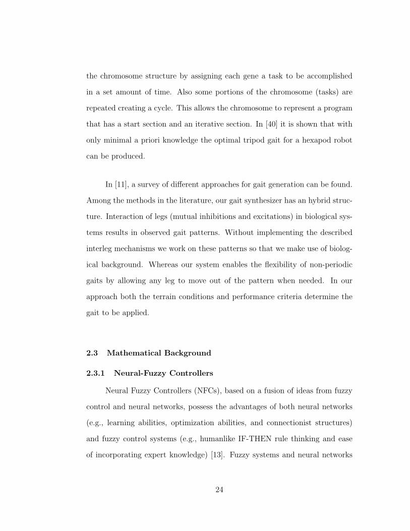
2.3.2 GARIC Architecture
Generalized approximate reasoning-based intelligent control (GARIC),
introduced by Berenji and Khedkar [12], is a neural fuzzy control system with
reinforcement learning capability. GARIC presents a method for learning and
tuning fuzzy logic controllers (FLC) through reinforcements signals. It consists
of three modules (Fig. 2.5): an action evaluation network (AEN) that maps
a state vector and a failure signal into a scalar score (internal reinforcement)
indicating the goodness of the state, an action selection network (ASN) that
maps a state vector into a recommended action using fuzzy inference, and a
stochastic action modifier that produces actual action based on internal re-
inforcement. Learning occurs by fine-tuning the free parameters in the two
networks: in the AEN, the weights are adjusted; in the ASN, the parameters
describing the fuzzy membership functions are changed.
25
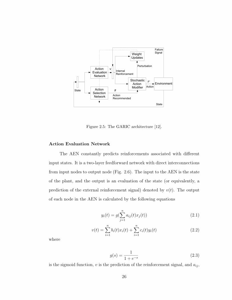
Figure 2.5: The GARIC architecture [12].
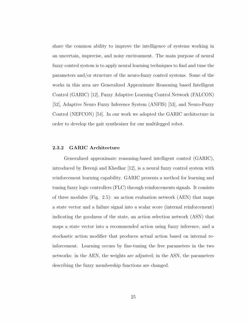
Action Evaluation Network
The AEN constantly predicts reinforcements associated with different
input states. It is a two-layer feedforward network with direct interconnections
from input nodes to output node (Fig. 2.6). The input to the AEN is the state
of the plant, and the output is an evaluation of the state (or equivalently, a
prediction of the external reinforcement signal) denoted by v(t). The output
of each node in the AEN is calculated by the following equations
yi(t) = g(n∑
j=1
aij(t)xj(t)) (2.1)
v(t) =n∑
i=1
bi(t)xi(t) +n∑
i=1
ci(t)yi(t) (2.2)
where
g(s) =1
1 + e−s(2.3)
is the sigmoid function, v is the prediction of the reinforcement signal, and aij,
26
bi, and ci are corresponding link weights shown as A, B, and C in Fig. 2.6.
Figure 2.6: The action evaluation network.
This network evaluates the action recommended by the action network
as a function of the failure signal and the change in state evaluation based on
the state of the system at time t
r(t) =
0 start state
r(t)− v(t− 1) failure state
r(t) + γv(t)− v(t− 1) otherwise
(2.4)
where 0 ≤ γ ≤ 1 is the discount rate. In other words, the change in the value
of v plus the value of the external reinforcement constitutes the heuristic or
internal reinforcement, r, where the future values of v are discounted more the
further they are from the current state of the system.
Learning in AEN is based on internal reinforcement, r(t). If r is positive,
27
the weights are altered so as to increase the output v for positive input, and
vice versa. Therefore, the equations for updating the weights are as follows:
bi(t) = bi(t− 1) + βr(t)xi(t− 1) (2.5)
ci(t) = ci(t− 1) + βr(t)yi(t− 1) (2.6)
aij(t) = aij(t− 1) + βhr(t)yi(t− 1)(1− yi(t− 1))sgn(ci(t− 1))xj(t− 1) (2.7)
where β > 0 and βh > 0 are constant learning rates.
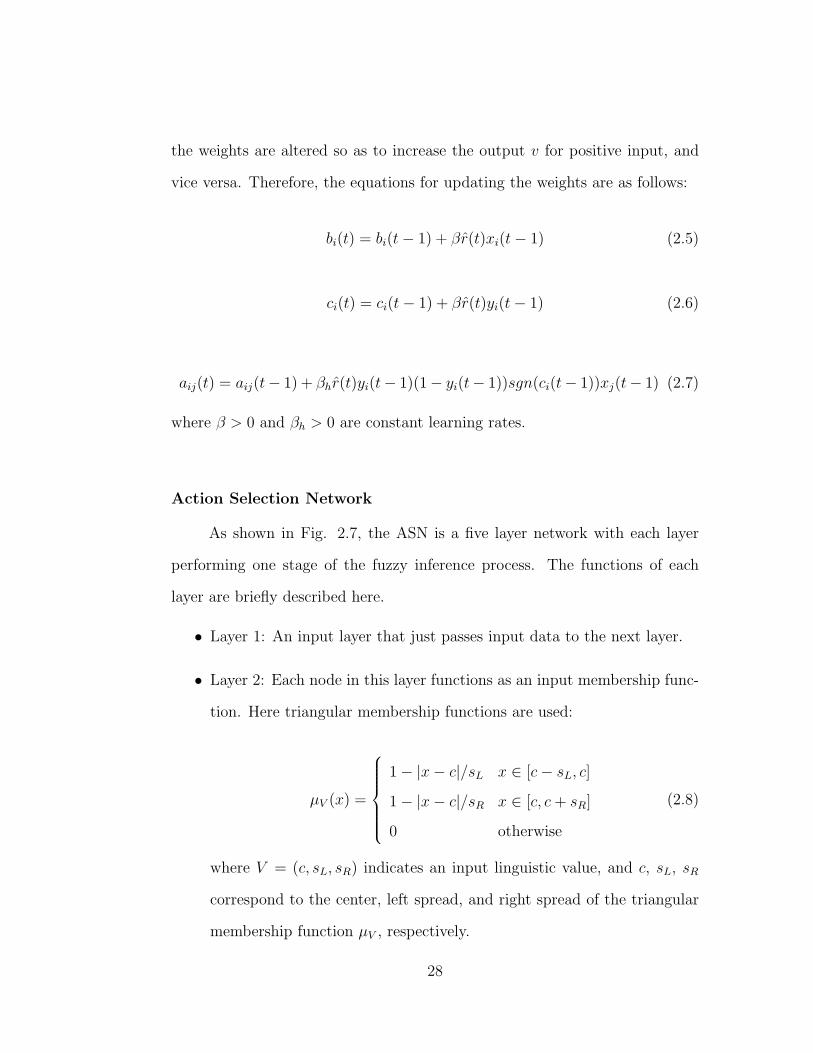
Action Selection Network
As shown in Fig. 2.7, the ASN is a five layer network with each layer
performing one stage of the fuzzy inference process. The functions of each
layer are briefly described here.
• Layer 1: An input layer that just passes input data to the next layer.
• Layer 2: Each node in this layer functions as an input membership func-
tion. Here triangular membership functions are used:
µV (x) =
1− |x− c|/sL x ∈ [c− sL, c]
1− |x− c|/sR x ∈ [c, c + sR]
0 otherwise
(2.8)
where V = (c, sL, sR) indicates an input linguistic value, and c, sL, sR
correspond to the center, left spread, and right spread of the triangular
membership function µV , respectively.
28
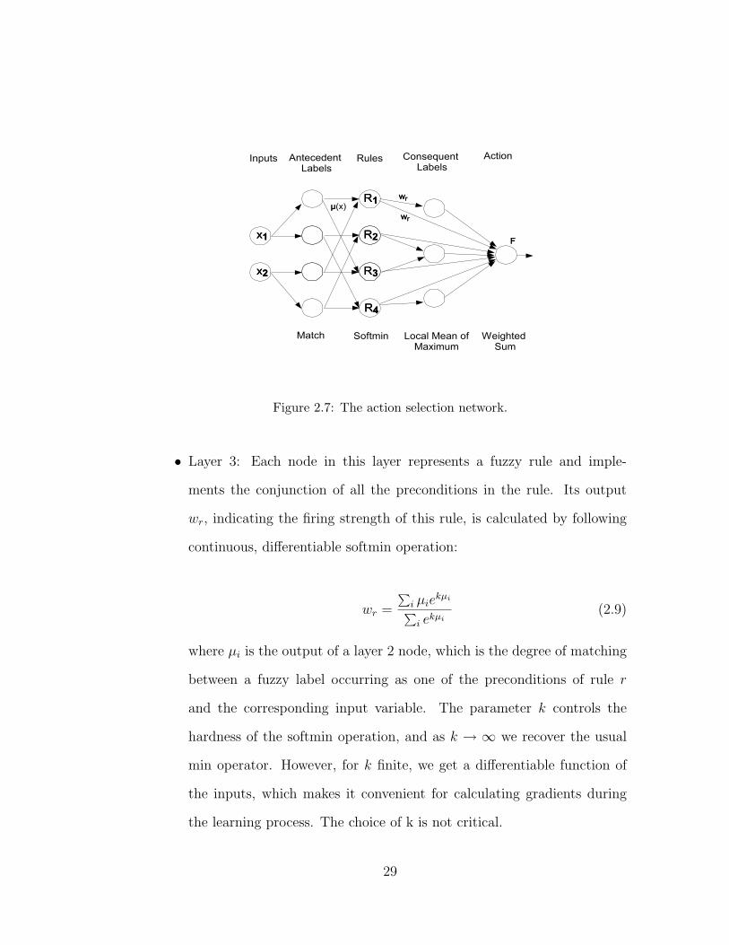
Figure 2.7: The action selection network.
• Layer 3: Each node in this layer represents a fuzzy rule and imple-
ments the conjunction of all the preconditions in the rule. Its output
wr, indicating the firing strength of this rule, is calculated by following
continuous, differentiable softmin operation:
wr =
∑i µie
kµi
∑i ekµi
(2.9)
where µi is the output of a layer 2 node, which is the degree of matching
between a fuzzy label occurring as one of the preconditions of rule r
and the corresponding input variable. The parameter k controls the
hardness of the softmin operation, and as k → ∞ we recover the usual
min operator. However, for k finite, we get a differentiable function of
the inputs, which makes it convenient for calculating gradients during
the learning process. The choice of k is not critical.
29
• Layer 4: Each node in this layer corresponds to a consequent label.
For each of the wr supplied to it, this node computes the corresponding
output action as suggested by rule r. This mapping is written as µ−1(wr),
where the inverse is taken to mean a suitable defuzzification procedure
applicable to an individual rule. For triangular functions,
µ−1Y (wr) = c + 0.5(sR − sL)(1− wr) (2.10)
where Y = (c, sL, sR) indicates a consequent linguistic value.
• Layer 5: Each node in this layer is an output node that combines the
recommendations from all the fuzzy control rules using the following
weighted sum:
F =
∑r wrµ
−1(wr)∑r wr
(2.11)
In the ASN, adjustable weights are present only on the input links of
layers 2 and 4. The other weights are fixed at unity.
Stochastic Action Modifier
In GARIC architecture, the output of ASN is not applied to the environ-
ment directly. Stochastic Action Modifier (SAM) uses the values of r from the
previous time step and the action F recommended by the ASN to stochasti-
cally generate an action, F ′, which is a Gaussian random variable with mean
F and standard deviation σ(r(t − 1)). This σ() is some nonnegative, mono-
tonically decreasing function, e.g. exp(−r). The action F ′ is what is actually
30
applied to the plant. The stochastic perturbation in the suggested action leads
to a better exploration of state space and better generalization ability. When
r(t − 1) is low, meaning the last action performed is bad, the magnitude of
the deviation |F ′ − F | is large, whereas the controller remains consistent with
the fuzzy control rules when r(t− 1) is high. The actual form of the function
σ(), especially its scale and rate of decrease, should take the units and range
of variation of the output variable into account.
In GARIC, the goal of calculating F values in ASN is to maximize
the evaluation of the gait, v, determined by AEN. The gradient information
∆p = δv/δp (p is the vector of all adjustable weights in ASN) is estimated by
stochastic exploration in the Stochastic Action Modifier (SAM). The modifi-
cation implemented in t− 1 by SAM is judged by r(t). If r > 0, meaning the
modified F ′(t − 1) is better than expected, then F (t − 1) is moved closer to
the modified one, and vice versa.
2.3.3 Fuzzy Sets and Fuzzy Logic Controllers
Fuzzy sets, introduced by Zadeh in 1965 as a mathematical way to rep-
resent vagueness in linguistics, can be considered a generalization of classical
set theory [47]. In a classical set, the membership of an element is crisp; it is
either yes (in the set) or no (not in the set). A crisp set can be defined by the
so-called characteristic function (or membership function). The characteristic
function µA(x) of a crisp set A is given as
µA(x) =
1 if x ∈ A
0 if x 6∈ A
31
Fuzzy set theory extends this concept by defining partial memberships,
which can take values ranging from 0 and 1:
µA(x) : U → [0, 1]
where U refers to the universal set defined in a specific problem.
Fuzzy logic was one of the major developments of Fuzzy Set Theory and
was primarily designed to represent and reason with knowledge that cannot
be expressed by quantitative measures. The main idea of algorithms based on
fuzzy logic is to imitate the human reasoning process to control ill-defined or
hard-to-model plants. Fuzzy inference systems model the qualitative aspects
of human knowledge through linguistic if-then rules. Every rule has two parts:
an antecedent part (premise), expressed by if..., which is the description of the
state of the system, and a consequent part, expressed by then..., which is the
action that the operator who controls the system must take.
We can use fuzzy sets to represent linguistic variables. Linguistic vari-
ables represent the process states and control variables in a fuzzy controller.
Their values are defined in linguistic terms and they can be words or sentences
in a natural or artificial language.
The most important operators in classical set theory with crisp sets are
complement, intersection, and union. These operations are defined in fuzzy
logic via membership functions. The membership values in a complement
subset A are
µA(x) = 1− µA(x)
32
which corresponds to the same operation in the classical theory. For the inter-
section of two fuzzy sets various operators have been proposed (min operator,
algebraic product, bounded product,...). The min operator for two fuzzy sets
A and B is given as
µA(x)andµB(x) = min{µA(x), µB(x)}
For the union of two fuzzy sets, there is a class of operators named t-conorms
or s-norms. One of the most used in the literature is the max operator:
µA(x)orµB(x) = max{µA(x), µB(x)}
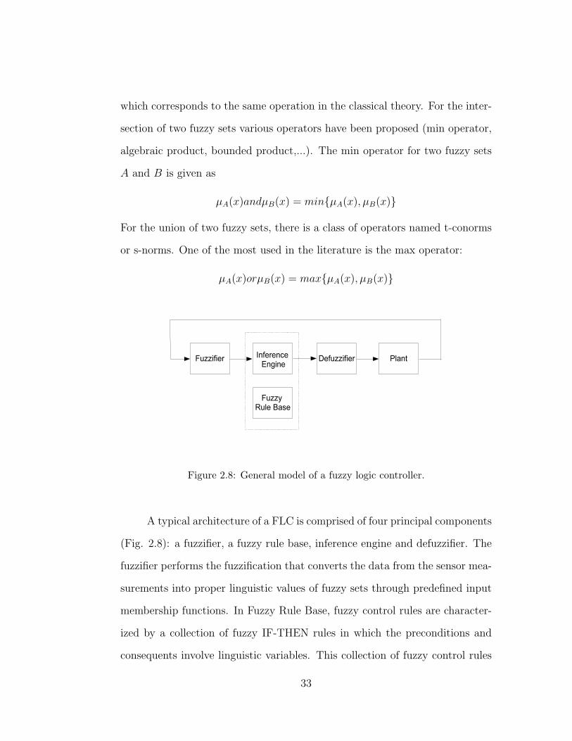
Figure 2.8: General model of a fuzzy logic controller.
A typical architecture of a FLC is comprised of four principal components
(Fig. 2.8): a fuzzifier, a fuzzy rule base, inference engine and defuzzifier. The
fuzzifier performs the fuzzification that converts the data from the sensor mea-
surements into proper linguistic values of fuzzy sets through predefined input
membership functions. In Fuzzy Rule Base, fuzzy control rules are character-
ized by a collection of fuzzy IF-THEN rules in which the preconditions and
consequents involve linguistic variables. This collection of fuzzy control rules
33
(or fuzzy control statements) characterizes the simple input-output relation of
the system. The inference engine is to match the output of the fuzzifier with
the fuzzy logic rules and perform fuzzy implication and approximate reasoning
to decide a fuzzy control action. Finally, the defuzzifier performs the function
of defuzzification to yield a nonfuzzy (crisp) control action from an inferred
fuzzy control action through predefined output membership functions.
The principal elements of designing a FLC include defining input and out-
put variables, deciding on the fuzzy partition of the input and output spaces
and choosing the membership functions for the input and output linguistic
variables, deciding on the types and derivation of fuzzy control rules, design-
ing the inference mechanism, and choosing a defuzzification operator [13].
2.3.4 Reinforcement Learning
Reinforcement learning is an approach to artificial intelligence that em-
phasizes learning by the individual from its interaction with its environment
[13]. The environment supplies a time varying vector of input to the system,
receives its time varying vector of output or action and then provides a time
varying scalar reinforcement signal. Here, the reinforcement signal r(t) can be
one of the following forms: a two valued number r(t) ∈ {-1,1}or {-1,0} such
that r(t)=1 (0) means ”success” and r(t)=-1 means ”failure”; a multi-valued
discrete number in the range [-1,1] or [-1,0], for example r(t) ∈ {-1, -0.5, 0,
0.5, 1}, a real number r(t)=[-1,1] or [-1,0], which represent a more detailed
and continuous degree of failure or success. We also assume that r(t) is the
reinforcement signal available at time step t and is caused by the inputs and
34
actions at time step (t-1) or even affected by earlier inputs and actions.
Challenging problem in reinforcement learning is that there may be a
long time delay between a reinforcement signal and the actions that caused it.
In such cases a temporal credit assignment problem results because we need to
assign credit or blame, for an eventual success or failure, to each step individ-
ually in a long sequence. An approach to solve such problem is based on the
temporal difference methods [41]. TD methods consist of a class of incremental
learning procedures specialized for prediction problems. TD methods assign
credit based on the difference between temporally successive predictions. The
main characteristic of these methods is that it is not required to wait until the
actual outcome is known.
The object of learning is to construct an action selection policy that
optimizes the systems performance. A natural measure of performance is the
discounted cumulative reinforcement (utility [38])
Vt =∞∑
k=0
γkrt+k (2.12)
where Vt is the discounted cumulative reinforcement starting from time t
throughout the future, rt is the reinforcement received after the transition
from time t − 1 to t, and 0 ≤ γ ≤ 1 is a discount factor, which adjusts the
importance of long term consequences of actions. In the approach to solve the
temporal credit assignment problem, the aim is to learn an evaluation func-
tion to predict the discounted cumulative reinforcement. Evaluation function
(V πx ) is the expected discounted cumulative reinforcement that will be received
starting from state x, or simply the utility of state x. The evaluation function
35
is represented using connectionist networks (evaluation network or critic) and
learned using a combination of temporal difference methods and error back-
propagation algorithm. TD methods compute the error called the TD error
between temporally successive predictions, and the backpropagation algorithm
minimizes the error by modifying the weights of the networks.
Let pt is the output of the evaluation network, which denotes the estimate
at time step t for the evaluation function V πx , given the state xt, and rt is the
actual cost incurred between time steps t− 1 and t. Then pt−1 predicts
∞∑
k=0
γkrt+k = rt + γpt (2.13)
In this case the prediction error (TD error) which is the difference between
estimated evaluation and actual evaluation would be
(rt + γpt)− pt−1 (2.14)
This method is used for prediction problems in which exact success or
failure may never become completely known.
36
CHAPTER 3
LEGGED ROBOT
3.1 Dynamics and Coordinated Control of Legged Robots
The dynamics of a robotic system play a central role in both its control
and simulation. When studying the control of robots, the primary problem,
which must be solved, is known as Inverse Dynamics. Solution of the in-
verse dynamics problem requires the calculation of the actuator torques and/or
forces, which will produce a prescribed motion in the robotic system. Whereas,
in the area of simulation, the fundamental problem to be solved is called For-
ward or Direct Dynamics. Solution of this problem requires the determination
of the joint motion, which results from a given set of applied joint torques
and/or forces.
The overall mechanism of a legged robot is a closed-chain comprised of a
body with supporting legs. The kinematic relations between the leg joint mo-
tion and the body motion are complicated. The additional complexity arises
because the chains (legs) of the system are coupled through the body.
In the approach presented here the resemblance between the control of
legged robots and the manipulation of objects by multi-fingered robot hands
is considered. The dynamics and control of grasping are developed in various
prior works [48], [51]. We adapt these concepts here to legged robots. The
basics of the mathematical background given in this section can be found in
[42], [44], [50]. Note that these analysis are valid for legged robots using static
37
balance where the body is continuously supported by at least three legs con-
stituting a support polygon.
The dynamics and control algorithm represented here must be consid-
ered within a complete control system for a legged robot including navigation,
terrain adaptation, etc. Because these concepts are out of the scope of this
thesis work, we will just give the algorithm, however simulations for the gait
synthesizer will be implemented with a simpler model described in chapter 4.
3.1.1 Motion Dynamics of Legged Robots
We firstly derive equations concerned with moving coordinate frames.
Let C1 and C2 be two coordinate frames. We denote by p12 ∈ R3 and R12 ∈SO(3) (3 × 3 orthogonal matrix, R−1 = RT ) the position and orientation of
C2 relative to C1. Beside, we denote by v12 = p12 and w12 = S−1(R12RT12) (or
R12 = S(w12)R12), translational and rotational velocity of C2 relative to C1,
where S is an operator defined by
w =
w1
w2
w3
, S(w) =
0 −w3 w2
w3 0 −w1
−w2 w1 0
which clearly satisfies
S(w)f = w × f and
AS(w)AT = S(Aw) for all A ∈ SO(3), w, f ∈ R3.
Now consider three coordinate frames C1, C2, and C3. The position and
orientation of C3 relative to C1 is given by [50]
38
p13 = p12 + R12p23 (3.1)
R13 = R12R23 (3.2)
Then translational velocity of C3 relative to C1 is obtained by
v13 = p13 = p12 + R12p23 + R12p23 (3.3)
which is
v13 = v12 − S(R12p23)w12 + R12v23 (3.4)
To see this, we observe that
R12p23 = S(w12)R12p23
= (R12RT12)S(w12)R12p23
= R12S(RT12w12)p23
= R12(RT12w12)× p23
= R12(−p23)× (RT12w12)
= −R12S(p23)RT12w12
= −S(R12p23)w12
By differentiating both sides of equation 3.2, we also obtain rotational
velocity of C3 relative to C1:
R13 = R12R23 + R12R23 (3.5)
S(w13)R13 = S(w12)R12R23 + R12S(w23)R23 (3.6)
S(w13)R13 = S(w12)R13 + S(R12w23)R13 (3.7)
w13 = w12 + R12w23 (3.8)
by the transformation
39
R12S(w23)R23 = R12S(w23)(RT12R12)R23
= S(R12w23)R13)
Then the generalized velocity of C3 relative to C1 is given in matrix form
by
v13
w13
=
I −S(R12p23)
0 I
v12
w12
+
R12 0
0 R12
v23
w23
(3.9)
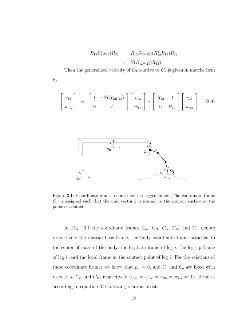
Figure 3.1: Coordinate frames defined for the legged robot. The coordinate frameCci is assigned such that the unit vector z is normal to the contact surface at thepoint of contact.
In Fig. 3.1 the coordinate frames Cw, CB, Cbi, Cti, and Cci denote
respectively the inertial base frame, the body coordinate frame attached to
the center of mass of the body, the leg base frame of leg i, the leg tip frame
of leg i, and the local frame at the contact point of leg i. For the relations of
these coordinate frames we know that ptc = 0, and Cc and Cb are fixed with
respect to Cw and CB, respectively (vwc = wwc = vBb = wBb = 0). Besides,
according to equation 3.9 following relations exist:
40
vbc
wbc
=
I −S(Rbtptc)
0 I
vbt
wbt
+
Rbt 0
0 Rbt
vtc
wtc
=
vbt
wbt
+
Rbt 0
0 Rbt
vtc
wtc
(3.10)
vBc
wBc
=
RBb 0
0 RBb
vbc
wbc
(3.11)
vwc
wwc
=
I −S(RwBpBc)
0 I
vwB
wwB
+
RwB 0
0 RwB
vBc
wBc
= 0
(3.12)
−
I −S(RwBpBc)
0 I
vwB
wwB
=
Rwb 0
0 Rwb
vbc
wbc
(3.13)
−
RTwb −RT
wbS(RwBpBc)
0 RTwb
vwB
wwB
=
vbc
wbc
(3.14)
−T
vwB
wwB
=
vbc
wbc
(3.15)
Moreover, the velocity of leg tip frame, Ct, is related to the velocity of
the leg joints, q, by the leg jacobian,
vbt
wbt
= J(q)q (3.16)
In this analysis, we consider following contact models for the leg tip-
terrain interactions: a) a point contact without friction, b) a point contact
with friction, c) a soft contact, d) a rigid contact. These contact models give
rise to contact constraints specified by
41
• viz = 0, for a point contact without friction.
• vix = vi
y = viz = 0, for a point contact with friction.
• vix = vi
y = viz = 0 and wi
z = 0, for a soft contact.
• vix = vi
y = viz = 0 and wi
x = wiy = wi
z = 0, for a rigid contact.
For each of the contact models, substituting the above contact constraints
and equation 3.16 into equation 3.10 we have
BT
vbc
wbc
= BT J(q)q (3.17)
where BT is the basis matrix defined in [49] representing the model contact
constraints. For example, for a point contact with friction
BT =
1 0 0 0 0 0
0 1 0 0 0 0
0 0 1 0 0 0
(3.18)
Substituting equation 3.17 into equation 3.15 we have
−BT T
vwB
wwB
= BT J(q)q (3.19)
−GT
vwB
wwB
= Jleg(q)q (3.20)
Dual to generalized velocity, a generalized force (or wrench) can be writ-
ten as
F13 =
f13
τ13
(3.21)
42
where τ13 ∈ R3 and f13 ∈ R3 are the torque and the linear force about the
origin of C3 relative to coordinate frame C1, respectively.
Generalized force can be defined by examining the work produced by a
virtual displacement. A virtual displacement is an instantaneous infinitesimal
displacement du. The work produced by a virtual displacement, virtual work,
is denoted by δW , where δW = F · du. We use the principle of virtual work
to find generalized force relations. The work performed, which has units of
energy, must be the same regardless of the coordinate system within which
it is measured or expressed [45]. The virtual work done by an infinitesimal
displacement of the body with respect to Cw is
δW =
fwB
τwB
·
vwB
wwB
=
fwB
τwB
T
vwB
wwB
where we have represented the dot product in the virtual work equation using
the transpose operation. Alternatively, the virtual work done by the corre-
sponding infinitesimal displacement of the Cc with respect to Cb is
δW =
fbc
τbc
·
vbc
wbc
=
fbc
τbc
T
vbc
wbc
By the principle of virtual work, these two formulations of the work performed
are equal:
fwB
τwB
T
vwB
wwB
=
fbc
τbc
T
vbc
wbc
(3.22)
and substituting equation 3.15 into 3.22 we have
fwB
τwB
T
=
fbc
τbc
T
(−T ) (3.23)
43
fwB
τwB
= (−T T )
fbc
τbc
(3.24)
For a given contact model, let ni denote the total number of independent
contact wrenches that leg i can apply to the terrain. For example, ni = 1 for a
point contact without friction (i.e., a force in the normal direction), and ni = 3
for a point contact with friction (i.e., a force in the normal direction plus two
components of frictional forces). Note that ni is just the number of contact
constraints corresponding to the contact model. According to equation 3.24
the resulting generalized force from applied contact force of the leg i can be
expressed as
fwB
τwB
= −T T Bxi (3.25)
fwB
τwB
= −Gxi (3.26)
where xi ∈ Rni is the magnitude vector of applied contact forces (generalized)
along the basis directions of B. Equations 3.20 and 3.26 provide valid relations
if the leg remains in contact with the surface and there is no slipping. A com-
mon way to guarantee no slipping is to ensure that the contact forces lie within
the friction cone at the point of contact-that is, the tangential component of
the contact force is less than or equal to the coefficient of friction µ times the
normal component of the contact force.
Finally for n (i = n) supporting legs
44
Q =
q1
q2
...
qn
FT =
x1
x2
...
xn
JT =[
Jleg1 Jleg2 · · · Jlegn
]
GT =[
G1 G2 · · · Gn
]
Then the equations 3.20 and 3.26 and can be concatenated for i =
1, · · · , n to give,
JT (Q)Q = −GTT
vwB
wwB
(3.27)
−GT FT =
fwB
τwB
(3.28)
We have derived the force,torque and velocity relations from legs to leg-
tips and leg-tips to body.
3.1.2 Coordinated Control of Legged Robots
In this section, we develop the control algorithm for the coordinated
control of the robot legs. The goal of the control scheme is to specify a set of
45
control inputs for the leg motors so that the body undergoes a desired motion.
The control scheme we develop in this section is based on the computed torque
methodology.
By differentiating equation 3.27 we have
JT (Q)Q + JT (Q)Q = −GTT
vwB
wwB
−GT
T
vwB
wwB
(3.29)
Q = J+T (Q)
−GT
T
vwB
wwB
−GT
T
vwB
wwB
− J+
T (Q)JT (Q)Q + Qo
(3.30)
Here J+T (Q) is the pseudo inverse satisfying J+ = JT (JJT )−1 and Qo ∈ N (JT )
is the internal motion of redundant joints not affecting the body motion.
The dynamics of the body expressed in internal base frame Cw is given
by the Newton-Euler equation as [51]
Im 0
0 Iw
vwB
wwB
+
0
wwB × IwwwB
=
fwB
τwB
(3.31)
Here
Im =
mB 0 0
0 mB 0
0 0 mB
where mB is the body mass and Iw = RwBIoRTwB is the body inertia matrix
expressed in Cw and Io is the body inertia matrix expressed in CB. Also from
equation 3.28 we have
46
FT = −G+T
fwB
τwB
+ FTo (3.32)
where G+T is the pseudo inverse of GT and FTo is the internal leg force not
affecting the body motion. Combining equation 3.31 and equation 3.32 yields
FT = −G+T
Im 0
0 Iw
vwB
wwB
+
0
wwB × IwwwB
+ FTo (3.33)
In order to specify an orientation trajectory in terms of the rotation
matrix RwB(t) we parameterize SO(3) so that RwB = RwB(Υ) where Υ ∈ R3
is taken as yaw α(t), pitch β(t), and roll γ(t) coordinates of the body. Given
this parametrization, there exists a linear transformation p(Υ) such that [42]:
w =
wx
wy
wz
=
cγcβ −sγ 0
sγsβ cγ 0
−sβ 0 1
α
β
γ
= p(Υ)Υ (3.34)
where
Υ =
α
β
γ
So the acceleration of the body is given as
vwB
wwB
= P
pwB
ΥwB
+ P
pwB
ΥwB
(3.35)
where
P =
I 0
0 p(Υ)
We define the position error ep ∈ R6 of the body in a given desired
trajectory as
47
ep =
pdwB
ΥdwB
−
pwB
ΥwB
where
pdwB(t)
ΥdwB(t)
is the desired body trajectory.
In order to reduce the position error, we apply joint torques of the legs
to make the acceleration of the body satisfy the equation
vwB
wwB
= P
pdwB
ΥdwB
+ kvep + kpep
+ P
pwB
ΥwB
(3.36)
where kv and kp are scalars chosen such that the characteristic roots of
ep + kvep + kpep = 0 have negative real parts.
The dynamics of the ith leg manipulator for l link is given by
Hi(q)q + Ci(q, q)q = τi − JT (q)Bxi
where
τ = l × 1 vector of joint torques,
q, q, q = l × 1 vectors of joint positions, velocities, and accelerations,
H(q) = l × l joint space inertia matrix , both symmetric and positive definite,
C(q, q) = l × l matrix of coriolis and centripetal force terms,
We define
H =
H1 · · · 0...
. . ....
0 · · · Hn
48
C =
C1
C2
...
Cn
τ =
τ1
τ2
...
τn
Then the leg dynamics can be grouped for i = 1, · · · , n to yield
H(Q)Q + C(Q, Q)Q = τ − JTT (Q)FT (3.37)
Thus the resultant control law is specified by substituting equations 3.30,
3.33, 3.36, 3.37:
τ = DP
pdwB
ΥdwB
+ kvep + kpep
+ DP
pwB
ΥwB
+ E (3.38)
where
D =
−HJ+
T GTT − JT
T G+T
Im 0
0 Iw
and
E = −HJ+T GT
T P
pwB
ΥwB
−HJ+
T JT Q + CQ− JTT G+
T
0
wwB × IwwwB
All the terms in equation 3.38 are functions of state variables Q, Q, pwB,
ΥwB, vwB, and ΥwB.
49
3.2 Gait Controller
Our gait controller is based on a gait synthesizer which is adapted from
the Generalized Approximate Reasoning-based Intelligent Control (GARIC)
architecture [12], to our objective GARIC presents a method for learning and
tuning fuzzy logic controllers (FLC) through reinforcements signals. The gait
synthesizer (Fig. 3.2) consists of three modules. The Gait Evaluation Mod-
ule (GEM), acts as a critic and provides advice to the main controller, based
on a multilayer artificial neural network. The Gait Selection Module (GSM),
decides on a new gait to be undertaken by the robot according to an ANN
representation of a fuzzy controller with as many hidden units as there are
rules in the knowledge base. The Gait Modifier Module (GMM), changes the
gait recommended by the GSM based on internal reinforcement. This change
in the recommended gait is more significant for a state if that state does not
receive high internal reinforcements. (i.e. probability of failure is high). On
the other hand, if a state receives high reinforcements, GMM administers small
changes to the action selected by the fuzzy controller embedded in the GSM.
This reveals that the action is performing well so that the GMM recommen-
dation dictates no or only minor changes to that gait. The actions for the gait
synthesizer are the gaits recommending an operation mode (defined in section
3.3.1) for each leg.
3.2.1 Encoding the Gaits for a Multilegged Robot
Our gait synthesizer works on gait patterns that need to be coded.
Gait patterns are patterns of leg coordination which represents relative phases
50
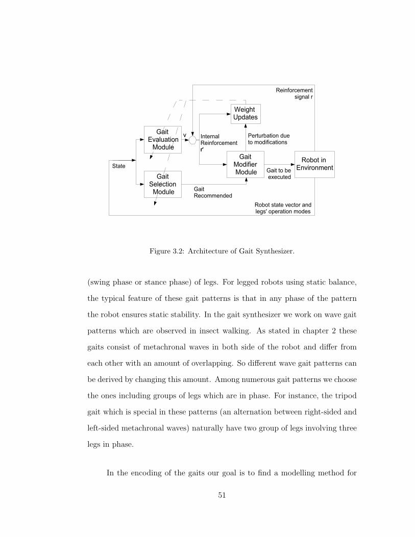
Figure 3.2: Architecture of Gait Synthesizer.
(swing phase or stance phase) of legs. For legged robots using static balance,
the typical feature of these gait patterns is that in any phase of the pattern
the robot ensures static stability. In the gait synthesizer we work on wave gait
patterns which are observed in insect walking. As stated in chapter 2 these
gaits consist of metachronal waves in both side of the robot and differ from
each other with an amount of overlapping. So different wave gait patterns can
be derived by changing this amount. Among numerous gait patterns we choose
the ones including groups of legs which are in phase. For instance, the tripod
gait which is special in these patterns (an alternation between right-sided and
left-sided metachronal waves) naturally have two group of legs involving three
legs in phase.
In the encoding of the gaits our goal is to find a modelling method for
51
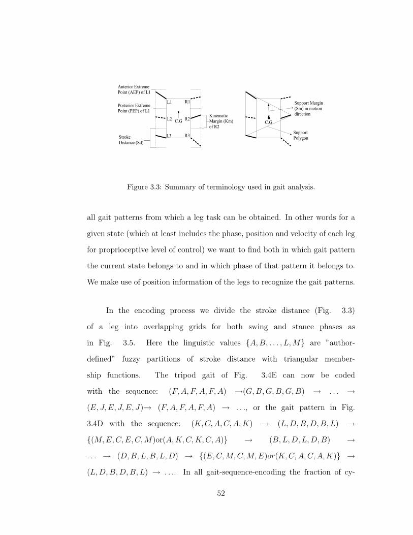
Figure 3.3: Summary of terminology used in gait analysis.
all gait patterns from which a leg task can be obtained. In other words for a
given state (which at least includes the phase, position and velocity of each leg
for proprioceptive level of control) we want to find both in which gait pattern
the current state belongs to and in which phase of that pattern it belongs to.
We make use of position information of the legs to recognize the gait patterns.
In the encoding process we divide the stroke distance (Fig. 3.3)
of a leg into overlapping grids for both swing and stance phases as
in Fig. 3.5. Here the linguistic values {A,B, . . . , L,M} are ”author-
defined” fuzzy partitions of stroke distance with triangular member-
ship functions. The tripod gait of Fig. 3.4E can now be coded
with the sequence: (F, A, F, A, F, A) →(G,B, G, B, G,B) → . . . →(E, J,E, J, E, J)→ (F, A, F, A, F,A) → . . ., or the gait pattern in Fig.
3.4D with the sequence: (K, C, A,C, A,K) → (L,D, B, D, B, L) →{(M, E, C, E,C,M)or(A,K,C,K, C, A)} → (B,L, D, L, D, B) →. . . → (D, B, L,B, L, D) → {(E,C, M,C,M, E)or(K,C,A, C, A, K)} →(L,D, B, D, B, L) → . . .. In all gait-sequence-encoding the fraction of cy-
52
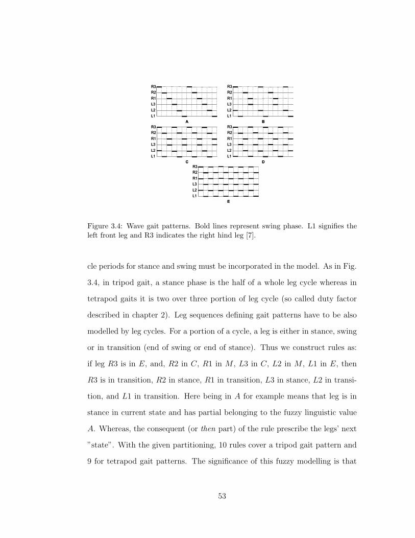
Figure 3.4: Wave gait patterns. Bold lines represent swing phase. L1 signifies theleft front leg and R3 indicates the right hind leg [7].
cle periods for stance and swing must be incorporated in the model. As in Fig.
3.4, in tripod gait, a stance phase is the half of a whole leg cycle whereas in
tetrapod gaits it is two over three portion of leg cycle (so called duty factor
described in chapter 2). Leg sequences defining gait patterns have to be also
modelled by leg cycles. For a portion of a cycle, a leg is either in stance, swing
or in transition (end of swing or end of stance). Thus we construct rules as:
if leg R3 is in E, and, R2 in C, R1 in M , L3 in C, L2 in M , L1 in E, then
R3 is in transition, R2 in stance, R1 in transition, L3 in stance, L2 in transi-
tion, and L1 in transition. Here being in A for example means that leg is in
stance in current state and has partial belonging to the fuzzy linguistic value
A. Whereas, the consequent (or then part) of the rule prescribe the legs’ next
”state”. With the given partitioning, 10 rules cover a tripod gait pattern and
9 for tetrapod gait patterns. The significance of this fuzzy modelling is that
53
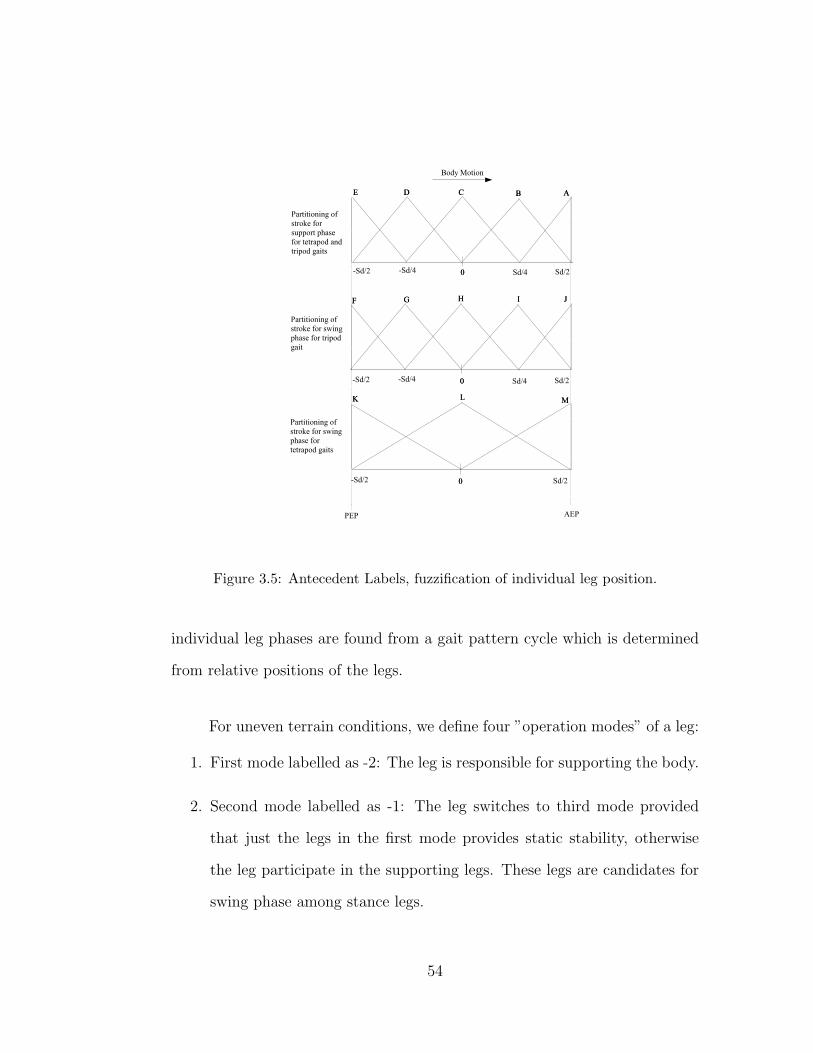
Figure 3.5: Antecedent Labels, fuzzification of individual leg position.
individual leg phases are found from a gait pattern cycle which is determined
from relative positions of the legs.
For uneven terrain conditions, we define four ”operation modes” of a leg:
1. First mode labelled as -2: The leg is responsible for supporting the body.
2. Second mode labelled as -1: The leg switches to third mode provided
that just the legs in the first mode provides static stability, otherwise
the leg participate in the supporting legs. These legs are candidates for
swing phase among stance legs.
54
3. Third mode labelled as 2: The leg is responsible for full recovery such as
that if it encounters an obstacle it will try to handle it.
4. Fourth mode labelled as 1: The leg tip will descend to the ground until
the tip touches the terrain and switches to the first mode.
In both mode labels 2 and 1 (modes will be mentioned with their labels from
now on), the leg will go on recovery if it is within the limits of its operation
space. These four modes constitute leg states from control point of view that
we need to distinguish for a leg within the cooperative action of walking. At
Anterior Extreme Point (AEP), mode 2 automatically switches to mode 1.
Furthermore, the binary data from static stability check for mode -2 legs and
tip contact (a protracting leg switches to retraction when it finds a foothold
that it can safely support the body) clearly determine the switching from mode
-1 to mode 2 and from mode 1 to mode -2, respectively.
Beside the leg/leg coordination, leg/body coordination is required for a
regular gait. Movement of each leg can be characterized by a position p ∈ R
and a velocity p ∈ {vstance(vst), vswing(vsw)} according to direction of body mo-
tion in leg centered coordinates. When a leg is in protraction, it is lifted from
the ground and swing forward relative to the body with a constant velocity
vsw > 0. When a leg is in retraction, it is on the ground, providing support and
swinging backward relative to the body with a velocity vst < 0 (for straight
line walking this velocity is equal to minus body velocity with respect to the
ground, vB). As in many walking animals, vsw is relatively constant while
vst varies according to walking speed. In other words considering Fig 3.4, the
body or retraction velocity is a fraction of protraction velocity and the fraction
55
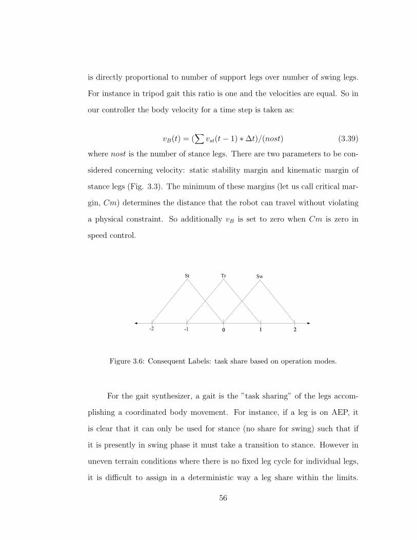
is directly proportional to number of support legs over number of swing legs.
For instance in tripod gait this ratio is one and the velocities are equal. So in
our controller the body velocity for a time step is taken as:
vB(t) = (∑
vst(t− 1) ∗∆t)/(nost) (3.39)
where nost is the number of stance legs. There are two parameters to be con-
sidered concerning velocity: static stability margin and kinematic margin of
stance legs (Fig. 3.3). The minimum of these margins (let us call critical mar-
gin, Cm) determines the distance that the robot can travel without violating
a physical constraint. So additionally vB is set to zero when Cm is zero in
speed control.
Figure 3.6: Consequent Labels: task share based on operation modes.
For the gait synthesizer, a gait is the ”task sharing” of the legs accom-
plishing a coordinated body movement. For instance, if a leg is on AEP, it
is clear that it can only be used for stance (no share for swing) such that if
it is presently in swing phase it must take a transition to stance. However in
uneven terrain conditions where there is no fixed leg cycle for individual legs,
it is difficult to assign in a deterministic way a leg share within the limits.
56
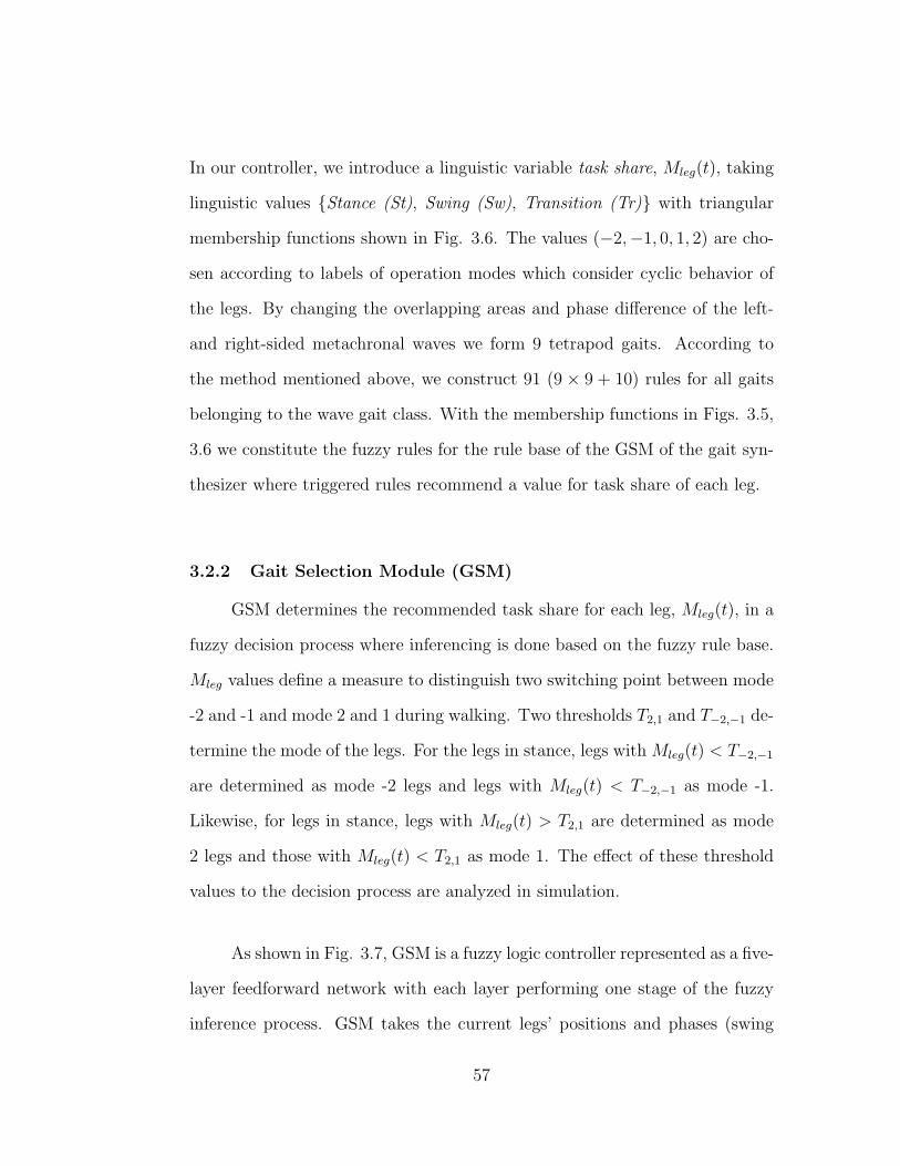
In our controller, we introduce a linguistic variable task share, Mleg(t), taking
linguistic values {Stance (St), Swing (Sw), Transition (Tr)} with triangular
membership functions shown in Fig. 3.6. The values (−2,−1, 0, 1, 2) are cho-
sen according to labels of operation modes which consider cyclic behavior of
the legs. By changing the overlapping areas and phase difference of the left-
and right-sided metachronal waves we form 9 tetrapod gaits. According to
the method mentioned above, we construct 91 (9 × 9 + 10) rules for all gaits
belonging to the wave gait class. With the membership functions in Figs. 3.5,
3.6 we constitute the fuzzy rules for the rule base of the GSM of the gait syn-
thesizer where triggered rules recommend a value for task share of each leg.
3.2.2 Gait Selection Module (GSM)
GSM determines the recommended task share for each leg, Mleg(t), in a
fuzzy decision process where inferencing is done based on the fuzzy rule base.
Mleg values define a measure to distinguish two switching point between mode
-2 and -1 and mode 2 and 1 during walking. Two thresholds T2,1 and T−2,−1 de-
termine the mode of the legs. For the legs in stance, legs with Mleg(t) < T−2,−1
are determined as mode -2 legs and legs with Mleg(t) < T−2,−1 as mode -1.
Likewise, for legs in stance, legs with Mleg(t) > T2,1 are determined as mode
2 legs and those with Mleg(t) < T2,1 as mode 1. The effect of these threshold
values to the decision process are analyzed in simulation.
As shown in Fig. 3.7, GSM is a fuzzy logic controller represented as a five-
layer feedforward network with each layer performing one stage of the fuzzy
inference process. GSM takes the current legs’ positions and phases (swing
57
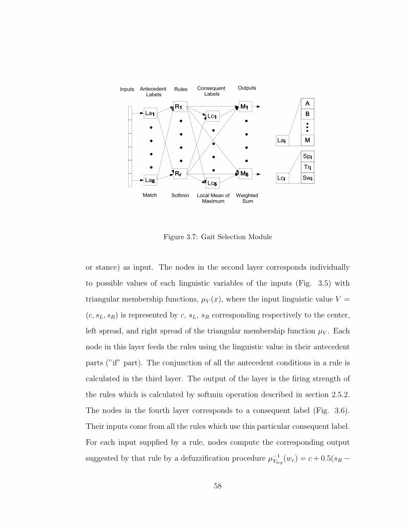
Figure 3.7: Gait Selection Module
or stance) as input. The nodes in the second layer corresponds individually
to possible values of each linguistic variables of the inputs (Fig. 3.5) with
triangular membership functions, µV (x), where the input linguistic value V =
(c, sL, sR) is represented by c, sL, sR corresponding respectively to the center,
left spread, and right spread of the triangular membership function µV . Each
node in this layer feeds the rules using the linguistic value in their antecedent
parts (”if” part). The conjunction of all the antecedent conditions in a rule is
calculated in the third layer. The output of the layer is the firing strength of
the rules which is calculated by softmin operation described in section 2.5.2.
The nodes in the fourth layer corresponds to a consequent label (Fig. 3.6).
Their inputs come from all the rules which use this particular consequent label.
For each input supplied by a rule, nodes compute the corresponding output
suggested by that rule by a defuzzification procedure µ−1Yleg
(wr) = c + 0.5(sR −
58
sL)(1 − wr) where Yleg = (c, sL, sR) indicates a consequent linguistic value of
a leg. In the last layer there are six output node for each leg that computes
Mleg(t) by combining the recommendations from all the fuzzy control rules in
the rule base, using weighted sum in which the weights are the rule strengths:
Mleg = (∑r
wrµ−1(wr))/
∑r
wr (3.40)
The goal of calculating Mleg values in GSN is to maximize the evaluation
of the gait, v, determined by GEM where, within its learning process the vector
of all parameters of Yleg (centers and spreads) are adjusted; that is,
∆pY ∝ δv
δpY
(3.41)
where pY is the vector of Yleg = (c, sL, sR). But, there is no explicit gradi-
ent information provided by the reinforcement signal and the gradient δv/δp
can only be estimated. To estimate the gradient information in reinforcement
learning, there needs to be some randomness in how output gaits are chosen
by GSM so that the range of possible outputs can be explored to find a correct
value. This is provided by the stochastic exploration in Gait Modifier Module
(GMM).
3.2.3 Gait Evaluation Module (GEM)
GEM is a standard two-layer feedforward neural network, which takes
the state of the system as input. The state data includes leg-tip positions,
and velocities in leg centered coordinate systems and legs’ operation mode
(-2,-1,1,2). To assign credit to the individual actions of the action sequence
preceding a reinforcement signal, an evaluation function of the states is learned.
59
The output is an evaluation of the state denoted by v. Changes in v due to
state transitions are further combined with a reinforcement signal to produce
an internal reinforcement r:
r(t) = r(t) + γv(t)− v(t− 1) (3.42)
where 0 ≤ γ ≤ 1 is the discount rate. The internal reinforcement plays the role
of an error measure in the learning of the GEM. If r is positive, the weights of
the network are altered through back propagation algorithm so as to increase
the output v for positive input, and vice versa. The main reinforcement signal
is obtained from critical margin (Cm) and vB. If Cm = 0 or vB = 0 (may
be zero if there are no legs in swing) a reinforcement signal r(t) = −1 is re-
turned. Otherwise a value is returned according to design goal. This value
can be simply r(t) = 0 or can be a real number to represent a more detailed
and continuous degree of success. Different reinforcement signals are tested in
simulations in order to optimize speed and mobility.
3.2.4 Gait Modifier Module (GMM)
One of the features of the Gait Synthesizer architecture is to modify the
output of the GSM according to internal reinforcement from previous time
steps. GMM creates a Gaussian random distribution with a mean which is set
as the recommended Mleg value, and with a standard deviation αexp(−r(t−1)),
a non negative, monotonically decreasing function with a scale factor α, where
α ∈ R+. When r(t − 1) is low, meaning the last action performed is bad,
the deviation is large, whereas the controller remains consistent with the fuzzy
control rules when r(t − 1) is high. This deviation provides adaptation to
60

current conditions or to solving a sudden problem of leg entrapment. Also
the exploration of the state space increases the systems experience, which is
provided by the learning in the GEM and GSM. The gradient information
∆pY = δv/δpY , which is within GSM, is estimated by stochastic exploration
in the GMM. The modification implemented in t − 1 by GMM is judged by
r(t). If r > 0, meaning the modified M(t − 1) is better than expected, then
M(t− 1) is moved closer to the modified one, and vice versa. That is,
δv
δpY
≈ r(t)
[Mmod(t− 1)−Mrec(t− 1)
αexp(−r(t− 1))
](3.43)
where Mrec denotes the M value recommended by GSM, and Mmod denotes
the M value modified by stochastic perturbation in GMM.
Due to change in Mleg values, four different transitions may occur: If a
leg’s state is -2 (-1) and Mleg(t) > T−2,−1 (Mleg(t) < T−2,−1) then leg is -1 (-2).
If a leg’s state is 2 (1) and Mleg(t) < T2,1 (Mleg(t) > T2,1) then leg is 1 (2).
So stochastic exploration on Mleg values which does not result in a modified
transition, have no contribution in learning. We can define the minimum
deviation, ∆dm, as the minimum perturbation added by GMM required to
change the state of a leg. ∆dm(t) values can be given as
∆dm(t) =
|Mrec(t)− T2,1| if the leg is in state 2 or 1
|Mrec(t)− T−2,−1| if the leg is in state -2 or -1
So the modification of an M(t) depends on the deviation function and
the ∆dm(t). The effect of the values α, T2,1, and T−2,−1 will be analyzed in
simulations.
61
3.2.5 The Complete Control Cycle
The control cycle in Fig. 3.8 is executed in each time step. Firstly, re-
inforcement signal and legs’ states are taken by the gait synthesizer and the
legs are clustered to suitable operation modes according to their calculated M
values. Then, further modifications depending on physical checks are applied
and the resultant operation modes which will be valid for the rest of control
layers are obtained until the next cycle. In the figure we only consider velocity
controller, but different control modules (such as navigation, terrain adapta-
tion) can be implemented. Lastly, desired velocities of the legs and the body
is calculated and applied by the robot.
62
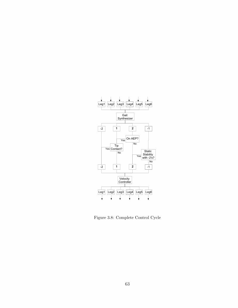
Figure 3.8: Complete Control Cycle
63
CHAPTER 4
HEXAPOD ROBOT SIMULATION
We develop the hexapod robot shown in Fig. 4.1 to be used in our sim-
ulations. Our simulation program consists of two subprograms. The first one
constitutes the main body (main program) which includes the controller ar-
chitecture and the hexapod model. All simulation tests and training sessions
are implemented in this subprogram which is written in Matlab 6.5. The sec-
ond subprogram is responsible for visualization (rendering) of the simulation
results. The main program saves as a file named simvars.bsd the state data
of the hexapod for each time cycle. The state data are fed as an input to the
rendering program. The rendering program is written in Borland C Builder
with opengl as a graphics tool. The reason for using two separate program in
the simulation is to decrease the computation time spent in the tests of the
hexapod. The source code of the programs and simulation results can be found
in the CD attached to this thesis as an appendix.
4.1 Hexapod Model
The simulations are implemented in a kinematic model. Such kinematic
models are commonly implemented in gait analysis [24], [34] and gait control
[30], [28] for simulation purposes. A simplified model of the hexapod robot
considered in this thesis is shown in Fig. 4.2. Each leg is identical and com-
posed of three rigid links (Fig. 4.3). All the links are connected to each other
via a revolute joint. Hence the foot point or the leg tip has three degrees of
64
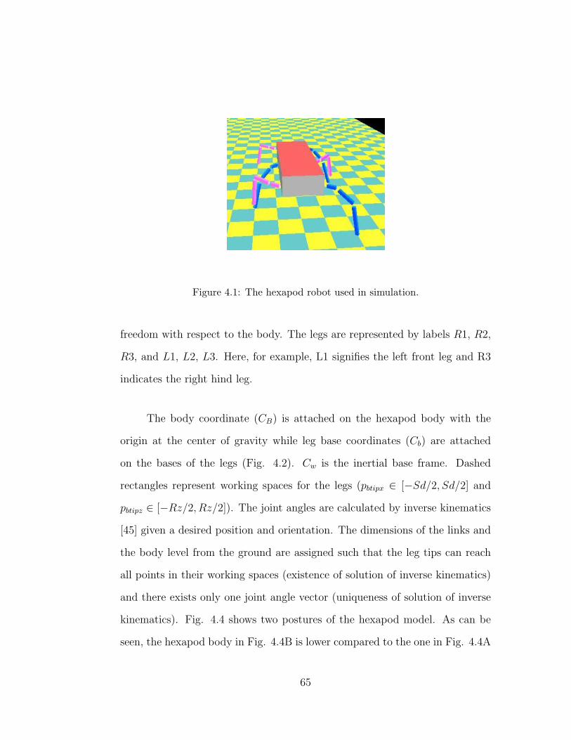
Figure 4.1: The hexapod robot used in simulation.
freedom with respect to the body. The legs are represented by labels R1, R2,
R3, and L1, L2, L3. Here, for example, L1 signifies the left front leg and R3
indicates the right hind leg.
The body coordinate (CB) is attached on the hexapod body with the
origin at the center of gravity while leg base coordinates (Cb) are attached
on the bases of the legs (Fig. 4.2). Cw is the inertial base frame. Dashed
rectangles represent working spaces for the legs (pbtipx ∈ [−Sd/2, Sd/2] and
pbtipz ∈ [−Rz/2, Rz/2]). The joint angles are calculated by inverse kinematics
[45] given a desired position and orientation. The dimensions of the links and
the body level from the ground are assigned such that the leg tips can reach
all points in their working spaces (existence of solution of inverse kinematics)
and there exists only one joint angle vector (uniqueness of solution of inverse
kinematics). Fig. 4.4 shows two postures of the hexapod model. As can be
seen, the hexapod body in Fig. 4.4B is lower compared to the one in Fig. 4.4A
65
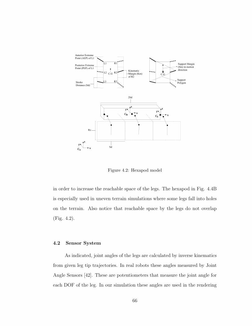
Figure 4.2: Hexapod model
in order to increase the reachable space of the legs. The hexapod in Fig. 4.4B
is especially used in uneven terrain simulations where some legs fall into holes
on the terrain. Also notice that reachable space by the legs do not overlap
(Fig. 4.2).
4.2 Sensor System
As indicated, joint angles of the legs are calculated by inverse kinematics
from given leg tip trajectories. In real robots these angles measured by Joint
Angle Sensors [42]. These are potentiometers that measure the joint angle for
each DOF of the leg. In our simulation these angles are used in the rendering
66
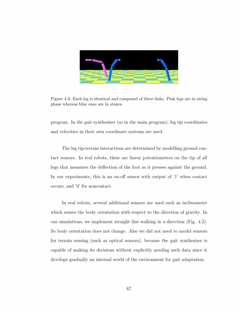
Figure 4.3: Each leg is identical and composed of three links. Pink legs are in swingphase whereas blue ones are in stance.
program. In the gait synthesizer (so in the main program), leg tip coordinates
and velocities in their own coordinate systems are used.
The leg tip-terrain interactions are determined by modelling ground con-
tact sensors. In real robots, these are linear potentiometers on the tip of all
legs that measures the deflection of the foot as it presses against the ground.
In our experiments, this is an on-off sensor with output of ’1’ when contact
occurs, and ’0’ for noncontact.
In real robots, several additional sensors are used such as inclinometer
which senses the body orientation with respect to the direction of gravity. In
our simulations, we implement straight line walking in x-direction (Fig. 4.2).
So body orientation does not change. Also we did not need to model sensors
for terrain sensing (such as optical sensors), because the gait synthesizer is
capable of making its decisions without explicitly needing such data since it
develops gradually an internal world of the environment for gait adaptation.
67
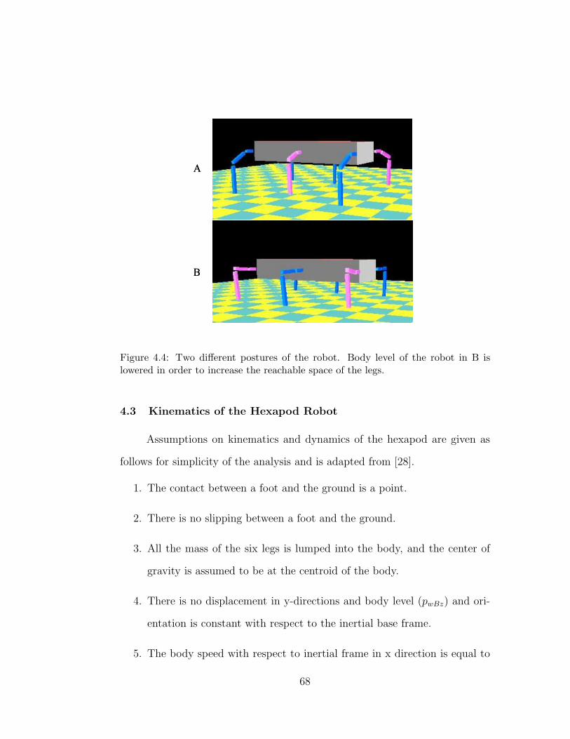
Figure 4.4: Two different postures of the robot. Body level of the robot in B islowered in order to increase the reachable space of the legs.
4.3 Kinematics of the Hexapod Robot
Assumptions on kinematics and dynamics of the hexapod are given as
follows for simplicity of the analysis and is adapted from [28].
1. The contact between a foot and the ground is a point.
2. There is no slipping between a foot and the ground.
3. All the mass of the six legs is lumped into the body, and the center of
gravity is assumed to be at the centroid of the body.
4. There is no displacement in y-directions and body level (pwBz) and ori-
entation is constant with respect to the inertial base frame.
5. The body speed with respect to inertial frame in x direction is equal to
68
minus leg tip speed in x direction of stance legs with respect to Cb(i.e.,
vwBx = −vbtipstx).
In our simulations vbtipswx is set to a constant positive value ρ from which
vwBx (so vbtipstx) is calculated. Also |vbtipswz| = % for swinging legs. For different
states (operation modes) the velocities of the legs are calculated as follows.
vbtipx =
ρ if the leg is in state 2 or 1 and pbtipx(t− 1) < Sd/2 (AEP)
0 if the leg is in state 2 or 1 and pbtipx(t− 1) > Sd/2 (AEP)
ν if the leg is in state −2 or −1
(4.1)
where ν = (∑
vbtipswx(t− 1)∆t)/(nost) and nost is the number of stance legs.
And
vbtipz =
% if the leg is in state 2 and pbtipx(t− 1) <(Rz/2)
−% if the leg is in state 1 and pbtipx(t− 1) >(-Rz/2)
0 otherwise
(4.2)
4.4 Uneven Terrain
The main challenge of the gait synthesizer is for uneven terrain locomo-
tion. The test path for uneven terrain is modelled such that a smooth surface
succeeding a part with randomly placed hills and holes, some of which are
deeper than the legs can reach (Fig. 4.5). A function in the main program
named as TTerrainmaker.m (refer to the CD in the appendix) creates terrains
by randomly placing 7 different surface segments which have dimensions such
69
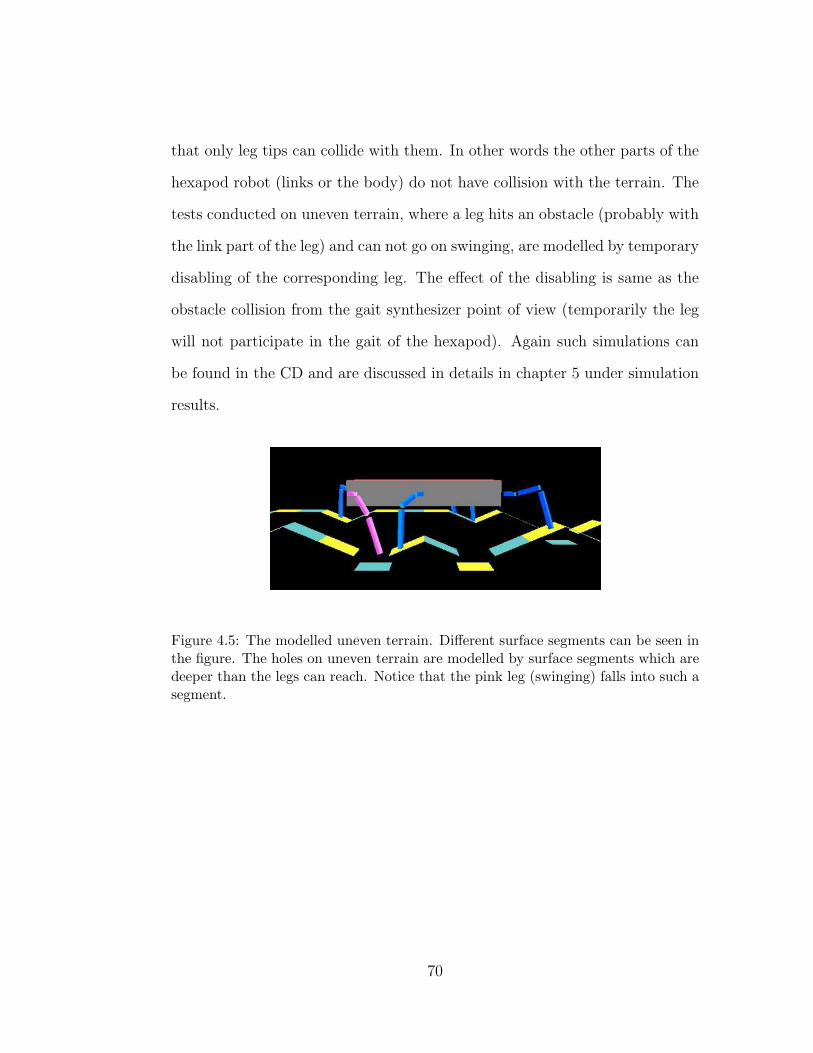
that only leg tips can collide with them. In other words the other parts of the
hexapod robot (links or the body) do not have collision with the terrain. The
tests conducted on uneven terrain, where a leg hits an obstacle (probably with
the link part of the leg) and can not go on swinging, are modelled by temporary
disabling of the corresponding leg. The effect of the disabling is same as the
obstacle collision from the gait synthesizer point of view (temporarily the leg
will not participate in the gait of the hexapod). Again such simulations can
be found in the CD and are discussed in details in chapter 5 under simulation
results.
Figure 4.5: The modelled uneven terrain. Different surface segments can be seen inthe figure. The holes on uneven terrain are modelled by surface segments which aredeeper than the legs can reach. Notice that the pink leg (swinging) falls into such asegment.
70
CHAPTER 5
SIMULATION RESULTS
The hexapod robot simulation developed in chapter 4 is used to gen-
erate simulation results that clearly demonstrate the capabilities of our gait
synthesizer. The simulations are implemented in a kinematic model (chapter
4) rather than the dynamic model described in chapter 3.1. A control system
in such a dynamic model has to include many control modules besides a gait
controller, such as control algorithms related to navigation, speed, body level
(terrain adaptation), which have only effects on the low level execution of a
gait of the robot rather than to the gait formulation level. Consequently the
simulation omits these effects and analyze just the gait synthesizer in the gait
control of a hexapod robot based on its kinematic model.
In the first two sections of the simulations we will firstly analyze the con-
trol parameters and different choice of reinforcement signals that are significant
in the performance of the gait synthesizer. These tests will be implemented
on smooth terrains in order to focus on comparisons under similar environ-
mental effects. In the rest of the simulations we will show the capabilities of
the gait synthesizer for search and rescue (SAR) by testing its performance on
modelled uneven terrains expected in SAR operations and when a leg is used
as a manipulator. Before these tests are implemented, the gait synthesizer
was trained with different initial conditions and with different terrains (for the
tests applied on uneven terrain). The results presented here are chosen among
the ones which are impressive enough to clearly demonstrate the advantages
71
of the gait synthesizer and the potential it offers for SAR. All the results are
included in a CD which is attached to the thesis as an appendix. The reader
is referred to this CD in which the results discussed here can be examined
visually.
5.1 Exploration and Exploitation Dilemma in Reinforcement
Learning
As indicated in the Gait Modifier Module (GMM) the deviation func-
tion αexp(−r(t− 1)) is scaled by α, and two threshold values, T−2,−1 and T2,1
must be properly selected for the controller. The effects of these values are
tested first for a simple learning problem. The legs begin from random initial
positions (all the legs are in state −2) such that this initial configuration does
not belong to any gait pattern in the fuzzy rule base. Since the reinforcement
signals aim at optimizing the speed of the hexapod with a maximized static
stability, we expect that from this random initialization the gait will converge
to the optimum one in terms of speed which is the tripod gait. In order to test
the sensitivity of the gait synthesizer to changes in α and thresholds we test
the GSM in the same manner for each α and threshold values. Within each
training session, repeated 10 times maximum, the gait synthesizer is trained
for 2000 time steps for a given parameter set (α, T2,1, and T−2,−1). We ini-
tialize the weights in learning, change the parameters and apply the training
again for a new parameter set. Fig. 5.1 shows the resultant speed vs time
graphs of the hexapod. In the first test the parameters are chosen as; α = 0.5,
T2,1 = 0.5, and T−2,−1 = −0.5. If the magnitude of the scale factor (α) is
72
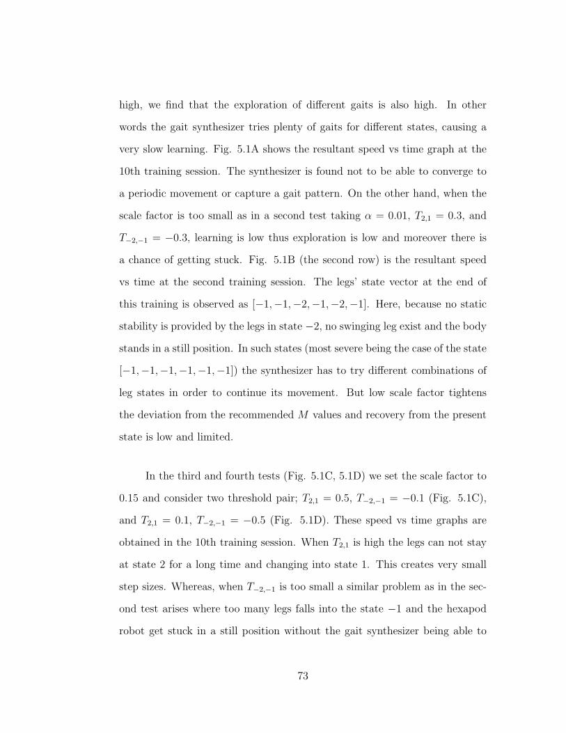
high, we find that the exploration of different gaits is also high. In other
words the gait synthesizer tries plenty of gaits for different states, causing a
very slow learning. Fig. 5.1A shows the resultant speed vs time graph at the
10th training session. The synthesizer is found not to be able to converge to
a periodic movement or capture a gait pattern. On the other hand, when the
scale factor is too small as in a second test taking α = 0.01, T2,1 = 0.3, and
T−2,−1 = −0.3, learning is low thus exploration is low and moreover there is
a chance of getting stuck. Fig. 5.1B (the second row) is the resultant speed
vs time at the second training session. The legs’ state vector at the end of
this training is observed as [−1,−1,−2,−1,−2,−1]. Here, because no static
stability is provided by the legs in state −2, no swinging leg exist and the body
stands in a still position. In such states (most severe being the case of the state
[−1,−1,−1,−1,−1,−1]) the synthesizer has to try different combinations of
leg states in order to continue its movement. But low scale factor tightens
the deviation from the recommended M values and recovery from the present
state is low and limited.
In the third and fourth tests (Fig. 5.1C, 5.1D) we set the scale factor to
0.15 and consider two threshold pair; T2,1 = 0.5, T−2,−1 = −0.1 (Fig. 5.1C),
and T2,1 = 0.1, T−2,−1 = −0.5 (Fig. 5.1D). These speed vs time graphs are
obtained in the 10th training session. When T2,1 is high the legs can not stay
at state 2 for a long time and changing into state 1. This creates very small
step sizes. Whereas, when T−2,−1 is too small a similar problem as in the sec-
ond test arises where too many legs falls into the state −1 and the hexapod
robot get stuck in a still position without the gait synthesizer being able to
73
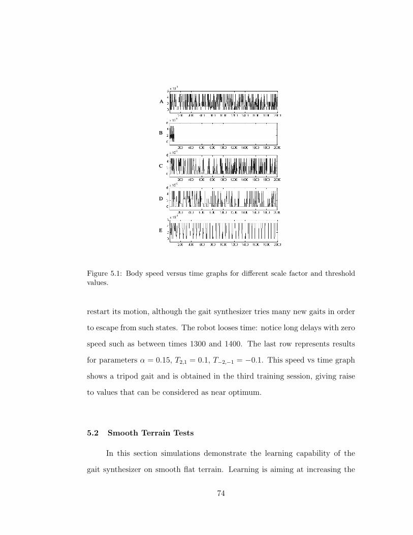
Figure 5.1: Body speed versus time graphs for different scale factor and thresholdvalues.
restart its motion, although the gait synthesizer tries many new gaits in order
to escape from such states. The robot looses time: notice long delays with zero
speed such as between times 1300 and 1400. The last row represents results
for parameters α = 0.15, T2,1 = 0.1, T−2,−1 = −0.1. This speed vs time graph
shows a tripod gait and is obtained in the third training session, giving raise
to values that can be considered as near optimum.
5.2 Smooth Terrain Tests
In this section simulations demonstrate the learning capability of the
gait synthesizer on smooth flat terrain. Learning is aiming at increasing the
74
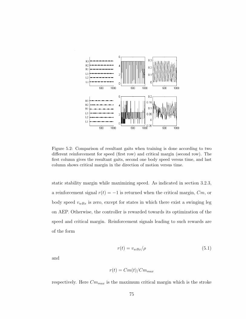
Figure 5.2: Comparison of resultant gaits when training is done according to twodifferent reinforcement for speed (first row) and critical margin (second row). Thefirst column gives the resultant gaits, second one body speed versus time, and lastcolumn shows critical margin in the direction of motion versus time.
static stability margin while maximizing speed. As indicated in section 3.2.3,
a reinforcement signal r(t) = −1 is returned when the critical margin, Cm, or
body speed vwBx is zero, except for states in which there exist a swinging leg
on AEP. Otherwise, the controller is rewarded towards its optimization of the
speed and critical margin. Reinforcement signals leading to such rewards are
of the form
r(t) = vwBx/ρ (5.1)
and
r(t) = Cm(t)/Cmmax
respectively. Here Cmmax is the maximum critical margin which is the stroke
75
distance (Sd), and ρ is the maximum speed of the body according to the speed
policy which can be obtained in tripod gait. The first row of Fig. 5.2 shows the
results of speed optimized gait. The first column gives the resultant gait, sec-
ond one vwBx versus time and last column shows critical margin versus time in
the direction of motion. As expected a tripod gait is obtained because it is the
fastest gait in the rule base of the gait synthesizer and this is where naturally
gait decision has converged to. Maximum speed in second column corresponds
to ρ. The results in the second row corresponds to the gait synthesizer trained
to optimize Cm. As can be seen, a tetrapod gait is obtained which generates
steps to prevent the critical margin from getting smaller (graph in the third
column of second row). The drawback here is on the speed as seen in the
second column.
0 500 1000 1500 2000 2500−1.5
−1
−0.5
0
0.5
1
Figure 5.3: Internal reinforcement versus time.
Another example demonstrates a compromise the gait synthesizer under-
goes in its performance in the case of a tripod gait with small step sizes. The
76
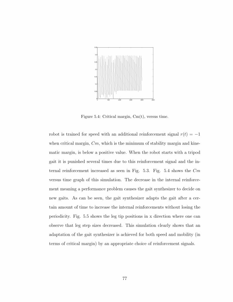
0 500 1000 1500 2000 25000
0.05
0.1
0.15
0.2
0.25
0.3
0.35
Figure 5.4: Critical margin, Cm(t), versus time.
robot is trained for speed with an additional reinforcement signal r(t) = −1
when critical margin, Cm, which is the minimum of stability margin and kine-
matic margin, is below a positive value. When the robot starts with a tripod
gait it is punished several times due to this reinforcement signal and the in-
ternal reinforcement increased as seen in Fig. 5.3. Fig. 5.4 shows the Cm
versus time graph of this simulation. The decrease in the internal reinforce-
ment meaning a performance problem causes the gait synthesizer to decide on
new gaits. As can be seen, the gait synthesizer adapts the gait after a cer-
tain amount of time to increase the internal reinforcements without losing the
periodicity. Fig. 5.5 shows the leg tip positions in x direction where one can
observe that leg step sizes decreased. This simulation clearly shows that an
adaptation of the gait synthesizer is achieved for both speed and mobility (in
terms of critical margin) by an appropriate choice of reinforcement signals.
77
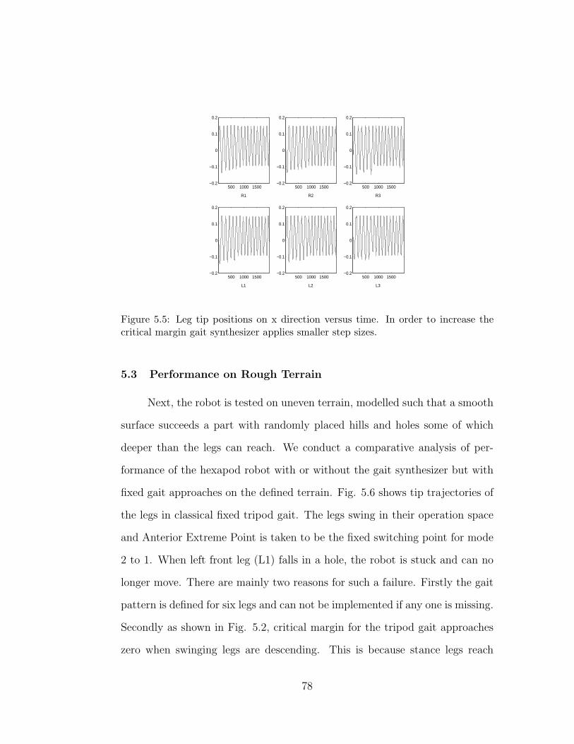
500 1000 1500−0.2
−0.1
0
0.1
0.2
R1
500 1000 1500−0.2
−0.1
0
0.1
0.2
R2
500 1000 1500−0.2
−0.1
0
0.1
0.2
R3
500 1000 1500−0.2
−0.1
0
0.1
0.2
L1
500 1000 1500−0.2
−0.1
0
0.1
0.2
L2
500 1000 1500−0.2
−0.1
0
0.1
0.2
L3
Figure 5.5: Leg tip positions on x direction versus time. In order to increase thecritical margin gait synthesizer applies smaller step sizes.
5.3 Performance on Rough Terrain
Next, the robot is tested on uneven terrain, modelled such that a smooth
surface succeeds a part with randomly placed hills and holes some of which
deeper than the legs can reach. We conduct a comparative analysis of per-
formance of the hexapod robot with or without the gait synthesizer but with
fixed gait approaches on the defined terrain. Fig. 5.6 shows tip trajectories of
the legs in classical fixed tripod gait. The legs swing in their operation space
and Anterior Extreme Point is taken to be the fixed switching point for mode
2 to 1. When left front leg (L1) falls in a hole, the robot is stuck and can no
longer move. There are mainly two reasons for such a failure. Firstly the gait
pattern is defined for six legs and can not be implemented if any one is missing.
Secondly as shown in Fig. 5.2, critical margin for the tripod gait approaches
zero when swinging legs are descending. This is because stance legs reach
78
Posterior Extreme Point (PEP) so there exist no margin for body movement
to handle the hole. Fig. 5.7 shows tip trajectories and Fig. 5.8 shows the
resultant gait when gait synthesizer is implemented on the same terrain. The
gait synthesizer successfully handles the terrain irregularities. When the robot
first enters the uneven portion of the terrain, the evaluation of the gait give
lower reinforcements (due to unexpected bad performance in the robot state)
and new gaits are recommended by the gait synthesizer. When a leg falls in
a hole the synthesizer generates very small steps as ripples in the trajectories.
These hesitations are actually trials of new gaits by Gait Modifier Module and
are also seen on the trajectories of the legs’ tips while they are swinging. One
can argue that a different fixed gait (for instance a tetrapod gait) can tackle
such terrain. This is true from mobility point of view. However for search and
rescue tasks, speed (or response time) is as important as mobility and a fixed
tetrapod gait has a slower performance quite inadequate for a time pressing
SAR operation. Compromise is needed between two concepts. Fig. 5.8 also
shows that after some time the robot reaches the smooth terrain where it re-
covers a tripod gait. Gait trials for a better evaluation of the gait can be seen
from these results where recoveries occur. The results of an another example
for a similar terrain is given in Fig. 5.9, 5.10, and 5.11 where a faster recovery
of the tripod gait is achieved.
5.4 Task Shapability: A Must for SAR Operations
In search and rescue (SAR) operations a leg of the hexapod can be re-
quired to be used for tasks such as carrying debris or any equipment while
79
the robot is in motion, so that it can not participate in the gait of the hexa-
pod. Such a task shapability may be vital in hazardous environment of SAR.
Fig. 5.12 and 5.13 represent such a situation where leg R1 is involved in a
manipulation task and is eliminated from the gait pattern. The leg involved
in a manipulation task is shown here as fixed in a position in swing phase as
if it is holding something. Although the gait synthesizer is seen not being able
to find right away a periodic gait, it provides the mobility in sudden lack of
a leg using the redundancy in multi-legged locomotion. Simulations clearly
indicate the advantageous characteristics of the gait synthesizer for mobility
and robustness required in search and rescue (refer to CD in the appendix).
80
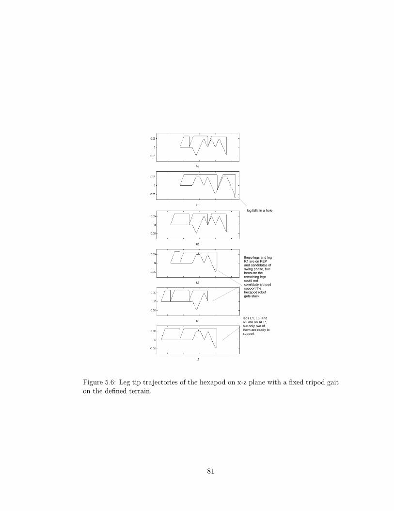
Figure 5.6: Leg tip trajectories of the hexapod on x-z plane with a fixed tripod gaiton the defined terrain.
81
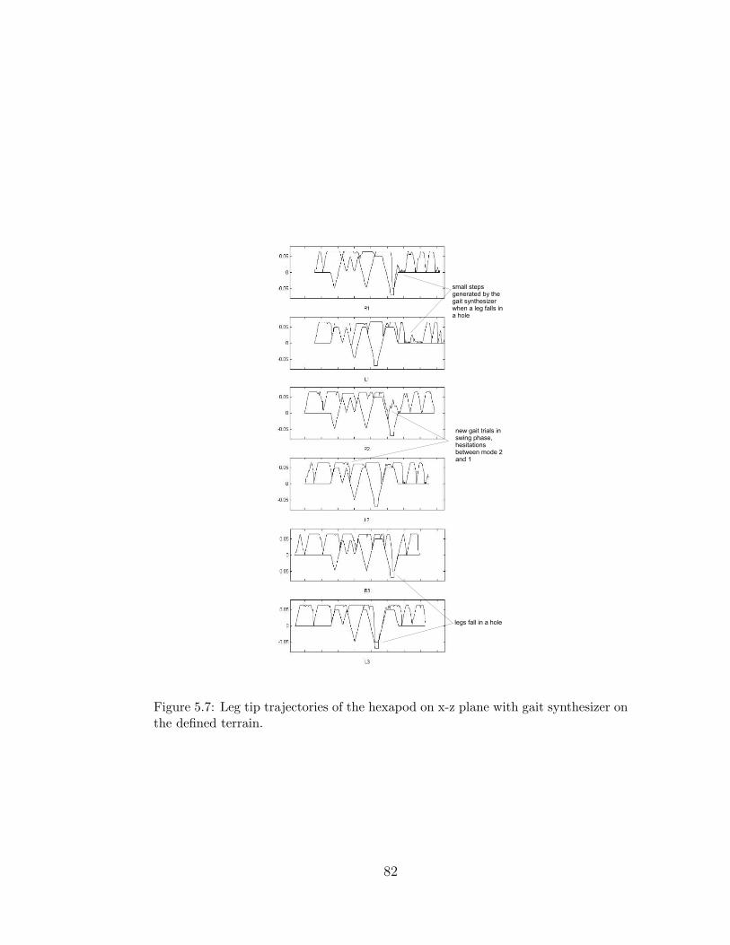
Figure 5.7: Leg tip trajectories of the hexapod on x-z plane with gait synthesizer onthe defined terrain.
82
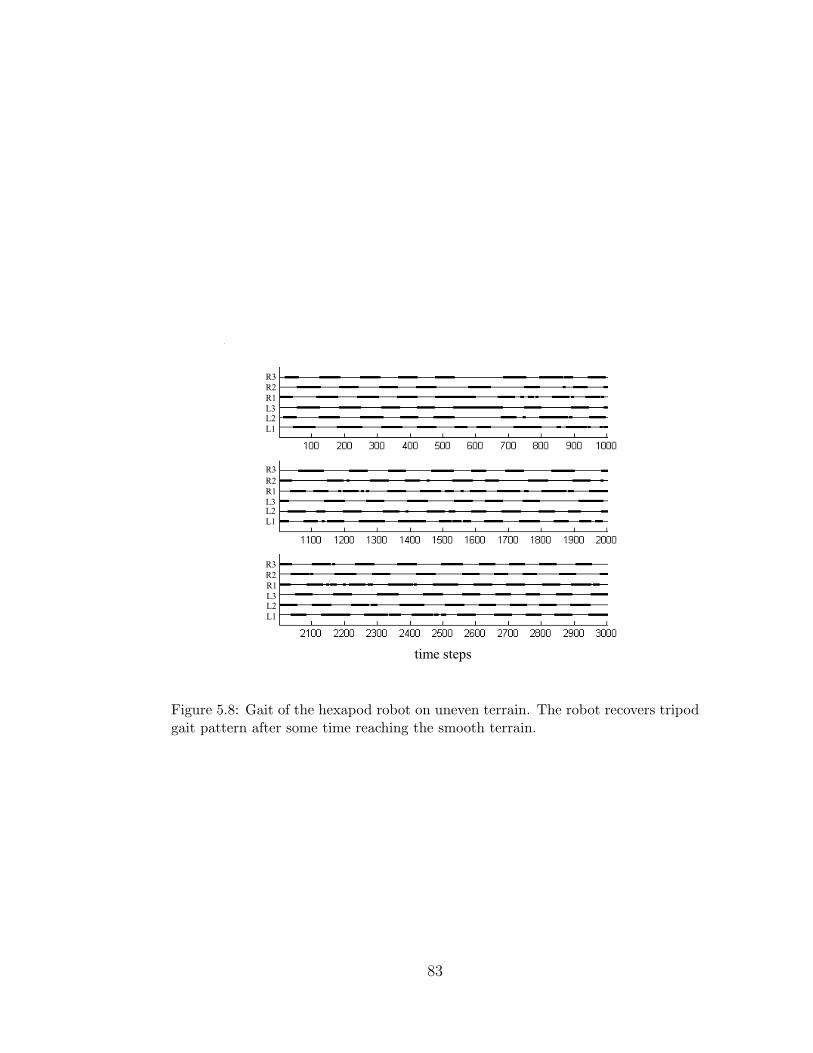
Figure 5.8: Gait of the hexapod robot on uneven terrain. The robot recovers tripodgait pattern after some time reaching the smooth terrain.
83
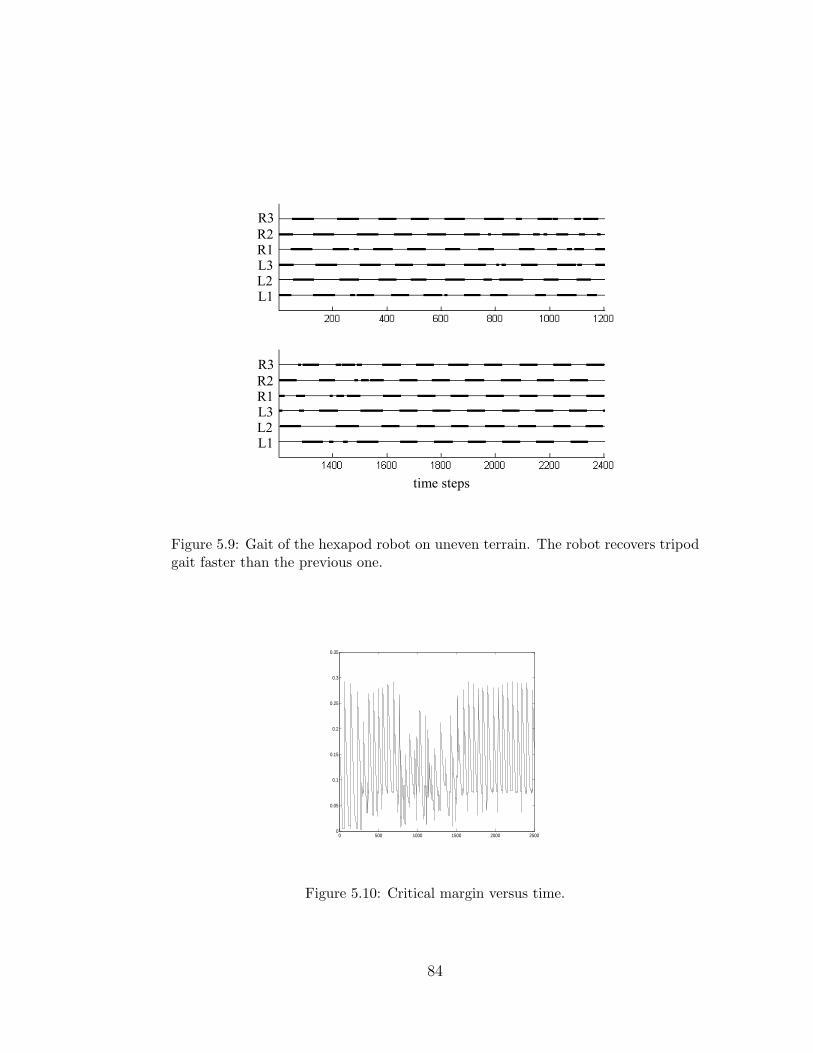
Figure 5.9: Gait of the hexapod robot on uneven terrain. The robot recovers tripodgait faster than the previous one.
0 500 1000 1500 2000 25000
0.05
0.1
0.15
0.2
0.25
0.3
0.35
Figure 5.10: Critical margin versus time.
84
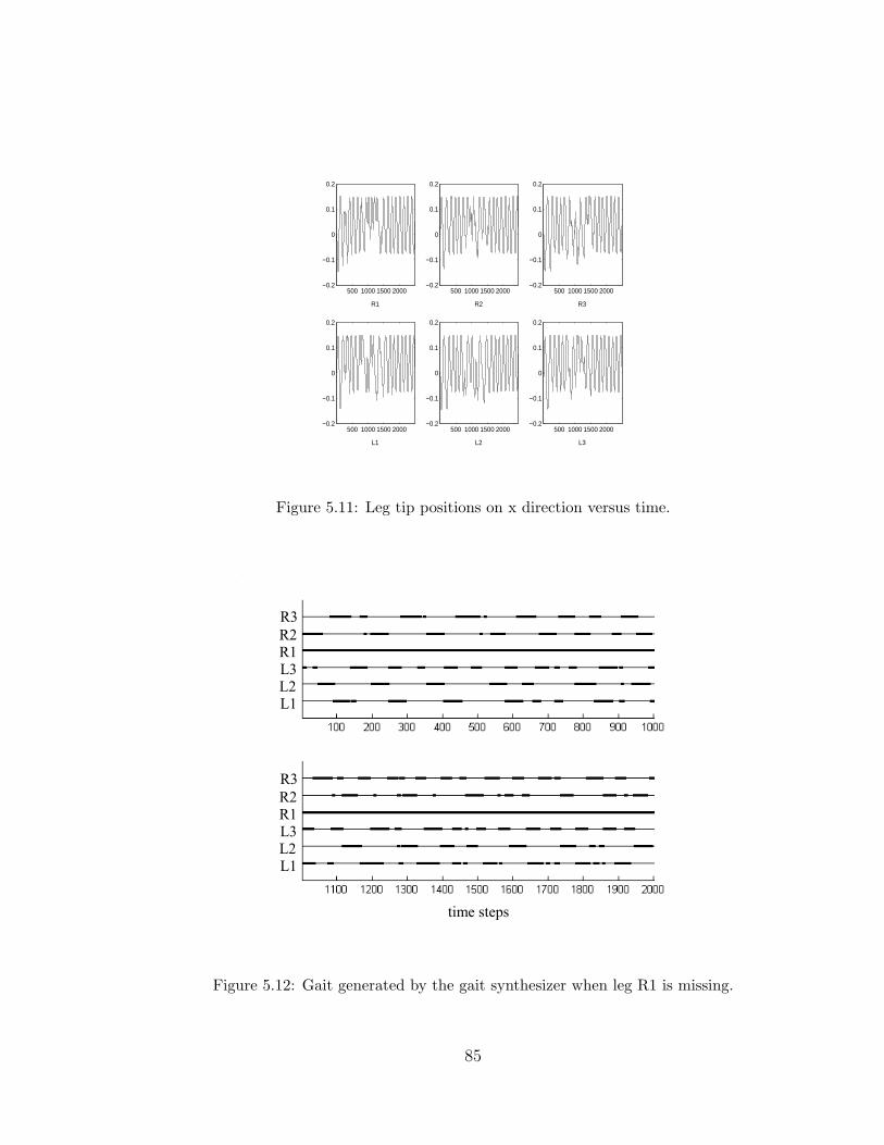
500 1000 1500 2000−0.2
−0.1
0
0.1
0.2
R1
500 1000 1500 2000−0.2
−0.1
0
0.1
0.2
R2
500 1000 1500 2000−0.2
−0.1
0
0.1
0.2
R3
500 1000 1500 2000−0.2
−0.1
0
0.1
0.2
L1
500 1000 1500 2000−0.2
−0.1
0
0.1
0.2
L2
500 1000 1500 2000−0.2
−0.1
0
0.1
0.2
L3
Figure 5.11: Leg tip positions on x direction versus time.
Figure 5.12: Gait generated by the gait synthesizer when leg R1 is missing.
85
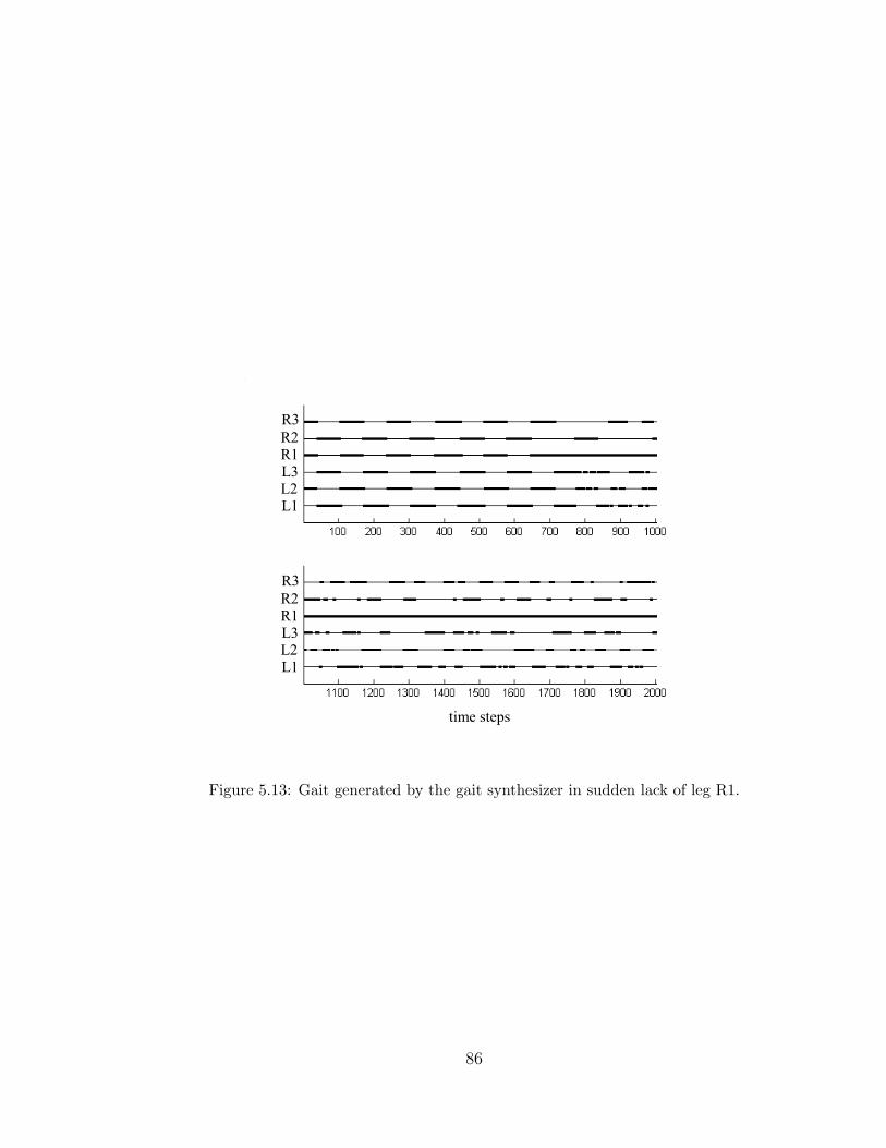
Figure 5.13: Gait generated by the gait synthesizer in sudden lack of leg R1.
86
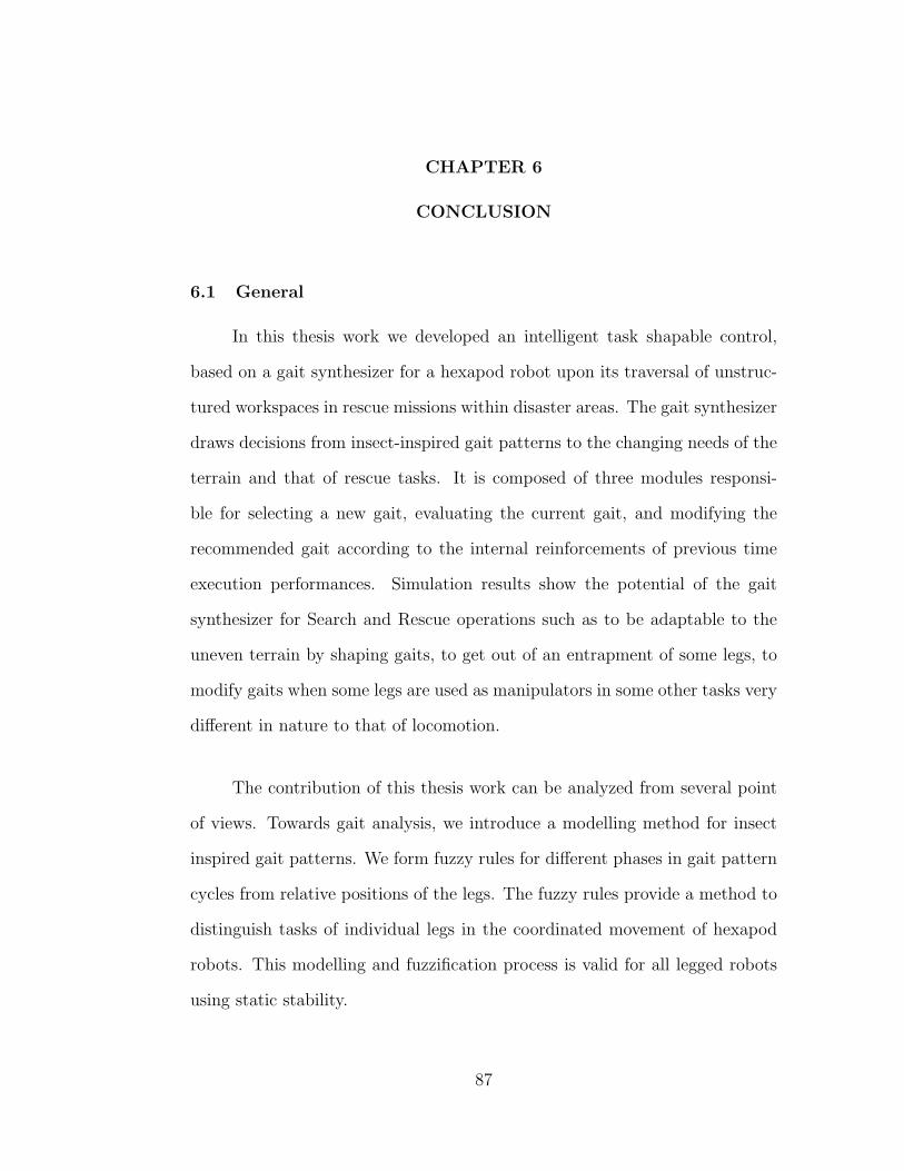
CHAPTER 6
CONCLUSION
6.1 General
In this thesis work we developed an intelligent task shapable control,
based on a gait synthesizer for a hexapod robot upon its traversal of unstruc-
tured workspaces in rescue missions within disaster areas. The gait synthesizer
draws decisions from insect-inspired gait patterns to the changing needs of the
terrain and that of rescue tasks. It is composed of three modules responsi-
ble for selecting a new gait, evaluating the current gait, and modifying the
recommended gait according to the internal reinforcements of previous time
execution performances. Simulation results show the potential of the gait
synthesizer for Search and Rescue operations such as to be adaptable to the
uneven terrain by shaping gaits, to get out of an entrapment of some legs, to
modify gaits when some legs are used as manipulators in some other tasks very
different in nature to that of locomotion.
The contribution of this thesis work can be analyzed from several point
of views. Towards gait analysis, we introduce a modelling method for insect
inspired gait patterns. We form fuzzy rules for different phases in gait pattern
cycles from relative positions of the legs. The fuzzy rules provide a method to
distinguish tasks of individual legs in the coordinated movement of hexapod
robots. This modelling and fuzzification process is valid for all legged robots
using static stability.
87
For legged robots, there are two parts to gait generation; the cyclic action
of the individual legs and the coordination of all the legs to make effective use
of their cycles. Periodic gaits offers this coordination within a pattern with
a fast execution, exhibiting different amount of weakness to irregularities of
the environment. By utilizing a control structure namely the novel gait syn-
thesizer architecture that exhibit intelligent control features such as learning
and adaptability in unstructured environments, we provide exploration among
such periodic gait patterns in order to be mobile and rapid at the same time on
uneven terrain. Besides, the control architecture generates gaits to get out of
entrapment of legs owing to the modifier module as one of the 3 main modules
of the gait synthesizer.
Dynamics of legged robots is complicated because of coupling of individ-
ual legs in the dynamics of the body. We established its similarity to grasping
and manipulation of objects by multi-fingered robot hands. and we consid-
ered locomotion as grasping onto infinitely big, rough, arbitrarily textured
terrain. We make use of multitude of existing works on grasping models with
multi-fingered robot hands to generate the locomotion dynamical equations for
legged robots. Again the derived equations are general enough to be applied
to all legged robots under static stability.
Finally this thesis contributes to the literature on feasibility of au-
tonomous intelligent robots for search and rescue (SAR). We have developed a
coordination control of legs based on gait patterns for fast and secure mobility
of legged robots for the mobility needs in SAR environments. Fast mobility
is ensured by an optimization on speed. Secure mobility is achieved by an
88
optimization of the static stability margin and also by the gait synthesizer
modifying its gait to take out the robot for any motion entrapment. This
deadlockfree locomotion when terrain entrapment or leg failure occur is due to
the ability of our gait synthesizer using successfully the redundancy in multi-
legged robots.
6.2 Future Work
In this thesis we restrict the subject to gait control. In a complete control
structure of a legged robot, the gait synthesizer should undertake more respon-
sibilities than the ones mentioned in this thesis work. The gait synthesizer can
then be further expanded in several ways. By different choice of reinforcement
signals the synthesizer can be trained and adapted to different tasks. We just
give an example of such an adaptation in terms of speed and mobility which
are the main concern of locomotion as our case.
Moreover, for terrain irregularities that are routinely faced in a search
and rescue (SAR) operation (such as specific obstacle types), some control
modules can be added into Gait Modifier Module. Encountering such situa-
tions, the gait synthesizer lets these modules take the control of modifications
held in GMM while still recommending gaits for locomotion.
Also new rule bases can be added to the system for five legged locomotion
so that in a permanent loss of a leg the corresponding rule base can be set in
action. Although we showed that such situations can still be handled by the
gait synthesizer with rules for six legs, addition of such rules will provide more
89
functionality to the gait synthesizer with just a drawback of memory usage.
The analysis in the thesis are made for a two dimensional model of a
hexapod robot locomotion, meaning a straight line walking. The gait synthe-
sizer can be adapted to a real robot by addition of rules for lateral positions
of leg tips and the locomotion can be made over a planar x-y terrain. Also
the working space of the legs must be adapted when orientation of the body
changes. These foreseen changes to the system would not effect the perfor-
mance of the gait synthesizer because the main concept, which is drawing
decisions from gait patterns to the needs of the locomotion, would not change
with these modifications.
An important property of the gait synthesizer is the generated M val-
ues. These values have information about relative functionality of the legs.
Although we just apply to distinguish operation modes of the legs, the other
control modules can also make use of them. For instance, in navigation control
the M vector of the legs can be taken as an input indicating feasibility of a
manoeuvre. For such utilizations the learning algorithm need to be changed.
Because this time not only the comparison with threshold values but also the
value of the M will be meaningful.
90
REFERENCES
[1] Jennifer Casper, Mark Micire, Robin R. Murphy, Issues in Intelligent
Robots for Search and Rescue, .
[2] Ismet Erkmen, Aydan M. Erkmen, Fumitoshi Matsuno, Ranajit Chatter-
jee, Tetsushi Kamegawa, Snake Robots to the Rescue, Serpentine Search
Robots in Rescue Operations, IEEE Robotics and Automation Magazine,
September 2002.
[3] G. Meltem Kulalı, Mustafa Gevher, Aydan M. Erkmen, Ismet Erkmen,
Intelligent Gait Synthesizer for Serpentine Robots, Proceedings of the 2002
IEEE International Conference on Robotics and Automation, Washington,
DC, May 2002.
[4] M. H. Raibert, Legged Robots that Balance, MIT Press, Cambridge, MA,
1986.
[5] S. M. Song, K. J. Waldron, Machines That Walk: The Adaptive Suspension
Vehicle, Cambridge, MA: MIT Press, 1988.
[6] Celaya, E., Porta, J. M., A Control Structure for the Locomotion of a Legged
Robot on Difficult Terrain, IEEE Robotics and Automation Magazine, Vol.
5, No. 2, June 1998, pp. 43-51.
[7] M. J. Randall, A. G. Pipe, A Novel Soft Computing Architecture for the
Control of Autonomous Walking Robots, Soft Computing 4 (2000) 165-185.
91
[8] Shin-Min Song, Kenneth J. Waldron, An Analytical Approach for Gait
Study and Its Applications on Wave Gaits, The International Journal of
Robotics Research, Vol. 6, No. 2, Summer 1987.
[9] J. Dean, A Model of Leg Coordination in the Stick Insect, Carausius Mo-
rosus, I. A geometrical consideration of contralateral and ipsilateral coor-
dination mechanisms between two adjecent legs, Biol. Cybern. 64, 393-402,
1991.
[10] Cynthia Ferrell, A Comparison of Three Insect-inspired Locomotion Con-
trollers, Robotics and Autonomous Systems 16, (1995) 135-159
[11] David Wettergreen, Chunk Thorpe, Gait Generation for Legged Robots,
Proceedings of the IEEE International Conference on Intelligent Robots
and Systems, July 1992.
[12] Hamid R. Berenji, Pratap Khedkar, Learning and Tuning Fuzzy Logic
Controllers Through Reinforcements, IEEE Transactions on Neural Net-
works, Vol. 3, No. 5, September 1992.
[13] Chin-Teng Lin, C.S. George Lee, Neural Fuzzy Systems, Prentice Hall
Inc., 1996.
[14] Jennifer Casper, Mark Micire, Robin R. Murphy, Jeff Hyams, Brian
Menten, Mobility and Sensing Demands in USAR, .
[15] R. Blickhan, R. J. Full, Similarity in Multilegged Locomotion: Bouncing
Like a Monopode, Journal of Comparative Physiology, A(1993) 173:509-
517.
92
[16] Michael H. Dickinson, Claire T. Farley, Robert J. Full, M. A. R. Koehl,
Rodger Kram, Steven Lehman, How Animals Move: An Integrative View,
Science Vol 288 7 April 2000.
[17] Chiel,H., Beer,R., Sterling,L, Heterogenous Neural Networks for Adap-
tive Behaviour in Dynamic Environments, Advances in Neural Information
Processing Systems, 1989,pp. 577-585.
[18] Beer, R. D., Intelligence as Adaptive Behaviour, Academic Press, 1990.
[19] Beer, R. D., Chiel, H. J., Quinn, R. D, Espenschied, K. S., Larsson, P.,
A Distributed Neural Network Architecture for Hexapod Robot Locomotion,
Neural Computation, 4, pp. 356-365, 1992.
[20] Cruse, H., What Mechanisms Coordinate Leg Movement In Walking An-
thropods?, Trends in Neuroscience, 13, pp. 15-21, 1990.
[21] K. Pearson, The control of walking, Scientific American 235:72-86, 1976.
[22] Full, R. J., Blickhan, R., Ting, L. H., Leg design in hexapedal runners, J.
exp. Biol. 158, 369–390.
[23] V.R. Kumar, K.J. Waldron, A Review of Research on Walking Vehicles,
The Robotics Review 1, pp. 243-266, The MIT Press, Cambridge, MA,
1989.
[24] J. Dean, A Model of Leg Coordination in the Stick Insect, Carausius Mo-
rosus, II. Description of the Kinematic Model and Simulation of Normal
Step Patterns, Biol. Cybern. 64, 403-411, 1991.
93
[25] J. Dean, A Model of Leg Coordination in the Stick Insect, Carausius Mo-
rosus, III. Responses to perturbations of normal coordination, Biol. Cy-
bern. 66, 335-343, 1992.
[26] Espenschied, K. S., Chiel, H. J., Quinn, R. D, Beer, R. D., Leg Coordina-
tion Mechanisms in the Stick Insect Applied to Hexapod Robot Locomotion,
Adaptive Behaviour 1 (4), pp. 455-468, 1992.
[27] Espenschied, K. S., Chiel, H. J., Quinn, R. D, Beer, R. D., Biologically-
Inspired Hexapod Robot Control, Proc. 5th Int. Symp. on Robotics and
Manufacturing (ISRAM), 5, pp. 89-94, 1994.
[28] Jung-Min Yang and Jong-Hwan Kim, Optimal Fault Tolerant Gait Se-
quence of the Hexapod Robot with Overlapping Reachable Areas and Crab
Walking, IEEE Transactions on Systems, Man, and Cybernetics- Part A:
Systems and Humans, Vol.29, No. 2, March 1999.
[29] Jung-Min Yang and Jong-Hwan Kim, A fault Tolerant Gait for a Hexapod
Robot over Uneven Terrain, IEEE Transactions on Systems, Man, and
Cybernetics- Part B: Cybernetics, Vol.30, No. 1, February 2000.
[30] Byoung S. Choi, Shin Min Song, Fully Automated Obstacle-Crossing Gaits
for Walking Machines, IEEE Transactions on Systems, Man, and Cyber-
netics, Vol.18, No. 6, November/December 1988.
[31] David Wettergreen, Chuck Thorpe, Gait Generation for Legged Robots,
Proceedings of the IEEE International Conference on Intelligent Robots
and Systems, July 1992 .
94
[32] Robert B. McGhee, Geoffrey I. Iswandhi, Adaptive Locomotion of a Mul-
tilegged Robot over Rough Terrain, IEEE Transactions on Systems, Man,
and Cybernetics, Vol. SMC-9, No. 4, April 1979.
[33] T.D. Barfoot, E.J.P. Earon, G.M.T. D’Eleuterio, A Step in the Right
Direction, Learning Hexapod Gaits Through Reinforcement, International
Symposium on Robotics, Montreal, Canada, 14-17 May 2000.
[34] Alan Calvitti, Randall D. Beer, Analysis of a Distributed Model of Leg
Coordination, I. Individual Coordination Mechanisms, Biol. Cybern. 82,
197-206 (2000).
[35] Porta, J. M., Celaya, E., Gait Analysis for Six-Legged Robots, Techni-
cal Report IRI-DT-9805, Institut de Rob‘otica i inform‘atica Industrial,
Barcelona, March 1998.
[36] E. Celaya, J.M. Porta, V. Ruz de Angulo, Reactive Gait Generation for
Varying Speed and Direction, First International Symposium on Climbing
and Walking Robots, 1998.
[37] U. Saranlı, M. Buehler, D. E. Koditschek, Design, Modeling and Prelimi-
nary Control of a Compliant Hexapod Robot, IEEE Int. Conf. on Robotics
and Automation, San Fransisco, CA (April 2000).
[38] Long-Ji Lin, Self-Improving Reactive Agents Based On Reinforcement
Learning, Planning and Teaching, Machine Learning, 8, 293-321, 1992.
[39] Andrew G. Barto, Richard S. Sutton, and Christopher J.C.H Watkins,
Learning and Sequential Decision Making, Learning and computational
neuroscience, MIT Press, 1990.
95
[40] George J. Klir, Tina A. Folger, Fuzzy Sets, Uncertainty, and Information,
Prectice Hall.
[41] Sutton, R.S., Learning to predict by the methods of temporal differences,
Machine Learning, 3:9-44 1988.
[42] K.S. Fu, R.C. Gonzalez, C.S.G. Lee, Robotics: Control, Sensing, Vision,
and Intelligence, McGraw-Hill.
[43] John J. Craig, Introduction to Robotics, Mechanics and Control, Addison-
Wesley Publishing Company.
[44] Kathryn W. Lilly, Efficient Dynamic simulation of robotic mechanisms,
Kluwer Academic Publishers, 1993.
[45] Robert J. Schilling, Fundamentals of Robotics, Analysis and Control,
Prentice Hall, 1990.
[46] Michael McKenna, David Zeltzer, Dynamic simulation of autonomous
legged locomotion, In Computer Graphics (SIGGRAPH proceedings), vol-
ume 24. ACM, August 1990.
[47] Jelena Godjevac, Comparative Study of Fuzzy Control, Neural Network
Control and Neuro-Fuzzy Control, Technical Report, No: 103/95, February
1995.
[48] Zexiang Li, Ping Hsu, Shankar Sastry, Grasping and Coordinated Manip-
ulation by a Multifingered Robot Hand, International Journal of Robotics
Research, Vol. 8, No. 4, August 1989.
96
[49] J. Kerr, An analysis of multifingered hands, Ph.D. Dissertation. Mechan-
ical Engineering, Stanford University, 1984.
[50] David Baraff, Physically based modelling: Principles and Practice, Sig-
graph 97 course notes.
[51] Arlene B. A. Cole, John E. Hauser, S. Shankar Sastry, Kinematics and
Control of Multifingered Hands with Rolling Contact, IEEE Transactions
on Automatic Control, Vol. 34, No. 4, April 1989.
[52] Lin C. T., Lee C. S. G., Neural Network Based Fuzzy Logic Control and
Decision System, IEEE Transactions on Comput., 40(12), pp. 1320-1336,
1991.
[53] Jang R., Neuro-Fuzzy Modeling: Architectures, Analyses and Aplications,
PhD Thesis, University of California, Berkeley, July 1992.
[54] Nauck D., Kruse R., Neuro-Fuzzy Systems for Function Approximation,
4th International Workshop Fuzzy-Neuro Systems, 1997.
97