intelligent controller based on raspberry pistudentnet.cs.manchester.ac.uk/resources/library/... ·...
TRANSCRIPT
INTELLIGENT CONTROLLER BASED ON
RASPBERRY PI
A dissertation submitted to the University of Manchester for the
degree of Master of Science in the Faculty of Engineering and Physical
Sciences
2014
FEIDIAS IOANNIDIS
SCHOOL OF COMPUTER SCIENCE
1 | Page
Table of Contents
List of Figures ........................................................................................................ 3
List of Tables ......................................................................................................... 7
Abstract ................................................................................................................ 8
Declaration ........................................................................................................... 9
Intellectual Property Statement ........................................................................... 10
Acknowledgements .............................................................................................. 11
1. Introduction ..................................................................................................... 12
1.1 Aim and Objectives .................................................................................................. 12
1.2 Project Context ........................................................................................................ 13
1.3 Deliverables ............................................................................................................. 13
1.4 Dissertation structure .............................................................................................. 14
2. Background ................................................................................................... 15
2.1 Control Theory ......................................................................................................... 15
2.1.1 Transfer function .............................................................................................................. 16
2.1.2 Continuous time and discrete time in control theory ...................................................... 18
2.1.3 s and z domains for the transfer function ........................................................................ 18
2.1.4 Deviation variables in control theory ............................................................................... 19
2.2 PID control ............................................................................................................... 20
2.2.1 PID Tuning techniques ...................................................................................................... 22
2.3 Hardware components and software tools ............................................................. 25
2.3.1 Raspberry Pi ...................................................................................................................... 25
2.3.2 Python programming language ........................................................................................ 26
2.3.3 Input and output resolution ............................................................................................. 27
3. Design and Methodology for PID Controllers ................................................. 28
3.1 Methodology ........................................................................................................... 28
3.2 System block diagram .............................................................................................. 29
3.3 System identification methods ................................................................................ 31
3.3.1 Step response ................................................................................................................... 31
3.3.1.1 63.2% and Tangent Method .................................................................................... 32
3.3.1.2 Method of Moments ................................................................................................ 34
3.3.1.3 2-point method ........................................................................................................ 35
3.3.2 Parameter Estimation ....................................................................................................... 37
3.3.2.1 Pseudorandom Binary Signal (PRBS) ........................................................................ 38
3.3.2.2 Least squares method .............................................................................................. 39
3.4 Tuning techniques ................................................................................................... 43
4. Implementation for PID Controllers ............................................................... 44
2 | Page
4.1 Building the system ................................................................................................. 44
4.1.1 Hardware components ..................................................................................................... 47
4.2 Interfacing with hardware components .................................................................. 48
4.2.1 Input devices ..................................................................................................................... 48
4.2.2 Output devices .................................................................................................................. 52
4.3 PID controller implementation ................................................................................ 57
4.3.1 Initial experiment ............................................................................................................. 57
4.3.1.1. Step input ................................................................................................................. 58
4.3.1.2. PRBS ......................................................................................................................... 59
4.3.2 System identification ........................................................................................................ 60
4.3.2.1. Step response .......................................................................................................... 60
4.3.2.2. Parameter estimation .............................................................................................. 61
4.3.3 PID controller tuning......................................................................................................... 62
4.3.4 PID controller loop implementation ................................................................................. 64
4.3.5 Other practical considerations for PID controller ............................................................. 65
4.4 Complete system demonstration ............................................................................ 68
5. Evaluation, Testing and Results ..................................................................... 72
5.1 Measurement tools ................................................................................................. 72
5.2 Hardware components evaluation and testing ....................................................... 73
5.3 System model evaluation ........................................................................................ 75
5.3.1 Step response ................................................................................................................... 76
5.3.2 Parameter estimation ....................................................................................................... 79
5.3.3 Comparison of system identification between step response and parameter estimation
82
5.4 PID controller evaluation ......................................................................................... 84
5.4.1 On-off controller and MATLAB generated control ........................................................... 85
5.4.2 Step response ................................................................................................................... 89
5.4.3 Parameter estimation ....................................................................................................... 92
5.4.4 Comparison of PID control between step response and parameter estimation .............. 96
5.5 Project results .......................................................................................................... 98
6. Conclusion and Future Work ........................................................................ 101
6.1 Conclusions ............................................................................................................ 101
6.2 Future Work .......................................................................................................... 103
References ......................................................................................................... 105
Word count: 27 412
3 | Page
List of Figures
Figure 2.1, closed loop control structure .................................................................... 16
Figure 2.2, PID control scheme, r(t) is the reference value at time t, e(t) is the error
value at time t, u(t) is the output of the controller (input of the process) at time t and
y(t) is the output of the system at time t ..................................................................... 20
Figure 2.3, three different types of controllers. Blue line represents P only controller,
red line represents PI controller and green line represents PID controller (values
used, Kp = 2, Ki = 0.35, Kd = 1.3) .................................................................................. 22
Figure 2.4, simulation of PID controlled system close to critically damped with Kp = 2,
Ki = 0.35 and Kd = 1.3 ................................................................................................... 24
Figure 2.5, Raspberry Pi, highlighted with the red rectangle are the 26 pins ............. 26
Figure 3.1. The three parts of the project (Input, Controller, Output), their
connection and the connection between them and various devices and sensors. .... 28
Figure 3.2. The block diagram of the system. Shows the four components of the
system and their inputs and outputs. .......................................................................... 30
Figure 3.3. The block diagram of the temperature control system. Shows the
hardware components of the system. ......................................................................... 31
Figure 3.4, step response of a system and derivation of the three parameters K, L
and T from the plot (L = A, T = B - A, K =K / process input change) ............................. 33
Figure 3.5, example of step response of a system. a) Shows the output of the system.
Dashed line is the smoothened step response output, solid line is the output
measurement with noise. b) Shows the process input/controller output setting
during the same time (change between 10 and 10.5 represents the step) ................ 34
Figure 3.6. The calculation of gain K, time constant T and time delay L using the
method of moments .................................................................................................... 35
Figure 3.7, step response of a system and derivation of the three parameters K, L
and T from the plot using the 2-point method ............................................................ 36
Figure 3.8. General representation of the parameter estimation method. Input and
output are used to produce the parameter vector and therefore the transfer
function ........................................................................................................................ 37
Figure 3.9. Example of PRBS Signal, with 1 and -1 as the two possible values ........... 39
Figure 3.10. Graphical representation of the least square error procedure used to
calculate θ .................................................................................................................... 40
Figure 3.11. Graph of V(θ) and how differentiation can be used to find the minimum
value ............................................................................................................................. 41
Figure 3.12. First table contains input and output data in deviation form at discrete
time k, second table is the Φ matrix and third table is the Y matrix ........................... 42

4 | Page
Figure 4.1. Design of the aluminium block. View of the whole block, front view
showing the holes, top view showing the cuts and top view showing the holes. All
dimensions are in mm. ................................................................................................. 46
Figure 4.2. Circuit diagram of the connection between the sensor and Raspberry Pi 49
Figure 4.3. Physical wiring of the temperature sensor. Red wire is voltage supply
(3.3V), black wire is the ground, brown wire is the clock and yellow wires are used to
provide data to the Raspberry Pi ................................................................................. 50
Figure 4.4. Physical wiring of ADC. Red wire is voltage supply (3.3V), black wire is
ground, yellow wires are SDA and SCL and grey wire is used to give I2C address (0x49)
...................................................................................................................................... 51
Figure 4.5. ADC circuit diagram. A0 – A4 of the ADC are connected to the analogue
source. .......................................................................................................................... 51
Figure 4.6. Circuit diagram of Raspberry Pi and AD5662 DAC .................................... 53
Figure 4.7. A valid write sequence of the 24 bits digital value .................................... 53
Figure 4.8. The transmitted bit sequence to the DAC from the microcontroller........ 53
Figure 4.9. The __inint__() method of the DAC class .................................................. 54
Figure 4.10. The write() method of the DAC class ....................................................... 54
Figure 4.11. The clock() method of the DAC class ....................................................... 54
Figure 4.12. Circuit diagram of the LCD screen. A potentiometer is also used........... 55
Figure 4.13. Physical wiring of the LCD screen with the Raspberry Pi. ....................... 56
Figure 4.14. Circuit diagram of the heaters and the external power supply. DAC
output is amplified by the power supply to power the heaters. ................................. 56
Figure 4.15. Instantiation of the DAC and SHT1x classes ............................................ 57
Figure 4.16. Code used to bring the system to a steady state. Input is 20%. ............. 58
Figure 4.17. The steady_state() method used to identify whether the system has
reached a steady state ................................................................................................. 58
Figure 4.18. Code used for the PRBS experiment. Probability p used is 0.1 (10%
chance). ........................................................................................................................ 59
Figure 4.19. The system_response() method code and how it is used to estimate
time delay L. ................................................................................................................. 60
Figure 4.20. Code of the value_closer() method used to estimate the time constant
T. ................................................................................................................................... 61
Figure 4.21. Code used to form the φ matrix .............................................................. 62
Figure 4.22. Code used to calculate the θ vector. ....................................................... 62
Figure 4.23. Calculation of the three gains using open-loop Ziegler-Nichols rules. .... 63
Figure 4.24. Code from the pidsim library for the calculation of the three gains using
open-loop Ziegler-Nichols rules. .................................................................................. 63
Figure 4.25. Implementation of the PID controller loop. ............................................ 64
Figure 4.26. Integrator windup effect. Top graph shows the process output and
bottom graph shows controller output ....................................................................... 66
5 | Page
Figure 4.27. Implementation of the anti-windup method. Controller output clamping
is used and the error stops accumulating. ................................................................... 67
Figure 4.28. The complete system with all components (Raspberry Pi, breadboard,
aluminium block, external power supply) connected. ................................................ 68
Figure 4.29. The initial screen message and the three buttons (two navigation
buttons and one submit button). ................................................................................ 69
Figure 4.30. The message on the screen asks the user to select one of the three
modes of operation (step response, least squares or using existing gains). ............... 69
Figure 4.31. The message displayed on the screen asking the user to select the
desired temperature. ................................................................................................... 70
Figure 4.32. Message on the screen informing the user of the current temperature
and current power percentage used. .......................................................................... 71
Figure 5.1, readings produced by the ADC for the 3 different voltage supply settings
tested (each setting was measured for 1 second). Values above the lines denote the
voltage input setting from the accurate voltage supply. For the 1st second the voltage
input setting was 1000 mV, for the 2nd second it was 1000.1 mV and for the 3rd
second it was 1000.2 mV. ............................................................................................ 74
Figure 5.2, DAC voltage output in mV measured by the voltmeter for 2 different
digital values (3000 and 3001). .................................................................................... 75
Figure 5.3. The evaluation procedure used to validate the accuracy of the model
compared to the physical system. Same input is used and outputs are compared ... 76
Figure 5.4. The step response of the process. The blue line shows the output of the
process, the red horizontal line shows the process gain K, the horizontal black line
shows the value equal to 63.2% of K, the vertical black line shows the time that
63.2% was reached which represents time constant T, the green line shows time
delay L. ......................................................................................................................... 77
Figure 5.5. The process input for the step input experiment. The input steps from
20% to 30% (percentage of DAC amplified output). ................................................... 78
Figure 5.6. Comparison of the system actual output and the simulation output using
the same input. Output is expressed as the amplitude of deviation from the initial
temperature. ................................................................................................................ 79
Figure 5.7. The PRBS signal used as the input for the parameter estimation
experiment. The possible values are 0% and 100%. .................................................... 80
Figure 5.8. The output to the PRBS signal for the parameter estimation experiment.
The output is expressed as temperature versus time. ................................................ 81
Figure 5.9. Comparison of the system measured output (dotted curve) and the
simulation output using the same input. Output is expressed as the amplitude of
deviation from the initial temperature. ....................................................................... 82
Figure 5.10. The output of the on-off controller. The red dotted line represents the
set point and the blue solid line represents the output. ............................................. 86

6 | Page
Figure 5.11. The input of the on-off controller. Input is represented as a percentage
voltage. ......................................................................................................................... 86
Figure 5.12. Accuracy evaluation of MATLAB generated transfer function model .... 87
Figure 5.13. Output of the control experiment using MATLAB generated PID gains (Kp
= 92.64, Ki = 2.27, Kd = 940.29). Green dashed line indicates the rise time. ............... 88
Figure 5.14. The input of the control experiment using MATLAB generated gains.
Input is represented as a percentage voltage. ............................................................ 88
Figure 5.15. PID control experiment using the gains produced by the step response
method. The blue solid curve represents the output, the green dashed line indicates
the response/rise time and the red dotted line represents the set point. ................. 89
Figure 5.16. The input for the first PID control experiment using step response
produced gains. Input is expressed as a percentage. .................................................. 90
Figure 5.17. Second PID control experiment using the gains produced by the step
response method. The blue solid curve represents the output, the green dashed line
indicates the response time and the red dotted line represents the set point. ......... 91
Figure 5.18. The input for the second PID control experiment using step response
produced gains. Input is expressed as a percentage. .................................................. 92
Figure 5.19. First PID control experiment using the gains produced by the parameter
estimation method. The blue solid curve represents the output, the green dashed
line indicates the response/rise time and the red dotted line represents the set
point. ............................................................................................................................ 93
Figure 5.20. The input for the first PID control experiment using parameter
estimation produced gains. Input is expressed as a percentage................................. 94
Figure 5.21. Second PID control experiment using the gains produced by the
parameter estimation method. The blue solid curve represents the output, the green
dashed line indicates the response/rise time and the red dotted line represents the
set point. ...................................................................................................................... 95
Figure 5.22. The input for the second PID control experiment using parameter
estimation produced gains. Input is expressed as a percentage................................. 96
Figure 5.23. Output of the controller for a set point of 35oC. Controller uses
parameter estimation gains. Green dashed line indicates the rise time. ................... 99
Figure 5.24. Output of the controller for a set point of 40oC. Controller uses
parameter estimation gains. Green dashed line indicates the rise time. ................... 99
7 | Page
List of Tables
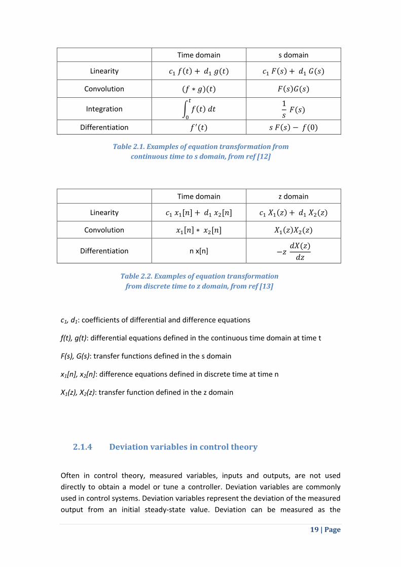
Table 2.1. Examples of equation transformation from continuous time to s domain 19
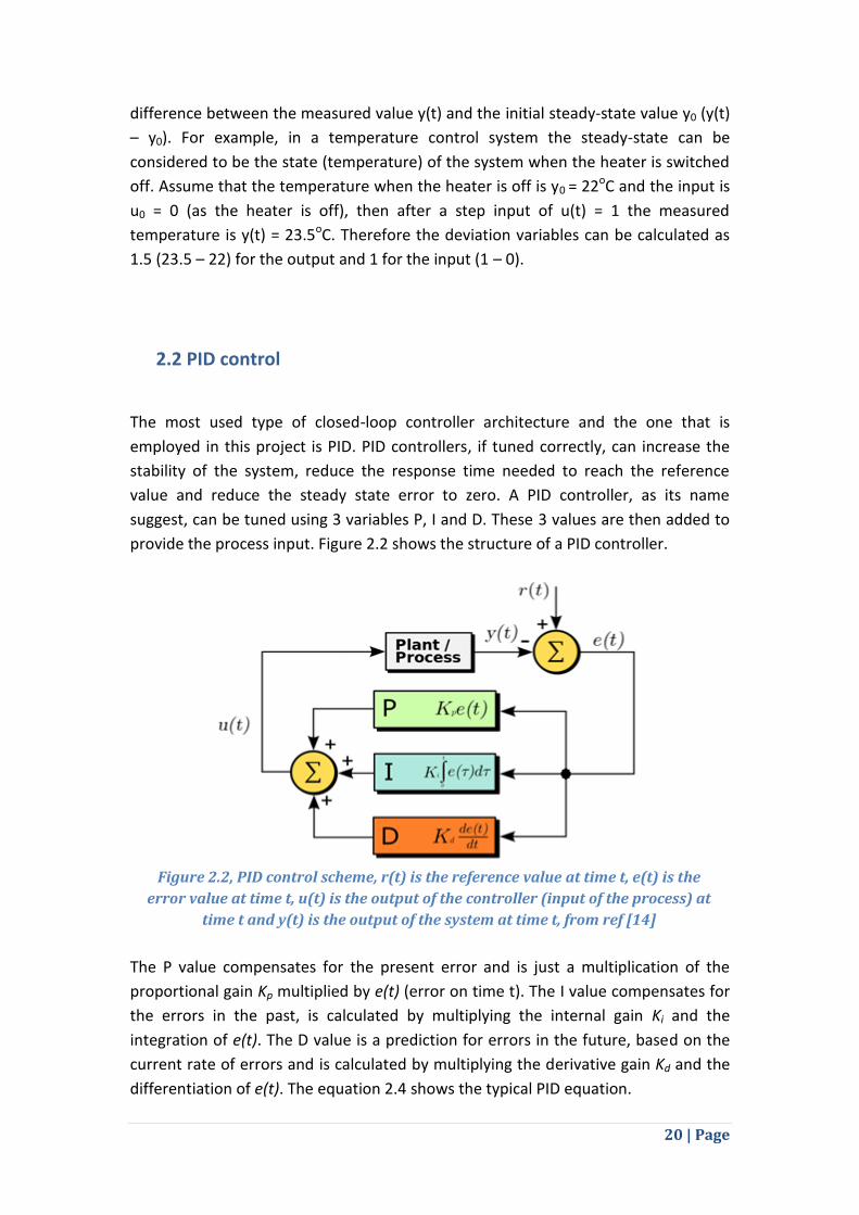
Table 2.2. Examples of equation transformation from discrete time to z domain ..... 19
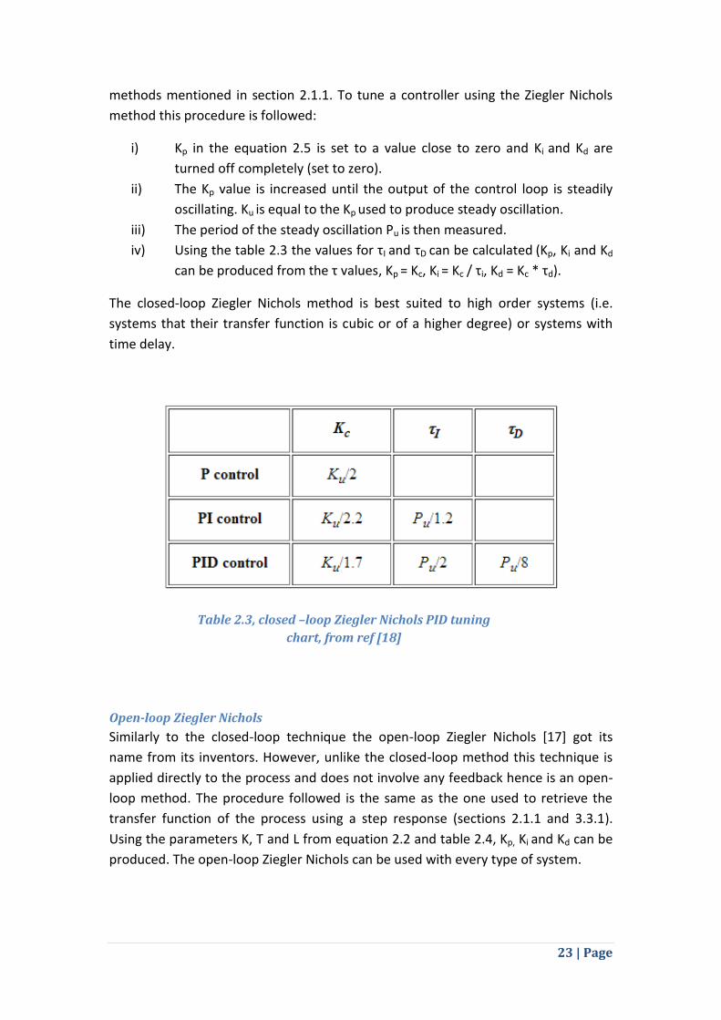
Table 2.3, closed –loop Ziegler Nichols PID tuning chart ............................................ 23
Table 2.4, open-loop Ziegler Nichols PID tuning chart ................................................ 24
Table 5.1. Comparison of the PID gains obtained by the step response model and
parameter estimation model (Ziegler Nichols open-loop tuning technique used for
both). ............................................................................................................................ 84
Table 5.2. Comparison of the four techniques in terms of oscillations, response/rise
time, input range, overshoot and steady state error .................................................. 98
8 | Page
Abstract
Intelligent controllers are used everywhere, from a cruise control on a car to an air conditioning system. They are primarily used to provide corrective actions to maintain the stability of the system and produce an output close to the reference point selected by the user.
There are many challenges related to the development of a controller. The type of the controller needed, the hardware components that will be used, the system identification technique that will be used to identify the mathematical model of the process and the tuning method are some of the considerations that should be made. All these considerations are part of this MSc project. The aim of this project is to design and implement an intelligent, efficient and accurate PID (Proportional, Integral, Derivative) controller based on the Raspberry Pi platform.
The purpose of this report is to describe the PID controller created, as well as to cover all of the challenges related to the development of a PID controller. It provides an insight into the background information related to the project. Important topics such as hardware interfacing, Ziegler-Nichols PID tuning, step response and parameter estimation identification techniques are extensively discussed. Implementation details and practices are also included. Additionally, experimental data is presented to demonstrate the accuracy and performance of the PID controller and its components.
After the system was evaluated, it was demonstrated that the controller met the
expectations in terms of performance and efficiency. The PID controller successfully
controlled the temperature of the system. Furthermore, the transfer function
models produced proved accurate. The control was successful especially when using
the controller parameters (gains) produced by the parameter estimation system
identification technique, which proved to be more effective than step response.

9 | Page
Declaration
No portion of the work referred to in the dissertation has been submitted in support
of an application for another degree or qualification of this or any other university or
other institute of learning.
10 | Page
Intellectual Property Statement
I. The author of this dissertation (including any appendices and/or
schedules to this dissertation) owns certain copyright or related rights in
it (the “Copyright”) and s/he has given The University of Manchester
certain rights to use such Copyright, including for administrative
purposes.
II. Copies of this dissertation, either in full or in extracts and whether in hard
or electronic copy, may be made only in accordance with the Copyright,
Designs and Patents Act 1988 (as amended) and regulations issued under
it or, where appropriate, in accordance with licensing agreements which
the University has entered into. This page must form part of any such
copies made.
III. The ownership of certain Copyright, patents, designs, trade marks and
other intellectual property (the “Intellectual Property”) and any
reproductions of copyright works in the dissertation, for example graphs
and tables (“Reproductions”), which may be described in this dissertation,
may not be owned by the author and may be owned by third parties.
Such Intellectual Property and Reproductions cannot and must not be
made available for use without the prior written permission of the
owner(s) of the relevant Intellectual Property and/or Reproductions.
IV. Further information on the conditions under which disclosure, publication
and commercialisation of this dissertation, the Copyright and any
Intellectual Property and/or Reproductions described in it may take place
is available in the University IP Policy (see
http://documents.manchester.ac.uk/display.aspx?DocID=487), in any
relevant Dissertation restriction declarations deposited in the University
Library, The University Library’s regulations (see
http://www.manchester.ac.uk/library/aboutus/regulations) and in The
University’s Guidance for the Presentation of Dissertations.

11 | Page
Acknowledgements
I would like to thank my supervisor Prof. Thomas Thomson for his support, guidance
and availability during all stages of this project. I am also grateful to Jack Warren for
his help especially with the design of the aluminium block. I would also like to thank
Stephen Rhodes for his help with hardware components. Finally, I would like to
thank my family and friends for their love and encouragement.
12 | Page
1. Introduction
Control systems date back to ancient times. The first feedback control systems are
believed to be “water clocks” used to keep time over 1000 years ago by regulating
the liquid flow into or out of a vessel [1]. Control systems are used to manipulate the
state of the controlled process without the need for constant input or corrections by
the user. Major progress in the development of feedback control systems appeared
in the first decades of the last century, following the discovery of the Laplace and
Fourier transforms.
Characteristics of a good control system are [2]:
Stability, the system should not oscillate.
Fast response/rise time, the system should reach the reference point as fast
as possible.
Zero steady-state error, when the system is stable the difference between
the output of the system and the reference output should be close to zero.
Tracking of the reference point, the output should be as close to the
reference point as possible.
This chapter presents basic information about the project such as: i) the aims and
the objectives of the project, ii) the project context, iii) the deliverables of the
project and iv) an overview of the remainder of the report.
1.1 Aim and Objectives
The main aim of this project is to design and develop an intelligent controller based
on the Raspberry Pi [3] platform that can be used to control the temperature of a
high power laboratory power supply. A custom controller based on the Raspberry Pi
platform can be an effective and inexpensive alternative to commercial, off the shelf,
expensive PID controllers. Ideally the controller should be readily adaptable to
control other systems as well, e.g. control of current to produce a magnetic field.
The controller produced should be efficient and accurate. It should be able to receive
an input from a sensor in volts, convert it to the desired format and, based on that,
provide a control output to a device, e.g. control the rotation speed of a fan.

13 | Page
Objectives of the project include:
Assemble the required hardware components including the Raspberry Pi, a
temperature sensor, a fan/heater etc.
Develop a mathematical model for the process that will be controlled.
Implement the program that incorporates the PID controller logic and use a
tuning technique to tune the controller.
Evaluation of the effectiveness of the assembled system.
1.2 Project Context
To meet the objectives stated above, knowledge and use of control theory [4]
principles is required. Control theory is a branch of mathematics and engineering
where the purpose is to modify the behaviour of a dynamic system with inputs (e.g.
input from a temperature sensor) that changes over time. Control theory principles
are used to develop the mathematical model and to implement the logic of the
controller. A controller can be implemented in many different ways, the type of
controller that was implemented in this project is PID (Proportional, Integral,
Derivative) [5-6]. Therefore, methods related to the implementation and tuning of a
PID controller are studied and used.
The implementation of the controller is based on the Raspberry Pi platform. The
hardware components used are standard, off-the-shelf hardware components, e.g.
temperature sensor, LCD screen etc.
1.3 Deliverables
The main deliverable of the project is to create a working intelligent controller,
based on the Raspberry Pi platform, for energy efficient thermal management of
instruments or devices. The controller should be able to receive an input from a
temperature sensor and convert it to the desired format (degrees Celsius). The input
should then influence the control procedure, which will produce an output. That
output will be used by a fan/heater, e.g. rotation speed of a fan or current supplied
to a heater. An additional deliverable can be the design of the system with sufficient
flexibility so that it can be used for other applications. A specific example is the

14 | Page
control of current to produce a magnetic field. A further goal is the integration of the
controller in a stand-alone device.
1.4 Dissertation structure
The remainder of this report is structured as follows:
Chapter 2 - Background: in this chapter fundamental information regarding
the background knowledge needed for understanding the project is
presented. Areas covered are: i) control theory, ii) PID controller and iii)
Hardware components and software tools.
Chapter 3 – Design and methodology for PID controllers: this chapter
contains the design decisions and the methodology followed to develop the
controller. It includes block diagrams of the system, details about the system
identification techniques and PID tuning techniques.
Chapter 4 – Implementation for PID controllers: implementation details are
included in this chapter. Such details include how the interfacing between
the hardware components and the Raspberry Pi is done and how the system
identification techniques and the PID tuning method are implemented.
Chapter 5 – Evaluation and results: this chapter contains details about the
evaluation procedure for all parts of the system and the results produced.
Parts that are evaluated include the hardware components, the system
identification techniques and the PID control.
Chapter 6 – Conclusion and future work: the final chapter contains a
summary of the report, as well as suggestions regarding possible future
additions and improvements.
15 | Page
2. Background
This chapter presents the principles used to design and develop the PID controller.
The first section contains information about control theory, the fundamentals
behind the design of every controller. Subjects such as open and closed loop control
systems, components of the controlled system and transfer functions are covered in
this chapter.
The second section contains information about PID controllers, the type of controller
that is used in this project. P, I and D gains are described in this section, as well as
PID tuning.
The third and last section describes the Raspberry Pi platform and the other
hardware components that are used in the project. The programming language used
in this project is also described.
2.1 Control Theory
Control theory is a branch of mathematics and engineering with the purpose of
modifying the behaviour of a dynamic system with inputs (e.g. input from a
temperature sensor) that changes over time. The main objective of control theory is
stability. Usually (in closed loop systems) stability is achieved by continually taking
measurements and making adjustments to the system, this procedure forms a loop.
Usually a loop in control theory consists of: i) the referenced value or set point (the
desired output, provided by the user or some other part of a larger system), ii) the
controller, iii) the process (e.g. the heater) and iv) sensors.
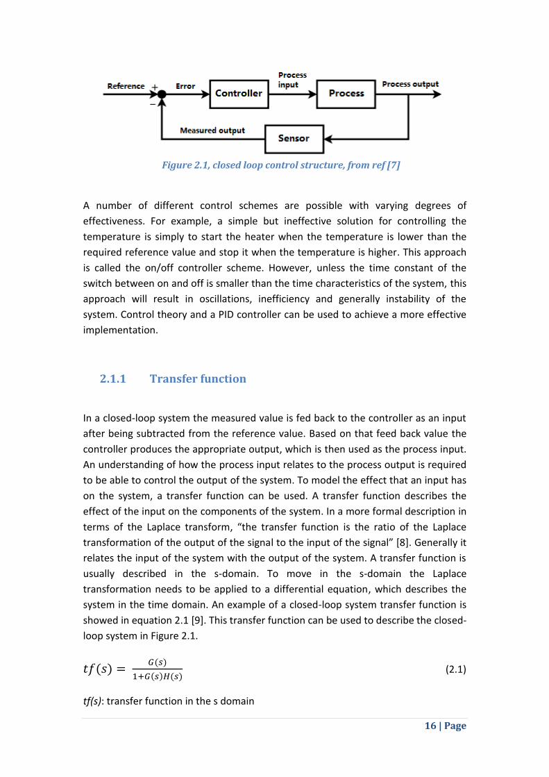
Systems are divided in two basic categories in terms of control structure, open-loop systems and closed-loop systems. In a closed-loop system, the output of the process is measured and subtracted from the reference value, producing the error value. The error value is then passed to the controller, which will then make various calculations and modify the process input accordingly, producing a new process output. The procedure is repeated in a continuous manner. In an open-loop system the output is not fed back to the controller, thus it cannot influence the input. Closed-loop is generally preferred as they react to disturbances better, can stabilize inherently unstable systems and track the reference value better. Figure 2.1 shows the structure of a closed-loop system.
16 | Page
A number of different control schemes are possible with varying degrees of
effectiveness. For example, a simple but ineffective solution for controlling the
temperature is simply to start the heater when the temperature is lower than the
required reference value and stop it when the temperature is higher. This approach
is called the on/off controller scheme. However, unless the time constant of the
switch between on and off is smaller than the time characteristics of the system, this
approach will result in oscillations, inefficiency and generally instability of the
system. Control theory and a PID controller can be used to achieve a more effective
implementation.
2.1.1 Transfer function
In a closed-loop system the measured value is fed back to the controller as an input
after being subtracted from the reference value. Based on that feed back value the
controller produces the appropriate output, which is then used as the process input.
An understanding of how the process input relates to the process output is required
to be able to control the output of the system. To model the effect that an input has
on the system, a transfer function can be used. A transfer function describes the
effect of the input on the components of the system. In a more formal description in
terms of the Laplace transform, “the transfer function is the ratio of the Laplace
transformation of the output of the signal to the input of the signal” [8]. Generally it
relates the input of the system with the output of the system. A transfer function is
usually described in the s-domain. To move in the s-domain the Laplace
transformation needs to be applied to a differential equation, which describes the
system in the time domain. An example of a closed-loop system transfer function is
showed in equation 2.1 [9]. This transfer function can be used to describe the closed-
loop system in Figure 2.1.
(2.1)
tf(s): transfer function in the s domain
Figure 2.1, closed loop control structure, from ref [7]
17 | Page
G(s): transfer function of the controller and the process
H(s): transfer function of the feedback elements (e.g. sensors)
Identifying the transfer function of a process can be a challenging task. The transfer
function of a process can be obtained by two methods. The first method is to model
the process as a set of differential mathematical equations using physical laws, e.g.
Newton’s laws, or an engineering model and then apply the Laplace transformation
to that model. The second method is to provide a specific input to the process and,
based on the output, define the transfer function. Techniques that use inputs and
outputs to define the transfer function are called black box system identification
techniques, as no deep knowledge of the system is needed. Common inputs for this
second category of methods include a step or an impulse. The first method is usually
more accurate but requires a full understanding of the process and ability to
translate the process to a mathematical model using laws of physics or an
engineering model. The second method is empirical and it has the advantage that it
does not require deep knowledge of the process so it can be used in different types
of systems more automatically. For this project, the second method is used. The
main reason for the selection of the empirical method is that it allows a variety of
systems to be modelled with minor or no modifications in the procedure. This
property of the empirical modelling method helped to accomplish the additional
deliverable, being able to control different systems. Moreover, modelling of a
temperature system is difficult using only laws of physics, due to the number of
variables involved. Empirical methods include techniques such as step response and
parameter estimation. These techniques use the response of the process on a
specific input, e.g. a step in process input (step response) or random input over a
period of time (parameter estimation), to define the transfer function. There are also
different ways that these procedures can be implemented. Using the step response
procedure a transfer function of the form of equation 2.2 is produced. Using the
parameter estimation procedure a transfer function of the form of equation 2.3,
which is in the z-domain, is produced. This subject is further discussed in chapter 3.3.
(2.2)
K: static gain
T: time constant
L: dead time or time delay
(2.3)
a1, a2, b1, b2: parameters estimated from the output

18 | Page
2.1.2 Continuous time and discrete time in control theory
In the design of control systems both continuous and discrete time can be used [10].
In discrete time, there are a finite number of points in a time interval. Each point is
distinct and represents a uniform step in time from the previous point. In discrete
time, each measurement is taken in a specific, distinct point in time and nothing can
be assumed about the time interval between two distinct points. A common
example of discrete time is a digital clock. In a digital clock, time is represented as
hh:mm:ss and after a uniform step in time the representation of time changes.
Discrete time is often used together with a digital device, such as a microcontroller.
As a result during the implementation of a controller in a digital device, discrete time
must be taken under consideration. In continuous time, there are infinite points
between two different points in time. Changes in the environment are considered to
happen continuously and not just in distinct points in time. Continuous time is
usually employed when talking about the theory of a controller. For example, a
transfer function in the s domain is expressed in continuous time. An experiment
runs in continuous time but is usually sampled, i.e. taking measurements in specific
points in time, so that it can be represented in a digital computer.
2.1.3 s and z domains for the transfer function
In control systems analysis and design, transfer functions are expressed in s and z
domains [11]. Both s and z domains are complex frequency domains. The s domain is
associated with continuous time systems. Continuous time systems are the systems
that use a physical source as input. To move to the s domain from a continuous time
system, the Laplace transform is applied on the differential equation which describes
the system. The z domain is associated with sampled discrete time systems. Sampled
discrete time systems are the systems that use computer generated inputs
(computers are digital so their outputs are produced in discrete time). Equivalently
to the s domain, to move to the z domain the Z transform is applied on the
difference equation of the discrete system.
Differential and difference equations are mostly produced by modelling the system
using physical and mechanical laws. An alternative is to use empirical methods.
Those methods yield directly the transfer function, which is already in the s or z
domain. Tables 2.1 and 2.2 shows some example of common equations and how
they are transformed to the s and z domain using Laplace transform and Z transform
respectively.
19 | Page
Time domain s domain
Linearity
Convolution
Integration
Differentiation
Time domain z domain
Linearity
Convolution
Differentiation n x[n]
c1, d1: coefficients of differential and difference equations
f(t), g(t): differential equations defined in the continuous time domain at time t
F(s), G(s): transfer functions defined in the s domain
x1[n], x2[n]: difference equations defined in discrete time at time n
X1(z), X2(z): transfer function defined in the z domain
2.1.4 Deviation variables in control theory
Often in control theory, measured variables, inputs and outputs, are not used
directly to obtain a model or tune a controller. Deviation variables are commonly
used in control systems. Deviation variables represent the deviation of the measured
output from an initial steady-state value. Deviation can be measured as the
Table 2.1. Examples of equation transformation from
continuous time to s domain, from ref [12]
Table 2.2. Examples of equation transformation
from discrete time to z domain, from ref [13]
20 | Page
difference between the measured value y(t) and the initial steady-state value y0 (y(t)
– y0). For example, in a temperature control system the steady-state can be
considered to be the state (temperature) of the system when the heater is switched
off. Assume that the temperature when the heater is off is y0 = 22oC and the input is
u0 = 0 (as the heater is off), then after a step input of u(t) = 1 the measured
temperature is y(t) = 23.5oC. Therefore the deviation variables can be calculated as
1.5 (23.5 – 22) for the output and 1 for the input (1 – 0).
2.2 PID control
The most used type of closed-loop controller architecture and the one that is
employed in this project is PID. PID controllers, if tuned correctly, can increase the
stability of the system, reduce the response time needed to reach the reference
value and reduce the steady state error to zero. A PID controller, as its name
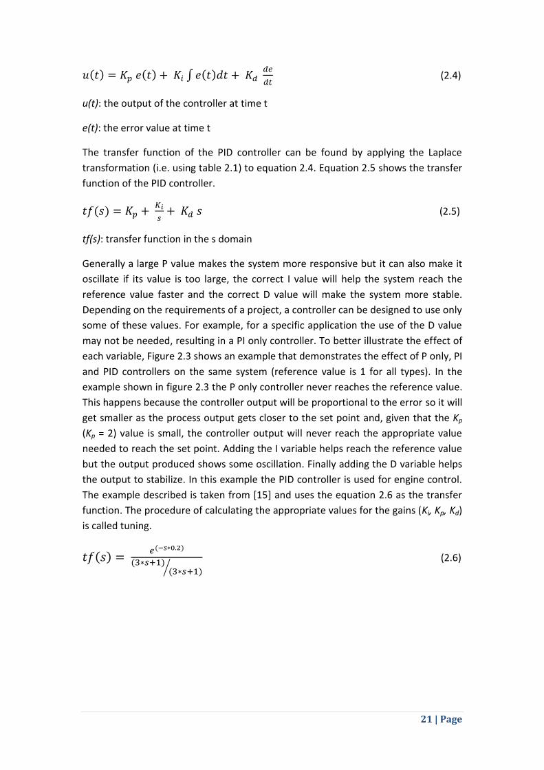
suggest, can be tuned using 3 variables P, I and D. These 3 values are then added to
provide the process input. Figure 2.2 shows the structure of a PID controller.
The P value compensates for the present error and is just a multiplication of the
proportional gain Kp multiplied by e(t) (error on time t). The I value compensates for
the errors in the past, is calculated by multiplying the internal gain Ki and the
integration of e(t). The D value is a prediction for errors in the future, based on the
current rate of errors and is calculated by multiplying the derivative gain Kd and the
differentiation of e(t). The equation 2.4 shows the typical PID equation.
Figure 2.2, PID control scheme, r(t) is the reference value at time t, e(t) is the
error value at time t, u(t) is the output of the controller (input of the process) at
time t and y(t) is the output of the system at time t, from ref [14]
21 | Page
(2.4)
u(t): the output of the controller at time t
e(t): the error value at time t
The transfer function of the PID controller can be found by applying the Laplace
transformation (i.e. using table 2.1) to equation 2.4. Equation 2.5 shows the transfer
function of the PID controller.
(2.5)
tf(s): transfer function in the s domain
Generally a large P value makes the system more responsive but it can also make it
oscillate if its value is too large, the correct I value will help the system reach the
reference value faster and the correct D value will make the system more stable.
Depending on the requirements of a project, a controller can be designed to use only
some of these values. For example, for a specific application the use of the D value
may not be needed, resulting in a PI only controller. To better illustrate the effect of
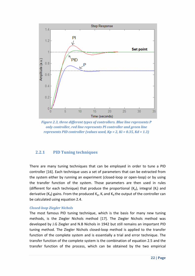
each variable, Figure 2.3 shows an example that demonstrates the effect of P only, PI
and PID controllers on the same system (reference value is 1 for all types). In the
example shown in figure 2.3 the P only controller never reaches the reference value.
This happens because the controller output will be proportional to the error so it will
get smaller as the process output gets closer to the set point and, given that the Kp
(Kp = 2) value is small, the controller output will never reach the appropriate value
needed to reach the set point. Adding the I variable helps reach the reference value
but the output produced shows some oscillation. Finally adding the D variable helps
the output to stabilize. In this example the PID controller is used for engine control.
The example described is taken from [15] and uses the equation 2.6 as the transfer
function. The procedure of calculating the appropriate values for the gains (Ki, Kp, Kd)
is called tuning.
(2.6)
22 | Page
2.2.1 PID Tuning techniques
There are many tuning techniques that can be employed in order to tune a PID
controller [16]. Each technique uses a set of parameters that can be extracted from
the system either by running an experiment (closed-loop or open-loop) or by using
the transfer function of the system. Those parameters are then used in rules
(different for each technique) that produce the proportional (Kp), integral (Ki) and
derivative (Kd) gains. From the produced Kp, Ki and Kd the output of the controller can
be calculated using equation 2.4.
Closed-loop Ziegler Nichols
The most famous PID tuning technique, which is the basis for many new tuning
methods, is the Ziegler Nichols method [17]. The Ziegler Nichols method was
developed by J.G Ziegler and N.B Nichols in 1942 but still remains an important PID
tuning method. The Ziegler Nichols closed-loop method is applied to the transfer
function of the complete system and is essentially a trial and error technique. The
transfer function of the complete system is the combination of equation 2.5 and the
transfer function of the process, which can be obtained by the two empirical
Figure 2.3, three different types of controllers. Blue line represents P
only controller, red line represents PI controller and green line
represents PID controller (values used, Kp = 2, Ki = 0.35, Kd = 1.3)
23 | Page
methods mentioned in section 2.1.1. To tune a controller using the Ziegler Nichols
method this procedure is followed:
i) Kp in the equation 2.5 is set to a value close to zero and Ki and Kd are
turned off completely (set to zero).
ii) The Kp value is increased until the output of the control loop is steadily
oscillating. Ku is equal to the Kp used to produce steady oscillation.
iii) The period of the steady oscillation Pu is then measured.
iv) Using the table 2.3 the values for τΙ and τD can be calculated (Kp, Ki and Kd
can be produced from the τ values, Kp = Kc, Ki = Kc / τi, Kd = Kc * τd).
The closed-loop Ziegler Nichols method is best suited to high order systems (i.e.
systems that their transfer function is cubic or of a higher degree) or systems with
time delay.
Open-loop Ziegler Nichols
Similarly to the closed-loop technique the open-loop Ziegler Nichols [17] got its
name from its inventors. However, unlike the closed-loop method this technique is
applied directly to the process and does not involve any feedback hence is an open-
loop method. The procedure followed is the same as the one used to retrieve the
transfer function of the process using a step response (sections 2.1.1 and 3.3.1).
Using the parameters K, T and L from equation 2.2 and table 2.4, Kp, Ki and Kd can be
produced. The open-loop Ziegler Nichols can be used with every type of system.
Table 2.3, closed –loop Ziegler Nichols PID tuning
chart, from ref [18]
24 | Page
Controller Kc τi τD
P
- -
PI
-
PID
2 * L 0.5 * L
Ziegler Nichols is the most famous technique but there are also many other
techniques available. Other often used techniques include Cohen-Coon (open-loop)
[19], Tyreus-Luyben (closed-loop) [20], Internal Model Control (IMC) [21], etc. An
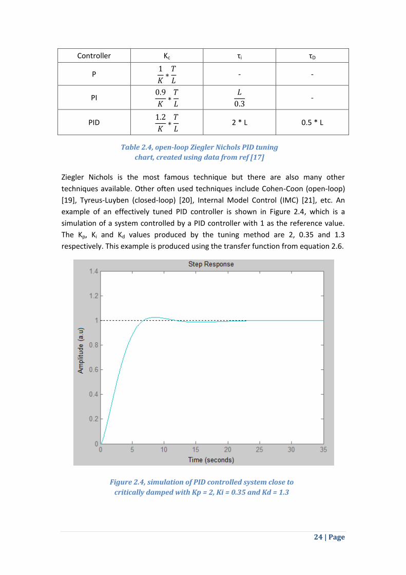
example of an effectively tuned PID controller is shown in Figure 2.4, which is a
simulation of a system controlled by a PID controller with 1 as the reference value.
The Kp, Ki and Kd values produced by the tuning method are 2, 0.35 and 1.3
respectively. This example is produced using the transfer function from equation 2.6.
Figure 2.4, simulation of PID controlled system close to
critically damped with Kp = 2, Ki = 0.35 and Kd = 1.3
Table 2.4, open-loop Ziegler Nichols PID tuning
chart, created using data from ref [17]

25 | Page
2.3 Hardware components and software tools
In this project, the Raspberry Pi platform is used to incorporate the PID controller
software and communicate with hardware components. Raspberry Pi is used in
combination with additional standard, off the shelf hardware components to form
the complete system. The input and output resolution of those hardware
components is an important characteristic that was taken under consideration for
the selection of the components. Finally, the logic of the controller was implemented
using the Python programming language. This section includes details about these
topics.
2.3.1 Raspberry Pi
Raspberry Pi [1] is a credit-card sized computer developed by the Raspberry Pi
Foundation in the United Kingdom. Raspberry Pi has 2 different models. Both models
use the same SoC (System on Chip), which contains an ARM11 processor [22]. In this
project, a model B is used which has 512 MB RAM (model A has 256 MB) and two
USB ports (model A has one). Raspberry Pi can run several Linux distributions
through an SD card. For this project Raspbian [23] was used.
Raspberry Pi supports a variety of programming languages. For this project, the main
programming language of Raspberry Pi will be used, which is Python. Python was
selected because is the most supported language in terms of modules for GPIO
(General Purpose Input Output).
Raspberry Pi can be used as a personal computer, as well as a microcontroller. In this
project Raspberry Pi is used as a microcontroller. Raspberry Pi has 26 pins, 17 of
them can be used as GPIO (general purpose input output) pins. Those pins are
programmable using software and can be used to start or stop a device. GPIOs can
only provide voltage of 0V or 3.3V (low or high). Figure 2.5 shows a picture of
Raspberry Pi and its pins. Generally GPIOs are used for communication between the
Raspberry Pi and other devices.

26 | Page
2.3.2 Python programming language
Python [24] is a programming language designed by Guido van Rossum that first
appeared in 1991. Python is a high-level language, developed under an open-source
license, making it freely usable and distributable. Today, Python is widely used in
many applications. Some of its many usages are web and internet development,
database interfacing, game development, graphical interfaces and scientific
applications. Furthermore, Python can also be used to replace much functionality of
proprietary tools such as MATLAB [30], in the area of control systems and
mathematics. The latest version of Python is 3.4, released on March 16, 2014.
Python supports both object-oriented programming and structural programming.
The major Python implementations use a compiler to translate the source code to
byte code which is then run using a virtual machine. One of the strengths of Python
is that its syntax allows few lines of code to carry the same functionality as larger
pieces of code written in other languages. Another special characteristic of Python is
the requirement of indentation in the code to denote blocks of code, e.g. if-else code
block.
Libraries in Python come in the form of modules, which need to be installed in the
environment before they are used. Some popular modules that are used in this
project are SciPy[25] (mathematics and generally scientific functionality),
RPi.GPIO[26] (interface to Raspberry Pi GPIOs), python-control[27] (control system
functionality) and matplotlib [28] (port of several functions from MATLAB).
Figure 2.5, Raspberry Pi, highlighted with the red rectangle are the 26 pins
27 | Page
2.3.3 Input and output resolution
An important criterion that was taken under consideration when selecting the
standard, off the shelf hardware components was input and output resolution. The
term resolution regarding the input from a sensor and the output to a device is
closely related to the precision of the value received or provided. Resolution may be
defined in bits. For example, to set the speed of a fan in a setting other than full
speed it is needed to provide a digital value that represents voltage ranging from 0
to 2n - 1 where n is the number of bits or the resolution. So if it is determined that
the resolution is 8 bits then the digital values that represent voltage range from 0 to
255, thus to set the fan at e.g. 80% speed the digital value that represents voltage
should be set to 205. This is an example of output resolution. Input resolution works
in a similar way. For example, a temperature sensor that provides a 10 bit input
produces a digital value representing measured voltage between 0 and 1023, which
will then translate to a specific temperature in degrees Celsius. In both cases, the
higher the resolution (the number of bits) the better the precision. This is a result of
having more distinct digital values. A 16 bit resolution results in 65536 different
values which can then be translated to a reading, e.g. temperature, speed, etc. In
contrast, an 8 bit resolution results in only 256 values. To better illustrate this, it is
assumed that digital value 180 is received as the measured voltage from an 8 bit
temperature sensor, which for instance equals to 23.5 oC. Assume that a cooler
should be started when the temperature is exactly 23.75 oC, so the next readings
should be checked to see if the temperature has reached that point. The next digital
voltage number received is 181 which, for instance, translates to 24 oC (for a
common sensor, an 8 bit resolution usually translates to a resolution of 0.5 oC or
higher for every step in the digital value). In this case the cooler will never start as a
step of 1 in the digital voltage value results to a 0.5 step in degrees Celsius so the
resolution is not enough to measure up to the second digit and the temperature
reading will never reach 23.75 oC. This problem can be solved by using a higher
resolution as having more possible distinct values will reduce the difference in
degrees for a step of 1 in the digital voltage value.
The use of Digital to Analogue Converters (DAC) and Analogue to Digital Converters
(ADC) is essential to translate voltage to and from a continuously varying value e.g.
temperature. DAC is used to output a voltage from the microcontroller in order to
power a device. ADC is used to input voltage to the microcontroller in order to
measure the output of a device. The resolution discussed above is used to describe
the precision of these converters.
28 | Page
3. Design and Methodology for PID Controllers
In this chapter, the design decisions and the methodology followed to develop the
PID controller are described.
The first section contains information about the methodology followed throughout
the project. The project is divided to individual parts and the required work for each
part is described.
The second section contains two block diagrams of the system. The first block
diagram shows the components used in the analysis of the controller. From this
diagram the transfer function for the complete closed-loop system can be produced.
The second block diagram shows the same system but using hardware components.
The third section includes information about the two selected system identification
techniques, step response and parameter estimation. For both system identification
techniques the complete procedure is described, from the initial experiment to the
transfer function model construction.
The forth section contains information about the PID tuning technique selection. It is
discussed why the specific technique is selected and what benefits it offers to the
system.
3.1 Methodology
This project consists of three major parts that need to be implemented. The three
parts are: i) input, ii) controller logic, iii) output. Figure 3.1 shows how these three
parts are connected.
Figure 3.1. The three parts of the project (Input, Controller,
Output), their connection and the connection between them
and various devices and sensors.
29 | Page
Initially, most effort was devoted on the input and output parts. Those parts
included the most hardware related work. Input is related to the method used to
read the data provided by the sensors and transform it in a form that the controller
can use. Challenges related to input include the resolution that should be used, the
translation of the input (usually in voltage) to a form that the controller can use (e.g.
temperature) and the identification of suitable hardware components. Output is
related to the method used to provide data from the controller to various devices
(e.g. a fan, a heater) and its transformation in a form that devices can use (e.g.
voltage or current). Challenges related to output are similar to those related to
input. Resolution, translation of data to voltage and selection of suitable hardware
components are the main challenges.
After work on the input and output side was completed the controller design and
implementation started. The controller part involved more software coding.
Decisions were made on what system identification method to use and how to
implement it, what tuning technique to use, what tools and libraries can be used and
the type of simulations and experiments that will be used to evaluate the system.
The procedure started with the design of block diagrams and running some
simulations using the Simulink [29] tool.
3.2 System block diagram
A block diagram represents the individual components of the system and the
connection between them. Using the block diagram one can identify what is the
input and what is the output of each individual component. A block diagram can also
be used to derive the closed-loop transfer function of the system. Figure 3.2 shows
the block diagram designed for the system that was built (using a set point of 1). The
block diagram was designed using the Simulink tool [29] of MATLAB [30].
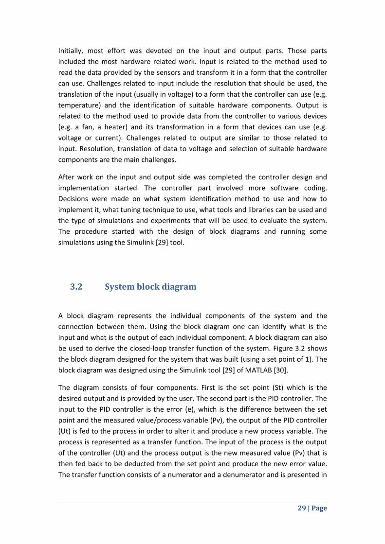
The diagram consists of four components. First is the set point (St) which is the
desired output and is provided by the user. The second part is the PID controller. The
input to the PID controller is the error (e), which is the difference between the set
point and the measured value/process variable (Pv), the output of the PID controller
(Ut) is fed to the process in order to alter it and produce a new process variable. The
process is represented as a transfer function. The input of the process is the output
of the controller (Ut) and the process output is the new measured value (Pv) that is
then fed back to be deducted from the set point and produce the new error value.
The transfer function consists of a numerator and a denumerator and is presented in
30 | Page
the s-domain. Finally the last component is the Scope which is the hardware that is
used to view the closed-loop output.
In addition, the block diagram can help to identify the closed-loop transfer function
of the complete system. As the block diagram is presented in the s-domain the
transfer function can be identified by combining consecutive components of the
system [9]. For this system the PID controller transfer function is represented by Gc
and the process transfer function is represented by Gp. Therefore the closed-loop
transfer function of the complete system, based on equation 2.1, is given by
equation 3.1.
(3.1)
Gs : closed-loop transfer function of the system
Gc: transfer function of the controller
Gp: transfer function of the process
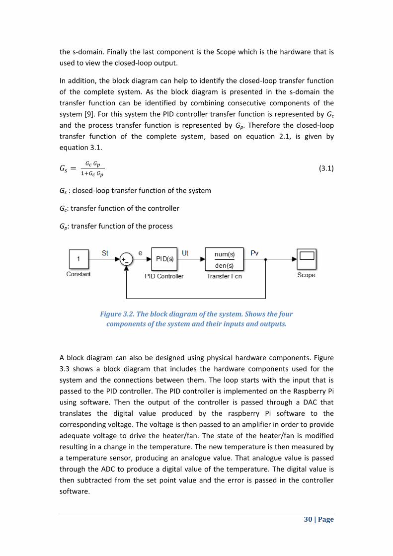
A block diagram can also be designed using physical hardware components. Figure
3.3 shows a block diagram that includes the hardware components used for the
system and the connections between them. The loop starts with the input that is
passed to the PID controller. The PID controller is implemented on the Raspberry Pi
using software. Then the output of the controller is passed through a DAC that
translates the digital value produced by the raspberry Pi software to the
corresponding voltage. The voltage is then passed to an amplifier in order to provide
adequate voltage to drive the heater/fan. The state of the heater/fan is modified
resulting in a change in the temperature. The new temperature is then measured by
a temperature sensor, producing an analogue value. That analogue value is passed
through the ADC to produce a digital value of the temperature. The digital value is
then subtracted from the set point value and the error is passed in the controller
software.
Figure 3.2. The block diagram of the system. Shows the four
components of the system and their inputs and outputs.
31 | Page
3.3 System identification methods
To obtain the model of a process an empirical method can be used. Typically an
empirical method involves of an input to the process, step or random, and the
extraction of the characteristics of the process based on the output. Using those
characteristics a transfer function can be formed. Step response and parameter
estimation system identification techniques are both implemented in order to
evaluate which one produces better results.
3.3.1 Step response
As stated in section 2.1.1 a process transfer function can be obtained by an open-
loop experiment with a step in the input of the process. The procedure of modelling
a process using the step response method starts with the system at rest. Then an
open-loop experiment is performed. The process input/controller output is stepped
to a larger value and the process output is measured and stored. The data is then
plotted. From the plot, characteristics of the process can be retrieved and fitted in
the three parameter equation 3.2 to produce the transfer function of the process.
There are different methods that can be used to calculate the values of time
constant T and time delay L.
(3.2)
K: static gain
T: time constant
Figure 3.3. The block diagram of the temperature control
system. Shows the hardware components of the system.

32 | Page
L: dead time or time delay
K, T and L can be described in words as:
K shows how much the process output will change for a given process input.
For example, for a temperature control system, where the input is measured
as a percentage of power and output is measured in degrees Celsius, K is
equal to 0.5 oC/%. This means that for a step of 1% in the input the process
output will be increased by 0.5 oC.
T shows how fast the process responds after a change in the process input. T
is always expressed in time units (seconds or minutes).
L shows how much time it takes the process to start responding after a
change in the process input. For example, if the time delay L is equal to 2
minutes and a process input is applied at 10:00 then the process output will
start changing at 10:02.
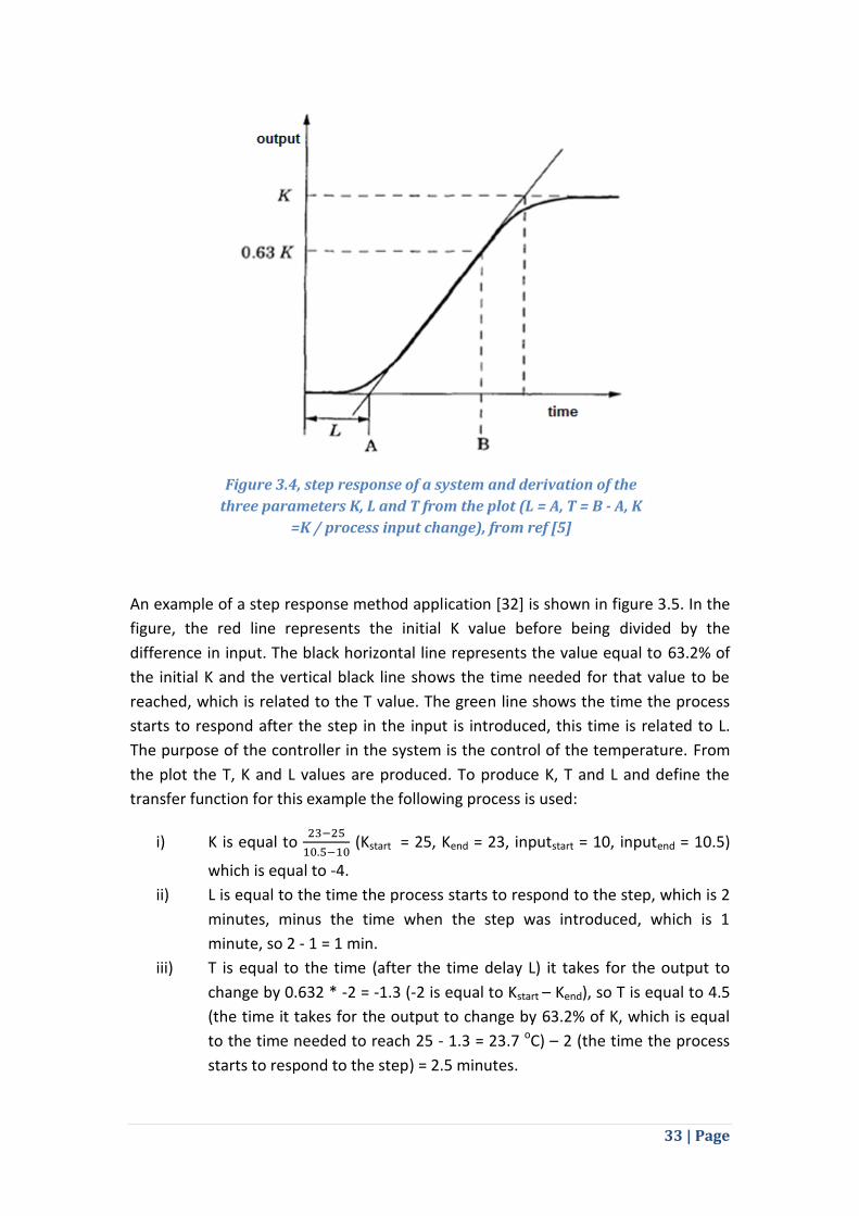
3.3.1.1 63.2% and Tangent Method
The 63.2% and tangent method is the most common technique used for forming a
transfer function using a step response. The value 63.2% is derived from equation
3.3 [31], which relates the output of a step response with the final steady-state
output value.
(3.3)
KΔu: the final steady-state output value
T: the time constant
After one time constant (t = T) the response is equal to 1 – e-1 which is equal to
0.632. Using this method K is derived from the final steady-state gain divided by the
change in the process input/controller output. L is derived by drawing a tangent
along the inflection point of the curve (the point the curve starts changing direction)
and taking the point where the line intersects the x-axis or the time needed for the
process output to change significantly. T is equal to the time (after the time delay)
where the value equal to 63.2% of K was reached. Figure 3.4 shows this procedure
graphically. An advantage of this method is that parameters can be easily
approximated by just inspecting the plot. However, one drawback of this method is
its sensitivity to noise as it depends on individual points on the curve.
33 | Page
An example of a step response method application [32] is shown in figure 3.5. In the
figure, the red line represents the initial K value before being divided by the
difference in input. The black horizontal line represents the value equal to 63.2% of
the initial K and the vertical black line shows the time needed for that value to be
reached, which is related to the T value. The green line shows the time the process
starts to respond after the step in the input is introduced, this time is related to L.
The purpose of the controller in the system is the control of the temperature. From
the plot the T, K and L values are produced. To produce K, T and L and define the
transfer function for this example the following process is used:
i) K is equal to
(Kstart = 25, Kend = 23, inputstart = 10, inputend = 10.5)
which is equal to -4.
ii) L is equal to the time the process starts to respond to the step, which is 2
minutes, minus the time when the step was introduced, which is 1
minute, so 2 - 1 = 1 min.
iii) T is equal to the time (after the time delay L) it takes for the output to
change by 0.632 * -2 = -1.3 (-2 is equal to Kstart – Kend), so T is equal to 4.5
(the time it takes for the output to change by 63.2% of K, which is equal
to the time needed to reach 25 - 1.3 = 23.7 oC) – 2 (the time the process
starts to respond to the step) = 2.5 minutes.
Figure 3.4, step response of a system and derivation of the
three parameters K, L and T from the plot (L = A, T = B - A, K
=K / process input change), from ref [5]

34 | Page
Therefore, using the 2.2 equation, the transfer function of the process is:
3.3.1.2 Method of Moments
Method of moments [33] uses integration to estimate T and L by calculating the area
between the curve of the plotted output and the two axes. Figure 3.6 shows an
example of the areas that need to be calculated. A1 is the area between the output
curve and the y-axis and A2 is the area between the output curve and the x-axis. K
can be calculated the same way as in the previous method, the division of the
difference in the output and the difference in the input. Using A1 and K, L + T can be
calculated. Equation 3.4 gives L + T.
(3.4)
Figure 3.5, example of step response of a system. a) Shows the output of the
system. Dashed line is the smoothened step response output, solid line is the
output measurement with noise. b) Shows the process input/controller output
setting during the same time (change between 10 and 10.5 represents the step),
from ref [32]

35 | Page
Then the area between the output curve and x-axis, starting from time t0 (time that
the step in the input is applied) until time L + T gives A2. Equation 3.5 shows how A2
is calculated.
(3.5)
y0 represents the output of the system when the system is on its initial steady-state
(before time t0). y(t) – y0 is used to calculate the deviation of the measured output
from the steady-state output, it is a deviation variable. Finally, using equations 3.6
and 3.7 T and L can be calculated.
(3.6)
(3.7)
Method of moments has the advantage of being more tolerant to noise than any
point specific technique (e.g. point in time of 63.2% of maximum output). The
method of moments does not depend on only one point so noise in the process
output will have less of an effect on this method.
3.3.1.3 2-point method
The 2-point method [34] is similar to the 63.2% method but instead of relying on
only a single point it relies on two distinct points. The two points that are used on
Figure 3.6. The calculation of gain K, time constant T and
time delay L using the method of moments, from ref [33]
36 | Page
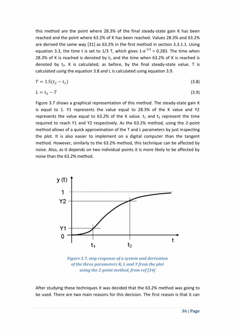
this method are the point where 28.3% of the final steady-state gain K has been
reached and the point where 63.2% of K has been reached. Values 28.3% and 63.2%
are derived the same way [31] as 63.2% in the first method in section 3.3.1.1. Using
equation 3.3, the time t is set to 1/3 T, which gives 1-e-1/3 = 0.283. The time when
28.3% of K is reached is denoted by t1 and the time when 63.2% of K is reached is
denoted by t2. K is calculated, as before, by the final steady-state value. T is
calculated using the equation 3.8 and L is calculated using equation 3.9.
(3.8)
(3.9)
Figure 3.7 shows a graphical representation of this method. The steady-state gain K
is equal to 1. Y1 represents the value equal to 28.3% of the K value and Y2
represents the value equal to 63.2% of the K value. t1 and t2 represent the time
required to reach Y1 and Y2 respectively. As the 63.2% method, using the 2-point
method allows of a quick approximation of the T and L parameters by just inspecting
the plot. It is also easier to implement on a digital computer than the tangent
method. However, similarly to the 63.2% method, this technique can be affected by
noise. Also, as it depends on two individual points it is more likely to be affected by
noise than the 63.2% method.
After studying these techniques it was decided that the 63.2% method was going to
be used. There are two main reasons for this decision. The first reason is that it can
Figure 3.7, step response of a system and derivation
of the three parameters K, L and T from the plot
using the 2-point method, from ref [34]

37 | Page
be easier and more accurately implemented in a digital computer. The second one is
that the results of the 63.2% can be evaluated by just analysing the output plot.
3.3.2 Parameter Estimation
As the step response method, parameter estimation [35] is a technique that uses an
input to the system to produce an output that can be processed in order to form the
transfer function of the process. Figure 3.8 shows the process. Most of the equations
in this section and its subsections are taken from [36] and are used to demonstrate
how parameter estimation can be used to obtain the transfer function.
In contrast to the step response method, in parameter estimation the input is not a
step in the value of the process input/controller output, but instead is a random
selection between two possible numbers. The input is usually generated using a
Pseudorandom Binary Sequence (PRBS). Following the input, the process responds
and its output is used to generate a transfer function in the form of equation 3.10.
(3.10)
a1, a2, b1, b2: parameters estimated by the output
In parameter estimation the output of the system is represented using equations
3.11 – 3.13. These three equations show the different ways that the output can be
represented (i.e. 3.11 can be reformed as 3.12 or 3.13 and vice versa).
(3.11)
Figure 3.8. General representation of the parameter estimation
method. Input and output are used to produce the parameter
vector and therefore the transfer function, from ref [36]
38 | Page
(3.12)
(3.13)
y and φ are produced using data from the PRBS experiment. y is a known vector
consisting of measured outputs from the PRBS experiment, φ is a known matrix
consisting of input and output from the PRBS experiment and θ is the unknown
vector that should be found in order to form the transfer function. For example, ym
represents the mth measured output in the PRBS experiment. As y, φ and θ involve
vectors the equation 3.13 can also be written as equation 3.14 and 3.15. Also, as
shown in equation 3.16, θ is used to identify the a1, a2, b1 and b2 values used to form
the transfer function in equation 3.10.
(3.14)
(3.15)
(3.16)
To find θ the least squares (LS) method can be used.
3.3.2.1 Pseudorandom Binary Signal (PRBS)
Pseudorandom Binary Sequence [36] is a sequence of values that can be used as the
input to the process in the parameter estimation system identification technique. A
pseudorandom binary signal can only contain two possible values, e.g. 0 and 1. The
procedure of generating a PRBS starts by selecting the two possible values and a
probability p. Probability p should be small enough so that the value does not change
too frequently in order to allow time for the process to respond (p = 0.1 is a
frequently used value). One of the two possible values is selected as the initial value
and is appended in the empty sequence. Following that, a random number between
0.0 and 1.0 is generated. If that number is smaller than the probability p the value
switches from the previous value to the other possible value and that value is
appended to the sequence. The same procedure continues and the value only
switches if the random number is smaller than the probability p. Using PRBS,
information of how the process reacts on sudden and steep changes in the process
input can be extracted. Figure 3.9 shows an example of a PRBS signal with 1 and -1 as
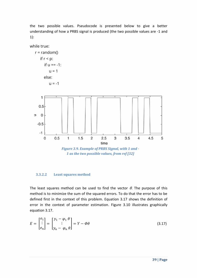
39 | Page
the two possible values. Pseudocode is presented below to give a better
understanding of how a PRBS signal is produced (the two possible values are -1 and
1):
while true:
r = random()
if r < p:
if u == -1:
u = 1
else:
u = -1
3.3.2.2 Least squares method
The least squares method can be used to find the vector θ. The purpose of this
method is to minimize the sum of the squared errors. To do that the error has to be
defined first in the context of this problem. Equation 3.17 shows the definition of
error in the context of parameter estimation. Figure 3.10 illustrates graphically
equation 3.17.
(3.17)
Figure 3.9. Example of PRBS Signal, with 1 and -
1 as the two possible values, from ref [32]
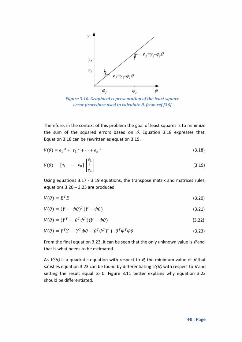
40 | Page
Therefore, in the context of this problem the goal of least squares is to minimize
the sum of the squared errors based on θ. Equation 3.18 expresses that.
Equation 3.18 can be rewritten as equation 3.19.
(3.18)
(3.19)
Using equations 3.17 - 3.19 equations, the transpose matrix and matrices rules,
equations 3.20 – 3.23 are produced.
(3.20)
(3.21)
(3.22)
(3.23)
From the final equation 3.23, it can be seen that the only unknown value is θ and
that is what needs to be estimated.
As V θ is a quadratic equation with respect to θ, the minimum value of θ that
satisfies equation 3.23 can be found by differentiating V θ with respect to θ and
setting the result equal to 0. Figure 3.11 better explains why equation 3.23
should be differentiated.
Figure 3.10. Graphical representation of the least square
error procedure used to calculate θ, from ref [36]
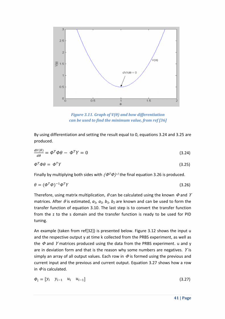
41 | Page
By using differentiation and setting the result equal to 0, equations 3.24 and 3.25 are
produced.
(3.24)
(3.25)
Finally by multiplying both sides with ΦTΦ -1 the final equation 3.26 is produced.
(3.26)
Therefore, using matrix multiplication, θ can be calculated using the known Φ and Υ
matrices. After θ is estimated, a1, a2, b1, b2 are known and can be used to form the
transfer function of equation 3.10. The last step is to convert the transfer function
from the z to the s domain and the transfer function is ready to be used for PID
tuning.
An example (taken from ref[32]) is presented below. Figure 3.12 shows the input u
and the respective output y at time k collected from the PRBS experiment, as well as
the Φ and Υ matrices produced using the data from the PRBS experiment. u and y
are in deviation form and that is the reason why some numbers are negatives. Υ is
simply an array of all output values. Each row in Φ is formed using the previous and
current input and the previous and current output. Equation 3.27 shows how a row
in Φ is calculated.
(3.27)
Figure 3.11. Graph of V(θ) and how differentiation
can be used to find the minimum value, from ref [36]

42 | Page
Then using equation 3.26, θ is calculated. The result is:
Using equation 3.16, a1 = -1.1196, a2 = 0.3133, b1 = -0.0889, b2 = 0.2021. Then by
fitting these values to the equation 3.10, the transfer function is produced (equation
3.28).
(3.28)
Finally, transforming this transfer function to the s-domain gives the final transfer
function of the process (equation 3.29) that can be used for PID tuning.
(3.29)
Figure 3.12. First table contains input and output data in
deviation form at discrete time k, second table is the Φ matrix and
third table is the Y matrix, drawn using data taken from ref [32]

43 | Page
3.4 Tuning techniques
The tuning technique that was selected is the open-loop Ziegler-Nichols method.
This method was selected as it is suitable for all the types of systems, in contrast to
the closed-loop method that is better suited to systems of third order or higher (i.e.
systems that their transfer function is cubic or of a higher degree) or with significant
time delay. In addition, using open-loop tuning in conjunction with an empirical
system identification technique allows the controller to control a variety of systems
without modifications in the implementation. This advantage of the open-loop
method is important for the fulfilment of the additional deliverable, building a
flexible system that has the ability to control a variety of systems. If closed-loop
Ziegler-Nichols is used, the gains are manually estimated after running a closed-loop
experiment. Although, this is more convenient and less complex to understand and
implement, as it does not require a system identification technique implementation
or an extensive tuning technique implementation, it hinders the flexibility of the
controller. Whenever a different system needs to be controlled a new, manual, trial
and error experiment must be run by someone with knowledge of the closed-loop
experiment procedure. Furthermore, the open-loop method is better suited for a
digital implementation as the closed-loop requires a trial and error procedure.
Open-loop Ziegler-Nichols can be implemented similarly to the step response using
any method described in section 3.3.1. After K, T and L are produced the rules found
on table 2.4 are used to produce the proportional, integral and derivative gains.
44 | Page
4. Implementation for PID Controllers
This chapter contains details about the implementation of the whole system.
The first section describes the procedure of building the system. It also includes the
designs produced for the system. Furthermore, it provides details about the selected
input and output hardware components.
The second section describes how the interfacing between the hardware
components and the Raspberry Pi was achieved. Both interfacing with input and
output hardware is described.
The third section describes the implementation of the PID controller. The
implementation of the PID controller includes the initial experiment and the system
identification for both step response and parameter estimation. The PID controller
tuning and the PID controller loop implementation are also described. Finally, some
additional minor considerations regarding the implementation of a PID controller are
also discussed.
The fourth and final section shows the interface used by the user to operate the
system. It also includes a demonstration of the working system.
4.1 Building the system
To evaluate the actual performance and efficiency of the PID controller, simulations
are not enough. Even though many simulations should be made before actual
evaluations, they do not take into consideration important aspects of the system.
Such aspects include external and unexpected disturbances, noise, limitations of the
actual hardware components, etc. Therefore, in order to get a clear picture of the
performance of the PID controller an actual evaluation system must be built.
Initially there were two types of systems under consideration. The first one included
a fan, whose speed will be controlled by the DAC based on the output of the
controller. The fan will regulate the temperature of an enclosed environment, e.g.
some kind of a box, by bringing air from the outside environment. The temperature
sensor will be positioned inside the enclosed environment and provide

45 | Page
measurements to the controller in order to speed up or down the fan. The second
system included two cartridge heaters mounted onto an aluminium block. The
cartridge heaters were connected in series and controlled by the DAC (through an
external power supply) after the output of the controller. The temperature sensor
was connected to the aluminium block in order to monitor the temperature of the
block and notify the controller. The controller will then provide more or less power
to the heaters accordingly.
From these two systems the system with the aluminium block and the cartridge
heaters was selected. The advantages of this system over the first system are:
i) The range of temperature control is greater than the first system, which
depends greatly on the room temperature.
ii) Is more tolerant to noise and is not affected as much by disturbances as the
first system.
The disadvantages of this system compared to the first system are:
i) There will be a bigger delay between the output of the DAC and the actual
rise or drop in temperature, due to the time it takes for heat to transfer in
the aluminium block, making the system more challenging to control.
ii) An external power supply is needed as the heaters require 24 V and the
raspberry pi can provide at most 5 V.
The advantages were considered to outweigh the disadvantages, so the heaters
system was selected. The ability to control the system over a larger range of
temperatures without a lot of noise was considered important in order to validate
the competence of the controller.
After the selection of the system, the required components were assembled. First of
all, the aluminium block was designed. Figure 4.1 shows the design of the aluminium
block.

46 | Page
The block has a 50.8 mm (2 inch) diameter and is 25.4 mm (1 inch) tall. It also has
four flat edges, 2 mm deep each, these edges are used to attach the temperature
sensor directly to the block. Finally, one of the edges also has two holes cut into it,
each is 25 mm deep with a 6.25 mm radius. These two holes are used to attach the
cartridge heaters into the block. The design was then given to the workshop and the
block was produced. After the construction of the first aluminium block, the need for
some additional holes to hold the temperature sensor in place was identified. The
second aluminium block constructed had four small additional holes in each of the
four flat sides. The holes were designed for M3 screws and an additional small
horizontal aluminium piece with two same sized holes was created. The holes and
the additional piece allowed the temperature sensor to be held firmly in place and
also allowed the positioning of the sensor to change in all of the four flat edges.
Figure 4.1. Design of the aluminium block. View of the whole
block, front view showing the holes, top view showing the cuts
and top view showing the holes. All dimensions are in mm.
47 | Page
4.1.1 Hardware components
As described in the previous section, in this project an ADC, a DAC, a temperature
control and a heater are the main hardware parts.
The temperature sensor used is a SHT71 manufactured by Sensirion [37]. This sensor
provides temperature and humidity measurements. It is fully calibrated and uses a
two-wire interface (clock and data) for communication with the Raspberry Pi. It also
has an integrated ADC that provides a 16 bit output from which 14 bits are used. The
14 bit resolution translates to a resolution of 0.01 oC. The sensor also offers a
response time of 5 seconds, which is considered relatively fast.
When it comes to temperature sensors, usually there is a trade-off between
response time and accuracy. For example, sensors with response time of 2.5-3.5
seconds or even faster are available but they are not as accurate. On the other hand,
even more accurate sensors are available but there response time can reach up to 1
minute. The SHT71 sensor offers balance between speed and accuracy. Relatively to
the evaluation system described in the previous section, this sensor is an appropriate
choice because:
The high resolution should help the performance of the PID controller, as the
more precise the measurement is the more precise the controller output will
be.
The temperature systems that this controller is intended to be used with do
not operate in a very large range of temperatures so accuracy is needed.
Furthermore, the high resolution enhances the flexibility of the controller as
it can be used to control temperature systems where precision in small
temperature changes is important.
Heat coming out of the heaters in the aluminium block requires some time
to reach the temperature sensor. In addition to that, temperatures in the
evaluation system or systems that depend on room temperature do not tend
to increase by a large margin rapidly. As a result, the time constant of the
system is expected to be larger than 5 seconds, therefore a response time of
5 seconds should be adequate.
The ADC used is an ADS1115 implementation by Adafruit [38]. The purpose of an
ADC is to transform analogue voltage signal into digital data. For example, an ADC
can be used to translate the temperature provided by a temperature sensor to a
digital value that Raspberry Pi can use. Raspberry Pi does not have an integrated
ADC, therefore an external ADC is required to translate analogue data to digital. The
chosen ADC was selected mainly because of its resolution of 16 bit as well as its low
cost.
48 | Page
The DAC used is an AD5662 manufactured by Analogue Devices [39]. The purpose of
a DAC is to translate a digital value to an analogue one (voltage). Through each GPIO
pin, Raspberry Pi can only pass full voltage (1 or HIGH) or zero voltage (0 or LOW).
Using the DAC, voltage between 0V and 3.3V can be provided. The digital value is
provided by the Raspberry Pi to the DAC and it is then translated to voltage that is
outputted by the DAC. A DAC was selected to power the heaters (through an
external power amplifier) as it provides a stable and accurate output. The DAC
output is used by the external power amplifier as a control voltage to provide the
appropriate power to the heaters. AD5662 was selected mainly because of its 16 bit
resolution and its low cost.
4.2 Interfacing with hardware components
In terms of hardware components, implementation includes both wiring and coding.
This section includes both input (ADC, temperature sensor) and output (LCD screen,
heaters) devices. Both the wiring and interfacing of the devices are described in
detail in the following sections. Circuit and wiring diagrams are also presented
showing how these components are connected with Raspberry Pi. After the
interfacing was completed, each individual hardware component was tested to
ensure that it communicated with Raspberry Pi as expected.
4.2.1 Input devices
The input devices used in this project are an Analogue to Digital Convertor (ADC) and
a temperature sensor. The temperature sensor used is an SHT71 and the ADC used is
an ADS1115.
Temperature sensor
For the temperature sensor, a Python library [40] is provided making it fairly easy to
connect with the Raspberry Pi. The communication between the Raspberry Pi and
the temperature sensor is done using two pins of the senor, the clock and data pin.
The library handles the communication with the sensor. Using the interface of the
library, the temperature and humidity can be retrieved. The sensor has 4 pins,
voltage supply, ground, data and clock, which are assigned to Raspberry Pi pins. Data
and clock are used by the library to get the measurements. Figure 4.2 shows a circuit
diagram for the temperature sensor.

49 | Page
After wiring is completed code must be written to communicate with the library and
receive readings from the temperature sensor. First of all the library must be
imported.
from sht1x.Sht1x import Sht1x as SHT1x
Then a sensor object must be initialized.
sht1x = SHT1x(SENSOR_INPUT, CLK, SHT1x.GPIO_BCM)
SENSOR_INPUT is the GPIO pin number connected to the data pin of the
temperature senor and CLK is the GPIO pin number connected to the clock pin of the
sensor. Finally, the temperature can be read by calling the appropriate method from
the sensor object.
temperature = sht1x.read_temperature_C()
The object also includes methods for reading humidity and dew point. Figure 4.3
shows how the temperature sensor is wired to the Raspberry Pi.
Figure 4.2. Circuit diagram of the connection
between the sensor and Raspberry Pi, from ref [37]
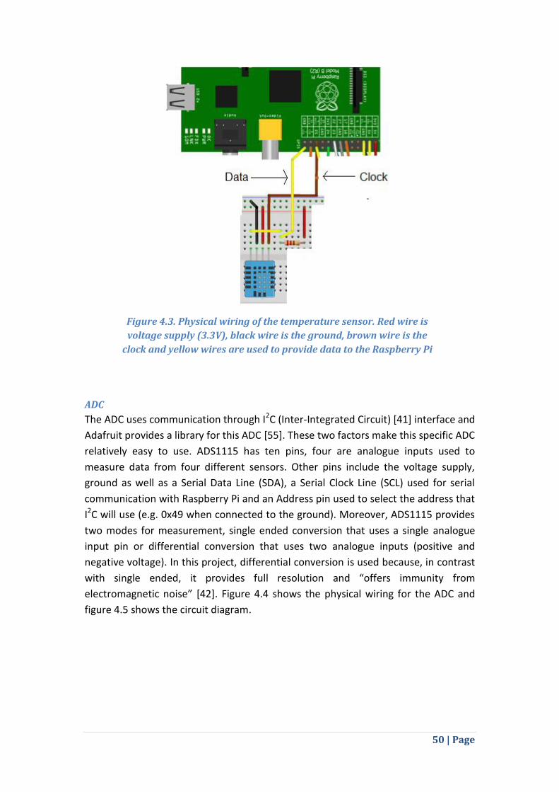
50 | Page
ADC
The ADC uses communication through I2C (Inter-Integrated Circuit) [41] interface and
Adafruit provides a library for this ADC [55]. These two factors make this specific ADC
relatively easy to use. ADS1115 has ten pins, four are analogue inputs used to
measure data from four different sensors. Other pins include the voltage supply,
ground as well as a Serial Data Line (SDA), a Serial Clock Line (SCL) used for serial
communication with Raspberry Pi and an Address pin used to select the address that
I2C will use (e.g. 0x49 when connected to the ground). Moreover, ADS1115 provides
two modes for measurement, single ended conversion that uses a single analogue
input pin or differential conversion that uses two analogue inputs (positive and
negative voltage). In this project, differential conversion is used because, in contrast
with single ended, it provides full resolution and “offers immunity from
electromagnetic noise” [42]. Figure 4.4 shows the physical wiring for the ADC and
figure 4.5 shows the circuit diagram.
Figure 4.3. Physical wiring of the temperature sensor. Red wire is
voltage supply (3.3V), black wire is the ground, brown wire is the
clock and yellow wires are used to provide data to the Raspberry Pi

51 | Page
After wiring is completed, code must be written to communicate with the library and
receive digital values from the ADC. First of all the library must be imported.
from Adafruit_ADS1x15 import ADS1x15
Then an instance of the ADS1x15 class must be created.
adc = ADS1x15(ic=ADS1115) # Create instance of the class ADS1x15
called adc
ic = ADS1115 indicates the model of the ADC. After that the adc is set on continuous
differential conversion.
adc.startContinuousDifferentialConversion(0,1, pga, sps)
Figure 4.4. Physical wiring of ADC. Red wire is voltage
supply (3.3V), black wire is ground, yellow wires are SDA
and SCL and grey wire is used to give I2C address (0x49).
Figure 4.5. ADC circuit diagram. A0 – A4 of the ADC are
connected to the analogue source.

52 | Page
The first two parameters are used to indicate the two analogue inputs compared to
produce the differential output. pga is used to indicate the voltage range measured
by the ADC and sps indicates the samples per second taken by the adc.
Finally, the last conversion (a voltage digital number) is retrieved from the ADC.
adc.getLastConversionResults()
Using the system described in section 4.1 the ADC was not used because the
temperature sensor selected already has an integrated ADC. However, the ADC
interface implementation was done before the design of the evaluation system, so
although it was not used in this system, the implementation can be used as part of
the additional deliverable, which is to design a flexible controller able to control a
variety of systems. With the ADC implementation additional sensors without an
integrated ADC can be connected with Raspberry Pi.
4.2.2 Output devices
The output devices used in this project are a Digital to Analogue Convertor (DAC), an
LCD screen and two heaters. The DAC used is an AD5662, the screen is an LCD of
16x2 characters and the heaters are standard 24V cartridge heaters.
DAC
Unfortunately, there is no library for the selected DAC so the code had to be written
from scratch. This DAC has 8 pins, as always a voltage supply and a ground pin, as
well as a SYNC pin, an SCLK (Serial Clock) pin and a DIN (Data Input) pin that are used
for communication with Raspberry Pi. It also has a pin that is used to provide a
reference voltage that is used to map the provided digital value to the corresponding
voltage value, in this project the reference voltage is 3.3V (provided using the stable
output of Raspberry Pi pin 1). Finally, it has two voltage output pins, a typical voltage
out pin that is used to output voltage from the DAC and a voltage feedback pin that
is used by the output amplifier of the DAC to monitor the output voltage. Pins SYNC,
SCLK and DIN are connected to the Raspberry Pi and are used to provide the digital
value, bit by bit to the DAC. The datasheet of the device provides information on
how to use the 3 pins to send the data to the DAC. For example, SYNC must be low
for the duration of the transmission of bits and data through DIN pin must be sent on
the falling edge of SCLK (clock). Figure 4.6 shows the circuit diagram of the
connection between the Raspberry Pi and the DAC.
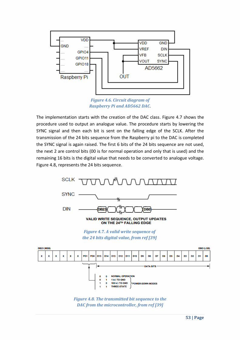
53 | Page
The implementation starts with the creation of the DAC class. Figure 4.7 shows the
procedure used to output an analogue value. The procedure starts by lowering the
SYNC signal and then each bit is sent on the falling edge of the SCLK. After the
transmission of the 24 bits sequence from the Raspberry pi to the DAC is completed
the SYNC signal is again raised. The first 6 bits of the 24 bits sequence are not used,
the next 2 are control bits (00 is for normal operation and only that is used) and the
remaining 16 bits is the digital value that needs to be converted to analogue voltage.
Figure 4.8, represents the 24 bits sequence.
Figure 4.6. Circuit diagram of
Raspberry Pi and AD5662 DAC.
Figure 4.7. A valid write sequence of
the 24 bits digital value, from ref [39]
Figure 4.8. The transmitted bit sequence to the
DAC from the microcontroller, from ref [39]
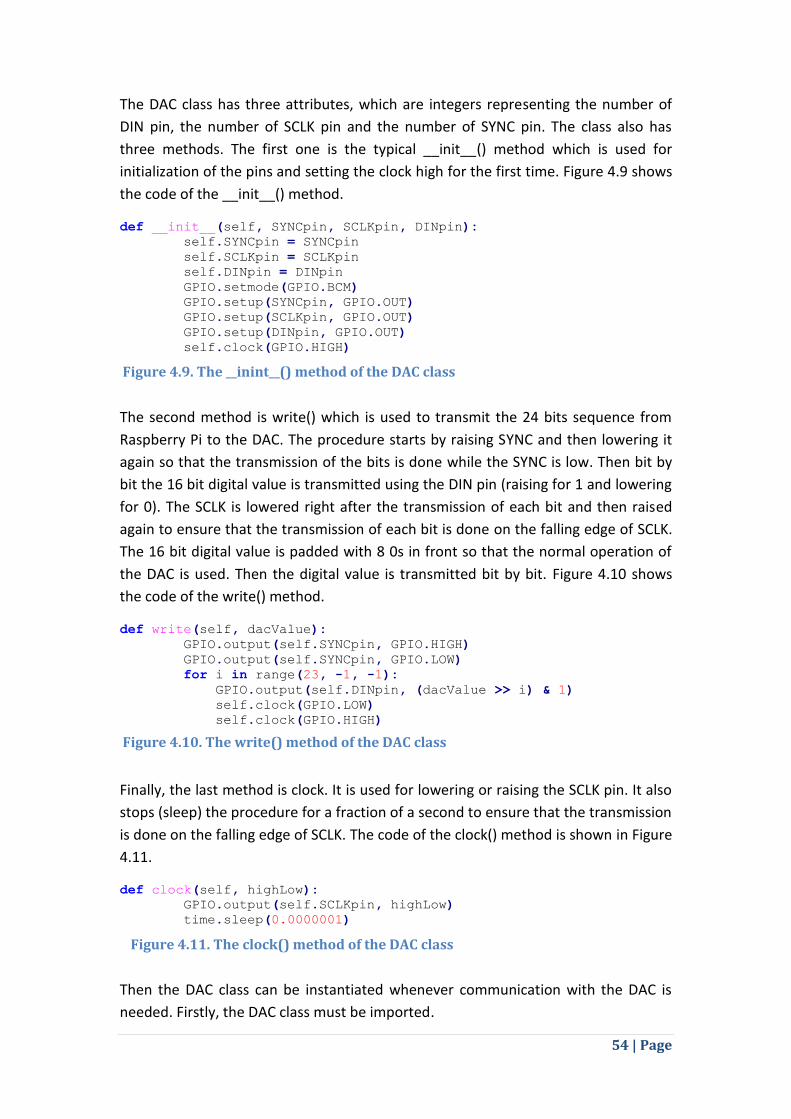
54 | Page
The DAC class has three attributes, which are integers representing the number of
DIN pin, the number of SCLK pin and the number of SYNC pin. The class also has
three methods. The first one is the typical __init__() method which is used for
initialization of the pins and setting the clock high for the first time. Figure 4.9 shows
the code of the __init__() method.
def __init__(self, SYNCpin, SCLKpin, DINpin): self.SYNCpin = SYNCpin self.SCLKpin = SCLKpin self.DINpin = DINpin GPIO.setmode(GPIO.BCM) GPIO.setup(SYNCpin, GPIO.OUT) GPIO.setup(SCLKpin, GPIO.OUT) GPIO.setup(DINpin, GPIO.OUT) self.clock(GPIO.HIGH)
The second method is write() which is used to transmit the 24 bits sequence from
Raspberry Pi to the DAC. The procedure starts by raising SYNC and then lowering it
again so that the transmission of the bits is done while the SYNC is low. Then bit by
bit the 16 bit digital value is transmitted using the DIN pin (raising for 1 and lowering
for 0). The SCLK is lowered right after the transmission of each bit and then raised
again to ensure that the transmission of each bit is done on the falling edge of SCLK.
The 16 bit digital value is padded with 8 0s in front so that the normal operation of
the DAC is used. Then the digital value is transmitted bit by bit. Figure 4.10 shows
the code of the write() method.
def write(self, dacValue):
GPIO.output(self.SYNCpin, GPIO.HIGH)
GPIO.output(self.SYNCpin, GPIO.LOW)
for i in range(23, -1, -1):
GPIO.output(self.DINpin, (dacValue >> i) & 1)
self.clock(GPIO.LOW)
self.clock(GPIO.HIGH)
Finally, the last method is clock. It is used for lowering or raising the SCLK pin. It also
stops (sleep) the procedure for a fraction of a second to ensure that the transmission
is done on the falling edge of SCLK. The code of the clock() method is shown in Figure
4.11.
def clock(self, highLow):
GPIO.output(self.SCLKpin, highLow)
time.sleep(0.0000001)
Then the DAC class can be instantiated whenever communication with the DAC is
needed. Firstly, the DAC class must be imported.
Figure 4.9. The __inint__() method of the DAC class
Figure 4.10. The write() method of the DAC class
Figure 4.11. The clock() method of the DAC class
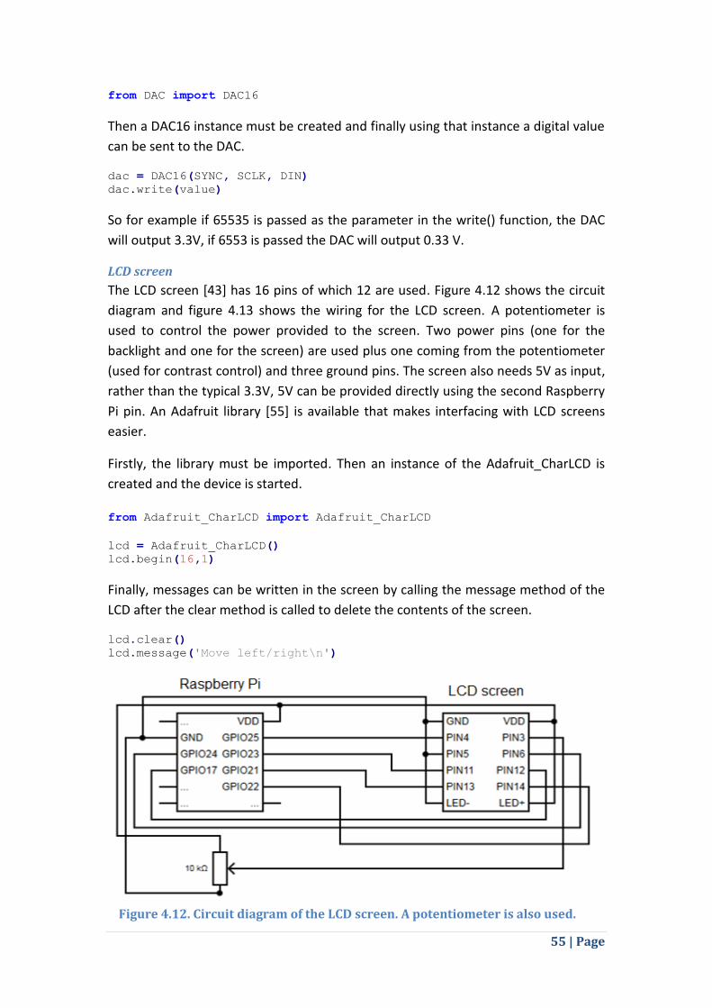
55 | Page
from DAC import DAC16
Then a DAC16 instance must be created and finally using that instance a digital value
can be sent to the DAC.
dac = DAC16(SYNC, SCLK, DIN) dac.write(value)
So for example if 65535 is passed as the parameter in the write() function, the DAC
will output 3.3V, if 6553 is passed the DAC will output 0.33 V.
LCD screen
The LCD screen [43] has 16 pins of which 12 are used. Figure 4.12 shows the circuit
diagram and figure 4.13 shows the wiring for the LCD screen. A potentiometer is
used to control the power provided to the screen. Two power pins (one for the
backlight and one for the screen) are used plus one coming from the potentiometer
(used for contrast control) and three ground pins. The screen also needs 5V as input,
rather than the typical 3.3V, 5V can be provided directly using the second Raspberry
Pi pin. An Adafruit library [55] is available that makes interfacing with LCD screens
easier.
Firstly, the library must be imported. Then an instance of the Adafruit_CharLCD is
created and the device is started.
from Adafruit_CharLCD import Adafruit_CharLCD
lcd = Adafruit_CharLCD()
lcd.begin(16,1)
Finally, messages can be written in the screen by calling the message method of the
LCD after the clear method is called to delete the contents of the screen.
lcd.clear()
lcd.message('Move left/right\n')
Figure 4.12. Circuit diagram of the LCD screen. A potentiometer is also used.

56 | Page
Heaters
Two 24 V, 6 mm diameter cartridge heaters are used for this system. The heaters are
attached in the two holes of the aluminium block. The two heaters are connected in
series and then they are connected to the external power supply output. Finally, the
external power supply volt input port (CV) is connected to the DAC output and the
common port of the TTi PL303 – P power supply [51] is connected to the ground.
The power supply is set to operate as a power amplifier of the DAC output in order
to produce enough power for the heaters. Figure 4.14 shows the circuit diagram
used for powering the heaters.
Figure 4.13. Physical wiring of the LCD screen with the Raspberry Pi.
Figure 4.14. Circuit diagram of the heaters and the external power supply.
DAC output is amplified by the power supply to power the heaters.

57 | Page
4.3 PID controller implementation
For both system identification methods, step response and parameter estimation,
there are four important steps that must be implemented:
Initial experiment, collect data required to model the system.
Modelling of the process, obtain transfer function model from the data of the
experiment using step response or parameter estimation.
PID controller tuning, obtain Kp, Ki, Kd (the model of the process is required
for this step).
Controller loop, continually generate the process input (e.g. power to the
heater) depending on the process output (e.g. temperature).
4.3.1 Initial experiment
First of all, data must be collected by running an experiment. Although, the
experiment must be performed for both step response and parameter estimation,
the procedure followed is different for the two methods. In the case of the step
response, a step in the value of controller output/process input is applied (step input
experiment). The duration of the experiment depends on the time needed for the
system to reach a new steady state. During the experiment both inputs and outputs
of the process are logged. In the case of parameter estimation, controller
output/process input is produced using a Pseudorandom Binary Signal (PRBS)
generator. The duration of the experiment is selected depending on the process (a
typical value is 30 seconds). Again during the experiment both inputs and outputs of
the process are logged. Also, steady state (heater off) input and output are also
logged in order to produce the deviation variables.
In both cases, the first task to be done is to create instances of the temperature
sensor class and the DAC class. Code for the instantiation of the classes is shown in
figure 4.15. Following the creation of the instances, the experiment is run.
GPIO.setmode(GPIO.BCM)
SENSOR_INPUT = 7
CLK = 9
sht1x = SHT1x(SENSOR_INPUT, CLK, SHT1x.GPIO_BCM)
DIN = 18
SCLK = 11
SYNC = 4
dac = DAC16(SYNC, SCLK, DIN)
Figure 4.15. Instantiation of the DAC and SHT1x classes
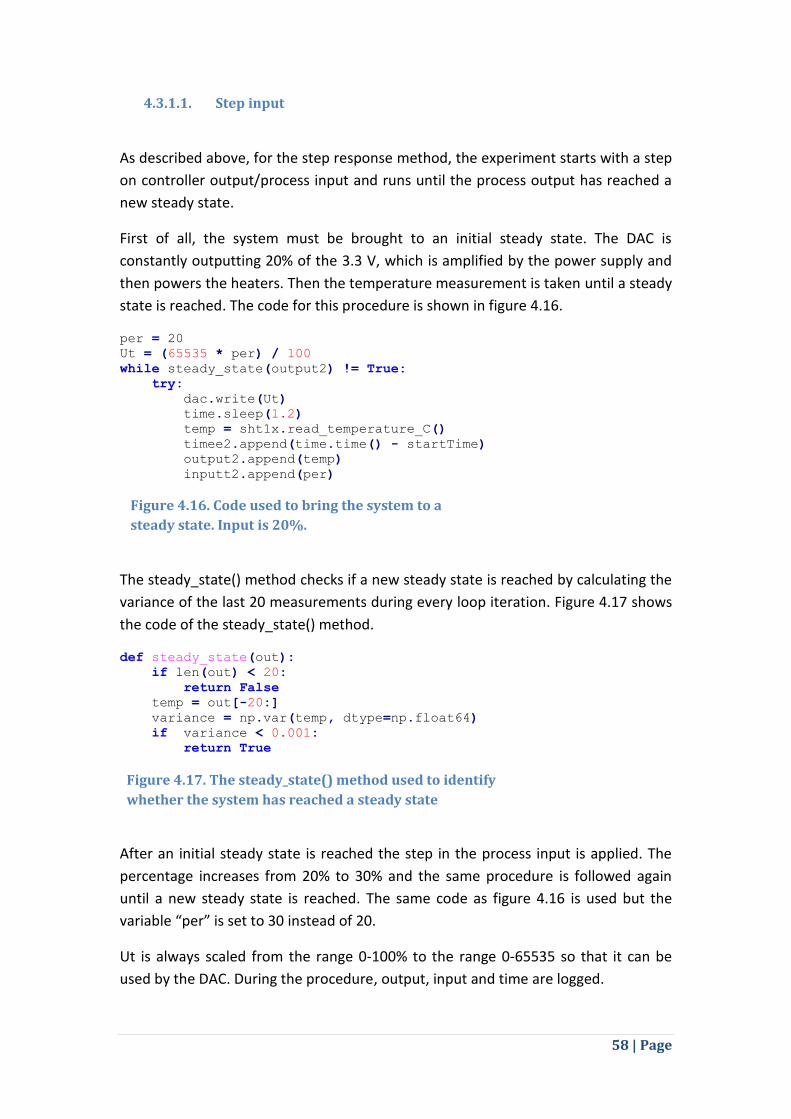
58 | Page
4.3.1.1. Step input
As described above, for the step response method, the experiment starts with a step
on controller output/process input and runs until the process output has reached a
new steady state.
First of all, the system must be brought to an initial steady state. The DAC is
constantly outputting 20% of the 3.3 V, which is amplified by the power supply and
then powers the heaters. Then the temperature measurement is taken until a steady
state is reached. The code for this procedure is shown in figure 4.16.
per = 20 Ut = (65535 * per) / 100 while steady_state(output2) != True: try: dac.write(Ut)
time.sleep(1.2) temp = sht1x.read_temperature_C() timee2.append(time.time() - startTime) output2.append(temp) inputt2.append(per)
The steady_state() method checks if a new steady state is reached by calculating the
variance of the last 20 measurements during every loop iteration. Figure 4.17 shows
the code of the steady_state() method.
def steady_state(out):
if len(out) < 20:
return False
temp = out[-20:]
variance = np.var(temp, dtype=np.float64)
if variance < 0.001:
return True
After an initial steady state is reached the step in the process input is applied. The
percentage increases from 20% to 30% and the same procedure is followed again
until a new steady state is reached. The same code as figure 4.16 is used but the
variable “per” is set to 30 instead of 20.
Ut is always scaled from the range 0-100% to the range 0-65535 so that it can be
used by the DAC. During the procedure, output, input and time are logged.
Figure 4.16. Code used to bring the system to a
steady state. Input is 20%.
Figure 4.17. The steady_state() method used to identify
whether the system has reached a steady state

59 | Page
4.3.1.2. PRBS
For parameter estimation, the experiment is different. The experiment starts by
setting the output value to one of the two possible values, e.g. 0 or 1, and selecting
the probability value p between 0 and 1. Then a value between 0 and 1 is randomly
produced and compared with probability p. If the random value produced is smaller
than probability p then the output value is switched to the other possible value. This
procedure is repeated a number of times, e.g. 30. The code used for the PRBS
experiment is shown in figure 4.18.
for i in range(30): dac.write(Ut) time.sleep(1.2) temp = sht1x.read_temperature_C() y.append(temp) u.append(power) timee.append(time.time() - startTime) k = random.random() if k < p: if Ut == 0: power = 100 else: power = 0 Ut = (power * 65535) / 100
As before, controller output Ut is scaled to the range of 0 to 65535 before passed on
the DAC to power the heaters. The output of the process is measured using the
temperature sensor and is logged. Input is logged as well. Furthermore, PRBS can be
used for both system identification and model accuracy evaluation.
Finally, for use with the parameter estimation method the output and input
variables must be transformed to error values. This is done simply by subtracting the
steady state output and input values from each output and input value logged from
the previous experiment (deviation from initial input and output). Steady state
values are gathered just before the PRBS experiment starts.
for i in range(1, len(y)):
output.append(y[i] - y0)
inputt.append(u[i] - u0)
Figure 4.18. Code used for the PRBS experiment.
Probability p used is 0.1 (10% chance).
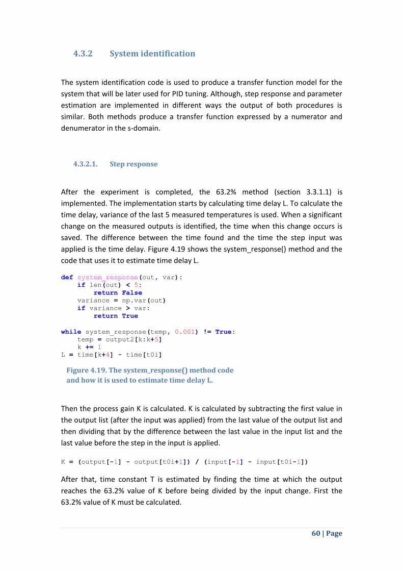
60 | Page
4.3.2 System identification
The system identification code is used to produce a transfer function model for the
system that will be later used for PID tuning. Although, step response and parameter
estimation are implemented in different ways the output of both procedures is
similar. Both methods produce a transfer function expressed by a numerator and
denumerator in the s-domain.
4.3.2.1. Step response
After the experiment is completed, the 63.2% method (section 3.3.1.1) is
implemented. The implementation starts by calculating time delay L. To calculate the
time delay, variance of the last 5 measured temperatures is used. When a significant
change on the measured outputs is identified, the time when this change occurs is
saved. The difference between the time found and the time the step input was
applied is the time delay. Figure 4.19 shows the system_response() method and the
code that uses it to estimate time delay L.
def system_response(out, var):
if len(out) < 5:
return False
variance = np.var(out)
if variance > var:
return True
while system_response(temp, 0.001) != True:
temp = output2[k:k+5]
k += 1
L = time[k+4] - time[t0i]
Then the process gain K is calculated. K is calculated by subtracting the first value in
the output list (after the input was applied) from the last value of the output list and
then dividing that by the difference between the last value in the input list and the
last value before the step in the input is applied.
K = (output[-1] - output[t0i+1]) / (input[-1] - input[t0i-1])
After that, time constant T is estimated by finding the time at which the output
reaches the 63.2% value of K before being divided by the input change. First the
63.2% value of K must be calculated.
Figure 4.19. The system_response() method code
and how it is used to estimate time delay L.

61 | Page
T63 = (output[-1] - output[t0i+1]) * 0.632
Then the value in the output list that is closer to the 63.2% value is found and the
index is saved. value_closer() method code is shown in figure 4.20.
j = value_closer(output, T63)
def value_closer(out, val): min_diff = 999 index = 0 for i in range(len(out)): diff = math.fabs(out[i]-val) if diff < min_diff: index = i min_diff = diff return index
Finally, using the index, the corresponding value in the time list is found, which
equals to the time constant.
T = time[j]
As all three, K, L, T are now calculated they are fitted to the transfer function model
to produce the transfer function of the process. K is used as the coefficient of s0 in
the numerator of the system and T and 1 are used as the coefficients of s1 and s0
respectively in the denumerator. L denotes the time delay of the system. The
transfer function produced is (equation 4.1):
(4.1)
4.3.2.2. Parameter estimation
After the PRBS experiment is completed the procedure for the calculation of θ starts.
The procedure starts by forming the φ matrix. Firstly, the first row of the φ matrix is
initialized using the first value in the output and input lists.
ph = [[y[0], 0, u[0], 1]]
Then, the rest of the φ matrix is created using the values from the output and input
values again. For each row the first value is the current output, the second value is
the previous output, the third value is the current input and the forth value is the
Figure 4.20. Code of the value_closer() method used
to estimate the time constant T.

62 | Page
previous input. Equation 4.2 better shows that. The code used to form the φ matrix
is shown in figure 4.21.
, , , (4.2)
for j in range(1,len(output)):
for i in range(2*n):
newPh[2*n-(i+1)] = ph[j-1][2*n-(i+2)]
newPh[0] = output[j-1]
newPh[n] = inputt[j-1]
l = copy.deepcopy(newPh)
ph.append(l)
After that, the calculation of θ is done using matrix operations. θ is calculated by
following the equation 4.3. The implementation of equation 4.3 is shown in figure
4.22.
Φ (4.3)
phT = np.matrix(ph).T
phI = np.matrix(np.dot(phT, ph)).I
th = np.dot(np.dot(phI, phT), np.array(output))
th = th.tolist()[0]
Using variable th (θ) the system discrete transfer function is produced in the z-
domain by fitting the four values of θ to the equation 4.4.
(4.4)
tfun = tf([float(th[2]), float(th[3])], [1, float(-th[0]), float(-
th[1])])
Finally, the discrete transfer function is transferred to the s-domain using the d2c
function from the yottalab library [44].
sys = d2c(tfun, method='zoh')
4.3.3 PID controller tuning
With the transfer function of the process calculated, the procedure can proceed to
the PID tuning. PID tuning is done in two different ways for step response and
parameter estimation.
Figure 4.21. Code used to form the φ matrix
Figure 4.22. Code used to calculate the θ vector.
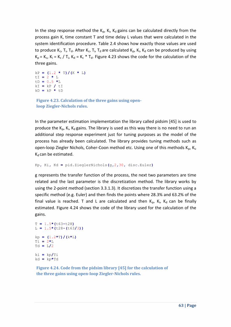
63 | Page
In the step response method the Kp, Ki, Kd gains can be calculated directly from the
process gain K, time constant T and time delay L values that were calculated in the
system identification procedure. Table 2.4 shows how exactly those values are used
to produce Kc, Ti, Td. After Kc, Ti, Td are calculated Kp, Ki, Kd can be produced by using
Kp = Kc, Ki = Kc / Ti, Kd = Kc * Td. Figure 4.23 shows the code for the calculation of the
three gains.
kP = (1.2 * T)/(K * L)
tI = 2 * L
tD = 0.5 *L
kI = kP / tI
kD = kP * tD
In the parameter estimation implementation the library called pidsim [45] is used to
produce the Kp, Ki, Kd gains. The library is used as this way there is no need to run an
additional step response experiment just for tuning purposes as the model of the
process has already been calculated. The library provides tuning methods such as
open-loop Ziegler Nichols, Coher-Coon method etc. Using one of this methods Kp, Ki,
Kd can be estimated.
Kp, Ki, Kd = pid.ZieglerNichols(g,2,30, disc.Euler)
g represents the transfer function of the process, the next two parameters are time
related and the last parameter is the discretization method. The library works by
using the 2-point method (section 3.3.1.3). It discretizes the transfer function using a
specific method (e.g. Euler) and then finds the points where 28.3% and 63.2% of the
final value is reached. T and L are calculated and then Kp, Ki, Kd can be finally
estimated. Figure 4.24 shows the code of the library used for the calculation of the
gains.
T = 1.5*(t63-t28)
L = 1.5*(t28-(t63/3))
kp = (1.2*T)/(k*L)
Ti = 2*L
Td = L/2
ki = kp/Ti
kd = kp*Td
Figure 4.23. Calculation of the three gains using open-
loop Ziegler-Nichols rules.
Figure 4.24. Code from the pidsim library [45] for the calculation of
the three gains using open-loop Ziegler-Nichols rules.

64 | Page
4.3.4 PID controller loop implementation
After Kp, Ki, Kd values are estimated the final PID controller implementation can be
completed. To implement the PID controller a separate PID class is used
(implementation modified from [46]). Firstly, a PID class instance is created using Kp,
Ki, Kd.
p = PID.PID(Kp, Ki, Kd)
The set point value is then provided, e.g. 25 degrees and an initial process output
measurement is taken. The PID controller is then updated with the latest
measurement and the controller outputs the value that is going to be used as the
process input. This procedure is constantly performed in a loop until it is stopped by
the user. The PID loop implementation is shown in figure 4.25.
SP = 25 p.setPoint(SP) startTime = time.time() while True: try: Ut = p.update(PV) u.append(int(Ut)) UtVolt = (65535 * Ut) / 100 dac.write(int(Ut))
time.sleep(2) PV = sht1x.read_temperature_C() m.append(PV) t.append(time.time() - startTime) except KeyboardInterrupt: GPIO.cleanup break
During the loop the process input Ut is updated by the PID controller and passed to
the DAC. The process output PV is measured using the temperature sensor and is
then fed back to the PID controller in order to produce the new Ut. The controller
output/process input Ut is in the range of 0-100%, therefore Ut is scaled to the range
0-65535 before is passed to the DAC in order to power the heaters (through the
power supply). Finally, during the loop, input, output and time are logged using three
lists.
The PID controller uses the update method to receive the new PV value and produce
the new Ut value. The update method contains the main digital implementation of
the PID controller. First of all, the error is calculated by subtracting the current PV
value from the set point value.
self.error = self.set_point - current_value
Figure 4.25. Implementation of the PID controller loop.
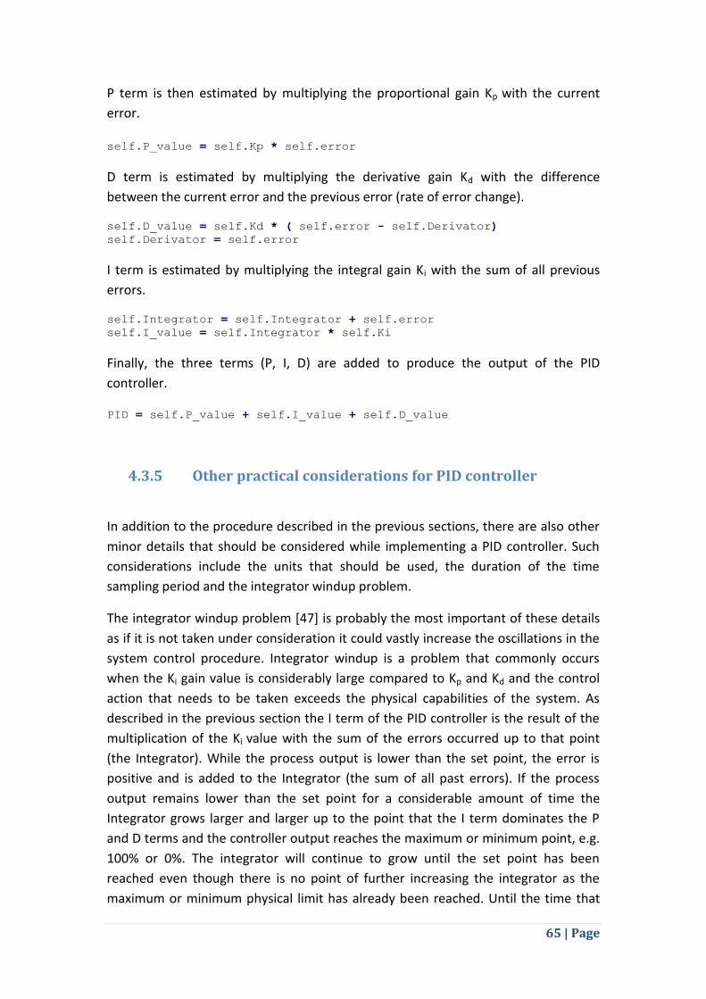
65 | Page
P term is then estimated by multiplying the proportional gain Kp with the current
error.
self.P_value = self.Kp * self.error
D term is estimated by multiplying the derivative gain Kd with the difference
between the current error and the previous error (rate of error change).
self.D_value = self.Kd * ( self.error - self.Derivator)
self.Derivator = self.error
I term is estimated by multiplying the integral gain Ki with the sum of all previous
errors.
self.Integrator = self.Integrator + self.error
self.I_value = self.Integrator * self.Ki
Finally, the three terms (P, I, D) are added to produce the output of the PID
controller.
PID = self.P_value + self.I_value + self.D_value
4.3.5 Other practical considerations for PID controller
In addition to the procedure described in the previous sections, there are also other
minor details that should be considered while implementing a PID controller. Such
considerations include the units that should be used, the duration of the time
sampling period and the integrator windup problem.
The integrator windup problem [47] is probably the most important of these details
as if it is not taken under consideration it could vastly increase the oscillations in the
system control procedure. Integrator windup is a problem that commonly occurs
when the Ki gain value is considerably large compared to Kp and Kd and the control
action that needs to be taken exceeds the physical capabilities of the system. As
described in the previous section the I term of the PID controller is the result of the
multiplication of the Ki value with the sum of the errors occurred up to that point
(the Integrator). While the process output is lower than the set point, the error is
positive and is added to the Integrator (the sum of all past errors). If the process
output remains lower than the set point for a considerable amount of time the
Integrator grows larger and larger up to the point that the I term dominates the P
and D terms and the controller output reaches the maximum or minimum point, e.g.
100% or 0%. The integrator will continue to grow until the set point has been
reached even though there is no point of further increasing the integrator as the
maximum or minimum physical limit has already been reached. Until the time that
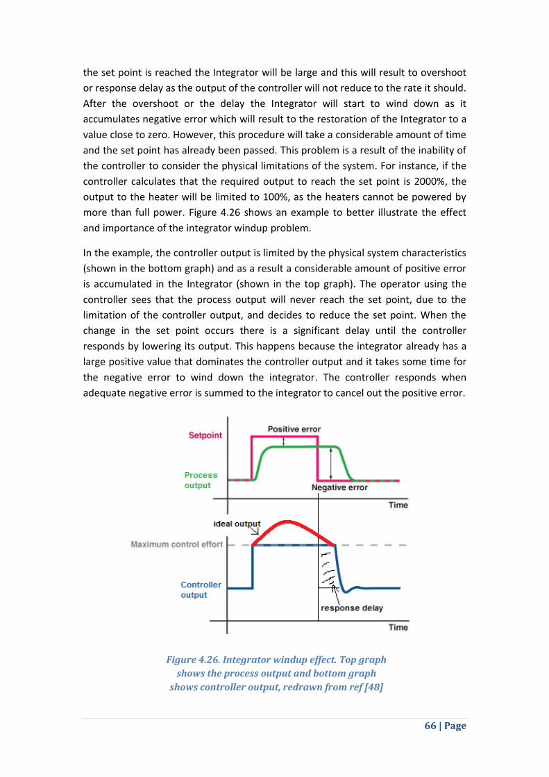
66 | Page
the set point is reached the Integrator will be large and this will result to overshoot
or response delay as the output of the controller will not reduce to the rate it should.
After the overshoot or the delay the Integrator will start to wind down as it
accumulates negative error which will result to the restoration of the Integrator to a
value close to zero. However, this procedure will take a considerable amount of time
and the set point has already been passed. This problem is a result of the inability of
the controller to consider the physical limitations of the system. For instance, if the
controller calculates that the required output to reach the set point is 2000%, the
output to the heater will be limited to 100%, as the heaters cannot be powered by
more than full power. Figure 4.26 shows an example to better illustrate the effect
and importance of the integrator windup problem.
In the example, the controller output is limited by the physical system characteristics
(shown in the bottom graph) and as a result a considerable amount of positive error
is accumulated in the Integrator (shown in the top graph). The operator using the
controller sees that the process output will never reach the set point, due to the
limitation of the controller output, and decides to reduce the set point. When the
change in the set point occurs there is a significant delay until the controller
responds by lowering its output. This happens because the integrator already has a
large positive value that dominates the controller output and it takes some time for
the negative error to wind down the integrator. The controller responds when
adequate negative error is summed to the integrator to cancel out the positive error.
Figure 4.26. Integrator windup effect. Top graph
shows the process output and bottom graph
shows controller output, redrawn from ref [48]

67 | Page
There are several solutions to solve this problem. In this case, clamping of the
controller output is used as the solution. Using this method, if the controller output
is larger or smaller than then physical limit, e.g. 100% or 0%, the controller output is
simply set to that limit. In addition, when the controller output is set to the
maximum or minimum limit, the integrator stops accumulating any more error. The
integrator restarts accumulating error when the value drops again between the
physical range or when the sign of the error is changed (the set point has been
passed). This way the response of the controller is faster when needed. Figure 4.27
shows the implementation of anti-windup method.
if PID > 100:
PID = 100
if self.set_point > current_value:
self.Integrator_flag = False
else:
self.Integrator_flag = True
elif PID < 0:
PID = 0
if self.set_point < current_value:
self.Integrator_flag = False
else:
self.Integrator_flag = True
else:
self.Integrator_flag = True
PID is the controller output value, which is clamped between 0 and 100.
Other considerations include the time period between the controller output and the
measurement of the process output (e.g. the temperature). This period is called the
sampling time or period of the system. The rule of thumb is that the sampling time
should be equal or smaller than the 1/10th of the time delay T [49]. So for example if
T is equal to 30 the sampling time should be 3 seconds or less. Generally, at least 10
measurements should be taken every T seconds.
Another minor but important issue is the units used for the controller input, the
controller output, the set point and the process output. The process output and the
set point should be expressed in the same units, as their difference will produce the
error value. For example, the process output and the set point can be in degrees
Celsius. To produce controller output that corresponds to the 0-100% range it is also
important that the process input used in the system identification experiments is
also in percentage and also in the same 0-100% range.
Figure 4.27. Implementation of the anti-windup method. Controller
output clamping is used and the error stops accumulating.
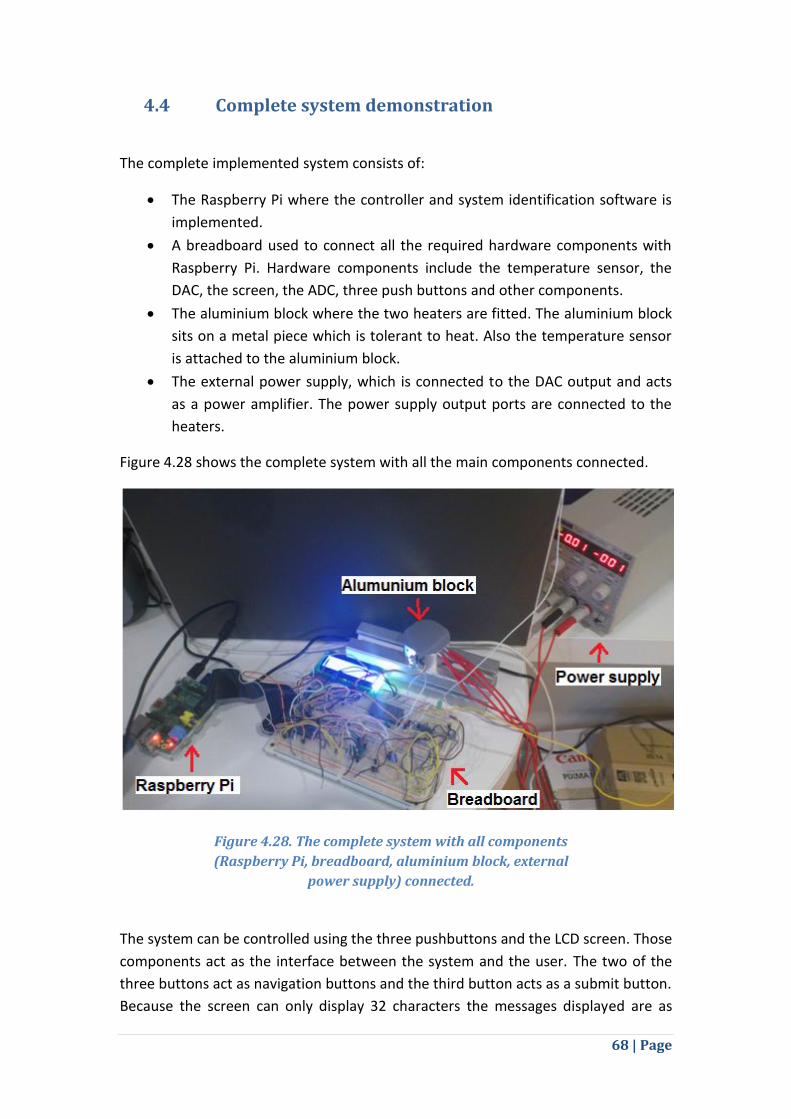
68 | Page
4.4 Complete system demonstration
The complete implemented system consists of:
The Raspberry Pi where the controller and system identification software is
implemented.
A breadboard used to connect all the required hardware components with
Raspberry Pi. Hardware components include the temperature sensor, the
DAC, the screen, the ADC, three push buttons and other components.
The aluminium block where the two heaters are fitted. The aluminium block
sits on a metal piece which is tolerant to heat. Also the temperature sensor
is attached to the aluminium block.
The external power supply, which is connected to the DAC output and acts
as a power amplifier. The power supply output ports are connected to the
heaters.
Figure 4.28 shows the complete system with all the main components connected.
The system can be controlled using the three pushbuttons and the LCD screen. Those
components act as the interface between the system and the user. The two of the
three buttons act as navigation buttons and the third button acts as a submit button.
Because the screen can only display 32 characters the messages displayed are as
Figure 4.28. The complete system with all components
(Raspberry Pi, breadboard, aluminium block, external
power supply) connected.
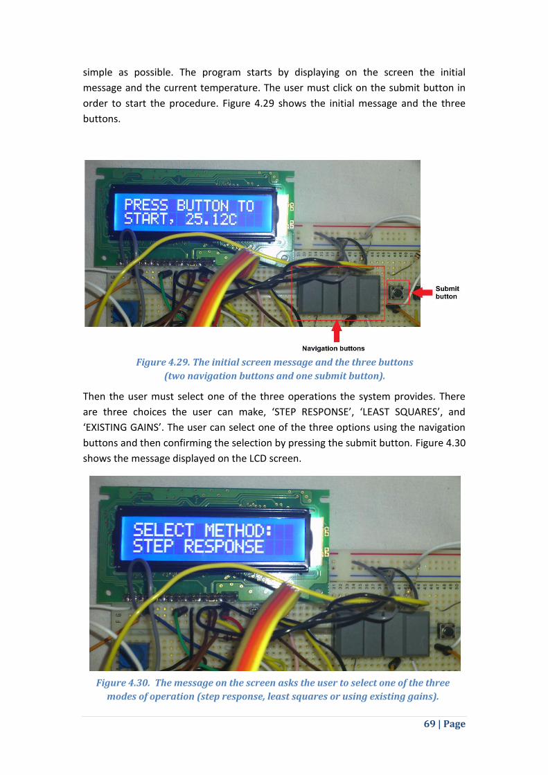
69 | Page
simple as possible. The program starts by displaying on the screen the initial
message and the current temperature. The user must click on the submit button in
order to start the procedure. Figure 4.29 shows the initial message and the three
buttons.
Then the user must select one of the three operations the system provides. There
are three choices the user can make, ‘STEP RESPONSE’, ‘LEAST SQUARES’, and
‘EXISTING GAINS’. The user can select one of the three options using the navigation
buttons and then confirming the selection by pressing the submit button. Figure 4.30
shows the message displayed on the LCD screen.
Figure 4.29. The initial screen message and the three buttons
(two navigation buttons and one submit button).
Figure 4.30. The message on the screen asks the user to select one of the three
modes of operation (step response, least squares or using existing gains).
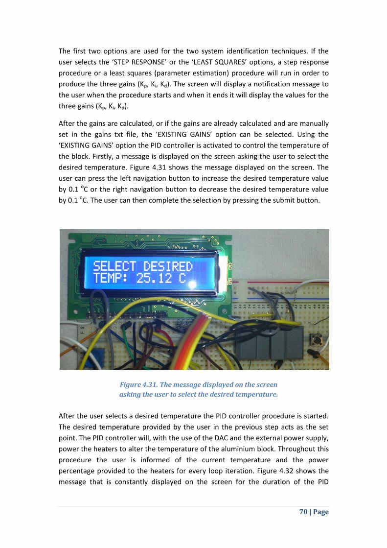
70 | Page
The first two options are used for the two system identification techniques. If the
user selects the ‘STEP RESPONSE’ or the ‘LEAST SQUARES’ options, a step response
procedure or a least squares (parameter estimation) procedure will run in order to
produce the three gains (Kp, Ki, Kd). The screen will display a notification message to
the user when the procedure starts and when it ends it will display the values for the
three gains (Kp, Ki, Kd).
After the gains are calculated, or if the gains are already calculated and are manually
set in the gains txt file, the ‘EXISTING GAINS’ option can be selected. Using the
‘EXISTING GAINS’ option the PID controller is activated to control the temperature of
the block. Firstly, a message is displayed on the screen asking the user to select the
desired temperature. Figure 4.31 shows the message displayed on the screen. The
user can press the left navigation button to increase the desired temperature value
by 0.1 oC or the right navigation button to decrease the desired temperature value
by 0.1 oC. The user can then complete the selection by pressing the submit button.
After the user selects a desired temperature the PID controller procedure is started.
The desired temperature provided by the user in the previous step acts as the set
point. The PID controller will, with the use of the DAC and the external power supply,
power the heaters to alter the temperature of the aluminium block. Throughout this
procedure the user is informed of the current temperature and the power
percentage provided to the heaters for every loop iteration. Figure 4.32 shows the
message that is constantly displayed on the screen for the duration of the PID
Figure 4.31. The message displayed on the screen
asking the user to select the desired temperature.
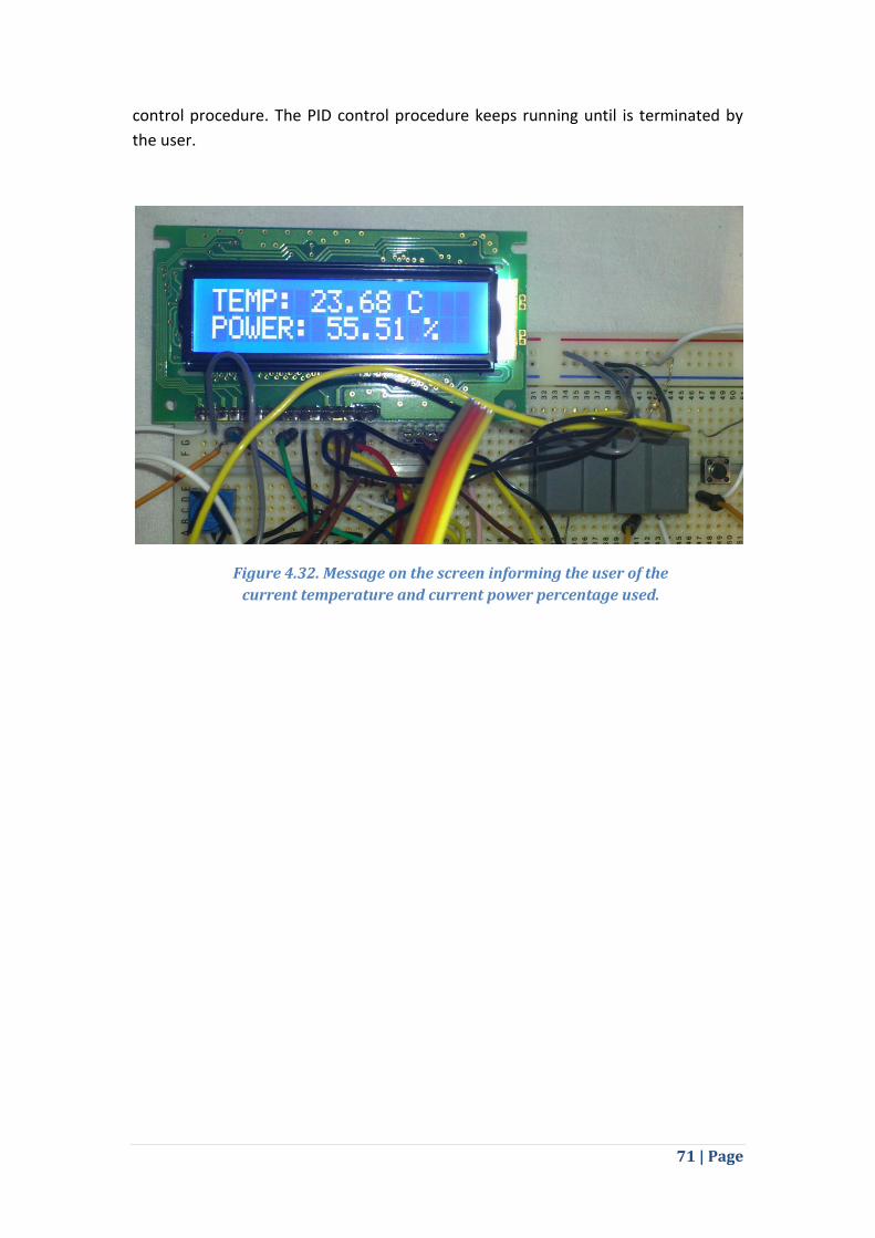
71 | Page
control procedure. The PID control procedure keeps running until is terminated by
the user.
Figure 4.32. Message on the screen informing the user of the
current temperature and current power percentage used.
72 | Page
5. Evaluation, Testing and Results
This chapter contains details about the evaluation procedure for all parts of the
system and the results produced after the evaluation.
The first section contains details about the measurement tools used and their
capabilities.
The second section describes how the hardware components were evaluated to
identify their actual resolution.
The third section describes the evaluation procedure for the two system
identification techniques, step response and parameter estimation. This sections
contains examples of the experiments used to evaluate these techniques and an
evaluation of the produced model accuracy compared to the real system. It also
shows how the PID gains are produced.
The forth section describes the evaluation of the PID controller. This section contains
examples of the control experiments. The PID controller is evaluated based on
several characteristics that a good control system should have. Furthermore, the
effectiveness of the controller using the gains produced by the two system
identification techniques is compared.
The fifth and last section summarizes the results of the evaluation and assesses the
success of the project.
5.1 Measurement tools
For proper evaluation and testing in this project, specialized equipment needs to be
used. Equipment includes external power supplies and accurate voltmeters. For the
evaluation of this project, two external devices were used, Keithley 2400
SourceMeter [50] and TTi PL303 – P power supply [51]. The Keithley 2400
SourceMeter is used during the evaluation of the ADC and DAC components.
Keithley 2400 can be used both as a voltage supply and as a voltage meter. It can
output and measure voltage in the range of -20 V to 20 V and current in the range of
-1 A to 1 A with a resolution 1-100 μV and 10 pA – 10 μA respectively (exact
resolution depends on the mode). TTi PL303 – P was used to amplify the DAC output
and as a current source, it can output up to 3A at 30V. One important feature of this

73 | Page
power supply and the main reason that it was used is voltage output amplification. It
can amplify a voltage input from the range of 0-5V to a range of 0-30V. In this
project, this feature was used to amplify the DAC output. This power supply was
used during the step input and PRBS experiments, the evaluation of the model of the
process and the evaluation of the PID controller.
5.2 Hardware components evaluation and testing
To be sure that the resolution of input and output is 16 bits both the ADC input and
DAC output need to be evaluated. Furthermore, the communication between the
Raspberry Pi and these components should be tested.
To evaluate and test the ADC a high accuracy calibrated (factory certified) voltage
supply (Keithley 2400) was used as an input to the ADC. The evaluation strategy was
as follows. The voltage readings provided by the ADC were compared with the
supplied voltage by the accurate voltage supply. The two values should be identical.
The voltage was kept stable for a period of time and then small changes in the
supplied voltage were provided. The new readings produced by the ADC were
checked to make sure they reflected those voltage changes.
To measure the resolution, the size of the step in the voltage supply is required. The
size of the step is determined by the voltage values range, which in this case is 0 V -
3.3 V and the range of distinct digital values that a given resolution provides. The
resolution tested first was 15 bits that results to a step of 0.1 mV or 0.0001 V (3300 /
215 ~= 0.0001). The evaluation procedure started by setting the accurate voltage
supply to 1000 mV, which provided 999.997 mV as displayed on the screen of the
Keithley. The measurement provided by the ADC was 999.562 mV, which is
considered accurate as the difference between this value and the provided value is
smaller than 0.5 mV. Then to test the resolution the input voltage was set, through
the Keithley, to 1000.1 mV a step of 0.1 mV from the previous setting. The measured
value provided by the ADC was 999.750 mV. The difference between the two
measurements was 0.188 mV. A third measurement was also taken with a 1000.2
mV setting. The ADC measurement was 999.938 mV. The difference with the
previous measurement was again 0.188 mV. Figure 5.1 shows graphically the
readings produced by the ADC over a period of 3 seconds, with a different voltage
input setting for each second. Using the difference between each step the practical
resolution can be calculated. The resolution for this ADC can be calculated by solving
0.188 * X = 3300. The solution is 17553 which is a value between 214 and 215. Thus
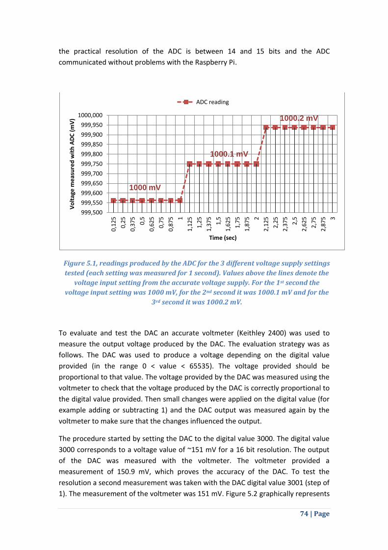
74 | Page
the practical resolution of the ADC is between 14 and 15 bits and the ADC
communicated without problems with the Raspberry Pi.
To evaluate and test the DAC an accurate voltmeter (Keithley 2400) was used to
measure the output voltage produced by the DAC. The evaluation strategy was as
follows. The DAC was used to produce a voltage depending on the digital value
provided (in the range 0 < value < 65535). The voltage provided should be
proportional to that value. The voltage provided by the DAC was measured using the
voltmeter to check that the voltage produced by the DAC is correctly proportional to
the digital value provided. Then small changes were applied on the digital value (for
example adding or subtracting 1) and the DAC output was measured again by the
voltmeter to make sure that the changes influenced the output.
The procedure started by setting the DAC to the digital value 3000. The digital value
3000 corresponds to a voltage value of ~151 mV for a 16 bit resolution. The output
of the DAC was measured with the voltmeter. The voltmeter provided a
measurement of 150.9 mV, which proves the accuracy of the DAC. To test the
resolution a second measurement was taken with the DAC digital value 3001 (step of
1). The measurement of the voltmeter was 151 mV. Figure 5.2 graphically represents
1000 mV
1000.1 mV
1000.2 mV
999,500
999,550
999,600
999,650
999,700
999,750
999,800
999,850
999,900
999,950
1000,000 0
,12
5
0,2
5
0,3
75
0,5
0,6
25
0,7
5
0,8
75
1
1,1
25
1,2
5
1,3
75
1,5
1,6
25
1,7
5
1,8
75
2
2,1
25
2,2
5
2,3
75
2,5
2,6
25
2,7
5
2,8
75
3
Vo
ltag
e m
eas
ure
d w
ith
AD
C (
mV
)
Time (sec)
ADC reading
Figure 5.1, readings produced by the ADC for the 3 different voltage supply settings
tested (each setting was measured for 1 second). Values above the lines denote the
voltage input setting from the accurate voltage supply. For the 1st second the
voltage input setting was 1000 mV, for the 2nd second it was 1000.1 mV and for the
3rd second it was 1000.2 mV.

75 | Page
the output of the DAC measured by the voltmeter. The difference between the two
measurements was 0.1 mV. Again solving the 0.1 * X = 3300 equation it gives 33000,
which is a value close to 215. Thus the actual resolution of the DAC is 15 bits and the
DAC communicated as expected with the Raspberry Pi.
5.3 System model evaluation
To extract the model of the system several experiments were performed. The
procedure of system identification was executed as described in sections 4.3.1 and
4.3.2. Both of the system identification techniques were used (Step response and
parameter estimation) and both were evaluated to determine which one produced
the best model transfer function. The evaluation system used for both techniques is
the one described in section 4.1 with the temperature sensor positioned in the side
of the aluminium block closer to the heaters. The procedure was similar for both of
those techniques. First an experiment was run, using a step input for step response
and PRBS for parameter estimation. Then using the step response or parameter
estimation identification method a system model was acquired. Based on that model
the three PID controller gains were estimated. Finally, after the procedure was
completed and a model was acquired the evaluation procedure started. To evaluate
whether the model offers an accurate representation of the actual system
simulations were run using MATLAB. The evaluation started by generating an input
(a step or a PRBS) and, using that input and the model, a simulation (in MATLAB) was
run. The simulation produced the output (temperature in deviation variables) based
150,7
150,8
150,9
151
151,1
151,2
151,3
3000 3000 3000 3000 3000 3000 3001 3001 3001 3001 3001 3001
Vo
ltag
e (
mV
)
Digital value
DAC voltage out
Figure 5.2, DAC voltage output in mV measured by the
voltmeter for 2 different digital values (3000 and 3001).

76 | Page
on the input and the system model that were provided. Then the same input was
used in the actual physical system. The output of the physical system was compared
to the output of the simulation. The two outputs should be similar if the model is an
accurate representation of the system. Figure 5.3 graphically shows the evaluation
procedure. In this section, the term input is used to describe the process
input/controller output, which is the voltage provided to the heaters. The term
output is used to describe the process output, which is the measured temperature.
The experiments performed in this section are open-loop with no feedback involved.
By running these tests, it is also verified that the system identification
implementation is working appropriately.
5.3.1 Step response
Many step response experiments were done, an example follows. The experiment
started with the step input. The step input procedure started by first bringing the
system to a steady state (steady temperature). The input used for this experiment
was 20% of the DAC output, which after the amplifying of the external power supply
resulted in 3.96 V provided to the heaters. The temperature started from 29.2 oC and
reached a steady state at 29.5 oC. After a steady state was reached the step in the
input could be applied. The input was stepped from 20% to 30% which resulted in
5.94 V provided to the heaters. The experiment was kept running until a new steady
state was reached. The new steady state was reached at 35.15 oC after 660 seconds.
Figure 5.4 shows the output of the system to the step input. The output started from
the first steady state which was 29.5 oC until the new steady state was reached.
Figure 5.3. The evaluation procedure used to validate the
accuracy of the model compared to the physical system.
Same input is used and outputs are compared, from ref [36]
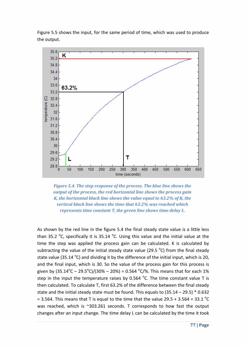
77 | Page
Figure 5.5 shows the input, for the same period of time, which was used to produce
the output.
As shown by the red line in the figure 5.4 the final steady state value is a little less
than 35.2 oC, specifically it is 35.14 oC. Using this value and the initial value at the
time the step was applied the process gain can be calculated. K is calculated by
subtracting the value of the initial steady state value (29.5 oC) from the final steady
state value (35.14 oC) and dividing it by the difference of the initial input, which is 20,
and the final input, which is 30. So the value of the process gain for this process is
given by (35.14oC – 29.5oC)/(30% – 20%) = 0.564 oC/%. This means that for each 1%
step in the input the temperature raises by 0.564 oC. The time constant value T is
then calculated. To calculate T, first 63.2% of the difference between the final steady
state and the initial steady state must be found. This equals to (35.14 – 29.5) * 0.632
= 3.564. This means that T is equal to the time that the value 29.5 + 3.564 = 33.1 oC
was reached, which is ~303.261 seconds. T corresponds to how fast the output
changes after an input change. The time delay L can be calculated by the time it took
Figure 5.4. The step response of the process. The blue line shows the
output of the process, the red horizontal line shows the process gain
K, the horizontal black line shows the value equal to 63.2% of K, the
vertical black line shows the time that 63.2% was reached which
represents time constant T, the green line shows time delay L.
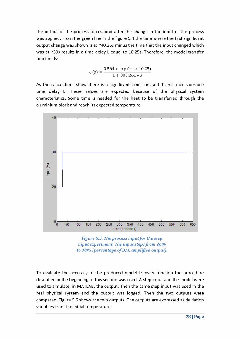
78 | Page
the output of the process to respond after the change in the input of the process
was applied. From the green line in the figure 5.4 the time where the first significant
output change was shown is at ~40.25s minus the time that the input changed which
was at ~30s results in a time delay L equal to 10.25s. Therefore, the model transfer
function is:
As the calculations show there is a significant time constant T and a considerable
time delay L. These values are expected because of the physical system
characteristics. Some time is needed for the heat to be transferred through the
aluminium block and reach its expected temperature.
To evaluate the accuracy of the produced model transfer function the procedure
described in the beginning of this section was used. A step input and the model were
used to simulate, in MATLAB, the output. Then the same step input was used in the
real physical system and the output was logged. Then the two outputs were
compared. Figure 5.6 shows the two outputs. The outputs are expressed as deviation
variables from the initial temperature.
Figure 5.5. The process input for the step
input experiment. The input steps from 20%
to 30% (percentage of DAC amplified output).

79 | Page
The comparisons show that the two outputs show some similarities and some
differences. The direction and shape of both output curves is similar, but there is a
difference in the final amplitude. This difference shows that the model produced
using the step response method overestimates the process gain compared to the
actual system. Other than the process gain, the time delay and time constant seem
to be accurate estimations.
Finally, the PID gains were calculated using the K, T and L values. The open-loop
Ziegler-Nichols tuning method rules were used for this procedure (table 2.4). Kc is
equal to (1.2 * 323.261)/(0.564 * 10.025) = 64.48, Ti is equal to 2 * 10.025 = 20,05
and Td is equal to 0.5 * 10.025 = 5.0125. Then Kp = Kc = 64.48, Ki = Kc / Ti = 3.21 and Kd
= Kc * Td = 323.26.
5.3.2 Parameter estimation
The same procedure was followed for the parameter estimation as well, with the
same evaluation system being used. The procedure for parameter estimation started
by generating a PRBS and using it as the input to the system. The procedure was
Figure 5.6. Comparison of the system actual output and the
simulation output using the same input. Output is expressed
as the amplitude of deviation from the initial temperature.

80 | Page
similar to the step response experiment. An input through the DAC was applied,
which was then scaled by the power supply and after a sampling period the output
(temperature) was measured and logged. Figure 5.7 shows the PRBS signal that was
used as the input of the system. The two possible values were 0% and 100%, which
correspond to 0V and 15.31V respectively. Figure 5.8 shows the output of the system
for this PRBS input.
Figure 5.7. The PRBS signal used as the input
for the parameter estimation experiment.
The possible values are 0% and 100%.
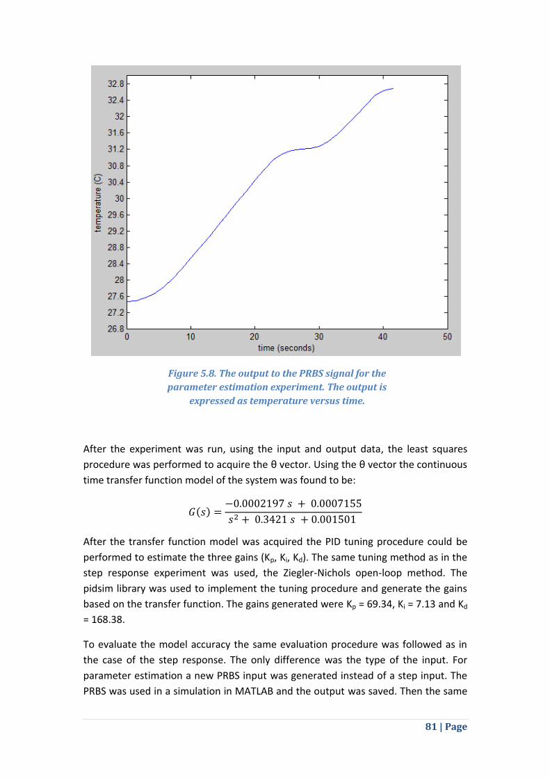
81 | Page
After the experiment was run, using the input and output data, the least squares
procedure was performed to acquire the θ vector. Using the θ vector the continuous
time transfer function model of the system was found to be:
After the transfer function model was acquired the PID tuning procedure could be
performed to estimate the three gains (Kp, Ki, Kd). The same tuning method as in the
step response experiment was used, the Ziegler-Nichols open-loop method. The
pidsim library was used to implement the tuning procedure and generate the gains
based on the transfer function. The gains generated were Kp = 69.34, Ki = 7.13 and Kd
= 168.38.
To evaluate the model accuracy the same evaluation procedure was followed as in
the case of the step response. The only difference was the type of the input. For
parameter estimation a new PRBS input was generated instead of a step input. The
PRBS was used in a simulation in MATLAB and the output was saved. Then the same
Figure 5.8. The output to the PRBS signal for the
parameter estimation experiment. The output is
expressed as temperature versus time.
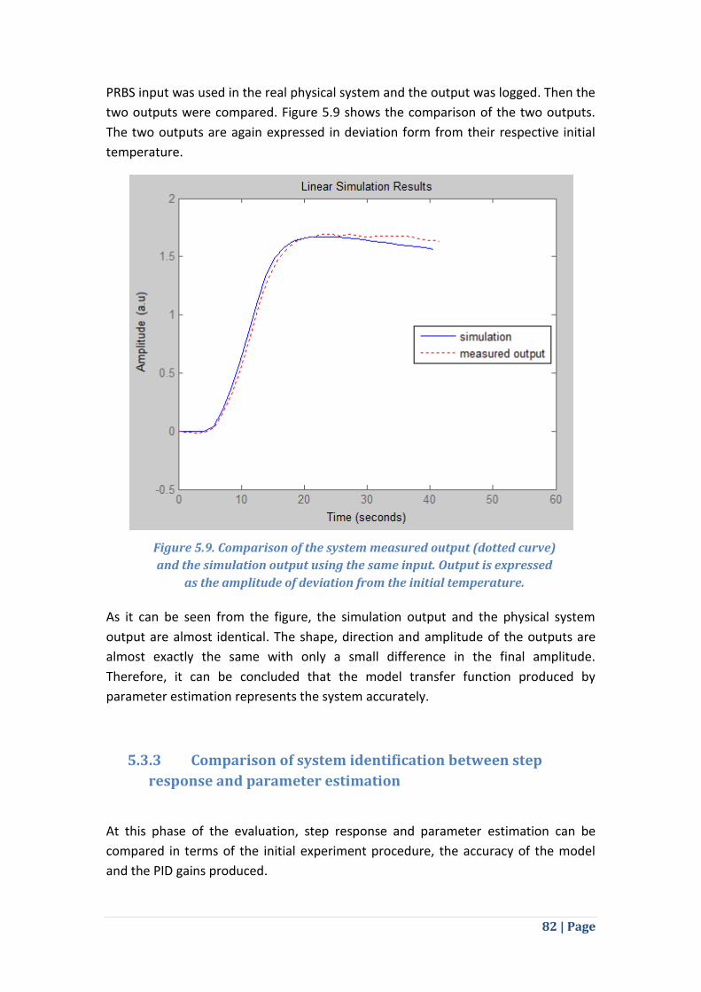
82 | Page
PRBS input was used in the real physical system and the output was logged. Then the
two outputs were compared. Figure 5.9 shows the comparison of the two outputs.
The two outputs are again expressed in deviation form from their respective initial
temperature.
As it can be seen from the figure, the simulation output and the physical system
output are almost identical. The shape, direction and amplitude of the outputs are
almost exactly the same with only a small difference in the final amplitude.
Therefore, it can be concluded that the model transfer function produced by
parameter estimation represents the system accurately.
5.3.3 Comparison of system identification between step
response and parameter estimation
At this phase of the evaluation, step response and parameter estimation can be
compared in terms of the initial experiment procedure, the accuracy of the model
and the PID gains produced.
Figure 5.9. Comparison of the system measured output (dotted curve)
and the simulation output using the same input. Output is expressed
as the amplitude of deviation from the initial temperature.
83 | Page
First of all, the implementation of both techniques worked as expected. All things
considered, parameter estimation appears to be the better option for system
identification. For the experiment procedure, the two methods require a different
process (step input and PRBS). In terms of the initial experiment procedure and the
accuracy of the produced model, parameter estimation provides a lot of advantages
compared to the step response method. Such advantages, compared to the step
response method, are:
Faster procedure, the experiment runs for a predefined period of time, which
can be less than 2 minutes. Step response experiments can run for a long
undefined period of time depending on the system (the time needed to reach
a new steady state).
The parameter estimation experiment does not have any prerequisites and
can be run no matter what state the system is in. Step response requires the
system to be brought to a steady state before the experiment starts, which
may require a considerable amount of time.
Can be used for every system without the need of any change. Step response
can also easily be used for every system but the definition of steady state
may be different in different systems (e.g. in this system 0.001 oC variance in
temperature, in a different system it could be 1 oC variance) and also the
amplitude in the step input may vary for different systems.
Produces a more accurate model. As shown during the evaluation of model
accuracy, parameter estimation produces a more accurate model.
However, the parameter estimation procedure also has some disadvantages
compared to step response, such as:
It is more complex to implement and understand. Step response system
identification procedure is straightforward and the model can be identified
directly from the plot.
The characteristics of the system extracted during the step response system
identification procedure give insight about the system. For example, the
amount of time required for the input change to take effect (time delay), etc.
Parameter estimation does not directly give any visible insight for the system.
Sometimes a PRBS experiment may need to be rerun. This may happen in the
case that the value in the PRBS signal is constantly the same, which although
is highly unlikely is possible.
In terms of the PID gains obtained by the two methods, Kp is around the same value
but Ki is more than double for parameter estimation and Kd is approximately half in
parameter estimation than the step response method. Based on the gains the
parameter estimation generated gains are expected to provide a faster response in
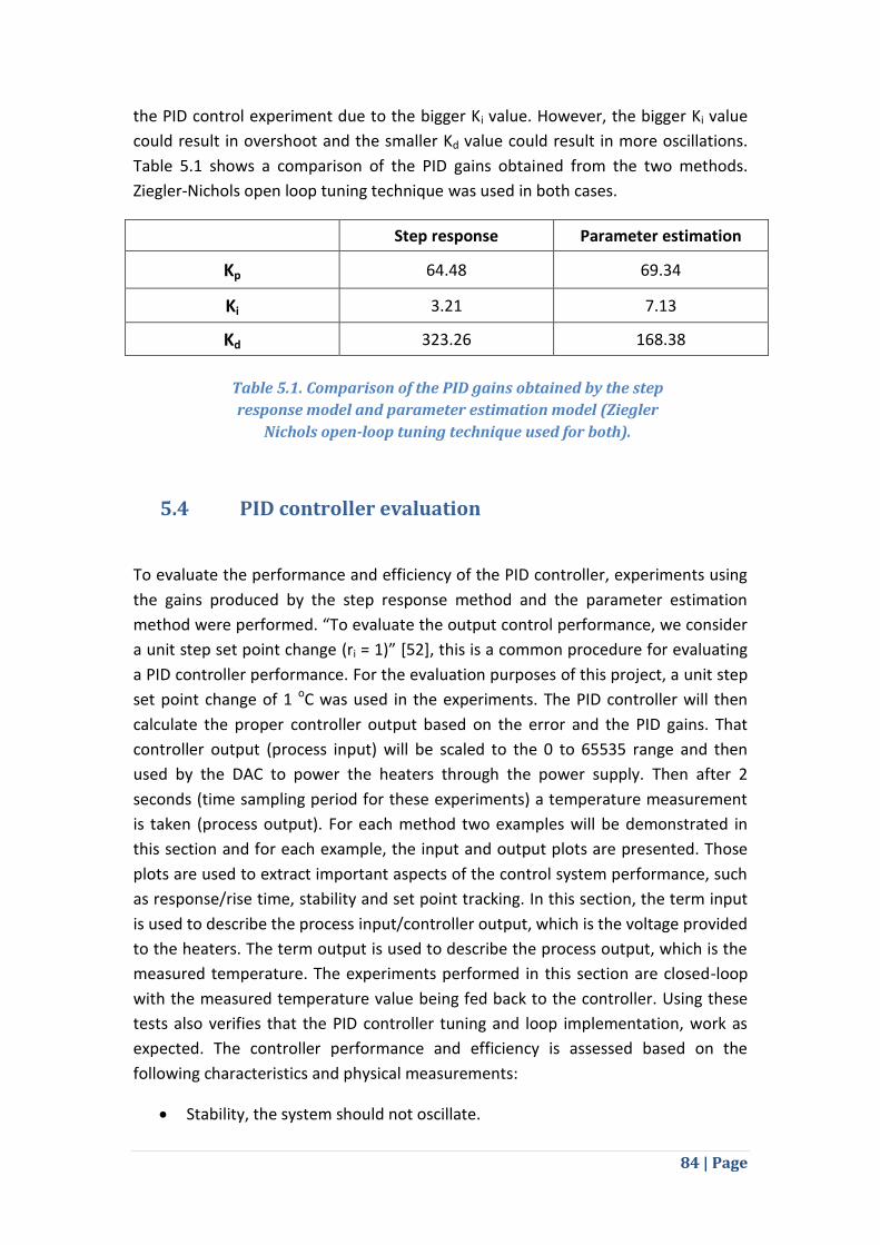
84 | Page
the PID control experiment due to the bigger Ki value. However, the bigger Ki value
could result in overshoot and the smaller Kd value could result in more oscillations.
Table 5.1 shows a comparison of the PID gains obtained from the two methods.
Ziegler-Nichols open loop tuning technique was used in both cases.
Step response Parameter estimation
Kp 64.48 69.34
Ki 3.21 7.13
Kd 323.26 168.38
5.4 PID controller evaluation
To evaluate the performance and efficiency of the PID controller, experiments using
the gains produced by the step response method and the parameter estimation
method were performed. “To evaluate the output control performance, we consider
a unit step set point change (ri = 1)” [52], this is a common procedure for evaluating
a PID controller performance. For the evaluation purposes of this project, a unit step
set point change of 1 oC was used in the experiments. The PID controller will then
calculate the proper controller output based on the error and the PID gains. That
controller output (process input) will be scaled to the 0 to 65535 range and then
used by the DAC to power the heaters through the power supply. Then after 2
seconds (time sampling period for these experiments) a temperature measurement
is taken (process output). For each method two examples will be demonstrated in
this section and for each example, the input and output plots are presented. Those
plots are used to extract important aspects of the control system performance, such
as response/rise time, stability and set point tracking. In this section, the term input
is used to describe the process input/controller output, which is the voltage provided
to the heaters. The term output is used to describe the process output, which is the
measured temperature. The experiments performed in this section are closed-loop
with the measured temperature value being fed back to the controller. Using these
tests also verifies that the PID controller tuning and loop implementation, work as
expected. The controller performance and efficiency is assessed based on the
following characteristics and physical measurements:
Stability, the system should not oscillate.
Table 5.1. Comparison of the PID gains obtained by the step
response model and parameter estimation model (Ziegler
Nichols open-loop tuning technique used for both).
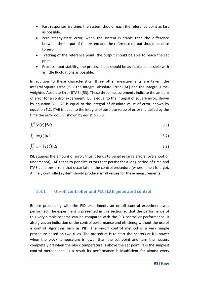
85 | Page
Fast response/rise time, the system should reach the reference point as fast
as possible.
Zero steady-state error, when the system is stable then the difference
between the output of the system and the reference output should be close
to zero.
Tracking of the reference point, the output should be able to reach the set
point.
Process input stability, the process input should be as stable as possible with
as little fluctuations as possible.
In addition to these characteristics, three other measurements are taken, the
Integral Square Error (ISE), the Integral Absolute Error (IAE) and the Integral Time-
weighted Absolute Error (ITAE) [53]. These three measurements indicate the amount
of error for a control experiment. ISE is equal to the integral of square error, shown
by equation 5.1. IAE is equal to the integral of absolute value of error, shown by
equation 5.2. ITAE is equal to the integral of absolute value of error multiplied by the
time the error occurs, shown by equation 5.3.
(5.1)
(5.2)
(5.3)
ISE squares the amount of error, thus it tends to penalize large errors (overshoot or
undershoot), IAE tends to penalize errors that persist for a long period of time and
ITAE penalizes errors that occur late in the control procedure (where time t is large).
A finely controlled system should produce small values for these measurements.
5.4.1 On-off controller and MATLAB generated control
Before proceeding with the PID experiments an on-off control experiment was
performed. The experiment is presented in this section so that the performance of
this very simple scheme can be compared with the PID controller performance. It
also gives an indication of the control performance and efficiency without the use of
a control algorithm such as PID. The on-off control method is a very simple
procedure based on two rules. The procedure is to start the heaters at full power
when the block temperature is lower than the set point and turn the heaters
completely off when the block temperature is above the set point. It is the simplest
control method and as a result its performance is insufficient for almost every
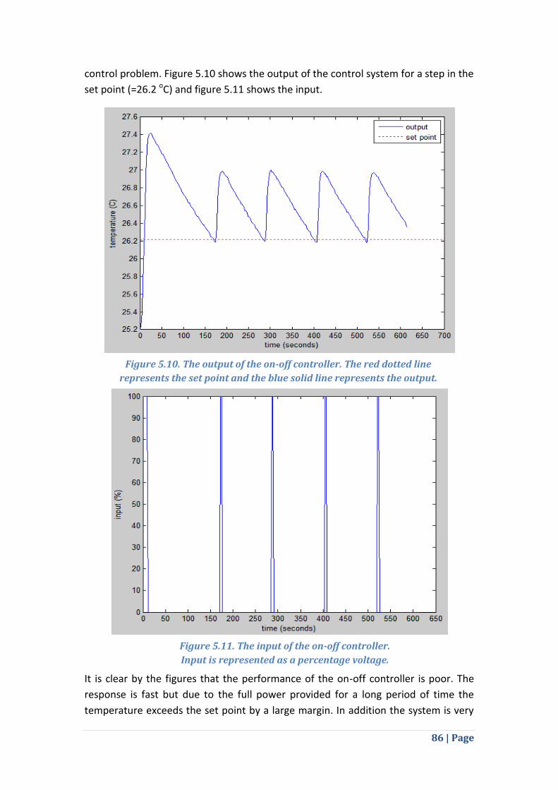
86 | Page
control problem. Figure 5.10 shows the output of the control system for a step in the
set point (=26.2 oC) and figure 5.11 shows the input.
It is clear by the figures that the performance of the on-off controller is poor. The
response is fast but due to the full power provided for a long period of time the
temperature exceeds the set point by a large margin. In addition the system is very
Figure 5.10. The output of the on-off controller. The red dotted line
represents the set point and the blue solid line represents the output.
Figure 5.11. The input of the on-off controller.
Input is represented as a percentage voltage.
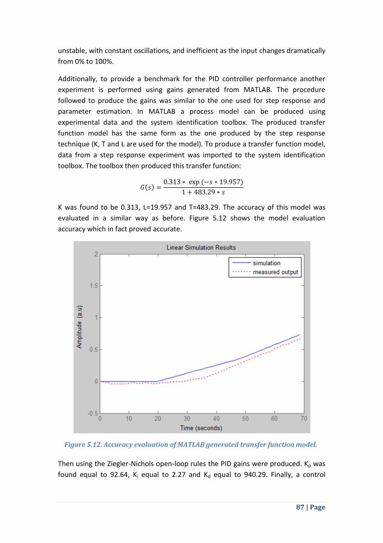
87 | Page
unstable, with constant oscillations, and inefficient as the input changes dramatically
from 0% to 100%.
Additionally, to provide a benchmark for the PID controller performance another
experiment is performed using gains generated from MATLAB. The procedure
followed to produce the gains was similar to the one used for step response and
parameter estimation. In MATLAB a process model can be produced using
experimental data and the system identification toolbox. The produced transfer
function model has the same form as the one produced by the step response
technique (K, T and L are used for the model). To produce a transfer function model,
data from a step response experiment was imported to the system identification
toolbox. The toolbox then produced this transfer function:
K was found to be 0.313, L=19.957 and T=483.29. The accuracy of this model was
evaluated in a similar way as before. Figure 5.12 shows the model evaluation
accuracy which in fact proved accurate.
Then using the Ziegler-Nichols open-loop rules the PID gains were produced. Kp was
found equal to 92.64, Ki equal to 2.27 and Kd equal to 940.29. Finally, a control
Figure 5.12. Accuracy evaluation of MATLAB generated transfer function model.
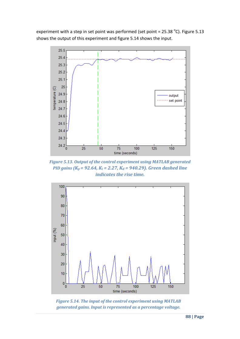
88 | Page
experiment with a step in set point was performed (set point = 25.38 oC). Figure 5.13
shows the output of this experiment and figure 5.14 shows the input.
Figure 5.13. Output of the control experiment using MATLAB generated
PID gains (Kp = 92.64, Ki = 2.27, Kd = 940.29). Green dashed line
indicates the rise time.
Figure 5.14. The input of the control experiment using MATLAB
generated gains. Input is represented as a percentage voltage.
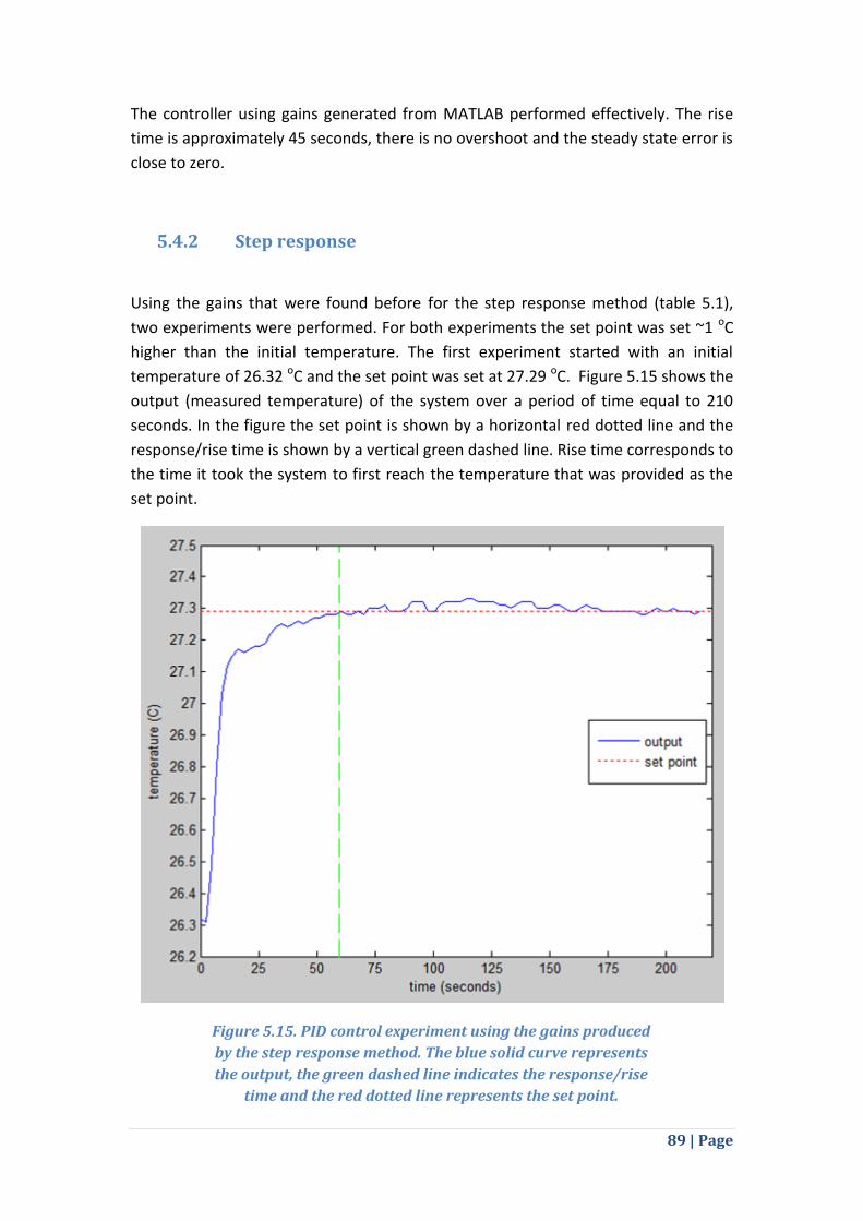
89 | Page
The controller using gains generated from MATLAB performed effectively. The rise
time is approximately 45 seconds, there is no overshoot and the steady state error is
close to zero.
5.4.2 Step response
Using the gains that were found before for the step response method (table 5.1),
two experiments were performed. For both experiments the set point was set ~1 oC
higher than the initial temperature. The first experiment started with an initial
temperature of 26.32 oC and the set point was set at 27.29 oC. Figure 5.15 shows the
output (measured temperature) of the system over a period of time equal to 210
seconds. In the figure the set point is shown by a horizontal red dotted line and the
response/rise time is shown by a vertical green dashed line. Rise time corresponds to
the time it took the system to first reach the temperature that was provided as the
set point.
Figure 5.15. PID control experiment using the gains produced
by the step response method. The blue solid curve represents
the output, the green dashed line indicates the response/rise
time and the red dotted line represents the set point.
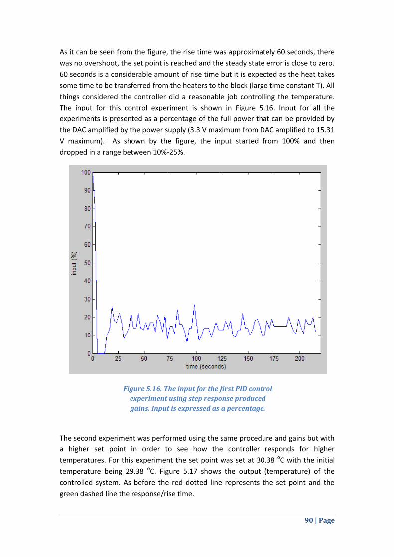
90 | Page
As it can be seen from the figure, the rise time was approximately 60 seconds, there
was no overshoot, the set point is reached and the steady state error is close to zero.
60 seconds is a considerable amount of rise time but it is expected as the heat takes
some time to be transferred from the heaters to the block (large time constant T). All
things considered the controller did a reasonable job controlling the temperature.
The input for this control experiment is shown in Figure 5.16. Input for all the
experiments is presented as a percentage of the full power that can be provided by
the DAC amplified by the power supply (3.3 V maximum from DAC amplified to 15.31
V maximum). As shown by the figure, the input started from 100% and then
dropped in a range between 10%-25%.
The second experiment was performed using the same procedure and gains but with
a higher set point in order to see how the controller responds for higher
temperatures. For this experiment the set point was set at 30.38 oC with the initial
temperature being 29.38 oC. Figure 5.17 shows the output (temperature) of the
controlled system. As before the red dotted line represents the set point and the
green dashed line the response/rise time.
Figure 5.16. The input for the first PID control
experiment using step response produced
gains. Input is expressed as a percentage.

91 | Page
The result of this experiment is similar to the result of the first one. Again there is no
overshoot or oscillations and the steady state error is close to zero. The only
difference is the rise time which is larger in this experiment, approximately 80
seconds, than the first one, approximately 60 seconds. This is probably due to the
higher temperature of the set point. It is harder for the block to heat in higher
temperatures. Apart from the rise time, which can be improved, the controller again
controlled the temperature successfully. Figure 5.18 shows the input for this
experiment, which as before is expressed in a percentage of power. For this
experiment the initial input is 100% as before and then it drops in the range of 15%-
30%, which is higher than the first experiment (10%-25%). This happens because of
the higher temperature as more power is required to provide more heat.
Figure 5.17. Second PID control experiment using the gains
produced by the step response method. The blue solid curve
represents the output, the green dashed line indicates the
response time and the red dotted line represents the set point.

92 | Page
5.4.3 Parameter estimation
The same procedure that was followed for step response was used for parameter
estimation. The PID gains used are those found during the parameter estimation
system identification procedure (Table 5.1). Two examples are again presented in
this section, one with a lower and one with a higher temperature. Furthermore, as
before, the set point was set ~1 oC higher than the initial temperature. The first
experiment started with an initial temperature of 27.18 oC and the set point was set
at 28.16 oC. The results of the control experiment are shown in figure 5.19. Output,
response/rise time and set point are presented in the plot the same way as in the
previous experiments. Figure 5.20 shows the corresponding input which is again
presented as a percentage of power.
Figure 5.18. The input for the second PID control
experiment using step response produced gains.
Input is expressed as a percentage.
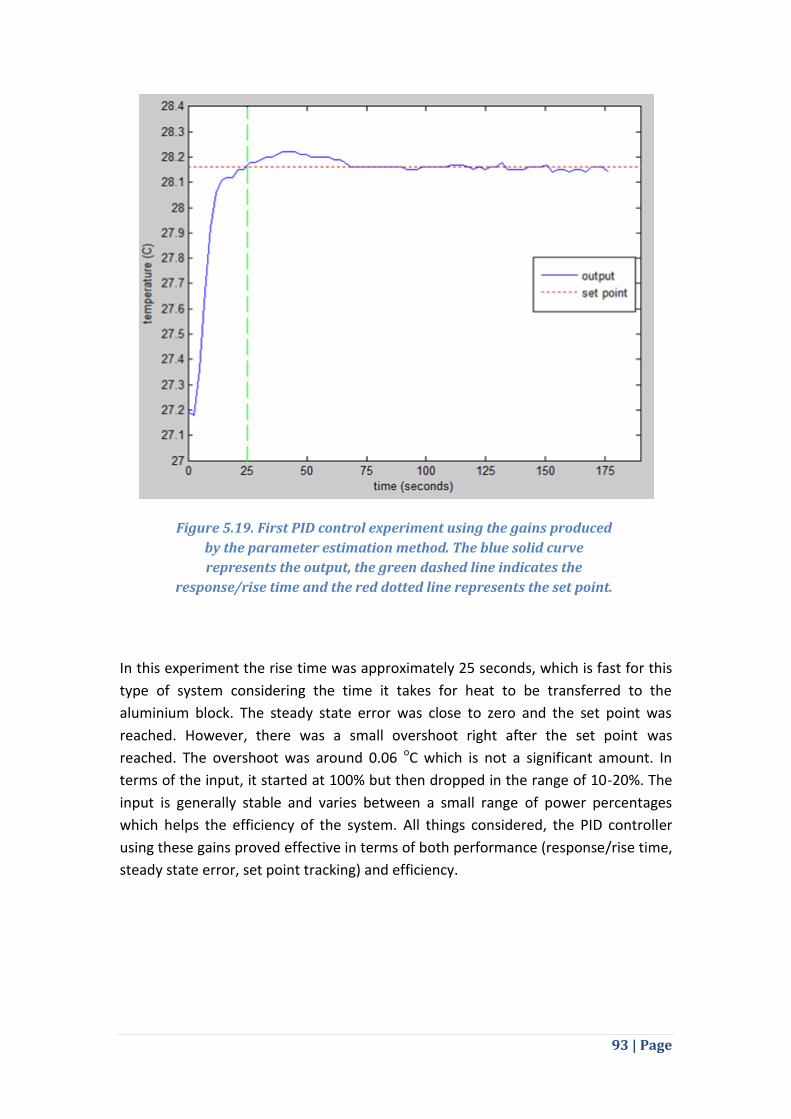
93 | Page
In this experiment the rise time was approximately 25 seconds, which is fast for this
type of system considering the time it takes for heat to be transferred to the
aluminium block. The steady state error was close to zero and the set point was
reached. However, there was a small overshoot right after the set point was
reached. The overshoot was around 0.06 oC which is not a significant amount. In
terms of the input, it started at 100% but then dropped in the range of 10-20%. The
input is generally stable and varies between a small range of power percentages
which helps the efficiency of the system. All things considered, the PID controller
using these gains proved effective in terms of both performance (response/rise time,
steady state error, set point tracking) and efficiency.
Figure 5.19. First PID control experiment using the gains produced
by the parameter estimation method. The blue solid curve
represents the output, the green dashed line indicates the
response/rise time and the red dotted line represents the set point.
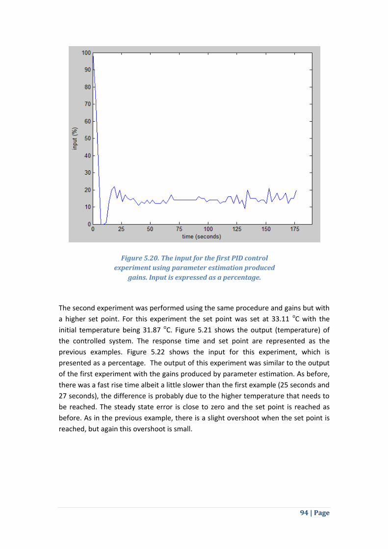
94 | Page
The second experiment was performed using the same procedure and gains but with
a higher set point. For this experiment the set point was set at 33.11 oC with the
initial temperature being 31.87 oC. Figure 5.21 shows the output (temperature) of
the controlled system. The response time and set point are represented as the
previous examples. Figure 5.22 shows the input for this experiment, which is
presented as a percentage. The output of this experiment was similar to the output
of the first experiment with the gains produced by parameter estimation. As before,
there was a fast rise time albeit a little slower than the first example (25 seconds and
27 seconds), the difference is probably due to the higher temperature that needs to
be reached. The steady state error is close to zero and the set point is reached as
before. As in the previous example, there is a slight overshoot when the set point is
reached, but again this overshoot is small.
Figure 5.20. The input for the first PID control
experiment using parameter estimation produced
gains. Input is expressed as a percentage.
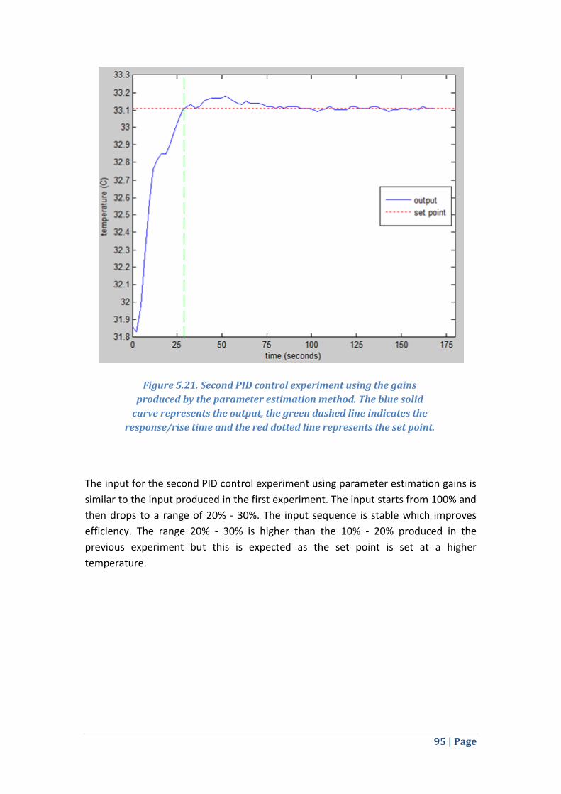
95 | Page
The input for the second PID control experiment using parameter estimation gains is
similar to the input produced in the first experiment. The input starts from 100% and
then drops to a range of 20% - 30%. The input sequence is stable which improves
efficiency. The range 20% - 30% is higher than the 10% - 20% produced in the
previous experiment but this is expected as the set point is set at a higher
temperature.
Figure 5.21. Second PID control experiment using the gains
produced by the parameter estimation method. The blue solid
curve represents the output, the green dashed line indicates the
response/rise time and the red dotted line represents the set point.
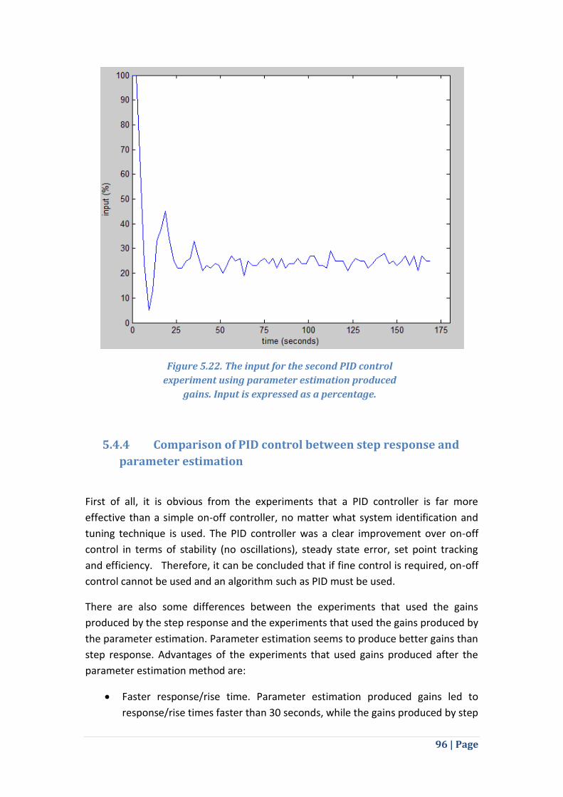
96 | Page
5.4.4 Comparison of PID control between step response and
parameter estimation
First of all, it is obvious from the experiments that a PID controller is far more
effective than a simple on-off controller, no matter what system identification and
tuning technique is used. The PID controller was a clear improvement over on-off
control in terms of stability (no oscillations), steady state error, set point tracking
and efficiency. Therefore, it can be concluded that if fine control is required, on-off
control cannot be used and an algorithm such as PID must be used.
There are also some differences between the experiments that used the gains
produced by the step response and the experiments that used the gains produced by
the parameter estimation. Parameter estimation seems to produce better gains than
step response. Advantages of the experiments that used gains produced after the
parameter estimation method are:
Faster response/rise time. Parameter estimation produced gains led to
response/rise times faster than 30 seconds, while the gains produced by step
Figure 5.22. The input for the second PID control
experiment using parameter estimation produced
gains. Input is expressed as a percentage.
97 | Page
response led to response/rise times slower than 60 seconds. A difference of
30 seconds is considerable.
More stable input. Using the gains produced by parameter estimation led to
an input in the range of 10% - 20% and 20% - 30% for the two experiments.
In contrast, the gains produced by step response led to an input in the range
of 10% - 25% and 15% - 30% for the two experiments. A smaller range results
in more efficiency.
On the other hand, the experiments using parameter estimation produced gains
have one disadvantage compared to the experiments using step response produced
gains:
There is a slight overshoot after the set point is reached in the parameter
estimation experiments. The step response experiments do not appear to
have such an overshoot.
The difference in response/rise time is probably an effect of the difference in the
integral gain (Ki). The parameter estimation method produces an integral gain equal
to 7.13 while the step response produces an integral gain equal to 3.21. The bigger
the integral gain the faster the response is. However, a bigger integral gain, along
with a smaller derivative gain (Kd is 168.38 for parameter estimation compared to
323.26 for step response), can also be the explanation for the slight overshoot
presented in the experiments using parameter estimation gains. Table 5.2 shows a
comparison between the four different techniques, on-off control, PID with gains
generated using MATLAB, PID with gains produced by the step response identified
model and PID with gains produced by the parameter estimation identified model.
The comparison uses data from the experiments presented in the previous sections
(for step response and parameter estimation data from the first of the two
experiments is used). For the ISE, IAE and ITAE measurements the experiments were
all reduced up to the 150th second in order for the measurements to be fair.
Between these four techniques parameter estimation gains seem to have the best
performance and efficiency, although it has a slight overshoot. MATLAB generated
gains also produce decent control, although the input range is large compared to the
other two methods. Furthermore, parameter estimation gains produced the best
measurements for IAE and ITAE and only 0.07 worse than MATLAB gains for ISE (ISE
tends to penalize overshoot). Step response gains also produced decent results,
although the rise time was larger than the other two techniques. This is the reason
why it produced worse values for IAE and ITAE than parameter estimation and
MATLAB gains. Finally, the inferiority of on-off control is obvious in all
measurements.
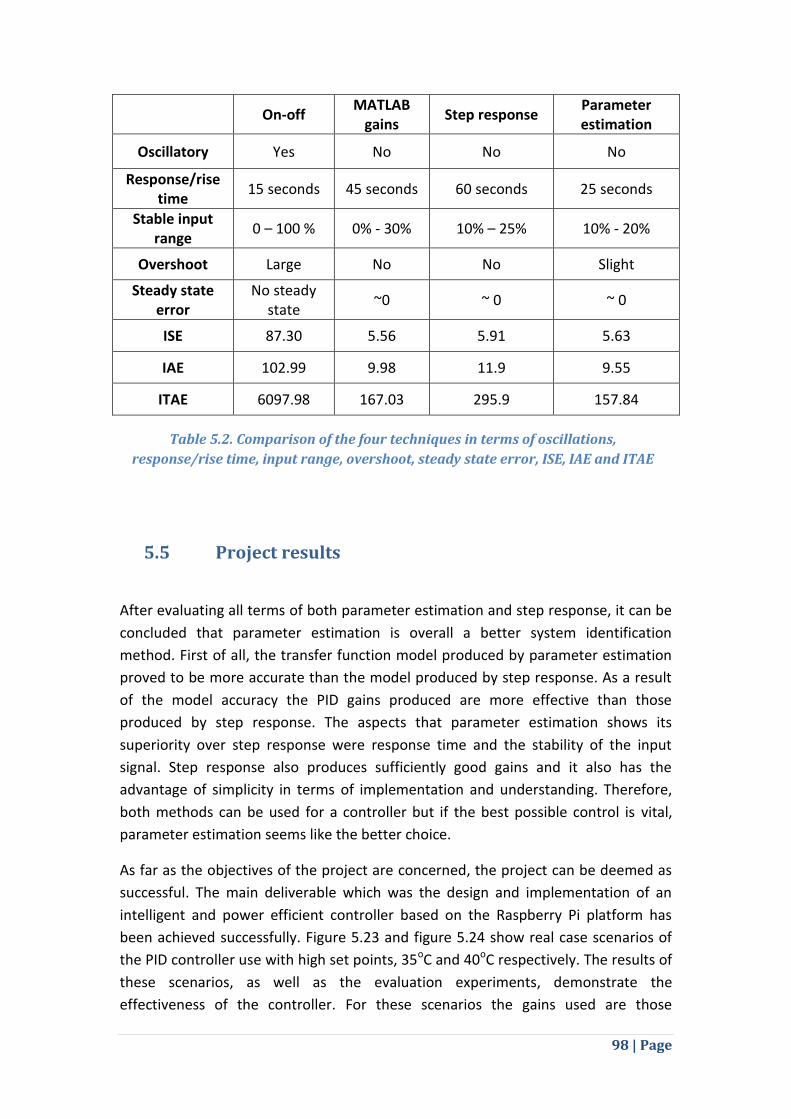
98 | Page
On-off MATLAB
gains Step response
Parameter estimation
Oscillatory Yes No No No
Response/rise time
15 seconds 45 seconds 60 seconds 25 seconds
Stable input range
0 – 100 % 0% - 30% 10% – 25% 10% - 20%
Overshoot Large No No Slight
Steady state error
No steady state
~0 ~ 0 ~ 0
ISE 87.30 5.56 5.91 5.63
IAE 102.99 9.98 11.9 9.55
ITAE 6097.98 167.03 295.9 157.84
5.5 Project results
After evaluating all terms of both parameter estimation and step response, it can be
concluded that parameter estimation is overall a better system identification
method. First of all, the transfer function model produced by parameter estimation
proved to be more accurate than the model produced by step response. As a result
of the model accuracy the PID gains produced are more effective than those
produced by step response. The aspects that parameter estimation shows its
superiority over step response were response time and the stability of the input
signal. Step response also produces sufficiently good gains and it also has the
advantage of simplicity in terms of implementation and understanding. Therefore,
both methods can be used for a controller but if the best possible control is vital,
parameter estimation seems like the better choice.
As far as the objectives of the project are concerned, the project can be deemed as
successful. The main deliverable which was the design and implementation of an
intelligent and power efficient controller based on the Raspberry Pi platform has
been achieved successfully. Figure 5.23 and figure 5.24 show real case scenarios of
the PID controller use with high set points, 35oC and 40oC respectively. The results of
these scenarios, as well as the evaluation experiments, demonstrate the
effectiveness of the controller. For these scenarios the gains used are those
Table 5.2. Comparison of the four techniques in terms of oscillations,
response/rise time, input range, overshoot, steady state error, ISE, IAE and ITAE
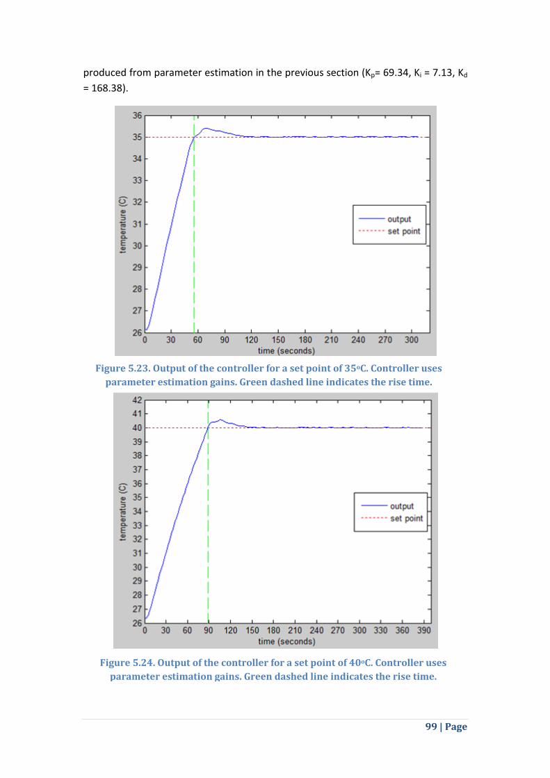
99 | Page
produced from parameter estimation in the previous section (Kp= 69.34, Ki = 7.13, Kd
= 168.38).
Figure 5.23. Output of the controller for a set point of 35oC. Controller uses
parameter estimation gains. Green dashed line indicates the rise time.
Figure 5.24. Output of the controller for a set point of 40oC. Controller uses
parameter estimation gains. Green dashed line indicates the rise time.
100 | Page
Similarly to the evaluation procedure, the controller is effective, offering stability
and fast response. There is a very small overshoot (lower than 0.4 oC) in both cases
but as seen in the evaluation procedure, it is a trade-off for the fast response time
and it does not affect the control of the system.
Furthermore, the additional deliverable of the project, which is the controller
produced to be sufficiently flexible in order to be able to control a variety of systems,
has also been achieved. Thanks to the empirical system identification techniques
used, a transfer function model can be produced for any system with no
modifications (parameter estimation) or few modifications (step response). Using
the transfer function model and an open-loop tuning technique, PID gains can be
estimated for every type of system automatically without the need of any manual
tuning. The last additional deliverable of integrating the system in a stand-alone
device was not implemented. That deliverable was prioritized last and it would have
been implemented only if sufficient time was left. Furthermore, the addition of an
external power supply to the system made the integration to a stand-alone device
very difficult.
101 | Page
6. Conclusion and Future Work
This chapter presents a summary of the project procedure and suggestions about
future work on this project.
The first section contains a summary of the procedure followed throughout the
project. The summary includes topics that have already been extensively covered in
this dissertation. A brief project retrospective is also included in this section.
The second section contains suggestions about possible improvements and additions
to the system produced in this project. Such suggestions include enhancements on
the interface of the system, its portability and its performance.
6.1 Conclusions
The project started with the identification of the aims and objectives of the projects
and consequently the definition of the required deliverables. The major target of the
project was set as the design and implementation of an intelligent and efficient PID
controller for a temperature system, based on the Raspberry Pi platform. In
accordance to this target, the project was divided into the objectives that need to be
reached in order to fulfil it successfully. Through these objectives the areas that
study was required were revealed and a project structure was made.
In order to realise the goals of the project, background study was required.
Background study included areas such as control theory, PID control and various
hardware components. These areas were further analyzed into smaller subjects such
as transfer functions, system identification techniques, tuning methods, the
Raspberry Pi platform, Python programming language and input and output
hardware devices. With the completion of the background study, an understanding
of the available and required techniques, tools and components had been reached.
Based on the techniques researched in the background study, the controller was
designed. During the design stage, technical considerations about this specific
project were made, leading to the creation of block diagrams. Block diagrams
represented both the physical components of the complete system and the
connection between them, as well as the components required for the
implementation of the controller. Selected empirical system identification

102 | Page
techniques were further analyzed (step response and parameter estimation) in order
to understand any implementation details related to them. The same was done for
PID tuning techniques.
The greatest amount of effort was spent on the implementation phase. The
implementation phase included the building the system that was used to assess the
performance and efficiency of the controller and the selection of the appropriate
hardware components. Interfacing of the Raspberry Pi with all of the required
hardware components was also done. Some of the hardware components had an
already implemented library for this purpose. However, the interface for some other
components needed to be implemented from scratch using information provided by
the datasheets of the components. The main part of the implementation was the
development of the software for the PID controller, which also included the
implementation of system identification techniques. Step response and parameter
estimation both required the implementation of an initial experiment. Each method
required its own experiment implementation. Based on the experiments, code to
extract the process transfer model from experimental data was implemented. The
PID tuning method was also implemented and using it the gains were produced. In
addition, a digital PID implementation and other minor technical details, e.g.
integrator windup, were done.
The last part of the project was the evaluation of the system. A great amount of
effort was spent to this procedure in order to provide a clear indication of the
effectiveness of the system. Evaluation initially included the assessment of the actual
resolution for the hardware components using accurate tools. The system
identification techniques were also evaluated. During this procedure, experiments
were run and the produced transfer function model was evaluated for its accuracy
compared to the real physical system. With the model evaluated, the effectiveness
of the controller could be tested. Experiments with set point changes were used to
assess the controller in important control aspects, such as response time, set point
tracking and stability. Based on the results, the controller proved effective, especially
when using the gains produced following the parameter estimation system
identification technique.
The project proved to be a success fulfilling both the main deliverable and the
additional deliverable. It is demonstrated in this project that an effective, flexible
controller can be built using the Raspberry Pi and low cost hardware components.
Using Raspberry Pi as the platform allowed of the creation of an inexpensive,
accurate and portable custom PID controller, which can be an alternative to
commercial, off the shelf, expensive PID controllers. Moreover, it is shown that
empirical methods such as step response and parameter estimation can provide
accurate system models. Especially parameter estimation can be used for complex
103 | Page
systems in order to produce the system model without relying on laws of physics
that require major analysis of every aspect of the physical system. Furthermore, the
PID control scheme proved to offer fine performance and efficiency, if tuned
correctly.
6.2 Future Work
Although the implemented controller proved effective and the system modelling
techniques accurate, there are still areas that can be improved and some extra
features that can be added.
First of all, the last deliverable (integrating the system into a stand-alone device),
which was not implemented mainly due to the external power supply, can be an
improvement to the system. In order for this to happen, probably a single power
supply should be used for both the Raspberry Pi and the heaters, or at least a smaller
power supply should be used for powering the heaters. Raspberry Pi requires 5V
while the heaters 24V so finding a way to power both using a single power supply
may prove challenging. A rail-to-rail op amp, powered by 24V, used in a non-
inverting loop could be part of a solution.
In addition, other improvements can be made in terms of the PID controller.
Although, the PID controller successfully controlled the temperature system, the
implementation may benefit further by the addition of the Smith predictor [54]. The
Smith predictor is an addition to the PID control scheme that helps control systems
with significant time delay. Temperature related systems do not usually have such
large time delays but if the controller is going to be used to for a variety of systems,
smith predictor can help control types of systems that have significant time delays.
Another change in the PID control procedure may involve the tuning technique.
There is a plethora of available tuning techniques that may provide an improvement
over the open-loop Ziegler-Nichols method that is used in this project. Closed-loop
techniques can also be tested, e.g. direct synthesis [32] technique, as long as they
can be performed automatically in a way that they do not harm the flexibility of the
system. In fact, another interesting direction that the project can take is a
comparison of many different tuning techniques using the already developed system
from this project as an evaluation system.
Other improvements in the system may include a better interface and an addition of
a fan to drop the temperature of the system faster. The current interface is limited
due to the small 16x2 character LCD screen and the three pushbuttons. A better user
interface can be created using a bigger screen and more buttons and switches. The

104 | Page
fan can also be a useful addition. The current system relies on the environment
temperature to slowly drop the temperature of the block if the set point is set lower
than the current temperature. Instead a fan can be used for this purpose. Using a fan
will speed up the temperature drop. Furthermore, the current PID controller
implementation already provides a negative controller output when the set point is
lower than the current temperature (currently the output is limited in the range of
0% - 100%). This negative output can be used to power the fan the same way the
positive output is used to power the heater.

105 | Page
References
[1] O. Mayr, The Origins of Feedback Control. MIT Press, 1975, p. 176. [2] http://ctms.engin.umich.edu/CTMS/index.php?example=Introduction§io
n=SystemAnalysis date accessed 31/07/2014
[3] http://www.raspberrypi.org/ date accessed 16/4/2014
[4] J. J. D’Azzo and C. H. Houpis, Feedback control system analysis and synthesis,
2nd ed. New York, NY: McGraw-Hill, 1966, p. 844.
[5] K. J. Åström and T. Hägglund, PID Controllers: Theory, Design and Tuning, 2nd
ed. ISA, 1995, p. 343.
[6] M. A. Johnson and M. H. Moradi, PID Control New Identification and Design Methods. Springer Science & Business Media, 2005, p. 543.
[7] http://en.wikipedia.org/wiki/File:Feedback_loop_with_descriptions.svg date
accessed 16/04/2014
[8] http://www3.ul.ie/~mlc/support/Loughborough%20website/chap20/20_7.pd
f date accessed 16/04/2014
[9] http://www-control.eng.cam.ac.uk/gv/p6/Handout5.pdf date accessed
25/08/2014
[10] S. S. Soliman and M. D. Srinath, Continuous and discrete signals and
systems. Englewood Cliffs, NJ: Prentice Hall, 1990, p. 523.
[11] R. N. Bracewell, The Fourier Transform & Its Applications, 3rd ed.
McGraw-Hill, 1999, p. 496.
[12] H. Bateman, Tables of integral transforms. New York, NY: McGraw-
Hill, 1954, p. 451.
[13] http://lpsa.swarthmore.edu/LaplaceZTable/ZPropTable.html
date accessed 10/7/2014
[14] http://en.wikipedia.org/wiki/File:PID_en_updated_feedback.svg date
accessed 01/03/2014
[15] http://www.mathworks.co.uk/matlabcentral/fileexchange/28713-pid-
controller-design-and-tuning-with-matlab-and-simulink-engine-control date
accessed 26/08/2014
[16] M. Shahrokhi and A. Zomorrodi, “Comparison of PID Controller Tuning
Methods,” Unpublished manuscript, Sharif University of Technology, Tehran,
Iran. Retrieved from
http://www.ie.itcr.ac.cr/einteriano/control/clase/Zomorrodi_Shahrokhi_PID_
Tunning_Comparison.pdf
[17] J. G. Ziegler and N. B. Nichols, “Optimum Settings for Automatic
Controllers,” J. Dyn. Syst. Meas. Control, vol. 115, no. 2B, pp. 220–222, Jun.
1993.
106 | Page
[18] http://www.chem.mtu.edu/~tbco/cm416/zn.html date accessed
16/04/2014
[19] G. Cohen and G. Coon, “Theoretical consideration of retarded
control,” Trans. Asme, vol. 75, no. 1, pp. 827–834, 1953.
[20] B. D. Tyreus and W. L. Luyben, “Tuning PI controllers for
integrator/dead time processes,” Ind. Eng. Chem. Res., vol. 31, no. 11, pp.
2625–2628, Nov. 1992.
[21] M. Morari and E. Zafiriou, Robust Process Control. Englewood Cliffs,
NJ: Prentice Hall, 1989, p. 488.
[22] http://www.arm.com/products/processors/classic/arm11/ date
accessed 26/07/2014
[23] http://www.raspbian.org/ date accessed 02/05/2014
[24] https://www.python.org/ date accessed 26/07/2014
[25] http://www.scipy.org/ date accessed 26/07/2014
[26] http://sourceforge.net/p/raspberry-gpio-python/wiki/Home/ date
accessed 26/07/2014
[27] http://python-control.sourceforge.net/manual/ date accessed
26/07/2014
[28] http://matplotlib.org/ date accessed 26/07/2014
[29] http://www.mathworks.co.uk/products/simulink/ date accessed
26/07/2014
[30] http://www.mathworks.co.uk/products/matlab/ date accessed
26/07/2014
[31] C. A. Smith and A. B. Corripio, Principles and Practice of Automatic
Process Control, 2nd ed. Wiley, 1997, p. 784.
[32] B. W. Bequette, Process Control: Modeling, Design, and Simulation.
Prentice Hall Professional, 2003, p. 769.
[33] A. Visioli, Practical PID Control, vol. 3. Springer Science & Business
Media, 2006, p. 310.
[34] http://www.dcc.ttu.ee/avlab/fAPJ/APJ13_L5.pdf date accessed
26/07/2014
[35] J. R. Raol, G. Girija, and J. Singh, Modelling and Parameter Estimation
of Dynamic Systems. IET, 2004, p. 388.
[36] http://home.hit.no/~hansha/documents/control/theory/parameters_
estimation.pdf date accessed 26/07/2014
[37] http://www.sensirion.com/fileadmin/user_upload/customers/sensiri
on/Dokumente/Humidity/Sensirion_Humidity_SHT7x_Datasheet_V5.pdf date
accessed 02/05/2014
[38] http://www.adafruit.com/products/1085 date accessed 16/04/2014
[39] http://www.analog.com/static/imported-
files/data_sheets/AD5662.pdf data accessed 20/04/2014
107 | Page
[40] https://pypi.python.org/pypi/rpiSht1x/1.2 date accessed 02/05/2014
[41] I2C-bus specification and user manual, Rev. 6 – 4 April 2014,
UM10204
[42] https://learn.adafruit.com/adafruit-4-channel-adc-breakouts/signal-
connections date accessed 31/07/2014
[43] http://www.farnell.com/datasheets/31493.pdf date accessed
31/07/2014
[44] https://github.com/jgoppert/python-
control/blob/master/external/yottalab.py date accessed 26/07/2014
[45] http://pydoc.net/Python/pidsim/1.0rc6/pidsim/ date accessed
26/07/2014
[46] http://code.activestate.com/recipes/577231-discrete-pid-controller/
date accessed 26/07/2014
[47] K. Johanastrom and L. Rundqwist, “Integrator Windup and How to
Avoid It,” in American Control Conference, 1989, pp. 1693–1698.
[48] http://www.ceasiamag.com/cmsimages/0705pg26_02.jpg date
accessed 26/07/2014
[49] http://www.controlguru.com/wp/p35.html date accessed 26/07/2014
[50] https://www.keithley.co.uk/products/dcac/dmm/broadpurpose/?mn
=2400 date accessed 26/07/2014
[51] http://www.tti-test.com/products-tti/pdf-brochure/psu-npl-series-
8p.pdf date accessed 26/07/2014
[52] Q.-G. Wang, W.-J. Cai, Z. Ye, and H. Chang-Chieh, PID Control for
Multivariable Processes. Springer Science & Business Media, 2008, p. 264.
[53] G. Stephanopoulos, Chemical process control: an introduction to
theory and practice. Prentice-Hall, 1984, p. 696.
[54] O. J. M. Smith, “A controller to overcome dead time,” ISA J., vol. 6, no.
2, pp. 28–33, 1959.
[55] https://github.com/adafruit/Adafruit-Raspberry-Pi-Python-Code date
accessed 03/09/2014