Research, Development, and TechnologyTurner-Fairbank Highway Research Center6300 Georgetown PikeMcLean, VA 22101-2296

Integrity of Infrastructure Materials and Structures

PublIcatIon no. FHWa-HRt-09-044 octobeR 2009

FOREWORD

Corrosion-induced deterioration of both reinforced concrete and steel bridges exposed to chlorides is a pervasive problem that challenges the design of new structures and the maintenance of existing ones. Because of concerns regarding long-term serviceability of epoxy-coated reinforcing steel in bridge decks and substructures, enhanced attention has focused on these materials in recent years. An important consideration in the case of existing steel bridges is the development of monitoring methods and technologies for characterizing the deterioration rate. For exposed steel surfaces, determination of the as-constructed deterioration rates is critically important for maintenance schedules, especially for weathering steels. Furthermore, for new construction, specification of unpainted weathering versus painted steel bridges has important cost-performance implications. In addition, steel performance monitoring can be facilitated by sensor technologies where accessibility is difficult (e.g., suspension cables, box beams, and cable stays). This investigation was initiated for two purposes: (1) to evaluate stainless steel (SS) type 2304 (UNS S32304) as a corrosion-resistant reinforcement in concrete and (2) to develop sensor technology for characterizing corrosion rate on existing steel bridges in situ.

Cheryl Allen Richter Acting Director, Office of Infrastructure

Research and Development

Notice

This document is disseminated under the sponsorship of the U.S. Department of Transportation in the interest of information exchange. The U.S. Government and the State of Florida assume no liability for its content or use thereof. This report does not constitute a standard, specification, or regulation.

The U.S. Government and the State of Florida do not endorse products or manufacturers. Trade and manufacturers’ names appear in this report only because they are considered essential to the objective of this document.

Quality Assurance Statement

The Federal Highway Administration (FHWA) provides high-quality information to serve Government, industry, and the public in a manner that promotes public understanding. Standards and policies are used to ensure and maximize the quality, objectivity, utility, and integrity of its information. FHWA periodically reviews quality issues and adjusts it programs and processes to ensure continuous quality improvement.

TECHNICAL DOCUMENTATION PAGE 1. Report No. FHWA-HRT-09-044

2. Government Accession No.

3. Recipient’s Catalog No.

5. Report Date October 2009

4. Title and Subtitle Integrity of Infrastructure Materials and Structures

6. Performing Organization Code FAU-OE-CMM-0802

7. Author(s) Richard D. Granata and William H. Hartt

8. Performing Organization Report No.

10. Work Unit No.

9. Performing Organization Name and Address Florida Atlantic University Sea Tech Campus 101 North Beach Road Dania Beach, FL 33004

11. Contract or Grant No. DTFH61-05-C-00003

13. Type of Report and Period Covered Final Report

12. Sponsoring Agency Name and Address Office of Infrastructure Research and Development Federal Highway Administration 6300 Georgetown Pike McLean, VA 22101-2296 14. Sponsoring Agency Code

15. Supplementary Notes The Contracting Officer’s Technical Representative (COTR) was Y.P. Virmani, HRDI-10. 16. Abstract Corrosion of bridges, both of steel and reinforced concrete construction, constitutes a major maintenance problem for the United States. In the case of reinforced concrete bridges, recent attention has focused on corrosion-resistant reinforcements because of concerns that epoxy-coatings, which are presently employed for corrosion protection, may not provide the 75- to 100-year service life that is now required for major structures. A component of this research addressed two aspects of serviceability of 2304 stainless steel (SS) (UNS S32304) as reinforcement in concrete bridges. The first aspect addressed concerns regarding possible susceptibility to stress corrosion cracking in chloride-contaminated pore water, and the second aspect focused on determination of the critical chloride concentration, CT, to initiate active corrosion. The latter effort involved both accelerated aqueous tests and longer-term exposure of reinforced concrete slabs. No stress corrosion cracking was detected, and a value was defined which CT exceeds. In the case of steel bridges, an accelerated corrosion test was developed for weathering steel with a range of exposure conditions that demonstrated sensitivity to chloride environments. The protective oxide layer (patina) of weathering steel was degraded above 0.5 wt percent chloride. Above 1 wt percent chloride, the protective oxide could have been severely degraded. Sensors were able to indicate the corrosion rate of coupon material exposed to the same environment. Sensors allowed direct and immediate observation of the impact environmental changes had on corrosion rate. X-ray diffraction showed that the corrosion products produced in cyclic test chambers were similar to those observed under field conditions. Sensors were capable of monitoring corrosive conditions within suspension bridge cables and other steel bridge geometries that were difficult to access. 17. Key Words Reinforced concrete, Reinforcing steel, Stainless steel, Bridges, Corrosion resistance, Atmospheric corrosion, Steel, Corrosion sensors

18. Distribution Statement No restrictions. This document is available to the public through the National Technical Information Service, Springfield, VA 22161.

19. Security Classif. (of this report) Unclassified

20. Security Classif. (of this page) Unclassified

21. No. of Pages 85

22. Price

Form DOT F 1700.7 (8-72) Reproduction of completed page authorized

ii

SI* (MODERN METRIC) CONVERSION FACTORS APPROXIMATE CONVERSIONS TO SI UNITS

Symbol When You Know Multiply By To Find Symbol LENGTH

in inches 25.4 millimeters mm ft feet 0.305 meters m yd yards 0.914 meters m mi miles 1.61 kilometers km

AREA in2 square inches 645.2 square millimeters mm2

ft2 square feet 0.093 square meters m2

yd2 square yard 0.836 square meters m2

ac acres 0.405 hectares hami2 square miles 2.59 square kilometers km2

VOLUME fl oz fluid ounces 29.57 milliliters mL gal gallons 3.785 liters L ft3 cubic feet 0.028 cubic meters m3

yd3 cubic yards 0.765 cubic meters m3

NOTE: volumes greater than 1000 L shall be shown in m3

MASS oz ounces 28.35 grams glb pounds 0.454 kilograms kgT short tons (2000 lb) 0.907 megagrams (or "metric ton") Mg (or "t")

TEMPERATURE (exact degrees) oF Fahrenheit 5 (F-32)/9 Celsius oC

or (F-32)/1.8

ILLUMINATION fc foot-candles 10.76 lux lxfl foot-Lamberts 3.426 candela/m2 cd/m2

FORCE and PRESSURE or STRESS lbf poundforce 4.45 newtons N lbf/in2 poundforce per square inch 6.89 kilopascals kPa

APPROXIMATE CONVERSIONS FROM SI UNITS Symbol When You Know Multiply By To Find Symbol

LENGTHmm millimeters 0.039 inches in m meters 3.28 feet ft m meters 1.09 yards yd km kilometers 0.621 miles mi

AREA mm2 square millimeters 0.0016 square inches in2

m2 square meters 10.764 square feet ft2

m2 square meters 1.195 square yards yd2

ha hectares 2.47 acres ackm2 square kilometers 0.386 square miles mi2

VOLUME mL milliliters 0.034 fluid ounces fl oz L liters 0.264 gallons gal m3 cubic meters 35.314 cubic feet ft3

m3 cubic meters 1.307 cubic yards yd3

MASS g grams 0.035 ounces ozkg kilograms 2.202 pounds lbMg (or "t") megagrams (or "metric ton") 1.103 short tons (2000 lb) T

TEMPERATURE (exact degrees) oC Celsius 1.8C+32 Fahrenheit oF

ILLUMINATION lx lux 0.0929 foot-candles fc cd/m2 candela/m2 0.2919 foot-Lamberts fl

FORCE and PRESSURE or STRESS N newtons 0.225 poundforce lbf kPa kilopascals 0.145 poundforce per square inch lbf/in2

*SI is the symbol for th International System of Units. Appropriate rounding should be made to comply with Section 4 of ASTM E380. e(Revised March 2003)

iii

TABLE OF CONTENTS

CHAPTER 1. INTRODUCTION................................................................................................ 1 STEEL FOR CONCRETE REINFORCEMENT ............................................................... 1 STEEL FOR STRUCTURES AND CABLES...................................................................... 2

CHAPTER 2. RESEARCH COMPONENT #1: 2304 SS REINFORCING BARS IN CHLORIDE-CONTAMINATED ENVIRONMENTS.............................................................. 5

OBJECTIVE ........................................................................................................................... 5 MATERIAL............................................................................................................................. 5

CHAPTER 3. RESEARCH APPROACH #1 ............................................................................. 7 TASK 1.1. STRESS CORROSION CRACKING................................................................ 7

Procedure ............................................................................................................................ 7 TASK 1.2. CORROSION PROPERTIES OF TYPE 2304 SS REINFORCEMENT....... 9

Accelerated Corrosion Test Procedure ............................................................................... 9 Reinforced Concrete Exposures........................................................................................ 11

CHAPTER 4. RESULTS AND DISCUSSION #1.................................................................... 15 TASK 1.1. STRESS CORROSION CRACKING............................................................. 15 TASK 1.2. CORROSION PROPERTIES OF TYPE 2304 SS REINFORCEMENT.... 15

Accelerated Test Method .................................................................................................. 15 Concrete Specimen Exposures.......................................................................................... 17

CHAPTER 5. RESEARCH STUDY #1 FINDINGS................................................................ 21

CHAPTER 6. RESEARCH STUDY #2: HIGHWAY BRIDGE STEEL COMPONENTS SUBJECT TO SIMULATED ATMOSPHERIC EXPOSURE................. 23

OBJECTIVE ......................................................................................................................... 23 Material ............................................................................................................................. 23

CHAPTER 7. RESEARCH APPROACH #2 ........................................................................... 25 TASK 2.1. LABORATORY TEST METHOD FOR PRODUCTION OF PROTECTIVE AND NONPROTECTIVE OXIDE LAYERS IN CHLORIDE ENVIRONMENTS ............................................................................................................... 25

Wet/Dry Cycle .................................................................................................................. 25 Exposure Tests .................................................................................................................. 25 Coupon Preparation .......................................................................................................... 28 Weight Loss ...................................................................................................................... 28 X-ray Diffraction Analyses............................................................................................... 29

TASK 2.2. CORROSION RATES OF ACCELERATED TEST SPECIMENS USING GALVANIC SENSORS.......................................................................................... 30

Approach........................................................................................................................... 30 Sensor Design ................................................................................................................... 31 Zero Resistance Ammeter Data Logger............................................................................ 32 Sensor Active Area ........................................................................................................... 33 Sensor Anode Fabrication................................................................................................. 35 Sensor Cathode Fabrication .............................................................................................. 35

iv

Electrode Separator........................................................................................................... 35 Sealer................................................................................................................................. 35 Sensor Electrical Connection............................................................................................ 36 Exposure Testing .............................................................................................................. 36

TASK 2.3. DEVELOPMENT OF PROTOTYPE CABLE CORROSION SENSORS .............................................................................................................................. 37

Cable Sensors.................................................................................................................... 37 Cable Sensor Tests............................................................................................................ 39 XRD for Cable Sensor Tests............................................................................................. 40

CHAPTER 8. RESULTS AND DISCUSSION #2.................................................................... 41 TASK 2.1. LABORATORY TEST METHOD FOR PRODUCTION OF PROTECTIVE AND NONPROTECTIVE OXIDE LAYERS IN CHLORIDE ENVIRONMENTS ............................................................................................................... 41

Weight Loss ...................................................................................................................... 41 First Set Test ..................................................................................................................... 42 Influence of Sodium Chloride........................................................................................... 42 Influence of pH ................................................................................................................. 45 Influence of Wetting Time................................................................................................ 47 Second Set Test................................................................................................................. 50 XRD and Corrosion Rate .................................................................................................. 51 Weathering Steel—15-Cycle Exposure with Protective Patina........................................ 52 Weathering Steel—30-Cycle Exposure with Protective Patina........................................ 52 Weathering Steel—30-Cycle Exposure with Nonprotective Patina Exposed to High Chloride Concentration..................................................................................................... 53 Weathering Steel—30-Cycle Exposure with Nonprotective Patina Exposed to High Time of Wetness ...................................................................................................... 53 Carbon Steel—30-Cycle Exposure with Nonprotective Patina Exposed to High Chloride Concentration..................................................................................................... 53 Analyses of Carbon and Weathering Steel Corrosion Products ....................................... 53 Summary of XRD Analysis .............................................................................................. 53

TASK 2.2. CORROSION RATES OF ACCELERATED TEST SPECIMENS USING GALVANIC SENSORS.......................................................................................... 54

Reaction to Humidity and Salt Application...................................................................... 54 Corrosion Rate Determination .......................................................................................... 56

RESULTS OF TASK 2.3. PROTOTYPE CABLE CORROSION SENSORS ............... 59 Cable Sensor Response to Test Conditions ...................................................................... 59 XRD Results for Cable Test Specimens ........................................................................... 61

CHAPTER 9. RESEARCH STUDY #2 FINDINGS................................................................ 65

CHAPTER 10. CONCLUSIONS............................................................................................... 67

APPENDIX.................................................................................................................................. 69 CALCULATIONS ................................................................................................................ 69

Example 1. Convert Weight/Area (Corrosion in g/inches2) to mils (or mm) Corrosion Penetration ....................................................................................................... 69

v

Example 2. Conversion of ZRA Current to Coulombs..................................................... 70 Example 3. Conversion of Sensor Output (μA) to Corrosion Rate (mpy or mmpy)........ 71 Example 4. Comparison of Mass Loss and Sensor Results in Terms of Penetration ...... 71

REFERENCES............................................................................................................................ 73

vi

LIST OF FIGURES

Figure 1. Photo. 2304 SS bar after bending .................................................................................... 7 Figure 2. Illustration. A bent specimen in the restrained position .................................................. 7 Figure 3. Photo. Test tank with cover ............................................................................................. 8 Figure 4. Photo. Top view of two specimens with C-clamps in the test tank................................. 8 Figure 5. Photo. High temperature experiment arrangement.......................................................... 9 Figure 6. Photo. Straight as-received 2304 SS bar with epoxy-mounted ends and an electrical lead ................................................................................................................................ 10 Figure 7. Illustration. Accelerated experimental arrangement...................................................... 10 Figure 8. Photo. Test system......................................................................................................... 11 Figure 9. Illustration. Simulated deck slab specimen design........................................................ 12 Figure 10. Photo. SDS specimens reinforced with 2304 SS under test ........................................ 13 Figure 11. Graph. Accelerated corrosion test data........................................................................ 15 Figure 12. Graph. Cumulative distribution plot of CT for 2304 SS from accelerated testing....... 16 Figure 13. Graph. Potential data for the 2304 SS-reinforced concrete specimens ....................... 17 Figure 14. Graph. Macrocell current data for the 2304 SS-reinforced concrete specimens......... 17 Figure 15. Graph. Concrete chloride concentration profiles determined from 10 cores .............. 18 Figure 16. Chart. Standard SAE J2334 cyclic test with five cycles/week.................................... 25 Figure 17. Photo. CARON® environmental chamber for cyclic SAE J2334 tests ....................... 27 Figure 18. Photo. Specimens on holder rack and in soak tank ..................................................... 27 Figure 19. Graph. Example of X-ray powder diffraction spectrum.............................................. 29 Figure 20. Illustration. Atmospheric corrosion sensor (Model FAU2) ........................................ 31 Figure 21. Illustration. Anode detail for atmospheric corrosion sensor ....................................... 32 Figure 22. Photo. Data logger incorporating a ZRA..................................................................... 33 Figure 23. Graph. Sensor output for 0.7-inch active anode steel washer diameter for one SAE J2334 cycle in the standard solution..................................................................................... 34 Figure 24. Graph. Sensor output for 0.8-inch active anode steel washer diameter for one SAE J2334 cycle in the standard solution..................................................................................... 34 Figure 25. Photo. Bottom side of a sensor mounted on its holder experiencing under-paint corrosion ....................................................................................................................................... 35 Figure 26. Photo. Four sensors set up on the cross-shaped holding rack ..................................... 37 Figure 27. Photo. Components and fabrication of the cable sensor.............................................. 38 Figure 28. Photo. Completion of the cable sensor ........................................................................ 38 Figure 29. Graph. First test of corrosion sensor wetted, dried out, rewetted, and redried............ 39 Figure 30. Illustration. Cable specimen showing arrangement of strands and sensors ................ 40 Figure 31. Graph. A606 corrosion as a function of the concentration of NaCl............................ 43 Figure 32. Graph. SAE1010 corrosion as a function of the concentration of NaCl ..................... 43 Figure 33. Graph. Relative corrosion between A606 and SAE1010 ............................................ 44 Figure 34. Graph. A606 corrosion as a function of chloride concentration during a one soak/cycle exposure ............................................................................................................... 45 Figure 35. Graph. A606 corrosion as a function of chloride concentration during a two soak/cycle exposure ............................................................................................................... 46 Figure 36. Graph. SAE1010 corrosion as a function of chloride concentration during a one soak/cycle experiment............................................................................................................ 46

vii

Figure 37. Graph. SAE 1010 corrosion as a function of chloride concentration during a two soak/cycle experiment............................................................................................................ 47 Figure 38. Graph. Relative corrosion versus NaCl concentration during exposure to a one soak/cycle environment.......................................................................................................... 47 Figure 39. Graph. A606 corrosion as a function of chloride concentration at pH 6..................... 48 Figure 40. Graph. A606 corrosion as a function of chloride concentration at pH 8..................... 48 Figure 41. Graph. SAE1010 corrosion as a function of chloride concentration at pH 6 .............. 49 Figure 42. Graph. SAE1010 corrosion as a function of chloride concentration at pH 8 .............. 49 Figure 43. Graph. Corrosion of A606 and SAE1010 versus chloride concentration for the second test set ............................................................................................................................... 50 Figure 44. Graph. Relative corrosion versus chloride concentration............................................ 50 Figure 45. Graph. Output for a Cu-A606 atmospheric corrosion sensor using soaking solution 3-1 ................................................................................................................................... 55 Figure 46. Graph. Output for Cu-A606 sensor during a 15-cycle test.......................................... 55 Figure 47. Graph. Corrosion of A606 versus NaCl concentration ............................................... 56 Figure 48. Graph. Corrosion (weight loss) of A606 coupons and calculated mass-loss for A606 sensors versus NaCl concentration for 15-cycle exposure.................................................. 58 Figure 49. Graph. Corrosion (weight loss) of SAE1010 coupons and calculated mass-loss for SAE1010 sensors versus NaCl concentration for 15-cycle exposure ..................................... 58 Figure 50. Graph. Response of cable sensor before and after dilute Harrison solution ............... 59 Figure 51. Graph. Response of cable sensor during constant 50-percent RH exposure after dilute Harrison solution................................................................................................................. 60 Figure 52. Graph. Response of cable sensor during constant 100-percent RH exposure after dilute Harrison solution................................................................................................................. 60 Figure 53. Graph. XRD pattern of steel rods in cable sensor bundle after single soak in dilute Harrison solution and exposure in cyclic chamber for 40 days.......................................... 63

viii

LIST OF TABLES

Table 1. Listing of information for 2304 SS................................................................................... 5 Table 2. Composition for 2304 SS.................................................................................................. 5 Table 3. Concrete mix design ....................................................................................................... 11 Table 4. Chloride concentrations at activation in accelerated tests .............................................. 16 Table 5. Alloying elements and Legault-Leckie corrosion index of the steels............................. 23 Table 6. Compositions of soak solutions for the first test set ....................................................... 26 Table 7. Compositions of soaking solutions for the second test set ............................................. 28 Table 8. Reference peak angles and intensities for the main iron oxidation products................. 30 Table 9. Solution compositions used for sensor exposure tests.................................................... 36 Table 10. Cathode-anode combinations for the atmospheric corrosion sensors........................... 36 Table 11. Tests for cable interstitial sensor .................................................................................. 40 Table 12. Exposure chart for the first exposure test on coupons 01–96 ....................................... 42 Table 13. Exposure chart for the second set tests on coupons 01–48 (one soak only)................. 42 Table 14. Observed major peak intensities using XRD and corrosion rates ................................ 52 Table 15. Cumulative microampere hourly value readings (Ah) recorded by sensor type during 15 cycles ............................................................................................................................ 57 Table 16. Percentage corrosion components in specimens determined by XRD ......................... 62

ix

ABBREVIATIONS AND SYMBOLS

Abbreviations

ASTM ASTM International, also known as American Society for Testing and Materials

CNC Computerized numerical control

DOT Department of transportation

ECR Epoxy-coated reinforcing

EDAX Energy dispersive analysis by X-ray

ERF Gaussian error function

FAU Florida Atlantic University

FDOT Florida Department of Transportation

FDOT-SMO Florida Department of Transportation State Materials Office

FHWA Federal Highway Administration

LCCA Life-cycle cost analysis

mmpy Millimeters per year

mpy Mils per year (thousands of inch corrosion penetration)

mV Millivolt

N Normal (chemical concentration unit, 1 equivalent per 1 liter of solution)

pcy Pounds per cubic yard

PREN; PRE Pitting resistance equivalent number

PVC polyvinyl chloride

RH Relative humidity

SAE Society for Automotive Engineers

SEM Scanning electron microscopy

SCE Saturated calomel electrode

SDS Simulated deck slabs

SS Stainless steel

w/c water-to-cement ratio

wt percent Weight percent

XRD X-ray diffraction

ZRA Zero resistance ammeter

x

Symbols

α Greek letter alpha

Greek letter beta

Greek letter gamma

Greek letter theta

Greek letter delta

Greek letter pi

Ω Ohm

μ A Microamperes

a Atomic weight

A Exposed area of the coupon

As Exposed area of the sensor

Cn Cumulative coulomb reading

CRA606 Corrosion rate for A606

CRrelative Relative corrosion rate

CRSAE1010 Corrosion rate for SAE1010

Cs Cl- concentration at the concrete surface

CT Initiation of corrosion

De Effective diffusion coefficient

F Faraday constant

ILL Index (Legault-Leckie)

Ii the average microampere reading

Ix Intensity in X-ray spectrum

m Mass

mn Mass loss of the coupons after n cycles

n Number of equivalents

t Sampling rate

T Time

x Depth

1

CHAPTER 1. INTRODUCTION

The United States has a major investment in its highway infrastructure because its operational performance, in conjunction with that of other transportation modes, is critical to the Nation’s economic health and societal functionality. While deterioration of structures with time is a normal and expected occurrence, the rate at which this has occurred for reinforced concrete highway bridges is affected by winter application of deicing salts in northern locations. Since the advent of a clear roads policy in the 1960s, deterioration has been abnormally advanced and has posed significant challenges, both economically and technically. Also important is similar advanced deterioration of reinforced concrete bridges in northern and southern coastal locations as a consequence of sea water or spray exposure (or both). In either case, the deterioration is a consequence of the aggressive nature of the chloride ion in combination with moisture and oxygen.(1) Over half of the total bridge inventory in the United States is of the reinforced concrete type, and these structures have been particularly susceptible to corrosion. A recent study indicated that the annual direct cost of corrosion to bridges is $5.9–$9.7 billion.(2) If indirect factors are also included, this cost can be as much as 10 times higher.(3)

STEEL FOR CONCRETE REINFORCEMENT

As this problem has manifested itself during approximately the past 40 years, technical efforts have been directed toward understanding the deterioration mechanism, monitoring the rate of deterioration and condition assessment, and developing prevention and intervention strategies. With regard to understanding the deterioration mechanism, steel and concrete are in most aspects mutually compatible. This is exemplified by the fact that in the absence of chlorides, the relatively high pH of concrete pore solution (pH 13.0–13.8) promotes formation of a protective oxide (passive) film such that the corrosion rate is negligible, resulting in decades of relatively low maintenance result. In the presence of chlorides even at concentrations at the steel depth as low as 1.0 pcy (0.6 kg/m3) (concrete weight basis), the passive film may become locally disrupted, and active corrosion commences.(4) Once this occurs, solid corrosion products form near the steel-concrete interface and cause tensile hoop stresses around the reinforcement. This ultimately leads to concrete cracking and spalling. Because corrosion-induced deterioration is progressive, inspections for damage assessment must be routinely performed, and present Federal guidelines require a visual inspection every 2 years.(5) If indicators of deterioration are not addressed, public safety is at risk. For example, corrosion-induced concrete spalls form as potholes in a bridge deck, and they contribute to unsafe driving conditions. In the extreme, structural failure and collapse may result.

Methods of life-cycle cost analysis (LCCA) are commonly employed to evaluate and compare different materials selection and design alternatives for bridge construction. This approach considers both initial cost and the projected life history of maintenance, repair, and rehabilitation expenses that are required to achieve the design life. These methods are evaluated in terms of the time value of money from which present worth is determined. Comparisons between different material selection and design options can then be made on a normalized cost basis.

In the early 1970s, research studies were performed that qualified epoxy-coated reinforcing (ECR) steel as an alternative to black bar for reinforced concrete bridge construction.”(6,7) For the

2

past 30 years, ECR has been specified by most State transportation departments for bridges, decks, and substructures exposed to chlorides. At the same time, ECR was augmented by the use of low water-to-cement ratio (w/c) concrete possibly with pozzolans or corrosion inhibitors (or both) and concrete covers of 65 mm or more.(8) However, premature corrosion-induced cracking of marine bridge substructures in Florida indicated that ECR is of little benefit for this type of exposure. (See references 9–12.) While performance of ECR in northern bridge decks has generally been good to-date (30+ years), the degree of corrosion resistance afforded in the long term for major structures with design lives of 75–100 years is still uncertain.

In response to the above concerns regarding ECR, interest has focused on more corrosion-resistant alternatives to ECR—stainless steel (SS) in particular—during the past 15 years. Such alloys may become competitive on a life-cycle cost basis since the higher initial expense of the steel may be recovered over the life of the structure via reduced maintenance costs arising from corrosion-induced damage.

STEEL FOR STRUCTURES AND CABLES

Chloride and moisture can have major impacts on infrastructure components other than reinforced concrete. Structural steel with damaged paint, weathering steel, and high-strength steel in suspension bridge cables deteriorate because of wet-dry cyclic exposures in the presence of aggressive ions that accelerate corrosion processes. An essential aspect of these processes is the formation of corrosion products. The corrosion products can accelerate corrosion by undercutting paint on painted steel or by retaining aggressive chloride and ionic species in nonprotective oxide layers on any steel. Conversely, corrosion products can form protective oxide layers on weathering-type steels in favorable but not adequately defined environments. A better understanding of the mechanisms resulting in the formation of corrosion products in cyclic wet-dry environments in the presence of certain aggressive ions would enable more effective corrosion control measures. The automotive industry has successfully identified and found suitable solutions to specific issues pertaining to the paint undercutting mechanisms (known as cosmetic corrosion). This industry has developed the methodology of correlating accelerated testing and corrosion product identification with field studies for better understanding corrosion mechanisms and has applied the methodology to automotive perforation corrosion. Following similar methodologies, the steel industry has worked with the Federal Highway Administration (FHWA) and State transportation departments to identify issues related to steel and uncoated weathering steel materials, yielding useful information in design and maintenance guidelines. While peripheral issues have been identified, no jointly funded research has been initiated on these issues, and an adequate understanding of the processes is needed.

Weathering steel and, to a lesser extent, structural steel develops a protective oxide layer when exposed to wet/dry conditions in the absence of aggressive environmental influences. Steel suppliers and the FHWA provide guidelines for determining the suitability of weathering steel for specific bridge applications.(13) Included in these guidelines is the recommendation for assessing the environmental suitability of weathering steel at a specific site. The wet/dry conditions required for the development of protective oxides on weathering steel and the presence of aggressive corrosive agents should be determined. The determination could lead to an assessment of the performance of weathering steel under the existing conditions at the specific site.

3

Many details addressing the procedures for macro and microenvironment assessment for assuring the performance of weathering steel are described elsewhere.(14) In that work, bimetallic couples including the steel material of interest were used to generate a galvanic current that was proportional to the structure’s corrosion rate. For this proposed work, corrosion rate assessment by modified corrosion sensors that correlate better with the field performance will be developed. The correlation to field performance requires several years and considerably impedes both development time and understanding of specific parameters affecting corrosion rates. It has been determined that field performance can be simulated in laboratory cyclic tests by comparing corrosion products observed in the field to those generated in the laboratory.(15) The laboratory conditions must be adjusted to yield similar corrosion products. Modifying chloride and/or sulfate exposure and drying conditions in the simulated tests can result in the development of corrosion products similar to those observed in the field. This correlation can speed validation and development of monitoring and control methods by a factor of about 30. Specifically, corrosion products on field samples, samples in simulated tests, and corrosion sensors must be closely matched so that appropriate conclusions can be drawn from testing and monitoring.

The present report includes two research components of concern for highway bridges exposed to chloride contaminated service environments: (1) corrosion properties of 2304 SS reinforced in concrete and (2) monitoring of steel corrosion in atmospheric exposures. Accomplishments regarding each of these components are also presented and discussed in this report.

5

CHAPTER 2. RESEARCH COMPONENT #1: 2304 SS REINFORCING BARS IN CHLORIDE-CONTAMINATED ENVIRONMENTS

OBJECTIVE

The objective of this component of the study was to expand the scope of the companion FHWA/Florida Department of Transportation (FDOT)-sponsored research project by investigating the possible susceptibility of stainless alloy 2304 SS (UNS-S32304) to stress corrosion cracking under conditions relevant to reinforcing steel in concrete (task 1.1) and conducting both accelerated and long-term corrosion experiments on stainless alloy 2304 reinforcement (task 1.2).

MATERIAL

The microstructure of duplex SS such as 2304 is comprised of approximately equal amounts of ferrite and austenite phases. Table 1 lists information for this alloy including the supplier, the as-received surface condition, and the pitting resistance equivalent number (PREN, also referred to as PRE), as defined by the following equation:

PREN = wt%Cr + 3.3·wt%Mo + 16·wt%N (1)

Table 1. Listing of information for 2304 SS.

Designation Common

Designation As-Received Condition PREN Supplier

UNS-S32304 2304 SS Pickled 25 UGITECH Likewise, table 2 lists the composition of this alloy. In general, duplex SS exhibits relatively high strength and ductility as well as beneficial corrosion properties including resistance to sensitization-induced intergranular corrosion, and high resistance to stress corrosion cracking. All experiments were performed using #5 (16-mm-diameter) bars.

Table 2. Composition for 2304 SS. Alloy C Mn P S Si Cr Ni

Type 2304 SS 0.03 1.16 0.026 0.002 0.45 22.33 4.16Note: C = carbon, Mn = manganese, P = phosphorus, S = sulfur, Si = silicon, Cr = chromium, and Ni = nickel.

7

CHAPTER 3. RESEARCH APPROACH #1

TASK 1.1. STRESS CORROSION CRACKING

Procedure

For these experiments, 2304 SS bars approximately 0.50 m long were bent to a radius bend four times the diameter of the bar (a 4D-radius) as seen in figure 1. Next, a strain gauge was mounted on the outside diameter of the bent bar approximately 15 cm from the midpoint of the bend. Specimens were then mounted individually in a vise, bent further to the point where the two side lengths were parallel, and restrained in this position using a custom configured C-clamp. Care was exercised to ensure that specimens did not relax when removed from the vise to avoid a situation where the critically stressed region (outside diameter at the center of the bend) went into residual compression. Figure 2 shows a schematic representation of a specimen in the bent and restrained state. The location of the maximum tensile stress, strain gauge, and C-clamp are shown as blue, red, and green, respectively.

Figure 1. Photo. 2304 SS bar after bending.

Figure 2. Illustration. A bent specimen in the restrained position.

8

All exposures were performed in two polyethylene tanks using a simulated pore solution that consisted of 0.30N KOH + 0.05N NaOH (initial pH = 13.44), where N is a chemical concentration unit indicating normal. One tank was maintained at room temperature, and chlorides were added to this in 1–2 weight (wt) percent increments on alternate days. The solution was titrated for OH- before, and after, Cl- was added to determine any pH change with time. Figure 3 shows one of the test tanks, and the two ends of a specimen can be seen protruding through the cover. Lead wires from the strain gages appear in the foreground of the figure. Likewise, figure 4 shows a top view of two specimens positioned in a tank with the cover removed. The second tank was maintained at 65 C and a constant chloride content of 15 wt percent. Each specimen was placed in a separate plastic cylinder that was wrapped with insulation. Temperature was maintained by a heating element and a temperature probe in the plastic cylinder, the latter being connected to a thermostat.

Figure 3. Photo. Test tank with cover.

Figure 4. Photo. Top view of two specimens with C-clamps in the test tank.

9

Figure 5 shows two specimens positioned in temperature-controlled cylinders. In all cases, the bend was submerged in the simulated pore solution to a depth of 5 cm. The gauges were monitored for any strain decrease that would be indicative of cracking. Specimens were also examined daily. The higher temperature exposures were terminated after about 1 month, but the ambient temperature exposures continued for 1 year.

Figure 5. Photo. High temperature experiment arrangement.

TASK 1.2. CORROSION PROPERTIES OF TYPE 2304 SS REINFORCEMENT

Accelerated Corrosion Test Procedure

The accelerated test method for these experiments consisted of potentiostatic polarization of 10 identical 152-mm-long 2304 SS reinforcing bar specimens at +100 mVSCE using a single locally designed and constructed potentiostat, where SCE is the potential versus saturated calomel electrode. A 10-Ω resistor was in series with each specimen, and voltage drop was monitored. Exposure was in synthetic pore solution of the same composition noted above (0.30N KOH + 0.05N NaOH) to which chlorides were incrementally added. This potential (+100 mVSCE) is considered conservative in that it exceeds the free corrosion potential that should occur in actual structures. In the absence of or with low chlorides, even black steel should be passive at this potential such that polarization should occur readily with low current demand. After a steady state was achieved after several days in the synthetic pore solution, chlorides were incrementally added. Corrosion was considered to have initiated once current density increased to 10 μ A/cm2, as calculated from the voltage drop across the 10-Ω resistor. The Cl- concentration that resulted from this achieved density was taken as the critical value for pitting and corrosion initiation, and it served as an important materials selection and design parameter in LCCA. Exposure of individual specimens was terminated once corrosion was initiated. Figure 6 shows a specimen ready for exposure with epoxy end mounts and an electrical lead, figure 7 shows a schematic representation of the experimental setup, and figure 8 shows the test system.

10

Figure 6. Photo. Straight as-received 2304 SS bar with epoxy-mounted ends

and an electrical lead.

Figure 7. Illustration. Accelerated experimental arrangement.

11

Figure 8. Photo. Test system.

Reinforced Concrete Exposures

Long-term exposure of three concrete slab specimens that were reinforced with 2304 SS was also performed. The concrete mix, designated STD1, had five bags of cement and a 0.50 w/c which yielded high permeability. The coarse aggregate was Florida limestone, and the fine aggregate was a local silica sand. The target mix design is shown in table 3.

Table 3. Concrete mix design.

Material Quantity Cement (bags) 5

Cement, kg 213Water, kg 107w/c 0.50Fine aggregate, kg 652Coarse aggregate, kg 753

The specimens were fabricated at the Florida Department of Transportation State Materials Office (FDOT-SMO) in Gainesville, FL, and they were designated as simulated deck slabs (SDS). These were intended to simulate a northern bridge deck or slab exposed to chlorides from either deicing salts or sea water. Figure 9 provides a schematic illustration of the specimen design where three straight bars comprised a top layer, and three bars comprised a bottom layer. Concrete cover for all bars was 25 mm, and triplicate specimens were prepared. Prior to casting, the reinforcement was degreased by cleaning with hexane, and heat shrink tubing was applied at the bar ends. This application provided an electrical barrier at the concrete-reinforcement interface, leaving only the center portion of the reinforcement within approximately 25 mm of

12

the exposed concrete surface. The casting procedure involved placing freshly mixed concrete in the specimen molds in two lifts followed by consolidating each lift for 20–30 s on a vibration table. The first lift filled the specimen mold approximately half full, and the second lift completely filled the mold. The surface of the specimens was troweled smooth using a wooden or metal float. After 24 hours, the molds were dissembled. The specimens were removed, placed in sealed plastic bags, and stored for 6 months.

Figure 9. Illustration. Simulated deck slab specimen design.

Upon delivery to Florida Atlantic University (FAU), an electrical connection was established between bars in each of the two layers of each slab using a SS wire in conjunction with a drilled hole and connection screw at one end of each bar. Periodically, a 10-Ω resistor was temporarily inserted in the circuit between the two bar layers, and voltage drop across this was measured. From this procedure, the macrocell current was calculated. The specimen sides were coated with an ultraviolet-resistant paint and inverted relative to their orientation at casting. A plastic bath with a vented lid was then mounted on what was the bottom formed face. Prior to ponding, the specimens were stored outdoors in a covered location for 2 months at the FAU Sea Tech Campus, which is approximately 300 m inland from the Atlantic Ocean southeast of Ft. Lauderdale, FL. The initial week of ponding was with potable water to promote saturation or a high humidity pore structure so that upon ponding, diffusion and not sorption would be the primary Cl- ingress mechanism. This was followed by cyclic 1 week wet/1 week dry ponding with 15 wt percent sodium chloride (NaCl). The salt water ponding commenced on August 10, 2005. Figure 10 shows the three specimens under test.

13

Figure 10. Photo. SDS specimens reinforced with 2304 SS under test.

15

CHAPTER 4. RESULTS AND DISCUSSION #1

TASK 1.1. STRESS CORROSION CRACKING

Initial pH of the ambient temperature test solution was 13.45; however, the pH decreased to 13.30 with incremental Cl- additions due to the common ion effect. No strain changes that could be related to crack development were noted, and visual low power microscopic inspection failed to reveal any cracking. This was the case for both the ambient and elevated temperature exposures. It is concluded that the specimens were not susceptible to stress corrosion cracking in the simulated pore solution.

TASK 1.2. CORROSION PROPERTIES OF TYPE 2304 SS REINFORCEMENT

Accelerated Test Method

Figure 11 plots current density versus exposure time for the 10 identical 2304 SS specimens. The pH data is also shown, which appears as a near horizontal line slightly above a value of 12 and [Cl-] versus time according to the incremental additions. Current density was between 10 and 12 μ A/cm2 initially but decreased to zero to 2 μA/cm2 during the first few days of exposure, presumably reflecting repair of defects in the passive film. For most specimens, a definitive transition from this low current density to much higher values occurred at a particular time, which reflected the onset of active pitting. The time at which this occurred covered a relatively broad range from 295 hours for specimen 9 to 1,608 hours for specimen 7. The data interruption near 1,000 hours resulted from a power outage that lasted several days due to Hurricane Katrina in August 2005.

Figure 11. Graph. Accelerated corrosion test data.

16

Table 4 shows the [Cl-] at which individual specimens activated. As such, these values are indicative of the critical chloride concentration for initiation of corrosion, CT. The fact that these values extend over a range suggests that the threshold concentration is a distributed parameter rather than a discrete number as reported previously by others.(16–18) Figure 12 shows a cumulative distribution function plot of these data which allows projection of the probability of corrosion initiation at a particular [Cl-]. This analysis assumes the data are normally distributed. By way of comparison, a companion study using this experimental method reported CT for black bar as 0.24–0.30 wt percent Cl-.(19) Thus, CT for 2304 SS was about 17 times greater than for black bar according to this experimental method. However, the companion study referenced above questioned accuracy of this approach for correctly ranking reinforcements according to CT compared to performance in concrete.(19)

Table 4. Chloride concentrations at activation in accelerated tests. Specimen Number [Cl-] wt Percent

1 6.83 2 9.25 3 5.61 4 8.34 5 6.52 6 9.25 7 9.86 8 6.83 9 5.00

10 7.58

Figure 12. Graph. Cumulative distribution plot of CT for 2304 SS from accelerated testing.

17

Concrete Specimen Exposures

The SDS specimens were exposed for 929 days. Figure 13 shows the resultant potential data. For the most part, potentials were in the range -150 to -200 mVSCE; however, specimen 2304-1 in particular had negative excursions which reached -356 mVSCE on one occasion. Figure 14 shows the corresponding macrocell current data. With the exception of one reading for specimen 2304-1, the currents were below the detection limit and considered zero. The one finite current reading of 0.1 μ A for specimen 2304-1 occurred at the same time as the most negative potential excursion for this same specimen (404 days exposure) that was mentioned previously. Apparently, the specimen exhibited momentary corrosion activity followed by repassivation.

Figure 13. Graph. Potential data for the 2304 SS-reinforced concrete specimens.

Figure 14. Graph. Macrocell current data for the 2304 SS-reinforced concrete specimens.

18

While no cores were taken from the 2304 SS-reinforced SDS specimens, 75-mm-diameter cores were taken from identical companion specimens subjected concurrently to the same exposure. However, the cores were taken at different times. Once acquired, the cores were dry sliced parallel to the top surface at 6.4-mm intervals, and the individual slices were ground to powder. The powder samples were then analyzed for [Cl-] using the FDOT wet chemistry method.(20)

Figure 15 shows a plot of [Cl-] data for these as a function of depth into the concrete.

Figure 15. Graph. Concrete chloride concentration profiles determined from 10 cores.

From each of the above [Cl-] profiles, a value for the effective diffusion coefficient, De, was calculated using a least squares fit to the one-dimensional solution to Fick’s second law as seen in the following equation:

C(x,T) = Cs · ERF

5.0)(2 TD

xe

(2)

Where:

C(x,T) = [Cl] at depth, x, into the concrete after time, T. Cs = [Cl] at the concrete surface. ERF = Gaussian error function. D = Effective diffusion coefficient.

This solution assumes that Cs and De are spatially and chronologically constant, whereas they are, in fact, distributed parameters and may vary with exposure time and concrete age.(21) The solution also assumes that initial [Cl-] in the concrete was zero. Using the average De for the 10 determinations (2.59·10-11 m2/s), [Cl-] was calculated at the top bar depth at 929 days using equation 1 and assuming Cs = 18 kg/m3 (7.22 wt percent cement basis). This yielded a value of 12.5 kg/m3 (4.51 wt percent cement). It is concluded, assuming the momentary potential and macrocell current activity cited above in conjunction with figure 13 and figure 14 did not constitute corrosion initiation, that CT for 2304 SS exceeds this value. In the recently completed companion study references above, CT for black bar at a probability of 2-percent activation was

19

1.0 kg/m3 (0.35 wt percent cement) and for 20-percent activation 1.9 kg/m3 (0.69 wt percent cement).(19) If the above cited minimum CT for 2304 SS (12.5 kg/m3) were to correspond to 2-percent probability of corrosion initiation for this reinforcement, then CT for 2304 SS exceeds that of black bar by a factor of 12.5. If, on the other hand, this CT for 2304 SS pertains to 20-percent probability of activation, then the improvement relative to black bar is by a factor greater than 6.6.

21

CHAPTER 5. RESEARCH STUDY #1 FINDINGS

There are several conclusions that can be drawn from the first research study. First, the exposure of U-bend specimens fabricated from 16-mm-diameter 2304 SS to simulated pore solution with chlorides at an ambient temperature of 165 oC failed to reveal any susceptibility to stress corrosion cracking. Second, the critical chloride concentration to initiate corrosion of 2304 SS specimens polarized to +100 mVSCE while exposed to simulated pore water to which chlorides were incrementally added ranged from 5.00–9.86 wt percent Cl-. In addition, no definitive corrosion initiation occurred after 929 days for three concrete slab specimens with 2304 SS reinforcement that were ponded with a Cl- solution. Some momentary activity followed, but repassivation did occur for one specimen. Last, the Cl- threshold to initiate active corrosion of 2304 SS in concrete was greater than 12.5 kg/m3 (4.51 wt percent cement).

23

CHAPTER 6. RESEARCH STUDY #2: HIGHWAY BRIDGE STEEL COMPONENTS SUBJECT TO SIMULATED ATMOSPHERIC EXPOSURE

OBJECTIVE

The objective of this component of the study was to expand the knowledge base of atmospheric corrosion monitoring on highway bridge steel components. The objective was accomplished in three parts. First, an accelerated cyclic method for the production of protective/nonprotective oxide layers on bare steel specimens in chloride environments (task 2.1) was validated. Next, short-term corrosion rates were monitored during accelerated laboratory cyclic exposures performed using galvanic sensors to provide a better understanding of the corrosion mechanisms on bare steel coupled to a cathodic material (task 2.2). Last, prototype galvanic sensors of uncoated high strength steel strands were developed and evaluated for suspension cable in-service performance monitoring (task 2.3).

Material

Two types of steel, A606-04 (a thin-gauge weathering steel) and SAE1010 (a common carbon steel with no weathering resistance), were used for the following experiments. Table 5 shows the respective alloying elements present in the different steels (the remainder was iron, Fe) as well as their respective Legault-Leckie (American Society for Testing and Materials (ASTM) G 101) atmospheric corrosion resistance indices.(22) A higher index (ILL)—which is based on elemental composition—indicated a higher weathering ability (corrosion resistance) of the steel. Steel with a minimum ILL of 6 is considered a weathering steel. There is a large difference between the A606-04 and SAE1010 steels used in this study.

ILL = 26.01 (% Cu) + 3.88 (% Ni) + 1.20 (% Cr) + 1.49 (% Si) + 17.28 (%P) (3)

Table 5. Alloying elements and Legault-Leckie corrosion index of the steels.

Material Percent Cu Percent Ni Percent Cr Percent Si Percent P ILL SAE1010 0.02 0.01 0.03 0.008 0.008 0.73A606-04 0.33 0.17 0.46 0.33 0.01 6.40

Note: Cu = copper, Ni = nickel, Cr = chromium, Si = silicon, and P = phosphorus.

For cable sensors, high-strength steel wire was obtained from Small Parts, Inc.©, made in accordance with ASTM A228 and supplied in straight 1,828.8-mm lengths. The ASTM A228 chemistry specifications were C = 0.700 to 1.00 percent, Fe 98.4 percent, and Mn = 0.200 to 0.600 percent.(23) Tensile strength was at least 220,000 psi. An elemental analysis by scanning electron microscopy/energy dispersive analysis by X-ray determined that Mn was in the stated range. Casual work fabricating with this wire indicated high stiffness, although no quantitative mechanical testing was performed.

25

CHAPTER 7. RESEARCH APPROACH #2

TASK 2.1. LABORATORY TEST METHOD FOR PRODUCTION OF PROTECTIVE AND NONPROTECTIVE OXIDE LAYERS IN CHLORIDE ENVIRONMENTS

Wet/Dry Cycle

The Society for Automotive Engineers (SAE) established an accelerated test under dry/wet conditions to test metal coatings under highly corrosive environment known as Standard SAE J-2334.(24) The test has been characterized as, “J2334 Best Correlation to 5-Year Data (Field) at 80-Cycles.”(25) The cycle is shown in figure 16. The five-cycle per week option maintained the dry condition during weekends. The soak solution specified in the standard is 0.5 percent NaCl + 0.1 percent CaCl2 + 0.075 percent NaHCO3.

Figure 16. Chart. Standard SAE J2334 cyclic test with five cycles/week.

Exposure Tests

Standard SAE J-2334 was the starting point for the first set test, and alternative soak solutions were used. The behaviors of the steels varied at different chloride compositions. Four chloride concentrations were selected for the salt application. The chloride concentrations ranged from no chloride to a 5-wt percent composition solution, corresponding to an environment with very high salt deposition similar to a bridge that undergoes regular salt deicing processes. To account for environments that were subject to acid rain, each chloride concentration was subdivided—one group had a pH 6 and the other had a pH 8. Time of wetness and chloride exposures played an important role in the corrosion of steel. To study the influences, half of the exposure environments included a second 15-minute salt soak 3 hours after the first one. Table 6 summarizes the compositions of the soak solutions.

26

Table 6. Compositions of soak solutions for the first test set. Solution NaCl (wt Percent) NaHCO3 (wt Percent)

1-1 0.0 0.000 1-2 0.0 0.075 1-3 0.5 0.000 1-4 0.5 0.075 1-5 2.0 0.000 1-6 2.0 0.075 1-7 5.0 0.000 1-8 5.0 0.075

An environmental chamber manufactured by CARON® Model 6030 was used for the experiment (see figure 17). The humidity and temperature inside the chamber were controlled and programmed. The wet stage started every day at 8 a.m. At 2 p.m., the dry stage started, and the first soak was performed. For the tests with two soaks, the second soak was performed at 5 p.m., 3 hours after the first one. There were 6 coupons of each steel type exposed to each solution, which created a total of 192 coupons for the entire experiment. Specifically, the 192 coupons were calculated by multiplying 2 steel types by 8 solutions by 2 soaking methods by 6 coupons (3 for 15 cycles plus 3 for 30 cycles). Weight losses were reported as the average of three specimens.

The 16 racks, fabricated from polyvinyl chloride (PVC) to accommodate 12 coupons each, were custom made for holding the coupons in the chamber (1 rack for each environment). Six coupons of each material were placed on each rack. One rack held six coupons of A606 steel and six coupons of SAE1010 steel. Two racks (24 coupons) were soaked in the same container. This arrangement allowed all coupons to be soaked within the same 15-minute time period. Images of a rack and soaking container are shown in figure 17 and figure 18.

27

Figure 17. Photo. CARON® environmental chamber for cyclic SAE J2334 tests.

Figure 18. Photo. Specimens on holder rack and in soak tank.

After obtaining the data from this first set test (15 and 30 cycles), a second set test was carried out. These steels showed the most interesting behavior at chloride levels between zero and 2 wt percent. Based on the results of the first set test, a narrower and lower range of seven chloride concentrations was chosen in addition to 0.5-wt percent concentration as a reference point (reproduction). The second set test (15 and 30 cycles) was performed to obtain

28

details in this concentration range. This time, only pH 8 was considered, and one soak was performed. Table 7 lists the different solutions used for the second set test.

Table 7. Compositions of soaking solutions for the second test set.

Solution NaCl (wt Percent) NaHCO3 (wt Percent) 2-1 0.1 0.075 2-2 0.2 0.075 2-3 0.3 0.075 2-4 0.5 0.075 2-5 0.7 0.075 2-6 1.0 0.075 2-7 1.3 0.075 2-8 1.6 0.075

For these experiments, 8 PVC racks held 12 coupons each (1 rack for each environment) with 6 coupons of each material. A set of 96 coupons was prepared for this second set test. The total number of coupons was calculated by multiplying 2 steel types by 8 solutions by 1 soaking method by 6 coupons (3 for 15 cycles and 3 for 30 cycles). Weight losses were reported as the average of three specimens.

Coupon Preparation

Very clean contaminant-free surfaces were needed for this experiment. The procedures to prepare the coupons follow.

A606 Steel

The1.5-mm thick material was cut to approximately 102-mm by 102-mm coupons. A 2.5-mm hole was drilled for the label attachment. The surface was bead blasted for 3 minutes on each side using type AC (60–120 mesh, 0.12–0.25-mm-diameter) type glass beads. The four sides were measured to assure squareness of the coupons and recorded. A label was attached consisting of a nylon zip tie engraved with the specimen identification. The specimens were dipped in methanol and drained on clean laboratory wipes. They were then dried with hot air for 2 minutes to prevent water condensation. The coupons were equilibrated in a desiccator for 1 hour, weighed, and stored in the desiccator until the beginning of exposure testing.

SAE1010 Steel

The 0.76-mm-thick material was cut to 76- by 102-mm coupons and prepared in the same manner described for the A606 material except bead blasting was required for only 1 minute per side.

Weight Loss

Data after 15 and 30 cycles of exposure were required for each of the 16 environments for the first set test. According to ASTM Standard G1 for evaluating corrosion rate, three coupons were needed for each weight loss measurement.(26) There were 6 coupons for each steel for the

29

16 environments (6·2·16 = 192 coupons). After exposure, coupons were cleaned in a solution of hydrochloric acid, hexamethylenetetramine (inhibitor), and reagent water as specified in ASTM Standard G1.(26) The coupons were then dried and weighed.

X-ray Diffraction Analyses

After exposure, some corrosion products were collected before cleaning. For each environment and material, corrosion products were collected for X-ray diffraction (XRD) analysis. The corrosion products were then ground with mineral oil for powder analysis.

Powder XRD was performed on some of the corrosion products to characterize the correspondence between chamber condition and field exposure. A Philips® Model PW1710 system with DiffTech® Visual XRD control software was used for the measurements. The X-ray source used for the analysis was a copper Kα1 with a wavelength of 0.154056 nm.

The spectrum had a number of counts plotted versus angle of diffraction (see figure 19). Software detected peaks from the spectrum, which were observed as significant increases in counting rate (intensity) in the figure. Each peak at a specific angle had a relative intensity associated. Two parameters ( and Ix) were used to compare with a database. For this study, only peak angles and their associated relative intensities were required for crystallographic compound searches.

Figure 19. Graph. Example of X-ray powder diffraction spectrum.

The focus of this analysis was on four iron oxides identified during the on-site (field) exposure: goethite, akaganeite, lepidocrocite, and maghemite. A fifth compound, butlerite, was observed in the cable sensor study.(27) The database used for the comparison is the online edition of the American Mineralogist Crystal Structure Database.(28) Each crystalline configuration had numerous peaks, and a listing of all of them would be unnecessary because in the case of a mixture of several crystalline configurations, identifying the main two or three peaks via relative intensity was usually sufficient. The main reference angle peaks for an X-ray wavelength of 0.1541838 nm and associated intensities are presented in table 8.

30

Table 8. Reference peak angles and intensities for the main iron oxidation products.

Iron Oxide

Angle (2)

Relative Intensity

(Percent Max) 21.29 100.00 33.31 46.86

Goethite, -FeOOH

36.75 77.50 11.83 100.00 11.88 96.87

Akaganeite, -FeOOH

26.76 89.46 14.29 100.00 27.16 64.11

Lepidocrocite, -FeOOH

36.54 52.08 35.71 100.00 35.77 45.59

Maghemite, -Fe2O3 63.13 40.81

17.83 100.00 28.21 55.29

Butlerite, Fe[SO4](OH)·2H2O

29.10 24.79 33.15 100.00 54.05 45.13

Hematite, -Fe2O3 49.46 37.43

35.46 100.00 30.10 28.24

Magnetite, Fe3O4 62.58 41.32

The table lists the location (by angle) of the three largest peaks observed for each iron oxide and the relative intensity (peak) of each peak. The largest peak is taken as the reference (100 percent), and the remaining two peaks are listed as percentages of the largest peak. For example, if the largest peak has an intensity of 500 and the second peak has an intensity of 250, the relative intensities would be 100 and 50 percent, respectively. If a third peak for this compound has an intensity of 400, its relative intensity would be 80 percent. Determining which oxides are present in a sample requires examining the patterns for peaks at the angles where having 100-percent relative intensities and verifying the presence of secondary and tertiary peak angles are expected. Computer algorithms usually perform these functions.

TASK 2.2. CORROSION RATES OF ACCELERATED TEST SPECIMENS USING GALVANIC SENSORS

Approach

Galvanic corrosion sensors were developed to (1) react to humidity and chloride concentration, (2) be easily deployable on a steel structure, (3) give an indication of the corrosion rate of the structure, and (4) obtain data comparable with the data from the chamber exposure.

31

Sensor Design

Several primary designs were tested before selecting the final design described in figure 20 and figure 21.

When the sensor was exposed to high humidity, a meniscus formed on the edge of the insulating nylon washer, making an electrolytic connection between the steel and the cathode (copper or gold). Nylon polymer performed better than several other polymer materials evaluated for this sensor application. During galvanic corrosion, electrons moved to the cathode, producing a current, which was recorded by the data logger connecting the two external copper leads. When dry, no electrochemical reactions occurred, and no current (electrons) flowed. Intermediate conditions yielded moderate current values.

Preliminary studies showed that the electric connections and the seal between the insulating nylon washer anode and cathode required extra care. If water infiltrated under the washer, a crevice corrosion phenomenon was possible that provided alternate current paths that were not measurable by the data logger (errors).

Figure 20. Illustration. Atmospheric corrosion sensor (Model FAU2).

32

Figure 21. Illustration. Anode detail for atmospheric corrosion sensor.

The sensors were built with several elements. The center screw had a diameter of 6.6 mm with 20 threads per 25.4 mm by 25.4 mm long made of brass with copper or gold plating. The insulating nylon washers were machined from a 0.508-mm thickness Nylon 6/6 flat washer with a 6.6-mm inside diameter to 17.4-mm outside diameter, and a thickness of 0.508 mm. Both steel washers had a 33.02-mm outside diameter and a 10.16-mm inside diameter. The A606 steel washer (anode) was 1.52 mm thick, and the SAE1010 washer (alternate anode) was 0.762 mm thick. For SAE1010 sensors, an extra nylon shimming washer with a 9.906-mm inside diameter, a 15.748-mm outside diameter, and 6.890-mm thickness was used in between the shoulder washer and the steel washer. The shoulder washer was made of Nylon 6/6 with an inside diameter of 6.604 mm, an outside diameter of 9.525 mm, a shoulder diameter of 14.275 mm, and a thickness of 1.524 mm. Finally, nuts were Nylon 6/6 with matching-screw thread with a width of 11.11 mm across the flats and a height of 6.10 mm.

Zero Resistance Ammeter Data Logger

To obtain the data from the sensors, zero resistance ammeter (ZRA) loggers were developed.(14) A zero resistance ammeter is an electronic device that converts current at its input into voltage at its output. This device imposes no (zero) voltage drop to the input circuit. It is designed to measure small currents (on the order of 1–100 μA) without interfering with (polarizing) the circuit being measured. The ZRA was embedded in a data logger circuitry that acquired data every 10 minutes. The data were summed and stored every hour. It collected up to 2 months of data while powered by a single lithium 9V battery. The data loggers had a full range of 100 μA. This maximum current was a design parameter for the sensors. The sensor output was intended to be limited to 100 μ A. A picture of a data logger is presented in figure 22.

33

Figure 22. Photo. Data logger incorporating a ZRA.

The data was transferred from the data logger via a serial port to a computer in a hexadecimal format. A Microsoft Excel macro was used to transfer hexadecimal data to corrosion current values, and data could then be plotted normally in decimal format.

Sensor Active Area

As discussed previously, the sensors reacted to humidity and temperature. A flat steel surface seemed to be the best choice, representing the as-fabricated surface of a structure. It proved to be a simple and relatively cost-effective way to manufacture the sensor.

The current flowing between the two electrodes was limited to 100 μA during the wet cycle when the maximum currents occurred for optimal data acquisition by the logger. Because the anode surface was the controlling parameter, the surface area of the steel was limited in size to keep the output from exceeding the 100-μA value. The maximum corrosion rate was expected to decrease or stay constant with time, which permitted short duration exposure tests to be performed on simplified sensors to determine the optimal surface area.

Figure 23 shows no off-scale output, whereas figure 24 shows a slight off-scale output (flattened peak) from the 16th to 17th hours during the wet portion of the J2334 cycle. To optimize the output range of the sensors, a 19.05-mm diameter active area was specified for the steel washer (anode) to allow use of a significant portion of the logging scale without exceeding the maximum value of 100 μ A.

34

1 inch = 25.4 mm

Figure 23. Graph. Sensor output for 0.7-inch active anode steel washer diameter for one SAE J2334 cycle in the standard solution.

1 inch = 25.4 mm

Figure 24. Graph. Sensor output for 0.8-inch active anode steel washer diameter for one SAE J2334 cycle in the standard solution.

For a flat surface desired for the sensors, a disk (washer) was fabricated and then painted (masked) to leave a circular area of bare steel at the center. The paint proved to be an issue during a previous test, as shown in figure 25. Under-paint corrosion occurred, and additional steel surface was subject to corrosion, giving undesirable results. Later, urethane-based powder coating was selected because of its excellent corrosion resistance and salt tolerance.

35

Figure 25. Photo. Bottom side of a sensor mounted on its holder experiencing

under-paint corrosion.

Sensor Anode Fabrication

The same steels (lots) as the ones used for the chamber exposure were used to make the steel washers. They were machined using computerized numerical control (CNC) and then blasted using AC grade glass beads (60–120 U.S. screen, 0.124–0.25mm) to obtain a contaminant-free surface.

Sensor Cathode Fabrication

Previous studies showed that copper was a good compromise between cost and performance for the cathode even if gold was the best choice.(29,30) To be more cost effective, brass screws were copper- or gold-plated to make the cathodes.

Electrode Separator

Preliminary tests showed that nylon was a good choice for the separating material. It was neither too hydrophilic nor hydrophobic and provided a good surface tension to keep the water on its surface while still allowing the sensor to dry.

Sealer

Several sealing materials have been used in preliminary designs. A rubber adhesive was used to seal the different parts together and to impede the water from infiltrating between the parts.

36

Sensor Electrical Connection

Electrical connection was a special consideration. Classical soldering could not be used because of issues concerning the high temperature and the flux flow that would contaminate the steel surface. In addition, typical low temperature solders melt during powder coat curing which would damage the connection. After consideration of the constraints on this connection, the copper leads (14-gauge wires) were threaded, and the steel washer was tapped. Next, silver epoxy (conductive) was used as a thread locker to make sure the connection was established. The same connection was used for the copper lead on the central screw followed by an insulation overcoat (caulk). The electrical connections to the sensor lead wires were soldered and caulked with marine sealant to avoid the formation of a galvanic couple that might introduce errors.

Exposure Testing

To be consistent with task 2.1, the same exposure cycle (SAE J-2334) and exposure chamber were used for the sensor exposures so that corrosion values of the coupons could be compared with the coulomb values of the sensors. After the first set test, the most interesting environments were determined, and it was decided that the sensor would be exposed to six environments. Table 9 presents the compositions of the solutions used during this test. The sensors were given a 15-cycle exposure.

Table 9. Solution compositions used for sensor exposure tests.

Solution NaCl

(wt Percent) NaHCO3

(wt Percent) 3-1 0.2 0.075 3-2 0.3 0.075 3-3 0.5 0.075 3-4 0.7 0.075 3-5 1.0 0.075 3-6 1.3 0.075

To hold the sensors horizontally, polyacrylate racks were custom made to fit in the exposure chamber. Figure 26 shows the setup for the sensors on the racks. A set of four different sensors (one of each type) was exposed per rack. Sensors were built following the construction matrix presented in table 10. Consequently, a total number of 24 sensors were built for the purpose of the exposure test.

Table 10. Cathode-anode combinations for the atmospheric corrosion sensors.

Anode (Washer) SAE1010 (Q) A606 (W) Cathode (Screw) Copper (C) C-Q C-W Gold (G) G-Q G-W

37

The number preceding the sensor’s name is the number of the solution used for the soaking (e.g., sensor 1-G-Q is an SAE1010 (Q) sensor with a gold (G) screw, and solution 3-1 (1) was used for the soaking).

Figure 26. Photo. Four sensors set up on the cross-shaped holding rack.

TASK 2.3. DEVELOPMENT OF PROTOTYPE CABLE CORROSION SENSORS

Cable Sensors

Galvanic corrosion sensors were developed based on the steel and copper galvanic couple. The intent was to create a small sensor capable of insertion within the bridge suspension cable strands’ parallel interstitial spaces. The sensor would respond to corrosive conditions producing a current proportional to the steel’s corrosion rate in a wet or salt-laden environment within the cable. If the interior cable environment was dry, corrosion-inhibited, or protected by water-displacing compounds, no significant current would be expected from the sensor.

High-strength iron wire that had a diameter of 0.08 cm and a length of 3.5 cm acted as the anode. A copper wire with a diameter of 0.02 cm and a length of 20 cm was the cathode. The surface area ratio of Cu to Fe was approximately 1.4. An 11-M resistor was soldered between the anode and cathode. The two lead wires were connected to the electrode ends opposite the resistor. Figure 27 and figure 28 show the parts used for the cable sensor and fabrication. The resistor and black lead wire were soldered to the iron anode, and the copper cathode was soldered to the red lead wire. The soldered areas were coated with epoxy and covered with shrinking olefin tube. The iron anode was cleaned using abrasive paper and methanol alcohol and then dried. After drying, porous fiberglass sleeving material was used to cover, or electrically insulate, the iron anode. The copper cathode was then wound around the sleeving material. A larger diameter fiberglass sleeve was placed over the anode-cathode assembly, and heat shrink tubes were installed at the sensor ends. The cable sensor was complete after the ends were sealed with marine-grade caulking. The response was tested by wetting it with 2 percent

38

salt solution and allowing it to dry. Figure 29 shows the maximum current due to the corrosion of steel less than 100 μ A (design maximum). The fiberglass sleeving electrically insulated the anode and cathode from each other. It also insulated the sensor for the cable strands, but it allowed water, if present, to soak into the sensor.

Figure 27. Photo. Components and fabrication of the cable sensor.

Figure 28. Photo. Completion of the cable sensor.

39

Cable Sensor Response

0

20

40

60

80

100

0 100 200 300 400 500 600

Time (h)

Cu

rre

nt

( A

)

Wetted;Dried;Rewetted; and,Redried

Figure 29. Graph. First test of corrosion sensor wetted, dried out, rewetted, and redried.

Cable Sensor Tests

A test specimen for the sensors consisted of 12 rods bundled with 3 sensors which had either loosely or well-sealed wrappings. Corrosion products were characterized and compared using XRD as in task 2.1. The anode and cathode surface areas were selected and tested to provide sensor output in the data logger’s measurement range.

Figure 30 shows deployment locations within the multistrand cable specimen. Three tests were performed within a single multistrand specimen. A set of 18 tests were performed with the sensors (after single immersion in 1/10 Harrison solution) including drying, wet, and cycled exposures. Dilute Harrison solution consisted of 0.35 percent ammonium sulfate, (NH4)2SO4, and 0.05 percent NaCl. Table 11 provides the test matrix, which was modified to acquire additional data in some cases. The dry tests were soaked for 15 minutes in dilute Harrison solution then equilibrated (dried) on the laboratory bench top (50 percent relative humidity (RH)) while collecting data. The wet tests were soaked for 15 minutes in dilute Harrison solution and then equilibrated in a closed plastic container (100 percent RH) while collecting data. The cycled tests were not initially soaked before starting the cyclic test to observe the response to condensing humidity. They were then soaked for 15 minutes in dilute Harrison solution and returned to the cyclic chamber, and data were collected throughout the process.

40

1 inch = 25.4 mm

Figure 30. Illustration. Cable specimen showing arrangement of strands and sensors.

Table 11. Tests for cable interstitial sensor.

Wrapping Type Number of

Dry Sensors Number of

Wet Sensors Number of

Cycled Sensors Loose (specimen bundle)

3(L1)

6(L2, L3)

9(L1, L2, L3)

Water-tight (specimen bundle)

3(T2)

6(T3, T4)

9(T1, T2, T3)

L = loose wrap. T = tight wrap. C = cyclic exposure.

XRD for Cable Sensor Tests

XRD was performed on corrosion products obtained from test specimen rods. The corrosion products on the sensor anodes were not expected to produce sufficient corrosion product to obtain useful results in each test.

41

CHAPTER 8. RESULTS AND DISCUSSION #2

TASK 2.1. LABORATORY TEST METHOD FOR PRODUCTION OF PROTECTIVE AND NONPROTECTIVE OXIDE LAYERS IN CHLORIDE ENVIRONMENTS

Weight Loss

To obtain values that could be compared, a corrosion value was computed, which consisted of a ratio between the weight loss and the exposed area. Time was not taken into account in that calculation. To compare data of a 15-cycle exposure to a 30-cycle exposure, an average corrosion rate over a single cycle was computed by dividing the corrosion value by the number of cycles to which the coupon was exposed.

Calculations of the exposed surface area were made from the measurement of the four sides of the coupons. An average was performed on each set of two parallel sides and then multiplied with the edge areas summed to obtain the final exposed area. Some SAE1010 coupons had a hole made by the manufacturer for eventual hanging. The area of the hole and the edges were taken into account for the exposed area calculation.

Labeling the coupons was executed by beginning A606 coupon labels with “W” and SAE1010 coupon labels with “0.” They were numbered consecutively from 01 to 96 for each kind of steel. The following two exposure charts, table 12 and table 13, provide information on the environments that were applied to the coupon identification numbers.

To assess the advantage of using weathering steel (A606) against carbon steel (SAE1010) in a particular environment, the corrosion value of A606 relative to SAE1010 can be calculated by computing the following:

1010

6061010

SAE

ASAErelative CR

CRCRCR

(4)

Where:

CRrelative = Relative corrosion value. CRSAE1010 = Corrosion value for SAE1010. CRA606 = Corrosion rate for A606.

42

Table 12. Exposure chart for the first exposure test on coupons 01–96. Solutions Used for Soaking (NaCl Percent, pH)

Soaks Cycles 1-1

(0, 6) 1-2

(0, 8) 1-3

(0.5, 6) 1-4

(0.5, 8)1-5

(2, 6) 1-6

(2, 8) 1-7

(5, 6) 1-8

(5, 8) 01 13 25 37 49 61 73 85 02 14 26 38 50 62 74 86 15

03 15 27 39 51 63 75 87 04 16 28 40 52 64 76 88 05 17 29 41 53 65 77 89

1

30

06 18 30 42 54 66 78 90 07 19 31 43 55 67 79 91 08 20 32 44 56 68 80 92 15

09 21 33 45 57 69 81 93 10 22 34 46 58 70 82 94 11 23 35 47 59 71 83 95

2

30

12 24 36 48 60 72 84 96

Table 13. Exposure chart for the second set tests on coupons 01–48 (one soak only). Solution Used for Soaking (NaCl Percent, pH)

Cycles 2-1

(0.1, 8) 2-2

(0.2, 8) 2-3

(0.3, 8) 2-4

(0.5, 8) 2-5

(0.7, 8) 2-6

(1.0, 8) 2-7

(1.3, 8) 2-8

(1.6, 8) 01 07 13 19 25 31 37 43 02 08 14 20 26 32 38 44 15 03 09 15 21 27 33 39 45 04 10 16 22 28 34 40 46 05 11 17 23 29 35 41 47 30 06 12 18 24 30 36 42 48

If the relative corrosion value was positive, weathering steel corroded less than the carbon steel during the exposure, meaning the patina impeded corrosion. Conversely, if the relative corrosion rate was negative, carbon steel performed better than weathering steel.

First Set Test

The complete set of data, which included individual specimen dimensions and weights, is available.(31) An example calculation is given in the appendix for converting the data to units used in this report. Compilations of the data are in the following sections. The data are plotted and discussed as the average results of triplicate specimens unless stated otherwise.

Influence of Sodium Chloride

For both steel types, wetting times, or the pHs, a higher concentration of chloride led to a higher corrosion rate as shown in figure 31 and figure 32.

43

Figure 31. Graph. A606 corrosion as a function of the concentration of NaCl.

Figure 32. Graph. SAE1010 corrosion as a function of the concentration of NaCl.

During the corrosion process, Fe0 (metallic iron) was oxidized to Fe2+ in the solution. NaCl was present as the solvated ions, Na+ and Cl-. When no salt was present on the surface of the steel, Fe2+ recombined with OH– to form oxide and hydroxyoxide corrosion products (rust), as follows:

HOHFeOHFe 2)(2 222 (5)

When salt was present, an intermediate product was involved and the following reaction occurred:

OHFeClClOHFe 22)( 22 (6)

At this point, the oxide layer was damaged, the insoluble ferrous oxide was replaced by a soluble iron (II) chloride, and it was washed away by the condensing humidity during the wet cycle. This description is a simplification of a more complex process.

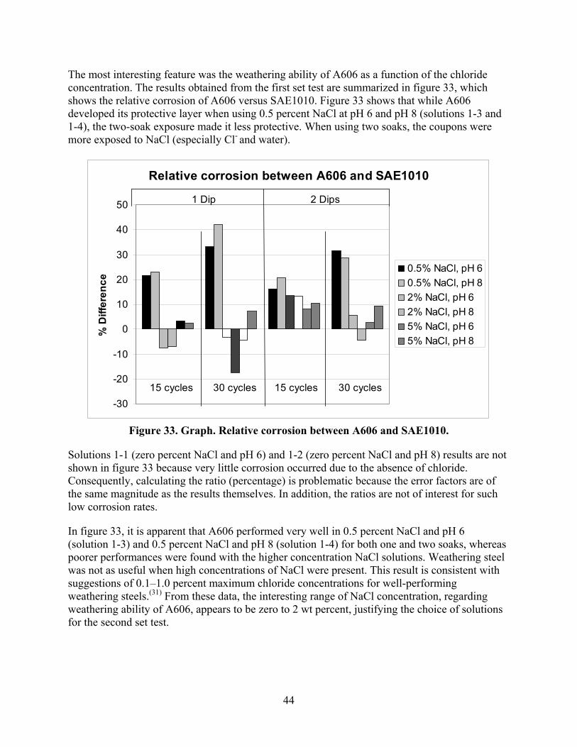
44

The most interesting feature was the weathering ability of A606 as a function of the chloride concentration. The results obtained from the first set test are summarized in figure 33, which shows the relative corrosion of A606 versus SAE1010. Figure 33 shows that while A606 developed its protective layer when using 0.5 percent NaCl at pH 6 and pH 8 (solutions 1-3 and 1-4), the two-soak exposure made it less protective. When using two soaks, the coupons were more exposed to NaCl (especially Cl- and water).

Relative corrosion between A606 and SAE1010

-30

-20

-10

0

10

20

30

40

50

% D

iffe

ren

ce

0.5% NaCl, pH 6

0.5% NaCl, pH 8

2% NaCl, pH 6

2% NaCl, pH 8

5% NaCl, pH 6

5% NaCl, pH 8

1 Dip 2 Dips

15 cycles 30 cycles 15 cycles 30 cycles

Figure 33. Graph. Relative corrosion between A606 and SAE1010.

Solutions 1-1 (zero percent NaCl and pH 6) and 1-2 (zero percent NaCl and pH 8) results are not shown in figure 33 because very little corrosion occurred due to the absence of chloride. Consequently, calculating the ratio (percentage) is problematic because the error factors are of the same magnitude as the results themselves. In addition, the ratios are not of interest for such low corrosion rates.

In figure 33, it is apparent that A606 performed very well in 0.5 percent NaCl and pH 6 (solution 1-3) and 0.5 percent NaCl and pH 8 (solution 1-4) for both one and two soaks, whereas poorer performances were found with the higher concentration NaCl solutions. Weathering steel was not as useful when high concentrations of NaCl were present. This result is consistent with suggestions of 0.1–1.0 percent maximum chloride concentrations for well-performing weathering steels.(31) From these data, the interesting range of NaCl concentration, regarding weathering ability of A606, appears to be zero to 2 wt percent, justifying the choice of solutions for the second set test.

45

Influence of pH

Two different pH values were selected to study pH’s influence on the corrosion of steel. Figure 34 through figure 37 present the corrosion values observed during the first set test. To clearly study pH’s influence, the only parameter varied in each graph was the pH of the solution used during the soaking process. Data after 15 and 30 cycles are presented.

Figure 34 through figure 37 suggest that regardless of the type of steel, wetting time (one or two soaks/cycle), or exposure time, a lower pH yields a slightly higher corrosion rate. The variation of the pH does not appear to have a critical role in the early corrosion stage when the corrosion value is slightly affected.

Regarding the weathering ability of A606, figure 38 suggests that pH had a stronger effect with low NaCl. Conversely, at a high concentration of NaCl (5 percent) and a high number of cycles (30), pH had no effect.

Figure 34. Graph. A606 corrosion as a function of chloride concentration during a

one soak/cycle exposure.

46

Figure 35. Graph. A606 corrosion as a function of chloride concentration during a

two soak/cycle exposure.

Figure 36. Graph. SAE1010 corrosion as a function of chloride concentration during a

one soak/cycle experiment.

47

Figure 37. Graph. SAE 1010 corrosion as a function of chloride concentration during a

two soak/cycle experiment.

Figure 38. Graph. Relative corrosion versus NaCl concentration during exposure to a

one soak/cycle environment.

Influence of Wetting Time

Environments including one soak/cycle and two soaks/cycle were used to study the influence of the wetting time on the corrosion of the steels and the weathering ability of A606. Results are presented in figure 39 through figure 42.

48

Figure 39. Graph. A606 corrosion as a function of chloride concentration at pH 6.

Figure 40. Graph. A606 corrosion as a function of chloride concentration at pH 8.

49

Figure 41. Graph. SAE1010 corrosion as a function of chloride concentration at pH 6.

Figure 42. Graph. SAE1010 corrosion as a function of chloride concentration at pH 8.

Figure 41 and figure 42 show that the wetting time with high NaCl concentrations had a strong effect on SAE1010 as well as A606. Values with two soaks were much greater than those with one soak, especially for pH 8. Considering pH 6, corrosion values were becoming similar for the highest NaCl percentage. Increased wetting time and higher NaCl concentration had less influence on corrosion. A possible explanation is that at a high NaCl concentration, the oxide layer was saturated with NaCl, and the additional NaCl did not cause further change. However, at a lower pH of 6, corrosion increased, which suggests that a lower pH had a synergistic effect with NaCl to further saturate the oxide layer with chloride.

50

Second Set Test

The complete set of data, which includes individual specimen dimensions and weights, is available.(33) An example calculation is given in the appendix for converting the data to units used in this report. Compilations of the data are presented in figure 43 and figure 44. The data are plotted and discussed as the average results of triplicate specimens unless stated otherwise.

Figure 43. Graph. Corrosion of A606 and SAE1010 versus chloride concentration for

the second test set.

Figure 44. Graph. Relative corrosion versus chloride concentration.

Based on the first set of test results, an interesting range of chloride concentration was determined for the soaking solution, which was greater than zero and less than 2 percent NaCl. In these tests, only pH 8 was used with chloride concentration (0.1–1.6 percent NaCl), which was the only factor that was varied.

51

Note that for 0.1–1.6 percent NaCl, the corrosion value of SAE1010 was always greater than the value of A606, meaning that in that range of concentration, weathering steel was performing as expected by forming a protective oxide.

A606 performed well for 15 cycles. For a NaCl concentration greater than 0.5 wt percent, the weathering ability after 30 cycles seemed to decrease. This decrease is observed in figure 44 where the 30-cycle data falls below that of the 15-cycle data. Issues might be encountered for longer exposure times because the corrosion rates for A606 increase for 30 cycles compared to 15 cycles.

XRD and Corrosion Rate

Several corrosion specimens were analyzed by XRD and correlated with their corrosion rates. The results are given in table 14 and discussed below. Table 14 presents the peaks and their intensities relative to the individual compound’s major peak. These are semiquantitative percentages and do not intend to represent a quantitative rust composition. The results give indications concerning the composition of the rust and can be related to the results found in field studies. Additional XRD analyses are discussed in chapter 8.

52

Table 14. Observed major peak intensities using XRD and corrosion rates.

Specimen Exposure

Description Corr. Rate

(mm/y) Goethite -FeOOH

Lepidocrocite -FeOOH

Maghemite -Fe2O3

Akaganeite -FeOOH

W67 (A606)

2 percent NaCl pH 8 1 soak 15 cycles 0.039 76.5 21.4 0 0

W23 (A606)

0.5 percent NaCl pH 8 1 soak 30 cycles 0.043 100 11 0 0

W88 (A606)

5 percent NaCl pH 8 1 soak 30 cycles 0.122 100 8.3 17.7 0

W70 (A606)

2 percent NaCl pH 8 2 soaks 30 cycles 0.140 100 14.1 42.9 0

070 (SAE1010)

2 percent NaCl pH 8 2 soaks 30 cycles 0.132 100 0 22.3 0

Weathering Steel—15-Cycle Exposure with Protective Patina

Coupon W67 was exposed to a solution of pH 8 containing 2 percent NaCl using one soak/cycle. Weight loss results showed that it developed a protective layer (see table 14).

The intensity peak was achieved by metallic iron (the substrate) at 44.7 degrees. The second peak of this pattern was at 21.7 degrees, which was the goethite strong peak. Its second strongest peak was present at 36.5 degrees. A small 27.8-degree peak indicated that lepidocrocite was present in the oxide layer.

Weathering Steel—30-Cycle Exposure with Protective Patina

Coupon W23 was exposed to a solution of pH 8 containing 0.5 percent NaCl using one soak/cycle. Weight loss results showed that it developed a protective layer (see table 14).

The peak with the highest intensity at 21.7 degrees corresponded to the goethite peak, which was 81 percent of the protective patina. The second peak was also identified at 36.3 degrees. Peaks at 14.8 and 27.6 degrees corresponded to lepidocrocite. These smaller peaks indicated that there was little of this crystal phase in the oxide layer.

53

Weathering Steel—30-Cycle Exposure with Nonprotective Patina Exposed to High Chloride Concentration

Coupon W88 was exposed to 5 percent NaCl using one soak/cycle. Weight loss results showed that it did not develop a protective layer (see table 14).

Goethite was the main constituent of the oxide layer with peaks at 21.6 and 36.3 degrees. An iron peak was also present at 44.9 degrees and was likely due to metallic iron particles being undermined from the surface by corrosion or from scraping the coupon surface to remove the oxide for analysis. A small amount of maghemite was identified at 63.5 degrees. The first two maghemite peaks may have coalesced with the 36.3-degree peak of goethite.

Weathering Steel—30-Cycle Exposure with Nonprotective Patina Exposed to High Time of Wetness

Coupon W70 was exposed to 2 percent NaCl at pH 8 using two soaks/cycle (see table 14). Weight loss results showed that it did not develop a protective layer.

Goethite was identified by its main peak at 21.5 degrees. Its second peak was also present at 36.19 degrees. The relatively high intensity peak at 63.3 degrees indicated that a large fraction of maghemite was present in the oxide layer. The first two peaks of maghemite coalesced with the 36.3-degree peak of goethite.

Carbon Steel—30-Cycle Exposure with Nonprotective Patina Exposed to High Chloride Concentration

Coupon 070 was exposed to 2 percent NaCl at pH 8 using two soaks/cycle (see table 14). Weight loss results showed that it did not develop a protective layer. Goethite was the main constituent of the oxide layer. Maghemite was also observed at 63.6 degrees.

Analyses of Carbon and Weathering Steel Corrosion Products

XRD analyses were made on corrosion products obtained from additional specimens after completion of the cyclic tests. These are discussed in the next section.

Summary of XRD Analysis

The XRD results obtained from the coupons tested in the accelerated exposure chamber were in general agreement with the field study results given in table 14.(24) High wetting time developed maghemite and lepidocrocite, while high chloride developed maghemite and sometimes akaganeite. Goethite was present in every corrosion product whether it was protective or not. Thus, increasing the concentration of chloride, providing additional chloride exposure (a second soak), and increasing the wetting time all had the same effect in the laboratory as in field exposure. For example, specimens W67 and W23 exhibited low corrosion relative to W88, W70, and 070. The conditions of 2 percent NaCl (or lower) with a single soak represented low chloride and relatively drier conditions for W67 and W23. Conversely, conditions of 2 percent NaCl (or higher) with two soaks represented higher chloride and wetness exposures.

54

The exposure chamber experiments produced results similar to those observed for steel in field exposure. Maghemite was found in almost all nonprotective corrosion products. One anomaly was the absence of akaganeite in the high chloride-soaked specimens, which may have been due to fresh water condensing humidity rinsing away chloride during the wet cycle portion. Generally, the laboratory tests were able to reproduce the conditions found during field exposure, especially with regard to high corrosion rate and maghemite correlation. Comparison of the laboratory and field exposures was not straightforward because the laboratory conditions could be controlled while the field conditions were dependent on natural (variable) environmental changes during the exposure.

TASK 2.2. CORROSION RATES OF ACCELERATED TEST SPECIMENS USING GALVANIC SENSORS

Reaction to Humidity and Salt Application

One of the successes of the sensor design described in the previous chapter was due to its very good response to humidity and NaCl. In figure 45, when the wet cycle began, the output immediately increased due to the completion of the current path, and the current was recorded by the data logger. The current remained stable during the time the metal was corroding; salt deposits and amorphous corrosion products were washed out by the ambient condensing humidity. Once the salt was applied, the current increased, responding to the corrosion rate of the material being exposed to a more aggressive environment. The wet stage occurred between the 6th and 12th hours, and soaking occurred at the 11th hour. After soaking the specimen, the dry cycle began, resulting in an increased current as the electrolyte layer dried. This increased the conductivity and infusion of oxygen through the thinner layer. When the drying was complete, the current dropped to zero. In the dry cycle, localized corrosion could occur as well as corrosion product crystallization and resizing of the crystallites.

Sensor output for the 15-cycle exposures is presented in figure 46. During the eighth cycle, the wet stage did not start because of an experimental chamber failure. The salt soaking was still performed, and each sensor responded the same way but with differing magnitudes. The outputs had the shape of a spike corresponding to the time needed for the salt solution to dry in the chamber. This unplanned event shows the reproducibility of the output for a given event over the whole sensor population, showing another success for the sensors. In the figure, D-W indicates approximate dry-wet periods.

55

24h cycle sensor 1-C-W

010203040

5060708090

1 2 3 4 5 6 7 8 9 10 11 12 13 14 15 16 17 18 19 20 21 22 23 24

Time (Hours)

Cu

rren

t (

A)

Wet stage

Soaking in salt

Figure 45. Graph. Output for a Cu-A606 atmospheric corrosion sensor using

soaking solution 3-1.

Output for Sensor C-W using Solution 3-1

0

20

40

60

80

100

120

0 20 40 60 80 100 120 140 160 180 200 220240 260 280 300 320 340 360 380 400

Time (Hours)

Cu

rren

t (µ

A)

Figure 46. Graph. Output for Cu-A606 sensor during a 15-cycle test.

The output for the last three cycles after the weekend break was also interesting. Current readings dropped for each kind of steel, even more for A606. In the standard SAE J2334, the weekend break was optional. The reason why the corrosion rate decreased may be related to the crystallization time needed for the oxides to form. Oxides that constitute the protective layer needed to crystallize during the dry stage. If the dry stage was too short, the final crystallographic reformation was not complete, and consequently the protective layer was not completely formed. It is known that weathering steel requires dry and wet cycles to perform well, but the time required has not been characterized. If a corrosion performance test is to be developed further, drying time during weekends should be required or perhaps extended. Other data support this last statement. For the first set test (weight loss coupons), six weekend dry stages were performed, whereas for the second set test, only two weekend breaks were performed. By combining data obtained with the two exposure tests (see figure 40 and figure 43), figure 47 was created.

D-W-D-W-D-W-D-W-D-W-D-W-D-W-D-W-D-W-D-W-D-W-----D-----W-D-W-D-W-D

56

Corrosion of A606 as a function of NaCl concentration

0

0.02

0.04

0.06

0.08

0.1

0.12

0.14

0 1 2 3 4 5 6

NaCl wt%

Cor

rosi

on

Pe

netr

atio

n (m

m)

15 cycles

30 cycles

Figure 47. Graph. Corrosion of A606 versus NaCl concentration.

In figure 47, the corrosion value dropped between 1.6 and 2.0 wt percent NaCl. The data for 1.6 wt percent concentration was from the second set test, whereas the data for 2.0 wt percent concentration was from the first set test. The drop was due to the option of the experimental protocol that was not supposed to have a significant effect on the results according to standard SAE J-2334. The results show that drying time was an important factor when dealing with the corrosion of weathering steel. Weekend drying time should be included in the standard and should be a topic for additional study. The role of drying time was easily studied by cyclic coupon and sensor tests.

Corrosion Rate Determination

The sensors were intended to provide information about the corrosion rate of the material from which they were fabricated. To verify that the output of the sensors represents the actual corrosion rate in the same environment, the output of the sensors can be compared (see table 15) with the results obtained during the exposure of the coupons.

By integrating microamperes over the time, coulombs (i t = C) are found, which are related to weight loss using Faraday’s law. All microampere readings were averaged by the data logger over the sampling time of 1 hour (3,600 s). An example calculation is given in the appendix.

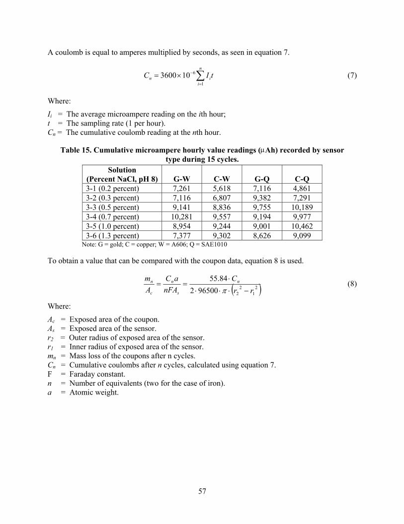
57

A coulomb is equal to amperes multiplied by seconds, as seen in equation 7.

tICn

iin

1

6103600 (7)

Where:

Ii = The average microampere reading on the ith hour; t = The sampling rate (1 per hour). Cn = The cumulative coulomb reading at the nth hour.

Table 15. Cumulative microampere hourly value readings (Ah) recorded by sensor type during 15 cycles.

Solution (Percent NaCl, pH 8) G-W C-W G-Q C-Q 3-1 (0.2 percent) 7,261 5,618 7,116 4,861 3-2 (0.3 percent) 7,116 6,807 9,382 7,291 3-3 (0.5 percent) 9,141 8,836 9,755 10,189 3-4 (0.7 percent) 10,281 9,557 9,194 9,977 3-5 (1.0 percent) 8,954 9,244 9,001 10,462 3-6 (1.3 percent) 7,377 9,302 8,626 9,099

Note: G = gold; C = copper; W = A606; Q = SAE1010

To obtain a value that can be compared with the coupon data, equation 8 is used.

21

22965002

84.55

rr

C

nFA

aC

A

m n

s

n

c

n

(8)

Where:

Ac = Exposed area of the coupon. As = Exposed area of the sensor. r2 = Outer radius of exposed area of the sensor. r1 = Inner radius of exposed area of the sensor. mn = Mass loss of the coupons after n cycles. Cn = Cumulative coulombs after n cycles, calculated using equation 7. F = Faraday constant. n = Number of equivalents (two for the case of iron). a = Atomic weight.

58

Plotting the sensor data and the coupons data gives figure 48 and figure 49. For both figures, the dashed boxes identify over-range sensor data.

Figure 48. Graph. Corrosion (weight loss) of A606 coupons and calculated mass-loss for

A606 sensors versus NaCl concentration for 15-cycle exposure.

Figure 49. Graph. Corrosion (weight loss) of SAE1010 coupons and calculated mass-loss

for SAE1010 sensors versus NaCl concentration for 15-cycle exposure.

For A606 steel (see figure 45), corrosion values calculated from the sensors were lower than those from the weight loss experiment (even after applying a 2X factor). However, the first three data points of sensors and coupons followed the same trend. The trend indicated that the more chlorides present in the solution, the higher the corrosion value. The last three (higher) concentrations reached a maximum corrosion value for the sensors. An explanation is that the output was off-scale, as can be seen on the sensors’ output data. The amperes or coulombs obtained reached the maximum value (scale) that the data logger could record, indicated by a plateau with increasing chloride concentration. Consequently, those six data points (three for the G-W sensors and three for the C-W sensors) were invalid and should not be compared to weight loss data.

The same phenomena occurred for the SAE1010 sensors output. These sensors indicated that sensors made of SAE1010 were providing higher output values than (higher corrosion rate) that those made of A606. The higher rate was inferred by the coulomb values achieving maximum (plateau) values at lower chloride concentrations in figure 48 and figure 49 or higher values in table 15, especially for the copper cathode sensors. This result was reasonable due to the weathering ability of A606. Above a chloride concentration of 0.7 wt percent, the sensors

59

produced an off-scale output that was invalid for quantitative comparisons. The first three sensor data points for both A606 and SAE1010 followed the trend of the coupon data where higher NaCl concentration indicated a higher corrosion value.

In general, sensors were able to indicate the corrosion rate of material exposed to the same environment, although a scale (proportionality) problem should have been considered. The sensors were sensitive to chloride concentration. A smaller active anode area or a wider range data logger is suggested for future studies. Table 15, figure 48, and figure 49 suggest that copper cathodes provide more consistent results than the gold cathodes.

RESULTS OF TASK 2.3. PROTOTYPE CABLE CORROSION SENSORS

The main sources of moisture for cables are rainwater and condensation. These moistures are often mimicked by dilute Harrison solution for corrosion testing.(33) The solution contains ammonium sulfate and NaCl usually found in atmospherically deposited moisture.

Cable Sensor Response to Test Conditions

Cyclic

Figure 50 presents the sensor responses of dry specimens exposed to SAE J2334 cyclic conditions (except no soaking) followed by a experiencing a single soak in dilute (1/10 concentration) Harrison solution after 32 days and continuing the cycling without additional soaks. In each case, the sensors yielded little or no response until wetted by the dilute Harrison solution after 32 days. Each sensor showed a large increase in response after wetting. The responses observed were expected for wetted sensors. The specific nature of the response varied somewhat depending upon wetness saturation of the sensor within the specimen. In figure 50, the large response after wetting was followed by a large decrease corresponding to drying of the sensor. Subsequently, small responses that corresponded to the high humidity phase in the exposure chamber were observed every 24 hours.

Figure 50. Graph. Response of cable sensor before and after dilute Harrison solution.

60

Soaked

Figure 51 presents typical cable sensor responses of specimens soaked for 15 minutes in dilute (1/10 concentration) Harrison solution followed by equilibration under static conditions of 50 percent RH. Figure 52 presents the typical responses for similar tests for 100 percent RH. The responses showed that the more tightly wrapped specimens and those under the higher relative humidity maintained higher levels of current for longer times than loosely wrapped specimens or those under lower RH. These responses were consistent with corrosion that occurred in the presence of sufficient moisture.

Figure 51. Graph. Response of cable sensor during constant 50-percent RH exposure after

dilute Harrison solution.

Figure 52. Graph. Response of cable sensor during constant 100-percent RH exposure after

dilute Harrison solution.

61

XRD Results for Cable Test Specimens

Table 16 and figure 53 show the XRD results for the corrosion products that were obtained from the cable specimen rods. The most notable difference compared to the coupon materials was the presence of butlerite. Butlerite is a ferrihydroxysulfate compound, and its formation is due to the presence of sulfate from the dilute Harrison solution used to wet the sensors.

62

Table 16. Percentage corrosion components in specimens determined by XRD.

Condition

Specimen 0 = SAE1010,

W = A606 Percent Goethite

Percent Maghemite

Percent Lepidocrocite

Percent Other

024 40 60 — — 041 43 57 — — 042 46 54 — — 060 61 39 — — 063 48 52 — — 069 — 74 — 26 Hematite 072 20 65 15 — W63 40 29 31 —

1-soak

W69 37 32 31 — 021 43 57 — — 024 28 40 32 — 032 56 44 — — 035 42 58 — — 038 41 31 28 — 041 24 76 — — 042 45 55 — — W01 20 80 — — W09 56 — 44 — W21 37 37 26 — W24 24 45 31 — W33 59 — 41 — W35 35 65 — — W38 25 41 34 —

2-soak

W48 44 56 — — L1C 15 16 25 44 Butlerite L2C 15 22 23 40 Butlerite L3C 15 13 26 46 Butlerite T1C 8 27 15 50 Butlerite T2C 12 24 12 52 Butlerite

Cable specimen rods near sensors (see table 11)

T3C 19 45 17 19 Butlerite The bolded text, “0,” represents SAE1010 material. — Indicates that data was not found. L = loose wrap. T = tight wrap. C = cyclic exposure.

63

Figure 53. Graph. XRD pattern of steel rods in cable sensor bundle after single soak in

dilute Harrison solution and exposure in cyclic chamber for 40 days.

65

CHAPTER 9. RESEARCH STUDY #2 FINDINGS

There are several findings from the second research study, which include the following:

An accelerated corrosion test was developed for weathering steel corresponding to a range of exposure conditions that demonstrated sensitivity to chloride environments.

The protective oxide layer (patina) of weathering steel was degraded above 0.5 wt percent chloride. Above 1 wt percent chloride, the protective oxide was severely degraded.

Sensors were able to indicate the corrosion rate of coupon material exposed to the same environment.

Sensors allowed direct and immediate observation of the impact that environmental changes had on corrosion rate.

XRD showed that the corrosion products produced in cycle test chambers were similar to those observed under field conditions.

Bridge cable sensors were developed which were capable of monitoring corrosive conditions within suspension bridge cables and other occluded geometries.

67

CHAPTER 10. CONCLUSIONS

The findings of both research studies comprise the following general conclusions of this report:

Exposure of U-bend specimens fabricated from 16-mm-diameter 2304 SS to simulate pore solution with chlorides at ambient temperature and 65 oC failed to reveal any susceptibility to stress corrosion cracking.

The critical chloride concentration required to initiate the corrosion of 2304 SS specimens polarized to +100 mVSCE while exposed to simulated pore water to which chlorides were incrementally added ranged from 5.00–9.86 wt percent Cl-.

No definitive corrosion initiation occurred after 929 days for three concrete slab specimens with 2304 SS reinforcement that were ponded with a Cl- solution. For one specimen, some momentary activity followed by repassivation occurred.

The Cl- threshold to initiate active corrosion of 2304 SS in concrete was greater than 12.5 kg/m3 (4.51 wt percent cement).

An accelerated corrosion test was developed for weathering steel corresponding to a range of exposure conditions that demonstrated sensitivity to chloride environments.

The protective oxide layer (patina) of weathering steel was degraded above 0.5 wt percent chloride. Above 1 wt percent chloride, the protective oxide was severely degraded.

Sensors indicated the corrosion rate of coupon material exposed to the same environment.

Sensors allowed direct and immediate observation of the impact of environmental changes on corrosion rate.

XRD showed that the corrosion products produced in cycle test chambers were similar to those observed under field conditions.

Bridge cable sensors were capable of monitoring corrosive conditions within suspension bridge cables and other occluded geometries.

69

APPENDIX

CALCULATIONS

In this appendix, calculations that were used to convert laboratory measurements to units in text, tables, and graphs are provided as examples.

Example 1. Convert Weight/Area (Corrosion in g/inches2) to mils (or mm) Corrosion Penetration

Data for specimen W48: test condition was 30 cycles, 2 soaks, 0.5 percent NaCl, and pH 8.

Typical Data Weight (Initial)

Weight (Final)

Area (L by W2)

Corrosion ( wt/inches2 )

Coupon W48 124.90766 g 119.02947 g 34.16 inches2 0.1721 g/inches2

1 inch = 25.4 mm 1 oz = 28.35 g

Convert to centimeters:

222

2

2 /02667.054.2/154.2

/1721.0 cmgcmgcm

ining

(9)

Convert weight per surface area to penetration (divide by density):

cmcmgcmg 00339.0/87.7/02667.0 32 (10)

Also:

0.00339 cm 10 mm/cm = 0.0339 mm (11) Convert to mils (1 inch = 1,000 mils):

milsin

mils

cm

incm 33.1

1000

54.200339.0 (12)

These are the penetration rates in mm, m, cm, or mils for corrosion occurring on one surface. In the case of corrosion occurring on both sides, the overall thickness loss would be doubled.

70

Example 2. Conversion of ZRA Current to Coulombs

)( CsACti (13)

Where:

I = Current. t = Time. A = Amperes. s = Seconds. C = Coulombs.

ZRA data logger recorded averaged current (i) each hour.

The eight-bit analog-to-digital converter stored the sum of six readings in hexadecimal format, that is, the summed eight-bit readings (0 to 255 hex) were summed to give a value between zero and 05 FA (hex) and stored.

Stored data were downloaded from the logger to the computer. Scaling was 255 (hex) = 100 μ A (full-scale).

Microsoft Excel® macro converted hexadecimal to decimal, divided by 6, and scaled by 100/255.

The result was μ A average current reading per hour.

The Microsoft Excel® macro also summed the hourly average current readings (in microamperes) and multiplied them by 3,600 s to yield microcoulombs (i t = C).

Example: For constant, half-scale readings (50 μA) for 15 days converted to coulombs:

Ch

s

day

hdays

sA

CAC 8.64

360024151050# 6

(14)

Note that the data logger recorded a value equal to an average current value each hour. In this example, 0.18 C was measured each hour. Summing (integrating) these hourly values for 15 days yielded 64.8 C.

71

Example 3. Conversion of Sensor Output (μA) to Corrosion Rate (mpy or mmpy)

Faraday’s Law of Electrolysis:

nF

Itam (15)

Where:

m = Mass (g). I = Current (A). t = Time (s). a = Atomic weight; (g). n = Number of equivalents, eq, (number of electrons exchanged, for Fe = Fe2+ + 2e- ). F = Faraday’s constant, 96,500 C per equivalent. For 1 μ A output per year (recall that C=A s):

geqCmoleeq

molegsA

nF

Itam 0091.0

)/500,96)(/2(

)/8.55)(1015.3)(10( 76

(16)

For 1 μ A output in an area of 1 cm2 and given an iron density of 7.87 g/cm3:

mmpympyin

mils

cm

in

g

cm

cm

gcmA 012.046.0

1000

54.287.70091.0/1

3

22 * (17)

1 mpy = 0.0254 mmpy * Indicates same result as in D. Jones.(34)

Equation 17 demonstrates the conversion of constant or average current density to mils per year or mm per year. The data logger provided the average of six current measurements at 10-minute intervals each hour. These hourly averages are summed and presented in table 15.

Example 4. Comparison of Mass Loss and Sensor Results in Terms of Penetration

For reference for this example, refer to figure 48 and figure 49. For the ATM sensor, the sensor anode area, the location where mass loss occurred, and the mass corresponding to coulombs obtained with the data logger must be calculated.

Sensor anode area is the two-dimensional ring between the inner washer, r1 , and the outer coated perimeter, r2:

222

2221

22 58.1504.0

54.2250.0375.0 cmcm

in

cmininrrAsensor

(18)

To calculate the mass loss from the downloaded converted sensor output (microamperes), substitute C = A s, (i.e., replace It in equation 15 with the coulomb value). For example, use

72

the first value (7,261 μ A) in table 15 that is an hourly value requiring conversion to seconds (1 h = 3,600 s) as follows:

geqCmoleeq

moleghsAh

nF

Itam 0076.0

)/500,96)(/2(

)/8.55)(/3600)(107261( 6

(19)

The calculated mass loss per unit area of the sensor anode is converted to penetration using the density of iron as follows:

mmcm

mm

g

cm

cm

g0061.0

10

87.758.1

0076.0 3

2 (20)

For the cable sensor, no direct comparison with weight loss was possible with the available data. An estimate of corrosion rate (penetration) was made based on sensor area and current output.

Area calculation where:

Anode wire diameter = 0.08 cm. Active length = 2.5 cm. Anode area is dl = 3.14 0.08 cm 2.5 cm = 0.63 cm2. Sensor output:

From equation 17, 1 μ A/cm2 = 0.46 mpy. For a 0.63-cm2 sensor giving a current reading of 1 μ A, the current density is (1 μ A / 0.63 cm2) = 1.6 μA / cm2, and a sensor reading of 1 μA corresponds to 0.74 mpy as follows:

xmpy

AA 46.0

6.11 , x = 0.74 mpy (21)

73

REFERENCES

1. Virmani, Y.P, Jones, W.R., and Jones, D.H. (1984). “Steel Corrosion in Concrete: pH at Corrosion Sites,” Public Roads, 84(3), 96.

2. Koch, G.H., Brongers, P.H., Thompson, N.G., Virmani, Y.P, and Payer, J.H. (2002). Corrosion Costs and Prevention Strategies in the United States, FHWA-RD-01-156, Federal Highway Administration, Washington, DC.

3. Yunovich, M., Thompson, N.G., and Virmani, Y.P. (2003). Life Cycle Cost Analysis for Reinforced Concrete Bridge Decks, Paper No. 03309, Presented at CORROSION/03, San Diego, CA.

4. Stratfull, R.F., Jurkovich, W.J., and Spellman, D.L. (1975). “Corrosion Testing of Bridge Decks,” Transportation Research Record 539, 50, Transportation Research Board, Washington, DC.

5. Code of Federal Regulations Section 650.305. (2002). Frequency of Inspections, U.S. Government Printing Office, Washington, DC.

6. Stafford, R.T. (1973). “Epoxy Coated Rebars,” Parking, 39.

7. Clifton, J.R., Beehgly, H.F., and Mathey, R.G. (1974). Non-Metallic Coatings for Concrete Reinforcing Bars, FHWA-RD-74-18, Federal Highway Administration, Washington, DC.

8. Virmani, Y.P. and Clemena, G.G. (1998). Corrosion Protection: Concrete Bridges, FHWA-RD-98-088, Federal Highway Administration, Washington, DC.

9. Powers, R.G. and Kessler, R. (1987). Corrosion Evaluation of Substructure, Long Key Bridge, Corrosion Report No. 87-9A, Florida Department of Transportation, Gainesville, FL.

10. Powers, R.G. (1988). Corrosion of Epoxy-Coated Rebar, Keys Segmental Bridges Monroe County, Report No. 88-8A, Florida Department of Transportation, Gainesville, FL.

11. Zayed, A.M. and Sagűés, A.A. (1989). Corrosion of Epoxy-Coated Reinforcing Steel in Concrete, Paper No. 386 presented at CORROSION/89, New Orleans, LA.

12. Gustafson, D.P. (1988). “Epoxy Update,” Civil Engineering, 58(10), 38.

13. Federal Highway Administration. (1989). Technical Advisor—Uncoated Weathering Steel In Structures, T 5140.22, Federal Highway Administration, Washington, DC.

14. Granata, R.D, Fisher, J.W., and Wilson, J.C. (1997). Update on Applications of Corrosion Coulometers, Paper 97307, CORROSION/97 Conference, NACE International, Houston, TX.

15. Granata, R.D. and Madani, M.M. (1997). SAE International Congress and Exposition, Paper No. 970736, Society of Automotive Engineers, Detroit, MI.

74

16. Yu, H. and Hartt, W.H. (2007). “Effect of Reinforcement and Coarse Aggregates on Chloride Ingress into Concrete and Time-to-Corrosion: Part I—Spatial Chloride Distribution and Implications,” Corrosion, 63, 843.

17. Yu, H., Himiob, R.J., and Hartt, W.H. (2007). “Effect of Reinforcement and Coarse Aggregates on Chloride Ingress into Concrete and Time-to-Corrosion: Part II—Spatial Distribution of Aggregates,” Corrosion, 63, 924.

18. Hartt, W.H. and Nam, J. (2008). Effect of Cement Alkalinity Upon Chloride Threshold and Time-to-Corrosion of Reinforcing Steel in Concrete, Paper No. 08322, Presented at CORROSION/08, NACE International, Houston, TX.

19. Hartt, W.H., Powers, R.G., Presuel-Moreno, F., Paredes, M., Simmons, R., Hui, Y., Himiob, R., and Virmani, Y.P. (2009). Corrosion-Resistant Alloys for Reinforced Concrete, FHWA-HRT-09-020, Federal Highway Administration, Washington, DC.

20. Florida Department of Transportation. (1994). Florida Method of Test for Determining Low-Levels of Chloride in Concrete and Raw Materials, Designation FM 5-516, Florida Department of Transportation, Tallahassee, FL.

21. Sagűés, A.A. (2003). “Modeling the Effects of Corrosion on the Lifetime of Extended Reinforced Concrete Structures,” Corrosion, 59, 854.

22. ASTM International. (2004). “Standard Guide for Estimating the Atmospheric Corrosion Resistance of Low-Alloy Steels,” Annual Book of ASTM Standard, 03.02, ASTM G101-04, ASTM International, West Conshohocken, PA.

23. ASTM International. (2002). “Specification for Steel Wires, Music Spring Quality,” Annual Book of ASTM Standard 01.02, ASTM A228, ASTM International, West Conshohocken, PA.

24. SAE International. (2003). Lab Cosmetic Corrosion Test, SAE J2334, Society of Automotive Engineering Surface Vehicle Standard, SAE International, Warrendale, PA.

25. Repp, J. (2002). “Update on the Development of SAE J2334 Accelerated Corrosion Test Protocol,” U.S. Army Corrosion Summit, St. Petersburg, FL.

26. ASTM International. (2003). “Standard Practice for Preparing, Cleaning, and Evaluating Corrosion Test Specimens,” Annual Book of ASTM Standard, 03.02, ASTM G1-03, ASTM International, West Conshohocken, PA.

27. Cook, D.C., Oh, S.J., and Townsend, H.E. (1998). The Protective Layer Formed on Steels After Long-Term Atmospheric Exposure, Paper No. 98343, NACE International, Houston, TX.

28. Downs, R.T. and Hall-Wallace, M. (2003). “The American Mineralogist Crystal Structure Database,” American Mineralogist, 88, 247–250.

75

29. White, M.L. and Leidheiser Jr., H. (1990). “The Corrosion Coulometer—A New Corrosion Monitor for Steel Structures,” Corrosion, 46(8), 653–661.

30. Granata, R.D., Michalerya, W.D., Wildt, R.H., Leidheiser Jr., H, and O’Malley Jr., B.W. (1992). “Quantitative Evaluation of Steel Corrosion in Microenvironments Using the Corrosion Coulometer,” Review of Progress in Quantitative Nondestructive Evaluation, 11, 1183–1190, Plenum Press, New York, NY.

31. Héreng, Y. (2007). Atmospheric Corrosion Study of Weathering Steel Using Sensor Technology, Florida Atlantic University, Boca Raton, FL.

32. Cook, D.C. and Granata, R.D. (2002). NYS DOT Moore Drive Bridge: Coupon Exposure Project, Interim Report #1, Specimen Rack Construction and Installation, Report No. T:202, American Iron and Steel Institute, Washington, DC.

33. ASTM International. (1994). Standard Practice for Modified Salt Spray (Fog) Testing, Annex 5, ASTM G 85-94, West Conshohoken, PA.

34. Jones, D. (1996). Principles and Prevention of Corrosion, 2nd ed., Prentice-Hall, Upper Saddle River, NJ.

HRDI-10/10-09(500)ERecycledRecyclable