integration of sample design for the national survey … · integration of sample design for the...

Integration ofSample Design forthe National Surveyof Family Growth,Cycle IV, With theNational HealthInterview SurveyResearch was undertaken to develop

alternative methods of selecting a sample

of eligible women for the National Survey

of Family Growth (NSFG) from the National

Health Interview Survey (N HIS). This

report presents estimates of the effects

of alternative design options, obtained by

statistical modeling techniques, for linking

the NSFG with the NH IS. The estimated

survey costs, lengths of data collection

period, and projected response rates for

alternative linked design options and for

the unlinked design are compared for fixed

precision. The findings indicate that

substantial gains in the NSFG design

efficiency could be realized if particular

linked design options are adopted to

replace the independent design.

Data Evaluation and MethodsResearch

Series 2, No. 96

DHHS Publication No. (PHS) 86–1370

U.S. Department of Health and Human

Services

Public Health Service

National Center for Health Statistics

Hyattsville, Md.

December 1985

Copyright Information

All material appearing In thts report is In the public domain and may

be reproduced or copted wtthout permws!on; c{tatlon as to source,

however, is appreciated.

Suggested Citation

National Center for Health Statlstlcs, J. Waksberg and D. R. Northrup:

Integration of sample design for the National Survey of Fam!ly Growth,

Cycle IV, with the National Health Interview Survey. Vita/ and Hea/th

.Watkfics. Series 2, No. 96. DHHS Pub. No. (PHS) 86–1370. Public

Health Service. Washington. U.S. Government Printing Office,

Dec. 1985,

Library of Congress Cataloging-in- Publication Data

Waksberg, Joseph.

Integration of sample design for the National

Survey of Family Growth, Cycle IV, with the National

Health Interview Survey.

(Vital & Health Statistics. Series 2, Data evaluation

and methods research ; no. 96) (DHHS publication ; no.

(PHS) 86-1370)

Written by Joseph Waksberg and Doris R, Northrup.

Supt. of Dots. no.: HE 20.6209:2/96.

1. Family size—United States—Statlstlcal methods.

2. Fertlltty, Human—United States. 3. Birth control—

United States, 1. Northrup, Doris R. Il. National

Survey of Faintly Growth (U. S.) Ill. National Health

Interview Survey (U. S.) IV, National Center for Health

Statistics (U. S.) V. Title. V1. Series: Vital and

health statistics, Series 2, Data evaluation and

methods research ; no. 96. VII, Series: DHHS

publication ; no. (PHS) 86-1370. [DNLM: 1. Health

Surveys. 2, Research Design. 3. Sampling Studies.

4. Statistics. 5. Women. W2 A N148vb no.96]

RA409. U45 no. 96 312’.0723 S 84-600398

[HQ766.5,U] [306.8’5]

ISBN 0-8406-0311 -B

Foraale bythe Superintendent of Documents, U. S. Government Printing Office, Washington, D. C. 20402

National Center for Health Statistics

Manning Feinleib, M. D.. Dr. P. H., Director

Robert A. Israel, Deputy Director

Jacob J. Feldman, Ph. D., .4ssociate Director for Analysisand Epidem iolog]’

Garrie J. Losee, Associate Director for Data Processingand Services

Alvan O. Zarate, Ph. D., .4ssistant Director for InternationalStatistics

E. Earl Bryant, Associate Director for Interview andExamination Statistics

Stephen E. Nieberding. Associate Director for Management

Gail F. Fisher, Ph. D., Associate Director for ProgramPlanning, Evaluation, and Coordination

Monroe G. Sirken. Ph.D., Associate Director for Researchand Methodolog~’

Peter L. Hurley, Associate Director for Vital and HealthCare Statistics

Alice Haywood, Information Officer

Office of Research and Methodology

Monroe G. Sirken, Ph. D., Associate Director

Kenneth W. Harris, Special Assistant for ProgramCoordination and Statistical Standards

Robert J. Casady, Ph.D., ChieJ Statistical Methods Staff

James T. Massey, Ph.D+ ChieJ Survey Design Stafl

Symbols

. . . Data not available

,.. Category not applicable

Quantity zero

0.0 Quantity more than zero but less than

0.05

z Quantity more than zero but less than

500 where numbers are rounded to

thousands

*Figure does not meet standard of

reliability or precision

# Figure suppressed to comply with

confidentiality requirements

I iv

Several years ago the National Center for Health Statistics(NCHS) embarked on a long-range program to integrate the

designs of its national household sample surveys, including theNational Health Interview Survey (NHIS), the National Surveyof Family Growth (NSFG), the National Medical ExpenditureSurvey (NMES), and the National Health and Nutrition Ex-

amination Survey (NHANES). Each had been originally de-

signed and conducted as an independent survey with the U.S.Bureau of the Census serving as the NCHS collection agent forNHIS, and consulting firms in the private sector serving as the

collection agents for the other surveys.The basic concept of the proposed integrated design strategy

is that NHIS serve as the sampling frame for each of the other

NCHS household surveys. This design strategy appears to offer

opportunities for substantial gains in the overall design ef-ficiency of the integrated surveys. NHIS is by far the largest ofthe surveys, and it collects a wealth of household informationthat would be available for designing the samples for the other

surveys. However, this strategy would not have been feasibleprior to 1985, the year in which the most recently redesigned

NHIS was fielded. In prior years, decennial population listingsserved as one of the sampling frames for NHIS, and, therefore,

access to the personal identifiers of the sample households wasprohibited by the U.S. Bureau of the Census confidentiality

restrictions imposed by the law (13 U.S.C. 8,9), Beginning in

1985, however, this restriction no longer applies because theredesigned NHIS is based solely on an area sampling framewithout any use of decennial U.S. Bureau of the Census listings.

A research program is currently underway to evaluate the

effects on sampling errors, response rates, respondent burdens,timeliness, and so forth of linking the designs of NSFG,

NMES, and NHANES with NHIS. This research is intendedto provide answers to two questions:

1. Should the NCHS independently designed household sur-veys be replaced by an integrated survey design?

If question 1 is answered affirmatively, then,

2. What kind of integrated survey design should NCHS adopt?

In carrying out this research program the questions posedwill be addressed separately for the NSFG, NMES, and

NHANES because each survey involves its own unique linked

(integrated) design issues. However, a similar tw~phase re=search strategy will be followed in each case. First, statisticalmodeling techniques will be used to obtain provisional estimates

of the effects of alternative linked survey design strategies. Inthese investigations the unlinked design will be used as thestandard for comparison. Subsequently. the most promisinglinked survey design options will be verified and refined by

field testing. Finally, the design effects of the field-tested linkedsurvey design options will be evaluated.

This publication presents provisional estimates of the ef-

fects of alternative design options for linking the NSFG with

the NHIS that were obtained by statistical modeling techniques.The estimated survey costs, lengths of the data collection period,and projected response rates for alternative linked design optionsand for the unlinked design are compared for fixed precision.

The findings are quite encouraging and indicate that substantialgains in the NSFG design efficiency could be realized if par-

ticular linked design options are adopted to replace the in-

dependent design.

I provided technical oversight to Westat, Inc., the contractoron this study. I commend them and, in particular, Joseph

Waksberg and Doris Northrup for a job well done. A number

of NCHS staff participated in this project. Dr. Andrew Whiteconducted the technical review of this report. He worked closelywith the authors in making technical revisions and also workedwith the publications unit in making editorial revisions. Without

his endeavor this report would not have appeared in the Vitaland Health Statistics Series. Robert Fuchsberg, Director,Division of Health Interview Statistics, and Dr. William Pratt,Chief, Family Growth Branch, deserve special acknowledg-

ment. Without their full support and cooperation this projectwould not have been possible.

Monroe G. Sirken

Associate Director for Research and Methodology

Ill

Tables

14. Number of women 15–44 years, percent never married, and number never married, by age and race, 1981 and 1987projections . . . . . . . . . . . . . . . . . . . . . . . . . . . . . . . . . . . . . . . . . . . . . . . . . . . . . . . . . . . . . . . . . . . . . . . . . . . . . . . . . . . . . . . . . . . .

15. Eligible women, number of households, and households per eligible woman, by race and marital status, percent eligiblewomen retained afterlossin multieligible households, 1987 projections . . . . . . . . . . . . . . . . . . . . . . . . . . . . . . . . . . . . . . . . .

16. Parameters for estimation ofbetween-PSU effectby number ofPSU’s, race, and marital status . . . . . . . . . . . . . . . . . . . . .17. Values of(Z–l)pz bynumberofyears ofNHIS, race, andmarital status . . . . . . . . . . . . . . . . . . . . . . . . . . . . . . . . . . . . . . .18. Mobility rates forselectedpopulation groups, 1975-80 . . . . . . . . . . . . . . . . . . . . . . . . . . . . . . . . . . . . . . . . . . . . . . . . . . . . . . .19, Design effect components arising from subsampling housing units without eligible women in NHISby race and marital

status, . . . . . . . . . . . . . . . . . . . . . . . . . . . . . . . . . . . . . . . . . . . . . . . . . . . . . . . . . . . . . . . . . . . . . . . . . . . . . . . . . . . . . . . . . . . . . . . .20. Total design effects with alternative sample designs by race andmarital status . . . . . . . . . . . . . . . . . . . . . . . . . . . . . . . . . . .

Chapter 6: Sample sizes foraltemative designs . . . . . . . . . . . . . . . . . . . . . . . . . . . . . . . . . . . . . . . . . . . . . . . . . . . . . . . . . . . . . . . . .Sample sizes needed for specified reliability . . . . . . . . . . . . . . . . . . . . . . . . . . . . . . . . . . . . . . . . . . . . . . . . . . . . . . . . . . . . . . . . . .Sample size available fromNHIS forthe alternative designs . . . . . . . . . . . . . . . . . . . . . . . . . . . . . . . . . . . . . . . . . . . . . . . . . . . .Number ofyears ofNHIS required to provide needed sample size.. . . . . . . . . . . . . . . . . . . . . . . . . . . . . . . . . . . . . . . . . . . . . .Sample design for alternatives using sample ofpersons . . . . . . . . . . . . . . . . . . . . . . . . . . . . . . . . . . . . . . . . . . . . . . . . . . . . . . . . .Sample design for alternatives using sample ofhousingunits . . . . . . . . . . . . . . . . . . . . . . . . . . . . . . . . . . . . . . . . . . . . . . . . . . . .Screening workload with sample ofhousing units . . . . . . . . . . . . . . . . . . . . . . . . . . . . . . . . . . . . . . . . . . . . . . . . . . . . . . . . . . . . . .Sample size foralternative ofasampleoflO,OOO womenwithCycle III sample design . . . . . . . . . . . . . . . . . . . . . . . . . . . . . .Trackingworkload with one-time versus continuous data collection . . . . . . . . . . . . . . . . . . . . . . . . . . . . . . . . . . . . . . . . . . . . . .

Tables

21. Sample sizes required forequal reliability with alternative sample designsby race and marital status . . . . . . . . . . . . . . . . .22, Sample sizes ofhouseholds andeligible women available fromNHIS foraltemative sample designs byrace andmarital

status ofeligiblewomen. . . . . . . . . . . . . . . . . . . . . . . . . . . . . . . . . . . . . . . . . . . . . . . . . . . . . . . . . . . . . . . . . . . . . . . . . . . . . . . . .23. MinimumyearsofNHISnecessaryto achieverequiredsamplesizesandresulting samplesizesbyraceandmaritalstatus. . .24. Probability ofselection ofmovers. . . . . . . . . , ! . . ! , . . , . . . . . . . , . . . . . . . . . . . . . . . . . . . . . . . . . . . . . . . . . . . . . . . . . . . . . . .25, Estimation ofscreeningworkloads for 200 PSU’satr= %byrace and type ofhousing unit . . . . . . . . . . . . . . . . . . . . . . . .26. Estimation ofscreeningworkloads for ahemative sample designs with200 PSU’S . . . . . . . . . . . . . . . . . . . . . . . . . . . . . . . .27, Estimated total fieldworldoadfor alternative sample designs byrace and marital status . . . . . . . . . . . . . . . . . . . . . . . . . . . .28, Estimated total field workload foralternative sample designs with sample sizeof 10,000 by race and marital status. . . .29. Percentofmovers in full sample ofpersons by distance ofmove, type ofinterviewing, race, and marital status . . . . . . . .

Chapter 7: Costs, response rates, and time schedule . . . . . . . . . . . . . . . . . . . . . . . . . . . . . . . . . . . . . . . . . . . . . . . . . . . . . . . . . . . . .costs . . . . . . . . . . . . . . . . . . . . . . . . . . . . . . . . . . . . . . . . . . . . . . . . . . . . . . . . . . . . . . . . . . . . . . . . . . . . . . . . . . . . . . . . . . . . . . . . . . .Response rates, . . . . . . . . . . . . . . . . . . . . . . . . . . . . . . . . . . . . . . . . . . . . . . . . . . . . . . . . . . . . . . . . . . . . . . . . . . . . . . . . . . . . . . . . . .Time schedule.............,.. . . . . . . . . . . . . . . . . . . . . . . . . . . . . . . . . . . . . . . . . . . . . . . . . . . . . . . . . . . . . . . . . . . . . . . . . . . .

Tables

30. Comparison of direct costs, schedules, number of interviews, and response rates for alternative sample designs. . . . . . . .

Chapter 8: Other research issues . . . . . . . . . . . . . . . . . . . . . . . . . . . . . . . . . . . . . . . . . . . . . . . . . . . . . . . . . . . . . . . . . . . . . . . . . . . . .Scope anddefinitions in NHISand NSFG.. . . . . . . . . . . . . . . . . . . . . . . . . . . . . . . . . . . . . . . . . . . . . . . . . . . . . . . . . . . . . . . . . .Staffing . . . . . . . . . . . . . . . . . . . . . . . . . . . . . . . . . . . . . . . . . . . . . . . . . . . . . . . . . . . . . . . . . . . . . . . . . . . . . . . . . . . . . . . . . . . . . . . . .Timing of NHISand NSFG . . . . . . . . . . . . . . . . . . . . . . . . . . . . . . . . . . . . . . . . . . . . . . . . . . . . . . . . . . . . . . . . . . . . . . . . . . . . . . .Induction ofsample persons . . . . . . . . . . . . . . . . . . . . . . . . . . . . . . . . . . . . . . . . . . . . . . . . . . . . . . . . . . . . . . . . . . . . . . . . . . . . . . . .Pilot studies . . . . . . . . . . . . . . . . . . . . . . . . . . . . . . . . . . . . . . . . . . . . . . . . . . . . . . . . . . . . . . . . . . . . . . . . . . . . . . . . . . . . . . . . . . . . .

References . . . . . . . . . . . . . . . . . . . . . . . . . . . . . . . . . . . . . . . . . . . . . . . . . . . . . . . . . . . . . . . . . . . . . . . . . . . . . . . . . . . . . . . . . . . . . . . .

Appendix: Components ofvariance as calculatedfrom Cycle IIdata. . . . . . . . . . . . . . . . . . . . . . . . . . . . . . . . . . . . . . . . . . . . . . .

11

12121314

1515

161616161819202121

17

1819192021212222

23232425

23

262626262627

29

30

vi

Chapter I: Introduction . . . . . . . . . . . . . . . . . . . . . . . . . . . . . . . . . . . . . . . . . . . . . . . . . . . . . . . . . . . . . . . . . . . . . . . . . . . . . . . . . . . . .

Tables

1. Sample sizes applicable with Cycle III sample designby race andmarital status . . . . . . . . . . . . . . . . . . . . . . . . . . . . . . . . . .2. Principal features ofalternative sample and survey procedures. . . . . . . . . . . . . . . . . . . . . . . . . . . . . . . . . . . . . . . . . . . . . . . . .

Chapter2: DescriptionofTheNational SurveyofFamily Growth, Cycle III . . . . . . . . . . . . . . . . . . . . . . . . . . . . . . . . . . . . . . . .Background . . . . . . . . . . . . . . . . . . . . . . . . . . . . . . . . . . . . . . . . . . . . . . . . . . . . . . . . . . . . . . . . . . . . . . . . . . . . . . . . . . . . . . . . . . . . .Design specifications summary.. . . . . . . . . . . . . . . . . . . . . . . . . . . . . . . . . . . . . . . . . . . . . . . . . . . . . . . . . . . . . . . . . . . . . . . . . . . .Sample design . . . . . . . . . . . . . . . . . . . . . . . . . . . . . . . . . . . . . . . . . . . . . . . . . . . . . . . . . . . . . . . . . . . . . . . . . . . . . . . . . . . . . . . . . . .

Chapter3: Requirements ofThe National Survey ofFamily Growth, CycleIV . . . . . . . . . . . . . . . . . . . . . . . . . . . . . . . . . . . . . .

Table

3. Sample distribution for areduced sample of 10,OOOwomenby race andmarital status . . . . . . . . . . . . . . . . . . . . . . . . . . . . .

Chapter4: Design effects in TheNational Sumey ofFamily Growthwith Cycle IIIdesign . . . . . . . . . . . . . . . . . . . . . . . . . . . .Factors creating design effects . . . . . . . . . . . . . . . . . . . . . . . . . . . . . . . . . . . . . . . . . . . . . . . . . . . . . . . . . . . . . . . . . . . . . . . . . . . . . .Estimation ofparameters involved in design effects . . . . . . . . . . . . . . . . . . . . . . . . . . . . . . . . . . . . . . . . . . . . . . . . . . . . . . . . . . . .Strata l–3and4 samplingrates. . . . . . . . . . . . . . . . . . . . . . . . . . . . . . . . . . . . . . . . . . . . . . . . . . . . . . . . . . . . . . . . . . . . . . . . . . . .Effect ofsubsamplinginmultieligible households . . . . . . . . . . . . . . . . . . . . . . . . . . . . . . . . . . . . . . . . . . . . . . . . . . . . . . . . . . . . . .Components ofvariance resultingfrom multistage sampling . . . . . . . . . . . . . . . . . . . . . . . . . . . . . . . . . . . . . . . . . . . . . . . . . . ..OEstimates ofdesign effects forthe current 79-PSU design . . . . . . . . . . . . . . . . . . . . . . . . . . . . . . . . . . . . . . . . . . . . . . . . . . . . . . .

Tables

4. Sampling rates by race, stratum, cycle, andmarital status, and percenteligible women by race and stratum . . . . . . . . . . .5. Design effects from sampling strata atdifferentrates byrace, marital status, andcycle . . . . . . . . . . . . . . . . . . . . . . . . . . . .6. Distribution ofeligible womenbynumber ofeligible women inhousehold, race, and marital status . . . . . . . . . . . . . . . . . .7. Sampling rates by numberofeligible women in household, race, andmarital status . . . . . . . . . . . . . . . . . . . . . . . . . . . . . . .8. Comparison ofCycle II design effects calculated in this chapter withthose ofappendix by race . . . . . . . . . . . . . . . . . . . . .9. NCHScomputations ofCycle II values forZ’, n,andDEFFby race . . . . . . . . . . . . . . . . . . . . . . . . . . . . . . . . . . . . . . . . . . .

10. Comparison ofWestatandNCHS computations ofDEFF byrace. . . . . . . . . . . . . . . . . . . . . . . . . . . . . . . . . . . . . . . . . . . . .11. Values ofterms used incalculation oftotal variance byrace . . . . . . . . . . . . . . . . . . . . . . . . . . . . . . . . . . . . . . . . . . . . . . . . . . .12. Estimates ofCycle II design effects frommultistage samplingbyrace. . . . . . . . . . . . . . . . . . . . . . . . . . . . . . . . . . . . . . . . . . .13. Components of design effects and design effects for Cycle IV, with Cycle 111sample design, by size of sample, race,

and marital status . . . . . . . . . . . . . . . . . . . . . . . . . . . . . . . . . . . . . . . . . . . . . . . . . . . . . . . . . . . . . . . . . . . . . . . . . . . . . . . . . . . . . . .

Chapter 5: Design effects in alternative designs . . . . . . . . . . . . . . . . . . . . . . . . . . . . . . . . . . . . . . . . . . . . . . . . . . . . . . . . . . . . . . . . .Alternative designs considered . . . . . . . . . . . . . . . . . . . . . . . . . . . . . . . . . . . . . . . . . . . . . . . . . . . . . . . . . . . . . . . . . . . . . . . . . . . . .Populationprojections for 1987... . . . . . . . . . . . . . . . . . . . . . . . . . . . . . . . . . . . . . . . . . . . . . . . . . . . . . . . . . . . . . . . . . . . . . . . . .Between-PSU variances. ..,...,. . . . . . . . . . . . . . . . . . . . . . . . . . . . . . . . . . . . . . . . . . . . . . . . . . . . . . . . . . . . . . . . . . . . . . . . . . .Between-segmentvariances . . . . . . . . . . . . . . . . . . . . . . . . . . . . . . . . . . . . . . . . . . . . . . . . . . . . . . . . . . . . . . . . . . . . . . . . . . . . . . . .Subsamplingwithin households. . . . . . . . . . . . . . . . . . . . . . . . . . . . . . . . . . . . . . . . . . . . . . . . . . . . . . . . . . . . . . . . . . . . . . . . . . . . .Differential samplingby strata.. . . . . . . . . . . . . . . . . . . . . . . . . . . . . . . . . . . . . . . . . . . . . . . . . . . . . . . . . . . . . . . . . . . . . . . . . . . . .Variability in segment size . . . . . . . . . . . . . . . . . . . . . . . . . . . . . . . . . . . . . . . . . . . . . . . . . . . . . . . . . . . . . . . . . . . . . . . . . . . . . . . . .Total design effect . . . . . . . . . . . . . . . . . . . . . . . . . . . . . . . . . . . . . . . . . . . . . . . . . . . . . . . . . . . . . . . . . . . . . . . . . . . . . . . . . . . . . . . .

1

23

4444

6

6

7777899

7888899

1010

10

111111121212121515

v

Integration ofSample Design for theNational Survey ofFamily Growth, Cycle IV,With the National HealthInterview Surveyby Joseph Waksberg and Dons R Northrup, Westat, Inc

Chapter 1Introduction

The research discussed in this report was undertaken todevelop alternatit c methods of selecting a sample of eligible

women for Cycle IV of the National Survey of Family Growth

(NSFG) from the National Health Interview Survey (NHIS),to consider survey methods that are possible with the samples,and to analyze the characteristics of these methods.

The alternatives consisted of the possible combinations of

three basic variables:

1, A 200- versus 100-prima~ sampling unit (PSU) sampledesign.

2, A sample of eligible women in the NHIS (with moverstracked and interviewed at their new residences) versus asample of addresses. In the latter case, the sample wouldinclude addresses with and without eligible women, although

the addresses with eligible women would be sampled at amuch higher rate. New construction, vacant housing units,and nonresponses in NHIS would be treated as noneligibleaddresses.

3, Accumulation of sample cases in the NHIS until the de-

sired sample size was attained before starting the field

operations versus continuous interviewing. Accumulating

the sample before beginning interviewing will result in thelength of the interview period being about the same as inearlier cycles of the NSFG, about 4 months. With con-

tinuous interviewing, the interview period would cover

approximately the length of time necessary to accumulate

the sample from the NHIS.

Therefore, eight possible basic designs exist consisting of

all combinations of these three variables. Furthermore, these

eight can be expanded considerably. Variable 2 provides forsampling housing units at different rates, depending on whetherthey contained eligible women in NHIS.

However, early in the course of analysis it became clearthat some alternatives were unnecessary or impractical. Withcontinuous intemiewing, there seemed to be no point in having

a housing unit sample. If the Cycle IV interview followed soon

after the identification of a case in NHIS, almost all eligible

women in NHIS would still be at the same residence, and therewould be no need to incur the relatively high cost of selectingand screening housing units with no eligible women.

Another group of alternatives discarded early in the study

was any combination of 100 PSU’S and the housing unit samples.

For these combinations, it was apparent that it would take over3 years for NHIS to accumulate the sample size necessary forthe required precision. This was not compatible with the

NSFG time schedule.

Finally, the housing unit sample, which provided for takingall (or a very large sample) of the NHIS housing units with

eligible women and a subsample of the rest, was restricted to

three patterns. These involved subsampling housing units with-out eligible women at rates r one-half, one-third, or one-fourththe rates used for units with eligible women. Preliminary anal-

ysis indicated that the optimum for this procedure would besomewhere in this range.

The study, therefore, involved analyzing the characteristicsof seven alternatives. The Cycle III model, consisting of sam-

pling and survey procedures used in Cycles II and III, can be

considered an eighth alternative because comparisons weremade among the seven and also with the Cycle 111model. Theeight alternatives are as follows:

Design Description of design

1.....

2 . . . . .

3 . . . . .

4 . . . . .

5 . . . . .6 . . . . .7 . . . . .

8 . . . . .

Sample of persons, one-time interviewing, 100

Psu’sSample of persons, one-time interviewing, 200

Psu’sSample of persons, continuous interviewing, 100

Psu’s

Sample of persons, continuous interwewing, 200Psu’s

Sample of housing units, r= !4 200 PSU’SSample of housing units, r= Y., 200 PSU’SSample of housing units, r=% 200 PSU’S

Cycle Ill model

Six criteria were used to evaluate the various alternatives:

1. Sample size necessary to achieve fixed and identical levels

of precision for all alternatives.

2. Alternative field and interviewing methods available forthe sampling procedures.

3. Cost of implementing the designs.4. Anticipated response rates.5. Time schedules.6. Potential administrative or operating problems.

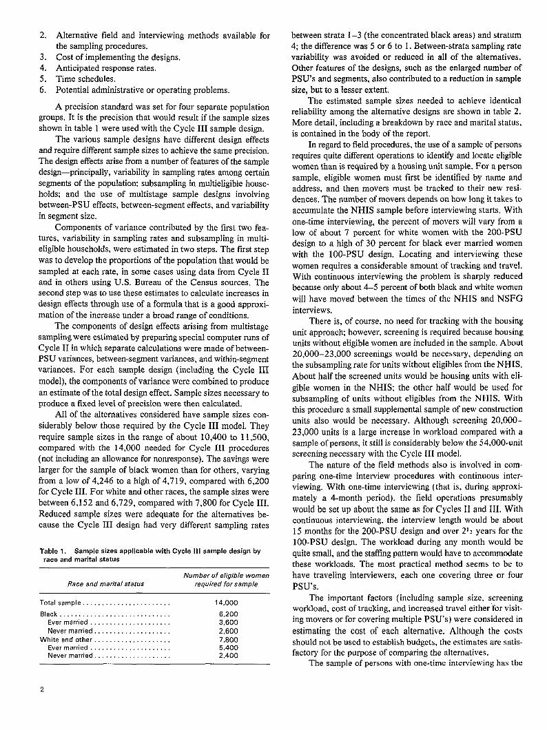
A precision standard was set for four separate populationgroups. It is the precision that would result if the sample sizesshown in table I were used with the Cycle III sample design.

The various sample designs have different design effectsand require different sample sizes to achieve the same precision.The design effects arise from a number of features of the sampledesign-principally, variability in sampling rates among certain

segments of the population: subsampling in multieligible house-holds; and the use of multistage sample designs involvingbetween-PSU effects, between-segment effects, and variabilityin segment size.

Components of variance contributed by the first two fea-tures, variability in sampling rates and subsampling in multi-eligible households, were estimated in two steps. The first step

was to develop the proportions of the population that would be

sampled at each rate, in some cases using data from Cycle Hand in others using U.S. Bureau of the Census sources. Thesecond step was to use these estimates to calculate increases in

design effects through use of a formula that is a good approxi-mation of the increase under a broad range of conditions.

The components of design effects arising from multistagesampling were estimated by preparing special computer runs ofCycle II in which separate calculations were made of between-PSU variances, between-segment variances, and within-segmentvariances. For each sample design (including the Cycle III

model), the components of variance were combined to produce

an estimate of the total design effect. Sample sizes necessary toproduce a fixed level of precision were then calculated.

All of the alternatives considered have sample sizes con-siderably below those required by the Cycle III model. They

require sample sizes in the range of about 10,400 to 11,500,compared with the 14,000 needed for Cycle III procedures(not including an allowance for nonresponse). The savings were

larger for the sample of black women than for others, varyingfrom a low of 4,246 to a high of 4,719, compared with 6,200for Cycle III. For white and other races, the sample sizes were

between 6,152 and 6,729. compared with 7,800 for Cycle III.

Reduced sample sizes were adequate for the alternatives be-cause the Cycle III design had very different sampling rates

Table 1. Sample sizes applicable with Cycle III sample design byrace and marital status

Number of eligible women

Race and marital status raquired for sample

between strata 1–3 (the concentrated black areas) and stratum4: the difference was 5 or 6 to 1. Between-strata sampling ratevariability was avoided or reduced in all of the alternatives.Other features of the designs, such as the enlarged number ofPSU’S and segments, also contributed to a reduction in sample

size, but to a lesser extent.The estimated sample sizes needed to achieve identical

reliability among the alternative designs are shown in table 2.

More detail, including a breakdown by race and marital status,is contained in the body of the report.

In regard to field procedures, the use of a sample of personsrequires quite different operations to identify and locate eligiblewomen than is required by a housing unit sample. For a person

sample, eligible women must first be identified by name andaddress, and then movers must be tracked to their new resi-dences. The number of movers depends on how long it takes to

accumulate the NHIS sample before interviewing starts. With

one-time interviewing, the percent of movers will vary from alow of about 7 percent for white women with the 200-PSUdesign to a high of 30 percent for black ever married womenwith the 100-PSU design. Locating and interviewing these

women requires a considerable amount of tracking and travel.With continuous interviewing the problem is sharply reducedbecause only about 4–5 percent of both black and white women

will have moved between the times of the NHIS and NSFG

interviews.There is, of course, no need for tracking with the housing

unit approach; however. screening is required because housingunits without eligible women are included in the sample. About20,000–23,000 screenings would be necessary. depending onthe subsampling rate for units without eligibles from the NH IS.

About half the screened units would be housing units with eli-

gible women in the NHIS; the other half would be used forsubsampling of units without eligibles from the NHIS. Withthis procedure a small supplemental sample of new constructionunits also would be necessary. Although screening 20,000-

23,000 units is a large increase in workload compared with asample of persons, it still is considerably below the 54,000-unitscreening necessary with the Cycle HI model.

The nature of the field methods also is involved in com-

paring one-time interview procedures with continuous inter-viewing. With one-time interviewing (that is, during approxi-

mately a 4-month period), the field operations presumably

would be setup about the same as for Cycles 11 and HI. Withcontinuous interviewing, the interview length would be about15 months for the 200-PSU design and over 21z years for the1OO-PSU design. The workload during any month would be

quite small, and the stafYiig pattern would have to accommodatethese workloads. The most practical method seems to be to

have traveling interviewers, each one covering three or four

Psu’s.

Total sample . . . . . . . . . . . . . . . . . . . . . . .The important factors (including sample size. screening14,000

Black . . . . . . . . . . . . . . . . . . . . . . . . . . . . . 6,200workload, cost of tracking, and increased travel either ‘for visit-

Ever married . . . . . . . . . . . . . . . . . . . . . 3,600 ing movers or for covering multiple PSU’S ) were considered in

Never married . . . . . . . . . . . . . . . . . . . 2,600 estimating the cost of each alternative. Although the costsWhite and other . . . . . . . . . . . . . . . . . . . . 7,800

Ever married . . . . . . . . . . . . . . . . . . . . . 5,400should not be used to establish budgets, the estimates are satis-

Never married . . . . . . . . . . . . . . . . . . . . 2,400 factory for the purpose of comparing the alternatives.The sample of persons with one-time interviewing has the

.L

Table 2. Principal features of alternative sample and survey procedures

Approximate ApproximateSample Households Direct response

Design No.

interview

size screened cost rate periods

Number Percent

l........................................ 10,981

2 . . . . . . . . . . . . . . . . . . . . . . . . . . . . . . . . . . . . . . . . 10,398

3 . . . . . . . . . . . . . . . . . . . . . . . . . . . . . . . . . . . . . . . . 10,9814, . . . . . . . . . . . . . . . . . . . . . . . . . . . . . . . . . . . . . . . 10,3986 . . . . . . . . . . . . . . . . . . . . . . . . . . . . . . . . . . . . . . . . 10,6236 . . . . . . . . . . . . . . . . . . . . . . . . . . . . . . . . . . . . . . . . 11,023

7 . . . . . . . . . . . . . . . . . . . . . . . . . . . . . . . . . . . . . . . . 11,4488.. . . . . . . . . . . . . . . . . . . . . . . . . . . . . . . . . . . . . . . 14,000

10,981

10,39810,981

10,39823,11321,01720,42354,000

1,700,0001,870,000

2,630,000

2,610,0002,020,0002,020.0002,040,0002,610,000

81 Oct. 1987-Feb. 198882 Apr.-July 1986

83 Apr. 1985-Dee. 1987

83 Apr. 1985-June 198684 Ju[Y–Nov. 1986

84 Aug.-Dee. 198684 Sept. 1986-Jan. 198784 . . .

lowest cost. Estimates of the direct cost for this procedure areabout $1,700,000 for a 1OO-PSU design and close to $1,900,000for a 200-PSU sample. The cost for the sample of housingunits is fairly close, costing about $2,000,000. Continuous

interviewing costs much more, about $2,600,000, approxi-

mately the same as the Cycle III model.Response rates can be approximated only roughly. Some

of the reasons for this are a lack of experience with eligible

women who have previously been interviewed in NHIS, un-

known problems in tracking, the difilculty of following movers,and uncertainty about the public mood in regard to cooperationin surveys, However, approximations can be made of differ-

ences in response rate among the alternatives, and these dif-ferences are relevant for purposes of comparison.

Assuming that participation in the NHIS does not affect

cooperation, it is likely that the housing unit sample procedureswould have about the same nonresponse rates as the Cycle IIImodel. This applies if screening is carried out in a personalvisit immediately followed by the detailed interview, as was

done in Cycles 11and III. (If a different plan is followed, forexample, telephone screening, the nonresponse rate would in-crease, probably by 1-3 percent. ) The person samples wouldhave somewhat higher nonresponse rates than the housing unit

samples because of problems in tracking and in applying normal

conversion procedures to movers. Rough estimates of the in-creases in nonresponse rates over the Cycle III rate are asfollows: about 0.5 percent increase for continuous interviewing,1-112 percent for one-time interviewing with 200 PSU’S, and2-3 percent for one-time interviewing with 100 PSU’S.

The various alternatives have important implications for

the Cycle IV time schedule. The redesigned NHIS is not ex-

pected to start until January 1985. With the exception of con-tinuous interviewing. fieldwork cannot begin until the entiresample has been accumulated. This time period is needed to

create the sample of black eligible women, and it ranges fromabout 15 months for the 200-PSU person sample to 33 monthsfor the 100-PSU design. Thus, for one-time interviewing, theearliest interviewing starting dates are April 1986 for the 200-

PSU design and October 1987 for the 1OO-PSU design. Thehousing unit samples (in 200 PSU’S) could begin in July–September 1986. The continuous interview alternatives could

begin much earlier, probably about April 1985, because theyonly need pm-t of the sample to get started. It is possible to

be~in a little later because a modified continuous operation can

be envisioned in which interviewing starts later, near the end of1985 or early 1986, and catches up over the next few months.However, regardless of the starting dates, the earliest surveycompletion for continuous interviewing is June 1986 for the

200-PSU design and December 1987 for the 1OO-PSU sample.The earliest ending dates for the one-time interviewing areroughly the latter half of 1986 for the 200-PSU procedures andthe end of 1987 or early 1988 for the 100-PSU designs. Be-

cause the time period is so long with continuous interviewing,the possibilities of changing patterns of behavior exist andshould be taken into account in deciding among alternatives.

Operational and definitional concerns that result from usingthe NHIS as a sampling frame are discussed in the body of thereport. No major problems appear to exist that make any of the

alternatives clearly unacceptable. Each of the alternatives hassome advantages and disadvantages reflected in the estimated

costs, response rates, or time schedules.Two issues of particular note were identified. The first

relates to the geographic coverage of NHIS and NSFG. The

NHIS covers all 50 States and the District of Columbia, in-

cluding Hawaii and Alaska, whereas until now the NSFG hasexcluded Hawaii and Alaska. This does not pose any seriousproblem for Cycle IV because the Alaska and Hawaii data can

simply be excluded, and the remaining areas will be a prob-

ability sample of the 48 States. Some small amount of specialweighting may be necessary, but this is the only complication.

Alternatively, this may be an appropriate time to reconsiderwhether it is still advisable to exclude Hawaii and Alaska fromthe NSFG frame. Although the unit costs in these States wouldbe higher, the total cost would be increased only slightly because

only a few PSU’S would be selected from these two States. The

availability of the NHIS sample data would simplify expandingNSFG to represent the population of all 50 States.

The second issue is the advisability of some pilot studiesto address particular aspects of the alternatives for which ex-

perience is lacking. Probably the most important subject forstudy is the effectiveness of dhTerent methods of tracking movers.A second subject is to ascertain whether the materials that the

U.S. Bureau of the Census plans to make available are ade-quate to locate the sample persons or housing units and, if not,what kinds of maps, lists, or other materials are needed. Finally,

it would be useful to explore the effect of the alternatives on

nonresponse rates and to find out which population groupsrequire more intensive work on refusal conversion.

3

Chapter 2Descriptionof TheNationalSurvey ofFamily Growth, Cycle III

Background

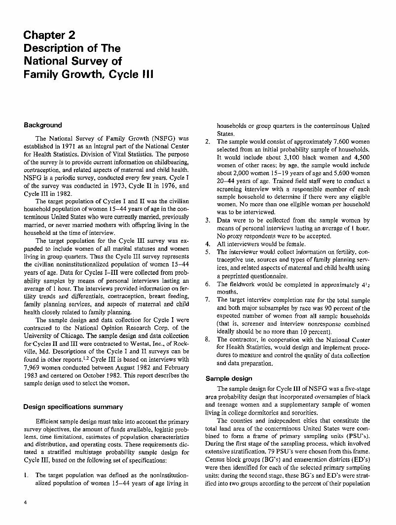
The Natiortal Survey of Family Growth (NSFG) was

established in 1971 as an integral part of the National Centerfor Health Statistics, Division of Vital Statistics. The purpose

of the survey is to provide current information on childbearing,contraception, and related aspects of maternal and child health.NSFG is a periodic survey, conducted every few years. Cycle I

of the survey was conducted in 1973, Cycle II in 1976, and

Cycle III in 1982.The target population of Cycles I and II was the civilian

household population of women 15–44 years of age in the con-terrninous United States who were currently married, previously

married, or never married mothers with offspring living in the

household at the time of interview.The target population for the Cycle 111 survey was ex-

panded to include women of all marital statuses and womenliving in group quarters. Thus the Cycle HI survey representsthe civilian noninstitutionalized population of women 15–44

years of age. Data for Cycles I-III were collected from prob

ability samples by means of personal interviews lasting anaverage of 1 hour. The interviews provided information on fer-tility trends and differentials, contraception, breast feeding,

family planning services, and aspects of maternal and child

health closely related to family planning.The sample design and data collection for Cycle I were

contracted to the National Opinion Research Corp. of. theUniversity of Chicago. The sample design and data collectionforCycles II and III were contracted to Westat, Inc., of Rock-ville, Md. Descriptions of the Cycle I and II surveys can be

found in other reports. 1.2Cycle III is based on interviews with

7,969 women conducted between August 1982 and February1983 and centered on October 1982. This report describes thesample design used to select the women.

Design specifications summary

Efficient sample design must take into account the primarysurvey objectives, the amount of funds available, logistic prob-lems, time limitations, estimates of population characteristicsand distribution, and operating costs. These requirements dic-tated a stratified multistage probability sample design for

Cycle III, based on the following set of specifications:

1.

4

The target population was defined as the noninstitution-

alized population of women 15–44 years of age living in

2.

3.

4.5.

6.

7.

8.

households or group quarters in the conterminous United

States.The sample would consist of approximately 7,600 womenselected from an initial probability sample of households.

It would include about 3,100 black women and 4,500women of other races: by age, the sample would include

about 2,000 women 15– 19 years of age and 5,600 women20–44 years of age. Trained field staff were to conduct a

screening interview with a responsible member of eachsample household to determine if there were any eligiblewomen. No more than one eligible woman per household

was to be interviewed.

Data were to be collected from the sample women bymeans of personal interviews lasting an average of 1 hour.No proxy respondents were to be accepted.

All interviewers would be female.The interviewer would collect information on fertility, con-traceptive use, sources and types of family planning serv-

ices, and related aspects of maternal and child health using

a preprinted questionnaire.The fieldwork would be completed in approximately 412months.The target interview completion rate for the total sample

and both major subsamples by race was 90 percent of theexpected number of women from all sample households

(that is, screener and interview nonresponse combinedideally should be no more than 10 percent).

The contractor, in cooperation with the National Centerfor Health Statistics, would design and implement proce-

dures to measure and control the quality of data collection

and data preparation.

Sample design

The sample design for Cycle III of NSFG was a five-stage

area probability design that incorporated oversamples of blackand teenage women and a supplementary sample of women

living in college dormitories and sororities.The counties and independent cities that constitute the

total land area of the conterminous United States were com-bined to form a frame of primary sampling units (PSU’S).During the first stage of the sampling process, which involvedextensive stratification, 79 PSU’S were chosen from this frame.

Census block groups (BG’s) and enumeration districts (ED’s)were then identified for each of the selected primary sampling

units; during the second stage, these BG’s and ED’s were strat-

ified into two groups according to the percent of their population

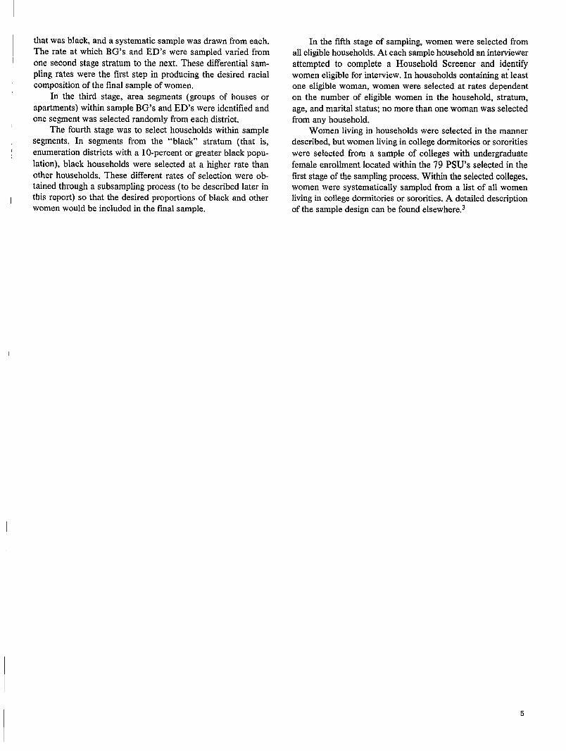
that was black, and a systematic sample was drawn from each.The rate at which BG’s and ED’s were sampled varied from

one second stage stratum to the next. These differential samp-ling rates were the first step in producing the desired racialcomposition of the final sample of women.

In the third stage, area segments (groups of houses or

apartments) within sample BG’s and ED’s were identified andone segment was selected randomly from each district.

The fourth stage was to select households within samplesegments. In segments from the “black” stratum (that is,

enumeration districts with a 10-percent or greater black popu-

lation), black households were selected at a higher rate than

other households. These different rates of selection were ob-tained through a subsampling process (to be described later inthis report) so that the desired proportions of black and otherwomen would be included in the final sample.

In the fifth stage of sampling, women were selected fromall eligible households. At each sample household an interviewer

attempted to complete a Household Screener and id:ntifywomen eligible for interview. In households containing at leastone eligible woman, women were selected at rates dependenton the number of eligible women in the household, stratum,

age, and marital status; no more than one woman was selectedfrom any household.

Women living in households were selected in the mannerdescribed, but women living in college dormitories or sororities

were selected from a sample of colleges with undergraduate

female enrollment located within the 79 PSU’S selected in thefirst stage of the sampling process. Within the selected colleges,women were systematically sampled from a list of all womenliving in college dormitories or sororities. A detailed descriptionof the smple design can be found elsewhere.3

5

Chapter 3Requirements of TheNational Survey ofFamily Growth, Cycle IV

It was assumed that Cycle IV was to consist of 14,000interviewed women, it was assumed that the distribution of thesample by race and marital status would be the same as theoriginal requirements for NSFG Cycle III, before the samplereduction and the oversarnpling of teenage women. This impliesthe sample distribution shown in table 1 in chapter 1. The re-quirements for sample size subsequently were modified so thatfor any sampling procedure being considered, the sample sizeshould produce the same sampling variances as would beachieved with the current design’s use of the sample sizes intable 1. Part of the present research is to ascertain these samplesizes.

Although most of the research is restricted to sample de-signs that have sampling errors consistent with table 1 samplesizes for the Cycle III sample design, it is prudent also to ex-plore at least one alternative sample size. For this alternative, asample size of 10,000 interviewed women with the same dis-tribution by race and marital status was chosen. First, it willgive some indication of the sensitivity of the sample design tothe sample size requirements. Second, it will provide the design

Table 3. Sample distribution for a raduced sample of10,000 women by race and marital status

Number of eligible women

Race and marital status required for sample

Total aample . . . . . . . . . . . . . . . . . . . . . . . 10,000

Black . . . . . . . . . . . . . . . . . . . . . . . . . . . . . 4,430Ever married . . . . . . . . . . . . . . . . . . . . . 2,570Naver married . . . . . . . . . . . . . . . . . . . . 1,860

White and other . . . . . . . . . . . . . . . . . . . . 5,570Ever married . . . . . . . . . . . . . . . . . . . . . 3,855Naver married . . . . . . . . . . . . . . . . . . . . 1,715

to be used in the event that there is a reduction in the fundsavailable for the survey. At this level the sample distribution isas shown in table 3. The implications of using this sample sizeare discussed in chapter 6. In addition to consideration of fea-sible sampling strategies, the cost and operational features ofvarious interviewing procedures have also been examined andare described in chapter 7.

6

Chapter 4Design effects in TheNational Survey ofFamily Growth withCycle III design

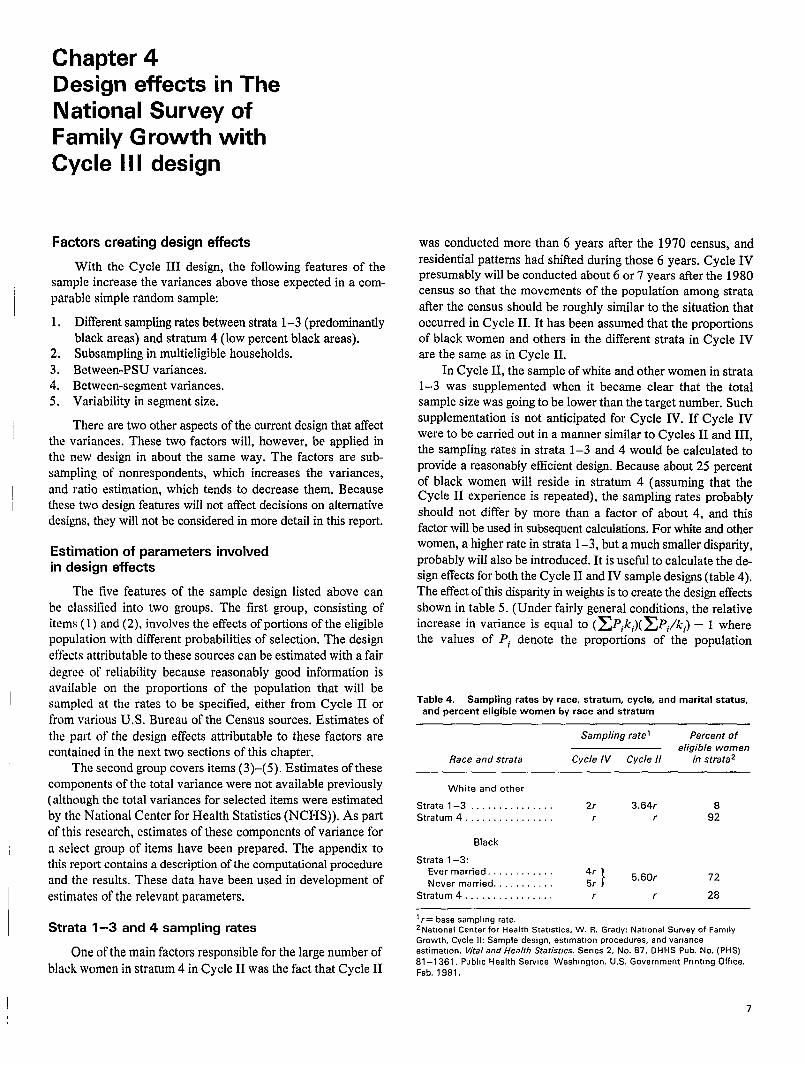
Factors creating design effects

With the Cycle III design, the following features of thesample increase the variances above those expected in a com-

parable simple random sample:

1, Different sampling rates between strata 1-3 (predominantlyblack areas) and stratum 4 (low percent black areas).

2, Subsampling in multieligible households.3, Between-PSU variances.

4. Between-segment variances.5, Variability in segment size.

There are two other aspects of the current design that affect

the variances. These two factors will, however, be applied inthe new design in about the same way. The factors are sub-sampling of nonrespondents, which increases the variances,

and ratio estimation, which tends to decrease them. Becausethese two design features will not affect decisions on alternativedesigns, they will not be considered in more detail in this report.

Estimation of parameters involvedin design effects

The tive features of the sample design listed above can

be classified into two groups. The first group, consisting ofitems ( 1) and (2), involves the effects of portions of the eligiblepopulation with different probabilities of selection. The design

effects attributable to these sources can be estimated with a fair

degree of reliability because reasonably good information isavailable on the proportions of the population that will besampled at the rates to be specified, either from Cycle II or

from various U.S. Bureau of the Census sources. Estimates of

the part of the design effects attributable to these factors arecontained in the next two sections of this chapter.

The second group covers items (3)–(5). Estimates of thesecomponents of the total variance were not available previously(although the total variances for selected items were estimated

by the National Center for Health Statistics (NCHS)). As partof this research, estimates of these components of variance for

a select group of items have been prepared. The appendix tothis report contains a description of the computational procedureand the results. These data have been used in development of

estimates of the relevant parameters.

Strata 1–3 and 4 sampling rates

One of the main factors responsible for the large number of

black women in stratum 4 in Cycle II was the fact that Cycle II

was conducted more than 6 years after the 1970 census, and

residential patterns had shifted during those 6 years. Cycle IVpresumably will be conducted about 6 or 7 years after the 1980census so that the movements of the population among strata

after the census should be roughly similar to the situation thatoccurred in Cycle II. It has been assumed that the proportionsof black women and others in the different strata in Cycle IVare the same as in Cycle II.

In Cycle II, the sample of white and other women in strata1–3 was supplemented when it became clear that the totalsample size was going to be lower than the target number. Suchsupplementation is not anticipated for Cycle IV. If Cycle IVwere to be carried out in a manner similar to Cycles II and III,the sampling rates in strata 1–3 and 4 would be calculated toprovide a reasonably eflicient design. Because about 25 percent

of black women will reside in stratum 4 (assuming that theCycle II experience is repeated), the sampling rates probably

should not differ by more than a factor of about 4, and thisfactor will be used in subsequent calculations. For white and otherwomen, a higher rate in strata 1–3, but a much smaller disparity,probably will also be introduced. It is useful to calculate the de-sign effects for both the Cycle 11and IV sample designs (table 4).The effect of this disparity in weights is to create the design effects

shown in table 5. (Under fairly general conditions, the relativeincrease in variance is equal to ( ~Piki)( ~i/ki) — 1 wherethe values of Pi denote the proportions of the population

Table 4. Sampling rates by race, stratum, cycle, and marital status,and percent eligible women by race and stratum

Sampling rate J Percent ofeligible women

Race and strata Cycle IV Cycle II in strata2

White and other

Strata l–3 . . . . . . . . . . . . . . . 2r 3.64r 8

Stratum 4 . . . . . . . . . . . . . . . . r r 92

81ack

Strata 1-3:Ever married . . . . . . . . . . . . 4r

Never married. . . . . . . . . . . 5r 15.60r 72

Stratum . . . . . . . . . . . . . . . . r r 28

1r= base sampllng rate.2Natlonal Center for Health Statistics, W. R. Grad~ Nat!onal Suway of Fam!ly

Growth, Cycle 11: Sample design, estimation procedures, and variance

estimation. Vita/ and Hea/th .9atistms. Series 2, No. 87. DHHS Pub. No. (PHS)81–1 361. Publm Health Service Washington. U.S. Government Pnntmg Office.Feb. 1981.

7

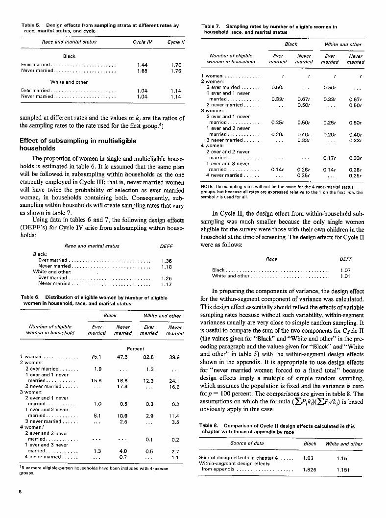
Table 5. Design effects from sampling strata at different rates byrace, marital status, and cycle

Table 7. Sampling rates by number of eligible women inhousehold, race, and marital status

Black White and other

Number of eligible Ever Never Ever Neverwomen in housahold married married married married

Race and marital status Cycle IV Cycle II

Black

Ever married . . . . . . . . . . . . . . . . . . . . . . . . 1.44 1.76Never married . . . . . . . . . . . . . . . . . . . . . . . 1.65 1.76

I woman . . . . . . . . . . . . .2 women:

2 ever married . . . . . . .1 ever and 1 never

married . . . . . . . . . . . .2 never married . . . . . .

3 women:2 ever and 1 never

married . . . . . . . . . . . .

1 ever and 2 nevermarried . . . . . . . . . . . .

3 never married . . . . . .4 women:

2 ever and 2 never

married . . . . . . . . . . . .1 ever and 3 never


r r r

0.50r

0.33r. . .

r

White and other

Ever married . . . . . . . . . . . . . . . . . . . . . . . . 1.04 1.14Never married . . . . . . . . . . . . . . . . . . . . . . . 1.04 1.14

0.50r

0.33r. . .

0.67r0.50r

0.67r0.50r

sampled at different rates and the values of ki are the ratios of

the sampling rates to the rate used for the first group.4)0.25r 0.50r 0.25r

0.20r. . .

0.50r

0.20r. .

0.40r0.33r

0.40r0.33rEffect of subsampling in mukieligible

households

The proportion of women in single and multieligible house-holds is estimated in table 6. It is assumed that the same planwill be followed in subsampling within households as the one

currently employed in Cycle III; that is, never married womenwill have twice the probability of selection as ever marriedwomen, in households containing both. Consequently, sub-sampling within households will create sampling rates that varyas shown in table 7.

Using data in tables 6 and 7, the following design effects(DEFF’s) for Cycle IV arise from subsampling within house-holds:

0.1 7r

0.14r. . .

0.33r. . . . . .

0.14r. .

0.28r0.25r

0.28r0.25r

NOTE The sampling rates will not be the same for the 4 race-marital status

groups. but because all rates are expressed relative to the 1 on the first line, the

avmbol r is used for all.

In Cycle II, the design effect from within-household sub

sampling was much smaller because the only single womeneligible for the survey were those with their own children in thehousehold at the time of screening. The design effects for Cycle IIwere as follows:Race and marital status DEFF

BlackEver married, . . . . . . . . . . . . . . . . . . . . . . . . . . . . . 1.36Never married . . . . . . . . . . . . . . . . . . . . . . . . . . . . . 1.IB

White and othecEver married . . . . . . . . . . . . . . . . . . . . . . . . . . . . . . 1.25Never married . . . . . . . . . . . . . . . . . . . . . . . . . . . . . 1.17

Race DEFF

Black . . . . . . . . . . . . . . . . . . . . . . . . . . . . . . . . . . . . . . 1.07

White and other . . . . . . . . . . . . . . . . . . . . . . . . . . . . . 1.01

In preparing the components of variance, the design effect

for the within-segment component of variance was calculated,

This design effect essentially should reflect the effects of variablesampling rates because without such variability, within-segmentvariances usually are very close to simple random sampling. It

is useful to compare the sum of the two components for Cycle II

(the values given for “Black” and “White and other” in the pre-

ceding paragraph and the values given for “Black” and” Whiteand other” in table 5) with the within-segment design effects

shown in the appendix. It is appropriate to use design effects

for “never married women forced to a fixed total” becausedesign effects imply a multiple of simple random sampling.which assumes the population is fixed and the variance is zeroforp = 100 percent. The comparisons are given in table 8. Theassumptions on which the formula ( ~iki)( ~i/ki) is basedobviously apply in this case.

Tabla 6. Distribution of eligibla women by number of eligiblawomen in household, race, and marital statua


Number of eligible Ever Never Ever Neverwomen in household married married married married

Percent

47.5 82.6I woman . . . . . . . . . . . . .

2 women:

2 ever married . . . . . . .1 ever and 1 never


3 women:2 ever and 1 never

married . . . . . . . . . . . .

1 ever and 2 never

married . . . . . . . . . . . .

3 never married . . . . . .4 women:l

2 ever and 2 nevermarried . . . . . . . . . . . .

1 ever and 3 never


75.1 39.9

1,9 . . . 1.3

15.6. . .

16.6 12.317.3 . . .

24.116.9

1.0 0.5 0.3 0.2

5.1. . .

10.9 2.92.5 .,.

11.43.5

Table 8. Comparison of Cycle II dasign effects calculated in thischapter with those of appendix by race

..- 0.1 0.2. . .Source of data Black White and other

1.3. . .

4.0 0.50.7 .,.

2.71.1 Sum of design effects in chapter 4 . . . . . . 1.B3 1.15

Within-segment design effectsfrom appendix . . . . . . . . . . . . . . . . .,, . . 1.825 1.15115 or more eligible-person households have been included with 4-person

groups.

8

Components of variance resulting frommultistage sampling

Consistency with NCHS calculations

Westat prepared estimates of the various components of

variance in Cycle II for use in estimating the intraclass corre-lations and other effects of multistage sampling. Before esti-mating these parameters, it is useful to compare the total design

effects of the calculations with those previously prepared byNCHS. Although NCHS reports did not explicitly reportdesign et~ects, it is easy to derive them from the data reported.

Design effects estimated b-vNCHS—In Vital and HealthSfa(isrics, Series 2, No. 87,2 page 23, NCHS indicates that anestimator for the relvariance under simple random sampling ofa proportion P’ for Cycle II is

where Z is the total population to which P’ applies, Q’ =1 – P’, and B takes the following values:

Race and marital status B

B1.+ckwomen ever marbled . . . . . . . . . . . . . . . . . . . 2,848.2

White and other women ever married. . . . . . . . . . 7,111.5

For the simple random sample, the relevant formula is. ofcourse.

where n is the sample size. The design effect DEFF is thus

DEFF = +

Values of Z, n, and DEFF from NSFG Cycle II are given intable 9.

Design effectsfrom JVestat computations—The design ef-fects shown in table 9 are applicable to percent distributions,

not to estimates of totals. The comparable Westat computations

are the ones in which the population totals were held fixed

because when this occurs, there is zero variance on estimatesof 100 percent of the population and the relvariances of esti-mates of totals and of associated percents are identical. For a

number of reasons, given in the appendix, the variances shown

are nut of the right dimensions and should not be used in com-

Table 9. NCHS computations of Cycle II values for Z’, n, and DEFFby race

Race z’ n DEFF

Blt?ck. . . . . . . . . . . . . . . . . . . . . . . . . 4,095,000 3,022 2.10White .+nd other . . . . . . . . . . . . . 25,647,000 5,589 1.55

SOURCE D N Krug, R. F. Slobasky, S. K, Hendncks. and J, Waksberg: Marmrra/

Survty of F,]mt/v GrowY/I Cyc/e // Final Repom. Contract No, HRA-1 06-74-153,

MW 1!377

parisons. However, the design effects and the proportions of

the variance attributable to the various stages of sampling arenot affected by the dimension and can be used. The designeffects shown in the tables of the appendix reflect only theeffect of within-segment sampling. The total design effect can

be obtained by dividing the within-segment design effect by theproportion of the variance arising from sampling households.The computations and comparisons with NCHS calculationsare shown in table 10. The estimates for white and other racesare a little further apart than expected. However, because ofthe rather small number of degrees of freedom used in both setsof computations, the difference probably is within sampling

error. The Westat computations, therefore, will be used to esti-mate intraclass correlations.

Between- PSU and between-segment variances

Some manipulation of the appendix data is necessary toproduce the PSU and segment intraclass correlations. The

equation

a~,=u2[l+a2+ b2+fip1+(; – l)p2+Vj

is a reasonable approximation of the total variance. P1 and p2

are the PSU and segment intraclass correlation coefllcients,

respectively, and ii and ; are the average number of sample

persons per sample PSU and sample segment, respectively.However, this formula assumes that all PSUS contribute to thebetween-PSU component of variance. Where there are self-representing PSU’S, the term Zpl should be replaced by l%P1,

where P is the proportion of the relevant population in non-self-

representing PSUS. In the expression for u?,, 1 + a2 + b2 =component from simple random sampling plus that from vari-ability in the sampling rate; Piip ~= effect of PSU samplingand (fi — 1)p2 -1-~ = effect of selecting segments: W. is theeffect of variability in segment size, and (Z – 1)p2 is the effect

of intraclass correlation within segments.The values shown in table 11 are developed from the ap

pendix. The values of P, Z and; come from the Cycle II sampledesign. They are shown in table 12 with the estimates of thedesired parameters. It has been estimated (somewhat arbitrarily)that J:= 0.0500.

Estimates of design effects for thecurrent 79- PSU design

Assuming

DEFF= 1 +PEpl +(Z– l)p2+a2+b2

Table 10. Comparison of Westat and NCHS computations of DEFF

by race

WhiteSource of data Black and other

Westat computations:

Within-segment DEFF. . . . . . . . . 1.825 1.151

W[thln-segment component ofvariance as proportion of total 0.890 0.653

Estimated total DEAF . . . . . . . . . . . . . . . . . 2.05 1.76NCHS computations: estimated total DEFF. . 2.10 1.55

9

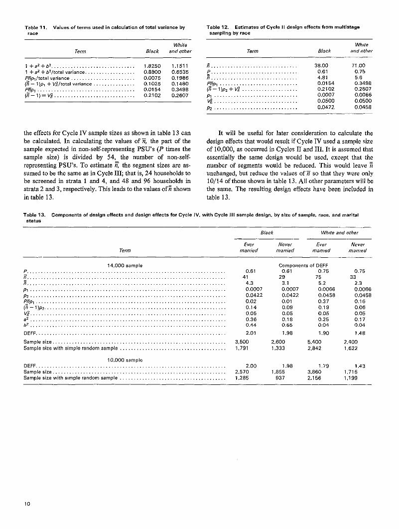
Table 11. Values of terms used in calculation of total variance byrace

Table 12. Estimates of Cycle I I design effects from multistagesampling by race

White

Term Black and other

l+a2+b2 . . . . . . . . . . . . . . . . . . . . . . . . . . . . . . 1,8250 1.1511l+a2+b2/total variance . . . . . . . . . . . . . . . . . . 0.8900 0.6535Pjpl/totalv ariance . . . . . . . . . . . . . . . . . . . . . . . 0.0075 0.1986(fi-l)pl +VF/total variance . . . . . . . . . . . . . . . 0.1025 0.1480Pulp, . . . . . . . . . . . . . . . . . . . . . . . . . . . . . . . . . . . 0.0154 0.3498(ii- l)= V; . . . . . . . . . . . . . . . . . . . . . . . . . . . . . 0.2102 0.2607

the effects for Cycle IV sample sizes as shown in table 13 canbe calculated. In calculating the values of Z, the part of thesample expected in non-self-representing PSU’S (P times thesample size) is divided by 54, the number of non-self-representing PSU’S. To estimate E the segment sizes are as-sumed to be the same as in Cycle III; that is, 24 households tobe screened in strata 1 and 4, and 48 and 96 households instrata 2 and 3, respectively. This leads to the values of Z shownin table 13.

White

Term Black and other

z.. . . . . . . . . . . . . . . . . . . . . . . . . . . . . .

PI . . . . . . . . . . . . . . . . . . . . . . . . . . . . . .

v . . . . . . . . . . . . . . . . . . . . . . . . . . . . . . .

Pa . . . . . . . . . . . . . . . . . . . . . . . .

38.00 71.000.61 0.754.81 5.60.0154 0.34980.2102 0.26070.0007 0.00660.0500 0.05000.0422 0.0458

It will be useful for later consideration to calculate thedesign effects that would result if Cycle IV used a sample sizeof 10,000, as occurred in Cycles II and III. It is assumed thatessentially the same design would be used, except that thenumber of segments would be reduced. This would leave ~unchanged, but reduce the values of Z so that they were only10/1 4 of those shown in table 13. All other parameters will bethe same. The resulting design effects have been included intable 13.

Table 13. Components of design effects and design effects for Cycle IV, with Cycle III sample design, by size of sample, race, and maritalstatus

Black Wh/te and other

Ever Never Ever NeverTerm married married married marrted

14,000 sampleP . . . . . . . . . . . . . . . . . . . . ...<... . . . . . . . . . . . . . . . . . . . . . . . . . . . . . . . . . . . . . . . . . . . .

Sample size . . . . . . . . . . . . . . . . . . . . . . . . . . . . . . . . . . . . . . . . . . . . . . . . . . . . . . . . . . . . . .

Sample size with simple random sample . . . . . . . . . . . . . . . . . . . . . . . . . . . . . . . . . . . . . .

10,000 sampleDEFF . . . . . . . . . . . . . . . . . . . . . . . . . . . . . . . . . . . . . . . . . . . . . . . . . . . . . . . . . . . . . . . . . . . .Sample size . . . . . . . . . . . . . . . . . . . . . . . . . . . . . . . . . . . . . . . . . . . . . . . . . . . . . . . . . . . . . .Sample size with s[mple random sample . . . . . . . . . . . . . . . . . . . . . . . . . . . . . . . . . . . . . .

0.6141

4.30.00070.04220.020.140.050.360.44

2.01

3,6001,791

2.002,5701,285

Components of DEFF0.61 0.75

29 753.1 5.20.0007 0.00660.0422 0.04580.01 0.370.09 0.19

0.05 0.050.18 0.250.65 0.04

1.98 1.90

2,600 5,400

1,333 2,842

1.98 1.791,855 3,860

937 2,156

0.7533

2.30.00660.04580.160.060.050.170.04

1.48

2,400

1,622

1,431,715

1,199

10

Chapter 5Design effects inalternative designs

Alternative designs considered

Six alternatives will be considered. Two will consist ofwhether to use all 200 PSU’S versus using 100 PSU’S. Twowill vary in whether the sample should consist of eligible womenin the NHIS (with movers being tracked) or whether the samplewill consist of sample addresses. In the latter case, both ad-dresses with and without eligibles will be included although theformer will be sampled at a much higher rate. (New constructionwill be treated as part of the noneligible addresses, ) Four of the

alternatives will be the four combinations of the two types ofplans. These four assume that data collection is performed in amoderately short time period, after the sample has been ac-

cumulated. The other two will consider the desirability of datacollection over a more lengthy period, in effect, following closelybehind the NHIS interviews. This method will be restricted toa sample of persons. When a sample of persons is used, there

will be very little difference in design effects and sample sizes

between the alternatives of continuous interviewing and carry-ing out the data collection in a limited period of time. Issuesrelating to the choice between these two will, therefore, be dis-

cussed in the section of this report on cost and operationalfeatures and not in the sample size sections.

In developing the properties of these designs, at least twoother parameters will be investigated. One is the period of time

to be used in the NHIS sampling frame. However, this will be

an output of the calculations. Once the desired sample sizes areknown, the minimum length of time for NHIS to supply thissize can be determined. This is the time period that should be

chosen. The other parameter is the subsampling rate to use innoneligible addresses, if that alternative is considered. This, inturn, will affect the NHIS period required. For the time being,the subsampling rate will be treated as a variable, to be deter-mined later.

Population projections for 1987

Table 14 has current data on marital status, by race, forwomen 15–44 and projections to 1987. The current figures, are

those for March 19815 (from P–20, No. 372). March 1981 isthe most recent U.S. Bureau of the Census report on marital

status. The projections for 1987 have been derived by usingU.S. Bureau of the Census projections for race and age6(P-25, No. 704) and assuming that the current proportions ofnever married women, by age, apply to 1987.

Table 15 summarizes the results, discounts the proportion

that will be lost because of the restriction that only one personper household can be interviewed, and contains estimates ofthe number of households that need to be screened to locate

one eligible woman.

Table 6 has been used to obtain the proportion of womenretained after loss due to multieligible households. The totalnumber of households in 1987 comes from the Series B pro-

jections in P–25, No. 805.7 Black households were estimatedas 12 percent of the total, a little higher than the 10.7 percentof the total reported by the U.S. Bureau of the Census in 1981s(see P-20, No. 371 ).

Table 14. Number of women 15-44 years, percent never married, and number never married, by age and race, 1981 and 1987 projections


1987 ?987 1981 1987

Never Never

Age Women Never married Women married Women Never married Women maried

Number inthousands

Total . . . . . . . . . . . . . . . . . . . . . . . . . 6,771

15-19 years . . . . . . . . . . . . . . . . . . . 1,460

20-24 years . . . . . . . . . . . . . . . . . . . 1,44525-29 years . . . . . . . . . . . . . . . . . . . 1,273

30-34 years . . . . . . . . . . . . . . . . . . . 1,075

35-39 years . . . . . . . . . . . . . . . . . . . 81940-44 years . . . . . . . . . . . . . . . . . . 699

Percent

48.0

96.4

68.835.7

20.713.8

8.6

Number In thousands

3,250 7,405 3,248 46,557

1,407 1,347 1,299 8,599

994 1,387 954 9,240454 1,390 496 8,705

222 1,313 272 8,150113 1,108 153 6,478

60 860 74 5,385

Percent

33.1

91.349.219.8

9.15.24.0

Number m thousands

15,415 48,625 14,114

7,849 7,425 6,7794,549 8,218 4,0431,725 9,020 1,786

738 8,820 803339 8,097 421215 7,045 282

11

Table 15. Eligible women, number of households, and households per eligible woman, by race and marital status, parcant eligible womenretained after loss in multieligible households, 1987 projections

Black Wh/te and other

Ever Never Ever NeverCharacteristic married married marr!ed married

Number In thousands

Eligible women . . . . . . . . . . . . . . . . . . . . . . . . . . . . . . . . . . . . . . . . . . . . . . . . . . . . . . . . . . . . . . . . . . 4,157 3,248 34,511 14,114Eligible women retained after loss in multieligible households. . . . . . . . . . . . . . . . . . . . . . . . . . . . 3,442 2,397 30,439 10,063Households . . . . . . . . . . . . . . . . . . . . . . . . . . . . . . . . . . . . . . . . . . . . . . . . . . . . . . . . . . . . . . . . . . . . . 11,021 80,820Households pereligible woman retainedl. . . . . . . . . . . . . . . . . . . . . . . . . . . . . . . . . . . . . . . . . . . . . 3.20 4.60 2.66 8.03

Percent

Eligibla women retained after loss in multieligible households. . . . . . . . . . . . . . . . . . . . . . . . . . . . 82.8 73.8 88.2 71.3

1Data do not include any allowance for nonreaponse or vacant housing units. Also, this screening ratio assumes the same subsampllng within households ss In Cycle III

For some alternates, It may be possible to reduce the amount of subsampllng.

Between- PSU variances

To estimate the between-PSU effect, it is necessary to

estimate ii and P for a 100- and a 200-PSU design. Some timeago Westat developed a 100-PSU design, and it is assumedthat the U.S. Bureau of the Census 1OO-PSU sample will be

generally comparable. This design was used to estimate P and

the number of non-self-representing PSU’S. Results also wereextrapolated to a 200-PSU design.

The values of the required parameters are in table 16.Strictly speaking, these values of Ptipl apply when a sample

size of 14,000 is used. Because some sample designs requiresmaller samples, from about 10,000 to 12,000 sample persons,the parameters will vary. However, because the difference issmall, and to simplifi the computations, the figures in table 16will be used for all alternatives.

Between-segment variances

For the Cycle III design, the segment sizes were 24 housingunits for strata 1 and 4, 48 for stratum 2, and 96 for stratum 3.However, the subsampling of white and other races was at such

a rate as to produce an effective segment size of 24 in strata 2

and 3, as well as in strata 1 and 4.

The NHIS segment sizes will be eight housing units if 1-year NHIS is used, 16 housing units if 2 years are used, and soforth. The values of (Z – 1)Pz are given in table 17.

Subsampling within households

In general, the same within-household subsampling pro-cedure will be applied as in the Cycle III design, and the valuesof b2 as shown in table 13 will apply to the various alternatives.For some alternatives it maybe possible to eliminate the within-

household subsampling for white and other races. In that case,this component of variance will be eliminated.

Differential sampling by strata

With the use of NHIS as a sampling frame, there will not

be any need to create the four strata used in the current design,

and the values of a2 used in table 13 will not apply. The sampledesigns being considered that involve following up persons whomove will not have any differential sampling rates. However,the alternative designs, which include all housing units that

have eligible women and a subsampling of the rest, will have

strata with different rates. For these alternatives, the additional

Table 16. Parameters for estimation of between-PSU effect by number of PSU’S, race, and marital status


Ever Never EverTerm

Nevermarried married married married

200 Psu’s

P . . . . . . . . . . . . . . . . . . . . . . . . . . . . . . . . . . . . . . . . . . . . . . . . . . . . . . . . . . . . . . . . . . 0.45 0.45 0.57 0.57Number ofnon-self-representing PSU’s. . . . . . . . . . . . . . . . . . . . . . . . . . . . . . . . . . . 110 110 110 110ii . . . . . . . . . . . . . . . . . . . . . . . . . . . . . . . . . . . . . . . . . . . . . . . . . . . . . . . . . . . . . . . . . . 15 11 28PI. . . . . . . . . . . . . . . . . . . . . . . . . . . . . . . . . . . . . . . . . . . . . . . . . . . . . . . . . . . . . . . . .

12

0.0007 0.0007 0.0066 0.0066Pip, . . . . . . . . . . . . . . . . . . . . . . . . . . . . . . . . . . . . . . . . . . . . . . . . . . . . . . . . . . . . . . . 0.01 0.01 0.11 0.05

100 Psu’s

P . . . . . . . . . . . . . . . . . . . . . . . . . . . . . . . . . . . . . . . . . . . . . . . . . . . . . . . . . . . . . . . . . . 0.50 0.50 0.62Number ofnon-self-representing PSU’s. . . . . . . . . . . . . . . . . . . . . . . . . . . . . . . . . . .

0.6266 66 66 66

ii . . . . . . . . . . . . . . . . . . . . . . . . . . . . . . . . . . . . . . . . . . . . . . . . . . . . . . . . . . . . . . . . . . 27 20 51 23PI. . . . . . . . . . . . . . . . . . . . . . . . . . . . . . . . . . . . . . . . . . . . . . . . . . . . . . . . . . . . . . . . . 0.0007 0.0007 0.0066 0.0066Pip,. . . . . . . . . . . . . . . . . . . . . . . . . . . . . . . . . . . . . . . . . . . . . . . . . . . . . . . . . . . . . . . 0.01 0.01 0.21 0.09

12

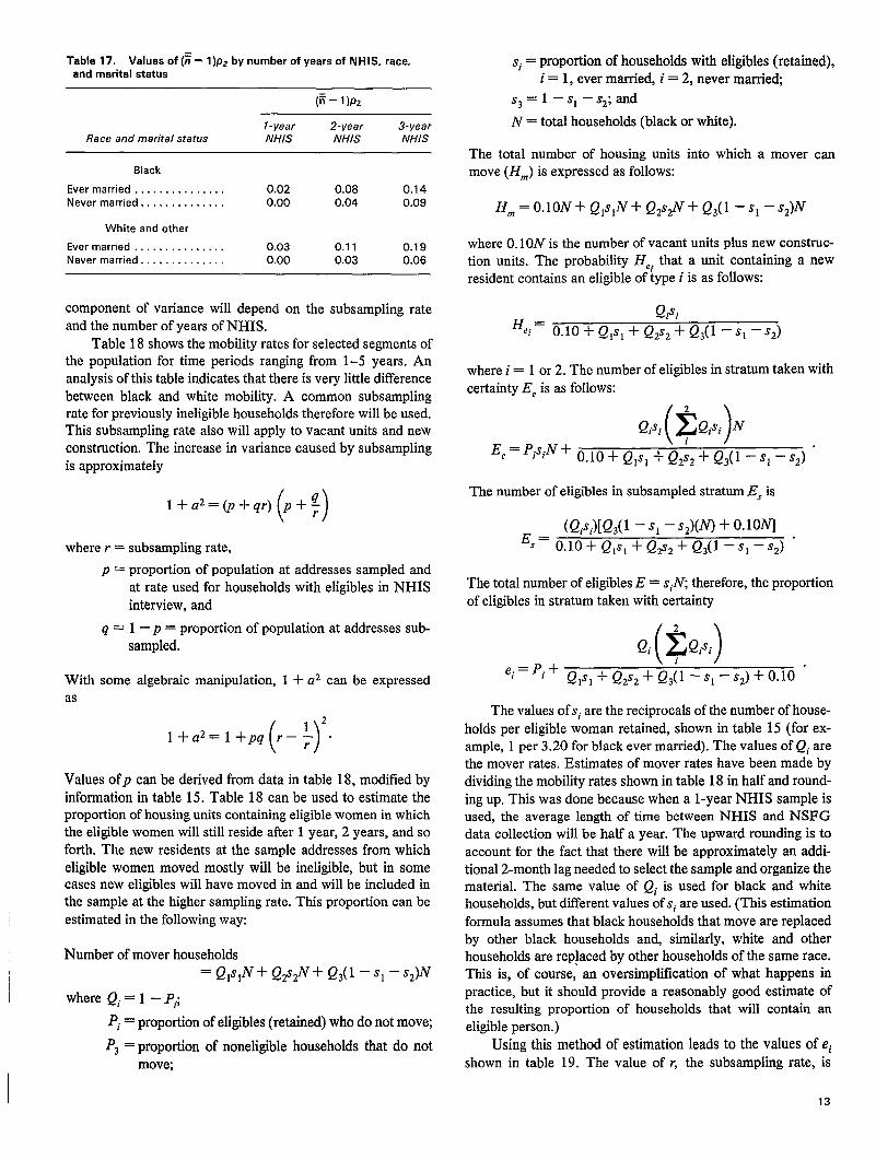
Table 17. Valuea of (; -1 )pz by number of years of NH IS, race,and maritel status

(ii– 1)pz

l-year 2-year 3-yearRace and marital status NH/S NHIS NHIS

Black

Ever married . . . . . . . . . . . . . . . 0.02 0.08 0.14Never married . . . . . . . . . . . . . . 0.00 0.04 0.09

White and other

Ever married . . . . . . . . . . . . . . . 0.03 0.11 0.19Never married...,.......,.. 0.00 0.03 0.06

component of variance will depend on the subsampling rateand the number of years of NHIS.

Table 18 shows the mobility rates for selected segments ofthe population for time periods ranging from 1-5 years. Ananalysis of this table indicates that there is very little differencebetween black and white mobility, A common subsarnplingrate for previously ineligible households therefore will be used.This subsampling rate also will apply to vacant units and newconstruction. The increase in variance caused by subsamplingis approximately

()l+a2=(p+qr) p+$

where r = subsampling rate,

p = proportion of population at addresses sampled andat rate used for households with eligibles in NHISinterview, and

4 = 1 – p = proportion of population at addresses sub-sampled.

With some algebraic manipulation, 1 + a2 can be expressedas

()2

l+a2=l+pq r–~ .

Values ofp can be derived from data in table 18, modified byinformation in table 15. Table 18 can be used to estimate theproportion of housing units containing eligible women in whichthe eligible women will still reside after 1 year, 2 years, and soforth. The new residents at the sample addresses from whicheligible women moved mostly will be ineligible, but in somecases new eligibles will have moved in and will be included inthe sample at the higher sampling rate. This proportion can beestimated in the following way

Number of mover households= Q,sIN+ Q2S2N+ Q3(1 –sl –S2)N

where Qi = 1 – P;

Pi= proportionof eligibles (retained) who do not move;

P3 = proportionof noneligible households that do notmove;

Si= proportion of households with eligibles (retained),i = 1, ever married, i =2, never marrie~

s3=l —sl —s2; and

N= total households (black or white).

The total number of housing units into which a mover canmove (HJ is expressed as follows:

Hm = O.1ON+ QISIN+ Q&N+ Q3(1 –sl ‘S2)~

where O.10N is the number of vacant units plus new construc-tion units. The probability H,i that a unit containing a newresident contains an eligible of type i is as follows:

Qisi

‘ej= O.1O+ QIS1+ Q2S2+ Q3(1 –S1 ‘S2)

where i = 1 or 2. The number of eligibles in stratum taken withcertainty ECis as follows:

Qisi(~Qisi)N/

‘c= ‘isiN+ O.1O + QIS1 + ~2;2 + Q3(1 – SI – ~2)

The number of eligibles in subsampled stratum E, is

(Qisi)[Q3(l – sl – S2)(N) + O.1ONI‘S= O.lO+QIS1 +Q~2+ Q3(1 –s, –s2) “

The total number of eligibles E = siN, therefore, the proportionof eligibles in stratum taken with certainty

L )Qi ~Qisi

‘i=pi+ Q,s, + Q2s2+ b3il ‘S1’-S2) +0.10 “

The values of si are the reciprocals of the number of house-holds per eligible woman retained, shown in table 15 (for ex-ample, 1 per 3.20 for black ever married). The values of Qi arethe mover rates. Estimates of mover rates have been made bydividing the mobility rates shown in table 18 in half and round-ing up. This was done because when a l-year NHIS sample isused, the average length of time between NHIS and NSFGdata collection will be half a year. The upward rounding is toaccount for the fact that there will be approximately an addi-tional 2-month lag needed to select the sample and organize thematerial. The same value of Qi is used for black and whitehouseholds, but different values ofsi are used. (This estimationformula assumes that black households that move are replacedby other black households and, similarly, white and otherhouseholds are replaced by other households of the same race.This is, of course, an oversimplification of what happens inpractice, but it should provide a reasonably good estimate ofthe resulting proportion of households that will contain aneligible person.)

Using this method of estimation leads to the values of eishown in table 19. The value of c the subsampling rate, is

13

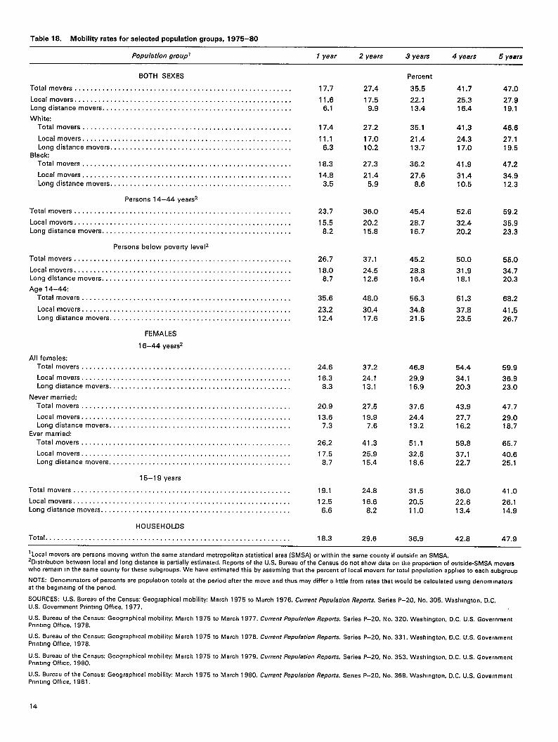
Table 18. Mobility ratea for aelectad population groupa, 1975-80

Population groupl 1 year 2 years 3 years 4 years 5 years

BOTH SEXES

Total movers .,, . .,, . . . . . . . . . . . . . . . . . . . . . . . . . . . . . . . . . . . . . . . . . . . . . . . .

Local movera . . . . . . . . . . . . . . . . . . . . . . . . . . . . . . . . . . . . . . . . . . . . . . . . . . . . . . .Long distance movers . . . . . . . . . . . . . . . . . . . . . . . . . . . . . . . . . . . . . . . . . . . . . . . .

White:Total movers . . . . . . . . . . . . . . . . . . . . . . . . . . . . . . . . . . . . . . . . . . . . . . . . . . . . .

Local movers . . . . . . . . . . . . . . . . . . . . . . . . . . . . . . . . . . . . . . . . . . . . . . . . . . . . .Long distance movers . . . . . . . . . . . . . . . . . . . . . . . . . . . . . . . . . . . . . . . . . . . . . .

BlackTotal movers . . . . . . . . . . . . . . . . . . . . . . . . . . . . . . . . . . . . . . . . . . . . . . . . . . . . .

Local movers, . . . . . . . . . . . . . . . . . . . . . . . . . . . . . . . . . . . . . . . . . . . . . . . . . . . .

Long distance movers...,,,..,.. . . . . . . . . . . . . . . . . . . . . . . . . . . . . . . . . . . .

Persons 14-44 yearsz

Total movers . . . . . . . . . . . . . . . . . . . . . . . . . . . . . . . . . . . . . . . . . . . . . . . . . . . . . . .

Local movera . . . . . . . . . . . . . . . . . . . . . . . . . . . . . . . . . . . . . . . . . . . . . . . . . . . . . . .

Long distance movers . . . . . . . . . . . . . . . . . . . . . . . . . . . . . . . . . . . . . . . . . . .,, ...

Persons below poverty Ievelz

Total movers . . . . . . . . . . . . . . . . . . . . . . . . . . . . . . . . . . . . . . . . . . . . . . . . . . . . . . .

Local movers . . . . . . . . . . . . . . . . . . . . . . . . . . . . . . . . . . . . . . . . . . . . . . . . . . . . . . .Long distance movers, . . . . . . . . . . . . . . . . . . . . . . . . . . . . . . . . . . . . . . . . . . . . . . .

Age 14-44:Totai movers . . . . . . . . . . . . . . . . . . . . . . . . . . . . . . . . . . . . . . . . . . . . . . . . . . . . .

Local movers . . . . . . . . . . . . . . . . . . . . . . . . . . . . . . . . . . . . . . . . . . . . . . . . . ,.. ,Long distance movers . . . . . . . . . . . . . . . . . . . . . . . . . . . . . . . . . . . . . . . . . . . . . .

FEMALES

16-44 yearsz

All females:Total movers . . . . . . . . . . . . . . . . . . . . . . . . . . . . . . . . . . . . . . . . . . . . . . . . . . . . .

Local movers . . . . . . . . . . . . . . . . . . . . . . . . . . . . . . . . . . . . . . . . . . . . . . . . . . . . .Long distance movers, . . . . . . . . . . . . . . . . . . . . . . . . . . . . . . . . . . . . . . . . . . . . .

Never married:Total movers . . . . . . . . . . . . . . . . . . . . . . . . . . . . . . . . . . . . . . . . . . . . . . . . . . . . .

Local movers.............,.. . . . . . . . . . . . . . . . . . . . . . . . . . . . . . . . . . . . . .Long distance movers . . . . . . . . . . . . . . . . . . . . . . . . . . . . . . . . . . . . . . . . . . . . . .

Ever married:Total movers, . . . . . . . . . . . . . . . . . . . . . . . . . . . . . . . . . . . . . . . . . . . . . . . . . . . .

Local movers.............,., . . . . . . . . . . . . . . . . . . . . . . . . . . . . . . . . . . . . .Long distance movers, . . . . . . . . . . . . . . . . . . . . . . . . . . . . . . . . . . . . . . . . . . . . .

15-19 years

Total movers . . . . . . . . . . . . . . . . . . . . . . . . . . . . . . . . . . . . . . . . . . . . . . . . . . . . . . .

Local movers,.,,..,..,,.,.,.. . . . . . . . . . . . . . . . . . . . . . . . . . . . . . . . . . . . . . .

Long distance molars . . . . . . . . . . . . . . . . . . . . . . . . . . . . . . . . . . . . . . . . . . . . . . . .

HOUSEHOLDS

Total . . . . . . . . . . . . . . . . . . . . . . . . . . . . . . . . . . . . . . . . . . . . . . . . . . . . . . . . . . . . . .

17.7

11.66.1

17.4

11.16.3

18.3

14.8

3.5

23.7

15.58.2

26,7

18,08.7

35.6

23.212.4

24.6

16.38.3

20.9

13.67.3

26.2

17.58.7

19.1

12.5

6.6

18.3

27.4

17.59.9

27.2

17.010.2

27.3

21.4

5.9

36.0

20.2

15.8

37.1

24.512.6

48.0

30.417.6

37.2

24.113.1

27.5

19.97.6

41.3

25.915.4

24.8

16.6

8.2

29.6

Percant

35.5

22.113.4

35.1

21.413.7

36.2

27.6

8.6

45.4

28.716.7

45.2

28.816.4

56.3

34.821.6

46.8

29,916.9

37.6

24.413.2

51.1

32.518,6

31.5

20.511.0

36.9

41.7

25.316.4

41.3

24.317.0

41.9

31.4

10.5

52.6

32.420.2

60.0

31.918.1

61,3

37.823.5

54.4

34.120.3

43.9

27.716.2

59.8

37.122.7

36.0

22.613.4

42.8

47.0

27,919.1

46.6

27.119.6

47,2

34.912.3

59.2

35.9

23.3

55.0

34.720.3

68.2

41.526.7

59.9

36.923.0

47.7

29,018.7

66.7

40.625.1

41,0

26.114.9

47.9

‘Locsl movers srepersonsmovmg wlth!nthe same standard metropolitan statistical area (SMSA) orwithin thasame county ifoutaidasn SMSA.‘Dlstnbutton between local and Iongdtstance is partially estimated. Reports of the U.S. Bureau of the Census donot show data ontha proportion of outside-SMSA moverswho remain In the same county forthesa subgroups. We hava estimated this by assuming that the percent of local movars for total population applies to each subgroup

NOTE: Denominators ofparcenta arepopulat!on totals attheperiod aftar the move andthus maydiffer almlefr omratesth atwould recalculated uslngdenomlnatora

at the beglnnmg of the period.

SOURCES: U. S. Bureau of the Census: Geographical mobility March 1975to March 1976. Current Population Repotis. Serias P-20, No.305. Washington, D.C.

U.S. Government Printing OffIce, 1977.

U.S. Bureau of the Census Geographical mobilitfi March 1975 to March 1977. Current Popu/atiorr Reports. Series P–20, No. 320. Washington, D.C. U.S. Government

Pr!ntlng Offtce, 1978.

U.S. Bureau of the Cenaus Geographical mobi[ity March 1975to March 1978. Current Population Reports. Seriea P-20, No. 331. Washington, D.C. U.S. Government

Printing OffIce, 1978.

U.S. Bureau of the Census Geographical mobillty March 1975 to March 1979. Current Population Reports. Series P–20, No. 353. Washington, D.C. U.S. Government

PnntlngOfhce, 1980.

U.S. Bureau of the Census: Geographical mobility March 1975 to March 1980. Currerrf Population Reports. Senea P-20, No. 368. Waahlngton, D.C. U.S. Government

Prlnt!ng Office, 1981,

14

Table 19. Design effect components arising from subsampling housing units without eligible women in NH IS by race and marital status


Ever Never Ineligible Ever Never Ineligible TotalTerm and NHIS time period married married [= 03] married married (= Q) households

s. . . . . . . . . . . . . . . . . . . . . . . . . . . . . . . . . . . . . . . . . . . . . . . . . . . .

Q,l-year NH IS . . . . . . . . . . . . . . . . . . . . . . . . . . . . . . . . . . . . . . . . . .2-year NHIS . . . . . . . . . . . . . . . . . . . . . . . . . . . . . . . . . . . . . . . . . .3-year NHIS . . . . . . . . . . . . . . . . . . . . . . . . . . . . . . . . . . . . . . . . . .

e,

l-year NH IS . . . . . . . . . . . . . . . . . . . . . . . . . . . . . . . . . . . . . . . . . .2-year NH IS, . . . . . . . . . . . . . . . . . . . . . . . . . . . . . . . . . . . . . . . . .3-year NHIS . . . . . . . . . . . . . . . . . . . . . . . . . . . . . . . . . . . . . . . . . .

a2

r = Y2:

l-year NH IS,,.,.,..,,,....,.,.. . . . . . . . . . . . . . . . . . . . .2.year NHIS . . . . . . . . . . . . . . . . . . . . . . . . . . . . . . . . . . . . . . . .3-year NH IS . . . . . . . . . . . . . . . . . . . . . . . . . . . . . . . . . . . . . . . .

).= 1,/3:

I -year NHIS . . . . . . . . . . . . . . . . . . . . . . . . . . . . . . . . . . . . . . . .Z-year NH IS . . . . . . . . . . . . . . . . . . . . . . . . . . . . . . . . . . . . . . . .3-year NH IS . . . . . . . . . . . . . . . . . . . . . . . . . . . . . . . . . . . . . . . .

r= !~:

l-year NHIS . . . . . . . . . . . . . . . . . . . . . . . . . . . . . . . . . . . . . . . .2-year NH IS . . . . . . . . . . . . . . . . . . . . . . . . . . . . . . . . . . . . . . . .3-yaar NHIS . . . . . . . . . . . . . . . . . . . . . . . . . . . . . . . . . . . . . . . .

1/3.20

0.15

0.220.26

0.950.920.91

0.020.040.04

0.060.100.11

0.110.170.18

1/4.60

0.12

0.15

0.20

0.96

0.940.93

0.02

0.030.03

0.050.080.09

0.09

0.130.15

1/2.13

0.07

0.13

0.14

. . .

. . .

. . .

. . .

,..

. . .

. . .

1/2.66

0.15

0.22

0.26

0.93

0.890.88

0.03

0.050.05

0.090.130.14

0.15

0.22

0.24

1/8.03

0.12

0.15

0.20

0.95

0.930.91

0.02

0.030.04

0.060.090.11

0.110.150.18

1/1.69 . . .

0.08 0.10

0.13 0.160.15 0.19

. . . . . .

. . .

. . . .

. . . . . .#.. . . .

. . .

. . . .,.

. . . . . ..

. .

. . . . . ..

()2

NOTE: a2 = e,(i - e,) ~ ;-&\r

Table 20. Total d,esign affects with alternative sample designs by race and marital status


Ever Never Ever NeverSample design married marria d married married

Current design . . . . . . . . .

Sample of persons withtrscking

200 Psu’s:l-year NH IS .,......,2-year NHIS. ,,, . . . . .3-year NH IS ..,..,.,.

100 Psu’s:l.year NHIS, . . . . . . . .2-year NH IS . . . . . . . . .3-year NHIS. ,., ,., . .

Sample of housing units,with subsampling

200 Psu’s:r = )5:

I -year NHIS .,.....2-yaar NHIS . . . . . . .3-year NH IS....,..

2.01 1.98 1.90 1.48

1.44 1.24 1.44 1.271.50 1.28 1.52 1.301.56 1.33 1.60 1.33

1.44 1.24 1.54 1.311.50 1.28 1.62 1.341.56 1,33 1.70 1.37

1.46 1.26 1.47 1.291.54 1.31 1.57 1.331.60 1.36 1.65 1.37

treated as an undetermined variable, r = ?4, ?4, and % are con-sidered as three potential values. Values of r less than % would

increase the variances to a level clearly inefficient.

Variability in segment size

Because NHIS will be based on area samples and will lagbehind the 1980 census for about the same amount of time as


Ever Never Ever Never

Sample design married married married married

f’= y3:

I -year NH IS....... 1.50Z-year NHIS . . . . . . . 1.603-year NH IS....... 1.69

r = 1/4:

l-year NH IS....... 1.552-year Nils . . . . . . . 1.673-year NHIS . . . . . . . 1.74

100 Psu’s:r = f/2:

l-year NH IS....... 1.46Z-year NH IS. . . . . . . 1.543-year NHIS. . . . . . . 1.60

r=E;l-year NH IS....... 1.502-year NHIS. . . . . . . 1.603-year NH IS. . . . . . . 1.69

r = 1/4;

l-year NH IS....... 1.552-year NH IS. . . . . . . 1.673-year NH IS. . . . . . . 1.74

1.25 1.53 1.331.36 1.65 1.391.29 1.74 1.44

1.33 1.58 1.381.41 1.74 1.451.48 1.84 1.51

1.26 1.57 1.331.31 1.67 1.371.36 1.75 1.41

1.29 1.63 1.371.36 1.75 1.431.42 1.84 1.48

1.33 1.68 1.421.41 1.84 1.491.48 1.94 1.55

the Cycle III design, the value of ~ should be the same as esti-mated earlier, that is, ~ = 0.05. -

Total design effect

The total design effect is one plus the various componentsdescribed above and shown in table 20. The design effectsfor the current sample design have been repeated in this table.

15

Chapter 6Sample sizes for alternativedesigns

Sample sizes needed for specifiedreliability

Denote the design effect for any statistic with the currentdesign as d and that for any particular alternative as d’. Let nbe the sample size with the current design and n’ for the alter-native. Then, if n’ is chosen to equalize the variances,

—=%dnz

n n’

andd’nt = —nd

Table 21 shows the sample sizes needed for each alternativeto produce equal variances.

Sample size available from NHIS for thealternative designs

For the alternatives comprising samples of women (ratherthan households), the sample sizes will be the number of house-holds available from NHIS divided by the number of house-holds per eligible retained, as shown in table 15. The number ofhouseholds to be visited is, of course, the same as the numberof women, because there will be one sample woman per house-hold. With a household sample, the household sample size willbe the number of households containing eligiblewomen in NHISplus the appropriate subsample of the remaining NHIS house-holds. These two components are shown separately in table21.The sample of women will consist of the number that would beavailable from a sample of women.

The first two lines of table 21 contain estimates of thenumber of sample black and whhe and other households thatwill be in NHIS annually after the NHIS redesign. The data onnumber of eligible women available for NSFG Cycle IV duringany specific period of time and the length of time necessary forNHIS to provide the samples required for each alternative arederived from these numbers. The assumptions used in makingthe

1.

2.

3.

16

household estimates are as follows:

The total number of interviewed households with viableaddresses in NHIS will be 50,000 per year.In the population as a whole, the proportion of black house-holds will increase from the 1981 level of about 11 to about12 percent in 1987, reflecting the increase in the blackpopulation.The NHIS revised sample will oversimple black house-holds by 20 percent. This will bring the percent of black

households in NHIS up to the level of a little over 14percent of all households.

4. Ten percent of NHIS interviews will be carried out bytelephone via random digit dialing and not be available forNSFG. It is assumed that the 10 percent loss will occurproportionally among black and white and other house-holds. The loss will actually be a little greater amongwhite households and a little less for black households be-cause of the lower telephone penetration in black house-holds, but this will probably approximately compensatefor some upward rounding in the estimated percent of blackhouseholds.

Three decisions are inherent in these assumptions—thetotal sample size, the 20-percent oversampling of black house-holds, and the 10-percent subsample to be carried out by randomdigit dialing. Any policy change on these three issues will changesome of the numbers. The only important item affected will belength of time necessmy for NHIS to supply the needed sample.None of the other conclusions in this report will be affected inany appreciable way.

Number of years of NHIS requiredto provide needed sample size

Comparing the sample sizes in table 22 with the numberavailable from NHIS in table 21 permits a calculation of theminimum number of years required for NHIS to provide theneeded sample. This, in turn, can be used to calculate the samplesizes. These data are shown in table 23, The minimum timeperiod in almost all cases includes fractional parts of years, andinterpolation methods are necessary for their estimation, be-cause tables 21 and 22 constitute full-year data. The followingalgorithms have been used for this estimation:

1. If the minimum period is less than 1 year, it is assumedthat the sample will consist of a subset of full segments. Forthe designs using a sample of persons, the design effectswill be the ones specified in table 20, and the fraction ofNHIS necessary to produce the required sample sizes forl-year NHIS will be used. For the designs with subsam-pling, the same procedure is used, although this probablywill produce somewhat smaller sampling errors than theones desired because the proportion of movers will be alittle lower than the ones estimated. There are only a fewinstances in which this is of any importance, and the dif-ferences probably are well within the margin of error of theestimated parameters.

Table 21. Sampla sizes required for equal reliability with alternative sample designs by race end marital statua


Ever Never Ever NeverSample design married married married married Total

Currrmt design . . . . . . . . . . . . . . . . . . . . . . . . . . . . . . . . . . . . . . . . . . . . . . . . . . .

Sample of persons with tracking

200 Psu’s:l.year NHIS. . . . . . . . . . . . . . . . . . . . . . . . . . . . . . . . . . . . . . . . . . . . . . . . . . .2-year NHIS . . . . . . . . . . . . . . . . . . . . . . . . . . . . . . . . . . . . . . . . . . . . . . . . . . .3-year NH IS . . . . . . . . . . . . . . . . . . . . . . . . . . . . . . . . . . . . . . . . . . . . . . . . . . .

100 Psu’s:I -year NH IS . . . . . . . . . . . . . . . . . . . . . . . . . . . . . . . . . . . . . . . . . . . . . . . . . . .2-year NHIS . . . . . . . . . . . . . . . . . . . . . . . . . . . . . . . . . . . . . . . . . . . . . . . . . . .3-yaar NH IS . . . . . . . . . . . . . . . . . . . . . . . . . . . . . . . . . . . . . . . . . . . . . . . . . . .

Sample of housing units with subsampling

200 Psu’s:~= yt:

l.year NHIS. ,, . . . . . . . . . . . . . . . . . . . . . . . . . . . . . . . . . . . . . . . . . . . . . .2.year NHIS . . . . . . . . . . . . . . . . . . . . . . . . . . . . . . . . . . . . . . . . . . . . . . . . .3-yaar NHIS . . . . . . . . . . . . . . . . . . . . . . . . . . . . . . . . . . . . . . . . . . . . . . . . .

r=%:l.year NHIS . . . . . . . . . . . . . . . . . . . . . . . . . . . . . . . . . . . . . . . . . . . . . . . . .2.year NHIS. . . . . . . . . . . . . . . . . . . . . . . . . . . . . . . . . . . . . . . . . . . . . . . . .3.year NH IS . . . . . . . . . . . . . . . . . . . . . . . . . . . . . . . . . . . . . . . . . . . . . . . . .

r = ~/4:

l-year NHIS, . . . . . . . . . . . . . . . . . . . . . . . . . . . . . . . . . . . . . . . . . . . . . . . .2-year NHIS . . . . . . . . . . . . . . . . . . . . . . . . . . . . . . . . . . . . . . . . . . . . . . . . .3.year NHIS . . . . . . . . . . . . . . . . . . . . . . . . . . . . . . . . . . . . . . . . . . . . . . . . .

100 Psu’s:r = ~%:

l-year NHIS. . . . . . . . . . . . . . . . . . . . . . . . . . . . . . . . . . . . . . . . . . . . . . . . .2-year NHIS. . . . . . . . . . . . . . . . . . . . . . . . . . . . . . . . . . . . . . . . . . . . . . . . .3-year NH IS . . . . . . . . . . . . . . . . . . . . . . . . . . . . . . . . . . . . . . . . . . . . . . . . .

/’ = y3:l-year NHIS, . . . . . . . . . . . . . . . . . . . . . . . . . . . . . . . . . . . . . . . . . . . . . . . .2-year NHIS. . . . . . . . . . . . . . . . . . . . . . . . . . . . . . . . . . . . . . . . . . . . . . . . .3-year NHIS . . . . . . . . . . . . . . . . . . . . . . . . . . . . . . . . . . . . . . . . . . . . . . . . .

r= {~:l-year NH IS . . . . . . . . . . . . . . . . . . . . . . . . . . . . . . . . . . . . . . . . . . . . . . . . .2-year NHIS. . . . . . . . . . . . . . . . . . . . . . . . . . . . . . . . . . . . . . . . . . . . . . . . .3-year NHIS . . . . . . . . . . . . . . . . . . . . . . . . . . . . . . . . . . . . . . . . . . . . . . . . .

3,600

2,5792,6872,794

2,5792,6872,794

2,6152,7582,866

2,6872,8663,027

2,7762,9913,116

2,6152,7582,866

2,6872,8663,027

2,7762,9913,116

2,600

1,6281,6811,746

1,6281,6811,746

1,6551,7201,786

1,6941,7861,865

1,7461,8521,943

1,6551,7201,786

1,6941,7861,865

1,7461,8521,943

5,400

4,0934,3204,547

4,3774,6044,832

4,1784,4624,689

4,3484,6894,945

4,4914,9455,229

4,4624,7464,974

4,6334,9745,229

4,7755,2295,514

2,400

2,0592,1082,157

2,1242,1732,222

2,0922,1572,222

2,1572,2542,335

2,2382,3512,449

2,1572,2222,286

2,2222,3192,400

2,3032,4162,514

14,000

10,35910,79611,244

10,70811,14511,594

10,54011.09711,563

10,88611,59512,172

11,25112,13912,737

10,88911,44611,912

11,23611,94512,521

11,60012,48813,087

2. If the minimum period is more than 1 year, linear inter-polation will be used in the last year to estimate the samplesize necessary for the fraction of the year required. For asample between 1 and 2 years, if

m, = sample size needed in 1 year

mz = sample size needed in 2 years

nl = l-year NHIS

?tZ= 2-year NHIS

f= fraction of the second year

nl +~(rzz —n,) = sample available in 1 -1-j_years

ml +f(m2– ml)= sample needed in 1 +f years

then

f= ~, – n~~~~, – n,)

The sample size is nl -l-f(nz – nl).

Obviously, the same algorithm applies for a sample between2 and 3 years, with m, and n, defined as the second-year re-quirement and NHIS availability, and mz and nz comparablefigures for the third year. The period is then 2 +J

An examination of table 23 reveals some of the majorfeatures of the alternative designs. For the alternatives requiringsamples of persons with tracking, less than l-year NHIS isneeded for almost all of the sample of white women. For thesamples of black women, about 1% years are needed for a200-PSU design, and 2%-3 years for a 1OO-PSU design. A1OO-PSU design will require about 6 percent more interviewsthan a 200-PSU design for the same reliability. For the alter-natives in which housing units (or addresses) are the sampleunits, if one considers 3 years as the maximum period of NHISthat is practical, then a 1OO-PSU design cannot be used. A200-PSU design will provide enough sample cases of both blackand white women. With a housing unit sample, the number ofinterview cases needed is increased over the number required ifa sample of persons is used, the increase ranging from 2-10percent, depending on the subsampling rate.

Because it is assumed that a 3-year span is the maximum

17

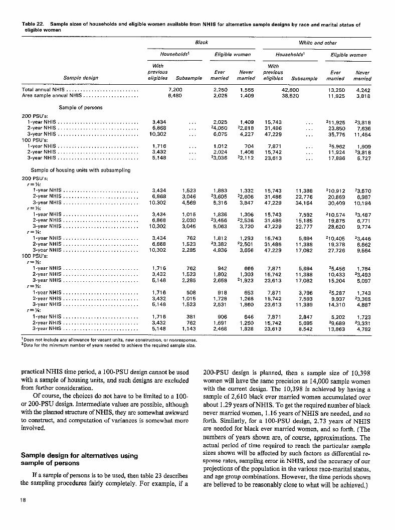
Table 22. Sample sizes of households and eligible women availabla from NHIS for alternative sample designs by race and marital status ofeligible women


Households Eligible women Households Eligible women

With Withprevious Ever Never previous Ever Never

Sample design eligibles Subsample married married eligibles Subsample married married

Total annua[NHIS . . . . . . . . . . . . . . . . . . . . . . . . . .Area sample annual NH IS . . . . . . . . . . . . . . . . . . . .

Sample of persons

200 Psu’s:I -year NH IS . . . . . . . . . . . . . . . . . . . . . . . . . . . . .2-year NHIS . . . . . . . . . . . . . . . . . . . . . . . . . . . . .

3-year NHIS . . . . . . . . . . . . . . . . . . . . . . . . . . . . .

100 PSU’a:I -year NH IS . . . . . . . . . . . . . . . . . . . . . . . . . . . . .2-year NHIS . . . . . . . . . . . . . . . . . . . . . . . . . . . . .3-year NH IS . . . . . . . . . . . . . . . . . . . . . . . . . . . . .


200 Psu’s:~ = y=:

I -year NHIS . . . . . . . . . . . . . . . . . . . . . . . . . . .2-yesr NHIS . . . . . . . . . . . . . . . . . . . . . . . . . . .

3-year NHIS . . . . . . . . . . . . . . . . . . . . . . . . . . .r = ~?:

l-year NH IS . . . . . . . . . . . . . . . . . . . . ... ,.. .2-year NH IS . . . . . . . . . . . . . . . . . . . . . . . . . . .3-year NHIS . . . . . . . . . . . . . . . . . . . . . . . . . . .

r = 7/4:

I -year NH IS..............,..,.. . . . . . . .2-year NHIS . . . . . . . . . . . . . . . . . . . . . . . . . . .3-year NHiS . . . . . . . . . . . . . . . . . . . . . . . . . . .

100 Psu’s:r = ~/2:

I -year NH IS . . . . . . . . . . . . . . . . . . . . . . . . . . .2-year NHIS . . . . . . . . . . . . . . . . . . . . . . ,, ...3-year NHIS . . . . . . . . . . . . . . . . . . . . . . . . . . .

r = ~%:I -year NHIS . . . . . . . . . . . . . . . . . . . . . . . . . . .2-year NHIS . . . . . . . . . . . . . . . . . . . . . . . . . .3-year NH IS . . . . . . . . . . . . . . . . . . . . . . . . . . .

r = ~/,:

I -year NHIS . . . . . . . . . . . . . . . . . . . . . . . . . . .2-year NHIS, . . . . . . . . . . . . . . . . . . . . . . . . . .3-year NHIS . . . . . . . . . . . . . . . . . . . . . . . . . . .

7,2006,480

2,2502,025

2,02524,050

6,075

1,0122,024

23,036

1,88323,605

5,316

1,83623,456

5,063

1,81223,3824,936

9421,8022,658

9181,7282,531

9061,6912,468

1,5651,409

1,40922,818

4,227

7041,408

22,112

1,33222,6063,847

1,30622,5363,720

1,29322,501

3,656

6661,303

21,923

6531,2681,860

6461,2501,628

42,80038,520

13,25011,925

4,2423,818

3,4346,666

10,302

1,7163,4325,148

3,4346,866

10,302

3,4346,868

10,302

3,4346,868

10,302

1,7163,4325,148

1,7163,4325,148

1,7163,4325,148

15,74331,48647,229

7.87115,74223,613

15,743

31,48647,229

15,74331,48647,229

15,74331,48647,229

7,87115,74223,613

7,87115,74223,613

7,87115,74223,613

211,92523,85035,775

23,8187,636

11,454

. . .

. . .

. . .

. . .

. . .

. . .

1,523

3,0464,569

1,0152,0303,045

7621,5232,285

7621,5232,285

5081,0151,523

381762

1,143

. . .

. . .

. . .

25,96211,92417,886

1,90923,8185,727

. . .

. . .

. . .

11,38822,77634,164

210,91220,86930,409

23,5706,987

10,194

7,59215,18522,777

210,57419,87528,620

23,/$87

6,7719,774

210,40519,37827,726

5,69411,38817,082

23,4466,6629,564

5,69411,38817.082

25,45610,43315,204

1,78423,493

5,097

3,7967,593

11,389

25,287

9,93714,310

1,74323,3854,867

2,8475,6958,542

5,20229,68913,863

1,72323,3314,782

I Does not include any allowance for vacant units, new constructmn, or nonresponse.2Dsta for the minimum number of years naeded to achieve the required sample size.

practical NHIS time period, a 1OO-PSUdesign cannot be usedwith a sample of housing units, and such designs are excludedfrom further consideration.

Of course, the choices do not have to be limited to a 100-or 200-PSU design. Intermediate values are possible, althoughwith the planned structure of NHIS, they are somewhat awkwardto construct, and computation of variances is somewhat moreinvolved.

200-PSU design is planned, then a sample size of 10,398women will have the same precision as 14,000 sample womenwith the current design. The 10,398 is achieved by having asample of 2,610 black ever married women accumulated overabout 1.29 years of NHIS. To get the required number of blacknever married women, 1.16 years of NHIS are needed, and soforth. Similarly, for a 1OO-PSU design, 2.73 years of NHISare needed for black ever married women, and so forth. (Thenumbers of years shown are, of course, approximations. Theactual period of time required to reach the particular samplesizes shown will be affected by such factors as differential re-sponse rates, sampling error ii NHIS, and the accuracy of ourprojections of the population in the various race-marital status,and age group combinations. However, the time periods shownare believed to be reasonably close to what will be achieved,)

Sample design for alternatives usingsample of persons

If a sample of persons is to be used, then table 23 describesthe sampling procedures fairly completely. For example, if a

18

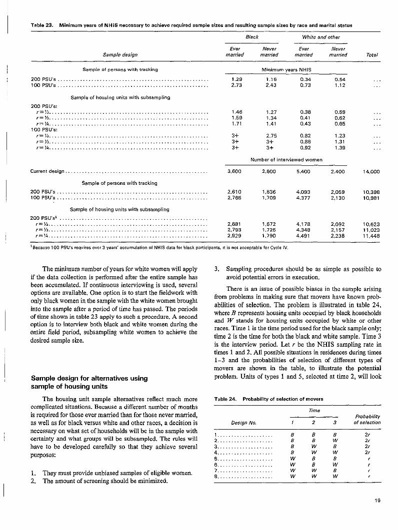
Table 23. Minimum years of NHIS necessery to achieve required sample sizes and resulting sample sizes by race and marital status


Ever Never Ever .NeverSample design married married married married Total


200 PSU’S. . . . . . . . . . . . . . . . . . . . . . . . . . . . . . . . . . . . . . . . . . . . . . . . . . . . . .100 PSU’S . . . . . . . . . . . . . . . . . . . . . . . . . . . . . . . . . . . . . . . . . . . . . . . . . . . . . .


200 Psu’s:r=y2...,,, . . . . . . . . . . . . . . . . . . . . . . . . . . . . . . . . . . . . . . . . . . . . . . . . . . .r= ~/3. . . . . . . . . . . . . . . . . . . . . . . . . . . . . . . . . . . . . . . . . . . . . . . . . . . . . . . . .~nl/ /4, ...,,..,.. . . . . . . . . . . . . . . . . . . . . . . . . . . . . . . . . . . . . . . . . . . . . . .

100 Psu’s:r=l,j..,.., .,, .

. . . . . . . . . . . . . . . . . . . . . .

r=% . . . . . . . . . . ..l. ..ll. ~.. ..; ;~; 1111111 . . . . . . . . . . . . . . . . . . . . . .r= ~.,....................,.. . . . . . . . . . . . . . . . . . . . . . . . . . . . . . . . .

Current design . . . . . . . . . . . . . . . . . . . . . . . . . . . . . . . . . . . . . . . . . . . . . . . . . . .


200 PSU’S . . . . . . . . . . . . . . . . . . . . . . . . . . . . . . . . . . . . . . . . . . . . . . . . . . . . . .100 PSU’S . . . . . . . . . . . . . . . . . . . . . . . . . . . . . . . . . . . . . . . . . . . . . . . . . . . . . .


200 PSU’S1 . . . . . . . . . . . . . . . . . . . . . . . . . . . . . . . . . . . . . . . . . . . . . . . . . . . . .r=y~. . .,, . . . . . . . . . . . . . . . . . . . . . . . . . . . . . . . . . . . . . . . . . . . . . . . . . . . .

r=%. . . . . . . . . . . . . . . . . . . . . . . . . . . . . . . . . . . . . . . . . . . . . . . . . . . . . . . . .~=:$ . . . . . . . . . . . . . . . . . . . . . . . . . . . . . . . . . . . . . . . . . . . . . . . . . . . . . . . . .

Minimum vears NHIS

1.29 1.16 0.34 0.542.73 2.43 0.73 1.12

1.46 1.27 0.38 0.591.59 1.34 0.41 0.621.71 1.41 0.43 0.65

3+ 2.75 0.82 1.233-1- 3+ 0.88 1.313+ 3+ 0.92 1.39

Number of interviewed women

3,600 2,600 5,400 2,400

2,610 1,636 4,093 2,0592,765 1,709 4,377 2,130

2,681 1,672 4,178 2,0922,793 1,725 4,348 2,1572,929 1,790 4,491 2,238

. . .

. . .

. . .

. . .

. . .

. . .

. . .

. . .

14,000

10,39810,981

10,62311,02311,448

1Because 100 PSU’S requires over 3 years’ accumulation of NHIS data for black participants, It is not acceptable for Cycle IV.

The minimum number of years for white women will applyif the data collection is performed after the entire sample hasbeen accumulated. If continuous interviewing is used, severaloptions are available. One option is to start the fieldwork withonly black women in the sample with the white women broughtinto the sample after a period of time has passed. The periodsof time shown in table 23 apply to such a procedure. A secondoption is to interview both black and white women during theentire field period, subsampling white women to achieve thedesired sample size.

Sample design for alternatives usingsample of housing units

The housing unit sample alternatives reflect much morecomplicated situations. Because a different number of monthsis required for those ever married than for those never married,as well as for black versus white and other races, a decision isnecessary on what set of households will be in the sample withcertainty and what groups will be subsampled. The rules willhave to be developed carefully so that they achieve severalpurposes:

1, They must provide unbiased samples of eligible women.2, The amount of screening should be minimized.

3. Sampling procedures should be as simple as possible toavoid potential errors in execution.

There is an issue of possible biases in the sample arisingfrom problems in making sure that movers have known probabilities of selection. The problem is illustrated in table 24,where B represents housing units occupied by black householdsand W stands for housing units occupied by white or otherraces. Time 1 is the time period used for the black sample only,time 2 is the time for both the black and white sample. Time 3is the interview period. Let r be the NHIS sampling rate intimes 1 and 2. All possible situations in residences during times1–3 and the probabilities of selection of different types ofmovers are shown in the table, to illustrate the potentialproblem. Units of types 1 and 5, selected at time 2, will look

Table 24. Probability of selection of movers

Time

Probability

Design No. 1 2 3 of selection

1.................... B B B 2r2. . . . . . . . . . . . . . . . . . . . B B w 2r

3 . . . . . . . . . . . . . . . . . . . . B w B 2r

4 . . . . . . . . . . . . B w w 2r

5:: : :: : : : . . . . . . . . . . . . w B B r

8 . . . . . . . . . . . . . . . . . . . . w B w r7 . . . . . . . . . . . . . . . . . . . . w w B r

8 . . . . . . . . . . . . . . . . . . . . w w w r

19

exactly the same at time 3. There is no way to distinguish them,but they have different probabilities of selection and should getdifferent weights. A similar situation exists for types 2 and 6,and soon. The problem for the white sample could be eliminatedby a change in the sampling rules. The new rule would excludeany white households selected at time 1 from the sample. Thiswould give all white households the same probability of selec-tion. However, we still would have the varying probabilitiesthat cannot be identified for black households.

To avoid this bias, it is necessary to use the same period oftime for both black and white households (and vacants and newconstruction). Subsampling of white households will be used toreduce the screening workload, but white households in bothperiods of time will need to be included.

Specific rules for subsampling are needed for implementingthis plan and coming as close as possible to the oversimplifiedversion of the sampling plan discussed earlier. Obviously, vari-ations in the rules can be made and, if the variations are not toogreat, the analyses and inferences probably are not greatly af-fected. Major variations are likely to affect the variances orcosts. One acceptable set of rules follows:

1. The time period to be used is the longest period needed forthe four race-marital status groups. In practice, this meansthe time period required for black ever married women.

2. Housing units in the NHIS sample containing black evermarried women will be included in NSFG with certainty.Housing units with exactly one white or other eligiblewomanwill be subsampied, the subsampling rate consisting of theratio of the time required for the particular group to thetime for the black ever married sample.

3. Housing units containing two or more black eligible womenwill be retained with certainty. Units with two or morewhite eligible units will be subsampled at the rates requiredto bring the rates for these women as close as possible tothe rates for women in white households with one eligiblewoman.

4. Vacant units and other addresses with no persons first will

be classified as in areas that are predominantly black orpredominantly white. They then will be subsampled at thesame rate as noneligible units of the same race.

5. New construction will be sampled at the same rate as vacantunits in white areas.

These rules deviate slightly from the assumptions made inestimating design effects and the resulting required sample sizes.For example, the design effects arising from subsampling withinmultieligible households will be reduced. Conversely, blackeligible women moving to new construction will be subsampledat a lower rate than shown in the assumptions. The overalleffect of the deviations seems to be fairly small and probably issmaller than errors in estimates of the parameters involved.Therefore, the sample sizes developed earlier will be used.

Screening workload with sample ofhousing units

Using information on the number of housing units in NHIS,the expected number with eligible women, and the samplingpatterns described in the previous section, the screening work-load can be estimated. A model of how this is done is shown intable 25.

Similar patterns can be developed for r = ?4and ?4and forthe 100-PSU designs. Table 26 summarizes the results. Forpurposes of comparability, data for the options using samplesof persons (rather than housing units) have also been included.For these alternatives, the number of households is identical tothe number to be interviewed. Table 26 contains a number ofassumptions, but they affect only a small part of the workload.The assumptions include that new construction will be at thelevel of 1.6 million units a year and that the number of vacantand converted units constitutes 10 percent of the total in bothblack and white areas (in addition to the assumptions aboutnumber of eligible women in the population and proportions ofmultieligible households previously discussed). The total work-load, including number of interviews and number of unitsscreened, is shown in table 27.

Table 25. Estimation of screening workloads for 200 PSU’S at r = Vz by race and type of housing unit

Annual Time Sub- NumberNHIS no. period Number sampling to be

Race and type of housing unit of units required in NHIS rate screened

Black housing units Years

I ever married . . . . . . . . . . . . . . . . . . . . . . . . . . . . . . . . . . . . . . . . . . . . . . 1,800 1.46 2,628 1.00 2,628Inevermarrled . . . . . . . . . . . . . . . . . . . . . . . . . . . . . . . . . . . . . . . . . . . . . 1,060 1.46 1,548 0.87 1,347Multiple eligibles . . . . . . . . . . . . . . . . . . . . . . . . . . . . . . . . . . . . . . . . . . . . 575 1.46 840 1.00 840No eligibles . . . . . . . . . . . . . . . . . . . . . . . . . . . . . . . . . . . . . . . . . . . . . . . . 3,045 1.46 4,446 0.50 2,223Vacant . . . . . . . . . . . . . . . . . . . . . . . . . . . . . . . . . . . . . . . . . . . . . . . . . . . . . 655 1.46 956 0.50 478

White and other housing units

I ever married . . . . . . . . . . . . . . . . . . . . . . . . . . . . . . . . . . . . . . . . . . . . . . 11,025 1.46 16,097 0.26 4,185l never married . . . . . . . . . . . . . . . . . . . . . . . . . . . . . . . . . . . . . . . . . . . . . 2,700 1.46 3,942 0.40 1,577Multiple eligibles . . . . . . . . . . . . . . . . . . . . . . . . . . . . . . . . . . . . . . . . . . . . 2,015 1.46 2,942 0.66 1,942No eligibles . . . . . . . . . . . . . . . . . . . . . . . . . . . . . . . . . . . . . . . . . . . . . . . . 22,780 1.46 33,259 0.20 6,652Vacant . . . . . . . . . . . . . . . . . . . . . . . . . . . . . . . . . . . . . . . . . . . . . . . . . . . . . 3,350 1.46 4,891 0.20New construction . . . . . . . . . . . . . . . . . . . . . . . . . . . . . . . . . . . . . . . . . . . .

978900 1.46 1,314 0.20 263

NOTE: The subsampl!ng rates for 1 ever married or 1 never married are the ratios of the minimum number of years for the groups in table 23 to the mmimum number of

years for black ever married The sampling rate for no eligibles and vacants is r times the rate for the larger of ever married or never married for the race, Vacants WIII be

classdied by the dominant race of the area In which they are located.

20

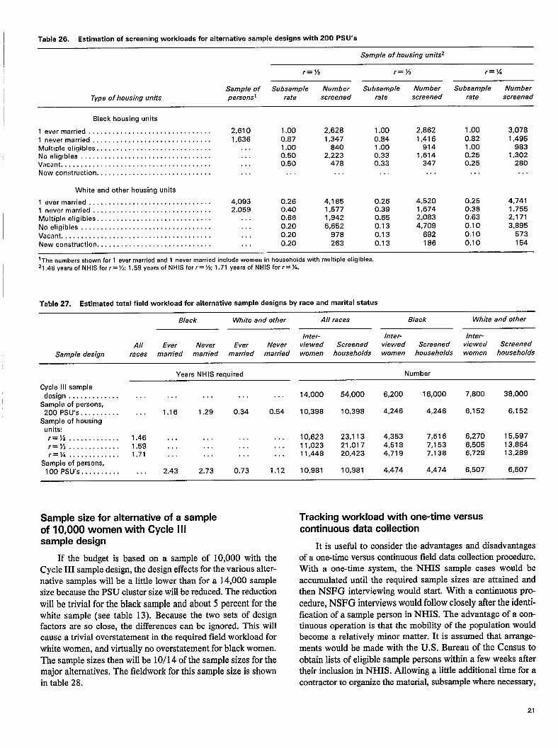
Table 26. Estimation of screening workloads for alternative aampIe designs with 200 PSU’S

Sample of housing units2

~=y= ~ = 1/3 j-= 1/4

Sample of Subsample Number Subsample Number Subsample Number

Type of housing units personsl rate screened rate screened rate screened

Black housing units

l ever married . . . . . . . . . . . . . . . . . . . . . . . . . . . . . . . 2,610 1.00 2,62B 1.00 2,862 1.00 3,078I never married . . . . . . . . . . . . . . . . . . . . . . . . . . . . . . 1,636 0.87 1,347 0.84 1,416 0.82 1,495Multlple eligibles . . . . . . . . . . . . . . . . . . . . . . . . . . . . . . . . 1.00 840 1.00 914 1.00 983Noeliglbles . . . . . . . . . . . . . . . . . . . . . . . . . . . . . . . . . . . . 0.50 2,223 0.33 1,614 0.25 1,302Vacant . . . . . . . . . . . . . . . . . . . . . . . . . . . . . . . . . . . . . . . . . 0.50 478 0.33 347 0.25 280New construction . . . . . . . . . . . . . . . . . . . . . . . . . . . . . . . . . . . . . . . . . . . . . . . . . .

White and other housing units

I ever married . . . . . . . . . . . . . . . . . . . . . . . . . . . . . . . 4,093 0.26 4,185 0.26 4,520 0.25 4,741I never married . . . . . . . . . . . . . . . . . . . . . . . . . . . . . . 2,059 0.40 1,577 0.39 1,674 0.38 1,755Multiple eligibles . . . . . . . . . . . . . . . . . . . . . . . . . . . . . . . . 0.66 1,942 0.65 2,083 0.63 2,171

No eligibles . . . . . . . . . . . . . . . . . . . . . . . . . . . . . . . . . . . . 0.20 6,652 0.13 4,709 0.10 3,895

Vacant . . . . . . . . . . . . . . . . . . . . . . . . . . . . . . . . . . . . . . . . . 0.20 978 0.13 692 0.10 573

New construction . . . . . . . . . . . . . . . . . . . . . . . . . . . . . . . . 0.20 263 0.13 186 0.10 154

‘The numbers shown for 1 ever married and 1 never married include women in households with multiple eligibles.21.46 yeara of NHIS forr=)!z: 1.59 years of NHIS forr=Ys; 1.71 years of NHIS forr= Y..

Teble 27. Estimated total field workloed for alternative sample designs by race and marital status

Black White and other All races Black White and other

hrter- hrter- lrrter-All Ever Never Ever Never vie wed Screened vie wed Screened vie wed

Sample design

Screened

races married married married married women households women households women households

Years NHIS required Number

Cycle Ill sampledesicm . . . . . . . . . . . . . . . . . . . . . . . . . . . . 14,000 54,000 6,200 16,000 7,800 38,000

SampIe of persons,200 PSU’S . . . . . . . . . . . . . 1.16 1.29 0.34 0.54 10,398 10,398 4,246 4,246 6,152 6,152

Sample of housingunits:r=l,’2 . . . . . . . . . . . . . 1.46 . . . . . . . . . 10,623 23,113 4,353 7,516 6,270 15,597r-!/-/3 . . . . . . . . . . . . . 1.59 . . . ::: . . . . . . 11,023 21,017 4,518 7,153 6,505 13,864r= ) %. . . . . . . . . . . . 1.71 . . . . . . . . . . . . 11,448 20,423 4,719 7,138 6,729 13,289

Semple of persona,100 PSU’S . . . . . . . . . . . . . 2.43 2.73 0.73 1.12 10,981 10,981 4,474 4,474 6,507 6,507

Sample size for alternative of a sample

of 10,000 women with Cycle IIIsample design

If the budget is based on a sample of 10,000 with theCycle III sample design, the design effects for the various alter-native samples will be a little lower than for a 14,000 samplesize because the PSU cluster size will be reduced. The reductionwill be trivial for the black sample and about 5 percent for thewhite sample (see table 13). Because the two sets of designfactors are so close, the differences can be ignored. This willcause a trivial overstatement in the required field workload forwhite women, and virtually no overstatement for black women.The sample sizes then will be 10/14 of the sample sizes for themajor alternatives, The fieldwork for this sample size is shownin table 28.

Tracking workload with one-time versuscontinuous data collection

It is usefhl to consider the advantages and disadvantagesof a one-time versus continuous field data collection procedure.With a one-time system, the NHIS sample cases would beaccumulated until the required sample sizes are attained andthen NSFG interviewing would start. With a continuous pro-cedure, NSFG interviews would follow closely after the identi-fication of a sample person in NHIS. The advantage of a con-tinuous operation is that the mobility of the population wouldbecome a relatively minor matter. It is assumed that arrange-ments would be made with the U.S. Bureau of the Census toobtain lists of eligible sample persons within a few weeks aftertheir inclusion in NHIS. Allowing a little additional time for acontractor to organize the material, subsample where necessary,

21

Table 28. Estimated total field workload for alternative sample designs with sample size of 10,000 by race and marital status

Black White and other All races Black White and other

hrter- /rrter- hrter-

All Ever Never Ever Never vie wed Screened vie wed Screened vie wed

Sample design races

Screened

married married marriad married women households women households women households

Years NHIS required Number

Cycle [11sampledesign . . . . . . . . . . . . . . . . . . . . . . . . . . . . 10,000 38,570 4,425 11,430 5,575 27,140

Sample of persons,

200 PSU’S . . . . . . . . . . . . . 0.83 0.92 0.24 0.39 7,427 7,427 3,033 3,033 4,394 4,394

Sample of housingunits:

/.= 1/2 . . . . . . . . . . . . . ... . . . . . . . . . . . . 7,588 16,510 3,109 5,369 4,479 11,141r= l/3...,,.,,..,.. . . . . . . . . . . . . . . . 7,873 15,012 3,227 5,109 4,646 9,903

r=qh . . . . . . . . . . . . . . . . . . . . . . . . . . . . 8,177 14,592 3,371 5,099 4,806 9,492

Semple of persons,100 PSU’S . . . . . . . . . . . . . 1.74 1.95 0.52 0.80 7,843 7,843 3,195 3,195 4,648 4,648

Table 29. Percent of movers in full sample of persons by distance of move, type of interviewing, race, and marital status

Total movers Local movers Long distance moversYearsNHIS l-time Continuous l-time Continuous l-time

No. of PSUS, race, and marital statusContinuous

required interviewing interviewing in tervie wing in tervie wing interwewii)g ir tervie wln’.q

200 Psu’s Percentl

Totalz. . . . . . . . . . . . . . . . . . . . . . . . . . . . . . . . . 11.0 4.8 7.3 3.2 3.7 1.6

Black:Ever mairied . . . . . . . . . . . . . . . . . . . . . . 1.16 17.6 5.2 11.7 3.5 5.9Never married.............,,. . . . . .

1.71.29 15.3 4.2 9.9 2.7 5.4

White and othec1.5

Ever married . . . . . . . . . . . . . . . . . . . . . . 0.34 6.8 5.2 4.6 3.5 2.2 1.7Never married . . . . . . . . . . . . . . . . . . . . . 0.54 7.5 4.2 4.9 2.7 2.6 1.5

100 PSU’a

Totalz . . . . . . . . . . . . . . . . . . . . . . . . . . . . . . . . . 18.8 4.9 12.4 3.2 6.4 1.7

BlackEver married . . . . . . . . . . . . . . . . . . . . . . 2.43 30.7 5.2 20.0 3.5 70.7Never married . . . . . . . . . . . . . . . . . . . . .

1.72.73 23.9 4.2 16.4 2.7 7.5

White snd othen

1.5

Ever married . . . . . . . . . . . . . . . . . . . . . . 0.73 11.8 5.2 7.9 3.5 3.9

Never married......,..,,.,.. . . . . . .

1.7

1.12 13.6 4.2 8.8 2.7 4.8 1.5

I For 1 -time intewiewing, we have assumed a 2-month lag in addition to the required number of years NH IS. The mobility rates then were those applmable to the

midpoint of the time interuel. For continuous interviewing, we heve assumed a 2-month lag and that the mobility rate is 20 percent of 1 -year mobility.

‘The total is the weighted average of the 4 subgroups, with the weights proportionate to the sample size.

and send the material to the interviewers, it is believed that the

NSFG interviews usually could be conducted about 2 monthsafter identification in NHIS. The proportion of movers then

would be quite low. As a result, there does not appear to be any

need for a housing unit sample with continuous interviewing.Analysis of continuous and one-time interviewing is, therefore,restricted to person samples.

Table 29 shows the percent of sample women who, at the

time of the NSFG interview, will no longer resi@e at the addressat which they were interviewed in NHIS. The table contains

data for the 200- and 1OO-PSUdesigns. Separate estimates areshown for local and long distance movers.

As can be seen, with 200 PSU’S and one-time interviewing,an estimated 11 percent of the sample women no longer will live

at their old addresses. Of this number, 3.7 percent will be long

distance movers and 7.3 percent local movers. The comparablefigures for continuous interviewing are 4.8, 1.6, and 3.2 percent,

With continuous interviewing, therefore, tracking is necessary

for less than half the number of cases required with a one-timedata collection period. The differences are even greater with a1OO-PSU sample design that will have about 18.8 percent

movers with one-time interviewing contrasted with 4.9 percent

with continuous data collection.The number of people who need to be followed will, of

course, affect the cost of the survey and probably the responserates. The costs of continu&s versus one-time interviewing

and management and administrative issues are discussed inchapter 7.

22

Chapter 7Costs, response rates, andtime schedule

costs the development of procedures and cost estimates for tracing

“movers,” rm effort that will be required if a decision is madeto use persons (that is, eligible respondents identified throughNHIS) as the sampling unit. Other possible concerns that couldbe examined in pilot studies are discussed in chapter 8. How-ever, no attempt was made as part of this report to estimate thecost of such an effort.

Computer costs have been included only for the manage-ment systems required to control a project of this magnitude

and complexity. It is assumed that the NCHS computer wouldbe used for data cleaning purposes.

All costs are estimated at first quarter 1983 price levels.

The reader should use his or her own judgment in estimatinghow various categories of cost might be expected to inflatebetween early 1983 and the actual period of contract per-formance.

Cost estimates (incorporating all the preceding caveats)are presented in summary form for eight possible designs intable 30. The sample sizes on which the costs are based arethose that will provide the same reliability (in terms of sampling

In this section cost estimates for the various possible de-signs for Cycle IV of NSFG are presented. All cost estimatesshown consist of direct costs only. Because the main purposeof the cost analysis was to arrive at relative costs of the variousdesigns, it was thought best to deal with estimates of direct costsonly. In this way, there was no need to speculate on the varia-tions in indirect cost structures among survey organizationsthat might perform the task of NSFG data collection. It maybenoted that indirect costs generally add another approximately50 pwcent to the direct costs for a survey of this size and com-

plexity,No pretest or pilot costs have been included in any of the

estimates. Regardless of the design chosen for Cycle IV, a

pretest primarily designed to test the questionnaire, the fieldprocedures, and the. data preparation procedures would be

conducted. There appears to be no reason to expect its cost tovary much among the several designs under consideration.

A pilot study might be in order, particularly with regard to

Table 30. Comparisons of direct costs, schedules, number of interviews, and response rates for alternative sample designs

Sample of persons Sample of housing units

1-time interviewing Continuous interviewing ~=y= ~= 1/3 ~=~~ Cycle Ill

100 Psu’smodel,

200 Pslrs 100 Psu’s 200 Psu’s 200 PslYs 80 PSIJ’S

Scheduling element Design 1 Design 2 Design 3 Design 4 Design 5 Design 6 Design 7 Design 8

Dollars

2,608,193 2,024,473

267,342 244,058145,182 173,948613,798 627,508

1,258,562 556,180

323,309 422,779

Total . . . . . . . . . . . . . . . . . . . . . . . . . 1,706,721

Professional labor. . . . . . . , . . . . . . . 249,134Clerical labor . . . . . . . . . . . . . . . . . . . 173,146Field labor . . . . . . . . . . . . . . . . . . . . . 519,205

Travel . . . . . . . . . . . . . . . . . . . . . . . . . 390,540

Ckher direct costs . . . . . . . . . . . . . . . 374,696

1,872,316

251,448156,762561,877540,965

361,264

2,632,006

285,470145,197615,359

1,252,687333.293

2,025,328

244,058176,707629,936556,180418,447

2,041,343

244,058179,488638.147556,180423,470

2,612,510

263,273211,201923,420468,995745,621

Months

27 18Schedule . . . . . . . . . . . . . . . . . . . . . . 18 18 45 18 18 20

Number

o 23,11310,398 10,623

Screening interviews . . . . . . . . . . . . 0Extended interviews. ., . . . . . . . . . . 10,981

010,398

010,981

21,01711,023

20,42311,448

54,00014,000

Rate

0.83 0.84Estimated responsel. . . . . . . . . . . . . 0.81 0.82 0.83 0.84 0.84 0.84

I Th~*w.tended mterwew response rate for Cycle Ill was 84.2 percentfor 20-44-year-old women and 83.8 percent for the total sampls, wh[ch included an oversamplinguf ttwnagers, ‘I’her@fore, 84 percent was used as the estimated response rate for Cycle IV, Design No. 8, All other response rates have been estimated reiatwe to the

CyclLI Ill model.

23

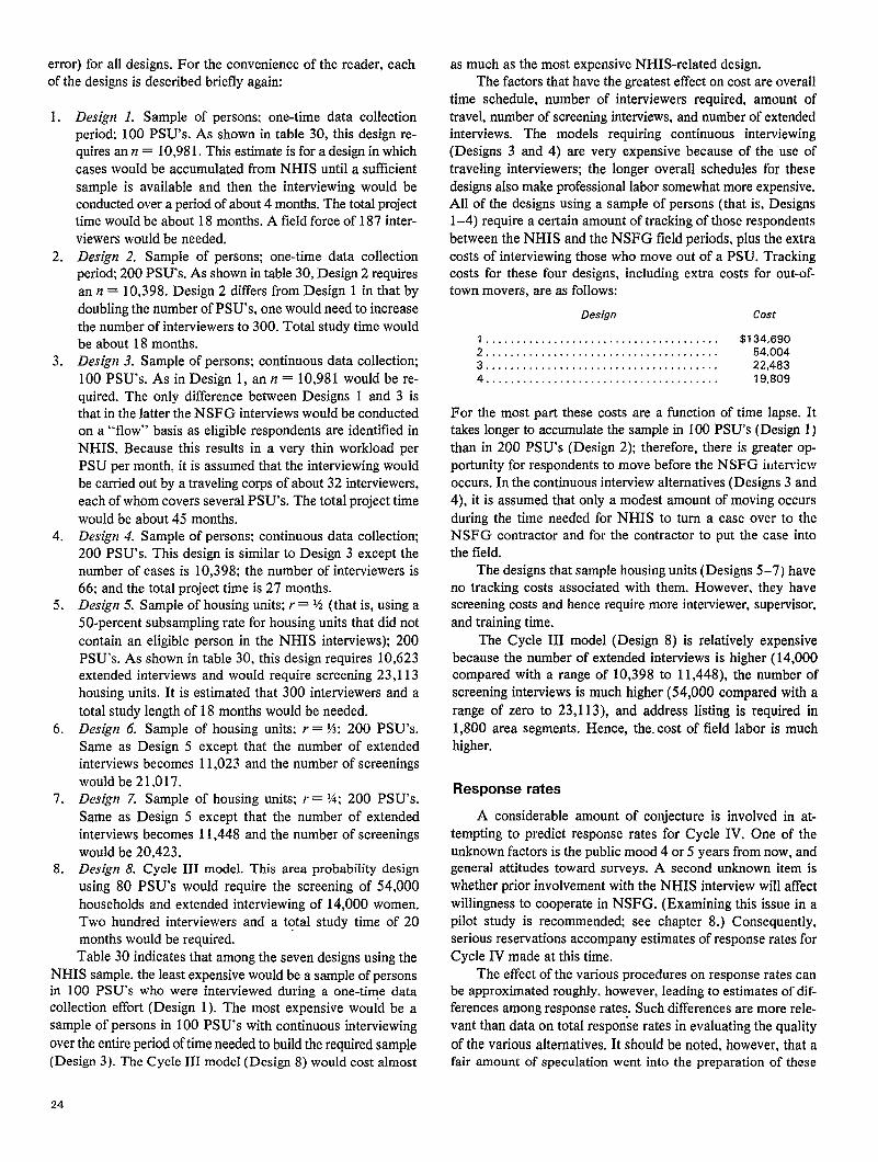
error) for all designs. For the convenience of the reader, eachof the designs is described briefly again:

1.

2.

3.

4.

5.

6.

7.

8.

Design 1. Sample of persons; one-time data collectionperiod: 100 PSU’S. As shown in table 30, this design re-quires an n = 10,981. This estimate is for a design in whichcases would be accumulated from NHIS until a sufficientsample is available and then the interviewing would beconducted over a period of about 4 months. The total projecttime would be about 18 months. A field force of 187 inter-viewers would be needed.Design 2. Sample of persons; one-time data collectionperiod 200 PSUS. As shown in table 30, Design 2 requiresan n = 10,398. Design 2 differs from Design 1 in that bydoubling the number of PSU’S, one would need to increasethe number of interviewers to 300. Total study time wouldbe about 18 months.Design 3. Sample of persons; continuous data collection;100 PSU’S. As in Design 1, an n = 10,981 would be re-quired. The only difference between Designs 1 and 3 isthat in the latter the NSFG interviews would be conductedon a “flow” basis as eligible respondents are identified inNHIS. Because this results in a very thin workload perPSU per month, it is assumed that the interviewing wouldbe carried out by a traveling corps of about 32 interviewers,each of whom covers several PSU’S. The total project timewould be about 45 months.Design 4. Sample of persons; continuous data collection;200 PSU’S. This design is similar to Design 3 except thenumber of cases is 10,398; the number of interviewers is66; and the total project time is 27 months.Design 5. Sample of housing units; r = % (that is, using a50-percent subsampling rate for housing units that did notcontain an eligible person in the NHIS interviews); 200PSU’S. As shown in table 30, this design requires 10,623extended interviews and would require screening 23,113housing units. It is estimated that 300 interviewers and atotal study length of 18 months would be needed.Des&n 6. Sample of housing units; r = M; 200 PSU’S.Same as Design 5 except that the number of extendedinterviews becomes 11,023 and the number of screeningswould be 21,017.Design 7. Sample of housing units; r = %; 200 PSU’S.Same as Design 5 except that the number of extendedinterviews becomes 11,448 and the number of screeningswould be 20,423.Design 8. Cycle III model. This area probability designusing 80 PSU’S would require the screening of 54,000households and extended interviewing of 14,000 women.Two hundred interviewers and a total study time of 20months would be required.Table 30 indicates that among the seven designs using the

NHIS sample, the least expensive would be a sample of personsin 100 PSU”S who were interviewed during a one-time datacollection effort (Design 1). The most expensive would be asample of persons in 100 PSU’S with continuous interviewingover the entire period of time needed to build the required sample(Design 3). The Cycle III model (Design 8) would cost almost

as much as the most expensive NHIS-related design.The factors that have the greatest effect on cost are overall

time schedule, number of interviewers required. amount oftravel, number of screening interviews, and number of extendedinterviews. The models requiring continuous interviewing(Designs 3 and 4) are very expensive because of the use oftraveling interviewers; the longer overall schedules for thesedesigns also make professional labor somewhat more expensive.All of the designs using a sample of persons (that is, Designs1–4) require a certain amount of tracking of those respondentsbetween the NHIS and the NSFG field periods, plus the extracosts of interviewing those who move out of a PSU. Trackingcosts for these four designs, including extra costs for out-of-town movers, are as follows:

Design cost

l . . . . . . . . . . . . . . . . . . . . . . . . . . . . . . . . . . . . . . $134,6902 . . . . . . . . . . . . . . . . . . . . . . . . . 54,0043: : : : : : : : : : : : : . . . . . . . . . . . . . . . . . . . . . . . . . 22,483

4 . . . . . . . . . . . . . . . . . . . . . . . . . . . . . . . . . . . . . . 19,809

For the most part these costs are a function of time lapse. Ittakes longer to accumulate the sample in 100 PSUS (Design 1)than in 200 PSUS (Design 2): therefore, there is greater opportunity for respondents to move before the NSFG ildmvicwoccurs. In the continuous interview alternatives (Designs 3 and4), it is assumed that only a modest amount of moving occursduring the time needed for NHIS to turn a case over to theNSFG contractor and for the contractor to put the case intothe field.

The designs that sample housing units (Designs 5-7 ) haveno tracking costs associated with them. However, they havescreening costs and hence require more interviewer, supervisor,and training time.

The Cycle III model (Design 8) is relatively expensivebecause the number of extended interviews is higher (14,000compared with a range of 10,398 to 11,448), the number ofscreening interviews is much higher (54,000 compared with arange of zero to 23,113), and address listing is required in1,800 area segments. Hence, the. cost of field labor is muchhigher.

Response rates

A considerable amount of conjecture is involved in at-tempting to predict response rates for Cycle IV. One of theunknown factors is the public mood 4 or 5 years from now, andgeneral attitudes toward surveys. A second unknown item iswhether prior involvement with the NHIS interview will affectwillingness to cooperate in NSFG. (Examining this issue in apilot study is recommended; see chapter 8.) Consequently,serious reservations accompany estimates of response rates forCycle IV made at this time.

The effect of the various procedures on response rates canbe approximated roughly, however, leading to estimates of dif-ferences among response rates. Such differences are more rele-vant than data on total respon~e rates in evaluating the qualityof the various alternatives. It should be noted, however, that afair amount of speculation went into the preparation of these

24

estimates, and they should be treated as indications of the order

of magnitude of differences in response rates.It is likely that the housing unit sample procedures (Designs

5-7) will have about the same nonresponse rates as theCycle III model (assuming that inclusion in NHIS has no effecton cooperation in NSF G). In interviewer-respondent interac-tions, Designs 5-8 are similar, consisting of a screening fol-lowed by the detailed interview. However, the same responserates would be expected for the four methods only if screening

is performed in a personal visit, to be followed immediately bythe detailed interview. If a different plan is followed for Designs

5-7 than for Design 8 (for example, telephone screening with a

followup in the form of a personal interview in eligible house-holds), the nonresponse rate is likely to increase. Experiencewith this kind of survey situation is limited but it is speculatedthat under these conditions response rates would decline by

1-3 percent.

It is likely that response rates for Designs 1–4 would be

somewhat below those for Designs 5-7. The need to trackmovers almost certainly will lower response rates. One reasonis that a few movers probably never will be located regardlessof the effort made in tracking. Second, some of the movers now

may reside in areas that are so far away from the sample PSU’S

that it is not practical to carry out the intensive conversionefforts normally applied.

The decline in response rates thus will depend partly on

the proportion of movers in the sample. As can be seen from

table 29, the expected percents of movers in Designs 1-4 are

Percent

18.811.0

4.94.8

Using these data, it is speculated that the decline in re-

sponse arising from tracking and followup of movers will beabout as follows:

1. Designs 3 and 4—an increase of perhaps 0.5 percent inthe nonresponse rate.

2. Design 2—an increase of about 1– 1.5 percent.3. Design 1—an increase of 2–3 percent.

Time schedule

There are two aspects of the Cycle IV time schedule thatshould be considered. One is the time period for essential survey

operations, for example, questionnaire development, training,

conduct of interview, data processing, and so forth. The otheris the time required to accumulate the necessary samplingmaterials in the NHIS and organize it for transmittal to theCycle IV survey operations group.

Table 30 contains, among other information, our estimatesof the time period needed for survey operations. As can beseen, all designs except those for continuous interviewing can

be completed in about the same period of time, 18 or 20 months.The Cycle III model takes a little longer than the others becauseof the additional time needed for sample selection, listing, andscreening. However, the difference between Cycle 111and De-

signs 1, 2, 5, 6, or 7 is quite small; also, these numbers shouldnot be taken too literally because at present only approximatetime schedules are possible.

Designs 3 and 4 will take much longer because of the nature

of the continuous intewiewing operation. The length of the actual

interviewing period will be about 4–6 months for all the non-continuous interview procedures. For continuous interviewing,it will be about 18 months for the 200-PSU design and 34

months for the 100-PSU design. The analytic implications ofthese increases in length of the interviewing period should betaken into account in choosing among the alternatives.

25

Chapter 8Other research issues

Scope and definitions in NH IS and NSFG

The definitions for the two surveys are essentially thesame. Both cover the civilian noninstitutionalized population,includingall eligiblepersons in ordinary housing units and board-ing houses; they exclude the institutionalized and military pop-ulation. The residence rules for college students are different inthe two surveys, but this does not afYectthe population covered.It simply means that college students selected in NHIS at onelocation may have to be interviewed in another.

There is one difference in the geographic coverage of thetwo surveys. NHIS covers all 50 States and the District ofColumbia, including Hawaii and Alaska, whereas NSFG hasexcluded Hawaii and Alaska. If NSFG is to retain the samegeographic coverage as in the past, it would not be complicatedor difticult to modify NHIS to exclude these two areas. In thecurrent NHIS design, Hawaii is a separate stratum. Eliminatingthe Hawaii PSU automatically will bring the estimates to the49-State level. Alaska has been combined with other north-western PSU’S. If the U.S. Bureau of the Census follows thesame policy in the redesigned NHIS, some reweighing of thesePSU’S will be needed. The adjustments will not be very large,and the effect should be trivial. This should not be an importantconsideration in deciding whether and how to use NHIS. Itshould be noted, however, that one or two NHIS PSU’S mayfall outside the sample. The 200-PSU sample thus may turnout to be about 198 PSU’S.

This may be an appropriate time for the National Centerfor Health Statistics to reconsider whether Hawaii and Alaskashould be excluded from the NSFG frame. There are someadvantages in having the survey cover all 50 States, and thusbe comparable with most demographic and social statisticsproduced by U.S. Government agencies. There is no intrinsicM13cultyin conducting interviews in PSU’S in these two States.The unit costs would be higher, stemming from such factors asincreased costs of bringing interviewers to central locations fortraining, higher recruiting costs, and higher costs for qualitycontrol and general communication. However, because it islikely that these costs will affect only one or two PSU’S, theeffect on the total budget will be fairly small. The availabilityof NHIS sample data would simplifi expanding NSFG to coverHawaii and Alaska.

In this report it has been assumed for cost and sample sizecalculations that all 50 States are to be covered. However, thishas only a minor effect on total costs and none of the conclu-sions would be changed if the survey were restricted to 48States, as in the past.

Staffing

If the data collection period is to be concentrated within afew months, starting after the entire NHIS sample has beenaccumulated, then the interview process will be quite similar tothe way Cycles II and III were carried out. In that case, using astaffing pattern similar to the one in Cycles II and III is sug-gested. This involves using local interviewers who are residentsof the sample PSU’S. The number of interviewers per PSU willdepend on the expected workload. The work assignments wouldbe made in more or less the same way as in Cycles 11and HI;that is, to minimize travel costs and, when feasible, to raciallymatch respondents to interviewers.

With continuous interviewing, the monthly workload perPSU will be quite small; therefore, traveling interviewers,somewhat in the manner used in the NHIS, are recommended.In general, one interviewer would be recruited to handle two tofour neighboring PSU’S, depending on the sample sizes anddistances between PSU’S.

Timing of NHIS and NSFG

No need for special action because of movement into andout of NHIS-screened housing units or into and out of agegroups is expected. Each of the alternatives discussed in thisreport has methods of handling persons who move that give alleligible persons known non-zero probabilities of selection. Asfar as age is concerned, the NHIS contains the ages of allsample persons by single years of age. Thus, it is possible tospecify the ages at time of NHIS interview that will make thedesignated women age eligible at the time of NSFG interview.

It is, of course, not possible to control marital status in thesame way as age. Some never married women will marry in theinterval between the NHIS and NSFG interviews. This doesnot cause any bias, but it does introduce a small amount ofuncertainty into the final sample sizes for ever married andnever married women. In addition, it implies that a small numberof ever married women will have been sampled as never marriedand carry their weights, and vice versa. Exact sample sizesnever have been possible in NSFG, and this is not a cause forconcern. In fact, for the alternative comprising samples of per-sons, use of NHIS should result in actual sample sizes beingmuch closer to the designated sample sizes than was possiblein the past.

Induction of sample persons

NHIS contains a considerable amount of information thatcould be used for stratification; for example, age of woman,

26

income, number of children living in household, and educa-tional attainment. Unfortunately, this information can be usedfor sample selection only to a limited degree. The ability tostratify depends on having a reasonably large pool of women

from which a sample is to be selected. Creating such a poolimplies using a long time period for NHIS during which the

sample is accumulated. For the alternatives considered, how-ever, long periods have deleterious effects. With samples ofpersons, a long period means that more persons have to betracked with attendant costs and potential increases in nonre-sponse rates. With samples of housing units, the effective strati-

fication of households into those containing eligibles and thosenot having eligibles will be weakened. The disadvantages arequite serious. In addition, the redesigned NHIS will only be inexistence a limited period of time when it will be necessary tostart NSFG, For these reasons, it is not practical to have a

long time period in NHIS from which to choose the NSFGsample. The following are suggestions for subsampling theNHIS file:

1.

2.

?. .

4,

There will be very little subsampling for black womew theNHIS time period used will be the minimum necessary tosupply the sample of black women. All black ever marriedwomen in NHIS in that period will be designated for NSFG

and about 90 percent of never married women. Stratificationcannot be applied effectively.With one-time interviewing of a sample of persons, it isrecommended that the sampled white women be thosemost recently in NHIS. Stratification cannot be used forwhite women with this alternative.

With continuous interviewing, a subsample of white women

will be selected for interviewing. At this time it is unclear

whether the sample will be drawn by the U, S. Bureau ofthe Census, in its field oftlces, or whether the U.S. Bureauof the Census will provide the entire list of eligible women

to a contractor who will select the sample. This is a detailthat will have to be worked out with the U.S. Bureau of theCensus,

If the U. S. Bureau of the Census selects the sample, itis recommended that no stratification be imposed. Withsuch decentralized sampling, it is more important to keepthe procedures simple than to attempt to squeeze the max-

imum efficiency out of the process. Possible errors resulting

from the added complexity of stratification could negateany statistical advantages. Items that appem to be effectivemodes of stratification can be introduced in the estimationprocedure in the form of poststratification. Their effective-

ness would be almost as great.

If a contractor carries out the sample selection, stratifi-

cation is feasible. It is recommended that items be usedthat seem to be important discriminators for fertility pat-terns, such as (a) for women 20 years of age and over,educational attainment and number of own children inhousehold; (b) for women under 20 years of age, school

enrollment and educational attainment of parents, How-ever, Cycle 111 data should be analyzed, when available,for a final decision on modes of stratification.

If Cycle IV consists of a sample of housing units, unitscontaining white eligible women also will be subsampled.

The policy recommended in paragraph(3) is again recom-mended.

In regard to the method of notfii~g sample persons thatthey are to be included in NSFG, the situation is somewhat

complicated. At the time of the NHIS interview, the U.S. Bureauof the Census interviewer will not know exactly who will be

included in NSFG (or other followup surveys). It is assumedthat the U.S. Bureau of the Census will wish to inform all re-spondents that they may be covered in other studies, withoutdescribing the other studies. In Cycles II and III, Westat sent a

letter to respondents prior to the interviewers’ visits. It is sug-

gested that this practice be continued. With a sample of per-sons, the letters could be addressed directly to the sample eli-gible women instead of “occupant” and thus be somewhat morepersonal.

In addition, it may be usefhl to have interim mailings if theprocedure to be used is a sample of persons with one-time in-terviewing. The purpose of the interim mailings would be toassist in tracking movers. The letters would ask potential re-spondents to notifi the National Center for Health Statistics orthe contractor of new addresses if they move betxveen the NHISand NSFG interview periods. Such actions seem to have helpedtracking in other studies. This may not be necessary or feasiblefor white respondents with a 200-PSU design. The time intervalbetween the two SUNeys willbe quite short and interim mailingsfor this group may be more of a nuisance than a help. It is more

useful with a 100-PSU sample and, of course, more importantfor the sample of black women than for white and other womenbecause of the much longer time period used for the accumula-tion of the sample of black women.

The continuation of the Cycle III practice of asking for

parental consent for teenagers at the time of the NSFG inter-viewers’ visits is suggested. The success rate in Cycle III wasquite good and no advantage could be anticipated by changing

the procedure.

Pilot studies

There are several issues that should be addressed in a pilotstudy, or possibly several small studies. (It may be uset%l todistinguish between the concept of pilot studies and the pretests

that have been conducted as part of Cycles II and III. Pretests

essentially are for the purpose of improving questionnaires,procedures, and training methods that have been decided upon.They act as “debugging” devices. Pilot studies are conductedat an earlier stage of preparation. They test whether some ap-

proaches are feasible and search for the best among several

alternatives. It is assumed that pretests will be carried out for

Cycle IV as in the past.)

It would be useful to study the methods of tracking movers.The possibility of interim mailings for access to more currentaddresses of the sample persons has been suggested. There are,of course, other methods that can be used to locate movers,

such as calling directory assistance, contacting the friends andrelatives supplied by the respondents in the NHIS interview,and writing to the sample persons and asking the post ot%ce toforward the mail. It is likely that all these methods will be used

to some extent, but it would be useful to get information on the

27

unit costs of these procedures and the success rate of each. Thiswould help in establishing an order of priority for the search

operation. It also would help in budgeting and in anticipating

nonresponse resulting from inability to locate some persons.

It also would be useful to investigate whether there areproblems in locating the sample addresses with the materials

supplied by the U.S. Bureau of the Census. There are severalkinds of materials the U.S. Bureau of the Census uses in thecourse of developing area samples: maps, listing forms, ad-

dresses of sample units, and names of residents, It is likely thattransmittal of street addresses and apartments is all that isneeded in most urban areas to locate the sample person, althoughthere may be some problems even in such areas in buildings

that do not have clearly identifiable apartment numbers. Goodstreet addresses do not exist in many rural areas. It would behelpful to ascertain whether information currently recorded bythe U.S. Bureau of the Census is sut%cient to locate virtually

all sample addresses, or if some modification of the U.S. Bureauof the Census forms is necessary.

A third item about which there is considerable uncertainty

is what effect the new procedures would have on nonresponserates. There is likely to be an increase in nonresponse caused

by a number of factors: Some movers may not be able to belocated in spite of intensive tracking efforts; a few may be lo-cated but are at such distances from sample PSU’S that it willnot be feasible to perform normal, intensive followup efforts;

and the fact that the respondents were subject to an earlierNHIS interview may influence their willingness to cooperate.It is doubtful that good estimates of rqsponse rates are possiblefrom a pilot study. (Pilot studies never seem to have the sample

sizes; the time that is necessary for a fi,dl, intensive followupeffom, the geographic distribution of the samplq or the com-mitment to carry out these operations as completely as neces-

sary.) However, it should be possible to get some indication ofthe increase in nonresponse rates, and for what populationgroups more intensive work on conversion is useful. At a min-imum, a pilot study on tracking should reveal how many cases

will involve intensive and/or expensive efforts to locate, and

what the increase in nonresponse would be if the efforts wererelaxed.

28

I References

1National Center for Health Statistics, D. K. French: National SurveY

of Family Growth, Cycle I, sample design, estimation procedures, andvariance estimation. Vital and Health Statistics. Series 2, No. 76.

DHEW Pub. No. (PHS) 78-1350. Public Health Service. Washington.

U.S. Government Printing Office, Jan. 1978.

=?National Center for Health Statistics, W. R. Grady: National Sur’veY

of Family Growth, Cycle II, sample design, estimation procedures,

and variance estimation. Vital and Health Statistics. Series 2,

No. 87. DHHS Pub. No. (PHS) 81-1361. Public Health Service.Washington. U.S. Government Printing OftIce, Feb. 1981.

3National Center for Health Statistics, C. A. Bachrach, M. C. Horn,

W. D. Mosher, and I. Shimizu: National Survey of Family Growth,Cycle III: Sample design, weighting, and variance estimation. Vitaland Healfh Statistics. Series 2. Public Health Service, DHHS,Hyattsville, Md. To be published.

4L Kish Survey Sampling. New York. John Wiley and Sons, Inc.,1965.

SU.S, Bureau of the Census: Marital status and ]iving arrangements,

March 1981. Current Population Reports. Series P-20, No. 372.

Washington. U.S. Government Printing OtYice, 1982.

‘U.S. Bureau of the Censux Projections of the population of the UnitedStates, 1977 to 2050. Current Population Reports. Series P-25,No. 704. Washington. U.S. Government Printing Oflice, 1977.

7U S Bureau of the Census: Projections of the number of households. .and families, 1979 to 1995. Current Population Reports. SeriesP–25, No. 805. Washington. U.S. Government Printing Ofllce,1979.

*U.S. Bureau of the Census: Household and family characteristics.Current Population Reports. Series P–20, No. 371. Washington.U.S. Government Printing OfYice, 1982.

29

Contents

List of appendix tables

I. Assignment of stratum and half-sample identifiers for estimating components of variance. . . . . . . . . . . . . . . . . . . . . . . . . 31II. Cycle II family growth variance estimates between and within PSU by race and categories of women . . . . . . . . . . . . . . 32III. Cycle II family growth variance estimates within PSU by race and Categoriesof women . . . . . . . . . . . . . . . . . . . . . . . . . 32

IV. Cycle II family growth variance estimates within segment by race and categories of women. . . . . . . . . . . . . . . . . . . . . . . 33v. Cycle II family growth data components of variance by race and categories of women . . . . . . . . . . . . . . . . ~. . . . . . . . . . 34VI. Cycle II family growth data components ofvariance byrace . . . . . . . . . . . . . . . . . . . . . . . . . . . . . . . . . . . . . . . . . . . . . . . . . 34VII. Cycle II family growth data DEFF’s byraceand categories of women... . . . . . . . . . . . . . . . . . . . . . . . . . . . . . . . . . . . . . 35

VIII. Cycle II family growth datamean DEFF’s brace . . . . . . . . . . . . . . . . . . . . . . . . . . . . . . . . . . . . . . . . . . . . . . . . . . . . . . . . . 35IX. Cycle II family growth variance estimates between and within PSU by race and categories of women . . . . . . . . . . . . . . 36x. Cycle II family growth variance estimates within PSU by race and categories of women . . . . . . . . . . . . . . . . . . . . . . . . . 36XI. Cycle II family growth variance estimates within segment by race and categories of women. . . . . . . . . . . . . . . . . . . . . . . 37

XII. Cycle II family growth data components of variance by race and categories of women . . . . . . . . . . . . . . . . . . . . . . . . . . . 37XHI. Cycle Hfamily growth data components ofvariance by race . . . . . . . . . . . . . . . . . . . . . . . . . . . . . . . . . . . . . . . . . . . . . . . . . 38

XIV. Cycle II family growth data DEFF’s byraceand categories of women... . . . . . . . . . . . . . . . . . . . . . . . . . . . . . . . . . . . . . 38XV. Cycle II family growth datamean DEFF’s br ace . . . . . . . . . . . . . . . . . . . . . . . . . . . . . . . . . . . . . . . . . . . . . . . . . . . . . . . . . 38

30

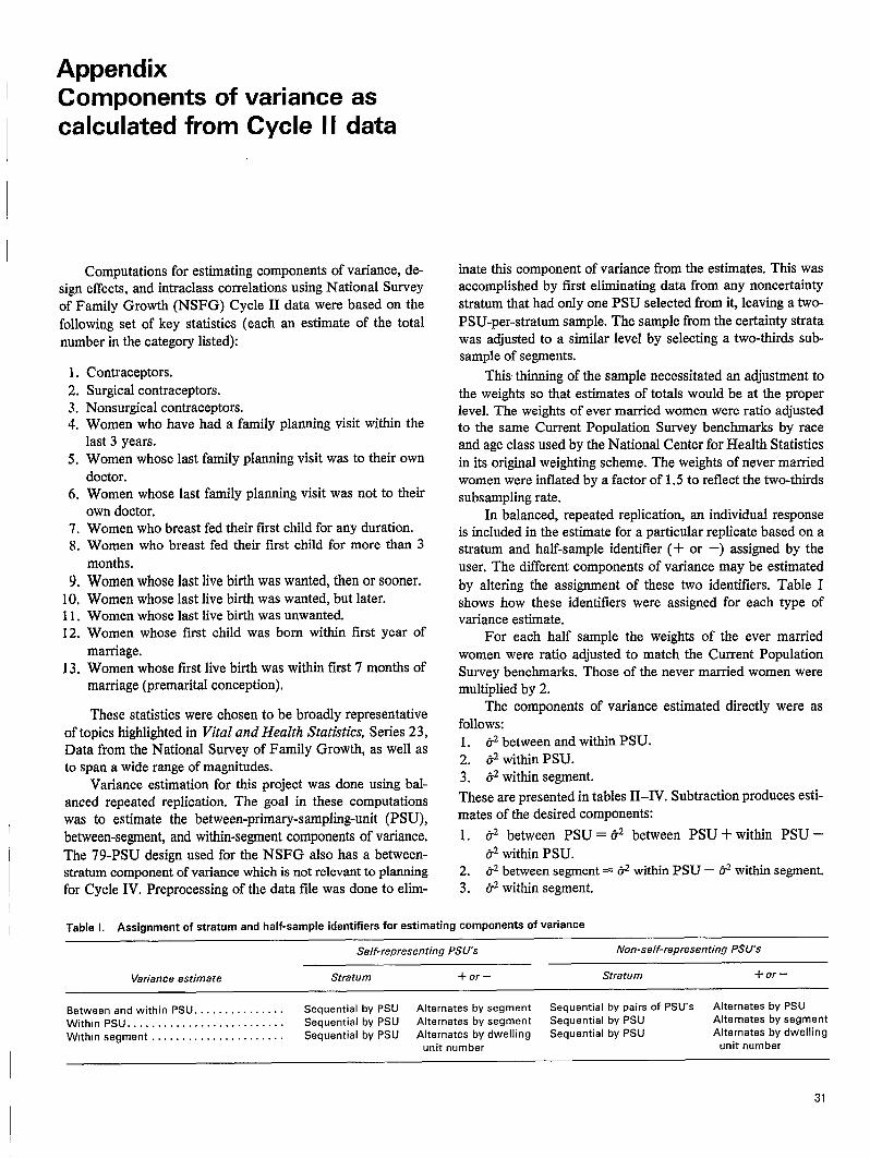
AppendixComponents of variance ascalculated from Cycle II data

I Computations for estimating components of variance, de-sign effects, and intraclass correlations using National Survey

I of Family Growth (NSFG) Cycle II data were based on thefollowing set of key statistics (each an estimate of the totalnumber in the categow listed):

1,2,3. .4.

5,

6,

7.8.

9.10,11.12.

13.

Contraceptors.Surgical contraceptors.Nonsurgical contraceptors.Women who have had a family planning visit within thelast 3 years.Women whose last family planning visit was to their owndoctor.Women whose last family planning visit was not to theirown doctor.Women who breast fed their first child for any duration.Women who breast fed their first child for more than 3months,Women whose last live birth was wanted, then or sooner.Women whose last live birth was wanted, but later.Women whose last live birth was unwanted.Women whose first child was born within first year ofmarriage.Women whose first live birth was within first 7 months ofmarriage (premarital conception),

These statistics were chosen to be broadly representativeof topics highlighted in Vital and Health Statistics, Series 23,Data from the National Survey of Family Growth, as well asto span a wide range of magnitudes.

Variance estimation for this project was done using bal-anced repeated replication. The goal in these computationswas to estimate the between-primary-sampling-unit (PSU),between-segment, and within-segment components of variance.The 79-PSU design used for the NSFG also has a between-stratum component of variance which is not relevant to planningfor Cycle IV. Preprocessing of the data file was done to elim-

inate this component of variance from the estimates. This wasaccomplished by first eliminating data from any noncertaintystratum that had only one PSU selected from it, leaving a twcEPSU-per-stratum sample. The sample from the certainty stratawas adjusted to a similar level by selecting a two-thirds sub-sample of segments.

This thinning of the sample necessitated an adjustment tothe weights so that estimates of totals would be at the properlevel. The weights of ever married women were ratio adjustedto the same Current Population Survey benchmarks by raceand age class used by the National Center for Health Statisticsin its original weighting scheme. The weights of never marriedwomen were inflated by a factor of 1.5 to reflect the two-thirdssubsampling rate.

In balanced, repeated replication, an individual responseis included in the estimate for a particular replicate based on astratum and half-sample identifier (+ or –) assigned by theuser. The different components of variance may be estimatedby altering the assignment of these two identifiers. Table Ishows how these identifiers were assigned for each type ofvariance estimate.

For each half sample the weights of the ever marriedwomen were ratio adjusted to match the Current PopulationSurvey benchmarks. Those of the never married women weremultiplied by 2.

The components of variance estimated directly were asfollows:1. $ between and within PSU.2. &2within PSU.3. $ within segment.

These are presented in tables II-IV. Subtraction produces esti-mates of the desired components:

1. @2between PSU = U2 between PSU + within PSU –&2within PSU.

2. & between segment= & within PSU – & within segment.3. r32within segment.

Table 1. Assignment of stratum and half-sample identifiers for estimating components of variance

Self-representing PSUs Non-self-representing PSU’S

Variance estimate Stratum +or– Stratum +or -

Between andwithin PSU . . . . . . . . . . . . . . . Sequential by PSU Alternates by segment Sequential by pairs of PSU’S Alternates by PSU

Within PSU . . . . . . . . . . . . . . . . . . . . . . . . . . Sequential by PSU Alternates by segment Saquantial by PSU Alternates by segment

Within segment . . . . . . . . . . . . . . . . . . . . . . Sequential by PSU Alternates by dwelling Sequential by PSU Alternates by dwelling

unit number unit number

31

Tabla Il. Cycle 11family growth variance estimates between and within PSU by race and categories of women

Standard Coeff/c/entRace and category of woman Estimate Variance error of variation

Black

Contraceptor . . . . . . . . . . . . . . . . . . . . . . . . . . . . . . . . . . . . . . . . . . . . . . . . . . . . . . . . . . .Surgical contraceptor . . . . . . . . . . . . . . . . . . . . . . . . . . . . . . . . . . . . . . . . . . . . . . . . . . . .Nonsurgical contraceptor . . . . . . . . . . . . . . . . . . . . . . . . . . . . . . . . . . . . . . . . . . . . . . . . .Had family planning visit within last 3 years . . . . . . . . . . . . . . . . . . . . . . . . . . . . . . . . . .Last family planning visit to own doctor . . . . . . . . . . . . . . . . . . . . . . . . . . . . . . . . . . . . .

Last family planning visit notto own doctor. . . . . . . . . . . . . . . . . . . . . . . . . . . . . . . . . .Breaatfad first child for any duration. . . . . . . . . . . . . . . . . . . . . . . . . . . . . . . . . . . . . . . .Breast fed first child formorethsn3 months . . . . . . . . . . . . . . . . . . . . . . . . . . . . . . . . .

Last live birth wantad, then or sooner. . . . . . . . . . . . . . . . . . . . . . . . . . . . . . . . . . . . . . .Last live birth wanted, but later.. . . . . . . . . . . . . . . . . . . . . . . . . . . . . . . . . . . . . . . . . . .Lsstlive birth unwanted . . . . . . . . . . . . . . . . . . . . . . . . . . . . . . . . . . . . . . . . . . . . . . . . . .First child born within first year of marriage . . . . . . . . . . . . . . . . . . . . . . . . . . . . . . . . . .Premarital conception . . . . . . . . . . . . . . . . . . . . . . . . . . . . . . . . . . . . . . . . . . . . . . . . . . . .

White and other

Contraceptor . . . . . . . . . . . . . . . . . . . . . . . . . . . . . . . . . . . . . . . . . . . . . . . . . . . . . . . . . . .Surgical contraceptor . . . . . . . . . . . . . . . . . . . . . . . . . . . . . . . . . . . . . . . . . . . . . . . . . . . .Nonsurgical contraceptor . . . . . . . . . . . . . . . . . . . . . . . . . . . . . . . . . . . . . . . . . . . . . . . . .Had family planning visit within last 3 years . . . . . . . . . . . . . . . . . . . . . . . . . . . . . . . . . .Last family planning visit to own doctor . . . . . . . . . . . . . . . . . . . . . . . . . . . . . . . . . . . . .

Last family planning visit notto own doctor. . . . . . . . . . . . . . . . . . . . . . . . . . . . . . . . . .Breast fed first child forany duration. . . . . . . . . . . . . . . . . . . . . . . . . . . . . . . . . . . . . . . .Breast fed first child for more than 3 months . . . . . . . . . . . . . . . . . . . . . . . . . . . . . . . . .

Last live birth wanted, then or sooner. . . . . . . . . . . . . . . . . . . . . . . . . . . . . . . . . . . . . . .Last live birth wanted, but later.. . . . . . . . . . . . . . . . . . . . . . . . . . . . . . . . . . . . . . . . . . .

Last live birth unwanted . . . . . . . . . . . . . . . . . . . . . . . . . . . . . . . . . . . . . . . . . . . . . . . . . .First child born within first year of marriage . . . . . . . . . . . . . . . . . . . . . . . . . . . . . . . . . .Premarital conception . . . . . . . . . . . . . . . . . . . . . . . . . . . . . . . . . . . . . . . . . . . . . . . . . . . .

2,420,093448,770

1,971,3231,724,061

B73,936732,971

1,004,225506,477

1,621,007‘1,040,1701,095,760

960,006659,907

19,588,1315,291,34014,296,79114,048,92011,340,357

2,115,512B,559,4173,BB5,143

14,457,69B5,196,351

3,283,5218,161,0224,132,640

8,48 B,948,5302,031,145,0306,507,505,5906,739,469,2305,340,103,0505,476,464,2003,820,354,840

2,422,454,3403,636,21 B,3603,370,875,7002,575,684,4604,145,065,4601,727,495,450

87,6B1 ,683,BO078,435,283,200

147,81 B,901 ,000116,884,02B,000130,425,806,000

27,960,381,60080,478,87 B,30038,372,987,70090,793,742,00058,795,618,70025,776,525,60072,369,758,40044,789,B41 ,600

92,13545,06880,66982,09473,07674,003

61 ,B0949,21860,3015B,05950,75164,3B241,563

296,1112B0,0633B4,472341,883361,145167,2142B3,68B195,890301,320242,478160,551269,016211,636

0.03B10.10040.04090.04760,0B360.1010

0.06150.09720.03720.05580.04630.06710.0630

0.01510.05290.02690.02430.031 B

0.07900.03310.05040.020?0.0467

0.04B90.03300.0512

Table I Il. Cycla II family growth variance estimates within PSU by rata and categories of women

Standard CoefficientRace and categoty of woman Estimate Variance error of variation

Black

Contraceptor . . . . . . . . . . . . . . . . . . . . . . . . . . . . . . . . . . . . . . . . . . . . . . . . . . . . . . . . . . .Surgical contraceptor . . . . . . . . . . . . . . . . . . . . . . . . . . . . . . . . . . . . . . . . . . . . . . . . . . . .Nonsurgical contraceptor . . . . . . . . . . . . . . . . . . . . . . . . . . . . . . . . . . . . . . . . . . . . . . . . .Had family planning visit within last 3 years . . . . . . . . . . . . . . . . . . . . . . . . . . . . . . . . . .Last family planning visit to own doctor . . . . . . . . . . . . . . . . . . . . . . . . . . . . . . . . . . .Last family planning visit not to own doctor . . . . . . . . . . . . . . . . . . . . . . . . . . . . . . . . . .Breast fed first child for any duration. . . . . . . . . . . . . . . . . . . . . . . . . . . . . . . . . . . . . . . .Breaatfed first child for more than 3 months . . . . . . . . . . . . . . . . . . . . . . . . . . . . . . . . .Last live birth wanted, then or sooner. . . . . . . . . . . . . . . . . . . . . . . . . . . . . . . . . . . . . . .

Lsst live birth wanted, but later . . . . . . . . . . . . . . . . . . . . . . . . . . . . . . . . . . . . . . . . . . . .

Last live birth unwanted . . . . . . . . . . . . . . . . . . . . . . . . . . . . . . . . . . . . . . . . . . . . . . . . . .First child born within first yearof marriage . . . . . . . . . . . . . . . . . . . . . . . . . . . . . . . . . .Premarital conception . . . . . . . . . . . . . . . . . . . . . . . . . . . . . . . . . . . . . . . . . . . . . . . . . . . .

White and other

Contraceptor . . . . . . . . . . . . . . . . . . . . . . . . . . . . . . . . . . . . . . . . . . . . . . . . . . . . . . . . . . .Surgical contraceptor . . . . . . . . . . . . . . . . . . . . . . . . . . . . . . . . . . . . . . . . . . . . . . . . . . . .Nonsurgical contraceptor . . . . . . . . . . . . . . . . . . . . . . . . . . . . . . . . . . . . . . . . . . . . . . . . .

Had family planning visit within last3 years . . . . . . . . . . . . . . . . . . . . . . . . . . . . . . . . . .

Last family planning visit to own doctor . . . . . . . . . . . . . . . . . . . . . . . . . . . . . . . . . . . . .Last family planning visit not to own doctor . . . . . . . . . . . . . . . . . . . . . . . . . . . . . . . . . .Breast fed first child for any duration. . . . . . . . . . . . . . . . . . . . . . . . . . . . . . . . . . . . . . . .Breast fed first child for more than 3 months . . . . . . . . . . . . . . . . . . . . . . . . . . . . . . . . .Last live birth wanted, then orsooner. . . . . . . . . . . . . . . . . . . . . . . . . . . . . . . . . . . . . . .Last live birth wanted, but later.. . . . . . . . . . . . . . . . . . . . . . . . . . . . . . . . . . . . . . . . . . .Last live birth unwanted . . . . . . . . . . . . . . . . . . . . . . . . . . . . . . . . . . . . . . . . . . . . . . . . . .First child born within first year of marriage . . . . . . . . . . . . . . . . . . . . . . . . . . . . . . . . . .Premarital conception . . . . . . . . . . . . . . . . . . . . . . . . . . . . . . . . . . . . . . . . . . . . . . . . . . . .

2,420,093448,770

1,971,3231,724,061

B73,936732,971

1,004,225506,477

1,621,007

1,040,1701,095,760

960,006659,907

19,588,1315,291,340

14,296,79114,048,920

11,340,3572,115,5128,559,4173,885,143

14,457,6985,196,3513,283,5218,161,0224,132,640

7,787,095,290925,867,998

5,233,55Z,1204, B03,545,3803,776,200,3903,377,039,7703,281,294,8402,453,951,6203,122,51 B,040

5,780,761,7202,740,103,0303,131,131,4501,404,540,040

71,375,266,10042,819,579,600

116,922,269,00047,340,573,300

55,332,845,20029,834,095,70056,243,023,40029,412,562,60042,1 4~,598,80045,471,006,20031,599,334,500

103,389,650,00050, B33,454,800

B8,24530,42872,34369,30861,45158,11257,28349,53755,B79

76,03152,34655,95737,477

267,161206,929

341,939217,579

235,229172,725237,156171,501205,287213,239177,762321,543225,463

0.03650.067B0.03670.04020.07030.07930.05700.09780.03450.07310.04780.05830.0568

0.01360.03910.0239

0.0155

0.0207O.OB160.02770.04410.01420.04100.05410.03940.0546

32

Table IV. Cycle I I family growth variance estimatea within segment by race and categories of women

Standard Coefficient

Race and catego~ of woman Estimate Variance error of variation

Black

Contraceptor . . . . . . . . . . . . . . . . . . . . . . . . . . . . . . . . . . . . . . . . . . . . . . . . . . . . . . . . . . .Surgical contracaplor . . . . . . . . . . . . . . . . . . . . . . . . . . . . . . . . . . . . . . . . . . . . . . . . . . . .Nonsurgical contraceptor . . . . . . . . . . . . . . . . . . . . . . . . . . . . . . . . . . . . . . . . . . . . . . . . .Had family planning visit within last3 years . . . . . . . . . . . . . . . . . . . . . . . . . . . . . . . . . .Last family planning visit to own doctor . . . . . . . . . . . . . . . . . . . . . . . . . . . . . . . . . . . . .Last family planning visit notto own doctor . . . . . . . . . . . . . . . . . . . . . . . . . . . . . . . . . .Breast fed first child for any duration. . . . . . . . . . . . . . . . . . . . . . . . . . . . . . . . . . . . . . . .Breast fed first child for more than 3 months . . . . . . . . . . . . . . . . . . . . . . . . . . . . . . . . .Last live birth wanted, then orsooner. . . . . . . . . . . . . . . . . . . . . . . . . . . . . . . . . . . . . . .Last live birth wanted, but later... . . . . . . . . . . . . . . . . . . . . . . . . . . . . . . . . . . . . . . . . .Last live birth unwanted . . . . . . . . . . . . . . . . . . . . . . . . . . . . . . . . . . . . . . . . . . . . . . . . . .Flrstchlld born within first year of marriage . . . . . . . . . . . . . . . . . . . . . . . . . . . . . . . . . .Premarital conception . . . . . . . . . . . . . . . . . . . . . . . . . . . . . . . . . . . . . . . . . . . . . . . . . . . .

White and other

Contracaptor, . . . . . . . . . . . . . . . . . . . . . . . . . . . . . . . . . . . . . . . . . . . . . . . . . . . . . . . . . .Surgical contraceptor . . . . . . . . . . . . . . . . . . . . . . . . . . . . . . . . . . . . . . . . . . . . . . . . . . . .Nonsurgical contraceptor . . . . . . . . . . . . . . . . . . . . . . . . . . . . . . . . . . . . . . . . . . . . . . . . .Had family planning visit within last3 years . . . . . . . . . . . . . . . . . . . . . . . . . . . . . . . . . .Last family planning visit to own doctor . . . . . . . . . . . . . . . . . . . . . . . . . . . . . . . . . . . . .

Last family planning visit notto own doctor . . . . . . . . . . . . . . . . . . . . . . . . . . . . . . . . . .Breast fed first child forany duration. . . . . . . . . . . . . . . . . . . . . . . . . . . . . . . . . . . . . . . .Breast fed first child formore than 3 months . . . . . . . . . . . . . . . . . . . . . . . . . . . . . . . . .Last live birth wanted, then or sooner . ..!..... . . . . . . . . . . . . . . . . . . . . . . . . . . . . . .

Last live birth wanted, but later . . . . . . . . . . . . . . . . . . . . . . . . . . . . . . . . . . . . . . . . . . . .

Last live birth unwanted . . . . . . . . . . . . .,, ..,...! . . . . . . . . . . . . . . . . . . . . . . . . . . . .

First child born within first yearof marriage . . . . . . . . . . . . . . . . . . . . . . . . . . . . . . . . . .Premarital conception . . . . . . . . . . . . . . . . . . . . . . . . . . . . . . . . . . . . . . . . . . . . . . . . . . . .

2,420,09344 B,770

1,971,3231,724,061

873,936732,971

1,004,225506,477

1,621,0071,040,1701,095,760

960,006659,907

19,5BB,1 315,291,340

14.296,79114,04B,92011,340,357

2,115,5128,559,4173,885,143

14,457,6985,196,351

3,2 B3,5218,161,0224,132,640

3,412,625,930682,522,0B3

3,068,381,0903,725,432,7503,049,227,4503,410,762,6702,370,040,2601,204,912,1903,479,479,7405,176,962,6102,662,B1 1,9602,3BI ,227,7502,110,942,500

40,609,652,60053,530,084,20052,746,445,80050,224,706,10046,314,146,00014,661,6 B5,90064,122,743,70038,1 26,3BB,10080,367,974,BO048,889,710,300

27,654, B8B,I 0035,522,609,20031,363,390,400

58,41826,125

55,39361,03655,2205B,4024B,68334,71258,9B771,95151,60248,79B45,945

201,518231,366229,666224,109215,207121,085253,225195,260283,492221,110

166,298188,474177,097

0.02410.05B20.02810.03540.06320.07970.04B50.06850.03640.06920.04710.05080.0696

0.01030.04370.01610.01600.0190

0.05720.02960.05030.01960.0426

0.05060.02310.0429

The percent of the total variance attributable to each componentis presented in table V. (Note that some estimates are negative.)Average values calculated separately for the black and for thewhite and other races subgroups are presented in table VI.

Design effects were estimated for each item as

d2 withh segment ~ Q‘EFF = (Estimated total)2 nP

Cvcle II relvariance—,.= Relvariance under simple random sampling

where n = effective sample size from the subpopulation (blackor white and other eligible women)

P = estimated total expressed as a proportion of thesubpopulation total

Q=l– P

(All the items for which variances were calculated are countsof women, and thus QhP is the variance estimator with simplerandom sampling.) These variables are presented item by itemin table VII. Averages by race of DEFF’s are given in tableVIII.

As described earlier, ratio adjusting of sampling weightswas performed only on the ever married group. In Cycle II ofNSFG, the only never married women eligible for interviewingwere those who had children and whose children lived withthem in their home. There was no accepted count of thesewomen nationally, so their estimated total in Cycle II could notbe benchmarked.

In Cycle IV of NSFG, all women between the ages of 15and 44 will be considered eligible without regard to maritalstatus as was the case in Cycle III. Because there are varianceimplications associated within ratio adjusting and because inCycle IV adjustments will be made for both the ever marriedand never married groups, the variance calculations were re-peated and the weights were ratio adjusted within each replicatefor both ever married and never married women. The nevermarried group was benchmarked to the Ml dataset estimatesby race and age class. The revised figures can be found intables IX–XV. These variances most closely reflect the sam-pling and estimation procedure to be used in Cycle IV and arethe ones used in the analyses.

While the estimated average design effect for both racialgroups showed some reduction relative to the earlier estimates,the most dramatic change occurred in the estimated componentsof variance for the black subgroup. There the proportion of thetotal variance contributed by the between-PSU componentdropped from 13.1 to 0.7 percent.

33

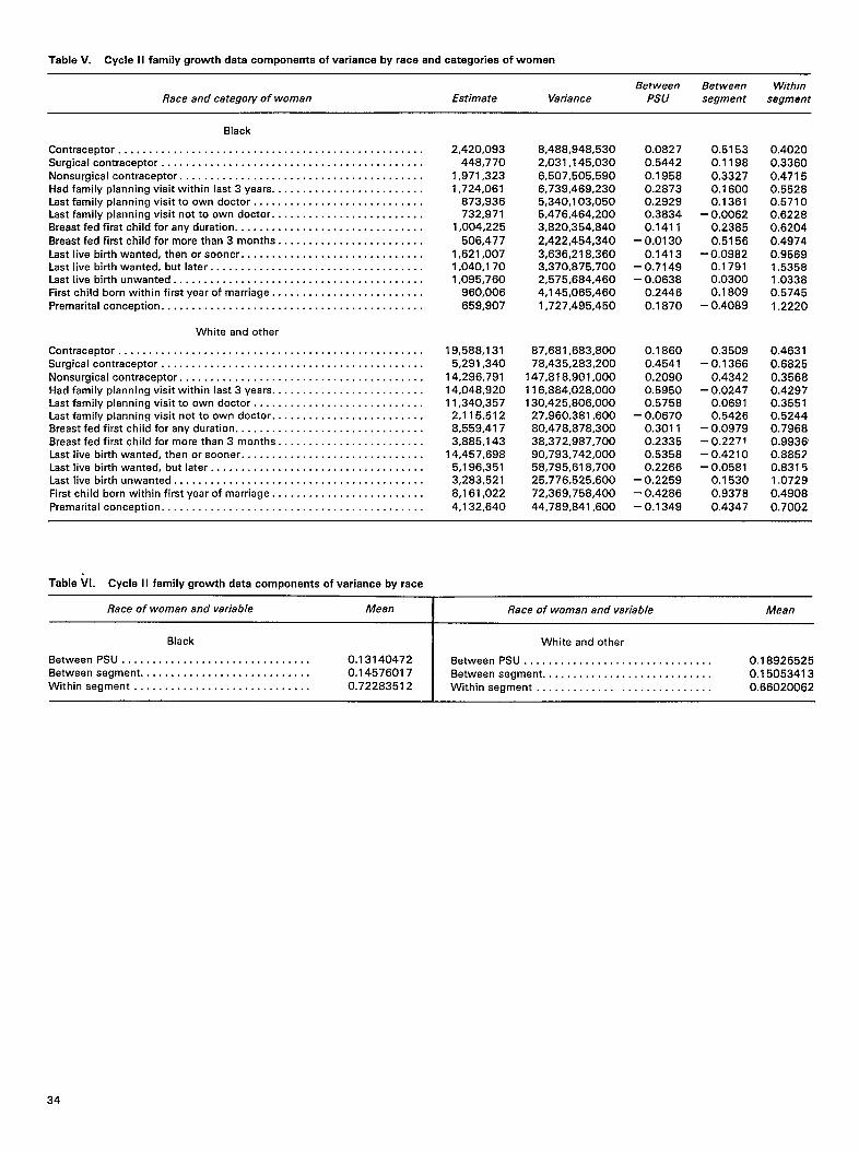
Table V. Cycle II famiIy growth data components of variance by race and categories of women

Between Between WithinRace and catego~ of woman Estimate Variance Psu segment segment

Black

Contraceptor . . . . . . . . . . . . . . . . . . . . . . . . . . . . . . . . . . . . . . . . . . . . . . . . . .Surgical contraceptor . . . . . . . . . . . . . . . . . . . . . . . . . . . . . . . . . . . . . . . . . . .Nonsurgical contraceptor . . . . . . . . . . . . . . . . . . . . . . . . . . . . . . . . . . . . . . . .Had family planning visit within last 3 yeara. . . . . . . . . . . . . . . . . . . . . . . . .Last family planning visit to own doctor . . . . . . . . . . . . . . . . . . . . . . . . . . . .Lest family planning visit not to own doctor . . . . . . . . . . . . . . . . . . . . . . . . .Breast fed first child forany duration. . . . . . . . . . . . . . . . . . . . . . . . . . . . . . .Breast fed first child formorethan3 months . . . . . . . . . . . . . . . . . . . . . . . .Last live birth wanted, then or sooner . . . . . . . . . . . . . . . . . . . . . . . . . . . . . .

Last live bitihwanted, but later.. . . . . . . . . . . . . . . . . . . . . . . . . . . . . . . . . .Last live birth unwanted . . . . . . . . . . . . . . . . . . . . . . . . . . . . . . . . . . . . . . . . .First child born within firatyear of marriage. . . . . . . . . . . . . . . . . . . . . . . . .

Premarital conception . . . . . . . . . . . . . . . . . . . . . . . . . . . . . . . . . . . . . . . . . . .

White end other

Contraceptor . . . . . . . . . . . . . . . . . . . . . . . . . . . . . . . . . . . . . . . . . . . . . . . . . .Surgical contraceptor . . . . . . . . . . . . . . . . . . . . . . . . . . . . . . . . . . . . . . . . . . .

Nonsurgical contraceptor . . . . . . . . . . . . . . . . . . . . . . . . . . . . . . . . . . . . . . . .Had family planning visit within last 3 years. . . . . . . . . . . . . . . . . . . . . . . . .Last family planning visit to own doctor . . . . . . . . . . . . . . . . . . . . . . . . . . . .Last family planning visit not to own doctor . . . . . . . . . . . . . . . . . . . . . . . . .Breast fed first child for any duration. . . . . . . . . . . . . . . . . . . . . . . . . . . . . . .Breast fed first child formorathan3 months . . . . . . . . . . . . . . . . . . . . . . . .

Last live birth wanted, then orsooner. . . . . . . . . . . . . . . . . . . . . . . . . . . . . .Last live birth wanted, but later.. . . . . . . . . . . . . . . . . . . . . . . . . . . . . . . . . .

Last live birth unwanted . . . . . . . . . . . . . . . . . . . . . . . . . . . . . . . . . . . . . . . . .First child born within first year of marriage . . . . . . . . . . . . . . . . . . . . . . . . .

Premarital conception . . . . . . . . . . . . . . . . . . . . . . . . . . . . . . . . . . . . . . . . . . .

2,420,09344B,770

1,977,3231,724,061

B73,936732,971

1,004,225

506,4771,621,0071,040,1701,095,760

960,006

659,907

19,5BB,1 315,291,340

14,296,79114,048,920‘17,340,357

2,115,512B,559,4173,885,143

14,457,6985,196,3513,283,5218,161,022

4,132,640

8,4 B8,94B,5302,031,145,030

6,507,505,5906,739,469,2305,340,103,0505,476,464,2003,820,354,840

2,422,454,3403,636,21 B,3603,370,875,7002,575,684,4604,145,065,460

1,727,495,450

B7,681 ,683,80078,435,283,200

147,818,901,000116,884,028,000130,425,806,000

27,960,381,60080,478, B7B,30038,372,987,70090,793,742,0005B,795.61 8,70025,776,525,60072,369,758,400

44,789,841,600

0.08270.54420.19580.2B730.29290.3B340.1411

– 0.01300.1413

–0.7149– 0.063B

0.24460.1870

0.18600.45410.20900.59500.5758

– 0.06700.30110.23350.53580.2266

– 0.2259– 0.42B6

– 0.1349

0.51530.119B0.33270.16000.1361

– 0.00620.2385

0.5156- 0.09B2

0.17910.03000.1 B09

-0.4089

0.3509-0.1366

0.4342– 0.0247

0.06910.5426

– 0.0979- 0.2z7q

-0.4210– 0.0581

0.15300.9378

0.4347

0.40200.3360

0.47150.55280.57100.62280.6204

0.49740.95691.53581.033B0.5745

1.2220

0.46310.68250.356B0.42970.35510.52440.796B0.99360.88570.83151.0729

0.4908

0.7002

Table V1. Cycle II femily growth data components of variance by race

Race of woman and variable Mean1

Race of woman and variable Mean

Black I White and othar

Betwean PSU . . . . . . . . . . . . . . . . . . . . . . . . . . . . . . . 0.13140472

I Between PSU . . . . . . . . . . . . . . . . . . . . . . . . . . . . . . . 0.18926526Betwean sagment . . . . . . . . . . . . . . . . . . . . . . . . . . . . 0.14576017 Between segment . . . . . . . . . . . . . . . . . . . . . . . . . . . . 0.15053413Within segment . . . . . . . . . . . . . . . . . . . . . . . . . . . . . 0.72283512 Within segment . . . . . . . . . . . . . . . . . . . . . . . . . . . . 0.66020062

34

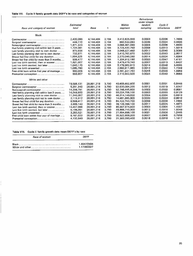
Table VI 1. Cycle II family growth data DEFF’s by race and catagoriea of women

Relvariancaunder simple

Estimated Within random Cycle IIRace and category of woman total Base n segment sampling relvariance DEFF

Black

Ccmtraceptor . . . . . . . . . . . . . . . . .. c.. . . . . . .Surgical contraceptor . . . . . . . . . . . . . . . . . . . .

Nonsurgical contraceptor . . . . . . . . . . . . . . . . .Had family planning visit within last 3 years. . .

Last family planning visit to own doctor . . . . .

Last family planning visit not to own doctor. . .Breast fed first child for any duration. . . . . . . .

Breast fed first child for more than 3 months. . .Last Iwe birth wanted, then or sooner. . . . . . .

Last Iwe birth wanted, but later . . . . . . . . . . . .

Laatlive birth unwanted . . . . . . . . . . . . . . . . . .First child born within first year of marriage . . .Premarital conception . . . . . . . . . . . . . . . . . . . .

White and other

Contraceptor . . . . . . . . . . . . . . . . . . . . . . . . . . .

Surgical contraceptor . . . . . . . . . . . . . . . . . . . .Nonsurgical contraceptor . . . . . . . . . . . . . . . . .Had family planning visit within last 3 years. . .Last family planning visit to own doctor . . . . .

Last family planning visit not to own doctor. . .

Breast fed first child for any duration. . . . . . . .

Breast fed first child for more than 3 months. . .Last live birth wanted, then or sooner. . . . . . .

Last live birth wanted, but later . . . . . . . . . . . .Last live birth unwanted . . . . . . . . . . . . . . . . .First child born within first year of marriaga . . .Premarital conception . . . . . . . . . . . . . . . . . . . .

2,420,093448,770

1,971,3231,724,061

873,936732,971

1,004,225

506,4771,621,007

1,040,1701,095,760

960,006659,907

19,588,131

5,291,34014,296,79114,048,92011,340,357

2,115,512

8,559,417

3,885,14314,457,698

5,196,351

3,283,5218,161,022

4,132,640

4,144,4644,144,464

4,144,4644,144,464

4,144,464

4,144,464

4,144,464

4,144,4644,144,464

4,144,4644,144,4644,144,464

4,144,464

28,B91 ,21 B

28,891,218

28,891,21828,891,21828,891,218

28,891,21828,891,218

28,891,21828,891,21828,891,218

28,891,21828,891,218

28,891,218

2,164

2,164

2,1642,164

2,1642,164

2,164

2,1642,164

2,1642,164

2,1642,164

3,790

3,7903,7903,7903,790

38790

3,790

3,7903,7903,790

3,7903,790

3,790

3,412,625,930

682,522,083

3,068,381,0903,725,432,750

3,049,227,4503,410,762,670

2,370,040,260

1,204,912,1903,479,479,7405,176,962,6102,662,811,960

2,381,227,7502,110,942,500

40,609,652,600

53,530,084,20052,746,445,80050,224,706,10046,314,146,000

14,661,685,900

64,122,743,700

38,126,388,10080,367,974,80048,889,710,300

27,654,888,10035.522.609,200

31.363,390,400

0.0003

0.0038

0.00050.0006

0.00170.0022

0.0014

0.00330.0007

0.00140.0013

0.00150.0024

0.0001

0.0012

0.00030.00030.0004

0.00330.0006

0.00170.00030.00120.00210.0007

0.0016

0.0006

0.0034

0.00080.00130.0040

0.0063

0.0024

0.00470.0073

0.00480.0022

0.00260.0048

0.0001

0.0019

0.00030.00030.0004

0.0033

0.0009

0.00250.00040.00180.00260.0005

0.0018

1.7696

0.89051.65001.9319

2.30862.9517

1.6264

1.41511.8407

3.46951.7249

1.68561.9866

0.8446

1.6247

0.95810.91290.8819

0.98101.3965

1.48731.45971.5049

1.24650.7958

1.1617

Table WI 1. Cycle II family growth data mean DEFF’a by race

Race of woman DEFF

Black . . . . . . . . . . . . . . . . . . . . . . . . . . . . . . . . . . . . . . 1.93470594

White and other . . . . . . . . . . . . . . . ...!. . . . . . . . . . 1.17350327

35

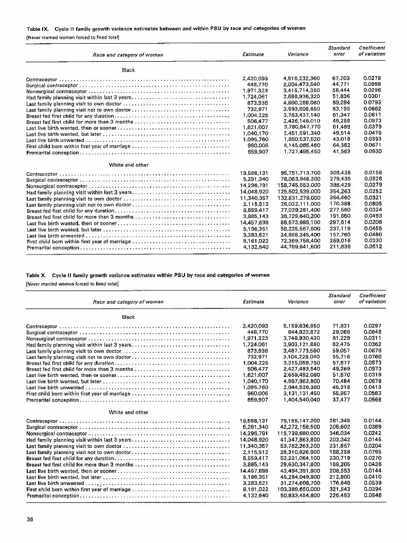
Table IX. Cycle II family growth variance estimates betwaen and within PSU by race and categories of women

[Never reamed women forced to fixed total]

Standard Coefficient

Race and category of woman Estimate Variance error of variation

Black

Contraceptor . . . . . . . . . . . . . . . . . . . . . . . . . . . . . . . . . . . . . . . . . . . . . . . . . . . . . . . . . . .Surgical contraceptor . . . . . . . . . . . . . . . . . . . . . . . . . . . . . . . . . . . . . . . . . . . . . . . . . . . .Nonsurgical contraceptor . . . . . . . . . . . . . . . . . . . . . . . . . . . . . . . . . . . . . . . . . . . . . . . . .Had family planning visit within last 3 years . . . . . . . . . . . . . . . . . . . . . . . . . . . . . . . . . .Last family planning visit to own doctor . . . . . . . . . . . . . . . . . . . . . . . . . . . . . . . . . . . . .Last family planning visit not to own doctor . . . . . . . . . . . . . . . . . . . . . . . . . . . . . . . . . .Breast fed first child for any duration. . . . . . . . . . . . . . . . . . . . . . . . . . . . . . . . . . . . . . . .Breast fed first child for more than 3 months . . . . . . . . . . . . . . . . . . . . . . . . . . . . . . . . .Last live birth wanted, then or sooner. . . . . . . . . . . . . . . . . . . . . . . . . . . . . . . . . . . . . . .Last live birth wanted, but later... . . . . . . . . . . . . . . . . . . . . . . . . . . . . . . . . . . . . . . . . .Last live birth unwanted . . . . . . . . . . . . . . . . . . . . . . . . . . . . . . . . . . . . . . . . . . . . . . . . . .First child born within first year of marriage . . . . . . . . . . . . . . . . . . . . . . . . . . . . . . . . . .Premarital conception . . . . . . . . . . . . . . . . . . . . . . . . . . . . . . . . . . . . . . . . . . . . . . . . . . . .

White and other

Contraceptor . . . . . . . . . . . . . . . . . . . . . . . . . . . . . . . . . . . . . . . . . . . . . . . . . . . . . . . . . . .Surgical contraceptor . . . . . . . . . . . . . . . . . . . . . . . . . . . . . . . . . . . . . . . . . . . . . . . . . . . .Nonsurgical contraceptor . . . . . . . . . . . . . . . . . . . . . . . . . . . . . . . . . . . . . . . . . . . . . . . . .

Had fsmilyplanning visit within last3 years . . . . . . . . . . . . . . . . . . . . . . . . . . . . . . . . . .Lsstfamily planning visit to own doctor . . . . . . . . . . . . . . . . . . . . . . . . . . . . . . . . . . . . .Last family planning visit not to own doctor . . . . . . . . . . . . . . . . . . . . . . . . . . . . . . . . . .Breast fed first child for any duration. . . . . . . . . . . . . . . . . . . . . . . . . . . . . . . . . . . . . . . .Breast fed firatchild formorethan3 months . . . . . . . . . . . . . . . . . . . . . . . . . . . . . . . . .Last live birth wanted, then or sooner . . . . . . . . . . . . . . . . . . . . . . . . . . . . . . . . . . . . . . .

Last live birth wanted, but later.. . . . . . . . . . . . . . . . . . . . . . . . . . . . . . . . . . . . . . . . . . .Last live birth unwanted . . . . . . . . . . . . . . . . . . . . . . . . . . . . . . . . . . . . . . . . . . . . . . . . . .First child born within first year of marriage . . . . . . . . . . . . . . . . . . . . . . . . . . . . . . . . . .Premarital conception . . . . . . . . . . . . . . . . . . . . . . . . . . . . . . . . . . . . . . . . . . . . . . . . . . . .

2,420,093448,770

1,971,3231,724,061

873,936732,971

1,004,225506.477

1,621,0071,040,1701,095,760

960,006659,907

19,588,1315,291,340

14,296,791

14,048,92011,340,357

2,115,5128,559,4173,885,143

14,457,698

5,196,3513,283,5218,161,0224,132,640

4,516,232,3602,004,473,5403,415,714,3602,686,936,3204,800,288,0603,993,605,6503,763,437,1402,426,146,0103,780,847,770

2,451,591,3401,850,537,5204,145,065,4601,727,495,450

95,751,713,70078,083,948,300

158,745,583,000

125,502,539,000

132,831,276,00029,032,111,00077,039,281,40036,729,640,200

88,573,985,10056,225,567,60024,888,345,40072,369,758,40044,789,841,600

67,20344,77158,44451,83669,28463,19561,34749,25661 ,4B949,51443,01864,38241,563

309,438279,435398,429

354,263364,460170,388277,560191,650297,614

237,119157,760269,016211,636

0.02780.09980.02960.0301

0.07930.08620.06110.09730.03790.04760.03930.06710.0630

0.01580.05280.0279

0.02520.03210.08050.03240,0493

0.02060.04560.04800.03300.0512

Table X. Cycle II family growth varience estimates within PSU by rata and categories of women

[Never married women forced to fixed total]

Standard CoefficientRace and category of woman Estimate Variance error of varietion

Black

Contraceptor . . . . . . . . . . . . . . . . . . . . . . . . . . . . . . . . . . . . . . . . . . . . . . . . . . . . . . . . . . .Surgical contraceptor . . . . . . . . . . . . . . . . . . . . . . . . . . . . . . . . . . . . . . . . . . . . . . . . . . . .Nonaurgicel contraceptor . . . . . . . . . . . . . . . . . . . . . . . . . . . . . . . . . . . . . . . . . . . . . . . . .

Had family planning visit within last3 years . . . . . . . . . . . . . . . . . . . . . . . . . . . . . . . . . .Last family planning viaitto own doctor . . . . . . . . . . . . . . . . . . . . . . . . . . . . . . . . . . . . .Last family planning visit not to own doctor . . . . . . . . . . . . . . . . . . . . . . . . . . . . . . . . . .Breast fed first child for any duration. . . . . . . . . . . . . . . . . . . . . . . . . . . . . . . . . . . . . . . .Breast fed first child for more than 3 months . . . . . . . . . . . . . . . . . . . . . . . . . . . . . . . . .

Last livabirth wanted, then or sooner . . . . . . . . . . . . . . . . . . . . . . . . . . . . . . . . . . . . . . .Last livabirth wsnted, but later... . . . . . . . . . . . . . . . . . . . . . . . . . . . . . . . . . . . . . . . . .Lest live birth unwanted . . . . . . . . . . . . . . . . . . . . . . . . . . . . . . . . . . . . . . . . . . . . . . . . . .First child born within first year of marriage . . . . . . . . . . . . . . . . . . . . . . . . . . . . . . . . . .Premarital conception . . . . . . . . . . . . . . . . . . . . . . . . . . . . . . . . . . . . . . . . . . . . . . . . . . . .

White and other

Contraceptor . . . . . . . . . . . . . . . . . . . . . . . . . . . . . . . . . . . . . . . . . . . . . . . . . . . . . . . . . . .Surgical contraceptor . . . . . . . . . . . . . . . . . . . . . . . . . . . . . . . . . . . . . . . . . . . . . . . . . . . .

Nonsurgical contraceptor . . . . . . . . . . . . . . . . . . . . . . . . . . . . . . . . . . . . . . . . . . . . . . . . .

Had family planning visit within last3 years . . . . . . . . . . . . . . . . . . . . . . . . . . . . . . . . . .Lest family plsnning visit to own doctor . . . . . . . . . . . . . . . . . . . . . . . . . . . . . . . . . . . . .Lest family planning visit not to own doctor . . . . . . . . . . . . . . . . . . . . . . . . . . . . . . . . . .Breast fed first child for any duration. . . . . . . . . . . . . . . . . . . . . . . . . . . . . . . . . . . . . . . .

Breast fed first child formorethan3 months . . . . . . . . . . . . . . . . . . . . . . . . . . . . . . . . .

Last live birth wanted, then orsooner. . . . . . . . . . . . . . . . . . . . . . . . . . . . . . . . . . . . . . .Last live birth wanted, but later.. . . . . . . . . . . . . . . . . . . . . . . . . . . . . . . . . . . . . . . . . . .Last live birth unwanted . . . . .. .. . . . . . . . . . . . . . ...!.... . . . . . . . . . . . . . . . . . . . . . . .First child born within first year of marriage . . . . . . . . . . . . . . . . . . . . . . . . . . . . . . . . . .Premarital conception . . . . . . . . . . . . . . . . . . . . . . . . . . . . . . . . . . . . . . . . . . . . . . . . . . . .

2,420,093448,770

1,971,3231,724,061

873,936732,971

1,004,225506,477

1,621,007

1,040,1701,095,760

960,006

659,907

19,588,131

5,291,340

14,296,79114,048,920

11,340,3572,115,5128,559,4173,885,143

14,457,6985,196,3513,283,5218,161,0224,132,640

5,159,636,950844,823,872

3,748,930,430

3,903,121,8803,487,773,5803,104,228,0403,315,059,7502,427,483,5402,659,492,0804,967,963,8002,044,526,3603,131,131,4501,404,540,040

79,155,147,20042,272,158,500

119,739,680,00041,347,863,800

53,762,263,20028,310,826,90053,231,064,100

28,630,347,800

43,494,391,80045,284,049,80031,274,608,700

103,389,650,00050,833,454,800

71,83129,06661,22962,475

59,05755,71657,57749,26951,57070,48445,21655,957

37,477

281,345

205,602

346,034203,342

231,867168,258230,719

169,205

208,553212,800176,846321,543225,463

0.02970.064B0.03110.03620.06760.07600.05730.09730.031 B0.06780.04130.05B3

0.0568

0.0144

0.0369

0.02420.0145

0.02040.07950.0270

0.0436

0.01440.04100.05390.03940.0546

36

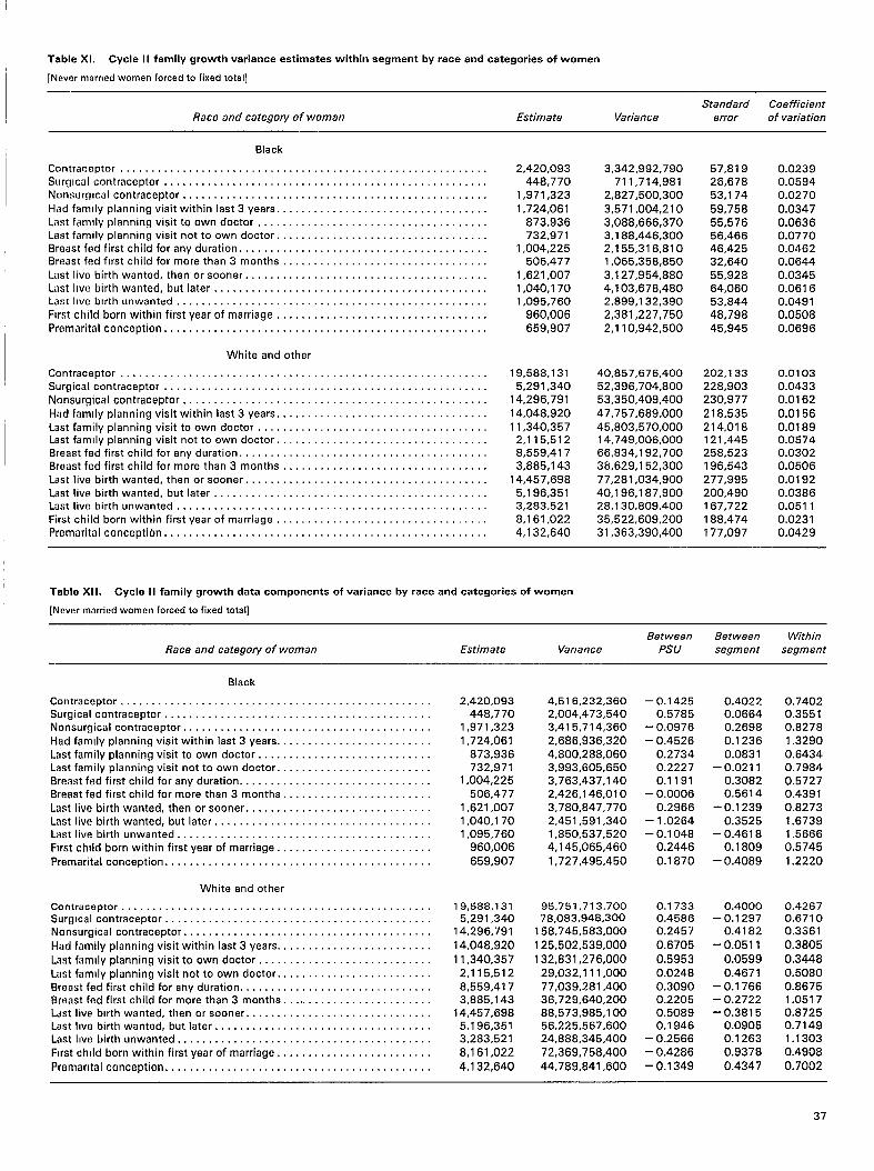
I

Table Xl. Cycle I I family growth variance eatimatea within segment by race and categories of women

[Nwer married women forced to fixed total]

~ Race and category of woman Estimate VarianceStandard Coefficient

error of variation

Black

Contraceptor . . . . . . . . . . . . . . . . . . . . . . . . . . . . . . . . . . . . . . . . . . . . . . . . .Surgical contraceptor . . . . . . . . . . . . . . . . . . . . . . . . . . . . . . . . . . . . . . . . . . . . . . . . . . . .Nonsurgical contraceptor . . . . . . . . . . . . . . . . . . . . . . . . . . . . . . . . . . . . . . . . . . . . . . . . .Had famllypianning visit within last 3 years . . . . . . . . . . . . . . . . . . . . . . . . . . . . . . . . . .

Last famllyplanning visit to own doctor . . . . . . . . . . . . . . . . . . . . . . . . . . . . . . . . . . . . .Last family planning visit notto own doctor . . . . . . . . . . . . . . . . . . . . . . . . . . . . . . . . . .Breast fed first child for any duration. . . . . . . . . . . . . . . . . . . . . . . . . . . . . . . . . . . . . . . .Breast fed flrstchild for more than 3 months . . . . . . . . . . . . . . . . . . . . . . . . . . . . . . . . .

Last live birth wanted, then or sooner . . . . . . . . . . . . . . . . . . . . . . . . . . . . . . . . . . . . . . .Last llvebirth wanted, but later... . . . . . . . . . . . . . . . . . . . . . . . . . . . . . . . . . . . . . . . . .Last lwebtrth unwanted . . . . . . . . . . . . . . . . . . . . . . . . . . . . . . . . . . . . . . . . . . . . . . . . . .Fmstchild born within first year of marriage . . . . . . . . . . . . . . . . . . . . . . . . . . . . . . . . . .Premarital conception, , .,,...... . . . . . . . . . . . . . . . . . . . . . . . . . . . . . . . . . . . . . . . . .

White and other

Contraceptor . . . . . . . . . . . . . . . . . . . . . . . . . . . . . . . . . . . . . . . . . . . . . . . . . . . . . . . . . . .Surgical contraceptor . . . . . . . . . . . . . . . . . . . . . . . . . . . . . . . . . . . . . . . . . . . . . . . . . . . .

Nonsurgical contraceptor . . . . . . . . . . . . . . . . . . . . . . . . . . . . . . . . . . . . . . . . . . . . . . . . .

Had famllyplanning visit within last3 years . . . . . . . . . . . . . . . . . . . . . . . . . . . .Last family planning visit to own doctor . . . . . . . . . . . . . . . . . . . . . . . . . . . . . . . . . . . . .Last famllyplanning visit not to own doctor . . . . . . . . . . . . . . . . . . . . . . . . . . . . . . . . . .Breast fed first child for any duration. . . . . . . . . . . . . . . . . . . . . . . . . . . . . . . . . . . . . . . .Breast fed first child formorethan3 months . . . . . . . . . . . . . . . . . . . . . . . . . . . . . . . . .

Last live birth wanted, then or sooner . . . . . . . . . . . . . . . . . . . . . . . . . . . . . .Last live birth wanted, but later.. . . . . . . . . . . . . . . . . . . . . . . . . . . . . . . . . . . . . . . . . . .Last live birth unwanted . . . . . . . . . . . . . . . . . . . . . . . . . . . . . . . . . . . . . . . . . . . . . . . . . .First child born within first year of marriage . . . . . . . . . . . . . . . . . . . . . . . . . . . . . . .Premarital conception ..,.......<.. . . . . . . . . . . . . . . 4 . . . . . . . . . . . . . . . . . . . . . . . .

2,420,093

448,770,971,323

,724,061873,936732,971

,004,225506,477

,621,007,040,170,095,760960,006

659,907

19,588,1315,291,340

14,296,791

14,048,920

11,340,3572,115,5128,559,4173,885,143

14,457,698

5,196,3513,283,5218,161,0224,132,640

3,342,992,790

711,714,981

2,827,500,300

3,571,004,210

3,088,666,370

3,188,446,300

2,155,316,810

1,065,358,850

3,127,954,880

4,103,678,480

2,899,132,390

2,381,227,750

2,110,942,500

40,857,676,40052,396,704,80053,350,409,40047,757,689,000

45,803,570,00014,749,006,00066,834,192,70038,629,152,300

77,281,034,90040,196,187,90028,130,809,40035,522,609,20031,363,390,400

57,819

26,678

53,174

59,758

55,576

56,466

46,425

32,640

55,928

64,060

53.844

48,798

45,945

202,133228,903230,977

218,535214,018121,445258,523196,543

277,995200,490167,722

188,474177,097

0.02390.05940.0270

0.03470.06360.07700.04620.06440.03450.06160.04910.05080.0696

0.01030.04330.0162

0.01560.01890.05740.03020.05060.01920.03860.05110.02310.0429

Table X11. Cycle I I family growth data components of variance by race and categories of women


Between Between WithinRace and categoiy of woman Estimate Variance Psu segment segment

81ack

Contraceptor . . . . . . . . . . . . . . . . . . . . . . . . . . . . .Surgical contraceptor . . . . . . . . . . . . . . . . . . . . . . . . . . . . . . . . . . . . . . . . . . .Nonsurgical contraceptor . . . . . . . . . . . . . . . . . . . . . . . . . . . . . . . . . . . . . . . .

Had family planning visit within last 3 years. . . . . . . . . . . . . . . . . . . . . . . . .Last family planning visit to own doctor . . . . . . . . . . . . . . . . . . . . . . . . . . . .Last family planning visit not to own doctor . . . . . . . . . . . . . . . . . . . . . . . . .Breast fed first child for any duration. . . . . . . . . . . . . . . . . . . . . . . . . . . . . . .Breast fed first child for more than 3 months . . . . . . . . . . . . . . . . . . . . . .

Last live birth wanted, then or sooner. . . . . . . . . . . . . . . . . . . . . . . . . . . . .

Last live birth wanted, but later.. . . . . . . . . . . . . . . . . . . . . . . . . . . . . . . . . .Last live birth unwanted . . . . . . . . . . . . . . . . . . . . . . . . . . . . . . . . . . . .First chlldborn within first year of marriage. . . . . . . . . . . . . . . . . . . . . . . . .

Premarital conception . . . . . . . . . . . . . . . . . . . . . . . . . . . . . . . . . . . . . . . . . .

White and other

Contraceptor . . . . . . . . . . . . . . . . . . . . . . . . . . . . . . . . . . . . . . . . . . . . . .Surgical contraceptor . . . . . . . . . . . . . . . . . . . . . . . . . . . . . . . . . . . . . . . . . .Nonsurgical contraceptor . . . . . . . . . . . . . . . . . . . . . . . . . . . . . . . . . . . . . . . .

Had family planning visit within last3 years. . . . . . . . . . . . . . . . . . . . . . . . .

Last famllyplanning visit to own doctor . . . . . . . . . . . . . . . . . . . . . . . . . . . .Last famtlyplanning viaitnot to own doctor. . . . . . . . . . . . . . . . . . . . . . . . .Breast fed first child for any duration. . . . . . . . . . . . . . . . . . . . . . . . . . . . . . .8reastfed first child for more than 3 months . . . .. . . . . . . . . . . . . . . . . . . . .Last live blrthwanted, then or sooner. . . . . . . . . . . . . . . . . . . . . . . . . . . . . .Last lwebirth wanted, but later.. . . . . . . . . . . . . . . . . . . . . . . . . . . . . . . . . .Last lwe birth unwanted . . . . . . . . . . . . . . . . . . . . . . . . . . . . . . . . . . . . . . . . .

Flrstchlld born within first yearof marriage . . . . . . . . . . . . . . . . . . . . . . . . .

Premtmtalc onception . . . . . . . . . . . . . . . . . . . . . . . . . . . . . . . . . . . . . . . . . . .

2,420,093448,770

1,971,323

1,724,061873,936732,971

1,004,225506,477

1,621,0071,040,1701,095,760

960,006

659.907

19,588,1315,291,340

14,296,791

14,048,920

11,340,357

2,115,5128,559,4173,885,143

14,457,6985,196,3513,283,521

8,161,022

4,132,640

4,516,232,3602,004,473,5403,415,714,360

2,686,936,3204,800,288,0603,993,605,6503,763,437,1402,426,146,010

3,780,847,7702,451,591,3401,850,537,5204,145,065,460

1,727,495,450

95,751,713,70078,083,948,30058,745,583,000

25,502,539,000

32,831,276,000

29,032,111,00077,039,281,40036,729,640,20088,573,985,10056,225,567,60024,888,345,400

72,369,758,400

44,789,841,600

– 0.14250.5785

– 0.0976

-0.45260.27340.22270.1191

– 0.0006

0.2966– 1.0264–0.1048

0.2446

0.1870

0.17330.45860.2457

0.6705

0.5953

0.02480.30900.22050.50890.1946

– 0.2566– 0.4286

– 0.1349

0.40220.06640.2698

0.12360.0831

– 0.02110.30820.5614

– 0.12390.3525

-0.46180.1809

– 0.4089

0.4000–0.1297

0.4182

– 0.0511

0.0599

0.4671– 0.1766– 0.2722– 0.3815

0.09050.1263

0.9378

0.4347

0.74020.35510.82781.3290

0.64340.7984

0.57270.4391

0.82731.67391.56660.5745

1.2220

0.42670.67100.3361

0.3805

0.34480.5080

0.86751.05170.87250.71491.13030.490B

0.7002

37

TabIe X111. Cycle II family growth data components of variance by race


Race of woman and variable Mean Race of woman and variable Mean


Between PSU . . . . . . . . . . . . . . . . . . . . . . . . . . . . . . . 0.00749961 Between PSU . . . . . . . . . . . . . . . . . . . . . . . . . . . . . . . 0.19855842

Between segment . . . . . . . . . . . . . . . . . . . . . . . . . . . . 0.10249919 Between segment . . . . . . . . . . . . . . . . . . . . . . . . . . . . 0.14796341Within segment . . . . . . . . . . . . . . . . . . . . . . . . . . . . . 0.89000120 Within segment . . . . . . . . . . . . . . . . . . . . . . . . . . . . . 0.65347817

Table XIV. Cycle llfamily groMhdata DEFFsby race andcategories of women


Relvarianceunder simple

Within random Cycle IIRace and category of woman Estimate Base n segment sampling relvariance DEFF

Black

Contraceptor . . . . . . . . . . . . . . . . . . . . . . . . . . .Surgical contraceptor . . . . . . . . . . . . . . . . . . . .Nonsurgical contraceptor . . . . . . . . . . . . . . . . .

Had family planning visit within last 3 years. . .

Last family planning visit to own doctor . . . . .Last family planning visit not to own doctor. .Breast fed first child for any duration. . . . . . . .Breast fed first child for more than 3 months. . .

Last live birth wanted, then or sooner. . . . . . .Last live birth wanted, but later . . . . . . . . . . . .

Laatlive birth unwanted . . . . . . . . . . . . . . . . . .First child born within first year of marriage . . .

Premarital conception . . . . . . . . . . . . . . . . . . . .

White and other

Contraceptor . . . . . . . . . . . . . . . . . . . . . . . . . . .

Surgical contraceptor . .. c . . . . . . . . . . . . . . . .

Nonsurgical contraceptor. . . . . . . . . . . . . . . . .

Had family planning visit within last 3 years. . .

Last family planning viait to own doctor . . . . .Lest family planning visit not to own doctor. .Breast fed first child for any duration. . . . . .

Breast fed first child for more than 3 months. . .

Last live birth wanted, then or sooner. . . . . . .

Last live birth wanted, but later . . . . . . . . . . . .

Last live birth unwanted . . . . . . . . . . . . . . . . . .

First child born within first year of marriage . . .Premarital conception . . . . . . . . . . . . . . . . . . . .

2,420,09344 B,770

1,971,323

1,724,061

873,936732,971

1,004,225

506,4771,621,007

1,040,170

1,095,760

960,006659,907

19,58B,1 31

5,291,340

14,296,791

14,048,920

11,340,3572,115,512B,559,4173,B85,143

14,457,69B

5,196,351

3,2 B3,521

8,161,0224,132,640

4,144,4644,144,464

4,144,4644,144,464

4,144,4644,144,4644,144,4644,144,464

4,144,464

4,744,464

4,144,4644,144,4644,144,464

28,891,218

2B,B91 ,218

28,B91 ,21828,891,218

28,891,21 B28,891,2182B,B91 ,21 B28,891 ,!218

2B,891 ,218

28, B91,218

28,B91 ,218

28,B91 ,21828,891,218

2,1642,1642,1642,1642,1642,1642,1642,1642,164

2,1642,1642,1642,164

3,7903,790

3,7903,7903,7903,7903,7903,7903,790

3,790

3,-/903,7903,790

3,342,992,790711,714,981

2,827,500,300

3,571,004,210

3,08 B,666,3703,188,446,3002,155,316,8101,065,358,850

3,127,954,880

4,103,678,4BO2, B99,1 32,390

2,381,227,7502,110,942,500

40,857,676,400

52,396,704,BO0

53,350,409,40047,757,689,000

45, B03,570,00014,749,006,00066,834, T92,70038,629,152,300

77,2 BI,034,900

40,196,187,900

28,1 30, B09,400

35,522,609,20031,363,390,400

0.00030.00380.0005

0.0006

0.00170.00220.00140.0033

0.0007

0.0014

0.00130.00150.0024

0.0001

0.0012

0.0003

0.0003

0.00040.00330.00060.0017

0.0003

0.0012

0.0021

0.00070.0016

0.00060.00350.0007

0.0012

0.00400.00590.00210.00420.0012

0.003B

0.00240.0026

0.004B

0.0001

0.0019

0.0003

0.0002

0.00040.00330.00090.00260.0004

0.0015

0.00260.00050.0018

1.7335

0.92861,4283

18519

2.33852.75?1;1,47901 2512

; ,6548

2.75021.B7801.6856

1 9866

0,84981.5903

0.9691

08680

08722098681.45551.5070

1.4036

1.2373

1.2680

0,79581,1617

Table XV. Cycle II family growth data mean DEFF’s by race

[Never marnsd women forced to fixed total]

Race of woman DEFF

Black . . . . . . . . . . . . . . . . . . . . . . . . . . . . . . . . . . . . . . 1.825033B2

White and other . . . . . . . . . . . . . . . . . . . . . . . . . . . . . 1.15115422

38 ‘U.S. GOVERNMENT PRINTING OFFICE: lQF, %4tl--;fi i ,(!, (t,

Vital and Health Statisticsseries descriptions

sERIES 1,

SERIES 2.

SERIES 3.

SERIES 4.

SERIES 5

SE131ES 10

sERIES 11

SERIES 12

sERIES 13

Programs and Collection Procedures–Reports describing

the qeneral programs of the Nattonal Center for HealthSrdtlstics and Its offices and divisions and the data col-Iuctlon methods used. They also Include definitions and

othur material necessary for understanding the data.

Data Evaluation and Methods Research–Studies of newst~tkitlcal methodology including experimental tests ofnew mrnwy methods, studies of vital statistics collectionmethods, ncw analytical techniques, objective evaluationsof rel!abillty of collected data, and contributions tost~tlstlcal theory. Stud[es also Include comparison of

U.S. mtithcrdology with those of other countries.

Analytical and Epidemiological Studies–Reports pre-senting analytical or Interpretive studies based on vital

cmd health statistics, carrying the analysis further than

thk’ L’xposnory types of reports In the other series.

Documents and CommiHae Reports–Final reports ofm~lor ccrmmlttees concerned with vital and health sta-

tuttcs and dcrcr.rmen?s such as recommended model wtalrtqwtr.+ti6r[ Iavs and revised birth and death certificates.

Comparative International Vital and Health StatisticsReports–Analytical and descrlptwe reports comparingU,S vttal and health statistics with those of other countries.

Datd From the National Health Interview Survey –Stat]s.

tics an Illness, accidental Injurws, disability, use of hos-pnd, mc!dlcal, dental, and other services, and otherhe~lth-related topics, all based on data collected In the

ccmtlnulng national household Interview survey.

Dat~ From the National Health Examination Survey andthe National Health and Nutrition Examination Survey–i3~t.{ from direct examlnatlon, testing, and measurementof n,]tlonal samples of the civilian noninstitutlona lized

populatmrr provide the basis for (1) estimates of themedmdly defined prevalence of spectflc diseases In theUnited States and the distributions of the populationwith respect to physical, physiological, and psycho-logical character[sttcs and (2) analysis of relationsh~s

.umong the various measurements without reference toan I$\pllclt fmlte universe of persons.

Data From the Institutionalized Population Surveys– Dis-cont[nued In 1975. Reports from these surveys are in-cluded tn Sertes 13.

Data on Health Resources Utilization–Statistics on theutllw.a!lon crf health manpower and facilities providinglong-term care, ambulatory care, hospital care, and familyplanning serwces.

SERIES 14.

SERIES 15.

SERIES 20.

SERIES 21

SERIES 22.

SERIES 23.

Data on Health Resources: Manpoaver and Facilities–

Statistics on the numbers, geographm drstributlon, andcharacteristics of health resources including phys!c!ani,dent]sts, nurses, other health occupations, hu:pitals,nursing homes, and outpatient faclllt[es

Data From Special Surveys-Statistics on health andhealth-related top]cs collected !n spec!al surveys that

are not a part of the contlnulncj data systems of theNational Center for Health Statwttcs

Data on Mortality –Var[ous statistics on mortality otiler

than as included In regular annual or monthlv (tport:.Special analyses bv cause of death, aga, and other d;mo-graphlc var!ables; geographic and time ssries r,nalys~s,and statistics on characteristics of deaths not ~~.ailablefrom the vital records based on sample surveys of those

records.

Data on Natality, Marrtage, and Divorce– Varmus sta-tlstics on natal lty. marriage. and dworce othzr than a:

Included in regular annual or mcmthl~ reparts Sp:c!al

analyses by demographic varmbles, geographic and t[rne

series analyses, stud[es of fertiltty. and statlwics on

character [sttcs of births not ava[lable from the vitalrecords based on sample surveys of those records,

Date From the National Mortality and Natality Surve’#s–D]scontlnued !n 1975, Reports from thwe wmple slur,~evsbased on vital records are Included In SerI~; 20 and 21,respect wely,

Data From the National Survey of Family Gro.</th–Statlstlcs on fert!llty, family formation and dis?olut!an,fam[ly Dlannlng, and related mate{nal and Infant h?althtop]cs derived from a perlodlc survey of a natlomv]deprobab!llty sample of ever-marr[ed women 15-44 yearsof age.

For answers to questions about this report or for a Ilst of titles ofreports published In these series, contact:

Sclentiflc and Technical Information BranchNational Center for Health StatKtrcsPublic Health SerwceHyattsville, Md 20782

301-436-8500

US DEPARTMENT OF HEALTH ANDHUMAN SERVICES

Publlc Health SerwceNat(onal Center for Heal!h S?a!lst]cs3700 East-Wesf H!ghwa\Hyattsv(lle, Maryland 20782

OFFICIAL BUSINESSPENALTY FOR PRIVATE USE, $300

THIRD CLASS MAILBULK RATE

POSTAGE & FEES PAIDPHS NCHS

PERMIT N,, G-281

DHHS Publication No (PHS) 86–1370, Series 2, NCI 96