Nirmal Mundhada1, Mériam Chèbre2, Philippe Ricoux2 , Rémy Marmier3 & Ignacio E. Grossmann1

1 Center for Advanced Process Decision-makingDepartment of Chemical Engineering

Carnegie Mellon University

2 TOTAL S.A. 3 TOTAL E&P

Integration of Reservoir Modelling with Oil FieldPlanning and Infrastructure Optimization

Motivation for Integration

2

Goal: To optimize the investment and operations decisions foroil and gas field development problem with computational ease and sufficient accuracy.

Recent simultaneous models assume fixed linear reservoir production profiles or piecewise linear approximations that led to suboptimal solutions.

Objective: Develop models to incorporate detailed reservoir profile for accurate planning.

Operations Problem: Multiperiod NLP for Production Planning

Given information: Number and location of wells. Productivity indices and Pressure Profiles. Variation of GOR and WOR. Maximum Separator Capacity of 8000 bbl./year. Selling prices and Costs.

Objective is to maximize the NPV in the long term horizon. Initial investment of 150 MUSD is not included in the objective

functionsince it is constant and is paid up-front.

Assumptions:• Natural Depletion of the reserves. • Pipeline network is already established. • Planning horizon is discretized into a number of time periods ‘t’ ,

typically 1 year. • Water is re-injected into the well after separation and gas is sold.

3

Multi-period NLP model

• Objective function: Maximize NPV, NPV = ∑𝐭𝐭𝐢𝐢𝐢𝐢𝐢𝐢[𝐑𝐑𝐑𝐑𝐑𝐑 𝐭𝐭 − 𝐂𝐂𝐂𝐂𝐂𝐂𝐂𝐂(𝐭𝐭)] ∗ 𝒅𝒅𝒅𝒅𝒅𝒅𝒅𝒅(𝒕𝒕)

• Total Revenue: REV(t) = del(t) * (oil price(t) * oil produced(t)) + (gas price(t) + gas produced(t))

• Total costs:

COST(t) = del(t)*(gas compression cost * gas produced(t)) + (water treatment * water produced(t))

• Total Liquid Produced:

Liquid produced (well, time) = Productivity index (well) * Pressure variation(well, time)

• Oil produced(well, time) = Liquid produced * (1 – wct%(well, time))

• Gas produced(well, time) = Oil produced(well, time) * GOR(well, time)

• Total liquid produced(time) = ∑𝐰𝐰𝐢𝐢𝐞𝐞𝐞𝐞 𝐋𝐋𝐢𝐢𝐋𝐋𝐋𝐋𝐢𝐢𝐋𝐋 𝐩𝐩𝐩𝐩𝐩𝐩𝐋𝐋𝐩𝐩𝐋𝐋𝐢𝐢𝐋𝐋(𝐰𝐰𝐢𝐢𝐞𝐞𝐞𝐞, 𝐭𝐭𝐢𝐢𝐢𝐢𝐢𝐢)

• Upper bound for liquid produced: Total liquid produced(t) ≤ Maximum separation capacity(t)

• Upper bound for Oil production: ∑𝐰𝐰𝐢𝐢𝐞𝐞𝐞𝐞 𝐂𝐂𝐢𝐢𝐞𝐞 𝐩𝐩𝐢𝐢𝐩𝐩𝐩𝐩𝐫𝐫𝐢𝐢𝐩𝐩𝐢𝐢𝐋𝐋(𝐰𝐰𝐢𝐢𝐞𝐞𝐞𝐞, 𝐭𝐭𝐢𝐢𝐢𝐢𝐢𝐢) ≤ Cumulative Oil produced (well)

4

Nonlinearity

Results & Statistics of the Multi-period NLP model

Model Statistics (BARON 14.4):

Number of wells: 5

Number of time periods: 20 time periods of 1 year each.

Number of Variables: 1303

Number of single equations: 1408

Solver CPU time: 67.54 seconds (1% relative optimality gap)

5

0

500000

1000000

1500000

2000000

2500000

t1 t3 t5 t7 t9 t11 t13 t15 t17 t19

oil p

rodu

ced

(bbl

)

time(years)

Oil production per year

w1 w2 w4 w5

NPV = 1119 MUSD

Design problem: Optimal placement of wells

Allowing:• Reservoir may have arbitrary and irregular shapes.• Existing manifolds and centers can make/receive new connections. • Processing centers can receive fluids from wells directly or through manifolds.

Following:• Each well must be beyond some minimum distance from all other wells. • A well that hits its water-cut limit is shut in.

Assumptions:• Reservoirs are horizontal and planar. Field surface elevation may vary from point to point.• Wells are vertical, can pass through multiple reservoirs, but can be perforated to access only one reservoir. • A wellhead may be connected to one or more manifolds/ centers. • Each well(existing or potential) is preallocated to some manifolds/centers (existing or potential) based on

distance, from which best allocations will be selected. • Each reservoir may have different pressure and saturation distribution.

6

Schematic of the Model

Schematic of a hydrocarbon field, with three different reservoirs in the same field. Blue lines are injector wells and black lines are producer wells.

7

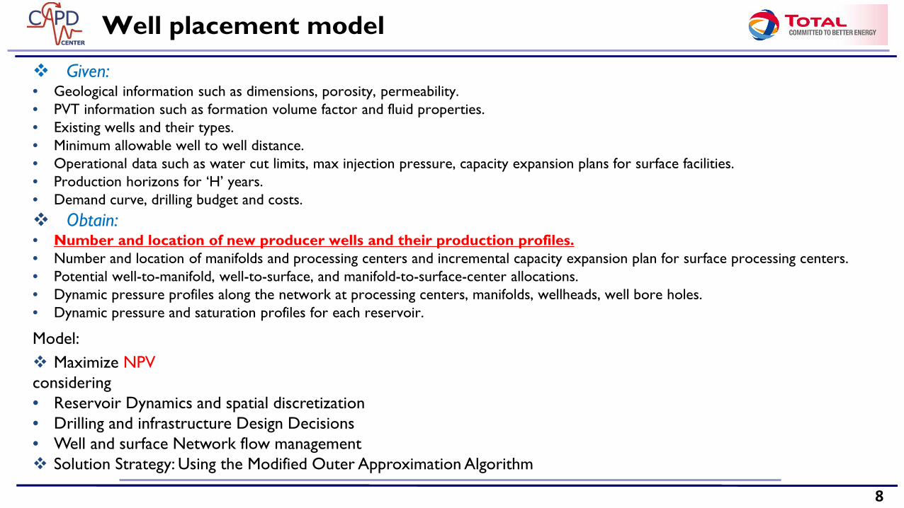
Well placement model

Given:• Geological information such as dimensions, porosity, permeability.• PVT information such as formation volume factor and fluid properties.• Existing wells and their types. • Minimum allowable well to well distance. • Operational data such as water cut limits, max injection pressure, capacity expansion plans for surface facilities. • Production horizons for ‘H’ years. • Demand curve, drilling budget and costs. Obtain:• Number and location of new producer wells and their production profiles. • Number and location of manifolds and processing centers and incremental capacity expansion plan for surface processing centers. • Potential well-to-manifold, well-to-surface, and manifold-to-surface-center allocations.• Dynamic pressure profiles along the network at processing centers, manifolds, wellheads, well bore holes. • Dynamic pressure and saturation profiles for each reservoir.

Model: Maximize NPVconsidering • Reservoir Dynamics and spatial discretization• Drilling and infrastructure Design Decisions• Well and surface Network flow management Solution Strategy: Using the Modified Outer Approximation Algorithm

8

The Mass Balances Equation

2-D discretization of reservoir

• Binary variable : y(n) 1 if a well should exist in cell ’n’

• Empirical equations for estimating BHP.

• Allow upstream mobility values for convective flows to be chosen dynamically based on pressure time map at time (t-1).

9

N1 N2 N3 N4

N5 N6 N7 N8

N9 N10 N11 N12

N13 N14 N15 N16

Dynamic multiphase flow in a reservoir

Backward finite difference approximation

STRATEGY : Bi-Level Decomposition

LOWER LEVELPLANNING PROBLEM

(PP)

no

Feasible?yes

Upper boundUB = ZDP

STOP no

Add integer cut

yes Lower boundLB = ZPP

UB - LB <Tolerance ?

yesSTOP

Solution is ZPP

Add design cuts Add integer cuts

no

UPPER LEVELDESIGN PROBLEM

( DP )Max NPV

Feasible?

DP : Vijay Gupta and Grossmann

(2012)

PP : Tavallali, Karimi et al.

(2012)

GRID BASED

10

Assignment of platformsto wells and their installation

Selection of wells and production planning

Incorporating field data

11

Two-level Optimization approach

• Upper level minimization of error (with data)min φ(u,v,Θ)s.t. max NPV(u,v,Θ) Lower level maximization NPV

s.t. g(u,v,Θ) ≤ 0Fitting error φ(Θ) = ½(u-u α)

₂

select Θ to minimize the error function.

• Lower level optimization of model (as shown in previous slide)

This approach ensures that we are not compromising on the number of degrees of freedom.

Conclusion and Future work

12

Model development for Production planning:

• Add Gas lift operations to the model.

Well placement model:

• Implementation of an improved optimization approach in the well placement model.

• Validation of the results from historical production data and ECLIPSE simulation.

• Integration of PETEX suite for well simulations.