integration of in situ imaging and chord length … of in situ imaging and chord length distribution...

Integration of in situ Imaging and Chord Length Distribution

Measurements for Estimation of Particle Size and Shape

Okpeafoh S. Agimelena,∗, Anna Jawor-Baczynskaa, John McGintya, ChristosTachtatzisb, Jerzy Dziewierzc, Ian Haleyd, Jan Sefcika, Anthony J. Mulhollande,∗

aEPSRC Centre for Innovative Manufacturing in Continuous Manufacturing and Crystallisation,Department of Chemical and Process Engineering, University of Strathclyde, James Weir Building,

75 Montrose Street, Glasgow, G1 1XJ, United Kingdom.bCentre for Intelligent Dynamic Communications, Department of Electronic and Electrical

Engineering, University Of Strathclyde, Royal College Building, 204 George Street, Glasgow, G11XW, United Kingdom.

cThe Centre for Ultrasonic Engineering, Department of Electronic and Electrical Engineering,University Of Strathclyde, Royal College Building, 204 George Street, Glasgow, G1 1XW, United

Kingdom.dMettler-Toledo Ltd., 64 Boston Road, Beaumont Leys Leicester, LE4 1AW, United KingdomeDepartment of Mathematics and Statistics, University of Strathclyde, Livingstone Tower, 26

Richmond Street, Glasgow G1 1XH, United Kingdom

Abstract

Efficient processing of particulate products across various manufacturing steps re-quires that particles possess desired attributes such as size and shape. Controlling theparticle production process to obtain required attributes will be greatly facilitated us-ing robust algorithms providing the size and shape information of the particles fromin situ measurements. However, obtaining particle size and shape information in situduring manufacturing has been a big challenge. This is because the problem of estimat-ing particle size and shape (aspect ratio) from signals provided by in-line measuringtools is often ill posed, and therefore it calls for appropriate constraints to be imposedon the problem. One way to constrain uncertainty in estimation of particle size andshape from in-line measurements is to combine data from different measurements suchas chord length distribution (CLD) and imaging. This paper presents two differentmethods for combining imaging and CLD data obtained with in-line tools in order toget reliable estimates of particle size distribution and aspect ratio, where the imagingdata is used to constrain the search space for an aspect ratio from the CLD data.

Keywords: Chord Length Distribution, Particle Size Distribution, Particle Shape,Focused Beam Reflectance Measurement, Imaging.

∗Corresponding authorsEmail addresses: [email protected] (Okpeafoh S. Agimelen),

[email protected] (Anthony J. Mulholland)

Preprint submitted to Chemical Engineering Science April 30, 2018

arX

iv:1

505.

0332

0v2

[ph

ysic

s.da

ta-a

n] 7

Jan

201

6

1. Introduction

One of key steps in the manufacture of particulate products in the pharmaceuticalsand fine chemicals industry is crystallisation, which is widely used for separation andpurification of intermediates, fine chemicals and active pharmaceutical ingredients. Thecrystals come in different sizes and shapes. Subsequent steps in the manufacturingprocess, such as filtration, drying, blending and formulation of final products, requirethat the particle sizes and shapes lie within some desirable range. In order to providemonitoring and control of crystallisation processes it is necessary to develop techniquesfor estimating the shape and size distribution of particles in situ. There are a numberof off line tools [1] that can be used to estimate the particle size distribution1 (PSD)of crystals produced in a crystallisation process. However, of particular importance tothe control of a crystallisation process are tools that can be used in situ. These toolsshould be suitable for estimating size and shape information of particles dispersed ina slurry without the need for sampling and/or dilution. Examples of such instrumentsare the focused beam reflectance measurement (FBRM), the three dimensional opticalreflectance (3D-ORM) [2] and the particle vision and measurement (PVM) [3] sensors.

In-line sensors such as FBRM and 3D-ORM measure a chord length distribution(CLD)2 which is related to the size and shape of the particles in a slurry. It has beena long standing challenge to be able to deduce the actual PSD and particle shape fromexperimental CLD data. In order to do this, an inverse problem needs to be solved. Thisis usually achieved by suitably discretising both CLD (which is already measured asa discrete distribution) and PSD and then constructing an appropriate transformationmatrix relating these two distributions [4–6]. The transformation matrix depends onthe choice of size bins used to discretise the two distributions and the correspondingsize ranges as well as the shape of particles. The transformation matrix is usuallynot known in advance and needs to be estimated along with the corresponding PSD(discretised) so that the convolution of the transformation matrix with the PSD yieldsa CLD which agrees with the experimentally measured CLD. However, this problemis ill posed. There are a number of different transformation matrices and PSDs whoseconvolutions give rise to the same CLD. Hence the challenge is how to estimate acombination of transformation matrix and PSD whose convolution will agree with anexperimentally measured CLD for a given slurry as well as the PSD estimated beingphysically reasonable and representative of the particles in the slurry.

The approach which was used in previous works [7–10] when estimating the trans-formation matrix was to assume the same shape (quantified by a metric referred to asaspect ratio) for all the particles in the slurry, and then use a previously estimated3

1The term particle size distribution is broadly used here to refer both to continuous analyticalprobability density functions for particle sizes and discretised probability histograms of the particlesizes.

2Similar to the case of PSD, the term chord length distribution is used to cover both continuousanalytical functions and discretised probability histograms.

3The approach was to estimate the range of particle sizes in a sample by techniques such as sieving,

2

range of particle sizes in the slurry to construct the transformation matrix. This ap-proach is not suitable for monitoring a crystallisation process where nucleation and/orgrowth of particles was present as neither the range of particle sizes nor their aspectratio would be known in advance. A technique which was suitable for estimating therange of particle sizes in a slurry in situ was presented in our previous work [6]. How-ever, like in other previous works, the transformation matrix was constructed with asingle aspect ratio for all particles. This leaves open a possibility that the transforma-tion matrix is constructed with inappropriate aspect ratio or that there is a wider rangeof aspect ratios present for particles of same or different sizes. It was demonstrated inour previous work [6] that it was still possible to calculate different CLDs that all hada very good agreement with an experimentally measured CLD even though some of thetransformation matrices were constructed at aspect ratios that were far from the shapeof the particles described. However, it was also shown that as the aspect ratio deviatedfurther from the true shape of the particles, then the corresponding PSD became in-creasingly noisy. This situation led to the introduction of a penalty function in order toeliminate unrealistic aspect ratios. However, when there is a wide variation of aspectratios of the particles in the slurry, there is a need to introduce further constraints onthe aspect ratio to reduce the search space and regularize the inverse problem. Oneway to do this is to get estimates of aspect ratio (within some reasonable bounds) usingimaging, and then use this information to constrain the search for a representative as-pect ratio. However, the imaging needs to be done in situ in order to develop techniquesfor estimation of PSD and particle shape which could be used for real time monitoringand control of particle production processes.

While it would be desirable to get good estimates of both PSD and particle aspectratio using in situ imaging alone, this is currently not the case. The currently availablein-line imaging tools (for example, the PVM used in this work) produce 2D projectionimages. Furthermore, the objects in the images may be partially or completely out offocus, parts of imaged object may cross the image frame or objects may overlap eachother4. Although advanced measurement equipment have been developed which can beused to capture 3D images of particles in a slurry and make good estimates of PSD andshape of particles, it requires sampling and dilution flow loops5 to allow capturing 3Dimages of individual particles in a flow-through cell [11–14]. Therefore this approachmay not be generally applicable for in-line monitoring of particle manufacturing pro-cesses. Hence the current situation is that PSD cannot be estimated to a good degreeof accuracy using routinely available in-line imaging tools. To overcome this challenge,we propose to combine in-line CLD measurements with imaging data to provide morereliable estimate of quantitative particle attributes.

laser diffraction, microscopy or use information supplied by the manufacturer before suspending theparticles.

4The issue of objects overlapping each other would not be a problem if an appropriate imageprocessing algorithm which can resolve the objects is used.

5The dilution is necessary to avoid instances of overlapping particles in images.

3

In this paper, we present two different methods for combining imaging data withCLD data for particle size and shape estimation. The first method presented herecalculates an estimate of the mean aspect ratio of all the particles in the slurry andthen uses this information to constrain the search space for size and shape estimationfrom the CLD data. In the second method, a distribution of aspect ratios for eachparticle size is used for the PSD estimation. The distribution of aspect ratios is basedon the data from the captured images.

2. Experiment

To demonstrate the technique for estimating particle size and shape informationusing a combination of the CLD and imaging data, experiments were performed inslurries containing particles of different shapes. The materials and procedure are de-scribed below.

2.1. Materials

Three different samples were used for the measurements. Sample 1 consisted ofpolystyrene (PS) microspheres purchased from EPRUI nanoparticles and MicrospheresCo. Ltd. with batch number 2012-5-7, and 0.2g of the PS microspheres were dispersedin 100g of isopropanol (IPA) purchased from VWR (20842.323) giving a concentra-tion of 0.2% by weight. Sample 2 consisted of cellobiose octaacetate (COA) particlesobtained from GSK. The particles were dispersed in methanol (purchased from VWR(20847.307)) with the same concentration as in sample 1. Sample 3 consisted of glycine(Glycine) crystals obtained by cooling crystallisation from an aqueous solution. Thesolution with glycine concentration of 340mg/ml was prepared using glycine (purchasedfrom Sigma-Aldrich (G8898, ≥ 99% TLC)) and deionized water (from an in-house Mil-lipore Water System (18MΩ/cm)). The solution was cooled from a temperature of90C to a temperature of 43C at a rate of 3C/min. During this process the glycinecrystallised out of solution until an equilibrium particle size distribution was reached.The crystallisation of glycine was monitored with the FBRM probe which showed aninitial increase (in time) of chord lengths before eventually reaching a steady state.

2.2. Experimental Setup

The suspension of particles for all samples was made in the Mettler Toledo EasyMax102 system. The EasyMax system consists of a cylindrical jacketed vessel of volume100ml with different stirrer and blade options. An anchored overhead stirrer withpitched (45 pitch angle) blades was used in all the experiments in this work. Thestirrer shaft and probes were inserted into the slurries through ports located at the topof the set up. The stirring speed was set at 400 rpm in all experiments.

The CLD measurements were made with a Mettler Toledo FBRM G400 probe. Theimages of the particles were captured with a Mettler Toledo PVM V819 probe duringthe period of CLD measurement. The FBRM sensor consists of a system of lenses whichfocus a laser beam onto a spot near the probe window in the slurry. The laser spot

4

Chord length (µm)100 101 102 103

Counts

0

20

40

60


Counts

0

50

100

Chord length(µm)100 101 102 103

Counts

0

100

200(a)

PS

(b)

(c)

Glycine

COA

Figure 1: The CLD (measured with the FBRM G400 sensor) for the (a) PS, (b) COA and (C) Glycinesamples.

moves in a circular trajectory and the back scattered light is detected. The chord lengthis then calculated as the speed of the laser spot multiplied by the duration of the backscattered light as the laser traverses a particle. The FBRM sensor records the lengthsof the chords for a pre-set duration after which the CLD is reported [2, 6, 15–17].

The PVM is an in situ microscope which consists of eight laser sources enclosed ina cylindrical tube. The six forward lasers and two back lasers (achieved by reflectingtwo lasers off a Teflon cap at the probe window) illuminate the particles in the slurry.The back scattered light is detected by a CCD element from which grayscale images areconstructed. The image frame of the CCD array consists of 1360×1024 pixels with apixel size of 0.8µm. The PVM V819 sensor has a maximum acquisition rate of 5 imagesper second, although lower rates of acquisition could be set depending on requirements.The depth of the focal zone is restricted to about 50µm so that all objects that are infocus result in images that have identical magnification levels. Each of the lasers canbe switched on or off so that different degrees of illumination can be achieved.

3. Experimental Data

The CLD data measured with the FBRM sensor for PS is shown in Fig. 1(a). Imageswere captured with the PVM sensor during the CLD measurement. A representativeimage from the PS sample is shown in Fig. 2(a).

Similarly, the CLD data recorded for COA is shown in Fig. 1(b) while that of

5

(a)

(b)

(c)

Figure 2: Representative images (obtained with the PVM V819 sensor) for the (a) PS, (b) COA and(c) Glycine samples. The images have the same width of 1088µm and height of 819µm.

Glycine is shown in Fig. 1(c). Representative images for COA and Glycine are shownin Figs. 2(b) and 2(c) respectively. A total of 600 images were acquired each for PSand COA, and 121 images for Glycine.

4. Image Analysis

As mentioned in the introductory section, an estimate of the PSD and particle shapecan be made from images alone without the need to include CLD data. However, due tothe reasons discussed in the introductory section, this approach is not always convenient.The techniques presented here utilise images obtained with an in-line measuring tool.However, due to the limitations in the images (as discussed in the introductory section),it is necessary to combine the imaging data with CLD to obtain reasonable aspect ratioand/or size estimates.

The images captured with the PVM are processed in order to detect the objectscontained in them and hence obtain information about the shape of the particles inthe slurry. However, the image processing algorithm used in this work does not havefeatures to resolve an object completely when it does not lie entirely in focal plane ofthe PVM sensor. Also, it does not have functionalities to resolve overlapping objects inimages. For this reason the samples used in this work were deliberately prepared dilute6

6Low slurry densities have been used here for the purpose of methods development. Future work willinvolve the investigation of the applicability of the methods developed here at higher slurry densities

6

to reduce instances of overlapping objects. The parameters7 of the image processingalgorithm were tuned to reject most of the particles that were not entirely in the focalplane of the PVM sensor. However, the imaging data still has some degree of inac-curacy as seen in the error bars of the data (see subsection 4.6 of the supplementaryinformation). This limitation not withstanding, the data from the images was suffi-ciently accurate to demonstrate the techniques developed in this work. Furthermore,images which do not contain objects that are contained completely within the imageframe were also discarded. This situation of having to discard some images reduces thenumber of data sets that can be gathered from the images. However, it can be shown(see section 2 of the supplementary information) that with a sample size (number ofobjects) of about 500 the error incurred in estimating the aspect ratio is reduced to areasonable extent. However, for a more robust estimate of the PSD using imaging data,a larger number of objects will be required. The number8 of detected objects used inthis work is just sufficient to demonstrate the methods developed here. The issue ofobjects not completely in focus can be dealt with if additional functionalities are addedto the image processing algorithm, but this is beyond the scope of this work. The keysteps for detecting objects in the images captured by the PVM sensor are summarisedin subsection 4.1.

4.1. Object Detection

The raw grayscale images from the PVM sensor are passed through a median filterto remove speck noise from the image background which is homogeneous. At this stageobjects on the boundary of the image frame are removed. Any object with surface areabelow 900 pixels9 is considered noise and excluded from processing. Finally, a closingoperation with a disk structural element is used to join broken edges. The resultingblob properties such as area, centroid, eccentricity, convex area, and major and minoraxes can be obtained. These steps are summarised in Fig. 3. The tunable parameters ofthe image processing algorithm are summarised in subsection 4.5 of the supplementaryinformation.

4.2. Characterising Particle Shape

The following procedure is used to obtain a shape descriptor, which is then used tocharacterise the shape of each particle. Each boundary pixel j of object i has coordinates

(with a more advanced image processing algorithm) using suspensions of particles of known PSD,then the degree of deviation of the results from the known PSD can be quantified at different slurrydensities.

7The parameters of the algorithm need to be tuned for different samples due to variation of contrast.8A total of 1393 objects were detected for PS, 1810 for COA and 526 for Glycine.9The surface area of 900 pixels represents length dimensions of approximately 30 × 30 pixels

(assuming a square geometry). This implies that objects that are smaller than approximately 24µmare rejected by the image processing algorithm. The consequence is that there is no estimate of aspectratio for these small objects. However, the particles used in this work have sizes mostly in the rangeof 100µm so that the effects of this are minimal.

7

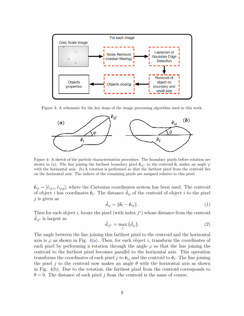
Figure 3: A schematic for the key steps of the image processing algorithm used in this work.

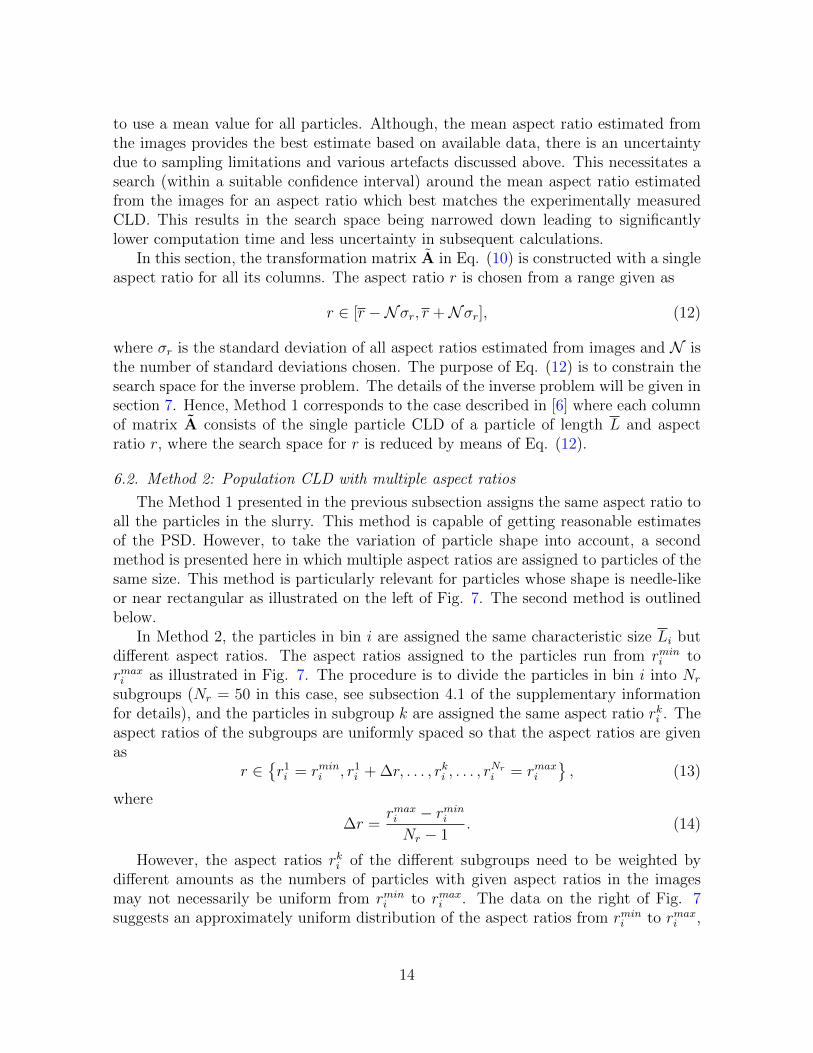
Figure 4: A sketch of the particle characterisation procedure. The boundary pixels before rotation areshown in (a). The line joining the farthest boundary pixel eij∗ to the centroid ei makes an angle ϕwith the horizontal axis. (b) A rotation is performed so that the farthest pixel from the centroid lieson the horizontal axis. The indices of the remaining pixels are assigned relative to this pixel.

eij = [eij,x, eij,y], where the Cartesian coordinates system has been used. The centroidof object i has coordinates ei. The distance dij of the centroid of object i to the pixelj is given as

dij = ‖ei − eij‖ . (1)

Then for each object i, locate the pixel (with index j∗) whose distance from the centroiddij∗ is largest as

dij∗ = maxjdij. (2)

The angle between the line joining this farthest pixel to the centroid and the horizontalaxis is ϕ as shown in Fig. 4(a). Then, for each object i, transform the coordinates ofeach pixel by performing a rotation through the angle ϕ so that the line joining thecentroid to the farthest pixel becomes parallel to the horizontal axis. This operationtransforms the coordinates of each pixel j to eij and the centroid to ei. The line joiningthe pixel j to the centroid now makes an angle θ with the horizontal axis as shownin Fig. 4(b). Due to the rotation, the farthest pixel from the centroid corresponds toθ = 0. The distance of each pixel j from the centroid is the same of course.

8

Angles (rads)0 2 4 6

Dista

nce(µm)

0

20

40

60

80

Lmin

Lmax


Dista

nce(µm)

0

20

40

60

80

L2min

L2max

L1max

L1min


Dista

nce(µm)

0

20

40

60

80

L1min L2min

L1max

L2max

(a)

COA

PS

(b) (c)

Glycine

Figure 5: The shape descriptor (d in Eq. (4)) as a function of the angle (θ) for the (a) PS, (b) COAand (c) Glycine samples.

Since the sample rate with respect to θ is not uniform, then the pixel distanceswere resampled with Np uniformly spaced θ values constructed as θp = p∆θ, ∆θ =2π/Np, p = 1, 2, . . . , Np. This allows the vector of all pixels distances (from thecentroid) for object i to be written as

di = [di1, di2, . . . , diNp ]. (3)

Finally, the average vector d of all pixel distances for all objects detected by the imageprocessing algorithm can be calculated as

d =1

Nobj

Nobj∑i=1

di, (4)

where Nobj is the number of objects detected from all the images analysed.A plot of d versus angle (θ) can be made as shown in Figs. 5(a) to 5(c). For near

spherical particles, the shape descriptor d is nearly constant as in the case of PS inFig. 5(a). However, for elongated particles, the shape descriptor d has two minimaand maxima as in the cases of CoA and Glycine in Figs. 5(b) and 5(c). The shapedescriptor shown in 5(a) to 5(c) is similar to the type described in [13].

In an ideal situation, the shape descriptor for spherical particles will be constantat a value representing the radius of the spherical particles. However, since the PSparticles are not perfectly spherical there is slight variation in the dimensions so that

9

an average aspect ratio r (the ratio of the minor to the major dimension) can beestimated. Similarly, the maxima in the shape descriptors for the CoA and Glycineparticles (in Figs. 5(b) and 5(c)) represent the major dimension of the particles whilethe minima represent the minor dimension of the particles.

For the case of the PS particles the mean aspect ratio r is estimated from theminimum dimension Lmin and maximum dimension Lmax (see Fig. 5(a)) as

r =LminLmax

. (5)

In the case of elongated particles, the maximum dimension (average length of particles)is given as Lmax = L1max + L2max (shown in Figs. 5(b) and 5(c)) and the minimumdimension (average width of particles) is given as Lmin = L1min + L2min. So that theaverage aspect ratio can then be estimated using Eq. (5).

However, the aspect ratios for individual particles will be different from r. Theaspect ratio for each particle is estimated from the shape descriptor correspondingto that particle. Once the aspect ratios of individual particles are estimated, then ascatter plot of aspect ratio versus particle length can be made as shown in Figs. 6(a)to 6(c). The shape descriptors for individual particles are not always smooth as inthe cases shown in Figs. 5(a) to 5(c). They contain different degrees of variation dueto imperfections in the particles and images (see subsection 4.6 of the supplementaryinformation for details).

Furthermore, the aspect ratios estimated from the shape descriptor for individualparticles contain some artefacts (as can be seen in Fig. 6) due to a number of factors.These factors include deformations in the particles (that is, particles whose shapesdeviate from the majority of particles in the slurry), impurity objects in the monitoredslurry and particles not completely in focus10. For example, aspect ratios as low asabout 0.2 in the case of the spherical particles in Fig. 6(a) or the minor peak at aspectratio r ≈ 0.5 in Fig. 6(d) are artefacts.

Figures 6(b) and 6(c) suggest the presence of particles of sizes up to about 500µmin the COA and Glycine samples respectively. However, the number of data points (inFigs. 6(b) and 6(c)) corresponding to these large particles may not be representativeof the actual number of these large particles in the slurry. This is because the imageprocessing algorithm has been designed to remove objects making contact with theimage frame, and larger particles have a higher probability of making contact withthe image frame. In the situation where the PSD is to be estimated from image dataalone, then this probability will need to be taken into account [18]. However, since theobjective here is just to estimate the aspect ratio of particles of different sizes, then thisis not a crucial issue.

10The image processing algorithm parameters are tuned to remove particles that are out of focus.However, when the particle is only partially in focus, the image processing algorithm detects only partof the particle and this leads to an error in the estimated aspect ratio for that particle.

10

Particle length (µm)0 200 400

Aspectratio

0

0.2

0.4

0.6

0.8

Aspect ratio0 0.5 1

Frequency

0

50

100

Particle length(µm)50 100 150

Aspectratio

0.2

0.4

0.6

0.8

Aspect ratio0 0.5 1

Frequency

0

200

400

600

Particle length(µm)0 200 400

Aspectratio

0

0.2

0.4

0.6

Aspect ratio0 0.5 1

Frequency

0

100

200

PS

COA

Glycine

(d) (e)

(a) (b) (c)

PS COA

(f)

Glycine

Figure 6: Scatter plots of the aspect ratio versus particle length for individual objects for (a) PS,(b) COA and (c) Glycine. The histograms of the aspect ratios are shown in (d) PS, (e) COA and(f) Glycine.

The histogram (in Fig. 6(d))11 for the spherical particles has a dominant mode closeto the aspect ratio of 0.85 which is close to the average aspect ratio r ≈ 0.8 estimatedfrom the average shape descriptor (in Fig. 5(a)) for this slurry. Similarly the modes ofthe histograms (in Figs. 6(e) and 6(f)) for COA and Glycine occur close to aspect ratiosof 0.2 and 0.4 respectively. These values are close to the average aspect ratios r ≈ 0.2(for COA) and r ≈ 0.4 (for Glycine) obtained from their respective shape descriptorsin Figs. 5(b) and 5(c).

5. Modelling Chord Length Distribution

The sizes of particles in a slurry can be represented by the equivalent sphericaldiameter as was done in [6]. However, a characteristic length L could also be used,which can be chosen as the distance between the two extreme points in the particles’geometry. Since the estimated sizes from the images is L, then this metric is used herefor consistency with the image data. Once the metric for particle sizes has been chosen,then the PSD can then be expressed in terms of the chosen particle size metric. The

11The uniform bin widths of the histograms in Figs. 6(d) to 6(f) were estimated using the Freedman-Diaconis rule [19]. The number of bins were then estimated as 18 bins for PS, 28 bins for COA and13 bins for Glycine.

11

PSD X is related to the CLD C by means of a convolution function [2, 6, 20] and therelationship can be written in matrix form as [6] 12

C(s) = A(s, L)X(L), (6)

where s is the chord length, and X is the length weighted PSD [6] given as

Xi = LiXi, i = 1, 2, 3, . . . , N. (7)

The PSD Xi (which is actually a histogram) consists of N bins. The characteristic sizeLi of particle size bin i is the geometric mean of sizes Li and Li+1 as Li =

√LiLi+1.

The bin boundaries are calculated as

Li = Lminωi−1, i = 1, 2, . . . , N + 1 (8)

where

ω =

(LmaxLmin

) 1N

, (9)

where Lmin is the left boundary of the first particle size bin and Lmax is the rightboundary of the last particle size bin.

In previous works [7–9, 21–23] the values of Lmin and Lmax were estimated fromsuitable measurements. However, the technique of estimating Lmin and Lmax directlyfrom the bin boundaries of the CLD histogram using a moving window technique hasbeen demonstrated to yield more accurate results [6]. This window technique is moresuitable for estimating the sizes of particles in-line in a process where particle sizeinformation is obtained from the CLD [6].

The length weighting applied to the PSD X in Eq. (7) is necessary because the CLDfor a population of particles is biased towards particles of larger sizes [6, 20, 24, 25]. Theforward problem in Eq. (6) is implemented by considering a chord length histogram Cjof M bins where the characteristic chord length sj of bin j is the geometric mean ofthe chord lengths of sj and sj+1 as outlined in [5, 6].

If the PSD for a population of particles is known, then the CLD can be calculatedusing Eq. (6). However, in practical situations, the particle size histogram Xi is notknown in advance resulting in the inverse problem of calculating an unknown PSD Xi

from a known CLD Cj. For this reason, the forward problem in Eq. (6) is reformulatedas

C(s) = A(s, L)X(L), (10)

where the matrix A is obtained from matrix A by multiplying each column of A bythe corresponding particle length as described in [6].

12Note that the symbol L was used to represent the length of a chord in [6]. However, the symbolL is used to represent the characteristic length and s the length of a chord in this work. The CLDC and PSD X in Eq. (2) have been discretised. As such they are not continuous probability densityfunctions and the term distribution is used in this work for simplicity.

12

Each column i of matrix Aji is calculated from the CLD of a single particle (singleparticle CLD) of length Li and given aspect ratio ri. In the current work, the singleparticle CLD used in constructing the columns of matrix A are obtained from theanalytical Li and Wilkinson (LW) model [5]13.

The process of calculating the single particle CLD involves computing the relativelikelihood of obtaining a chord of length s from a particle of a given length and aspectratio [5]. The LW model gives a probability density function (PDF) which can beused in making this calculation for ellipsoidal shaped particles14. The PDF is derivedfrom an ellipsoid of semi major axis length a, semi minor axis length b and aspect ratior = b/a [5]. The LW model gives the probability pLi

(sj, sj+1) of obtaining a chord whose

length lies between sj and sj+1 from an ellipsoid of characteristic length Li = 2ai (seesection 1 of the supplementary information and [5, 6] for the mathematical expressionfor pLi

(sj, sj+1)). Once the probabilities are calculated, then for each row j of matrixA the columns are constructed as

Aj =[pL1

(sj, sj+1), pL2(sj, sj+1), . . . , pLi

(sj, sj+1), . . . , pLN(sj, sj+1)

]. (11)

6. Incorporating aspect ratio from images

As stated in section 5 the calculation of a column of matrix A requires the charac-teristic size of the particle size bin corresponding to that column, as well as the aspectratio r of the particle of that characteristic size. In the previous work [6], all parti-cles were assumed to have the same aspect ratio, and its value was estimated using analgorithm based solely on CLD data. The single aspect ratio approach will be usedin subsection 6.1, where the single aspect ratio value is estimated from imaging data.This approach is most suitable for the case of spherical particles where the aspect ra-tios of the individual particles are tightly packed around some mean value. However,for the case of particles where there is a wider spread of aspect ratios, a variation ofaspect ratios for different particle sizes can also be used. The corresponding techniqueis outlined in subsection 6.2.

6.1. Method 1: Population CLD with a single aspect ratio

When the aspect ratios are tightly packed around some mean value as in the caseof spherical (or near spherical) particles in Figs. 6(a) and 6(d), it may be desirable

13Even though the model by Vaccaro et al. [25] gave estimates of particle aspect ratios that werecloser to the estimates from images in [6], the LW model is used in this work for the CLD calculation.The reason is that the Vaccaro model is restricted to small values of aspect ratios r . 0.4, whereas theimage data in Fig. 3 cover aspect ratios of r ≈ 0.1 to r ≈ 0.9. The LW model covers the entire rangefrom r = 0 to r = 1.

14The shapes of the COA and Glycine particles in this work have been approximated as ellipsoids.However, this is only an approximation as Fig. 2(c) clearly shows that the Glycine particles arefaceted. The use of ellipsoids to represent faceted objects introduces some discrepancy between thesingle particle CLDs of both objects (see section 8 of the supplementary information for details).However, the ellipsoid approximation used here is sufficient to illustrate the methods presented here.

13

to use a mean value for all particles. Although, the mean aspect ratio estimated fromthe images provides the best estimate based on available data, there is an uncertaintydue to sampling limitations and various artefacts discussed above. This necessitates asearch (within a suitable confidence interval) around the mean aspect ratio estimatedfrom the images for an aspect ratio which best matches the experimentally measuredCLD. This results in the search space being narrowed down leading to significantlylower computation time and less uncertainty in subsequent calculations.

In this section, the transformation matrix A in Eq. (10) is constructed with a singleaspect ratio for all its columns. The aspect ratio r is chosen from a range given as

r ∈ [r −Nσr, r +Nσr], (12)

where σr is the standard deviation of all aspect ratios estimated from images and N isthe number of standard deviations chosen. The purpose of Eq. (12) is to constrain thesearch space for the inverse problem. The details of the inverse problem will be given insection 7. Hence, Method 1 corresponds to the case described in [6] where each columnof matrix A consists of the single particle CLD of a particle of length L and aspectratio r, where the search space for r is reduced by means of Eq. (12).

6.2. Method 2: Population CLD with multiple aspect ratios

The Method 1 presented in the previous subsection assigns the same aspect ratio toall the particles in the slurry. This method is capable of getting reasonable estimatesof the PSD. However, to take the variation of particle shape into account, a secondmethod is presented here in which multiple aspect ratios are assigned to particles of thesame size. This method is particularly relevant for particles whose shape is needle-likeor near rectangular as illustrated on the left of Fig. 7. The second method is outlinedbelow.

In Method 2, the particles in bin i are assigned the same characteristic size Li butdifferent aspect ratios. The aspect ratios assigned to the particles run from rmini tormaxi as illustrated in Fig. 7. The procedure is to divide the particles in bin i into Nr

subgroups (Nr = 50 in this case, see subsection 4.1 of the supplementary informationfor details), and the particles in subgroup k are assigned the same aspect ratio rki . Theaspect ratios of the subgroups are uniformly spaced so that the aspect ratios are givenas

r ∈r1i = rmini , r1i + ∆r, . . . , rki , . . . , r

Nri = rmaxi

, (13)

where

∆r =rmaxi − rmini

Nr − 1. (14)

However, the aspect ratios rki of the different subgroups need to be weighted bydifferent amounts as the numbers of particles with given aspect ratios in the imagesmay not necessarily be uniform from rmini to rmaxi . The data on the right of Fig. 7suggests an approximately uniform distribution of the aspect ratios from rmini to rmaxi ,

14

Particle length (µm)0 100 200 300 400 500

Aspectratio

0

0.2

0.4

0.6

0.8

rmaxi

rmini

Li

Li+1

Li

Figure 7: Left: A schematic to illustrate the assignment of different aspect ratios to particles of thesame length. Right: A scatter plot to illustrate the maximum aspect ratio rmax

i and minimum aspectratio rmin

i for a particular bin i for calculating the columns (of slice i) of the 3 D matrix in Eq. (15).

hence the aspect ratios were assigned to each of the subgroup k with equal weight inthis case.

Once aspect ratios have been assigned to different particle size bins15, then a 3Dprobability array Ajki is constructed. Each slice i of the array corresponds to a par-ticle of size Li, and each column k of slice i contains the probabilities p

Lki(sj, sj+1) of

obtaining chords whose lengths lie between sj and sj+1 from a particle of size Li andaspect ratio rki . Hence the 3D array consists of M rows, Nr columns and N slices. Thetransformation matrix Aji in Eq. (10) is then obtained from the 3D array by averagingover the slices as

Aji =1

Nr

Nr∑k=1

Ajki. (15)

This simple averaging is carried out since the aspect ratios rki are assigned to thesubgroups k with equal weights. This is the simplest way to construct the matrix Ajifrom the 3D array Ajki, and this approach is supported by the data from the images asshown on the right of Fig. 7. It is possible to introduce a probability distribution for theaspect ratios assigned to the subgroups, but this simple approach has been used herefor the purpose of illustrating the technique. Once the matrix Aji has been constructed,then the forward problem in Eq. (10) can be solved for a given PSD Xi.

15Details of the technique for combining the aspect ratios with the windowing technique developedin [6] can be found in section 5 of the supplementary information.

15

7. PSD Estimation

As mentioned in section 5, the problem encountered in practical situations is theestimation of the PSD Xi corresponding to an experimentally measured CLD C∗j . Thisis the inverse problem to the forward problem given in Eq. (10). One of the key steps inthe process of the PSD estimation is to determine the transformation matrix A in Eq.(10) as accurately as possible. The level of accuracy of the matrix A depends on thevalues of Lmin and Lmax as well as the aspect ratio(s) used in calculating its columns.

To determine the best possible values of Lmin and Lmax, the forward problem in Eq.(10) is rewritten as

C = AX + ε, (16)

where ε is an additive error between the calculated and experimentally measured CLD.Then for given values of Lmin, Lmax, values of the fitting parameter γ are found16 whichminimises the objective function f1 given as

f1 =M∑j=1

[C∗j −

N∑i=1

AjiXi

]2, (17)

whereXi = eγi , i = 1, 2, 3, . . . , N. (18)

A trial solution of γi = 0 was used in the calculation of the vector Xi from Eq. (17).Once the solution vector Xi is obtained, then it is used to solve the forward problemin Eq. (10) to obtain a calculated CLD Cj, j = 1, 2, . . . ,M , where M is the number ofbins in the CLD histogram17. The procedure is repeated until the optimum values ofLmin and Lmax are found for which there is the best match between the calculated andexperimentally measured CLD.

The objective function f1 given in Eq. (17) is suitable for estimating the optimumvalues of Lmin and Lmax whether the same aspect ratio is assigned to all particles or adistribution of aspect ratios is assigned to particles of the same size. In the case wherea single aspect ratio is assigned to all particles, the objective function f1 is not suitablefor picking out the best aspect ratio within the confidence interval of aspect ratios. This

16The Levenberg-Marquardt (LM) algorithm as implemented in Matlab was used in this work tosolve the optimisation problem here. The PSD Xi is estimated by means of the parameter γi. Aninitial value of γi is passed on to the LM algorithm which then searches for the optimum value of γito fit the given CLD. Since the PSD Xi is defined as an exponential function in Eq. 18, then theparameter γi can take values in the interval (−∞,+∞) and still give Xi ≥ 0. This implies that thenon negativity requirement on the PSD is maintained by the formulation of Xi in Eq. 18. Thereforethe LM algorithm was run without the use of lower or upper bounds as the parameter γi is defined in(−∞,+∞).

17The value of M = 100 was used in all the calculations here to mimic the number of bins set in theFBRM G400 sensor. The values of N = 70 and N = 50 were used in Methods 1 and 2 respectively.See subsection 4.2 of the supplementary information for more details on the choice of the values of Nfor the two methods.

16

task is accomplished with another objective function f2 (to be introduced in subsection7.1). The calculation for estimating the best aspect ratio (within the confidence intervalof aspect ratios) using the objective function f2 is carried out with the values of Lminand Lmax estimated with the objective function f1. However, in the other case wherea distribution of aspect ratios is assigned to particles of the same size, the objectivefunction f2 is not used as the problem of determining the best aspect ratio has beenremoved.

Once the optimum values of Lmin and Lmax and (in the case of Method 1) the bestaspect ratio have been estimated, then the PSDs (both number and volume based)can be calculated. However, these PSDs may not be reasonably smooth, showing non-physical oscillations as is often the case when solving ill-posed problems. In such cases,a third objective function f3 (to be introduced in subsection 7.3) is used to calculatesmooth PSDs. The calculation is carried out using the optimum values of Lmin and Lmaxobtained with the objective function f1 and in the case of Method 1, the best aspectratio obtained with the objective function f2. The calculation of the smooth PSDs withthe objective function f3 is done using suitable criteria described in subsection 4.4 ofthe supplementary information.

As stated above, the objective function f1 is used to obtain the optimum values ofLmin and Lmax for both Methods 1 and 2. A given pair of Lmin and Lmax are said tobe optimum when the corresponding calculated CLD C has the best match with theexperimentally measured CLD C∗. The level of agreement between the calculated andexperimentally measured CLD is assessed by computing the L2 norm

‖C∗ −C‖ =√f1. (19)

The values of Lmin and Lmax for which the L2 norm in Eq. (19) reaches a minimumare chosen as the optimum values.

7.1. PSD estimation for Method 1

In Method 1 the search for the optimum values of Lmin and Lmax using the objectivefunction f1 is done at each aspect ratio within the confidence interval in Eq. (12).However, for particles of a given shape, the L2 norm in Eq. (19) initially decreases withincreasing aspect ratio and then becomes level (see subsection 4.3 of the supplementaryinformation for details). This leads to non-uniqueness in determining the optimumvalue of r [6]. This problem of non-uniqueness is removed by using a modified objectivefunction f2 which contains a penalty term to control the size of the calculated PSDvector as

f2 =M∑j=1

[C∗j −

N∑i=1

AjiXi

]2+ λ1

N∑i=1

X2i , (20)

where the parameter λ1 sets the level of imposed penalty. The value of λ1 is chosenby comparing the magnitudes of the terms in Eq. (20) (see subsection 4.3 of thesupplementary information). The aspect ratio at which the objective function f2 reachesa minimum is then chosen as the optimum.

17

The solution vector (which is a number based PSD) obtained from Eq. (20) is notnecessarily smooth as the penalty imposed on the solution vector only restricts its mag-nitude. With this penalty function, the LM algorithm could settle on a solution vectorthat contains some local fluctuations but whose value of f2 is slightly less than a nearbysolution that is smooth. For this reason, a new objective function f3 (see subsection7.3 for details) which contains a penalty term to control the second derivative (to im-prove the smoothness of the solution vector) of the solution vector is used to estimate anumber based PSD whose corresponding CLD is compared with the experimental data.

7.2. PSD estimation for Method 2

In Method 2 (described in subsection 6.2) particles of different characteristic sizesLi are assigned a range of aspect ratios as outlined in subsection 6.2. This eliminatesthe need to search for the best global aspect ratio which is the situation in Method 1.Hence in Method 2, it is only necessary to search for the best values of Lmin and Lmaxusing the objective function f1. Once the optimum transformation matrix is obtainedusing the objective function f1, then the corresponding smoothed solution is obtainedwith the objective function f3 (given in Eq. (21)).

7.3. Volume based PSD

It is often necessary to recast the PSD Xi (which is number based) in Eq. (17)as a volume based PSD since most instruments for measuring PSD give the data interms of a volume based PSD. A new technique which allows suitable penalties to beimposed on the calculated volume based PSD Xv was introduced in [6]. In the currentwork, a smoothing penalty (referred to in subsection 7.1, see also [26]) is imposed. Thisis because the estimated volume based PSD Xv may contain significant non-physicaloscillations even though the corresponding number based PSD only contains none orminor fluctuations. The objective function f3 (see Eq. (21)) used to impose smoothnesson the volume based PSD can also be used to obtain a smooth number based PSD.Hence the function f3 is given in Eq. (21) in terms of generic quantities depending onwhether the number based or volume based PSD is being computed.

The function f3 is given as

f3 =M∑j=1

[C+j −

N∑i=1

A+jiX

+i

]2+ λ2

N∑i=1

[∇2h

[X+i

]]2. (21)

In the case of a number based PSD, the CLD C+j = C∗j (the experimentally measured

CLD), the matrix A+ji = Aji

18, and the solution vector X+i = Xi. However, in the

18The matrix Aij is the transformation matrix in the forward problem in Eq. (10) initially estimatedwith the objective function f1 in Eq. (17). The smoothed solution is then calculated using the functionf3 in Eq. (21) at a unique aspect ratio determined using the function f2 in Eq. (20). The solutionvector Xi from Eq. (17) is used to construct a trial solution as γi = ln(Xi) in the case of the numberbased PSD. For the volume based PSD, the corresponding number based PSD from Eq. (21) is usedto construct a trial solution as described in section 3 of the supplementary information.

18

case of the volume based PSD, the vector X+i = Xv

i (in the case where smoothing isnot required19, then the volume based PSD Xv

i is obtained from an objective functionsimilar to f1 in Eq. (17) as described in section 3 of the supplementary information,otherwise Eq. (21) is used), the matrix A+

ji will be scaled accordingly (see section

3 of the supplementary information for details), and the vector C+j = C∗ where the

transformed CLD C∗ is calculated as

C∗j =N∑i=1

AjiXi, (22)

where

Xi =Xi∑Ni=1Xi

. (23)

The operator ∇2h is a finite difference approximation to the second derivative of the

vector X+i given as [27]20

∇2h =

h−X+i+1 − (h+ + h−)X+

i + h+X+i−1

12h+h−(h+ + h−)

, (24)

where

h− = Li − Li−1h+ = Li+1 − Li (25)

and X+i has been treated as a function of the characteristic particle size L. The pa-

rameter λ2 sets the level of penalty imposed on the second derivative of X+i . If the

value of λ2 is sufficiently large, then the penalty on the second derivative causes the LMalgorithm to search for a solution vector which is smooth thereby avoiding solutionswith localised oscillations (see subsection 4.4 of the supplementary information).

The volume based PSD obtained from Eq. (21) is normalised and converted to aprobability density distribution as

Xvi =

Xv

i

(Li+1 − Li)∑N

i=1Xv

i

. (26)

8. Results and Discussion

The results obtained with the two methods outlined in sections 6 and 7 are presentedin this section. More details of the choice of parameter values are presented in thesupplementary information.

19The vector X+i is defined as an exponential function of a fitting parameter similar to Eq. (18) for

Xi. The optimisation is then performed to obtain the optimum value of the fitting parameter usingthe LM algorithm similar to the case of Xi in Eq. (18).

20The form of the central difference approximation to the second derivative of the vector X+i given

in Eq. (18) is necessary since the grid for L is non uniform as seen in Eq. (8).

19

Aspect ratio0.4 0.6 0.8 1

f 2

1000

3000

5000

7000


CLD

(Counts)

0

100

200

Particle length (µm)100 101 102 103

Xv(µm)−

1×10-3

0

2

4

6

8

(a) (b)

PS

(c)

Figure 8: (a) Experimentally measured (symbols) and calculated (solid line) CLD for PS. The calcu-lated CLD was obtained by solving the forward problem in Eq. (10) using the number based PSDcalculated with the objective function f3 (using λ2 = 10−2) in Eq. (21). The calculation was done atthe aspect ratio r = 1 where the objective function f2 (in Eq. (20) using λ1 ≈ 0.95) reaches a mini-mum. The matrix A in Eq. (10) was calculated by Method 1 (described in subsection 6.1). (b) Theobjective function f2 (using λ1 ≈ 0.95) in Eq. (20) for different aspect ratios for PS. (c)Calculated (byMethod 1) volume based PSD for the PS sample. The volume based PSD was calculated using theobjective function f2 (at λ1 ≈ 0.95). The objective function f3 was not used in the calculation of thevolume based PSD in this case as smoothing was not required.

8.1. Results from Method 1

Figure 8(b) shows the objective function f2 as a function of the aspect ratio r forPS. The function reaches a minimum at r = 1 suggesting spherical particles. Thisis consistent with the shape of the particles in Fig. 2(a) and the mean aspect ratioof r ≈ 0.8 obtained from the shape descriptor in Fig. 5(d) for this sample. This isalso in agreement with the histogram in Fig. 6(d) which suggests that the majority ofthe particles in the sample are near spherical. Hence the aspect ratio predicted withMethod 1 gives a reasonable description of the shape of the particles in the populationas previously established [6].

The calculation in Fig. 8(b) was done with λ1 ≈ 0.95 in Eq. (20) (see subsections4.3 and 4.4 of the supplementary information for details on how the values of λ1 andλ2 are chosen in Eqs. (20) and (21)) using the optimum transformation matrix fromEq. (17). Using this optimum transformation matrix and r = 1, a number based

20

PSD is calculated from Eq. (21) with the smoothness penalty set by λ2 = 10−2. TheCLD corresponding to this number based PSD is shown by the solid line in Fig. 8(a).Furthermore, the volume based PSD (calculated at r = 1) is shown in Fig. 8(c). In thiscase, the volume based PSD was calculated from the objective function f2 (with theCLD C∗j replaced with transformed CLD C∗j and the matrix Aji rescaled as describedin section 3 of the supplementary information) at λ1 ≈ 0.95. The objective function f3was not used in calculating the volume based PSD in this case as smoothing was notrequired.

The calculated CLD in Fig. 8(a) has a near perfect match with the measured CLDfor PS which is shown by the symbols in Fig. 8(a). The calculations in Fig 8 were doneat a value of N = 2 (where N is defined in Eq. (12)). This value was sufficient to give awide enough range of aspect ratios to find a good match to the experimentally measuredCLD. If the value of N is not large enough, then the calculated CLD may not matchthe experimentally measured CLD as the particles do not have exactly the same shapeand Method 1 only uses a single aspect ratio to describe the shape of all the particles inthe population. The single aspect ratio chosen will then not be representative of all theparticles in the population. However, the imaging data narrows down the search spacefor a representative aspect ratio, and hence reduce the risk of predicting an unreliableaspect ratio.

Figures 9 and 10 are similar to Fig. 8 but for COA and Glycine respectively. Figure9(b) shows the objective function f2 (in Eq. (20)) with aspect ratio for COA. Thefunction f2 in Fig. 9(b) predicts an aspect ratio r = 0.3 for COA. This is reasonablewhen compared with crystals in Fig. 2(b) and the shape descriptor in Fig. 5(b). Alsothe mode of the histogram in Fig. 6(e) is close to the aspect ratio r = 0.3. Thepredicted aspect ratio of r = 0.3 in Fig. 9(b) is also close to the estimated aspect ratioof r ≈ 0.2 from the shape descriptor in Fig. 5(b). Furthermore, the calculated (in amanner similar to the case of PS in Fig 8(a)) CLD for COA shown by the solid line inFig. 9(a) has a near perfect match with the measured CLD for the sample shown bythe symbols in Fig. 9(a). The calculations were done with N = 4 in Eq. (12).

The volume based PSD for COA (calculated in a manner similar to the case of PSin Fig. 8(c)) is shown in Fig. 9(c). The calculated PSD in Fig. 9(c) has a left shoulderextending to needle lengths of about 10µm. This gives a hint of the presence of asignificant number of short needles in the COA sample. Some of these short needlescan be seen in the image of Fig. 2(b).

The calculations for Glycine in Fig. 10 are similar to the cases of PS and COA inFigs. 8 and 9 respectively. The predicted particle shape represented by r = 0.4 in Fig.10(b) is consistent with the particles in Fig. 2(c) and shape descriptor (which yieldsr ≈ 0.4) in Fig. 5(c) as well as the histogram in Fig. 6(f). The calculated CLD (solidline Fig. 10(a)) also matches the experimentally measured CLD for the Glycine sample(symbols in Fig. 10(a)). The calculated volume based PSD for this sample at r = 0.4is shown in Fig. 10(c). The volume based PSD in Fig. 10(c) also has a left shoulderextending to about 10µm similar to the case of COA in Fig. 9(c). The calculations inFig. 10 for Glycine were done with N = 2 which was sufficient to get a good match for

21

Aspect ratio0.2 0.4 0.6

f 2

0

200

400

600


CLD

(Counts)

0

20

40

60


Xv(µm)−

1

×10-3

0

2

4

(b)(a)

COA

(c)

Figure 9: Similar to Fig. 8 but for COA. The calculation was done at the aspect ratio r = 0.3 wherethe objective function f2 (using λ1 = 0.54) reaches a minimum in (b). The number based PSD (usedfor calculating the CLD) was calculated using λ2 = 0.05 in Eq. (21) while the volume based PSD(shown in (c)) was calculated using λ2 = 10−7 in Eq. (21).

the measured CLD.

8.2. Results from Method 2

The aspect ratios in Figs. 6(b) and 6(c) show a spread over a significant range ofparticle sizes. Hence the technique referred to as Method 2 in subsections 6.2 and 7.2was also applied in the analysis of the data from COA and Glycine.

The solid line in Fig. 11(a) shows the calculated CLD for COA using Method2. The calculation was done by searching for the optimum values of Lmin and Lmaxwhile constructing different transformation matrices as outlined in subsection 6.2. Thesearch for the optimum values of Lmin and Lmax (and hence the optimum transformationmatrix) is done by minimising the objective function f1 in Eq. (17). Once the optimumtransformation matrix is found, then a number based PSD is calculated by minimisingthe objective function f3 (with λ2 = 0.1) in Eq. (21). The CLD corresponding to thisnumber based PSD is shown by the solid line in Fig. 11(a). The transformed CLD C∗jin Eq. (22) is calculated using the optimum transformation matrix and the numberbased PSD obtained with Eq. (17).

The calculated CLD in Fig. 11(a) (solid line) has a near perfect match with theexperimentally measured CLD (shown by the symbols in Fig. 11(a)) for COA. This is

22

Chord length (µm)

1 10 100 1000

CLD

(Counts)

0

50

100

150

Aspect ratio0.2 0.4 0.6

f 2

0

2000

4000


Xv(µm)−

1

×10-3

0

1

2

3

4(c)

(b)(a)

Glycine

Figure 10: Similar to Fig. 9 but for Glycine with calculations done at r = 0.4. The values of λ1 = 0.41and λ2 = 0.01 were used in Eqs. (20) and (21) respectively for the number and based PSD. The valueof λ2 = 10−6 was used in Eq. (21) for the volume based PSD.

similar to the situation in Fig. 9(a) where the calculation was done with Method 1.The degree of agreement of the calculated CLD in Fig. 11(a) with the experimentallymeasured CLD demonstrates the level of accuracy that can be achieved with Method2. Note that the aspect ratios of each of the subgroups of each bin (in Fig. 7) wereassigned equal weights; a simple approach that is sufficient for reasonable results inthis case. The volume based PSD for COA (obtained by Method 2) suggests particlesizes from about 3µm to about 400µm (Fig. 11(b)). This is close to the prediction ofparticle sizes from about 7µm to about 400µm by Method 1. Even though the rangesof particle sizes predicted by both methods are close, Method 2 has the advantage thataspect ratio is not used as a fitting parameter which removes the issue of estimating theoptimum aspect ratio from the problem. The aspect ratio is assumed to vary accordingto imaging data available.

Although the particle sizes estimated from these 2D images are not very accuratebecause of the focusing problem highlighted earlier, a comparison of the estimated PSDfrom the images with the volume based PSD obtained by both methods can still bemade. This comparison shows good agreement of the estimated volume based PSDfrom the images with the volume based PSD estimated by Methods 1 and 2. Detailsare given in section 6 of the supplementary information. The peak of the volume basedPSD obtained by Method 2 is higher than that obtained by Method 1 in this case. This

23


CLD

(Counts)

0

20

40

60


CLD

(Counts)

0

50

100

150


Xv(µm)−

1

×10-3

0

2

4

6

8Method1Method2


Xv(µm)−

1

×10-3

0

1

2

3Method2

Method1

COA

Glycine

(c)

(a)

(d)

(b)

Figure 11: (a) Experimentally measured (symbols) and calculated (solid line) for COA. The calculatedCLD was obtained by solving the forward problem in Eq. (10), where the matrix A was calculated byMethod 2 as outlined in subsection 6.2. The number based PSD used in solving the forward problemwas obtained from the objective function f3 in Eq. (21) for λ2 = 0.1. (b) The blue diamonds are thecalculated (by Method 1) volume based PSD for COA shown in Fig. 9(c). The black asterisks arethe volume based PSD calculated by Method 2 for COA. The volume based PSD by Method 2 wascalculated from Eq. (21) at λ2 = 3 × 10−6. (c) Similar to (a) but for Glycine. The number basedPSD was obtained from Eq. (21) at λ2 = 0.01. (d) Similar to (b) but for Glycine, where the value ofλ2 = 10−5 has been used for the volume based PSD calculated by Method 2.

is because the volume based PSD by Method 2 is slightly narrower within the size rangeof about 50µm to about 200µm (Fig. 11(b)) so that the main peak gets higher to satisfythe normalisation constraint in Eq. (26). The main peak is accompanied by a smallerpeak at a particle length close to 30µm (Fig. 11(b)) suggesting a bimodal distributionfor the COA particles. However, this feature of a bimodal distribution is not picked upby Method 1 (Fig. 11(b)). This could be because Method 2 is more efficient in pickingout bimodal distributions in a population of particles where there is a variation of aspectratio for particles of different sizes (see section 7 of the supplementary information fordetails) than Method 1.

The situation for Glycine is similar to that of COA. The solid line in Fig. 11(c)shows the calculated (calculated in a manner similar to the case of COA in Fig. 11(a))CLD for Glycine. The calculated CLD in Fig. 11(c) also has a near perfect match withthe experimentally measured (symbols) CLD in Fig. 11(c). This is similar to the caseof COA in Fig. 11(a). The calculated volume based PSD (by Method 2) in Fig. 11(d)

24

for Glycine also covers about the same range of particle sizes as in the case of Method1 (Fig. 11(d)) with the PSD very similar from both methods.

The volume based PSD for COA obtained by the two Methods (Fig. 11(b)) covera size range of ≤ 10µm to about 400µm, while the CLD data for COA (in Fig. 11(a))shows a maximum chord length of about 300µm21. The PSD in Fig. 11(b) agreeswith the image data in Fig. 6(b) for COA where the scatter plot is dense in the regionbetween about 30µm to about 300µm with a small number of particles of sizes & 300µm.Particles of small sizes below about 30µm are not picked up by the image processingalgorithm because objects smaller than that are rejected by the algorithm to reduce therisk of processing background noise as real objects. This is the reason why particles ofsizes . 30µm do not contribute to the scatter plot of Fig. 6(b) even though the volumebased PSD for COA in Fig. 11(b) suggests the presence of these particles.

The situation with Glycine is similar to that of COA as seen in Fig. 11(d). Thevolume based PSD obtained by both methods cover a size range from about 10µm toabout 500µm in agreement with the CLD for Glycine (in Fig. 11(c)) which shows thelongest chord to be about 400µm. The data in Fig. 11(d) also agrees with the imagedata in Fig. 6(c) which shows particle sizes up to about 500µm. There may be a largernumber of large particles (of sizes close to 500µm) in the Glycine slurry than in theCOA slurry so that their contribution to the CLD is more significant.

9. Conclusions

Two different methods have been developed to constrain the search space of aspectratio(s) for particle size estimation using CLD and imaging data. Both methods esti-mate aspect ratio from images and then use the information in the estimation of aspectratio and/or PSD from CLD data.

In the first method, the PSD estimation from CLD data is carried out using a singlerepresentative aspect ratio for all the particles in the slurry. However, the search spacefor this representative aspect ratio is reduced by means of data from the images ofthe particles captured in-line during the process. This reduces the risk of predictingan aspect ratio which is not representative of the particles in the slurry, and hence anunreliable PSD.

In the second method, a range of aspect ratios (also estimated from the imagesof the particles captured in-line) is assigned to particles of different sizes. This takesaspect ratio estimation out of the problem, and hence eliminates the risk of estimatinga PSD at an aspect ratio which is not representative of the particles in the slurry.

The techniques presented in this work have been developed to be applied in situ,and an in-line imaging tool has been used in this work. The currently available in-line imaging tools are not suitable (when used on their own) for obtaining accuratePSD and aspect ratio due to various issues outlined in the text. The limitations of

21Note that CLD is number based and therefore much less sensitive to presence of a small numberof large particles.

25

using images from these in-line tools alone to get aspect ratio and/or PSD estimatesalso show up in the large error bars in Figs. 14(d) to 14(f) in subsection 4.6 of thesupplementary information. Hence the methods presented here combine imaging andCLD data obtained in-line to obtain more robust estimates of PSD and aspect ratio.Note that the methods presented here can be applied to combine CLD with imagingcaptured with any in situ tools. The images need to be of sufficient quality so thataspect ratio information can be obtained from them using a suitable image processingalgorithm.

Acknowledgement

This work was performed within the UK EPSRC funded project(EP/K014250/1) ‘Intelligent Decision Support and Control Technologies for Continu-ous Manufacturing and Crystallisation of Pharmaceuticals and Fine Chemicals’ (ICT-CMAC). The authors would like to acknowledge financial support from EPSRC, As-traZeneca and GSK. The authors are also grateful for useful discussions with industrialpartners from AstraZeneca, GSK, Mettler-Toledo, Perceptive Engineering and ProcessSystems Enterprise. The authors would also like to acknowledge discussions/suggestionsfrom Alison Nordon and Jaclyn Dunn.

26

Supplementary Information

1. Probability density function (PDF) for single particle chord length dis-tribution (CLD)

The Li and Wilkinson (LW) model gives a probability density function (PDF) whichcan be used to calculate the relative likelihood of obtaining a chord of length s from aparticle of length L and aspect ratio r [5]. The LW model was used in this work becauseit covers the entire range of aspect ratios r ∈ [0, 1]. The PDF of the LW model is derivedfrom an ellipsoid of semi major axis length a, semi minor axis length b and aspect ratior = b/a [5]. For such an ellipsoid, the probability pLi

(sj,α, sj+1,α) of obtaining a chord

whose length lies between si and si+1 from a particle of length Li = 2ai depends on theangle α between the cutting chord and the x axis [5]. The angular dependent PDF isgiven by

pLi(sj,α, sj+1,α) =

√1−

(sj2ai

)2−√

1−(sj+1

2ai

)2, for sj < sj+1 ≤ 2ai√

1−(sj2ai

)2, for sj ≤ 2ai < sj+1

0, for 2ai < sj < sj+1,

(1)

for α = π/2 or 3π/2


√1−

(sj

2rai

)2−√

1−(sj+1

2rai

)2, for sj < sj+1 ≤ 2rai√

1−(

sj2rai

)2, for sj ≤ 2rai < sj+1

0, for 2rai < sj < sj+1,

(2)

for other values of α


√1− r2+t2

1+t2

(sj

2rai

)2−√

1− r2+t2

1+t2

(sj+1

2rai

)2, for sj < sj+1 ≤ 2rai

√1+t2

r2+t2√1− r2+t2

1+t2

(sj

2rai

)2, for sj ≤ 2rai

√1+t2

r2+t2< sj+1

0, for 2rai

√1+s2

r2+s2< sj < sj+1,

(3)

where t = tan (α). The angle independent PDF is then given as

pLi(sj, sj+1) =

1

2π

∫ 2π

0

pLi(sj,α, sj+1,α)dα. (4)

27

2. Determining the number of particles for making aspect ratio estimates

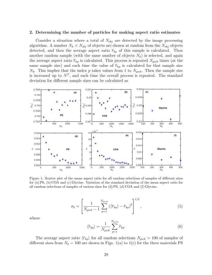
Consider a situation where a total of Nobj are detected by the image processingalgorithm. A number Nk < Nobj of objects are chosen at random from the Nobj objectsdetected, and then the average aspect ratio rkp of this sample is calculated. Thenanother random sample (with the same number of objects Nk) is selected, and againthe average aspect ratio rkp is calculated. This process is repeated Npick times (at thesame sample size) and each time the value of rkp is calculated for that sample sizeNk. This implies that the index p takes values from 1 to Npick. Then the sample sizeis increased up to NT , and each time the overall process is repeated. The standarddeviation for different sample sizes can be calculated as

Nk

0 500 1000 1500

〈rkp〉

0.7515

0.752

0.7525

0.753

0.7535

0.754

0.7545

Nk

0 500 1000 1500

σk

0.004

0.006

0.008

0.01

0.012

0.014

0.016

Nk

0 500 1000 1500 2000

〈rkp〉

0.187

0.188

0.189

0.19

0.191

Nk

0 500 1000 1500 2000

σk

×10-3

2

4

6

8

10

12

Nk

100 200 300 400 500

〈rkp〉

0.322

0.3225

0.323

0.3235

0.324

Nk

100 200 300 400 500

σk

0.006

0.008

0.01

0.012

0.014

0.016

(a)

COAPS

(b)

Glycine

(c)

(d)

PS COA

(e)

Glycine

(f)

Figure 1: Scatter plot of the mean aspect ratio for all random selections of samples of different sizesfor (a) PS, (b) COA and (c) Glycine. Variation of the standard deviation of the mean aspect ratio forall random selections of samples of various sizes for (d) PS, (d) COA and (f) Glycine.

σk =

1

Npick − 1

Npick∑p=1

(〈rkp〉 − rkp)21/2

, (5)

where

〈rkp〉 =1

Npick

Npick∑p=1

rkp. (6)

The average aspect ratio 〈rkp〉 for all random selections Npick = 100 of samples ofdifferent sizes from Nk = 100 are shown in Figs. 1(a) to 1(c) for the three materials PS

28

(Fig. 1(a)), CoA (Fig. 1(b)) and Glycine (Fig. 1(c)). The figures show small variationsof the mean aspect ratio with different sample size. However, the standard deviationσk consistently decreases with increasing sample size (as seen in Figs. 1(d) to 1(f)) asexpected. The results in Fig. 1 clearly show that the calculated mean value from theobjects detected in the images become more representative of the particles in the slurryas the number of detected objects increase. However, detecting more objects impliesprocessing more images and the time to do this depends on the acquisition frequencyof the image acquisition device and the image processing algorithm. Hence a decisionneeds to be made on the degree of accuracy that is sufficient for a particular process.Once that decision is made then the average aspect ratio can be retrieved at that samplesize. In any case, Fig. 1(d) to 1(f) show that the standard deviation σk begins to leveloff at sample size Nk ≈ 500. This implies that the error incurred in under sampling theparticles in the slurry become minimal for sample sizes Nk & 500.

3. Calculating volume based PSD

The technique for calculating the volume based PSD is the same as that presentedin [6]. A generalisation of the technique is necessary for the case of Method 2 (describedin subsection 6.2 of the main text) where multiple aspect ratios are assigned to particlesof the same characteristic length. The updated technique is described in this section.

Obtain the normalised number based PSD Xi as

Xi =Xi∑Ni=1Xi

, (7)

where Xi is the number based PSD calculated with the inversion algorithm. Thencalculate the CLD C∗j given as

C∗j =N∑i=1

AjiXi, (8)

where Aji is the transformation matrix corresponding to the number based PSD Xi.

The CLD C∗j could be associated with the number based PSD Xi (as in Eq. (8)) orthe volume based PSD Xv

i depending on the weighting applied to the matrix Aji. The

technique for weighting the matrix Aji in order to associate the transformed CLD C∗jto the volume based PSD is described below.

The volume based PSD is defined as [28]

Xvi =

XiV3i∑N

i=1 XiV 3i

, (9)

where Vi is the volume of the particle with characteristic size Li. The shape of theparticles in this work have been approximated with ellipsoids so that the volume ofeach particle is given as

Vi =4πaibici

3, (10)

29

where ai, bi and ci are the semi axes lengths in the x, y and z directions respectivelyof the ellipsoid of characteristic length Li = 2ai. In this case, the origin of coordinateshas been placed at the centre of the ellipsoid with the z direction parallel to the majoraxis of the ellipsoid. Assuming the axes lengths bi and ci are equal, then using bi = riai(where ri is the mean aspect ratio of all particles of the same characteristic length Li)in Eq. (10) and substituting in Eq. (9) gives

Xvi =

Xir2i a

3i∑N

i=1 Xir2i a

3i

. (11)

Substituting Eq. (11) in Eq. (8) gives

Cj =N∑i=1

AjiXv

i , (12)

where

Aji =Aji

r2iL3

i

Xv

i = Xvi

N∑i=1

Xir2iL

3

i . (13)

Equation (12) is the forward problem for the volume based PSD. If the weighted(due to Eq. (13)) volume based PSD X

v

i is known, then the CLD C∗j in Eq. (8) can becalculated using Eq. (12). In the case of Method 1 (described in subsection 6.1 of themain text) where the same aspect ratio is used for all the particles in the slurry, thenthe quantities Aji and X

v

i reduce to

Aji =Aji

L3

i

Xv

i = Xvi

N∑i=1

XiL3

i . (14)

Since the volume based PSD is usually not known, then an inverse problem can beformulated by searching for fitting parameters γvi which minimise an objective functionf of the form

f =M∑j=1

[C∗j −

N∑i=1

AjiXv

i

]2, (15)

whereXv

i = eγvi i = 1, 2, 3, . . . , N. (16)

This approach was demonstrated in [6] to correctly reproduce the volume based PSD.The function f is minimised using the Levenberg-Marquardth (the Matlab implemen-tation) using suitable initial trial solution for γvi . The initial trial solution for γvi is

30

constructed as γvi = ln(Xia3i ), where ai is the semi major axis length (defined in Eq.

(10)) for bin i and Xi is the number based PSD calculated from Eq. (17) of the maintext. When a smooth solution vector X

v

i is required, then Xi is calculated from Eq.(21) of the main text and the corresponding X

v

i is calculated from the same Eq. Moredetails on the procedure for choosing the smoothing parameter λ2 in Eq. (21) of themain text will be given in subsection 4.4.

4. Choice of algorithms parameters

The motivation for choosing different parameter values for the algorithms used inthis work are presented in the following subsections.

4.1. Choice of number of particle subgroups in each bin in Method 2

The Method 2 presented in subsection 6.2 of the main text outlines a techniquefor assigning multiple aspect ratios to particles of the same size. In this method, thecharacteristic particle size Li representing the size of particles in bin i is associatedwith multiple aspect ratios from rmini to rmaxi (see subsection 6.2 of the main text fordetails). To achieve this, the particles in bin i of characteristic size Li are subdividedinto Nr subgroups. Each subgroup is assigned an aspect ratio

rki ∈[rmini , rmaxi

]. (17)


CLD

(Counts)

0

0.01

0.02

0.03

0.04

0.05

0.06

Nr

5

10

15

20

rmin = 0.2

rmax = 0.7

L = 100

Figure 2: The mean CLD of a group of Nr particles of the same size L = 100µm but different aspectratios r ∈ [0.2, 0.7].

This then allows the construction of the 3D transformation matrix A from whichthe 2D transformation matrix A is constructed by averaging across slices of the 3Dmatrix as in Eq. 15 of the main text. Since the CLD for a particle of characteristicsize L reaches a peak at a size corresponding to the width of the particle [6], then eachcolumn of the average 2D matrix A (obtained using Eq. 15 of the main text) for aparticle of size L will contain oscillations. This is due to the variations in the widths

31

N10 20 30 40 50 60 70

‖C*−C‖

0

10

20

30

40

50

60


X

0

5

10

15

20

25

30 N10

30

50

70


CLD

(Counts)

0

20

40

60

80

100

120

140

(c)

(a)

(b)

Figure 3: (a) Variation of the L2 norm in Eq. (18) for different number of particle size bins N . (b) Thenumber based PSD for different number of particle size bins. (c) Corresponding CLDs for differentnumber of particle size bins.

of the particles of the same size but different aspect ratios. Hence, for more accuratecalculations, then the value of Nr needs to be chosen sufficiently large such that theoscillations are minimised.

Figure 2 shows the average CLD for a group of particle of the same characteristicsize L = 100µm. The Nr particles in each group are assigned uniformly spaced aspectratios from rmin = 0.2 to rmax = 0.7. The Fig. shows that the oscillations reduce asthe value of Nr increases. The oscillations become negligible at Nr & 20. However, avalue of Nr = 50 was used in the calculations in the main text for more accuracy.

4.2. Choice of number of particle size bins in Methods 1 and 2

It was demonstrated in [6] that the number of particle size bins N needed to getreasonable PSD estimate is of the order of N & 70. Since Method 1 (described insubsection 6.1 of the main text) uses a single representative aspect ratio to describethe shape of the particles (which is similar to the approach in [6]) in a slurry, then thenumber N = 70 of particle size bins was used in Method 1.

However, Method 2 (described in subsection 6.2 of the main text) assigns a range ofaspect ratios to particles of the same characteristic length L. This makes it necessary

32

to search for an optimum number of particle size bins which yields accurate solutionsand physically realistic PSDs.

Figure 2(a) shows the behaviour of the L2 norm defined in Eq. (19) of the maintext (repeated here for convenience)

‖C∗ −C‖ =√f1, (18)

where

f1 =M∑j=1

[C∗j −

N∑i=1

AjiXi

]2(19)

andXi = eγi , i = 1, 2, 3, . . . , N. (20)

The number based PSD Xi in Eq. (20) is the solution vector which minimises theobjective function f1 in (19), and the CLD Cj is calculated from the forward problemdescribed in Eq. (10) of the main text. The L2 norm in Eq. (18) measures the degreeof agreement between the experimentally measured CLD C∗j with the calculated CLDCj.

The L2 norm in Fig. 3(a) decreases as the number of particle size bins N increases,and begins to flatten out at about N = 50. This indicates that the calculations becomemore accurate as the number of particle size bins increases. However, the calculatednumber based PSD X in Fig. 3(b) becomes increasingly noisy as N increases. Theopposite situation holds for the calculated CLD C in Fig. 3(c) which becomes lessnoisy as N increases. Hence larger values of N give more accurate CLDs but thecorresponding PSDs become more physically unrealistic. This then leads to a choice ofN = 50 in the calculations shown in the main text. This is because the calculationsbecomes sufficiently accurate as suggested by Figs. 3(a) and 3(c). Furthermore, thecalculations are computationally more expensive at larger values of N .

4.3. Choice of λ1 value in Method 1

The Method 1 presented in subsection 6.1 of the main text uses a mean aspect ratioto represent the shape of the particles in a slurry. It involves the estimation of themean aspect ratio r from images, after which the best representative aspect ratio r issearched from the range

r ∈ [r −Nσr, r +Nσr], (21)

where σr is the standard deviation of all aspect ratios estimated from images and Nis the number of standard deviations chosen. Then for each aspect ratio r, a solutionvector X (which is the number based PSD) which minimises the objective function f1(given in Eq. (19)) is calculated.

When the value of N is made sufficiently large, then the calculated CLD Cj fromthe number based PSD Xi will match the experimentally measured CLD C∗j for one ormore values of r. The degree of agreement is quantified by calculating the L2 norm inEq. (18).

33

The desired situation would have been the case where the calculated CLD Cj atthe average aspect ratio r matches the experimentally measured CLD C∗j . However,this is usually not the case for a number of reasons. For example, the objects in theimages are not always in focus and a number of objects are rejected because they makecontact with the image frame. Also the particles do not all have the same shape, sothat the estimated average aspect ratio r will not necessarily be representative of allthe particles in the slurry. Hence it is necessary to search for a representative aspectratio from a suitable range around r as given in Eq. (21). The search for a suitableaspect ratio is similar to the situation presented in [6], however in this work, the searchrange has been narrowed down by means of the estimated average aspect ratio r fromthe images.

r

0.1 0.2 0.3 0.4 0.5 0.6

√

f 1

5

10

15

20

25

r*

r

0.1 0.2 0.3 0.4 0.5 0.6 0.7

√

f 1

10

20

30

40

50

60

70

r*

r

0.1 0.2 0.3 0.4 0.5 0.6

∑iX

2 i

0

100

200

300

400

500

r

0.1 0.2 0.3 0.4 0.5 0.6 0.7

∑iX

2 i

0

500

1000

1500

2000

r

0.4 0.5 0.6 0.7 0.8 0.9 1

√

f 1

30

40

50

60

70

80

90

r*

r

0.4 0.5 0.6 0.7 0.8 0.9 1

∑iX

2 i

50

55

60

65

70

(b) (c)

(e) (f)

PS

COAGlycine

Glycine

(a)

(d)

COA

PS

Figure 4: The L2 norm in Eq. (18) for (a) PS, (b) COA and (c) Glycine. The square of the size ofthe number based PSD retrieved from the objective function f1 in Eq. (18) for (d) PS, (e) COA and(f) Glycine.

Since the inversion is not necessarily carried out at the estimated average aspectratio r, then a situation similar to that discussed in [6] arises, whereby the L2 normin Eq. (18) becomes nearly flat after some critical aspect ratio r∗. This can be seenfor PS (r∗ ≈ 0.6), COA (r∗ ≈ 0.3) and Glycine (r∗ ≈ 0.4) in Figs. 4(a) to 4(c). Thecritical aspect ratio shifts to the left as the aspect ratio of the particles decreases as canbe seen by comparing Figs 4(a) to 4(c) to Figs. 2(a) to 2(c) in the main text.

This calls for a technique to retrieve a unique aspect ratio which is reasonable whencompared with the shape of the particles of interest. An objective function f2 whichimposes a penalty on the size of the calculated number based PSD Xi was introduced

34

λ1

10-2 10-1 100 101 102 103 104 105

T1,T

2

100

102

104

106

λ*1

T1

T2

r = 0.6

λ1

10-2 10-1 100 101 102 103 104 105

T1,T

2

100

102

104

106

λ*1

T1

T2

r = 0.7

λ1

10-2 10-1 100 101 102 103 104 105

T1,T

2

100

102

104

106

λ*1

T1

T2

r = 0.8

λ1

10-2 10-1 100 101 102 103 104 105

T1,T

2

100

102

104

106

λ*1

T1

T2

r = 0.9

(a) (b)

(d)(c)

PS

Figure 5: The behaviour of the terms T1 and T2 in Eq. (22) for PS at the aspect ratios indicated in(a) to (d).

in [6] to pick this unique aspect ratio. The objective function f2 is given as (same asEq. (20) in the main text)

f2 =M∑j=1

[C∗j −

N∑i=1

AjiXi

]2︸︷︷︸

T1

+λ1

N∑i=1

X2i︸︷︷︸

T2

. (22)

The term T1 is the original objective function f1 in Eq. (19), and the parameter λ1sets the level of penalty on the PSD size which is contained in the term T2. The formof the penalty term was chosen (as discussed in [6]) because the total variation of thesolution vector shows a general increase with aspect ratio as seen in Figs. 4(d) to 4(f)for PS, COA and Glycine. If the value of λ1 is chosen carefully, then a unique aspectratio can be found which is reasonable when compared with the shape of the particles.The method for estimating λ1 is outlined below.

The idea is to estimate a value of λ1 such that the penalty term T2 just balances

35

r0.4 0.5 0.6 0.7 0.8 0.9 1

λ* 1

30

50

102

150

250

r0.4 0.5 0.6 0.7 0.8 0.9 1

T1+T

2

1000

3000

5000

7000

r = 1

λ1 ≈ 0.95


X(µm)−

1

0

0.02

0.04

0.06

0.08

0.1

0.12

r = 1

λ1 ≈ 0.95


CLD

(Counts)

0

50

100

150

200

250λ1 = 0

λ1 ≈ 0.95

(a) (b)

(c) (d)

PS

Figure 6: The behaviour (with aspect ratio) of the critical value of λ1 at which the T2 term first crossesthe T1 term in Eq. (22) for PS. (b) The objective function f2 in Eq. (22) with aspect ratios for PS.(c) The number based PSD (for PS) calculated at r = 1 where the objective function in (b) reaches aminimum. (d) The corresponding CLD (black line) to the number based PSD in (c). The red line isthe calculated CLD at λ1 = 0 and the symbols are the experimentally measured CLD.

the term T1 in Eq. (22). The procedure is as follows:For a given aspect ratio r, obtain an initial estimate λ01 from

λ01 =T 01

T 02

, (23)

where T 01 and T 0

2 are computed from Eq. (10) as

T 01 =

M∑j=1

[C∗j −

N∑i=1

AjiXi

]2

T 02 =

N∑i=1

X2i . (24)

36

r0.1 0.2 0.3 0.4 0.5 0.6

λ* 1

10-1

100

101

102

r0.1 0.2 0.3 0.4 0.5 0.6

T1+T

2

0

100

200

300

400

500

600

700

r = 0.3

λ1 ≈ 0.45

Particle length. (µm)101 102 103

X(µm)−

1

0

0.02

0.04

0.06

0.08

0.1

r = 0.3

λ1 ≈ 0.45


CLD

(Counts)

0

10

20

30

40

50

60

λ1 = 0

λ1 ≈ 0.45

(a) (b)

(d)(c)

COA

Figure 7: Same as in Fig. 6 but for COA.

Then construct the objective function f2 in Eq. (22) for different values of λ1 from therange

λ1 ∈ . . . , λ01(∆λ1)−2, λ01(∆λ1)−1, λ01, λ01∆λ1, λ01(∆λ1)2, . . . , (25)

where the value of ∆λ1 chosen depends on the data set being analysed. The value of∆λ1 = 5 was used for the PS, COA and Glycine samples in this work. Then the valueof λ1 at which the term T2 (in Eq. (22)) just becomes equal to the term T1 (also in Eq.(22)) is chosen as the optimum value of λ1 for that aspect ratio. The behaviour of theterms T1 and T2 for different aspect ratios for PS are shown in Figs. 5(a) to 5(d). Thesituation is the same for COA and Glycine. The term T2 just matches the term T1 ata critical value of λ1 (indicated as λ∗1) in Figs. 5(a) to 5(d). However, as Figs. 5(a) to5(d) show, there is a wide disparity in the values of λ∗1 as the aspect ratio increases.This is seen more clearly in Fig. 6(a) which shows the variation of λ∗1 with aspect ratior for PS, and in Fig. 7(a) and 8(a) for COA and Glycine respectively. This suggeststhat the large variance in the values of λ∗1 be removed before a meaningful average canbe made. This is achieved by normalising the values of λ∗1 by the standard deviation ofthe λ∗1 values for a particular sample and then taking the mean value as given in Eq.

37

r0.1 0.2 0.3 0.4 0.5 0.6 0.7

λ* 1

10-2

10-1

100

101

102

r0.1 0.2 0.3 0.4 0.5 0.6 0.7

T1+T

2

0

1000

2000

3000

4000

5000

λ1 ≈ 0.41

r = 0.4

Particle length. (µm)101 102 103

X(µm)−

1

0

0.02

0.04

0.06

0.08

0.1

0.12

0.14

0.16

λ1 ≈ 0.41

r = 0.4


CLD

(Counts)

0

20

40

60

80

100

120 λ1 = 0

λ1 ≈ 0.41

(c) (d)

(a) (b)

Glycine

Figure 8: Same as in Fig. 6 but for Glycine.

(26)

λ1 =1

σλNr

Nr∑q=1

λ∗1(rq), (26)

where Nr is the number of aspect ratios at which the calculations were performed andσλ is the standard deviation of the λ∗1 values. Normalising the data set (the values ofλ∗1) by their standard deviation reduces the large variance in the set so that the varianceof the data set becomes unity. The estimated λ1 (by Eq. (26)) is just large enough toproduce a shallow minimum in the objective function f2. Then the predicted aspectratio is consistent with the actual shape of the particles.

The estimated value of λ1 ≈ 0.95 from Eq. (26) for PS gives an estimated aspectratio of r = 1 as seen in Fig. 6(b). This is a reasonable estimate of aspect ratio since theparticles of PS are near spherical as seen in Fig. 2(a) of the main text. The estimatednumber based PSD at λ1 ≈ 0.95 and r = 1 (using the objective function f2 in Eq. (22))is shown in Fig. 6(c). The corresponding calculated CLD at λ1 ≈ 0.95 and r = 1 isshown by the black solid line in Fig. 6(d). The experimentally measured CLD for PSis shown by the symbols in Fig. 6(d). The calculated CLD at λ1 = 0 (using f1 in Eq.(19)) and r = 1 for PS is shown by the red solid line in Fig. 6(d).

38

λ2

10-5 10-3 10-1 101 103 105 107

T3,T

4

100

102 T3

T4


CLD

(Counts)

0

50

100

150

200

250

Expt


X(µm)−

1

0

0.02

0.04

0.06

0.08

0.1

0.12λ2 = 0

λ2 = 10−3

λ2 = 10−2

λ2 = 10

λ2

10-23 10-21 10-19 10-17 10-15 10-13 10-11

T3,T

4

10-20

10-10

100

T3

T4


Xv(µm)−

1

×10-3

0

2

4

6

8 λ2 = 0


C*

0

1

2

3

4

5

6

C*

(a)

(b) (c)

PS

(d)

(e) (f)

Figure 9: (a) The terms T3 and T4 (for the number based PSD) in Eq. (27) at various values of λ2for PS. (b) The number based PSD (for PS) computed from Eq. (27) at the various values of λ2indicated. (c) The calculated CLDs corresponding to the number based PSDs in (b). The black line isthe experimentally measured CLD. (d) The terms T3 and T4 (for the volume based PSD) at differentvalues of λ2 in Eq. (27). (e) The calculated (from Eq. (27)) volume based PSD for PS at the value ofλ2 indicated. All calculations performed by Method 1 described in subsection 6.1 in the main text.

The number based PSD for PS in Fig. 6(c) shows large particle counts at smallparticle sizes close to 10µm. This is because of surface roughness in the PS particleswhich contribute a significant number of short chords approximately less than 10µm tothe CLD. The counts from these short chords are not very obvious in Fig. 6(d) due tothe concentration of the PS sample which makes the longer chords dominate the CLD.However, the counts from short chords are more obvious in a more dilute system.

Both the red and black solid lines in Fig. 6(d) have a near perfect match with theexperimentally measured CLD (symbols in Fig. 6(d)), which shows that the estimatedvalue of λ1 by Eq. (26) is reasonable.

Figure 8(a) shows that the behaviour of λ∗1 as a function of aspect ratio, for COAis similar to the case of PS. The estimated value of λ1 ≈ 0.45 (using Eq. (26)) gives anaspect ratio of r = 0.3 (using f2 in Eq. (22)) as seen in Fig. 7(b). This estimated aspectratio agrees with the needle-like shape of the particles of COA as seen in Fig. 2(b) ofthe main text. The estimated number based PSD at λ1 ≈ 0.45 and r = 0.3 for COAis shown in Fig. 7(c). The corresponding calculated CLD at λ1 ≈ 0.45 and r = 0.3 forCOA (shown by the black solid line in Fig. 7(d)) shows a very good agreement with themeasured CLD (symbols in Fig. 7(d)). The calculated CLD at λ1 = 0 and r = 0.3 isvery close to the calculated CLD at λ1 ≈ 0.45 similar to the case of PS. This indicates

39

λ2

10-5 10-3 100 102 105

T3,T

4

10-2

100

102

T3

T4


X(µm)−

1

0

0.02

0.04

0.06

0.08

0.1λ2 = 0

λ2 = 0.05

λ2 = 1

λ2 = 10


CLD

(Counts)

0

10

20

30

40

50

60Expt

λ2

10-14 10-11 10-8 10-5

T3,T

4

10-6

10-4

10-2

100

T3

T4


Xv(µm)−

1

×10-3

0

2

4

6

8λ2 = 0

λ2 = 10−10

λ2 = 10−7

λ2 = 10−3


C*

0

0.2

0.4

0.6

0.8

C*

(a) (b) (c)

COA

(f)(e)

(d)

Figure 10: Same as in Fig. 9 but for COA.

that the estimated value of λ1 is just at the right level.The situation for Glycine is similar to those of the PS and COA samples. The λ∗1

values also show a decrease with aspect ratio as seen in Fig. 8(a). The application ofEq. (26) leads to an estimated λ1 ≈ 0.41 and subsequently r = 0.4. The estimatedvalue of r = 0.4 also agrees with the prism-like shape of the particles of Glycine. Similarto the cases of PS and COA, the estimated value of λ1 ≈ 0.41 is just at the right level.This is because the calculated CLD at λ1 ≈ 0.41 and r = 0.4 (black solid line in Fig.8(d)) has a near perfect match with the calculated CLD at λ1 = 0 and r = 0.4 (redsolid line in Fig. 8(d)) and both show a near perfect match with the measured CLD(symbols in Fig. 8(d)).

4.4. Choice of λ2 value for both Methods 1 and 2

The number based PSDs estimated from Eq. (22) are not necessarily smooth asin the cases of the PS, COA and Glycine samples seen in Figs. 6(c), 7(c) and 8(c)respectively. They contain different degrees of oscillations. This is because the penaltyfunction T2 in Eq. (22) is not guaranteed to force the algorithm to search for a smoothsolution. Similarly, when the volume based PSDs are estimated from Eq. (15), theymay not necessarily be smooth.

In order to retrieve smooth solutions a new objective function was introduced insection 7 of the main text. This objective function f3 (which contains a penalty functionthat enforces smoothness) is defined in Eq. (15) of the main text but repeated here for

40

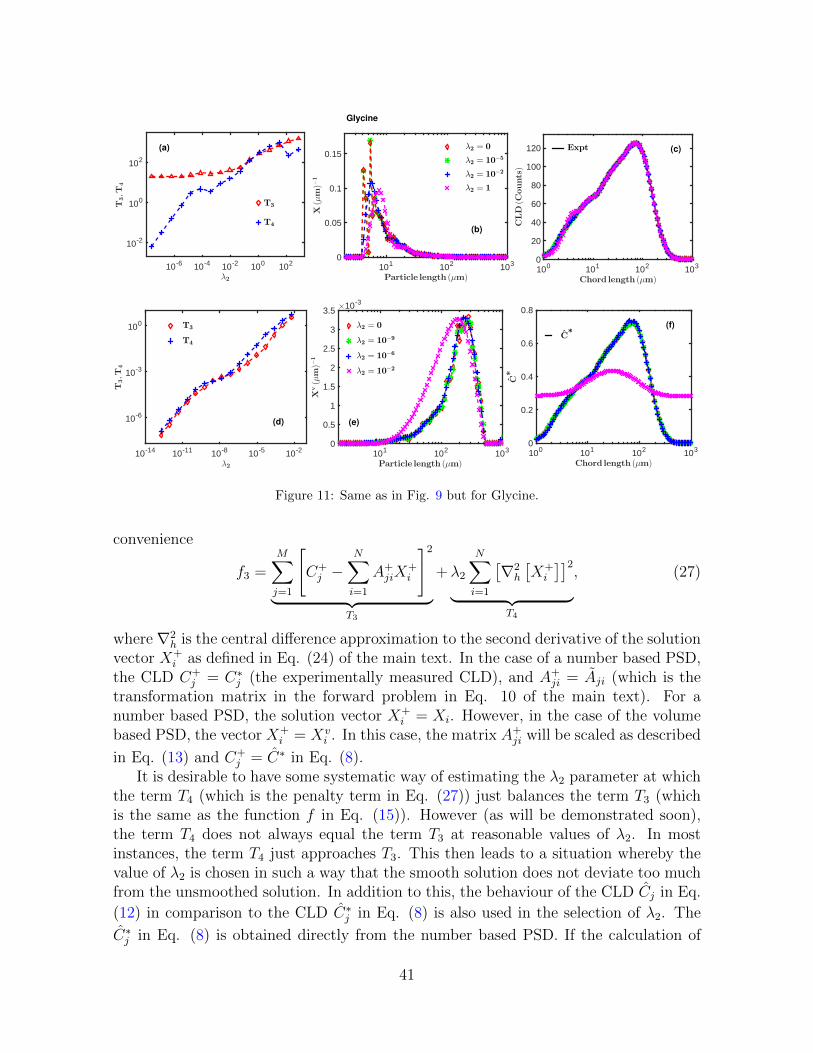
λ2

10-6 10-4 10-2 100 102

T3,T

4

10-2

100

102

T3

T4


X(µm)−

1

0

0.05

0.1

0.15λ2 = 0

λ2 = 10−5

λ2 = 10−2

λ2 = 1


CLD

(Counts)

0

20

40

60

80

100

120 Expt

λ2

10-14 10-11 10-8 10-5 10-2

T3,T

4

10-6

10-3

100 T3

T4


Xv(µm)−

1×10-3

0

0.5

1

1.5

2

2.5

3

3.5

λ2 = 0

λ2 = 10−9

λ2 = 10−6

λ2 = 10−2


C*

0

0.2

0.4

0.6

0.8

C*

(a)

(b)

(c)

(d)

Glycine

(f)

(e)


convenience

f3 =M∑j=1

[C+j −

N∑i=1

A+jiX

+i

]2︸︷︷︸

T3

+λ2

N∑i=1

[∇2h

[X+i

]]2︸︷︷︸

T4

, (27)

where∇2h is the central difference approximation to the second derivative of the solution

vector X+i as defined in Eq. (24) of the main text. In the case of a number based PSD,

the CLD C+j = C∗j (the experimentally measured CLD), and A+

ji = Aji (which is thetransformation matrix in the forward problem in Eq. 10 of the main text). For anumber based PSD, the solution vector X+

i = Xi. However, in the case of the volumebased PSD, the vector X+

i = Xvi . In this case, the matrix A+

ji will be scaled as described

in Eq. (13) and C+j = C∗ in Eq. (8).

It is desirable to have some systematic way of estimating the λ2 parameter at whichthe term T4 (which is the penalty term in Eq. (27)) just balances the term T3 (whichis the same as the function f in Eq. (15)). However (as will be demonstrated soon),the term T4 does not always equal the term T3 at reasonable values of λ2. In mostinstances, the term T4 just approaches T3. This then leads to a situation whereby thevalue of λ2 is chosen in such a way that the smooth solution does not deviate too muchfrom the unsmoothed solution. In addition to this, the behaviour of the CLD Cj in Eq.

(12) in comparison to the CLD C∗j in Eq. (8) is also used in the selection of λ2. The

C∗j in Eq. (8) is obtained directly from the number based PSD. If the calculation of

41


X(µm)−

1

0

0.05

0.1

0.15 λ2 = 0.1

λ2 = 10

λ2 = 1

λ2 = 0


CLD

(Counts)

0

10

20

30

40

50

60

Expt

λ2

10-10 10-6 10-2 102 105 108 1011

T3,T

4

10-5

100

105

T3

T4

λ2

10-20 10-15 10-10 10-5 100 105

T3,T

4

10-15

10-10

10-5

100

T3

T4


Xv(µm)−

1×10-3

0

2

4

6

8 λ2 = 0

λ2 = 10−8

λ2 = 3× 10−6

λ2 = 10−2


C*

0

0.1

0.2

0.3

0.4

0.5

0.6

C*

(b)

(c)(a)

(d) (e) (f)

COA

Figure 12: Similar to Fig. 9 but calculations by Method 2 (described in subsection 6.2 of the maintext) for COA.

the volume based PSD from Eq. (27) is correct, then the CLD Cj obtained from this

volume based PSD using Eq. (12) should match the CLD C∗j from Eq. (8). Hence a

value of λ2 is accepted if the CLD Cj calculated from the volume based PSD (obtained

at that value of λ2) does not deviate significantly from the CLD C∗j , and the volumebased PSD (calculated at the specified value of λ2) does not deviate significantly fromthe volume based PSD calculated at λ2 = 0. Similarly, the calculated number basedPSD from Eq. (27) is rejected it its corresponding CLD (calculated from the forwardproblem in Eq. (10) of the main text) deviates significantly from the measured CLD.

Figure 9(a) shows the behaviour of the terms T3 and T4 for different values of λ2for PS (for the case of the number based PSD) at aspect ratio1 r = 1. The term T4approaches the term T4 for λ2 & 105. The number based PSD obtained at λ2 = 10−3

(shown by the green asterisks in Fig. 9(b)) has about the same degree of oscillations asthe number based PSD obtained at λ2 = 0 (red diamonds in Fig. 9(b)). At λ2 = 10−2

the number based PSD (blue crosses in Fig. 9(b)) becomes smoother and has a peakwhich is close to the unsmoothed PSD obtained at λ2 = 0. However, as the value of λ2is increased further, the number based PSD drifts significantly from the unsmoothedPSD as seen by the position of the peak of the number based PSD obtained at λ2 = 10

1This is the case where the particles are assigned a single representative aspect ratio estimatedusing f2 in Eq. (22). This approach was referred to as Method 1 in subsection 6.1 of the main text.

42

λ2

10-12 10-8 10-4 100 104 108

T3,T

4

10-5

100

105

T3

T4


X(µm)−

1

0

0.05

0.1

0.15

0.2λ2 = 0

λ2 = 10−4

λ2 = 10−2

λ2 = 1


CLD

(Counts)

0

20

40

60

80

100

120

Expt

λ2

10-30 10-25 10-20 10-15 10-10 10-5

T3,T

4

10-30

10-20

10-10

100

T3

T4


Xv(µm)−

1

×10-3

0

1

2

3

4

λ2 = 0

λ2 = 10−8

λ2 = 10−5

λ2 = 10−2


C*

0

0.1

0.2

0.3

0.4

0.5

0.6

C*

(a) (c)

(b)

Glycine

(e) (f)(d)


(shown by the magenta crosses in Fig. 9(b)).Even though the calculated CLD at λ2 = 10 (in Fig. 9(c)) still matches the experi-

mentally measured CLD, the significant drift of the peak of the number based PSD atλ2 = 10 (seen in Fig. 9(b)) suggests that a smaller value of λ2 is appropriate to obtaina smooth number based PSD for this PS sample. Hence the value of λ2 = 10−2 waschosen for this sample.

In the case of the volume based PSD (for PS), the term T4 (in Fig. 9(d)) approachesthe term T3 at sufficiently large values of λ2 similar to the case of the number based PSDin Fig. 9(a). The unsmoothed (λ2 = 0) volume based PSD estimated for PS is shownin Fig. 9(e). Since the volume based PSD at λ2 = 0 does not contain oscillations (asseen in Fig. 9(e)), then the computed solution at λ2 = 0 was accepted. Furthermore,the CLD Cj (for PS) calculated at λ2 = 0 (red diamonds in Fig. 9(f)) matches the

CLD C∗j (solid black line in Fig. 9(f)).The case of COA is similar to that of PS. The term T3 never crosses the term T4

within reasonable values of λ2 as seen in Fig. 10(a). The λ2 values are said to be unrea-sonable when the smoothed number based PSD begins to drift from the unsmoothedsolution (obtained at λ2 = 0) as seen in Fig. 10(b). This is also reflected in the cal-culated CLDs which begin to deviate significantly from the experimentally measuredCLD when the λ2 values become too large as in Fig. 10(c).

The oscillations at the peak of the unsmoothed (λ2 = 0) number based PSD hadbeen smoothed out in the number based PSD obtained at λ2 = 0.05 as in Fig. 10(b).The corresponding CLD at λ2 = 0.05 has a near perfect match with the experimentallymeasured CLD for COA as in Fig. 10(c). Since the peaks of the PSDs obtained at the

43

Figure 14: The shape descriptor (defined in Eq. (4) of the main text) for individual particles of(a) PS, (b) COA and (c) Glycine. The mean shape descriptor with error bars for (d) PS, (e) COA and(f) Glycine. Each error bar is one standard deviation (standard deviation of the distances from thecentroid for all objects detected at each angular position) above and below each data point.

higher values of λ2 (λ2 & 0.05) drift from the unsmoothed number based PSD (Fig.10(b)) and their corresponding CLDs deviate from the experimentally measured CLD,then the CLD corresponding to the number based PSD obtained at λ2 = 0.05 waspresented in Fig. 9(b) of the main text.

Similar to the T4 term for the number based PSD, the T4 term for the volume basedPSD does not cross the T3 term at reasonable values of λ2 (see Fig. 10(d)). The valueof λ2 = 10−7 was chosen for smoothing the volume based PSD for COA. This is becauseFig. 10(e) shows that the peaks of the calculated volume based PSDs drift significantlyfrom the unsmoothed (λ2 = 0) volume based PSD for large values of λ2 (λ2 & 10−7).Similarly, the CLD Cj deviates significantly from the CLD C∗j for λ2 & 10−7 as seen inFig. 10(f).

Unlike the cases of the PS and COA samples, the T4 term for the number basedPSD crosses the T3 term (at λ2 ≈ 0.4) for Glycine as seen2 in Fig. 11(a). However, asFig. 11(b) shows, the oscillations in the unsmoothed solution (at λ2 = 0) are alreadysmoothed out for a smaller value of λ2 = 0.01 < 0.4. Similarly to the cases of the PSand COA samples, the peak of the smoothed number based PSD drifts from the peak

2This is one of the few instances where the T4 term crosses the T3 term in Eq. (27).

44

Figure 15: Illustration of the scheme to combine the windowing technique introduced in [6] with aspectratio from images.

of the unsmoothed PSD for large values of λ2 (as in the case of λ2 = 1 in Fig. 11(b)).Similarly, the calculated CLD deviates from the experimentally measured CLD at largevalues of λ2 as seen in the case of λ2 = 1 in Fig. 11(c). Hence the value of λ2 = 0.01was chosen for the number based PSD for Glycine.

Also in contrast to the cases of PS and COA, the T4 term of the volume based PSDis about equal to the T3 term (for λ2 . 10−6) of the in the case of Glycine as seenin Fig. 11(d). However, the selection of λ2 for the volume based PSD is done in amanner similar to those of PS and COA. The value of λ2 = 10−6 was chosen for thevolume based PSD for Glycine since the left shoulder seen in the volume based PSDat λ2 = 0 (Fig. 11(e)) becomes less obvious for λ2 & 10−6. Also, the CLD Cj deviates

significantly from the CLD C∗j for λ2 & 10−6 as seen in Fig. 11(f).In the case3 of Method 2, the behaviour of the terms T3 and T4 in Eq. (27) is similar

to the case of Method 1. Figure 12(a) shows the behaviour of the terms T3 and T4 (inEq. (27)) with λ2 for COA. The term T4 does not cross the term T3 (within reasonablevalues of λ2). The term T4 becomes nearly equal to the term T3 for λ2 & 0.1. Thenumber based PSD estimated for COA at λ2 = 0.1 is shown in Fig. 12(b). It has aboutthe same degree of fluctuation (at the peak) as the estimated number based PSD atλ2 = 0 (in Fig. 12(b)). However, as λ2 is increased to 1, the fluctuations at the peak

3The case where multiple aspect ratios are assigned to different particles of the same length asdescribed in subsection 6.2 of the main text

45

are penalised as seen in Fig. 12(b). As the value of λ2 is increased further to λ2 = 10,the peak of the number based PSD begins to drift from the unsmoothed number basedPSD as seen in Fig. 12(b). At this value of λ1 = 10, the calculated CLD begins todeviate from the experimentally measured CLD and calculated CLDs at smaller valuesof λ2. This situation is shown in Fig. 12(c).

The behaviour of the T3 and T4 terms for the volume based PSD (for COA) issimilar to the case of the number based PSD. The T4 term shows a near linear increasefor λ2 . 10−8 as seen in Fig. 12(d). This suggests that the smoothing effect of the T4term is ineffective at these small values of λ2. However, the smoothing effect kicks infor λ2 & 10−8. At this value of λ2 = 10−8, the fluctuations in the estimated volumebased PSD only reduce slightly as seen in Fig. 12(e). However, at λ2 ≈ 3 × 10−6,the fluctuations smoothen out as seen in Fig. 12(e). As the value of λ2 is increased to10−2, the peak of the estimated volume based PSD begins to drift from the unsmoothedvolume based PSD as seen in Fig. 12(e). Also, the minor peak of the estimated volumebased PSD at λ2 = 10−2 decreases significantly. Furthermore, the calculated CLD Cj at

λ2 = 10−2 deviates significantly from the CLD C∗j as seen in Fig. 12(f). This indicatesthat the value of λ2 = 3× 10−6 is more suitable for the COA sample.

The situation for Glycine is similar to that of COA where the T4 term does not crossthe T3 term as seen in Fig. 13(a). Similarly, Fig. 13(b) suggests a suitable value of λ2for the number based PSD to be λ2 ≈ 10−2. Figure 13(c) also show that the calculatedCLD for the higher value of λ2 = 1 deviates slightly from the experimentally measuredCLD and the calculated CLDs at smaller values of λ2. The situation for the volumebased PSD is similar to that of COA. The smoothing effect of the T4 term kicks in atλ2 & 10−12 (Fig. 13(d)), and Fig. 13(e) suggests a suitable value of λ2 to be about10−5. This is also supported by Fig. 13(f) which shows that the CLD Cj deviates

significantly from the CLD C∗j for λ2 > 10−5.

4.5. Image processing algorithm parameters

The tunable parameters of the image processing algorithm described in section 4of the main text are summarised in Table 1. The parameter names in Table 1 are thesame as they were used in the code. The description of each parameter and its effect isgiven in Table 1.

4.6. Shape descriptors for individual objects

The mean aspect ratio r (used in Method 1 to construct a range of aspect ratioswithin which to search for a representative value) is obtained from the mean shapedescriptor of the objects from images as outlined in section 4 of the main text. Althoughthis mean shape descriptor is reasonably smooth as seen in Figs. 5(d), 5(e) and 5(f)of the main text, the shape descriptors for individual objects contain some degree ofoscillations. Figures 14(a), 14(b) and 14(c) show the shape descriptors for the individualparticles in the PS, COA and Glycine samples respectively. They contain differentdegrees of oscillations due to variations in the shapes of the particles. There is also acontribution from errors in the detection of particles’ boundaries because some particles

46

Table 1: Summary of tunable parameters of the image processing algorithm.

Parameter name Description Defaultvalue

Effect

Step 1: Traditional spatial median filtering is used to reduce noise in theimage.prefilter.median size Size of the fil-

ter window5 pixels The bigger the value the stronger the

effect. Effect is similar to a low pass fil-ter but preserves sharp (high contrast)edges in the image.

Step 2: A classical method of high pass filter (Laplacian of Gaussian andthreshold) is used to detect objects edges.object detector.Logsize

Size of the fil-ter window

89 pixels Large window sizes remove noise at theexpense of blurred objects.

object detector.Logpower

Gaussiancurve stan-dard devia-tion

0.23327 The bigger the value, the lower the con-trast needs to be at the edges for theedge be detected; this does increase therisk of misclassifying noise as edge.

object detector.edgethreshold

Threshold ofdetection

251 The higher the value, the sharper theedge has to be in order to be classifiedas edge. This reduces noise at the ex-pense of not detecting an edge if thevalue is too high.

Step 3: Object processing - detected objects are filtered to discard objectsthat do not possess desirable properties.objectprocessing.imclosesize

Size of diskfor the op-eration ofmorphologi-cal closing

8 pixels The bigger the value, the bigger thegaps in the object that will be filled.This reduces noise in the result. Thetrade-off is that the shape of the origi-nal object might be lost.

objectprocessing.filterarea minimum

Objects arealess thanspecifiedvalue arediscarded

900 pixels If an object is too small, the chance isthat it is noise. The bigger the value,then the more that small objects arediscarded. The trade-off is that poten-tially useful objects can be discarded.

In the final stage, solid objects are reduced to their boundary only, andthe coordinates of pixels on the boundaries are reported.borderprocessing.borderthickness

Desired thick-ness of theborder

1 pixel Optionally, setting this to 2 pixels willproduce higher angular resolution out-put. However, this is often not needed.

47

are only partly in focus. There is also a contribution from impurities in the samples.This leads to the large error bars on the mean shape descriptors for the three samples asseen in Figs. 14(d), 14(e) and 14(f). The length of each error bar in Figs. 14(d), 14(e)and 14(f) is two times the standard deviation of the distance from the centroid. Thesize of the error bars in Figs. 14(d), 14(e) and 14(f) strongly indicates that a reliableestimate of the PSD cannot be made from current in-line imaging sensors (the PVMin this case) alone. Hence the need to combine the imaging data with CLD data ascarried out in this work. However, the use of image data along with CLD data leadsto significant improvements in the PSD estimates. The contribution to the size of theerror bars by the variation in particle shape justifies the method which assigns multipleaspect ratios to particles of the same length rather than using an average aspect ratiofor all particles in the slurry.

5. Integrating windowing technique with aspect ratios from images in Method2

The windowing technique developed in [6] allows the values of Lmin and Lmax tobe estimated in-line using the bin boundaries of the CLD histogram. The quantitiesLmin and Lmax (defined in Eqs. (8) and (9) of the main text) are the minimum andmaximum sizes of the particles in a slurry. The size of a window is the number of CLDbins covered by that window, and the position of a window is set by the index P . Forexample, in the case shown in Fig. 15, a window of size 2 is placed at different positions(indicated by P = 1, 2, . . . , 7 in the Fig.) along the CLD bin boundaries. At the firstwindow position (indicated by P = 1 in Fig. 15), the values of s1 and s3 (where s1and s3 are the chord lengths corresponding to the boundaries covered by the windowat P = 1) are assigned to Lmin and Lmax respectively. Similarly, at P = 2, Lmin = s2and Lmax = s4 and so on [6].

Consider a simple distribution of aspect ratios shown by the blue circles in Fig. 15.The aspect ratios in Fig. 15 were simulated using uniformly distributed random num-bers in the interval (0,1). In a real experiment, the aspect ratios will be estimated fromimages. The aspect ratios r ∈ [rmin, rmax] correspond to particle sizes L ∈ [Limmin, L

immax]

as indicated in Fig. 15, where Limmin and Limmax are the minimum and maximum particlesizes obtained from all the images analysed.

The chord lengths corresponding to the bin boundaries of the CLD histogram coverthe range s1 = 1µm to sM+1 = 103µm as indicated in Fig. 15, where M is the numberof CLD bins. However, the particle sizes estimated from images do not cover thisrange (Limmin > 1µm and Limmax < 103µm as illustrated in Fig. 15). This calls forappropriate approximations in the situations where the Lmin and Lmax values returnedby the window do not lie entirely within the range set by Limmin and Limmax. The followingprocedure was implemented in this work:

1. At position P = 1 where Lmax < Limmin, assign rmax to all Nr particle subgroups(the particle subgroups were discussed in subsection 6.2 of the main text). This

48

approach was adopted because Figs. 6(b) and 6(c) of the main text suggest thatthe small particles are more rounded than the larger particles.

2. At P = 2 where Lmin < Limmin and Limmin < Lmax < Limmax, assign rmax to the first50% of the Nr subgroups and for the remaining 50%, assign aspect ratios (fromimages) corresponding to particle sizes between Limmin and Lmax.

3. At P = 4 where Limmin < Lmin < Limmax and Limmin < Lmax < Limmax, assign aspectratios (from images) corresponding to particle sizes between Lmin and Lmax to allNr subgroups.

4. At P = 6 where Limmin < Lmin < Limmax and Lmax > Limmax, assign aspect ratios(from images) corresponding to particle sizes between Lmin and Limmax to the first50% of the Nr subgroups, and assign aspect ratio r to the remaining 50% ofthe Nr subgroups, where r is the mean aspect ratio estimated from images. Thisapproach was adopted because Figs. 6(b) and 6(c) suggest that the larger particleshave aspect ratio closer to the mean value than to rmax.

5. At P = 7, where Lmin > Limmax, assign aspect ratio r to all Nr subgroups.

This approach allows the computation of the 3 D matrix defined in Eq. (15) of themain text.

6. Comparison of estimated PSD from images and PSDs from Methods 1and 2

Even though the objects detected from the images suffer from focusing problems asdiscussed in the main text, an estimate of the PSD from the images can be made. Forthis purpose the particles are treated as ellipsoids whose two minor axes lengths areequal (as described in section 3) and their semi major axes lengths are given as a. Thenumber based PSD for each sample (COA and Glycine) is obtained from a histogramof the counts of particle lengths L = 2a using a geometrically spaced grid (with N = 70bins) running from particle lengths of 1µm to 1000µm. The number based PSD is thennormalised as described in Eq. (26) of the main text.

The number based PSDs X estimated in this way for COA and Glycine are shownin Fig. 16(a). The PSDs are a bit noisy due to the focusing issues in the images. Theleft tails of the PSDs terminate close to 30µm since objects smaller than about thissize are discarded from the image analysis as explained in subsection 4.1 of the maintext. Hence small particles of lengths . 30µm are not counted in this estimate of thenumber based PSD. As the small particles are not counted, then the peak of the numberbased PSD (for COA) in Fig. 16(a) is shifted to the right of the number based PSDsestimated for COA in Fig. 10(b) (by Method 1) and Fig. 12(b) (by Method 2). Asimilar situation holds for the number based PSD estimated for Glycine in Fig. 11(b)(by Method 1) and in Fig. 13(b) by Method 2.

49


X(µm)−

1

0

0.002

0.004

0.006

0.008

0.01

Glycine

COA


Xv(µm)−

1

×10-3

0

2

4

6

8Method1

Method2


Xv(µm)−

1

×10-3

0

1

2

3

Method2

Method1

(a)

(b)

COA Glycine

(c)

Figure 16: (a) Estimated (from imaging data) number based PSD for the COA and Glycine samples(as indicated in the Fig.). This estimate does not include counts of particles whose lengths are lessthan about 30µm as the image processing algorithm used here is not able to distinguish between thesesmall particles and background noise in the images. (b) Estimated volume based PSD for COA byMethods 1 and 2 (as indicated). The black solid line is the corresponding estimate from imaging datafor the same COA sample. (c) Similar to (b) but for Glycine.

The volume based PSD Xv is obtained from the number based PSD (before thenormalisation in Eq. 26 of the main text) as described in Eq. (11), and then thenormalisation in Eq. (26) of the main text is applied. The volume based PSDs forCOA and Glycine obtained this way are shown by the solid black lines in Figs. 16(b)and 16(c) respectively. Similar to the case of the number based PSD in Fig. 16(a), theleft tails of the volume based PSDs for COA (black solid line in Fig. 16(b)) and Glycine(black solid line in Fig. 16(c)) estimated from images are truncated at particle length≈ 30µm. The small fluctuations in the number based PSDs in Fig. 16(a) becomeexaggerated in the volume based PSDs in Figs. 16(b) and 16(c) due to the volumeweighting in Eq. (11). However, the peaks of the volume based PSD estimated fromimages agree well with the peaks of the volume based PSDs estimated by both Methods1 and 2 for COA and Glycine as seen in Figs. 16(b) and 16(c).

50


Aspectratio

0.1

0.2

0.3

0.4

0.5

0.6

0.7

0.8

0.9

1

Figure 17: Distribution of aspect ratios for the two subpopulations of particles used to test the relativeperformance of Methods 1 and 2.

7. Performance of Methods 1 and 2 for a bimodal distribution

The results in Fig. 11(b) of the main text suggests that Method 2 may be moreeffective for the estimation of the PSD of a population of particles with a bimodal dis-tribution of sizes and a distribution of aspect ratio for a given size. This hypothesis istested here with an idealised population of particles made up of two separate subpopu-lations of different sizes and aspect ratios. The first subpopulation consists of particlesof aspect ratio r1 = 0.9 as shown in Fig. 17 and a number based distribution of particlelengths X tightly packed around the mean length L1 ≈ 50µm as shown by the blackdiamonds in Fig. 18(b). The second subpopulation consists of particles of aspect ratior2 = 0.2 shown in Fig. 17. The number based distribution of particle lengths of thesecond subpopulation is tightly packed around the mean length L2 ≈ 500µm as shownby the black diamonds in Fig. 18(b). The normalised (according to Eq. (26) of themain text) number based PSD of the population of particles is weighted towards thesmaller particles as shown by the black diamonds in Fig. 18(b).

Using the known number based PSD shown by the black diamonds in Fig. 18(b),a CLD is constructed by solving the forward problem in Eq. 10 of the main text. Thetransformation matrix A is constructed using particle sizes running from Lmin = 1µmto Lmax = 1000µm. The particles whose size fall within the range of sizes bounding themean length L1 ≈ 50µm (shown by the black diamonds in Fig. 18(b)) are assigned theaspect ratio r1 = 0.9, while particles whose sizes fall within the range of sizes boundingthe mean length L2 ≈ 500µm (also shown by the black diamonds in Fig. 18(b)) areassigned the aspect ratio r2 = 0.2.

The CLD C constructed by the above procedure is then perturbed by adding asmall perturbation C as

C = C + C, (28)

51


CLD

(Counts)

0

0.5

1


X(µm)−

1

0

0.01

0.02

0.03

0.04


C∗

0

5

10

15

20


Xv(µm)−

1

0

0.005

0.01

0.015(d)(c)

(b)(a)

Figure 18: (a) The black diamonds are the simulated CLD for the two subpopulations of particleswhose aspect ratio distribution is shown in Fig. 17. The blue solid line is the calculated CLD forthe two subpopulations by Method 1 at an aspect ratio of 0.9. (b) The black diamonds represent thebimodal number based PSD for the two subpopulations of particles whose aspect ratio distributionis shown in Fig. 17. The blue solid line is the calculated number based PSD (by Method 1) for thispopulation of particles at an aspect ratio of 0.9. (c) The black diamonds are the transformed CLD(defined in Eq. (22) of the main text) for the two subpopulations of particles referred to in (a). Theblue solid line is the equivalent transformed CLD calculated by Method 1 at an aspect ratio of 0.9.(d) The black diamonds are the volume based PSD corresponding to the number based PSD shown bythe black diamonds in (b). The blue solid line is the calculated volume based PSD by Method 1 (atan aspect ratio of 0.9) for the population of particles whose volume based PSD is shown by the blackdiamonds.

whereC = εN (µ, σ2). (29)

The parameter ε = 10−4 controls the scale of the perturbation while the Gaussian noiseN is drawn from the normal distribution with mean σ = 0 and variance σ2 = 1.

The smallest singular value of the transformation matrix A is of order 10−3 in thiscase. This implies that the noise added to the CLD will be amplified by a factor of 103

by the smaller singular values of the matrix A. Hence the noise scale set by ε = 10−4

will be amplified to about 10−1 in the solution vector X (by the smaller singular valuesof A) which is larger than the scale of the number based PSD shown by the blackdiamonds in Fig. 18(b). Hence the noise level set by ε = 10−4 is quite significant.

Using the simulated CLD C in Eq. (28) (black diamonds in Fig. 18(a)) and the

52

known particle size range of Lmin = 1µm to Lmax = 1000µm, then the inverse problemis solved by both Methods 1 and 2 described in the main text.

7.1. Solution by Method 1

In this case, the transformation matrix A is constructed using the known particlesize range. The same aspect ratio is assigned to all particles of different lengths. Thenthe inverse problem is solved using the objective function f1 defined in Eq. (17) of themain text. The calculation is then repeated at different aspect ratios. The use of theobjective function in this case is to allow an estimate of the parameter λ1 to be madefor the objective function f2 defined in Eq. (20) of the main text. Once the value ofλ1 has been estimated, then the objective function f2 defined in Eq. (20) of the maintext is then used to obtain a unique aspect ratio for the population of particles, andthis procedure results in an aspect ratio r = 0.9 for the bimodal population of particles.The inverse problem is then solved with the objective function f3 (defined in Eq. (21)of the main text) using the aspect ratio of r = 0.9 for all particles of different lengths.The number based PSD obtained by this procedure is shown by the solid line in Fig.18(b). The corresponding CLD is shown by the solid line in Fig. 18(a).

Even though the calculated CLD by Method 1 matches the originally simulatedCLD (Fig. 18(a)), the corresponding number based PSD does not match the originallysimulated number based PSD in Fig. 18(b). The calculated number based PSD byMethod 1 in Fig. 18(b) under estimates the length of the larger subpopulation ofparticles as seen in Fig. 18(b). The calculated number based PSD by Method 1 alsounderestimates the peak of the smaller subpopulation of particles. The calculatednumber based PSD by Method 1 contains a small bulge close to particle length of 2µm(in Fig. 18(b)) due to the noise in the calculation.

The black diamonds in Fig. 18(c) represent the transformed CLD defined in Eq.(22) of the main text which corresponds to the original volume based PSD (shown by theblack diamonds in Fig. 18(d)). This volume based PSD is calculated from the numberbased PSD by treating the particles as ellipsoids whose two minor dimensions are equalas described in section 3. This then allows the volume based PSD to be calculated usingEq. (11). The volume based PSD (shown by the solid line in Fig. 18(d)) calculated byMethod 1 using the aspect ratio r = 0.9 and the objective function f3 in Eq. (21) of themain text does not match the original volume based PSD shown by the black diamondsin Fig. 18(d). This is not withstanding the fact that the corresponding transformedCLD (shown by the solid line in Fig. 18(c)) matches the original transformed CLDshown by the black diamonds in Fig. 18(c).

The mismatch of the calculated PSDs by Method 1 to the original PSDs is dueto the fact that Method 1 uses a single aspect ratio of r = 0.9 to match the CLDsat the expense of predicting the wrong particle sizes. This is not surprising as thereare no particles with intermediate aspect ratios between r1 = 0.9 and r2 = 0.2 in thepopulation to enable Method 1 make a compromise.

53


CLD

(Counts)

0

0.5

1


X(µm)−

1

0

0.01

0.02

0.03

0.04


C∗

0

5

10

15

20


Xv(µm)−

1

0

0.005

0.01

0.015(d)(c)

(b)(a)

Figure 19: (a) The black diamonds are the simulated CLD shown in Fig. 18(a), while the blue solidline is the calculated CLD by Method 2 using the aspect ratio distribution shown in Fig. 17. (b) Theblack diamonds are the number based PSD shown in Fig. 18(b), while the blue solid line is the numberbased PSD calculated by Method 2 using the aspect ratio distribution shown in Fig. 17. (c) The blackdiamonds are the transformed CLD shown in Fig. 18(c), while the blue solid line is the correspondingtransformed CLD calculated by Method 2 using the aspect ratio distribution in Fig. 17. (d) The blackdiamonds are the volume based PSD shown in Fig. 18(d), while the blue solid line is the predictedvolume based PSD by Method 2 using the aspect ratio distribution in Fig. 17.

7.2. Solution by Method 2

Since all the particles in each of the subpopulations have the same aspect ratio,then it implies that there is no distribution of aspect ratios for particles of the samesize. Then the calculations by Method 2 can be simplified by collapsing the aspect ratiodimension of the 3D transformation matrix defined in Eq. (15) of the main text. Thenit becomes an issue of assigning the aspect ratios r1 = 0.9 and r2 = 0.2 to the particlesin each of the subpopulations. Although the particle size range is known in this case,however, the objective function f1 (in Eq. (17) of the main text) is still used so thatan estimate of the value of the parameter λ2 (for the objective function f3 in Eq. (21)of the main text4) can be made. Then the objective function f3 in Eq. (21) of themain text is used to estimate the number based PSD and subsequently the CLD. Thisnumber based PSD estimated by Method 2 is shown by the solid line in Fig. 19(b) andthe corresponding CLD is shown by the solid line in Fig. 19(a).

4Recall that the objective function f2 in Eq. (20) of the main text is not needed in Method 2.

54

The calculated CLD by Method 2 matches the originally simulated CLD (blackdiamonds in Fig. 19(a)), while the calculated number based PSD by Method 2 correctlypredicts the sizes of the two subpopulation as seen in Fig. 19(b). The originallysimulated bimodal number based PSD is shown by the black diamonds in Fig. 19(b).The height of the main mode of the calculated number based PSD by Method 2 (solidline in Fig. 19(b)) is slightly lower than the height of the main mode of the originallysimulated number based PSD (black diamonds in Fig. 19(b)) due to the effect of noiseon the left shoulder of the calculated number based PSD by Method 2.

Similarly, the calculated volume based PSD by Method 2 correctly predicts thesizes of the two subpopulations of particles as seen by the solid line in Fig. 19(d).The black diamonds represent the originally simulated bimodal volume based PSD.However, the calculated volume based PSD by Method 2 slightly under estimates theheight of the main mode of the originally simulated volume based PSD as seen in Fig.19(d). The transformed CLD (in Eq. (22) of the main text) corresponding to theoriginally simulated volume based PSD is shown by the black diamonds in Fig. 19(c).The corresponding transformed CLD calculated by Method 2 matches this transformedCLD as seen by the solid line in Fig. 19(c).

Figure 20: Left: 2D silhouette of a prismatic object (similar to the Glycine particles in Fig. 2(c) ofthe main text) in which the major (length 2a) and minor (length 2b) dimensions lie in the plane of thepaper. The object also contains another characteristic dimension shown by the line b′. The pyramidalcap of the object makes an angle of θ with the horizontal. Right: The prismatic object shown on theleft is represented by the blue solid line, while an ellipse of equivalent major and minor dimensions isshown by the dashed line. The chord C1 is over estimated by the ellipse while the chord C2 is underestimated by the ellipse for this value of θ = 43o.

8. Error estimate from shape approximation

Crystalline particles are faceted such as the case of Glycine in Fig. 2(c) of themain text. However, all the particles in both the COA and Glycine samples have beenrepresented as ellipsoids in this work. This approximation will introduce some errorsin the CLD calculated with the ellipsoidal model. A robust estimate of this error willinvolve a sensitivity analysis using models for faceted objects, and then investigatingthe variation of the difference between the CLDs of the faceted and ellipsoidal models

55

ChordLength (µm)100 101 102 103

CLD

0

0.05

0.1

0.15Prismatic

Geometrical ellipsoid

Analytical ellipsoid

ChordLength (µm)100 101 102 103

CLD

0

0.05

0.1

0.15

0.2(a) (b)

Figure 21: (a) The red diamonds represent the single particle CLD for a prismatic object (shown onthe left of Fig. 20) with dimensions a = 50µm, b = 20µm inclination angle θ = 43o. The blue crossesrepresent the numerically computed single particle CLD of an ellipse of equivalent dimensions as theprismatic object. The black solid line is the calculated single particle CLD of the same ellipse usingthe analytic LW model defined in Eqs. (1) to (4). (b) Similar to (a) but with dimensions a = 50µm,b = 10µm inclination angle θ = 10o for the prismatic object.

as the shapes change. As this analysis is beyond the scope of this work, then a simpleestimate of this error using the faceted object on the left of Fig. 20 shall be made here.

The object shown on the left of Fig. 20 is the 2D silhouette of a 3D object with theshape of a prism and pyramidal caps as in the case of potassium dihydrogen phosphate(KDP) [29]. In this 2D representation, the major (of length 2a on the left of Fig. 20)and minor (length 2b on the left of Fig. 20) dimensions lie in the plane of the paper.However, the prismatic object also has a third characteristic dimension indicated asb′ on the left of Fig. 20. This third characteristic dimension is missing from the 2Dsilhouette of an ellipsoid (where its major and minor axes lie in the plane of the paper)of the same length (2a) and width (2b) as the prismatic object as shown by the dashedline on the right of Fig. 20. This will introduce an error in the CLD estimated withthe ellipsoidal model. The faces of the pyramidal caps are inclined at an angle θ to thehorizontal as seen on the left of Fig. 20. This will cause some chords such as C1 on theright of Fig. 20 to the over estimated while some other chord such as C2 on the right ofFig. 20 will be under estimated when θ is large enough. However, when θ is small, thechord C1 will be under estimated as the ellipsoid will be completely contained withinthe prismatic object. These effects will also introduce errors in the CLD estimatedwith the ellipsoidal model. However, the size of the error will depend on the length andaspect ratio (b/a) of the particle. It will also depend on the angle of inclination θ.

The error estimation is carried out here by constructing the CLD of both objects(prismatic and ellipsoid) for given values of the dimensions of the objects and inclinationangle of the prismatic object. For a given value of a, b and θ, a prismatic object isconstructed and the corresponding ellipse is constructed as well. Then each object isrotated through a random angle ∈ [0, 2π], and then horizontal chords are made on each

56

object at each orientation. The CLD is accumulated for 5000 rotations and then theCLD is normalised such that the total probability is unity. The result for the prismaticobject for a = 50µm, b = 20µm, and θ = 43o is shown5 by the red diamonds in Fig.21(a). The CLD for the corresponding ellipse is shown by the blue crosses in Fig. 21(a).The black solid line in Fig. 21(a) is the calculated CLD (for an ellipse with the samedimensions as the prismatic object) from the analytical LW model defined in Eqs. (1)to (4).

Of course the analytically calculated CLD for the ellipse matches that of the numer-ically computed CLD for the same ellipse as seen in Fig. 21(a). However, the ellipsoidalmodel shows some discrepancies with the prismatic model as seen in Fig. 21(a) dueto differences in shape. The level of discrepancy is estimated by taking the L2 normof the difference between the CLDs from the ellipsoid and the prismatic object. Thisprocedure gives an estimated level of discrepancy of about 6.5%. However, the levelof discrepancy increases when a thinner prismatic object with less inclined pyramidalcaps is used. This time the parameter values are given as a = 50µm, b = 10µm, andθ = 10o. The CLD for this prismatic object is shown by the red diamonds in Fig. 21(b).The numerically computed CLD for an equivalent ellipse is shown by the blue crossesin Fig. 21(b), while the analytically computed CLD (using the LW model) for the sameellipse is shown by the black solid line in Fig. 21(b). Figure 21(b) shows that the levelof discrepancy between the CLDs form the prismatic and ellipsoidal objects increase asthe aspect ratio and angle of inclination θ are reduced. The level of discrepancy thistime is about 14%.

5The value of θ = 43o corresponds to KDP particles [29]. However, this value is used here torepresent the Glycine particles in Fig. 2(c) of the main text since the Glycine and KDP particles havesimilar shapes. A smaller value of θ = 10o is used to represent the COA particles in Fig. 2(b) of themain text as the pyramidal caps of the COA particles are not so pronounced as those of Glycine. Theparameter values used in this illustration may not necessarily represent the Glycine and COA samplesaccurately, however, they show the discrepancy that could be introduced by shape differences.

57

References

[1] C. Washington, Particle size analysis in pharmaceutics and other industries, EllisHorwood Limited, Chichester, England, 1992.

[2] J. Heinrich, J. Ulrich, Application of laser-backscattering instruments for in situmonitoring of crystallization process - a review, Chem. Eng. Technol. 35 (6) (2012)967–979.

[3] P. Barrett, B. Glennon, Characterizing the metastable zone width and solubilitycurve using lasentec FBRM and PVM, Chemical Engineering Research and Design80 (2002) 799–805.

[4] E. J. W. Wynn, Relationship between particle-size and chord-length distributionsin focused beam reflectance measurement: stability of direct inversion and weight-ing, Powder Technology 133 (2003) 125–133.

[5] M. Li, D. Wilkinson, Determination of non-spherical particle size distribution fromchord length measurements. part 1: theoretical analysis., Chemical EngineeringScience 60 (2005) 3251–3265.

[6] O. S. Agimelen, P. Hamilton, I. Haley, A. Nordon, M. Vasile, J. Sefcik, A. J. Mul-holland, Estimation of particle size distribution and aspect ratio of non-sphericalparticles from chord length distribution, Chemical Engineering Science 123 (2015)629–640.

[7] A. Ruf, J. Worlitschek, M. Mazzotti, Modeling and experimental analysis of PSDmeasurements through FBRM, Part. Part. Syst. Charact. 17 (2000) 167–179.

[8] J. Worlitschek, T. Hocker, M. Mazzotti, Restoration of PSD from chord lengthdistribution data using the method of projections unto convex sets, Part. Part.Syst. Charact. 22 (2005) 81–98.

[9] H. Li, Y. Kawajiri, M. A. Grover, R. W. Rousseau, Application of an empiricalFBRM model to estimate crystal size distributions in batch crystallization, Cryst.Growth Des. 14 (2014) 607–616.

[10] N. Kail, W. Marquardt, H. Briesen, Estimation of particle size distributions fromfocused beam reflectance measurements based on an optical model, Chemical En-gineering Science 64 (2009) 984–1000.

[11] J. Eggers, M. Kempkes, M. Mazzotti, Measurement of size and shape distributionsof particles through image analysis, Chemical Engineering Science 63 (2008) 5513–5521.

[12] M. Kempkes, T. Vetter, M. Mazzotti, Measurement of 3d particle size distributionsby stereoscopic imaging, Chemical Engineering Science 65 (2010) 1362–1373.

58

[13] S. Schorsch, T. Vetter, M. Mazzotti, Measuring multidimensional particle sizedistributions during crystallization, Chemical Engineering Science 77 (2012) 130–142.

[14] S. Schorsch, D. R. Ochsenbein, T. Vetter, M. Morari, M. Mazzotti, High accuracyonline measurements of mutidimensional particle size distributions during crystal-lization, Chemical Engineering Science 105 (2014) 155–168.

[15] N. Kail, H. Briesen, W. Marquardt, Advanced geometrical modeling of focusedbeam reflectance measurements (FBRM), Part. Part. Syst. Charact. 24 (2007)184–192.

[16] N. Kail, H. Briesen, W. Marquardt, Analysis of FBRM measurements by meansof a 3D optical model, Powder Technology 185 (2008) 211–222.

[17] J. Worlitschek, M. Mazzotti, Choice of the focal point position using LasentecFBRM, Part. Part. Syst. Charact. 20 (2003) 12–17.

[18] BSI, Particle size analysis - Image analysis methods, BS ISO 13322-1:2014, BSIStandards Publication (2014).

[19] A. J. Izenman, Recent developments in nonparametric density estimation, Journalof the American Statistical Association 86 (413) (1991) 205–224.

[20] E. F. Hobbel, R. Davies, F. W. Rennie, T. Allen, L. E. Butler, E. R. Waters, J. T.Smith, R. W. Sylvester, Modern methods of on-line size analysis for particulatestreams, Part. Part. Syst. Charact. 8 (1991) 29–34.

[21] M. Li, D. Wilkinson, K. Patchigolla, Determination of non-spherical particle sizedistribution from chord length measurements. part 2: experimental validation,Chemical Engineering Science 60 (2005) 4992–5003.

[22] H. Li, M. A. Grover, Y. Kawajiri, R. W. Rousseau, Development of an empiricalmethod relating crystal size distributions and FBRM measurements, ChemicalEngineering Science 89 (2013) 142–151.

[23] Z. Q. Yu, P. S. Chow, R. B. H. Tan, Interpretation of focused beam reflectance mea-surement (FBRM) data via simulated crystallization, Organic Process Research &Development 12 (2008) 646–654.

[24] M. J. H. Simmons, P. A. Langston, A. S. Burbidge, Particle and droplet sizeanalysis from chord distributions, Powder Technology 102 (1999) 75–83.

[25] A. Vaccaro, J. Sefcik, M. Morbidelli, Modeling focused beam reflectance measure-ment and its application to sizing of particles of variable shape, Part. Part. Syst.Charact. 23 (2006) 360–373.

59

[26] T. Roths, M. Marth, J. Weese, J. Honerkamp, A generalized regularization methodfor nonlinear ill-posed problems enhanced for nonlinear regularization terms, Com-puter Physics Communications 139 (2001) 279–296.

[27] A. E. P. Veldman, K. Rinzema, Playing with nonuniform grids, Journal of Engi-neering Mathematics 26 (1992) 119–130.

[28] R. G. Holdich, Fundamentals of Particle Technology, Midland Information Tech-nology and Publishing, Shepshed, UK, 2002.

[29] A. Majumder, Z. K. Nagy, Prediction and control of crystal shape distribution inthe presence of crystal growth modifiers, Chemical Engineering Science 101 (2013)593–602.

60

integration of in situ imaging and chord length … of in situ imaging and chord length distribution...

Documents