integrating urban growth predictions and climate change
TRANSCRIPT

Integrating urban growth predictions and climate change for hydrologic assessment in Chennai basin
19-01-2018 1
Ramya Kamaraj PG Student
& Arunbabu Elangovan
Assistant Professor
2018 India SWAT Conference
CENTRE FOR WATER RESOURCES ANNA UNIVERSITY CHENNAI -25 Email : [email protected]

Background
Land use and land-cover changes strongly affect water resources.
(Wagner et al. 2011)
Particularly in regions that experience seasonal water scarcity, land use
scenario assessments provide a valuable basis for the evaluation of
possible future water shortages
Changes in land use and land-cover have been identified as a major
research focus for this century as they alter hydrologic processes such
as infiltration, ground water recharge, evapotranspiration and runoff,
and affect water quality (DeFries and Eshleman, 2004)
19-01-2018 2

Land use change has a large potential to exacerbate water scarcity
(Wagner et al. 2011)
This is the case in parts of India especially Chennai basin, where
rapid socioeconomic development and urbanization have caused
major land use change in the past and further impacts are to be
expected in the future (DeFries and Pandey, 2010; Döös, 2002; Lambin et al.,
2003).
19-01-2018 3
Background

Under this background, the objective of this study is
19-01-2018 4
• To assess the Land Use and Land Cover (LULC) change in Chennai basin using
Remote sensing imageries.
• To predict the future Land Use and Land Cover (LULC) through Cellular
Automata algorithm using SLEUTH model.
• To assess the impact of climate variability under projected Land use and
Land cover (LULC) change on hydrological components under A1B scenario.

S .NO URBAN GROWTH MODELS ADVANTAGES DISADVANTAGES
1 Empirical Statistical Model Study is more accurate Useful for short term
prediction only
2 Stochastic Model
It is required to know when and how
much change in the future will take
place
It is similar to empirical
model and have higher
uncertainties
3 Optimization Model
Sustainable land allocation and optimal
utilization of land can be done
Optimization results may
vary according to the non
optimal behaviour
4 Dynamic Process Based
Model
More reliable and very good to produce
long term predictions
The scale issue is difficult
to deal
5 Cellular Automata Model
• Able to incorporate multiple growth
rules
• Able to produce spatio temporal
effect
• Able to produce land use for a
complex region
Time consuming process
6 Integrated Model
Able to incorporate multiple modelling
approaches so the system become
more efficient
Quite complicated to deal
with different modelling
approaches at the same
time in the same system
19-01-2018 5
Urban Growth Models
(Source: LULC Cover Change Detection Models and Methods, GIAN manual )
19-01-2018
6
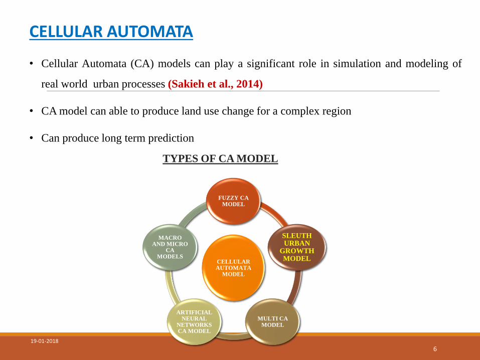
CELLULAR AUTOMATA
• Cellular Automata (CA) models can play a significant role in simulation and modeling of
real world urban processes (Sakieh et al., 2014)
• CA model can able to produce land use change for a complex region
• Can produce long term prediction
CELLULAR AUTOMATA
MODEL
FUZZY CA MODEL
SLEUTH URBAN
GROWTH MODEL
MULTI CA MODEL
ARTIFICIAL NEURAL
NETWORKS CA MODEL
MACRO AND MICRO
CA MODELS
TYPES OF CA MODEL

SLEUTH
19-01-2018
7
• SLOPE S
• LANDUSE L
• EXCLUSION E
• URBAN EXTENT U
• TRANSPORTATION T
• HILLSHADE H

Anushiya et al., 2015, studied the changes in water balance components of the
Chennai basin under present and future climate scenarios using Soil Water Assessment
Tool (SWAT).
Many studies have evaluated the effect of either urbanization (Chang 2007; Yang et
al., 2010) or climate changes (Woldeamlak et al., 2007; Sanchez G et al., 2009) on
watershed runoff;
The combined effects of these two effects using simulation models have been coming
under increased scrutiny in recent years ( Cuo et al., 2009; Srinivasan V et al., 2013).
19-01-2018 8
Combined Land use and climate change
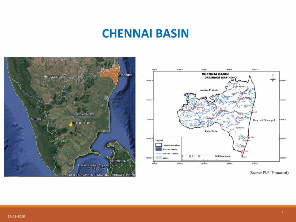
CHENNAI BASIN
19-01-2018
9
9

METHODOLOGY
19-01-2018 10
Identification of LANDSAT cloud free satellite imageries
Supervised classification using ERDAS IMAGINE
Landuse classified image 2000, 2008, 2010 qnd 2016
LULC change
Preparation of input layers (SLEUTH)
Slope – SRTM DEM (90 x90 m)
Landuse - Classified image from
LANDSAT (30 x30 m)
Excluded – Waterbodies from LULC
Urban extent – Built up area from LULC
Transportations – Open street maps
Hillsahde – DEM ( 90 x 90 m)
Calibration phase
Coarse , Fine and Final
Prediction phase
Projected LULC 2036
Hydrological modelling (SWAT)
LULC 2016
+
DEM
+
Soils from FAO
HRU
Weather data 2001 -2016
SWAT RUN
Hydrological components
LULC 2036
+
DEM
+
Soils from FAO
HRU
MIROC 3.2 A1B scenario
SWAT RUN
Hydrological components
Comparison between 2016 and 2036

FITTEST GLOBAL CLIMATE MODEL
RM
SD
CC
CM
A_
CG
CM
3.1
CN
RM
_C
M3
GF
DL
_
CM
2.0
MIR
OC
_3
.2
MR
I_C
GC
M
2.3
.2
MIU
B_
EC
HO
_G
_
MP
I_
EC
HA
M5
IPS
L_
CM
4
LE
AS
T O
F
RM
SE
T-M
AX
0.948 0.942 0.953 0.686 0.833 0.813 1.061 1.492 0.686
T-M
IN
1.862 1.817 1.654 1.633 1.819 1.852 1.882 2.136 1.633
PP
T
496.458 433.654 493.3 417.181 437.557 384.783 505.64 600.3 384.7

INFERENCES
1) Since there is an evident trend in T-Min and probable trend in T-Max, these two parameters are given priority in selecting the best GCM for the study area.
2) Also the model with highest possible resolution should be selected for greater degree of representation.
3) Hence MIROC_3.2 is chosen for climate change prediction.

MIROC_3.2
Model sponsored from Japan.
MIROC_3.2 (Model for Interdisciplinary Research on Climate)
Atmospheric Resolution: ◦ T106 ( 120 km * 120 km) and 60 vertical levels
Ocean Resolution: ◦ 0.28125 degree in longitude, 0.1875 degree in latitude, and 47
vertical levels

DATA SET USED
19-01-2018 14
S.NO DATA SOURCE
1 Slope DEM data
SRTM (90 x 90 m)
2 Land use map
LANDSAT image – (30 x 30 m )
OCT 2000- LANDSAT 7
MAY 2008- LANDSAT 5
OCT 2010- LANDSAT 5
MAY 2016- LANDSAT 8
3 Excluded layer Land use map - (30 x 30 m )
4 Urban extent layer Land use map - (30 x 30 m )
5 Transportation layer Open street view map
6 Hill shade layer DEM data-
SRTM (90 x 90 m )
7 Rainfall IMD
8 Soil map FAO
9 Climate data MIROC 3.2

Slope layer
19-01-2018 15
Slope Layer
A slope layer of the study area was
created from a Digital Elevation
Model (DEM) which was developed
from a SRTM-DEM ( 90 x 90 m)
image.
Slope value ranges from 2 to 80 % .
Mostly study area comes under flat
terrain category
INPUT LAYERS FOR SLEUTH MODEL

19-01-2018 16
Exclusion layer
Exclusion layer
The exclusion map was
created from the landuse layer.
The excluded areas have a
value of 1 and the areas
available for urban
development have a value of
0.
In this study water bodies are
considered as the excluded
areas.
INPUT LAYERS FOR SLEUTH MODEL

19-01-2018 17
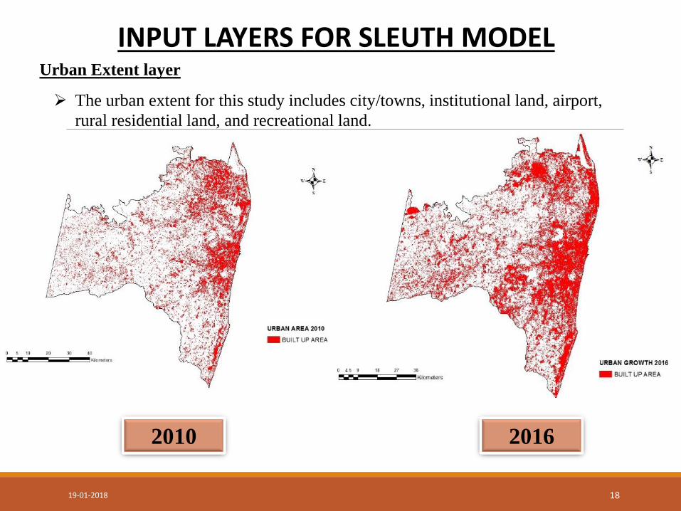
Urban Extent layer
The urban extent for this study includes city/towns, institutional land, airport,
rural residential land, and recreational land.
2000 2008
INPUT LAYERS FOR SLEUTH MODEL
19-01-2018 18
2010 2016
Urban Extent layer
INPUT LAYERS FOR SLEUTH MODEL
The urban extent for this study includes city/towns, institutional land, airport,
rural residential land, and recreational land.

19-01-2018 19
Transportation layer
Open street maps has been used to create road network maps of Chennai basin
2010 2016
INPUT LAYERS FOR SLEUTH MODEL

19-01-2018 20
Hillshade Layer
Hill shade is a shaded relief
on a map, just to indicate
relative slopes, mountain
ridges, not absolute height.
Hill shade was created using
SRTM – DEM ( 90 x 90 m)
INPUT LAYERS FOR SLEUTH MODEL
19-01-2018 21
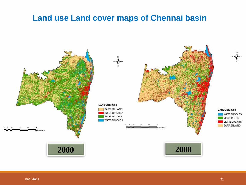
Land use Land cover maps of Chennai basin
2000 2008

19-01-2018 22
Land use Land cover maps of Chennai basin
2016 2010
Land use Land cover maps of Chennai basin

LULC changes were estimated for the years 2000, 2008, 2010 and 2016 using
LANDSAT series satellite imageries
Supervised classification of the imageries were performed using maximum
likelihood algorithm in ERDAS Imagine.
Vegetation, Barren land, Built up area and Water bodies are the Land use Land
cover classes used for the classification
Reason for the LULC changes may be attributed to rapid population growth,
rural to urban migration, poverty and reclassification of rural to urban areas.
It was found that some of the agricultural lands in the North West part of the basin
was rapidly changing to built-up areas due to urbanization
19-01-2018 23
Land use Land cover Change

CATEGORY
(5474.89 km2)
Land use and Land cover
km2 %
2000
(Base Year) 2008 2010 2016 2008 2010 2016
Barren Land 2048.40 3062.40 2399.15 1668.01 49.51 17.14 -18.54
Vegetation 2568.20 1077.14 1574.19 1472.06 -58.04 -73.72 -42.68
Built Up Area 468.14 991.22 1310.38 2134.20 111.74 179.8 355.87
Waterbodies 390.14 342.12 189.16 199.61 -12.13 -51.4 -48.75
19-01-2018 24
Land use Land cover Change

Considering the year 2000 as base year, Table 1 shows that there is rapid increase in
the built up area class.
Vegetation and Water bodies have decreased considerably over the past decade.
Built up area comprising human habitations developed for non-agricultural uses like
building, transport and communications is largely broadened from 468.14 km2
(2000) to 2134.20 km2 (2016).
This is due to urban expansion and population increase in the study area.
For instance vegetation has been greatly decreased from 2568.20 km2 to 1472.06
km2 between 2000 and 2016 with the net decline of 42.68 % (Table 1).
19-01-2018 25
Land use Land cover Change

Another interesting observation in the basin is that a significant amount of agricultural
land is converted into settlements and other urban developmental activities.
Water spread area both manmade and natural water features such as rivers, tanks and
reservoirs were also decreased from 390.14 km2 (2000) to 199.61 km2 (2016) with a
decrease of 48.75 % (Table 1).
Water spread area decrease is attributed to the fact that there is a gradual conversion of
water spread area into built up area by encroachments.
Barren land initially increased for few years from 2048.40 km2 (2000) to 3062.40 km2
(2008) and then gradually decreased to 1668.8 km2 in 2016 (Table 1).
19-01-2018 26
Land use Land cover Change

Urban Growth Model (SLEUTH) Calibration
The model runs in three modes; test mode, calibration mode and the prediction
mode.
In test mode data is tested for readiness of calibration and prediction.
Calibration phase is done to determine the best fit values for the five growth control
parameters including coefficients of diffusion, breed and spread, slope resistance
and road gravity with historical urban extent data.
Lee Sallee metric helps to select the values for the next phase of calibration is used
in this study.
19-01-2018 27

Test mode has been done for the historic data (Land use Land Cover maps 2000,
2008, 2010 and 2016) by taking the best fit coefficients values given in Table 2 with
Four Monte Carlo Iterations
Coarse calibration for predicting 2036 sprawl using the past data has been performed
by taking a start value of 0, step value of 25 and stop value of 100 with four Monte
Carlo iterations of 3125 simulations.
Similarly fine and final calibration has been done by taking the coefficients from
pervious phase with the Monte Carlo Iteration of Six and Eight respectively
19-01-2018 28
Urban Growth Model (SLEUTH)

Monte Carlo Iterations are set to 100 and best fit values for prediction are given in
following table.
The urban expansion in Chennai basin is a mixture of Breed, spread and road
gravity expansion.
Breed has best fit value of 100 which shows very high scope of new settlements
being generated.
19-01-2018 29
S.No Prediction Coefficient Best Fit
Value
1 Prediction Diffusion Best Fit 1
2 Prediction Breed Best Fit 100
3 Prediction Spread Best Fit 12
4 Prediction Slope Best Fit 1
5 Prediction Road Best Fit 85
6 Prediction Start Year 2016
7 Prediction Stop Year 2036
8 Mount Carlo Iterations 100
Urban Growth Predictions

19-01-2018 30
S.NO Year Urban Area
km2
1 2016 2134.65
2 2036 3415.99
Simulated Urban growth of Chennai basin using SLEUTH 2016 and 2036
2016 2036

19-01-2018 31
Urban Growth Predictions Using Sleuth Model

S.No Sub Basin Name Area
km2
Urban Area
in 2016
km2
Urban Area
in 2036
km2
Difference
in urban area
Percentage
increase with
respect to area
Percentage
increase with
respect to 2016
1 Pulicat 589.79 293.60 383.07 89.47 65 30
2 Arniar 488.42 157.00 289.49 132.49 59 84
3 Kortalaiya 1117.51 392.48 697.06 304.58 62 77
4 Nagari 954.28 356.70 595.00 238.30 62 67
5 Mandi 978.70 198.85 465.10 266.25 56 134
6 Adyar 702.90 343.50 463.00 119.50 66 34
7 Upper Palar 800.70 391.08 521.50 130.42 65 33
19-01-2018 32
Urban Growth in Sub basin Level
0
100
200
300
400
500
600
700
800
Pulicat Arniar Kortalaiya Nagari Mandi Adyar Upper Palar
1 2 3 4 5 6 7
Are
a , k
m2
URBAN AREA IN 2016 URBAN AREA IN 2036

SIMULATION RESULTS OF SLEUTH
Results of the percentage increase in the urban extent at subbasin level indicates urbanization
will happen as new spreading centre growth.
Therefore it is necessary to understand the impact of these urban extent growth on the
availability of water resources in the future for better management and planning.
Hence for further analysis it was decided to study at a selected subbasin of the Chennai basin.
Since Adyar subbasin has experienced floods in the year 2015, it was decided to
implement the hydrological model (SWAT) at Adyar sub basin to assess the impact of
predicted urban growth (2036) under AIB scenario of the IPCC using MIROC 3.2,
CMIP3 model data.
19-01-2018 33

SWAT Model
Adyar subbasin area was subdivided into 47 sub watersheds.
The land use map of Adyar sub basin was classified for the year 2016 and for 2036
the projected land use maps from SLEUTH urban growth model was used.
19-01-2018 34
Sub basin map
3 years warm up period.
Soil map from the Food and
Agriculture Organization of the
United Nations (FAO, 1995).
175 HRU

Water Balance of Adyar sub basin in 2016 and 2036
19-01-2018 35
Water balance of Adyar subbasin in 2016 Water balance of Adyar subbasin in 2036

19-01-2018 36
Annual average Evapotranspiration for 2016 and 2036
2016 2036
Evapotranspiration Rate
The maximum evapotranspiration rate has a reduction from 1180 mm to 866 mm.

19-01-2018 37
2016 2036
Annual average Groundwater flow for 2016 and 2036
Groundwater Flow
The minimum range of Groundwater is 50mm in 2016 is reduced by 50% in the year 2036.

19-01-2018 38
2016 2036
Annual average Percolation rate for 2016 and 2036
Percolation
The percolation component has reduced to 122 mm (2036) from 144 mm in 2016

19-01-2018 39
2016 2036
Annual average Surface runoff for 2016 and 2036
Surface Runoff
The Runoff component has more impact due to the urbanization. The model predicts that the
minimum runoff value has increased from 450 to 700 mm

19-01-2018 40
Annual average Soil water for 2016 and 2036
2016 2036
Soil Water
The soil water component has a maximum reduction from 4382 mm to 750 mm. This
decrease in soil water depicts the reduction in groundwater component too

19-01-2018 41
Annual average Water yield for the 2016 and 2036
2016 2036
Water Yield
The increasing surface runoff has led to the increase in water yield in the year 2036.
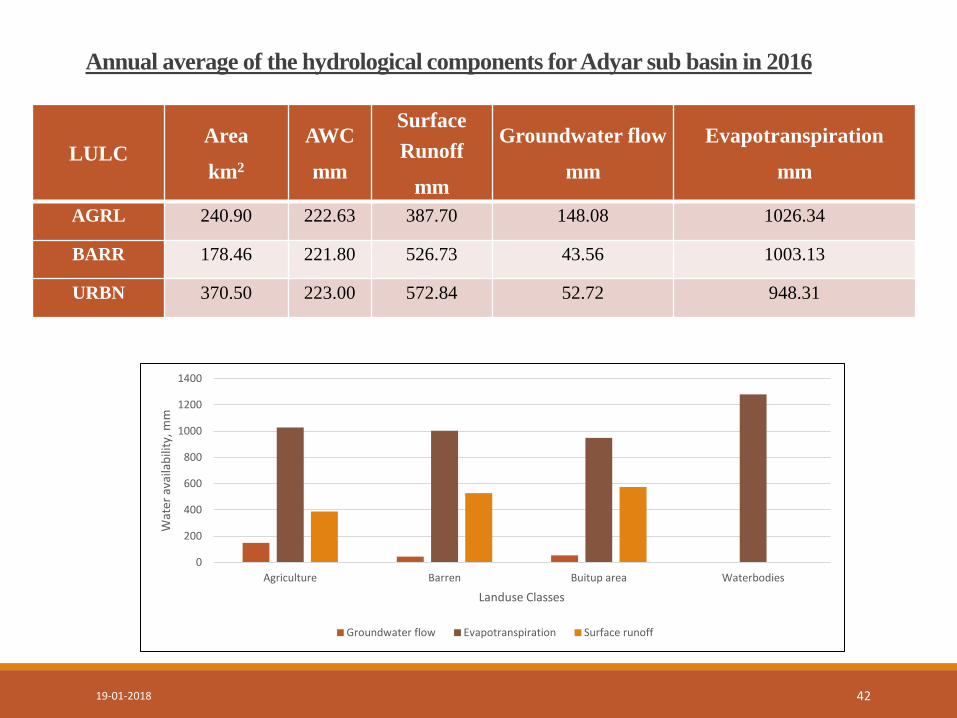
Annual average of the hydrological components for Adyar sub basin in 2016
LULC Area
km2
AWC
mm
Surface
Runoff
mm
Groundwater flow
mm
Evapotranspiration
mm
AGRL 240.90 222.63 387.70 148.08 1026.34
BARR 178.46 221.80 526.73 43.56 1003.13
URBN 370.50 223.00 572.84 52.72 948.31
19-01-2018 42
0
200
400
600
800
1000
1200
1400
Agriculture Barren Buitup area Waterbodies
Wat
er a
vaila
bili
ty, m
m
Landuse Classes
Groundwater flow Evapotranspiration Surface runoff
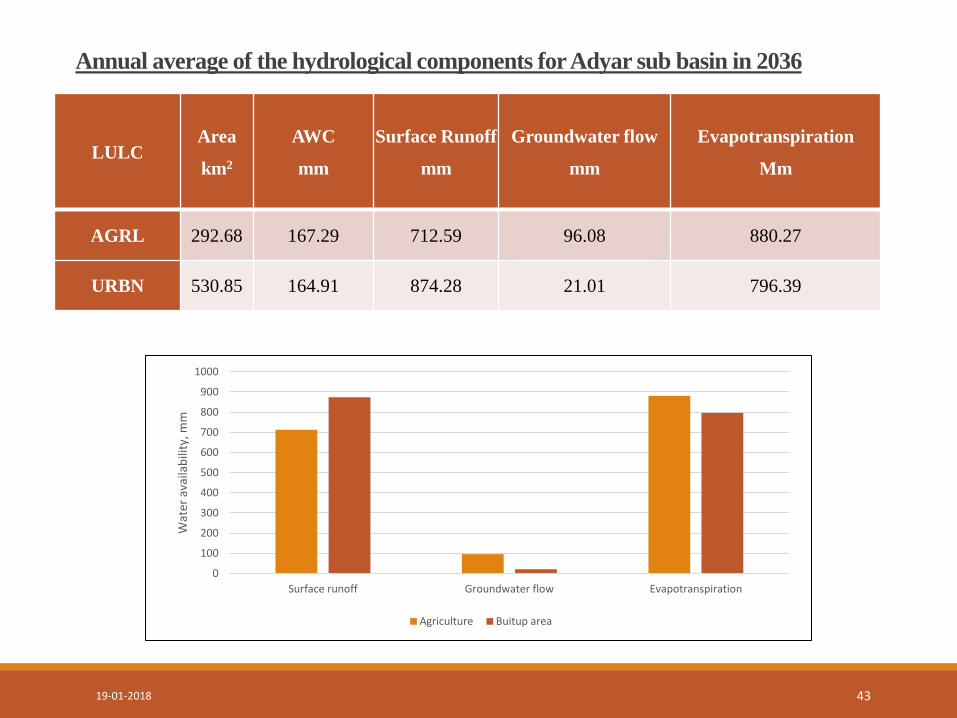
Annual average of the hydrological components for Adyar sub basin in 2036
LULC Area
km2
AWC
mm
Surface Runoff
mm
Groundwater flow
mm
Evapotranspiration
Mm
AGRL 292.68 167.29 712.59 96.08 880.27
URBN 530.85 164.91 874.28 21.01 796.39
19-01-2018 43
0
100
200
300
400
500
600
700
800
900
1000
Surface runoff Groundwater flow Evapotranspiration
Wat
er a
vaila
bili
ty, m
m
Agriculture Buitup area

Impact of urban growth on hydrological components for the year 2016 and 2036
0
100
200
300
400
500
600
700
800
900
1000
2016 2036
Wat
er a
vaila
bili
ty,
mm
Year
Surface runoff Groundwater flow Evapotranspiration
19-01-2018 44
S. No Urban area Surface runoff
mm
Groundwater flow
mm
Evapotranspiration
mm
1 2016 572.84 52.72 948.31
2 2036 874.28 21.01 796.39

Summary
The urban growth model simulations have shown a significant increase in the
urban extent from 2134.65 km2 (2016) to 3415.99 km2 (2036) for Chennai basin.
The urban expansion is mainly by breed coefficients with the value of 100
because of new spreading area and is not resisted by slope.
The study was further carried on to assess the impact of climate change on
hydrological components like surface flow, potential evapotranspiration using
SWAT
19-01-2018 45

The future climate data was obtained from the global climate model, MIROC 3.2.
This model was selected to extract the future climate data for the A1B future scenario.
Since Adyar subbasin has experienced floods in the year 2015, it was decided to
implement the hydrological model (SWAT) at Adyar subbasin.
The results revealed that the Runoff component has more impact due to the
urbanization.
The model predicts that the minimum runoff value has increased from 450 to 700 mm.
19-01-2018 46
Summary
The maximum evapotranspiration rate has a reduction from 1180 mm to
866 mm.
The study concludes that the water resources of Chennai basin will suffer
under the projected urban growth and climate change .
The impacts are very significant in the hydrological component especially
run off.
19-01-2018 47
Summary

River discharge measurement

River discharge measurement

Hydrograph of Adyar river at Kotturpuram bridge

REFERENCES 1. Anushiya J and Ramachandran A (2015), ‘Assessment of Water Availability in Chennai
Basin under Present and Future Climate Scenarios’, Springer Earth System Science,pp.397-415.
2. Bharath and Ramachandra T V (2015), ‘Visualization of Urban Growth Pattern in Chennai using Geoinformatics and Spatial Metrics’, Indian Society of Remote Sensing.
3. Bihamta N, Alireza S, Sima F and Mehdi G (2015), ‘Using the SLEUTH Urban Growth Model to Simulate Future Urban Expansion of the Isfahan Metropolitan Area, Iran’, Indian Society of Remote Sensing,pp.407–414 .
4. Chang H (2007), ‘Comparative stream flow characteristics in urbanizing basins in the Portland Metropolitan Area, Oregon, USA’, Hydrological Processes, pp. 211–222.
5. Changlin Y, Dingquan Y, Honghui Z, Shengjing Y and Guanghui C (2008), ‘Simulation of urban growth using a cellular automata-based model in a developing nation’s region’, Geoinformatics 2008 and Joint Conference on GIS and Built Environment.
19-01-2018 51

REFERENCES
6. Clarke K and Gaydos L (1998), ‘Loose-coupling a cellular automaton model and GIS, long-term urban growth prediction for San Francisco and Washington Baltimore’, International Journal of Geographical Information Science, pp.699–714.
7. Cuo L, Lettenmaier D P, Alberti M and Richey JE (2009), ‘Effects of a century of land cover and climate change on the hydrology of the Puget Sound basin’, Hydrological Processes, pp. 907–933.
8. Faramarzi M, Abbaspour K, Schulin R and Yang H (2009), ‘Modelling blue and green water resources availability in Iran’, Hydrological Process, vol. 23, pp.486–501.
9. Glavan M, Pintar M and Volk M (2012), ‘Land use change in a 200-year period and its effect on blue and green water flow in two Slovenian Mediterranean catchments—lessons for the future’, Hydrological Process pp.1-18.
10. Hakan O,Hakan D ,Birsen K and Engin N(2011), ‘Modeling Urban Growth and Land Use/Land Cover Change in Bornova District of Izmir Metropolitan Area From 2009 to 2040’, International Symposium on Environmental Protection and Planning: Geographic Information Systems (GIS) and Remote Sensing (RS) Applications (ISEPP).
19-01-2018 52

THANK YOU
19-01-2018 53