International Master’s Thesis

Integrating the use of prior information into Graph-SLAM with NDTregistration for loop detection

Antek SchabertÖrebro University, Sweden

Technology

örebro 2017

Integrating the use of prior information into Graph-SLAM with NDTregistration for loop detection

Antek SchabertÖrebro University, Sweden

Integrating the use of prior information intoGraph-SLAM with NDT registration for loop

detection

© Antek SchabertÖrebro University, Sweden, 2017

Title: Integrating the use of prior information into Graph-SLAM with NDT registration for loopdetection

Contents

1 Introduction 9

2 Related Work 11

3 Normal Distribution Transform 15

4 Graph-Based SLAM 19

5 Probabilistic Motion Models 21

6 Optimization 23

7 Prior information 27

8 Localization 33

9 Results 359.1 Test setup . . . . . . . . . . . . . . . . . . . . . . . . . . . . . . . . 359.2 Simulation results . . . . . . . . . . . . . . . . . . . . . . . . . . . . 37

10 Conclusions 41

7

Chapter 1

Introduction

With the increased use of autonomous agents in open and often changing environmentsit is important that these agents have the ability to accurately localize themselves intheir environment and build a map of the environment. If global localization systemssuch as GPS are not available or are not accurate enough, agents often have to relyon range sensors and odometry information for localization. Building a map and atthe same time using the map for localization is known as simultaneous localizationand mapping (SLAM) and is one of the most important problems in robotics. It isnecessary for an efficient solution to many other problems, such as path planning andmulti-agent coordination. Most SLAM approaches maintain an uncertainty estimationof the position of the agent and try to detect features in the map that were detected pre-viously to reduce this uncertainty and improve the position estimation and, therefore,also the map quality.

Although several techniques for SLAM exist, they are still not mature enough foruse on heavy production vehicles. As an effort to improve reliability of a mapping andlocalization system, one direction of research is the use of prior information. If a robotsystem could exploit prior information - in the form of, e.g., aerial or satellite images,CAD drawings, or hand-drawn sketches - it should be able to build a detailed localmap using its own sensors more quickly and more accurately. However, matchinginformation from such a rough map (which may be out of date, or using differentfeatures compared to what the robot can directly observe) to the robots observationsis a non-trivial task.

In this paper an algorithm will be presented that combines Graph-SLAM with poseestimates extracted from running MCL on a prior map. However, unlike in other pa-pers only radar sensors will be used as input. Since radar sensors are allowed for useon public streets in most parts of the world this makes the results of this paper widelyuseable. On the other hand radar sensors generally provide less data from the environ-ment and more noise than 2D laser range finders. To handle this noise and minimizethe error introduced by it NDT (Normal Distribution Transform) scan registration willbe used for loop detection.

9

Chapter 2

Related Work

While the research focus on SLAM algorithms has generally improved the qualityof the generated maps in comparison to the results of widely used algorithms from20 years ago. But at the same time the diversity of possible algorithms with their ownstrengths and drawbacks makes the decision which algorithm to use more complicated.This is in our case even more so, since most algorithms are defined without additionalinformation sources in mind and the work to extend the algorithms to accept suchinput has to be estimated as well as the type of information that could be used. Inthis chapter we will give an overview of the currently common SLAM algorithmsand give a quick opinion about how additional information may be introduced to thealgorithms. Since the SLAM problem is closely related to the localization problemit is not surprising that many approaches to the problem follow a similar idea as thelocalization algorithms Monte Carlo Localization and the Extended Kalman Filter.

Particle based algorithms similar to the one presented by Montemerlo et al. [1]generate a multi-hypothesis system where the agent draws a different sample from themotion model for each hypothesis and builds a map for each hypothesis as well. Thisworks well if the agent often moves back into already mapped areas where inaccurateparticles can be discarded. While prior information could be used to run the local-ization step on the prior map as well and particles could be discarded according to amixture of the weight of the localization on the prior map and the local map, the bestparticle might be discarded to fit outdated information and it would be impossible torecover this information once we reach an area that was already mapped again.

On the other hand solutions to the SLAM problem that use the extended Kalmanfilter [2] or the sparse extended information filter [3] for the localization make strongassumptions about the motion model and the sensor noise. If these assumptions do notrepresent the reality, the errors from the approximation will accumulate and eventuallylead to inconsistencies [4]. If the positions of landmarks were given on a prior map orcould be calculated these known locations could be used as an initial estimate for thelandmarks. This would directly improve the uncertainty of the filter when a landmarkis detected for the first time.

In contrast Lu and Milios proposed to keep all scans of the environment togetherwith relations between different poses and the covariance matrix of those relations inmemory [5]. The relations can, for example, be derived from the odometry or scanmatching. Finally, they propose to use least squares optimization to find the mostlikely poses of the agent. This representation is now commonly known as Graph-BasedSLAM or Graph-SLAM. While this allows to correct errors made in the mapping, thecomputational complexity being O(n3) in relation to the poses n made this approachonly practical for problems with few poses. However, since then, more efficient algo-rithms for the optimization problem were presented and are now easily available [6].This allows the use of Graph-Based SLAM also on problems with many more poses.Prior information can easily be introduced as fixed points in relation to an agent pose.

11

12 CHAPTER 2. RELATED WORK

The uncertainty of the prior information is then used for the covariance or informationmatrix of the relation.

Aside from particle based approaches that only measure the likelihood of a scan,given the map of the particle, all these algorithms rely either on landmark or loopdetection to reduce the error in the estimated pose of the agent. In both cases thecore of the problem is often to match two scans to find the relative pose between thepositions where the scans were taken. This is known as scan registration and can bedivided into two categories - local search strategies and global search strategies. Localsearch strategies require a good initial guess of the relative pose and easily get stuckin local minima if the guess is too far off from the correct pose.

A straightforward approach in this category is to find for every point in one scanthe closest point in the other scan and minimize the distance as proposed by Besl [7].This is commonly known as the iterative closest point (ICP) algorithm and is probablythe most widely used solution to scan registration. The biggest drawback of it is thatthe search for the closest point is quite time consuming. While this problem can bereduced by storing the points in a semi-organized form and sampling in dense areas, adifferent representations of the point clouds can avoid it altogether.

In the Normal Distribution Transform (NDT) [8] a point cloud is represented by acollection of local normal distributions, where each normal distribution represents thelikelihood distribution of a point falling into a certain area. These normal distributionsare typically ordered in a grid or an N-tree structure, so that finding the closest normaldistribution for a point is a simple lookup operation or search of the neighboring cellsif the initial cell was empty, instead of iterating over a whole point cloud. In addi-tion, normal distributions have analytic derivatives, which allows the use of standardoptimization methods for the registration process.

Another approach from Stoyanov et al. converts both, the reference and the reg-istration point cloud, into an NDT representation and minimizes the L2 distance be-tween the NDT maps [9]. While this leads in many cases to faster computation timesunlike regular NDT registration this approach has, assuming that both NDT maps havethe same amount of cells, a quadratic computational complexity in regard to the num-ber of cells of the NDT maps. This makes the choice of the cell size a more importantfactor and works better for the registration of two independent scans rather than reg-istration of a scan to a map.

On the other hand global search strategies do not rely on an initial guess, but rathersearch over all possible transformations. Since this is very time expensive, strategiesoften include additional discretization [10] or using local feature descriptors that arerotation invariant [11] to reduce the search space.

Including information from prior maps into the SLAM process is a rather newresearch area and there are two important factors that have to be considered. First wecan not assume that the map is accurate, since it was most likely taken at a differenttime and it might lack details depending on how it was created. Second the map mightinclude different information depending on the sensor that was used to create the mapand the vantage point of the sensor, or if the map was created by a sensor at all.Kümmerle et al. show how localization on prior information can be used to improvethe accuracy of a SLAM algorithm [12], but does not consider inaccuracies of the map.Closely related Vysotska and Stachniss [13] use Open Street Maps to bound the errorof Graph-SLAM, but use ICP registration instead of MCL to extract the informationfrom the prior map. Parsley et al. propose to use prior information as bounds for thelocation of landmarks instead of influencing the pose of the agent directly [14]. Whileall these publications use laser range finders we will be using radar sensors, which arealready used in many modern vehicles for parking assistants, collision avoidance andother driving assistence systems. In contrast to laser range finders radars have a lotless valid detections, may detect occluded objects, don’t have a fixed angle differencebetween detections and more noise than laser range finders.

13

On the other hand, including prior information about the structures in the envi-ronment can especially improve rotational uncertainties. For example, Newman et al.proposed to search for line features that are almost parallel or orthogonal and addartificial observations to make these features fully parallel or orthogonal [15].

In his doctoral work Parsley also discussed the integration of different informationof observed features, but the used information is generated by hand rather than from amap [16].

Chapter 3

Normal Distribution

Transform

Scan registration is the process of finding an affine transformation function that projectsthe sensor readings of one time-frame onto the sensor readings of another time-frameand minimizing the difference between the two scenes. It is used in various areas inrobotics and also other research fields. For example it can be used to provide accurateestimations of the odometry, recognize loops in SLAM algorithms and detect movingobjects. The result of a NDT scan registration can be seen in Figure 3.1.

Figure 3.1: Results of a NDT scan registration. Black is the reference map, red is the initialguess of the scan and blue the result after scan registration

However, sensor readings are often acquired in the form of point clouds whichcontain a lot of redundant information - the points are mostly samples from sur-faces the sensor detected. While most registration algorithms work directly on thesepoint clouds, this is a computation heavy process and does not take advantage of anyinformation about the surface itself. Biber and Straßer [8] proposed to divide two-dimensional point clouds into cells and calculate a normal distribution for every cell.These normal distributions now approximate the local surface, from which the points

15

16 CHAPTER 3. NORMAL DISTRIBUTION TRANSFORM

were sampled, and provide smooth gradients, the orientation of the surface, as well asthe probability of a point being sampled from the corresponding normal distributionin a certain position. While the whole map now is represented as a Gaussian mixturemodel of the normal distributions, the normal distribution of a cell alone provides agood enough local approximation over the area of the cell and the error of calculatingthe probability of a point falling into the cell without using the normal distributions ofthe rest of the map is insignificant. This can be assumed since all normal distributionswere calculated using only points inside the cell and, therefore, have their mean insidethe cell and a covariance matrix that does not overlap much with other cells.

In more detail the equation 3.1 now provides for every point x an easy way to cal-culate the probability that the point was generated by the same structure that generatedthe points used for the normal distribution.

p(x) =1

(2π)D/2√|Σ|

exp(− (x−µ)T Σ−1(x−µ)

2

)(3.1)

with the mean

µ =1n

n

∑k=1

xk, (3.2)

the covariance

Σ =1

n−1

n

∑k=1

(xk−µ)(xk−µ)T (3.3)

and the dimension D.With a probability for each point we can now define the optimal transformation of

the point cloud as the one that maximizes the product of the probabilities of the points[17].

ψ =n

∏k=1

p(T (p,xk)) (3.4)

where T (p,xk) is the transformation function applied to the point xk.However, with this equation single outliers would have a strong impact on the

resulting transformation. To avoid such a behavior it is common to use a mixture of anormal distribution and a uniform distribution.

p(x) = c1 exp(− (x−µ)T Σ−1(x−µ)

2

)+ c2 po (3.5)

where the constants c1 and c2 can be calculated by applying the requirement that theintegral of the normal distribution over the cell has to be one and po is the expectedrate of outliers.

It is also common in optimization problems to minimize a score function insteadof maximizing it. Also, by taking the logarithm of the probabilities the product can beturned into a sum. This way, the derivative of the resulting function

− logψ =−n

∑k=1

log p(T (p,xk)). (3.6)

can now be calculated for each summand independently. While this score function isrobust to outliers the derivatives of a logarithm are typically not fully defined. Biberalso proposed to approximate the logarithm of a probability with a new Gaussianfunction [8].

17

d3 =− log(c2)

d1 =− log(c1 + c2)−d3

d2 =−2log((− log(c1 exp(−1/2)+ c2)−d3)/d1)

(3.7)

p(x) =−d1 exp(−d2

2(x−µ)T

Σ−1(x−µ)

)(3.8)

This approximation provides the same characteristics for optimization but has simplerderivatives if used for the score function

s(p) =−n

∑k=1

p(T (p,xk)). (3.9)

Newton’s algorithm is a well known optimization algorithm that iteratively solves theequation

H∆p =−g (3.10)

where H is the Hessian matrix and g is the gradient vector of s(p). The result ∆pis then added after each step to the transformation vector p. The gradient vector andthe Hessian matrix can be derived by calculating the first and second order partialderivatives of s(p) respective to the coefficients of p. The entries of the gradient vectorare

gi =δ sδ pi

=n

∑k=1

d1d2x′kT

Σ−1k

δx′kδ pi

exp(−d2

2x′k

TΣ−1k x′k

)(3.11)

where x′k = T (p,xk)−µk. µ as well as Σ now have subscripts to indicate that they aretaken from the cell the point xk falls into after being transformed by p. In a similarfashion the equation for the entries of the Hessian matrix are

Hi j =δ 2s

δ piδ p j=

n

∑k=1

d1d2 exp(−d2

2x′k

TΣ−1k x′k

)(−d2

(x′k

TΣ−1k

δx′kδ pi

)(x′k

TΣ−1k

δx′kδ p j

)+ x′k

TΣ−1k

δ 2x′kδ piδ p j

+

(δx′kδ p j

)T

Σ−1k

δx′kδ pi

).

(3.12)

While these equations may look complex the computational complexity is O(n+m)with n being the number of points in the scan to be matched and m being the numberof points in the scan used for the normal distributions. This is easy to see since allequations used here are scaling linearly with the number of points. The only other taskwe need to perform is to pool the points of the point cloud used for the NDT cells intotheir respective cells. Since the corresponding cells can be found by a simple look-upaction this only takes linear time as well if a data structure with linear computationalcomplexity is used to store the points for each cell.

In comparison ICP has a complexity of O(n ∗m). While the idea behind ICP isquite simple, the algorithm has to search for each point in the point cloud for its near-est neighbor in the fixed point cloud. Without optimization this has a computationalcomplexity of O(n∗m). While this runtime can be reduced in average, by pooling thepoints before the matching, the worst case still stays O(n∗m).

This makes NDT scan registration on dense point clouds a lot faster. On the otherhand it can also improve the accuracy of the result if the used sensors are subject to alot of white noise.

We will be using NDT scan registration in this work. While our sensor data isnot very dense our sensors are subject to a lot of noise. While ICP would also work,

18 CHAPTER 3. NORMAL DISTRIBUTION TRANSFORM

the results would be influenced more by the initial guess. For example if we tried toregister 2 scans of a wall ICP would probably, depending on which side of the wall theinitial guess started, end a bit away from the actual mean to the side it started from.

Chapter 4

Graph-Based SLAM

One of the central problems in robotics is the building of a map of an unknown en-vironment by only using the data of on-board sensors. This problem is known as si-multaneous localization and mapping or in short SLAM. This process is complicatedsince the measurements of sensors are subject to many noise sources. Without correct-ing these errors the uncertainty of the real pose of the robot will increase over timeand make a consistent alignment of the range measurements impossible.

Many different approaches to this problem were published in the past. Most ofthem calculate the current pose from the last pose and the odometry readings directlyand keep track of the uncertainty of this pose in another way. When additional in-formation, e.g. through loop or landmark detection, the current pose is recalculatedfrom the likelihood fields of the new information and the uncertainty around the pose.However in most cases neither old poses nor the map built from these old poses iscorrected.

Graph-Based SLAM on the other hand is keeping all scans, poses, relative infor-mation between poses and the uncertainty of the relative information in memory anduses optimization algorithms to correct not only the current pose but also all past posesof the robot. The representation used here can be described as a directed graph. Thebest estimations for the poses of the robot are stored in the nodes. The edges in thegraph on the other side store a probability distribution of the relative movement orobservation from one pose to another. This information is generally represented asa vector of the special Euclidean group 2 and a covariance or information matrix ofa normal distribution. The mean value of the normal distribution is not stored sepa-rately since it is considered to be the movement or observation vector. When the graphis build the edges are, for example, set to the odometry readings and the probabilitydistribution according to the motion model. The initial pose of the nodes is then de-termined by assuming that the robot performed the movement stored in the edge fromthe pose of the last node in the graph. However, once enough observations are addedto the graph these poses will iteratively be changed by minimizing an error functionof the edges.

To perform such an optimization it is necessary to have a fixed anchor point inthe graph and additional edges aside from the odometry readings. The anchor pointis generally assumed to be the first node, which will not be optimized. While theactual pose of this node is not relevant, it is generally assumed to be the origin of thecoordinate system.

Additional edges are typically generated by performing scan registration or land-mark detection. Figure 4.1 shows how a Graph with such information may look like.

Scan registration is typically performed by matching the current scan to scans ofother poses that are assumed to be close enough to provide a good initial guess. Theresulting transformation vector is then added as a new edge to the graph between thetwo scans. Calculating a plausible information matrix for the edge on the other hand is

19

20 CHAPTER 4. GRAPH-BASED SLAM

Figure 4.1: Graph-SLAM

a more complicated problem and depends on the scan registration algorithm that wasused. If ICP was used a covariance matrix may be calculated from the points of thecurrent scan and the corresponding closest neighbor points. The information matrix isthen simply the inverse of the covariance matrix. If NDT scan registration was usedthe Hessian matrix can be used as an estimate for the information matrix. However, inmost cases these matrices are inaccurate estimations of the true error. Especially if thealgorithm finds a local minimum the information matrix will not represent the errorcaused by this.

Landmark detection on the other hand extracts features from the current scan andadds a new edge between the current pose and a node that represents the feature. Sim-ilar to scan registration the information matrix of the edges is considered to representthe error from the sensors and the algorithm used to detect the feature. False detectionof landmarks will generally lead to large inaccuracies in the map. Landmark detectionwill not be used in the algorithm presented in this paper, since the main focus of thiswork is to include prior information into Graph-SLAM. While prior information alonewould be insufficient for good results, loop detection was simpler to implement and al-ready provides good results. Landmark detection on the other hand would most likelynot find unique features with the sparse data from the radar sensors and make match-ing the feature depending on the estimated pose necessary. How landmark detectionwould be used in Graph-SLAM is mainly included here for completeness.

In scan registration as well as landmark detection the problem of false positivescan be seen as a simple outlier problem. During optimization a false constraint willadd a large error to the nodes it is connected to and therefore change the pose of thesenodes. This error will then propagate throughout the whole graph. While the commonway to handle outliers would be to use a probability distribution model that limits theinfluence a single point can have on the complete probability we have to consider thatthe graph used for Graph-SLAM is in most cases sparse. This means the nodes havevery few constraints and even with a different probability model a wrong constraintcould still have a strong negative impact during optimization. Instead the common ap-proaches to this problem are to find the constraints, which add an unproportional largeamount to the total error of the graph and use switchable constraints [18], which maybe deactivated by the optimization algorithm or to allow the optimization algorithm toscale the covariance of outliers to reduce their influence on the graph [19].

Chapter 5

Probabilistic Motion

Models

In the last chapter we introduced that the edges of the graph in Graph-SLAM store theodometry readings and the corresponding information matrix. However, to provide aplausible information matrix we need to have a model of the motion and the noise ofthe sensors measuring the motion.

Figure 5.1: Thrun motion model [20]

The most common model was described by Thrun et al. in [21] and describes themotion of the robot over a short time frame as a rotation before the motion, a straightmotion and a rotation after the motion. Figure 5.1 shows how such a motion looks like.These three components are then considered to be subject to noise from the sensors.

δtrans = δtrans + εtrans εtrans ∼N (0,σ2trans)

δrot1 = δrot1 + εrot1 εrot1 ∼N (0,σ2rot1)

δrot2 = δrot2 + εrot2 εrot2 ∼N (0,σ2rot2)

(5.1)

The error of the motion is modeled as normal distributions around these three com-ponents of the motion. However, the standard deviations of the normal distributionsdepend on the length of the movement and the absolute of the rotations.

σrot1 = α1|δrot1|+α2δtransσtrans = α3δtrans +α4(|δrot1|+ |δrot2|)σrot2 = α1|δrot2|+α2δtrans

(5.2)

21

22 CHAPTER 5. PROBABILISTIC MOTION MODELS

α1 to α4 are the parameters that have to be tuned to fit the accuracy of the sensorsmeasuring the motion.

Due to the noise of the rotation before the motion the probability distribution afterthe motion takes on a bent form if projected to a plane only showing the positionwithout the angle and it is not possible to describe it with a normal distribution ingeneral.

However, if the noise to the rotation is rather low, a normal distribution providesa good approximation. In this case the Gaussian probabilistic motion model may beused. Here the motion is represented as a typical vector of the special Euclidean group2 or in short as a SE2 vector. The components of this vector are a forward part of themotion, a lateral part of the motion and a rotation after the motion. Once again thenoise is added onto these components

∆odox = ∆odo

x + εodox εodo

x ∼N (0,σ2∆odo

x)

∆odoy = ∆odo

y + εodoy εodo

y ∼N (0,σ2∆odo

y)

∆odoφ

= ∆odoφ

+ εodoφ

εodoφ∼N (0,σ2

∆odoφ

)

(5.3)

and the noise depends on the length of the motion and the rotation.

σ∆odo

x= σ

∆odoy

= σminxy +α1

√(∆odo

x )2 +(∆odoy )2 +α2|∆odo

φ|

σ∆odo

φ

= σminφ

+α3

√(∆odo

x )2 +(∆odoy )2 +α4|∆odo

φ|

(5.4)

While this model is theoretically less accurate, in practical use the rotation af-ter the motion may also represent the rotation before the motion of the next node inGraph-SLAM. This leaves the first edge without a rotation before the motion, but inGraph-SLAM the first pose is in general an arbitrary pose, which is fixed and simplyrepresents the beginning of the map. As such, unrepresented errors in the first pose donot affect our algorithm and can be ignored.

On the other hand this model is easier to integrate into Graph-SLAM and also pro-vides a better way to model position errors from other effects than rotational uncer-tainty. We will be using the Gaussian probabilistic motion model in this work. How-ever, we assume both motion models would provide a viable foundation for Graph-SLAM and later on localization on the prior map.

Figure 5.2: Gaussian probabilistic motion model [20]

Chapter 6

Optimization

In the chapter about Graph-SLAM we touched the topic of optimizing the graph as partof the algorithm. Since we already explained how Newton’s algorithm can be used tooptimize the score function during scan registration with NDT maps one might expectthat the score function

F(x) = ∑(i, j)∈C

Fi j(x) = ∑(i, j)∈C

e(xi,x j,zi j)T

Ωi je(xi,x j,zi j) (6.1)

of the graph may be minimized in the same manner. zi j represents the mean of theconstraint between the nodes i and j, Ω represents the information matrix and thevectors x represent the pose variables of the nodes. The Function e is a vector errorfunction that measures how well the parameters of the nodes satisfy the constraint. Csimply represents the node pairs of all edges in the graph.

For a shorter notation we can define

e(xi,x j,zi j) = ei j(x). (6.2)

The idea of the Gauss-Newton method is to approximate the error function by its firstorder Taylor expansion,

ei j(x+∆x)≈ ei j + Ji j∆x, (6.3)

where Ji j is the Jacobian of ei j computed in x. Substituting the terms of equation 6.1we now get

Fi j(x+∆x)≈ (ei j + Ji j∆x)TΩi j(ei j + Ji j∆x)

= eTi jΩi jei j︸ ︷︷ ︸

ci j

+2eTi jΩi jJi j︸ ︷︷ ︸

bi j

∆x+∆xT JTi jΩi jJi j︸ ︷︷ ︸

Hi j

∆x

= ci j +2bi j∆x+∆xT Hi j∆x

(6.4)

and

F(x+∆x)≈ c+2b∆x+∆xT H∆x (6.5)

with

c = ∑ci j, (6.6)

b = ∑bi j (6.7)

and

23

24 CHAPTER 6. OPTIMIZATION

H = ∑Hi j. (6.8)

This equation may then be minimized by setting the Jacobian of this approximation to0 and solving the resulting linear system

H∆x =−b. (6.9)

The factor 2 was omitted here since the result ∆x would then be multiplied with ascalar before adding it to x anyways.

However, the Gauss-Newton method is a general approach to multivariate func-tion minimization. It works under the assumption that the space of the variables isEuclidean. While the position variables in Graph-SLAM clearly form an Euclideanspace, the orientation of the robot does not.

Using the Gauss-Newton method with variables that span over a non-Euclideanspace is a problem because these variables could cause singularities. To avoid singu-larities it is common to represent the rotation in an over-parametrized way, e.g., byrotation matrices or quaternions. However, if the Gauss-Newton method is directlyapplied to these representations the update step might break the constraints inducedby the over-parametrization. On the other hand if a minimal representation like Eulerangles is used the algorithm is subject to singularities [6].

A common approach to handle variables that span over non-Euclidean spaces isto choose different representations for the variable x and the incremental variable ∆x[6]. Since the values of ∆x are typically small and far from the singularities, it is safeto use a minimal representation here. On the other hand x may be represented in anover-parametrized way to avoid singularities.

For the Gauss-Newton method to work with different representations for thesevariables we need a new update function that adds ∆x to x.

x′ = x∆x (6.10)

This new function would also have to be used to calculate the analytical Jacobian.However, it is also possible to approximate the Jacobian numerically.

Another possible solution would be to use a minimal representation for both vari-ables and resolve the singularities whenever necessary. The poses of a 2D Graph-SLAM algorithm might, e.g., be represented as the translation and an Euler angle.While a pose may only have a rotation between 0 and 360 the optimization mayas well lead to angles outside of this scope. However, since we know that rotationfunctions repeat themselves after every 360 the angle can be mapped to a valid valueagain.

If we take another look at equation 6.8 we can see that the matrix H is simplysummed up over all edges. Moreover, each term only depends on the variables of theconnected nodes. Therefore, all derivatives with respect to variables that do not appearin the term will be 0 and the Jacobian will have the form

Ji j =(0 . . .0 Ai j 0 . . .0 Bi j 0 . . .0

)(6.11)

where Ai j represent the derivatives of the error function with respect to ∆xi and Bi jrepresent the derivatives of the error function with respect to ∆x j. With the Jacobianwe can now calculate H and b as shown in equation 6.4:

Hi j =

. . .AT

i jΩi jAi j . . . ATi jΩi jBi j

......

BTi jΩi jAi j . . . BT

i jΩi jBi j. . .

bi j =

...AT

i jΩi jei j...

BTi jΩi jei j

...

(6.12)

25

where the dots represent 0 values.It can be seen that the entries of the matrix Hi j are only in the blocks of the vari-

ables of the two nodes connected by the edge. In fact the resulting matrix H forms theadjacency matrix of the graph, if we just check if a block contains non-zero values.Since the graph of a typical SLAM run is very sparse the majority of the entries ofthe matrix H will contain zero values. With such a sparse matrix, solving the linearsystem in equation 6.9 may be accelerated by using specialized solvers [22]. Anothercharacteristic of the matrix is that it is symmetric and positive-definite which makes itpossible to solve the linear system with the Cholesky decomposition which can alsobe optimized for sparse matrices [23]. We will be using the sparse Cholesky decom-position in our algorithm, because we will be adding additional edges to the graphfrom our prior information. If the density of the matrix increases the runtime of theCholesky decomposition is more stable than other methods.

On the other hand Rosen et al. recently published a solver that does not rely onthe Gauss-Newton method at all and provides a global solution to the optimizationproblem [24]. While we would have liked to try this method there was no publicavailable implementation in C or C++ during the implementation phase of this work.

Chapter 7

Prior information

Now that we have a SLAM approach that can be extended to use additional informa-tion without problems, it is necessary to consider what type of errors and informationdifferent maps could contain and if they could be used to improve the quality of theSLAM algorithm.

Parsley introduced a distinction of four types of information in prior maps [25].The first type is absolute information. In this case it is possible to extract the pose

of the robot or the position of a feature on the prior map and project this to a pose orposition in the map the robot is building. These poses can be extracted by running alocalization algorithm on the prior map or calculating the position of features on theprior map and then detecting these features during the SLAM algorithm.

This type of information would obviously benefit the SLAM algorithm greatly. Infact, if we always had access to the exact pose of the robot the SLAM problem wouldbe solved. Unfortunately, the poses extracted from a prior map are subject to differenterror sources. If the pose was the result of a localization algorithm the algorithm it-self already provides a covariance matrix for the error. However, this error estimationwould assume that the map contains no errors in itself. But in most cases the major-ity of the pose error will be due to inaccuracies of the prior map and these errors areharder to calculate. Nonetheless, even if it is not feasible to get an accurate error esti-mation for these error, if we can provide an upper bound of these errors, the resultingposes will also bound the error of the SLAM algorithm. While this boundary on theerror may not be enough to provide an acceptable map it can improve the success rateof the loop detection and, therefore, indirectly improve the map.

One problem with using absolute information is to get a correct transformationfunction. For most type of maps this function will be a rigid transformation and it isonly necessary to have an accurate estimation of the starting position on the prior map.It is also possible that the map has a different scale, but this can be changed in a simplepreprocessing step.

The second type of information is relative information. While the position of land-marks is not known in this case, it is possible to find a correlation between these land-marks. The most common relation exploited is parallelism and orthogonality in urbanand indoor environments, but it could also include e.g. the distance between beacons.While most approaches using parallelism and orthogonality enforce these constraintson the whole map, assuming that the algorithm is run in a urban or indoor environ-ment, extracting this kind of information from a map for single walls or corners wouldbe possible as well. However, to improve the SLAM algorithm it would be necessaryto match walls and corners from the prior map to the map build during SLAM andenforce the relative information there.

The third type is topological information. Topological information view the worldas a collection of places that are connected. The robot can then navigate by followingthe connections between places without the need for accurately mapping the envi-

27

28 CHAPTER 7. PRIOR INFORMATION

ronment. This is possible in environments with easy to recognize transitions betweenplaces like doors in indoor environments. While this kind of information is unlikelyto be present in maps, having a topological overview would reduce the loop detectionproblem to detecting the transition between topological points. Since transitions be-tween topological points are often easy to detect features like doors this would makeloop detection easier.

The last category is semantic information. This consists of additional informa-tion about features retrieved through computer vision techniques from camera im-ages, which makes it possible to reason about the likelihood of the feature being trueor false. While many prior maps are recorded by cameras from a high point of view,extracting this kind of information would exceed the scope of this work.

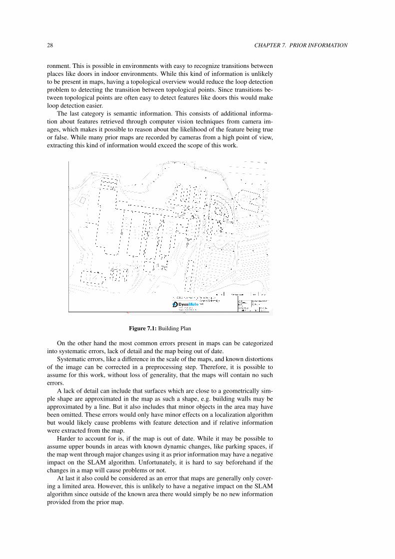
Figure 7.1: Building Plan

On the other hand the most common errors present in maps can be categorizedinto systematic errors, lack of detail and the map being out of date.

Systematic errors, like a difference in the scale of the maps, and known distortionsof the image can be corrected in a preprocessing step. Therefore, it is possible toassume for this work, without loss of generality, that the maps will contain no sucherrors.

A lack of detail can include that surfaces which are close to a geometrically sim-ple shape are approximated in the map as such a shape, e.g. building walls may beapproximated by a line. But it also includes that minor objects in the area may havebeen omitted. These errors would only have minor effects on a localization algorithmbut would likely cause problems with feature detection and if relative informationwere extracted from the map.

Harder to account for is, if the map is out of date. While it may be possible toassume upper bounds in areas with known dynamic changes, like parking spaces, ifthe map went through major changes using it as prior information may have a negativeimpact on the SLAM algorithm. Unfortunately, it is hard to say beforehand if thechanges in a map will cause problems or not.

At last it also could be considered as an error that maps are generally only cover-ing a limited area. However, this is unlikely to have a negative impact on the SLAMalgorithm since outside of the known area there would simply be no new informationprovided from the prior map.

29

Taking a look at the literature on using prior maps the most common types of mapsare hand-drawn maps, satellite or aerial images and blueprint-like maps.

The focus, when hand-drawn maps are used, is typically not to improve the SLAMalgorithm but rather to find a middle ground between the hand-drawn map and the mapthe robot is building with the goal of later using additional information like directionspresent on the hand-drawn map [26][27]. Recognizing such information is useful forrobots that have to interact with humans, but can be considered uninteresting for heavyproduction vehicles, which are the target of this work.

Satellite or aerial images will most likely lack fine details and include details andinformation which can not be seen by the robot, but will be accurate aside from this.However, the information in these maps is not directly accessible. Rather, it is neces-sary to extract the required information using image processing techniques. Depend-ing on how accurate this extraction works even more details will be lost and the resultcan be considered similar to a blueprint-like map. However, since image processingtechniques may also detect false or miss relevant details this extraction is often doneby hand for research purposes [12].

Blueprint-like maps will typically lack a lot of details of the real area but willstill provide strong boundaries for a localization algorithm. The most likely featuresthat could be extracted from such a map would be corners and lines, but the scans ofthe robot would detect more corners and less constant lines because of the additionaldetails it can recognize. While detecting such features would be possible, matching adetected feature to the correct feature on the prior map would be prone to errors. Tominimize the effect of such errors it would be necessary to use switchable constraintsin the Graph-SLAM algorithm.

Figure 7.2: Robot scans of the area

Figure 7.1 shows a building plan we will be using in this work. Aside from thebuildings we can see additional information in a gray font. Mainly the building num-bers and the outlines of the streets and other borders that are easy to recognize forhumans like fences. Since many of these structures will not be visible on a range scanthe information displayed in gray can be filtered out. It can also be seen that the scaleof the map is 1:1500. Since the map was meant to be printed as an A3 document, thisinformation allows us to convert the map to a correct scaled grid map. The buildingoutlines contain, as expected from such a plan, very little details. A typical range scan

30 CHAPTER 7. PRIOR INFORMATION

will pick up other details of the buildings, e.g. entries and railings, not contained inthis map.

Figure 7.3: Building Plan and scans overlayed

Figure 7.4: Closer view of the overlayed area

In more detail, in Figure 7.2 we can see the scans of the agent we use in this paperwith accurate pose estimates from a RTK GPS. Without additional information it ishard to tell which part of the map was explored. But with an accurate guess for the

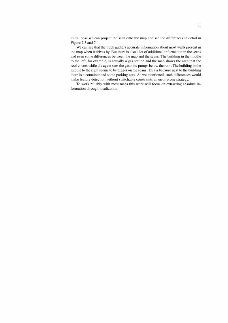
31

initial pose we can project the scan onto the map and see the differences in detail inFigure 7.3 and 7.4.

We can see that the truck gathers accurate information about most walls present inthe map when it drives by. But there is also a lot of additional information in the scansand even some differences between the map and the scans. The building in the middleto the left, for example, is actually a gas station and the map shows the area that theroof covers while the agent sees the gasoline pumps below the roof. The building in themiddle to the right seems to be bigger on the scans. This is because next to the buildingthere is a container and some parking cars. As we mentioned, such differences wouldmake feature detection without switchable constraints an error prone strategy.

To work reliably with most maps this work will focus on extracting absolute in-formation through localization.

Chapter 8

Localization

To extract absolute information from the prior map through localization there are mul-tiple approaches we could use. Two common algorithms to the localization problemare the extended Kalman filter (EKF) and the Monte Carlo Localization (MCL). How-ever, since we want to localize on an inaccurate map, our requirements to a localizationalgorithm are slightly different. Since the prior map may contain blank areas, wherethe uncertainty of the localization algorithm could quickly increase, a localizationalgorithm that supports multi-hypothesis upon reentering known areas is preferable.Since the EKF does not support multi-hypothesis and other papers already used MCLsuccessfully on prior maps [12] we decided to use MCL in this paper as well. WhileVysotska and Stachniss used ICP registration successfully for the localization prob-lem on a prior map it is unclear how well this behaves on incomplete maps wheremultiple hypotheses might be necessary.

The idea behind MCL is quite simple. Instead of representing the pose of therobot as a probability function it is represented by multiple particles which containpose information where the robot could be. If the robot moves, the particles each drawa sample from the motion model of the robot and use this noisy motion instead ofdirectly using the odometry information. Since every particle draws a different samplethe particles then spread out. This step is known as the motion update.

The other step of MCL is the sensor update. This step is triggered, if we have arange scan of the robot at the current pose, and calculates the probability of each par-ticle perceiving the current range scan from its current pose. With these probabilitiesthe unlikely poses are then thinned out and new copies of the likely poses are created.This step is commonly known as resampling. However, unlike with the motion up-date there are multiple approaches to the calculation of the probabilities as well as theresampling.

The most accurate algorithm for the probability calculation of the sensor updateis to trace the rays of each detection from the sensor to the detected point. This waydetections of objects with other obstacles in the path of the ray can also be consid-ered to be unlikely. However, this process is rather slow and prior maps will rarelyhave enough details in front of walls to really make use of this feature. It also has aunsmooth probability distribution over the map and would lead to large errors if anobject present in the map would not appear on the sensor readings. A considerablyfaster solution was presented by Thrun et al. [21], which only uses the detected pointswithout tracing the path to the detection. Since in this case the pose of the sensors isonly relevant to transform the sensor readings, it is possible to calculate a lookup tablein the size of the map that contains the likelihood of a detection being seen at a certainpoint in the map. While calculating such a likelihood field may be slow, depending onthe map, it only needs to be calculated once and can then be used as long as the mapis not changed.

33

34 CHAPTER 8. LOCALIZATION

Each cell in the lookup table can be computed as a function of the distance fromthe cell ci j to the closest occupied cell oi j on the map m

p(ci j|m) = zrandom + zhit ∗1√

2πσ2hit

exp(−

ci joi j2

2σ2hit

), (8.1)

where zrandom, zhit and σhit are tuneable parameters. zrandom is used for a uniformdistribution across the map to simulate sensor errors, dynamic objects and errors ofthe prior map. zhit and σhit on the other hand represent a normal distribution aroundoccupied cells in the map. σhit can be not only be used to simulate the accuracy of thesensors but also to simulate inaccuracies of the prior map.

The probability of a scan is then

p(zt |xt ,m) =N

∏i=1

p(zit |xt ,m) =

N

∏i=1

p(ckl |m) (8.2)

with ckl being the cell the detection zit falls into if the pose of the robot is xt . With this

formula we can define the weight wq of the particle q at the time t as

wq = p(zt |xqt ,m). (8.3)

To avoid unnecessary resampling operations we first calculate the effective samplesize (ESS) [28]

ESS =N

1+ cv2 (8.4)

where cv2 denotes the variation of the weights of the particles

cv2 =var(w)µ(w)

=1N

N

∑i=1

(N ·wi−1)2 (8.5)

with var(w) being the variance of the weights and µ(w) being the mean of the weights.If the ESS drops below a percentage of the sample size

ESS < BETA ·N (8.6)

the particle pool contains too many unlikely samples and resampling is necessary.During resampling the particle weights are normalized, so that all weights sum

up to 1. Then the numerical range between 0 and 1 is mapped towards the particlesin a way that each particle occupies a length according to its weight. After that Nnumbers between 0 and 1 are generated and for each number a copy of the particle,this function maps to, is generated. While it is possible to simply use N random values,a more reliable behaviour can be achieved by generating only a single random valuebetween 0 and 1/N and placing the other N− 1 numbers at 1/N intervals after thisrandom number. This strategy is also known as low variance resampling.

In this work we will be the low variance resampling strategy, with logarithmicweights instead of the weights directly, together with the likelihood fields accordingto Thrun et al. We are using logarithmic weights to decrease the influence of singleoutliers, which is especially important due to the high noise of the sensors. Low vari-ance resampling is used since it is the most robust strategy to keep a diverse particlepool alive.

Chapter 9

Results

9.1 Test setup

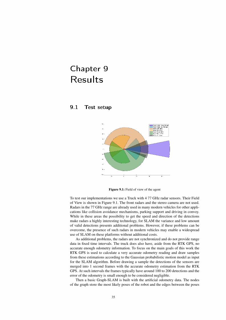
Figure 9.1: Field of view of the agent

To test our implementations we use a Truck with 4 77 GHz radar sensors. Their Fieldof View is shown in Figure 9.1. The front radars and the stereo camera are not used.Radars in the 77 GHz range are already used in many modern vehicles for other appli-cations like collision avoidance mechanisms, parking support and driving in convoy.While in these areas the possibility to get the speed and direction of the detectionsmake radars a highly interesting technology, for SLAM the variance and low amountof valid detections presents additional problems. However, if these problems can beovercome, the presence of such radars in modern vehicles may enable a widespreaduse of SLAM on these platforms without additional costs.

As additional problems, the radars are not synchronized and do not provide rangedata in fixed time intervals. The truck does also have, aside from the RTK GPS, noaccurate enough odometry information. To focus on the main goals of this work theRTK GPS is used to calculate a very accurate odometry reading and draw samplesfrom these estimations according to the Gaussian probabilistic motion model as inputfor the SLAM algorithm. Before drawing a sample the detections of the sensors aremerged into 1 second frames with the accurate odometry estimation from the RTKGPS. At such intervals the frames typically have around 100 to 200 detections and theerror of the odometry is small enough to be considered negligible.

Then a basic Graph-SLAM is built with the artificial odometry data. The nodesof the graph store the most likely poses of the robot and the edges between the poses

35

36 CHAPTER 9. RESULTS

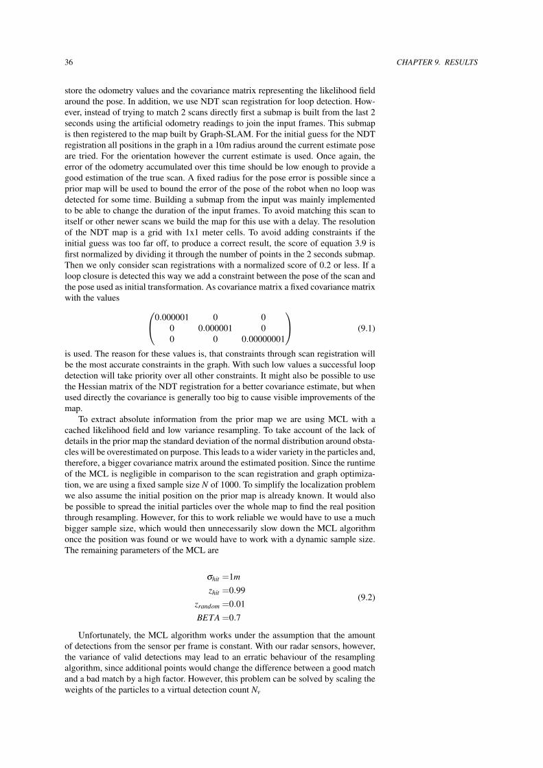
store the odometry values and the covariance matrix representing the likelihood fieldaround the pose. In addition, we use NDT scan registration for loop detection. How-ever, instead of trying to match 2 scans directly first a submap is built from the last 2seconds using the artificial odometry readings to join the input frames. This submapis then registered to the map built by Graph-SLAM. For the initial guess for the NDTregistration all positions in the graph in a 10m radius around the current estimate poseare tried. For the orientation however the current estimate is used. Once again, theerror of the odometry accumulated over this time should be low enough to provide agood estimation of the true scan. A fixed radius for the pose error is possible since aprior map will be used to bound the error of the pose of the robot when no loop wasdetected for some time. Building a submap from the input was mainly implementedto be able to change the duration of the input frames. To avoid matching this scan toitself or other newer scans we build the map for this use with a delay. The resolutionof the NDT map is a grid with 1x1 meter cells. To avoid adding constraints if theinitial guess was too far off, to produce a correct result, the score of equation 3.9 isfirst normalized by dividing it through the number of points in the 2 seconds submap.Then we only consider scan registrations with a normalized score of 0.2 or less. If aloop closure is detected this way we add a constraint between the pose of the scan andthe pose used as initial transformation. As covariance matrix a fixed covariance matrixwith the values 0.000001 0 0

0 0.000001 00 0 0.00000001

(9.1)

is used. The reason for these values is, that constraints through scan registration willbe the most accurate constraints in the graph. With such low values a successful loopdetection will take priority over all other constraints. It might also be possible to usethe Hessian matrix of the NDT registration for a better covariance estimate, but whenused directly the covariance is generally too big to cause visible improvements of themap.

To extract absolute information from the prior map we are using MCL with acached likelihood field and low variance resampling. To take account of the lack ofdetails in the prior map the standard deviation of the normal distribution around obsta-cles will be overestimated on purpose. This leads to a wider variety in the particles and,therefore, a bigger covariance matrix around the estimated position. Since the runtimeof the MCL is negligible in comparison to the scan registration and graph optimiza-tion, we are using a fixed sample size N of 1000. To simplify the localization problemwe also assume the initial position on the prior map is already known. It would alsobe possible to spread the initial particles over the whole map to find the real positionthrough resampling. However, for this to work reliable we would have to use a muchbigger sample size, which would then unnecessarily slow down the MCL algorithmonce the position was found or we would have to work with a dynamic sample size.The remaining parameters of the MCL are

σhit =1m

zhit =0.99zrandom =0.01BETA =0.7

(9.2)

Unfortunately, the MCL algorithm works under the assumption that the amountof detections from the sensor per frame is constant. With our radar sensors, however,the variance of valid detections may lead to an erratic behaviour of the resamplingalgorithm, since additional points would change the difference between a good matchand a bad match by a high factor. However, this problem can be solved by scaling theweights of the particles to a virtual detection count Nv

9.2. SIMULATION RESULTS 37

w′q = (wq)

NvN (9.3)

where N represents the actual amount of detections.Since the localization worked without this change, the MCL algorithm was left

unchanged in this work.

9.2 Simulation results

We already included a map of the test data without adding additional noise in Figure7.2 and a picture of the prior map, which we will use with the MCL algorithm, canbe seen in Figure 7.1. The area was explored starting at the bottom entry of the mapdriving around the building in the middle to the right in anticlockwise direction thengoing up to the area in the top left and then turning and going back towards the begin-ning, passing the building in the middle to the right on the left side. The test data is 4minutes long. To test the scan registration we added noise according to the GaussianMotion Model with the parameters

α1 =0.01 meters/meter

α2 =0.005 meters/degree

α3 =0.25 degrees/meter

α4 =0.025 degrees/degree

σminxy =0.04 meters

σminφ =0.2 degrees

(9.4)

Figure 9.2: Test data for scan registration

A map built with the noisy odometry data can be seen in Figure 9.2. While thetop of the map looks quite clean and does not show any obvious errors it is easy torecognize a rotational error in the building in the middle to the right. In this area thereare also less obvious features affected by this rotational error around the building,which increases the chance of a successful scan registration and its accuracy.

38 CHAPTER 9. RESULTS

Figure 9.3: Result of using scan registration

In Figure 9.3 we can see the result of applying scan registration to the noisy inputdata. We can see that the building in the middle now shows no signs of being recordedtwice. There is still some visible error on the wall at the slope in the bottom right, butthe improvement compared to the noisy data is still huge.

Figure 9.4: scan registration results projected onto the building plan

However, since no pairwise scan registration is performed, only errors that accu-mulate inside a loop can be minimized and the resulting map will only be plausibleinside such loops. If the robot moves in a pattern that has no loops the error of the mapcan quickly increase and lead to a state where even scan registration would not workwith a local search approach. However, even in our example the corrected map is a lotless accurate than it looks like. This can be seen if we project it onto the building planof the area we already presented in Figure 7.1. In Figure 9.4 we can see that the resultof the scan registration does not fit the building plan. This is caused by an error in the

9.2. SIMULATION RESULTS 39

rotation before the beginning of the loop detected through scan registration. This errorcan not be corrected by scan registration.

To allow the use of local scan registration algorithms and improve the overall qual-ity of the resulting map we decided to extract information from a prior map. Due tothe test data being characterized by an initial seed for the random number generatorand the SLAM algorithm running at the same time as the creation of the test data, theuse of MCL changed the input map, since the sampling of MCL will change the inter-nal random seed and lead to different sampling for the artificial odometry. However,since the positive effects of using a prior map on the overall quality can also be seenon different input data and works stable independent of the random seed, we decidedto also change the motion model parameters and show the effect on another input. Themotion model parameters used for the algorithm with MCL are

α1 =0.01 meters/meter

α2 =0.005 meters/degree

α3 =0.5 degrees/meter

α4 =0.05 degrees/degree

σminxy =0.04 meters

σminφ =0.2 degrees

(9.5)

Since the MCL will bound the error of the pose it is possible to work with a lessaccurate odometry.

Figure 9.5: Raw test data with changed error values and seed used for MCL in the followingFigures

The test data created with these inputs can be seen in Figure 9.5. While in thiscase the open area in the top left seems to be more accurate due to the rotational errorsnegating themselves, the building in the middle to the right is hardly recognizableanymore. However, if MCL is run on the prior map and these new constraints areadded the map shows a drastic improvement, which can be seen in Figure 9.6.

Even though in a lot of places the contours of the obstacles seem a bit blurred, themap fits the prior information and all obstacles are clearly recognizable. The only areawhere an obvious error can be seen is the wall of the slope in the bottom right again.This can be explained by the lack of information on the prior map in that area and theinaccuracy of the building in the middle to the right. These effects can lead to a largercovariance matrix of the MCL constraints, which means that the errors of the noisyodometry data are less likely to be corrected.

40 CHAPTER 9. RESULTS

Figure 9.6: Test data from Figure 9.5 with added constraints from running MCL on the priormap but without loop detection

Figure 9.7: Test data from Figure 9.5 with added constraints from MCL and loop detection

Finally, we also run scan registration together with MCL on the noisy data, sincescan registration does not change the random seed. The result can be seen in Figure9.7. It can be seen that the resulting map shows sharper contours of the objects andstill fits the prior map very accurately. The error at the wall in the bottom right wasalso corrected by the scan registration. However, if we compare it to the result of usingscan registration alone we can see that the contours in the top left are less sharp. Thisis mostly due to the increased noise parameters in the motion model, but also due tothe fact that the obstacles of the prior map in this area contain almost no details.

Since the development of the algorithm presented here was on a virtual machinerunning Linux and the focus was on creating a working algorithm rather than onlinecapability the result is rather slow. On a Intel i5-2500 (3,3 GHz) with Windows 7 anda virtual machine with Ubuntu the final run with MCL and scan registration took 25minutes to process, while the input was only 4 minutes long.

Chapter 10

Conclusions

In this work we presented a complete Graph-SLAM algorithm, which extracts poseestimates from a rough map and adds them as additional constraints. In comparison toother papers we only used radar sensors which are legal to use in public street traffic.

We showed that Graph-SLAM works well with radar sensors, even though thereis no fixed amount of detections, and that prior information in form of absolute posesfrom a localization algorithm can significantly improve the result of Graph-SLAM andeasily be combined with scan registration. We also showed that NDT scan registration,even though it was developed as a way to handle dense point clouds, works well onsparse data as well in the context of Graph-SLAM.

While we would have liked to present results with real odometry values we areconfident that the simulation results show that the algorithm could be used on a robotwith odometry readings instead of an GPS sensor.

However, in the field of robotics it is important to weight the use of the algorithmoff against the negative impact it may have on society. While our algorithm does notactually perform any actions and only gathers information, this information is mainlyof interest so that the robot can later on perform informed actions.

Since GPS sensors are already present in most areas on earth and provide a sim-pler solution to the SLAM problem our algorithm is most likely to be used in spaceprograms, indoor areas, underground areas and other areas that have not enough satel-lite coverage to calculate a proper GPS position. We can assume that an applicationin underground areas or in a space program will prevent humans from having to workin these, in most cases, hazardous areas. These are, obviously, desired applications.While the use in indoor environments and areas without enough satellite coveragemay as well be of use in the case of catastrophes, here our algorithm may lead torobots replacing humans in perfectly safe working places. However, we can assumethat, with some additional effort, a map may be built in these safe areas anyways andas such our work does not have a strong influence on this topic. We do not expect ouralgorithm to be of use for any military operations, since the military will in most caseshave sufficient satellite coverage in outdoor areas and in indoor and underground areasreal time information will be much more valuable since an undisturbed exploration runthrough a building is very unlikely. We also assume that military operations on extraterrestrial bodies will not take place any time soon and leave the discussion about it toanother generation.

For future works we propose to validate the results of the simulations of this workwith real odometry data and to optimize the code to run in real time even on largermaps. For example the 10m radius for the scan registration is quite time consumingand it is probably not necessary to add MCL constraints for every pose since theerror that will accumulate between two poses is rather low. In addition, closed loopsin areas the agent is not currently exploring could be temporarily removed from the

41

42 CHAPTER 10. CONCLUSIONS

graph to only optimize the entry and exit points of the loop with EKF estimations forthe constraints between these nodes.

Bibliography

[1] M. Montemerlo, S. Thrun, D. Koller, and B. Wegbreit. FastSLAM 2.0: An im-proved particle filtering algorithm for simultaneous localization and mappingthat provably converges. In Proceedings of the Sixteenth International JointConference on Artificial Intelligence (IJCAI), Acapulco, Mexico, 2003. IJCAI.

[2] J.J. Leonard and H.F. Durrant-Whyte. Mobile robot localization by trackinggeometric beacons. Robotics and Automation, IEEE Transactions on, 7(3):376–382, Jun 1991.

[3] Sebastian Thrun, Yufeng Liu, Daphne Koller, Andrew Y Ng, Zoubin Ghahra-mani, and Hugh Durrant-Whyte. Simultaneous localization and mapping withsparse extended information filters. The International Journal of Robotics Re-search, 23(7-8):693–716, 2004.

[4] Tim Bailey, Juan Nieto, Jose Guivant, Michael Stevens, and Eduardo Nebot.Consistency of the EKF-SLAM algorithm. In Intelligent Robots and Systems,2006 IEEE/RSJ International Conference on, pages 3562–3568. IEEE, 2006.

[5] Feng Lu and Evangelos Milios. Globally consistent range scan alignment forenvironment mapping. Autonomous robots, 4(4):333–349, 1997.

[6] Rainer Kümmerle, Giorgio Grisetti, Hauke Strasdat, Kurt Konolige, and Wol-fram Burgard. g 2 o: A general framework for graph optimization. In Roboticsand Automation (ICRA), 2011 IEEE International Conference on, pages 3607–3613. IEEE, 2011.

[7] Paul J Besl and Neil D McKay. Method for registration of 3-D shapes. InRobotics-DL tentative, pages 586–606. International Society for Optics and Pho-tonics, 1992.

[8] Peter Biber and Wolfgang Straßer. The normal distributions transform: A newapproach to laser scan matching. In Intelligent Robots and Systems, 2003.(IROS2003). Proceedings. 2003 IEEE/RSJ International Conference on, volume 3,pages 2743–2748. IEEE, 2003.

[9] Todor Stoyanov, Martin Magnusson, and Achim J. Lilienthal. Fast and accuratescan registration through minimization of the distance between compact 3d ndtrepresentations. The International Journal of Robotics Research, 31:1377–1393,2012.

[10] Edwin B Olson. Real-time correlative scan matching. In Robotics and Au-tomation, 2009. ICRA’09. IEEE International Conference on, pages 4387–4393.IEEE, 2009.

43

44 BIBLIOGRAPHY

[11] Radu Bogdan Rusu, Nico Blodow, and Michael Beetz. Fast point featurehistograms (FPFH) for 3D registration. In Robotics and Automation, 2009.ICRA’09. IEEE International Conference on, pages 3212–3217. IEEE, 2009.

[12] Rainer Kümmerle, Bastian Steder, Christian Dornhege, Alexander Kleiner, Gior-gio Grisetti, and Wolfram Burgard. Large scale graph-based SLAM using aerialimages as prior information. Autonomous Robots, 30(1):25–39, 2011.

[13] Olga Vysotska and Cyrill Stachniss. Exploiting building information from pub-licly available maps in graph-based slam. In Intelligent Robots and Systems(IROS), 2016 IEEE/RSJ International Conference on, pages 4511–4516. IEEE,2016.

[14] Martin P Parsley and Simon J Julier. Exploiting prior information in Graph-SLAM. In Robotics and Automation (ICRA), 2011 IEEE International Confer-ence on, pages 2638–2643. IEEE, 2011.

[15] Paul Newman, John Leonard, JD Tardó, and José Neira. Explore and re-turn: Experimental validation of real-time concurrent mapping and localization.In Robotics and Automation, 2002. Proceedings. ICRA’02. IEEE InternationalConference on, volume 2, pages 1802–1809. IEEE, 2002.

[16] Martin P Parsley and Simon J Julier. Towards the exploitation of prior infor-mation in SLAM. In Intelligent Robots and Systems (IROS), 2010 IEEE/RSJInternational Conference on, pages 2991–2996. IEEE, 2010.

[17] Martin Magnusson. The three-dimensional normal-distributions transform: anefficient representation for registration, surface analysis, and loop detection.2009.

[18] Niko Sünderhauf and Peter Protzel. Switchable constraints for robust pose graphslam. In Intelligent Robots and Systems (IROS), 2012 IEEE/RSJ InternationalConference on, pages 1879–1884. IEEE, 2012.

[19] Pratik Agarwal, Gian Diego Tipaldi, Luciano Spinello, Cyrill Stachniss, andWolfram Burgard. Robust map optimization using dynamic covariance scaling.In Robotics and Automation (ICRA), 2013 IEEE International Conference on,pages 62–69. IEEE, 2013.

[20] Probabilistic motion models - MRPT. http://www.mrpt.org/tutorials/

programming/odometry-and-motion-models/probabilistic_motion_

models/. Accessed: 2016-11-24.

[21] Sebastian Thrun, Wolfram Burgard, and Dieter Fox. Probabilistic robotics. MITpress, 2005.

[22] Timothy A Davis. Direct methods for sparse linear systems. SIAM, 2006.

[23] Yanqing Chen, Timothy A Davis, William W Hager, and Sivasankaran Raja-manickam. Algorithm 887: Cholmod, supernodal sparse cholesky factorizationand update/downdate. ACM Transactions on Mathematical Software (TOMS),35(3):22, 2008.

[24] D.M. Rosen, L. Carlone, A.S. Bandeira, and J.J. Leonard. A certifiably correctalgorithm for synchronization over the special Euclidean group. In Intl. Work-shop on the Algorithmic Foundations of Robotics (WAFR), San Francisco, CA,December 2016.

[25] Martin Peter Parsley. Simultaneous localisation and mapping with prior infor-mation. PhD thesis, UCL (University College London), 2011.

BIBLIOGRAPHY 45

[26] Keisuke Matsuo and Jun Miura. Outdoor visual localization with a hand-drawnline drawing map using fastslam with pso-based mapping. In Intelligent Robotsand Systems (IROS), 2012 IEEE/RSJ International Conference on, pages 202–207. IEEE, 2012.

[27] Federico Boniardi, Bahram Behzadian, Wolfram Burgard, and Gian DiegoTipaldi. Robot navigation in hand-drawn sketched maps. In Mobile Robots(ECMR), 2015 European Conference on, pages 1–6. IEEE, 2015.

[28] Jun S Liu, Rong Chen, and Tanya Logvinenko. A theoretical framework forsequential importance sampling with resampling. In Sequential Monte Carlomethods in practice, pages 225–246. Springer, 2001.