integrating and updating of sapwat and planwat …programme, the fao published the irrigation and...
TRANSCRIPT

INTEGRATING AND UPDATING OF SAPWAT AND PLANWAT TO CREATE A POWERFUL AND
USER-FRIENDLY IRRIGATION PLANNING TOOL Program version 1.0
Report to the
WATER RESEARCH COMMISSION
by
P S van Heerden, C T Crosby, B Grové, N Benadé E Theron, R E Schulze & M H Tewolde
WRC REPORT NO. TT 391/08
MARCH 2009
2
Obtainable from: Water Research Commission Private Bag X03 Gezina 0031 The publication of this report emanates from a project entitled: Integrating and Upgrading of SAPWAT and PLANWAT to create a powerful and user-friendly irrigation planning tool (WRC Project No. K5/1578//4).
ISBN 978-1-77005-828-6 Printed in the Republic of South Africa
DISCLAIMER
The report has been reviewed by the Water Research Commission (WRC) and approved for publication. Approval does not signify that the contents necessarily reflect the views and policies of the WRC, nor does mention of trade names or commercial products constitute endorsement or recommendation for use.

3
Acknowledgements
The Water Research Commission: The SAPWAT program, which was developed and tested with WRC funding, is now generally in use and is also the accepted model for use in the calculation of irrigation requirements for registration and licensing purposes by the Department of Water Affairs and Forestry. The model has been developed through two consecutive WRC research projects. This was followed by two technology transfer projects to demonstrate the application of SAPWAT on seven irrigation schemes. The application of SAPWAT has highlighted the importance of continuous upgrading and further development. The research team want to acknowledge the support, funding and management of these projects by the WRC over the past 15 years, which led to the upgrading and revision of SAPWAT and finally resulted in the current program, SAPWAT3. Appreciation is expressed to the WRC research managers Dr G.C. Green, Mr D.S. van der Merwe, Dr G.R. Backeberg and Dr A.J. Sanewe who provided guidance in this process.
Members of the Reference Group for advice and support:
Dr. A.J. Sanewe Water Research Commission (Chairman) Dr. G.R. Backebereg Water Research Commission Prof. J.G. Annandale University of Pretoria Prof. A.T.P. Bennie University of the Free State Mr. C. Chunda DWAF Mr. W.L. de Lange CSIR Stellenbosch Mr. D. Haarhoff GWK Ltd Prof. G.P.W. Jewitt University of KwaZulu-Natal Dr. P. Myburgh ARC Infruitec Nietvoorbij Mr. F.P.J. van der Merwe DWAF
Members of the project team for cooperation, advice and support. Members of the Irrigation Efficiency project (WRC Project K5/1482/4) team for discussions and advice on the inclusion of water distribution and irrigation system efficiencies (Mr. F.B. Reinders, Mr. F.H. Koegelenberg, Ms. I. van der Stoep and Dr. N. LeCler). Prof. D.J. de Waal, Department of Mathematical Statistics, University of the Free State, for advice on statistical approaches. Prof. S. Walker, Department of Soil, Crop and Climate Sciences, University of the Free State, for patient listening, explaining and advising on matters pertaining agro-meteorology. Dr. C.H. Barker, GIS Laboratory, Department of Geography – University of the Free State, for preparing and extracting the maps used in SAPWAT3 weather data module. Mr. G.C. de Kock, retired agronomist of the Department of Agriculture, Karoo Region, for advice and assistance regarding crop data of drought resistant and specialised crops grown in semi-arid and arid areas.

4
Mr. W. Bruwer, CEO of Orange-Vaal Water Users Association, as a tester and for advice on user requirements and user-friendliness. Members of the dBase dBVIP group for problem solving and advice on programming (Robert Bravery, Greg Hill, Jan Hoeltering, Ivar B. Jessen, Todd Kreuter, Jonny Kwekkeboom, Gerald Lightsey, Eric Logan, Jean-Pierre Martel, Ken Mayer, Ronnie McGregor, Michael Nuwer, Rob Rickard, Geoff Wass and Roland Wingerter). All the agricultural scientists, technicians, water user association personnel and farmers who willingly shared their knowledge of and experience in crop irrigation requirements and crop characteristics.

5
Table of Contents
EXECUTIVE SUMMARY ............................................................................................ 9
CHAPTER 1 INTRODUCTION ................................................................................. 13
1.1 BACKGROUND TO THE DEVELOPMENT OF SAPWAT3 ............................................... 13 1.2 OBJECTIVES FOR DEVELOPING SAPWAT3 ............................................................... 16 1.3 POTENTIAL APPLICATION OF SAPWAT3 .................................................................. 17
CHAPTER 2 USING SAPWAT3 ................................................................................ 19
2.1 INSTALLING ............................................................................................................... 19 2.1.1 Single user installation ......................................................................................... 19 2.1.2 Multi-user installation .......................................................................................... 19 2.1.3 System requirements ............................................................................................. 20 2.1.4 Data security and reinstallation ........................................................................... 20 2.2 INTRODUCTION TO THE PROGRAM ............................................................................. 20 2.3 THE MAIN PROGRAM ................................................................................................. 23 2.4 THE MENU ITEMS ....................................................................................................... 36 2.4.1 Estimate irrigation requirements .......................................................................... 37 2.4.2 Irrigation systems (refer to Chapter 10) ............................................................... 37 2.4.3 Distribution systems and efficiencies (refer to Chapter 10) ................................. 37 2.4.4 Soil (refer to Chapter 5) ........................................................................................ 38 2.4.5 Weather stations (refer to Chapter 4) ................................................................... 39 2.4.6 Climate (refer to Chapter 3) ................................................................................. 41 2.4.7 Crop data (refer to Chapter 6) ............................................................................. 43 2.4.8 Crop groups .......................................................................................................... 44 2.4.9 Countries (refer to Chapter 13) ............................................................................ 44 2.4.10 Address list .......................................................................................................... 45
CHAPTER 3 CLIMATE .............................................................................................. 46
3.1 INTRODUCTION ......................................................................................................... 46 3.2 APPLICATION IN SAPWAT3 ..................................................................................... 49 3.2.1 Data organisation ................................................................................................. 50
CHAPTER 4 WEATHER STATIONS ....................................................................... 51
4.1 INTRODUCTION ......................................................................................................... 51 4.2 APPLICATION IN SAPWAT3 ..................................................................................... 51 4.2.1 Importing weather station data ............................................................................. 51
CHAPTER 5 SOIL ....................................................................................................... 55
5.1 INTRODUCTION ......................................................................................................... 55 5.2 SOIL IN IRRIGATION .................................................................................................. 55 5.3 SOIL WATER .............................................................................................................. 55 5.4 EVAPORATION FROM THE SOIL SURFACE ................................................................... 57 5.5 APPLICATION IN SAPWAT3 ..................................................................................... 59
CHAPTER 6 CROPS ................................................................................................... 60
6.1 INTRODUCTION ......................................................................................................... 60 6.2 THE FOUR-STAGE CROP CYCLE .................................................................................. 60

6
6.3 APPLICATION IN SAPWAT3 ..................................................................................... 63 6.3.1 Data organisation ................................................................................................. 63 6.4 METHODOLOGY ........................................................................................................ 64 6.4.1 Possible improvements ......................................................................................... 66
CHAPTER 7 EVAPOTRANSPIRATION ................................................................. 67
7.1 FACTORS AFFECTING EVAPOTRANSPIRATION ............................................................ 67 7.2 EVAPOTRANSPIRATION CONCEPTS ............................................................................ 68 7.2.1 Reference crop evapotranspiration ...................................................................... 69 7.2.2 Crop evapotranspiration under standard conditions (ETc) .................................. 70 7.2.3 Crop evapotranspiration under non-standard conditions (ETc adj) ...................... 70 7.3 CALCULATING REFERENCE EVAPOTRANSPIRATION ................................................... 71 7.3.1 Introduction .......................................................................................................... 71 7.3.2 Calculating reference evapotranspiration values ................................................. 71 7.4 FITTING A REGRESSION TO CALCULATED ET0 VALUES .............................................. 74 7.5 APPLICATION IN SAPWAT3 ..................................................................................... 80 7.5.1 The SAPWAT3 ET0 calculator .............................................................................. 80
CHAPTER 8 ETC - DUAL CROP COEFFICIENT (KC = KCB + KE) ..................... 81
8.1 TRANSPIRATION COMPONENT ................................................................................... 81 8.1.1 Upper limit of Kc max .............................................................................................. 81 8.1.2 Exposed and wetted soil fraction (few) .................................................................. 81 8.1.3 Fraction of soil surface wetted by irrigation or precipitation .............................. 83 8.2 DAILY CALCULATION OF KE ...................................................................................... 84 8.3 APPLICATION IN SAPWAT3 ..................................................................................... 85
CHAPTER 9 ETC UNDER SOIL WATER STRESS CONDITIONS ..................... 86
9.1 SOIL WATER AVAILABILITY ....................................................................................... 86 9.1.1 Total available water (TAW) ................................................................................ 86 9.1.2 Readily available water (RAW) ............................................................................ 86 9.2 WATER STRESS COEFFICIENT (KS) ............................................................................. 87 9.3 SOIL WATER BALANCE .............................................................................................. 88 9.3.1 Limits on Dr,i ......................................................................................................... 89 9.3.2 Initial depletion ..................................................................................................... 90 9.3.3 Precipitation (P), runoff (RO) and irrigation (I) .................................................. 90 9.3.4 Capillary rise (CR) ............................................................................................... 90 9.3.5 Evapotranspiration ............................................................................................... 90 9.3.6 Deep percolation ................................................................................................... 90 9.4 FORECASTING OR ALLOCATING IRRIGATIONS ............................................................ 91 9.5 EFFECTS OF SOIL SALINITY ........................................................................................ 91 9.6 YIELD-SALINITY RELATIONSHIP ................................................................................ 92 9.7 YIELD-MOISTURE STRESS RELATIONSHIP .................................................................. 93 9.7.1 Limitations ............................................................................................................ 94 9.7.2 Application ............................................................................................................ 94
CHAPTER 10 IRRIGATION SYSTEMS .................................................................. 96
10.1 THE IRRIGATION SYSTEM DATA TABLE .................................................................... 96 10.1.1 On-farm water distribution ................................................................................. 97

7
CHAPTER 11 ENTERPRISE BUDGETS ................................................................. 99
11.1 INTRODUCTION ....................................................................................................... 99 11.2 DEVELOPMENT OF SPREAD SHEET MODEL TO DEMONSTRATE THE
INCORPORATION OF GROSS MARGIN CALCULATIONS IN SAPWAT3 .................... 100 11.3 CALCULATION OF CROP YIELD .............................................................................. 106 11.4 APPLICATION IN SAPWAT3 ................................................................................. 107 11.4.1 Data organisation ............................................................................................. 109
CHAPTER 12 WATER HARVESTING .................................................................. 110
12.1 THEORETICAL OVERVIEW ...................................................................................... 110 12.1.1 Introduction ...................................................................................................... 110 12.1.2 Domestic rainwater harvesting technology ...................................................... 111 12.1.3 Catchment surface ............................................................................................ 111 12.1.4 Gutters .............................................................................................................. 113 12.1.5 Down pipes ....................................................................................................... 114 12.1.6 Water quality maintaining measures ................................................................ 114 12.1.7 Storage facilities ............................................................................................... 115 12.1.8 Low cost pumps ................................................................................................. 118 12.1.9 Aquaculture ....................................................................................................... 120 12.1.10 Grey water ...................................................................................................... 121 12.1.11 Irrigation requirement for vegetable crops .................................................... 121 12.1.12 Application of DRWH in SAPWAT3 ............................................................... 122
CHAPTER 13 COUNTRIES ..................................................................................... 123
CHAPTER 14 APPLYING SAPWAT3 .................................................................... 124
14.1 ANALYSING IRRIGATION STRATEGIES.................................................................... 124 14.1.1 The Dundee example ......................................................................................... 124 14.1.2 The Douglas example ........................................................................................ 128
REFERENCES .......................................................................................................... 135

8

9
EXECUTIVE SUMMARY
SAPWAT3 is essentially an enhanced and improved version of SAPWAT, the program that is extensively applied in South Africa and developed to establish a decision-making procedure for the estimation of crop irrigation requirements by irrigation engineers, planners and agriculturalists. Subsequent to the development of the current SAPWAT programme, the FAO published the Irrigation and Drainage report No. 56, Crop evapotranspiration. Guidelines for computing crop water requirements. This intuitive and comprehensive document is highly acclaimed and has become accepted internationally. As the calculation of crop evapotranspiration is the first and essential element of any routine for estimating crop irrigation requirement, the decision was taken to re-program the current model and SAPWAT3 has at its core the computer procedures contained in FAO 56. All recommendations have been applied to the letter. The irrigation requirement of crops is dominated by weather, particularly in the yearly and seasonal variation in the evaporative demand of the atmosphere as well as precipitation. SAPWAT3 has included in its installed database comprehensive weather data that is immediately available to the user. Firstly it includes the complete FAO Climwat weather data base, encompassing not only South Africa, but many other countries in the world where there is irrigation development. Climwat comprises 3262 weather stations from 144 countries, including South Africa, and contains long-term monthly average data for calculating Penman-Monteith ET0 values as well as rainfall. While CLIMWAT weather data output is monthly averages, SAPWAT3 calculations are based on daily values requiring interpolation. This has been facilitated in SAPWAT3 by statistically fitting a curve to the monthly ET0 values. The second installed set of weather data in SAPWAT3 consists of derived weather stations and is only applicable to South Africa. This database was developed from the South African Atlas of Climatology and Agro hydrology by the team from the School of Bioresources Engineering and Environmental Hydrology, University of KwaZulu-Natal. The derived weather stations are located at the centroid of the polygon that represents each quaternary drainage region of the country and provide not only comprehensive coverage, but also 50 years of historical (1950-1999) daily weather data on a calendar basis. This capability has major implications when it comes to planning and strategy development. It is possible to select any day during this period and access the maximum and minimum temperatures, humidity, rainfall, solar radiation and ET0. SAPWAT3 provides facilities for importing additional weather stations. If the weather station database consists of average monthly values, similar to Climwat, then manual importation is recommended, but if the data is more detailed, there are facilities for formatting and importing the data files as a package. The current SAPWAT program makes very little provision for the export and storing of output data. SAPWAT3 can, however, be applied for estimating the irrigation requirements for a single crop, for a field with multiple cropping, for a single farm, for a group of farms or Water User Association (WUA), for a group of WUAs, for a Water Management Area (WMA) or even a river basin. Output is provided, where

10
appropriate, in millimetres and cubic metres. Provision is made for printing comprehensive output tables and/or saving to file and/or exporting for further processing by spread sheet applications. SAPWAT3 utilises the four stage crop development curve procedure based on relating crop evapotranspiration in each stage to the short grass (Penman-Monteith) reference evapotranspiration by applying a crop coefficient. Typical values of expected average crop coefficients under a mild, standard climatic condition are published in FAO 56 and applied in SAPWAT3. FAO 56 makes provision for this and provides for making the necessary corrections. SAPWAT3 applies these corrections, but FAO 56 makes no provision for the effect of climate, planting date, management strategies or crop varieties on the individual crop development stage lengths or the total irrigation period. SAPWAT3 provides for this with default stage length values for each of the crops listed for each of the five climatic zones and in addition has options for each crop where there are differing cultivars and modifies the stage lengths where these are influenced by planting dates. This is similar to the approach that was adopted with the current SAPWAT, but editing has been greatly simplified and this makes it much simpler for a user to simulate local conditions or even to add new crops. The crop coefficient files were developed according to rules derived with the help of crop scientists. Experience showed that it was necessary to modify the approach to suit irrigation as opposed to the normal rain-fed development stages. Editing has been simplified by the provision of options available on drop-down menus. It is envisaged that users concerned with groups of irrigators would develop their own sets of defaults tailored to their conditions. SAPWAT3 incorporates the internationally recognised Köppen-Geiger climatic system. The system is based on temperature-rainfall combinations so that the climate of the weather station can be classified by using the temperature and rainfall data of a weather station record. One adaptation was made, that is the second letter of the three-letter code that indicates rainfall seasonality, is not used because rainfall seasonality is superseded by irrigation scheduling. In the case of South Africa this resulted in the number of climatic regions being reduced to five and it is no longer necessary for the user to have to decide in which climatic zone a weather station falls because this is determined by the program. SAPWAT3 makes use of the FAO 56 procedure that separates soil evaporation from plant transpiration and, therefore, conforms to the FAO 56 defaults that determine soil water characteristics and evaporation parameters. Fortunately FAO 56 specifies soils according to the familiar sand, silt and clay criterion into nine classes. The profile water balance during irrigation is also calculated and tabulated strictly in accordance with FAO 56 methodology. The methodology for estimating crop evapotranspiration under standard conditions has been well researched and due allowance can be made for nonstandard conditions arising from unusual circumstances and the realities of practical management. In short, we can be reasonably confident that we can estimate the amount of water being used by the crop and thus the net irrigation requirement. Unfortunately we cannot have the same confidence in estimating the gross irrigation requirement, how much water must be made available to match the evapotranspiration plus the losses that occur.
11
Water that evaporates in the air or is blown away from sprinkler systems is regarded as a loss, so is water that is applied to uncultivated areas of the field. In SAPWAT3 this is reflected by System Efficiency (%). If too much water is applied and penetrates below the roots, this is also regarded as a loss – it is normally the result of an uneven distribution of water by the system or by lack of uniformity in the soil itself. In SAPWAT3 this is referred to as Standard DU (%). It is very difficult to provide standardised or even defensible defaults for these values. The approach that SAPWAT3 has followed is to provide a preliminary default value for System Efficiency and to set Standard DU at 100%. If, through measurement or judgement, however, the user can come up with real-life values, these should be substituted. In the case of the current SAPWAT, the irrigation management screens followed on after the initial estimation of crop irrigation requirement screens. Most practitioners stopped short at estimating crop irrigation requirements that provided them with first estimate values that they could utilise in their plans and designs. The follow-up management screens went further and took account of the effect of soils and their water holding capacity and enabled the user to vary the irrigation strategies. This proved to be very useful when reconciling farmer experience with SAPWAT estimations and enabled alternative strategies to be assessed. SAPWAT3 has integrated the two sections so that the user now goes through both phases as a normal routine. This procedure is not excessively onerous, especially if it is streamlined by setting up localised defaults. SAPWAT3 is a powerful tool particularly when the derived weather stations with their 50 years of daily weather data (1950-1999) are utilised. The inclusion of an economic analysis module in SAPWAT to enhance its capability as a planning tool has been expressed by more than one user over the last few years as the conviction grew that planning irrigation water use without considering the economic impact does not give enough of a picture on which to base future planning for crop production. SAPWAT3 makes provision for the introduction of enterprise budgets as part of the irrigation water requirement planning process. Income, expenditure and gross profit margin are reflected in the crop irrigation requirement tables. There is a linkage between the economic factors and the crop irrigation requirements so that if there is a variation in crop irrigation requirements with altering strategies, the impact on costs will be reflected and should there be a depression in yield, the impact on income and gross profit margin will also be reflected. SAPWAT3 provides a rainwater harvesting module aimed at small areas, typically small farms or household gardens, therefore the water harvesting module is only available if the cultivated and irrigated area is less than 1 ha. The 50 year daily weather records provided by the derived weather stations are particularly useful because a thorough understanding of the rainfall pattern is essential when assessing the viability and developing suitable systems for rainwater harvesting. A water balance is the background to this module. Total of water requirement is the sum of the irrigation and household requirements, while water gain on the irrigated area is the sum of the rain that falls directly on the garden beds and run-off from the roof and surrounding areas that can be augmented by borehole water and grey water from kitchen and bathroom waste. Run-off can be harvested from any combinations of the roof, hard-packed soil around the homestead or adjoining roadways or from an adjoining area of natural vegetation.

12
The storage to provide water for the dry season can be any combination of totally covered, impervious containers, open impervious containers or open ponds. The module can also be used to estimate the harvest width area of the infield rainwater harvesting techniques where runoff from an area of slow infiltration soil is stored in a shallow basin where the water can concentrate and infiltrate into the soil adjacent to the plant row.
13
CHAPTER 1 INTRODUCTION
1.1 Background to the development of SAPWAT3
SAPWAT3 is essentially an enhanced and improved version of SAPWAT (Crosby and Crosby, 1999) that is extensively applied in South Africa and was developed to establish a decision-making procedure for the estimation of crop water requirements by irrigation engineers, planners and agriculturalists. The intention was that the procedure would provide a shell or framework within which crop water requirements could be estimated; would enhance the user’s understanding of the elements that influence water requirements; would be suitable for use by practitioners; would be in line with current international practice; and incorporate both interpreted research results and the practical experience of specialists. SAPWAT, as a further development of CROPWAT (Smith, 1992), filled a need in the field estimating irrigation requirements of crops under varying crop production approaches and climates. However, it soon became evident that there were practical shortcomings that required attention. Possibly the most important of these was that SAPWAT lacked facilities for saving and printing output, so that results had to be manually recorded if storage was desired. In addition, there were no facilities for producing spread sheet type integration of monthly irrigation volume requirements reflecting the totals of a range of crops produced on a farm, Water User Association (WUA), irrigation scheme, or over an extensive river basin, a problem which was first identified while busy with a WRC project on the implementation of SAPWAT as a planning tool (Van Heerden et al., 1999). This need was met by the program PLANWAT (Van Heerden, 2004) which stores SAPWAT data. SAPWAT3 integrates an upgraded version of PLANWAT with the latest SAPWAT crop irrigation requirement engine. During the development of SAPWAT, Smith (1994) made a strong recommendation that the four-stage FAO procedure for determining crop factors be maintained to ensure a transparent and internationally comparable methodology. He recognised that the standard crop factors would require adjustments for regional climatic conditions and new varieties, for deviating planting densities, and for the full range of irrigation methods. One of the weaknesses of similar programs is that they were developed in the days of long-cycle flood and sprinkler irrigation and do not reflect the irrigation requirements of crops irrigated by centre pivot, micro or drip systems. This is equally true for the techniques applied by emerging farmers, such as wide-spaced short-furrow surface irrigation. The need for evaluating soil evaporation and plant transpiration separately was identified at the expert consultation (Smith, 1991) and a recommended methodology was later published as FAO Irrigation and Drainage paper No 56 (FAO 56) (Allen et al., 1996). At about the same time a similar procedure was developed for SAPWAT, based on work done by De Jager and Van Zyl (1989) and Strooisnijder (1987). Values obtained are very similar, but FAO 56 has become an internationally accepted benchmark publication and SAPWAT3 has fully incorporated the FAO 56 methodologies.
14
One of the shortcomings of SAPWAT was that calculations are based on long term average climatic data for weather stations with a long enough record of the weather data to enable valid calculation of Penman-Monteith reference evapotranspiration, ET0. Hydrology is dependent on the availability of sets of long-term rainfall records for the development of statistically acceptable runoff calculations but it has not been possible to match this with irrigation volumes and this has resulted in significant anomalies. The development of a quaternary weather database (Schulze and Maharaj, 2006) has made it possible to rectify this position dramatically. Fifty years of daily weather data has been incorporated in SAPWAT3 for each of the 1925 quaternary catchments. The centroid of each quaternary is handled as a virtual weather station by SAPWAT3. The impact of this facility on hydrology and irrigation planning cannot be over-estimated. One of the strengths of CROPWAT and the associated climatic program CLIMWAT is that they are universally applicable. SAPWAT3 has incorporated CLIMWAT but has gone further by adopting an international classification of climates, the Köppen-Geiger system (Strahler and Strahler, 2002), and linking these to crop factor values. In addition, maps of all countries showing the location of weather stations are included. The significance of this is that SAPWAT3 will be universally applicable. SAPWAT was a developmental program and consequently sections were programmed and reprogrammed in different computer languages over time, which resulted in some instability. SAPWAT3 is programmed in its entirety in dBase because of the program’s data management capabilities and because it is a front-end data management language in its entirety (Mayer, 2005; Mayer, 2007). SAPWAT introduced a new flexibility into the four-stage FAO crop factor approach. Further evaluation has indicated that the generally accepted assumption that the dominant third stage of the crop factor curve is horizontal is an over-simplification. This appears to be particularly applicable to tree crops and SAPWAT3 makes provision for adjusting the slope of this stage. In addition, SAPWAT3 has incorporated automatic modifications to the four-stage crop factors curve to account for variation in climatic factors as recommended in FAO 56 (Allen et al., 1998). The stated objectives of SAPWAT were: The development of an up-to-date program to estimate irrigation requirements and retain desirable features of and be compatible with CROPWAT A computer program for irrigation planning and management, FAO Irrigation Paper No 46 (Smith, 1992), while catering specifically for Southern African requirements. The provision of comprehensive built-in databases that obviate the need to seek climate or crop data elsewhere. The use of an approach that is sufficiently similar to current practice to be immediately acceptable to practitioners. The achievement of accuracy in-line with practical requirements. Transfer of technology developed through research and modern on-farm scheduling techniques.
15
Provision for the specific circumstances and requirements of emerging irrigation farmers and community gardens. The computer program SAPWAT met these objectives and has been well accepted as is indicated by being used by more than 300 users in 13 countries as an aid to the planning of irrigation requirements of crops and for training of farmers and students in both the commercial and the beginner-farmer category. Its good graphics also make it a good educational aid for the understanding of crop irrigation requirements and the role that irrigation strategies can play in determining crop irrigation requirements. In this role it is used at a number of tertiary institutions. However, it has some shortcomings, two of these being the inability to store the results of calculations and the inability to import weather station data for the expansion and updating of its existing weather station data. PLANWAT, the development of which was paid for by the International Water Management Institute, was developed, amongst others, to overcome the storage problem. SAPWAT is run out of PLANWAT and the resultant crop irrigation requirements are stored in a data table to enable the user to build an expected water requirement picture for backyard and community gardens, fields, farms, water users associations and for drainage regions. PLANWAT has a water harvest module where the output of SAPWAT is used to calculate required water harvest areas and required storage capacities for run-on situations of water harvesting, mainly for third-world situations. Its one shortcoming is that it does not provide for infield water harvesting situations (Botha et al., 2003), although the correction of this should not be too difficult. The management of the two programs as supplementary units to obtain full use capabilities is awkward and cases have also been encountered where users were unable to get usable data because of clashes with existing programs on computers, or because of some instability problems encountered from time to time in SAPWAT. As a planning tool the present combination of the two programs does not provide for interactively determining the best potential scenarios of irrigation water use coupled to gross crop margin to enable the farmer to select the best option for his circumstances. In discussions with clients this need has often been pointed out. PLANWAT has a limited data table export function. Requests have been received for a more comprehensive export function of data tables that could be used as input data into other database programs and spread sheets for cases where the need for further calculation exist. The same is true for a linkage of resultant data to GIS systems. A need exists for repetitive calculations of year on year irrigation requirements where differences in irrigation requirements due to year on year variation in climatic situations can be used for risk assessment. An annoying experience is that a researcher goes into the field, visits farmers and obtains their crop production and irrigation strategy data and then has to enter all the data manually into SAPWAT for the calculation of irrigation requirements. This could be eliminated by the development of an electronic questionnaire that could also serve as an input data table for the calculations of irrigation requirements. This upgrading will only be achievable if the two programs have been united into a single, user-friendly and easily understandable unit.

16
The present limited data table output capability of PLANWAT has been developed because of a need for such an export by another WRC project relating to the water requirements of the Crocodile River in the Nelspruit and Malelane vicinity that has recently been completed by the CSIR (WRC project K5/1048//1), a study on the impact of irrigation farming on the economy of the Northern Cape (WRC project K5/1250//4), and a study on risk management in the Vaalharts irrigation area (WRC project K5/1266//4). What is now seriously required is the combination of these programs into a sensible unit and the upgrading of these to fulfil a complete role as a planning aid for irrigation requirements of crops and the related economic scenarios. To enable the program to fulfil its role as a training aid, as much as possible interactivity with the user, need to be aimed for. This will be in an effort to keep the "black box" effect found in some similar programs to an absolute minimum so that the user could fully understand where the results come from.
1.2 Objectives for developing SAPWAT3
The objectives for the development of SAPWAT3 were: - To integrate SAPWAT and PLANWAT into a user-friendly planning and teaching aid in relation to irrigation water requirements and gross margins for backyard and community gardens, fields, farms and water user associations. - To upgrade the SAPWAT weather station capabilities to include the importation of weather station data - To build an interactive module for calculating gross margin based on a COMBUD approach. - To improve and expand the PLANWAT water-harvesting module to include the calculation of ratio between planted areas and harvest areas for Infield Rainwater Harvesting (IRWH). - To integrate SAPWAT and PLANWAT into a user-friendly unit for the interactive calculation of irrigation requirements linked to calculated gross margins. - To create output data tables that could be exported to XBase type database programs and to spread sheet type programs where it can be used for the further calculation of system irrigation requirements for large areas and for repetitive calculation of irrigation requirements over time. - To build capacity by using previously disadvantaged students of the Free State University and of Central University of Technology to research and develop or improve systems related to water harvesting and for improving economic/water-use interaction calculations for programming into SAPWAT/PLANWAT. - To build capacity by training the manager of the Oppermansgronde irrigation scheme in irrigation management based on crop water requirement through the use of SAPWAT/PLANWAT.
17
- To evaluate the applicability and correctness of the program outputs. - To undertake technology transfer activities relating to the integrated program as a means of promoting the application there-of as well as evaluating the need and applicability there-of. The development of SAPWAT3 has satisfied all these objectives.
1.3 Potential application of SAPWAT3
SAPWAT3, like SAPWAT, is not a crop growth model. It is a planning and management tool relying heavily on an extensive South African climate and crop database. It is general in applicability in that the same procedure is utilised for vegetable and field crops, annual and perennial crops and pasture and tree crops. It is possible to simulate wide-bed planting, inter-cropping and different irrigation methods. In addition, the effect of soil water management options such as deficit irrigation can be evaluated. It extended the facilities provided by CROPWAT and SAPWAT and is a tool that can facilitate designing for management. It also facilitates consultation and interaction with farmers and advisors. SAPWAT has become the accepted methodology for estimating crop irrigation requirements in a number of aspects of water management and it is foreseen that SAPWAT3 will continue in this role: Macro planning. Irrigation accounts for the major share of water requirements in South Africa so that the irrigation component is important in catchment planning. SAPWAT principles have been recognised by the Department of Water Affairs and Forestry (DWAF) and incorporated in the irrigation inputs into the National Water Balance Model and associated studies. Water pricing strategy, registration of water use and verification of legal water use. In terms of the National Water Act users are required to register the use of irrigation water and DWAF have indicated that the SAPWAT computer program for determining the annual irrigation requirement is the method to be used. SAPWAT, in the absence of general metering, enables all water use for irrigation to be quantified equally to ensure a cost recovery in a fair and systematic manner. Water demand management strategy. In future, Water User Associations (WUAs) will be required to develop Water Management Plans on a regular basis. The impact of irrigation practices and strategies on water budgets requires the assessment of impact on crop irrigation requirements. This is one of the functions for which SAPWAT was developed. Small-scale farmer irrigation schemes, household and community gardens. One of the primary objectives of the SAPWAT development programme was provision for the specific circumstances and requirements of emerging irrigation farmers and community gardens. Particular attention was paid to this aspect and presently consultants engaged in the initiatives of the National Department of Agriculture are basing designs for sustainable rehabilitation of irrigation schemes on SAPWAT predictions.
18
Irrigation planning and management. Planning how much irrigation water is required and when is a prerequisite for individual farmers, designers, WUAs, irrigation schemes and reservoir management. The strength of SAPWAT lies in an extensive database that saves the user the chore of looking for figures and inbuilt routines for undertaking sensitivity analyses of alternative strategies. Support for irrigation scheduling. SAPWAT is not a real-time scheduling model but can be a valuable complement to instrumented soil water content methods. It is being realised that for farmers, advisors and consultants scheduling can be a labour intensive and expensive operation. An atmospheric demand based program can provide pre-season irrigation programmes based on historic weather data that can go a long way towards alleviating much of the urgency of short-term real time scheduling. SAPWAT is designed to accommodate updated historic weather data to the present, should this be required. Irrigation system design. Designers utilise SAPWAT in preliminary planning discussions with clients and to check system capacity and management.
19
CHAPTER 2 USING SAPWAT3
2.1 Installing
2.1.1 Single user installation
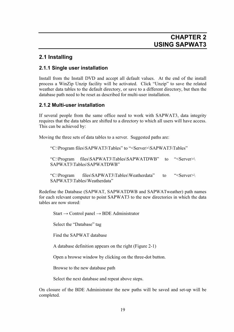
Install from the Install DVD and accept all default values. At the end of the install process a WinZip Unzip facility will be activated. Click “Unzip” to save the related weather data tables to the default directory, or save to a different directory, but then the database path need to be reset as described for multi-user installation.
2.1.2 Multi-user installation
If several people from the same office need to work with SAPWAT3, data integrity requires that the data tables are shifted to a directory to which all users will have access. This can be achieved by: Moving the three sets of data tables to a server. Suggested paths are:
“C:\Program files\SAPWAT3\Tables” to “<Server>\SAPWAT3\Tables” “C:\Program files\SAPWAT3\Tables\SAPWATDWB” to “<Server>\ SAPWAT3\Tables\SAPWATDWB” “C:\Program files\SAPWAT3\Tables\Weatherdata” to “<Server>\ SAPWAT3\Tables\Weatherdata”
Redefine the Database (SAPWAT, SAPWATDWB and SAPWATweather) path names for each relevant computer to point SAPWAT3 to the new directories in which the data tables are now stored:
Start → Control panel → BDE Administrator Select the “Database” tag Find the SAPWAT database A database definition appears on the right (Figure 2-1) Open a browse window by clicking on the three-dot button. Browse to the new database path Select the next database and repeat above steps.
On closure of the BDE Administrator the new paths will be saved and set-up will be completed.

20
Figure 2-1 The BDE Administrator database set-up screen
2.1.3 System requirements
SAPWAT3 requires 1 Gb (see page 64) for program files in the C:\Program files directory and at least 12 GB in the directories where the data sets will be situated.
2.1.4 Data security and reinstallation
On reinstallation existing data files are not overwritten as a means of retaining existing data. Since the distribution of the first Beta versions for testing, some data tables have been changed. People who have received Beta versions before January 2009 for testing need to physically delete all SAPWAT3 data tables before installing new versions, otherwise run-time errors will occur. In single user situations these data tables can usually be found under the C:\Program files\SAPWAT3\Tables directory.
2.2 Introduction to the program
At start-up SAPWAT3 displays the screen shown in Figure 2-2. Figure 2-2, as well as the screen figures that follow, are annotated for a better understanding of the user interfaces.

21
Figure 2-2 The SAPWAT3 Opening screen
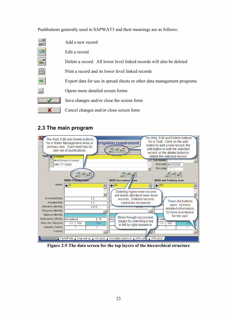
The structure of SAPWAT3 is shown in Figure 2-3 and the data structure is shown in Figure 2-4. Its data structure is relationally organised in hierarchical levels so that the user can add, edit or delete lower level data without breaking the thread that keeps a set of data organised as a unit. The first four layers after the task level, are linkages into higher hierarchy levels that organise data on primary, secondary, tertiary and quaternary drainage regions, or on water management areas, water user association areas, water user association sub-areas and farms, or whatever other four-tier system the user wishes to apply. The main reason behind this structure is that lower level data can be added, edited or deleted whenever required to eventually build a complete picture of a drainage region. The top layer of the structure, Task, fulfils the role of a container that links all related lower level data into a single unit.

22
Figure 2-3 Diagrammatic layout of SAPWAT3 structure
Figure 2-4 The relational organisation of data in SAPWAT3
Outside weather data customised to suit Sapwat3 weather data
tables for importation
Sapwat3 weather data tables
ET0
calculator
Fit ET0 curvilinear regression
Crop data Sapwat3 calculator
Data storageShow water balances on all levels
Enterprise budget(Semi-detailed)
Enterprise budget(Minimum detail)
Enterprise budget calculator
Irrigation system data
Soil data
WMA WUA WUA-sub Farm Crop
Farmer detailWater harvest calculator
Enterprise budget(Fully detailed)
Country data
23
Pushbuttons generally used in SAPWAT3 and their meanings are as follows:
Add a new record
Edit a record
Delete a record. All lower level linked records will also be deleted
Print a record and its lower level linked records
Export data for use in spread sheets or other data management programs
Opens more detailed screen forms
Save changes and/or close the screen form
Cancel changes and/or close screen form
2.3 The main program
Figure 2-5 The data screen for the top layers of the hierarchical structure

24
Figure 2-6 More on the data screen for the top layers of the hierarchical structure
Figure 2-7 The task add/edit screen

25
Figure 2-8 The farm/field screen
Figure 2-9 The farm edit screen
26
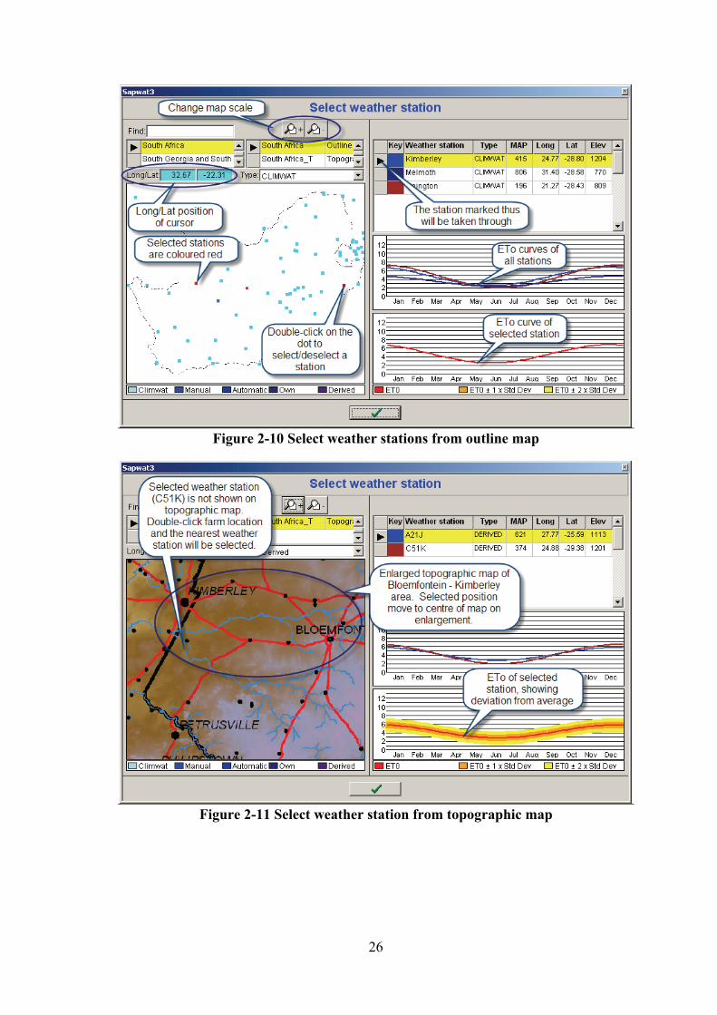
Figure 2-10 Select weather stations from outline map
Figure 2-11 Select weather station from topographic map

27
Figure 2-12 More on the Farm/Field screen
Figure 2-13 The field edit screen
28
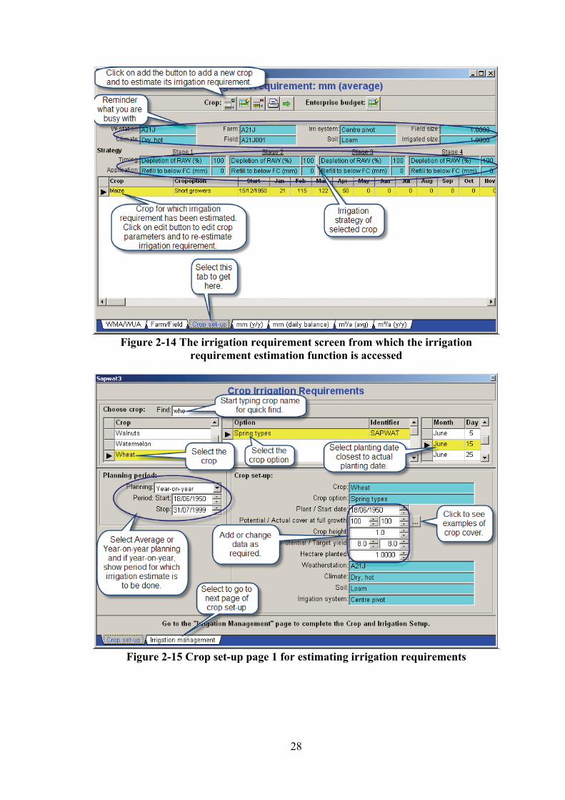
Figure 2-14 The irrigation requirement screen from which the irrigation
requirement estimation function is accessed
Figure 2-15 Crop set-up page 1 for estimating irrigation requirements

29
Figure 2-16 Crop set-up page 2 for estimating irrigation requirements
Figure 2-17 Crop set-up page 2 after completion of crop irrigation estimates
showing results

30
Figure 2-18 Irrigation requirement estimate results with median and percentile
deviation graph
Figure 2-19 Irrigation requirement estimate results with average and standard
deviation graph

31
Figure 2-20 Year on year of ET0 and ETc results
Figure 2-21 Year on year results of irrigation, irrigation loss, rain, rain loss and evaporation results

32
Figure 2-22 The daily water balance table for wheat for the 1950 season
Figure 2-23 A new crop added to the crop irrigation requirement table
33
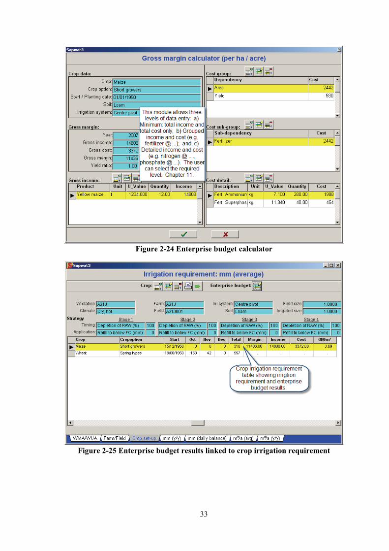
Figure 2-24 Enterprise budget calculator
Figure 2-25 Enterprise budget results linked to crop irrigation requirement

34
Figure 2-26 Changing crop area
Figure 2-27 Opening the water harvest module

35
Figure 2-28 Water harvest module set-up page
Figure 2-29 Graphic representation of monthly water harvest balances

36
Figure 2-30 Water harvest water balance detail
2.4 The menu items
Figure 2-31 Menu access to data used by SAPWAT3

37
2.4.1 Estimate irrigation requirements
This menu item returns the user to the opening screen.
2.4.2 Irrigation systems (refer to Chapter 10)
Figure 2-32 The irrigation systems screen form
2.4.3 Distribution systems and efficiencies (refer to Chapter 10)
Figure 2-33 Distribution systems and efficiencies screen form

38
2.4.4 Soil (refer to Chapter 5)
Figure 2-34 The soil screen form

39
2.4.5 Weather stations (refer to Chapter 4)
Figure 2-35 List of weather stations included from which a station can be selected
Figure 2-36 Weather station detail

40
Figure 2-37 Weather station monthly average data
Figure 2-38 Weather station daily data
41
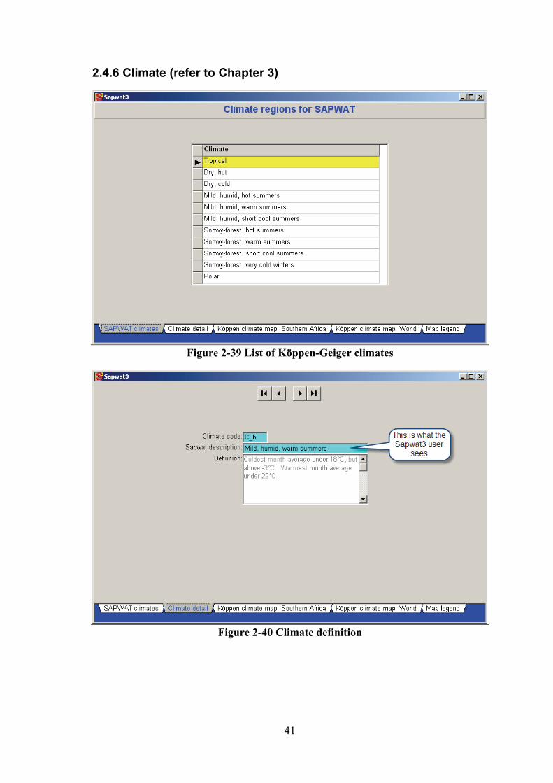
2.4.6 Climate (refer to Chapter 3)
Figure 2-39 List of Köppen-Geiger climates
Figure 2-40 Climate definition
42
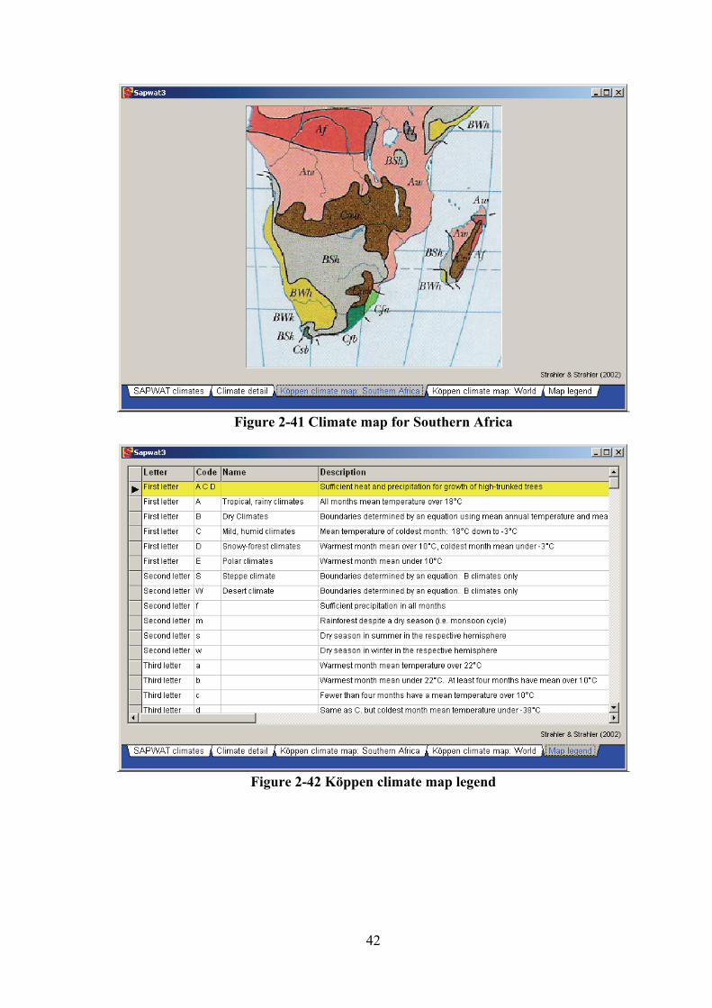
Figure 2-41 Climate map for Southern Africa
Figure 2-42 Köppen climate map legend
43
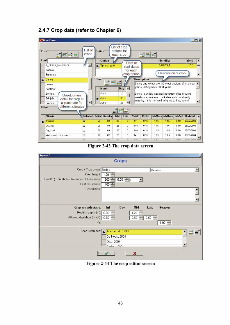
2.4.7 Crop data (refer to Chapter 6)
Figure 2-43 The crop data screen
Figure 2-44 The crop editor screen

44
2.4.8 Crop groups
Figure 2-45 The crop group editor screen
2.4.9 Countries (refer to Chapter 13)
Figure 2-46 A country edit screen

45
2.4.10 Address list
Figure 2-47 The screen form for building a list of addressees

46
CHAPTER 3 CLIMATE
3.1 Introduction
Weather is the immediate day-to-day local combination of such natural phenomena as temperature, precipitation, light intensity, wind direction and velocity and relative humidity. In any location these weather factors assume a certain pattern, changing day-by-day, week-by-week, month-by-month and season-by-season. And the same pattern repeats year by year. This pattern is a location’s climate. Past climate records allow one to predict with some accuracy the weather of a given area for a certain time of the year, and using knowledge of crops, also predict which crops can be grown successfully where and what production practices need to be followed to reduce the risk of partial or complete crop losses (McMahon et al., 2002). Weather data enables one to calculate monthly and annual water balances for an area in order to determine if irrigation would be necessary and how much irrigation would be required. The major influencing elements of a water balance in a soil of an area are the addition of water through rain and the loss of water through evapotranspiration and runoff. Evapotranspiration is the combination of transpiration by the plant and evaporation from a wet surface. The weather parameters of climate that determine the rate of evapotranspiration are temperature, wind and humidity; temperature itself being the result of solar energy reaching the area. Temperature, wind and humidity, as well as rain are parameters of climate; therefore climate can be seen as the basic engine that drives the elements that determine the water balance of an area and therefore of a crop grown in an area. For the application of the FAO four-stage crop growth approach as described by Allen et al. (1998), it is necessary that a fairly accurate determination of the length of each of these cycles be made. CROPWAT (Smith, 1992) and Allen et al. (1998) provides ranges within which these periods could be determined for each site, but the problem is that the user must have a fairly good knowledge of crop reaction to climate in order to make the necessary adaptations to included data. Another problem encountered with the CROPWAT approach is that, although a range of planting dates is implied, the effect of different planting dates on the stage lengths of the four-stage crop growth model is not directly indicated. Once again, the user must rely on his or her local knowledge to adjust stage lengths to suit local conditions. The present SAPWAT has tried to overcome this problem by including in its tables the values and changes in values, reflected by different climatic conditions and also different planting times (Crosby and Crosby, 1999). A problem encountered here was that the database had to be increased substantially to accommodate the seven major geographic and, by implication, climate regions identified for the South African situation as a set of growth stage periods had to be determined for each of these areas. However, it soon became apparent that one could possibly reduce the number of climatic areas by reclassifying these into warmer and colder areas, as average
47
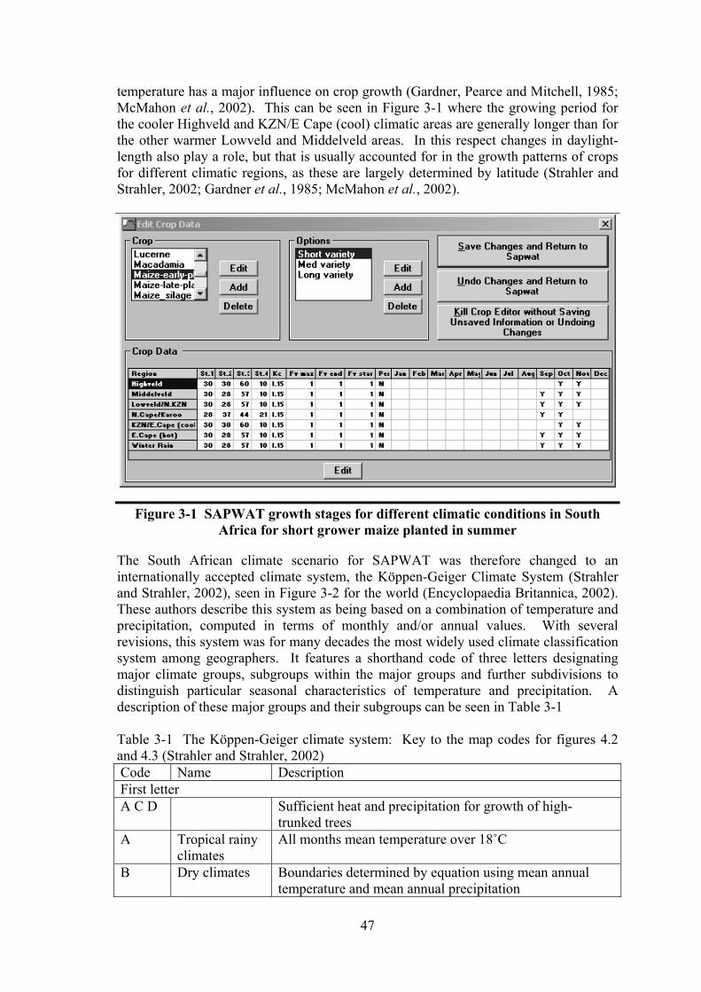
temperature has a major influence on crop growth (Gardner, Pearce and Mitchell, 1985; McMahon et al., 2002). This can be seen in Figure 3-1 where the growing period for the cooler Highveld and KZN/E Cape (cool) climatic areas are generally longer than for the other warmer Lowveld and Middelveld areas. In this respect changes in daylight-length also play a role, but that is usually accounted for in the growth patterns of crops for different climatic regions, as these are largely determined by latitude (Strahler and Strahler, 2002; Gardner et al., 1985; McMahon et al., 2002).
Figure 3-1 SAPWAT growth stages for different climatic conditions in South Africa for short grower maize planted in summer
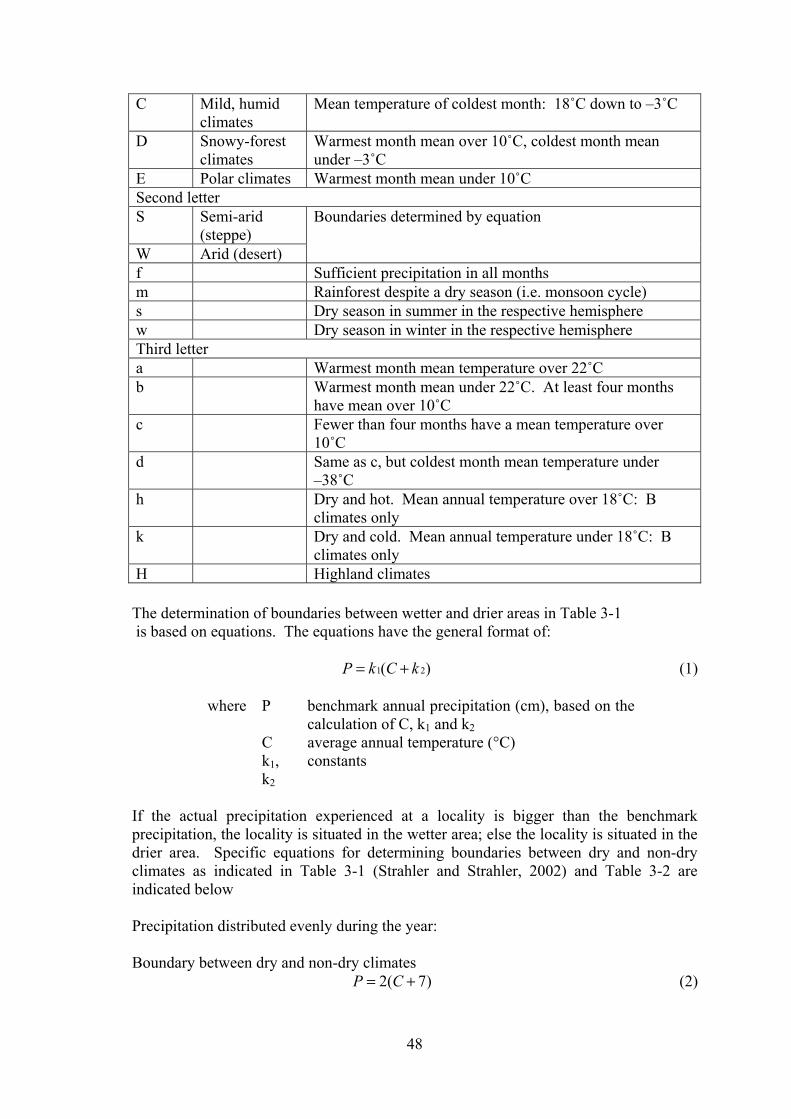
The South African climate scenario for SAPWAT was therefore changed to an internationally accepted climate system, the Köppen-Geiger Climate System (Strahler and Strahler, 2002), seen in Figure 3-2 for the world (Encyclopaedia Britannica, 2002). These authors describe this system as being based on a combination of temperature and precipitation, computed in terms of monthly and/or annual values. With several revisions, this system was for many decades the most widely used climate classification system among geographers. It features a shorthand code of three letters designating major climate groups, subgroups within the major groups and further subdivisions to distinguish particular seasonal characteristics of temperature and precipitation. A description of these major groups and their subgroups can be seen in Table 3-1 Table 3-1 The Köppen-Geiger climate system: Key to the map codes for figures 4.2 and 4.3 (Strahler and Strahler, 2002) Code Name Description First letter A C D Sufficient heat and precipitation for growth of high-
trunked trees A Tropical rainy
climates All months mean temperature over 18˚C
B Dry climates Boundaries determined by equation using mean annual temperature and mean annual precipitation
48
C Mild, humid climates
Mean temperature of coldest month: 18˚C down to –3˚C
D Snowy-forest climates
Warmest month mean over 10˚C, coldest month mean under –3˚C
E Polar climates Warmest month mean under 10˚C Second letter S Semi-arid
(steppe) Boundaries determined by equation
W Arid (desert) f Sufficient precipitation in all months m Rainforest despite a dry season (i.e. monsoon cycle) s Dry season in summer in the respective hemisphere w Dry season in winter in the respective hemisphere Third letter a Warmest month mean temperature over 22˚C b Warmest month mean under 22˚C. At least four months
have mean over 10˚C c Fewer than four months have a mean temperature over
10˚C d Same as c, but coldest month mean temperature under
–38˚C h Dry and hot. Mean annual temperature over 18˚C: B
climates only k Dry and cold. Mean annual temperature under 18˚C: B
climates only H Highland climates
The determination of boundaries between wetter and drier areas in Table 3-1 is based on equations. The equations have the general format of: 1 2( )P k C k (1)
where P benchmark annual precipitation (cm), based on the calculation of C, k1 and k2
C average annual temperature (°C) k1,
k2 constants
If the actual precipitation experienced at a locality is bigger than the benchmark precipitation, the locality is situated in the wetter area; else the locality is situated in the drier area. Specific equations for determining boundaries between dry and non-dry climates as indicated in Table 3-1 (Strahler and Strahler, 2002) and Table 3-2 are indicated below Precipitation distributed evenly during the year: Boundary between dry and non-dry climates 2( 7)P C (2)

49
Between steppe and desert climates 7P C (3)
Precipitation concentrated in summer: Boundary between dry and non-dry climates 2( 14)P C (4)
Between steppe and desert climates 14P C (5)
Precipitation concentrated in winter: Boundary between dry and non-dry climates 2P C (6)
Between steppe and desert climates P C (7)
Figure 3-2 Köppen-Geiger climate map of the world (Encyclopaedia Britannica,
1994)
3.2 Application in SAPWAT3
Because the Köppen-Geiger climate system is based on temperature-rainfall combinations, the climate of a weather station can be determined by using the temperature and rainfall data of a weather station record. This fits into the SAPWAT3 concept, where weather station data is used as a basis for estimating crop water requirements. One adaptation was made, that is that the second letter of the three-letter Köppen-Geiger code, which indicates rainfall seasonality, is not used because rainfall seasonality is superseded by irrigation scheduling. The result, for inclusion in the SAPWAT3 climate data table can be seen in Table 3-2. The user will not be confronted with climate codes; what the user will see is the description shown in column 7 of Table 3-2. The definitions of the different climatic regions are available in the Climate data table that is included in SAPWAT3.

50
Table 3-2 Table showing the adaptation of the Köppen-Geiger climate system for
SAPWAT3 purposes Köppen climate codes
SAPWAT3 data table codes
Tavg Tmax Tmin Months with Tavg > 10C
Name of SAPWAT3 climate
Af, Am, Aw
A_ >18 12 Tropical
BSh, BWh B_h >18 >4 Dry, hot BSk, BWk B_k =<18 >4 Dry, cold Cfa, Csa, Cwa
C_a >22 >-3 >4 Mild, humid, hot summers
Cfb, Csb, Cwb
C_b =<22 >-3 >4 Mild, humid, warm summers
Cfc, Csc, Cwc
C_c =<22 >-3 =<4 Mild, humid, cool summers
Dfa, Dsa, Dwa
D_a >22 =<-3, >-38
>4 Snow, hot summers
Dfb, Dsb, Dwb
D_b =<22 =<-3, >-38
>4 Snow, warm summers
Dfc, Dsc, Dwc
D_c =<22 =<-3, >-38
=<4 Snow, cool summers
Dfd, Dsd, Dwd
D_d =<22 =<-38 =<4 Snow, very cold winters
ET, EF E_ =<10 =<4 Polar
3.2.1 Data organisation
The data is stored in a single data table that acts as a lookup table for SAPWAT3. As this data is based on internationally accepted defined parameters, the user can access the data as read-only.
51
CHAPTER 4 WEATHER STATIONS
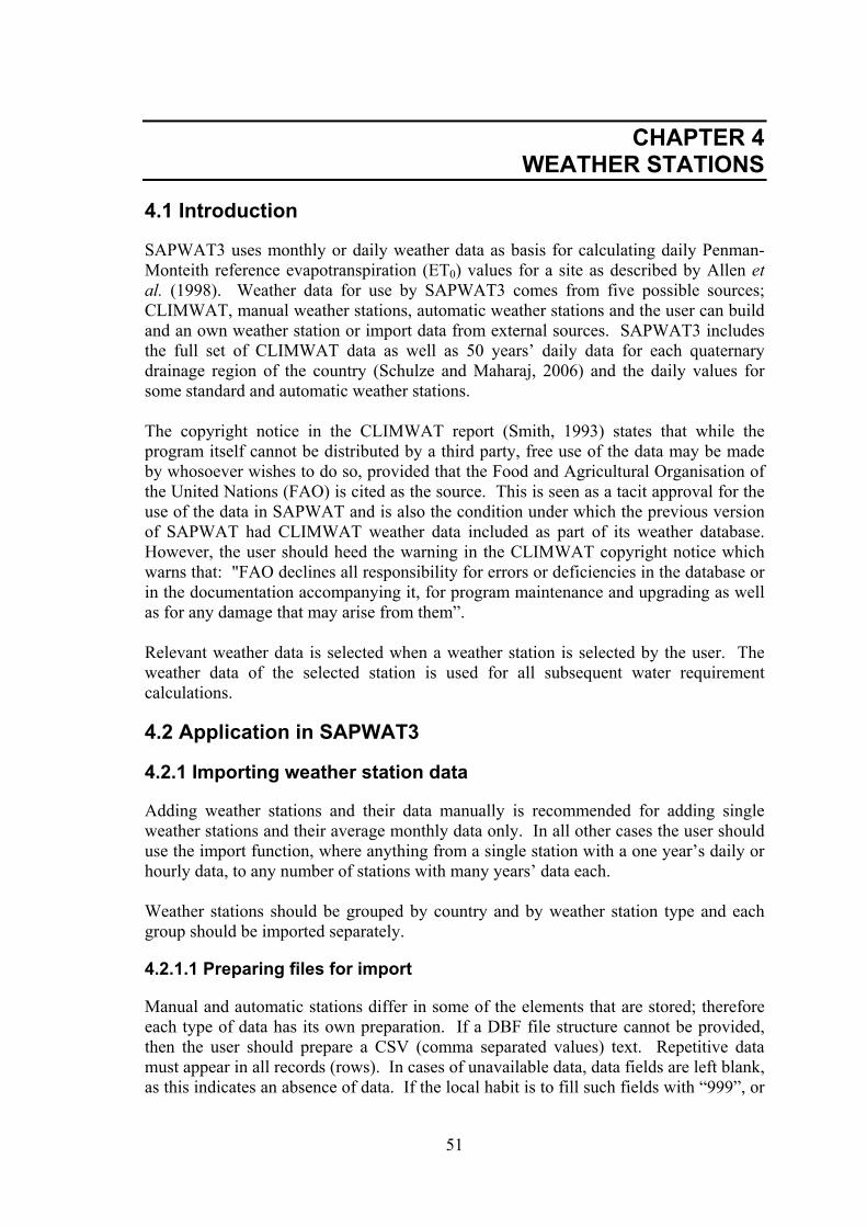
4.1 Introduction
SAPWAT3 uses monthly or daily weather data as basis for calculating daily Penman-Monteith reference evapotranspiration (ET0) values for a site as described by Allen et al. (1998). Weather data for use by SAPWAT3 comes from five possible sources; CLIMWAT, manual weather stations, automatic weather stations and the user can build and an own weather station or import data from external sources. SAPWAT3 includes the full set of CLIMWAT data as well as 50 years’ daily data for each quaternary drainage region of the country (Schulze and Maharaj, 2006) and the daily values for some standard and automatic weather stations. The copyright notice in the CLIMWAT report (Smith, 1993) states that while the program itself cannot be distributed by a third party, free use of the data may be made by whosoever wishes to do so, provided that the Food and Agricultural Organisation of the United Nations (FAO) is cited as the source. This is seen as a tacit approval for the use of the data in SAPWAT and is also the condition under which the previous version of SAPWAT had CLIMWAT weather data included as part of its weather database. However, the user should heed the warning in the CLIMWAT copyright notice which warns that: "FAO declines all responsibility for errors or deficiencies in the database or in the documentation accompanying it, for program maintenance and upgrading as well as for any damage that may arise from them”. Relevant weather data is selected when a weather station is selected by the user. The weather data of the selected station is used for all subsequent water requirement calculations.
4.2 Application in SAPWAT3
4.2.1 Importing weather station data
Adding weather stations and their data manually is recommended for adding single weather stations and their average monthly data only. In all other cases the user should use the import function, where anything from a single station with a one year’s daily or hourly data, to any number of stations with many years’ data each. Weather stations should be grouped by country and by weather station type and each group should be imported separately.
4.2.1.1 Preparing files for import
Manual and automatic stations differ in some of the elements that are stored; therefore each type of data has its own preparation. If a DBF file structure cannot be provided, then the user should prepare a CSV (comma separated values) text. Repetitive data must appear in all records (rows). In cases of unavailable data, data fields are left blank, as this indicates an absence of data. If the local habit is to fill such fields with “999”, or

52
whatever, it should be replaced with a blank, because any data in a field is seen as a data entry and such entries could lead to surprising results. Any number of weather stations can be included in an import data file. However, there is a file size limit of 650 Mb for DBF and 400 Mb for CSV files for successful importation and manipulation. It is essential to note which fields in the import file must contain data (Table 4-1 and Table 4-2). The absence of data in any of these fields will result in the abortion of the importation routine.
4.2.1.1.1 Manual station data Table 4-1 shows the required structure for the importation of manual weather station data into SAPWAT3.
Table 4-1 Prepared data table structure for importation of manual weather station into SAPWAT3
Field name Data type Field width
Decimals Remarks
WSFilename Character 9 The locally used file name or file reference for a particular station, e.g., 345671, GB54370WD. Must be included and must be unique.
Wstation Character 40 Weather station common name, e.g. Jonestown. Must be unique for each type of station per country. Must be included.
Longitude Numeric 9 4 Degrees decimal, longitude west is shown as negative. Must be included.
Latitude Numeric 9 4 Degrees decimal, latitude south is shown as negative. Must be included.
Elevation Numeric 6 0 Height above sea level in meters. Must be included.
Yearsdata Numeric 4 0 Number of years of records included. rDate Date 8 Record date in mm/dd/yyyy format.
Date or (Year and DOY). Must be included.
rYear Numeric 4 0 Year. Date or (Year and DOY) must be included.
DOY Numeric 3 0 The Day of Year, with January 1 being DOY 1. Date or (Year and DOY) must be included
rTime Numeric 4 0 Daily time of weather station visit, in 24 hour format, e.g. 0700 for seven in the morning.
Tmax Numeric 6 1 Maximum temperature (°C). Must be included
Tmin Numeric 6 1 Minimum temperature (°C). Must be included
Hmax Numeric 6 1 Maximum humidity (%). Hmin Numeric 6 1 Minimum humidity (%). Program
estimates this value if omitted. Should

53
preferably be included. Havg Numeric 6 1 Average humidity (%). Program
estimates this value if omitted. Wind Numeric 4 1 Average m s-1. Program uses default of 2
m s-1 if omitted. Windrun Numeric 6 1 Wind distance for day (Km). Program
calculates from default, if omitted. Sunshine Numeric 4 1 Hours of sunshine. One of Sunshine or
Radiation or RadWatt must be included. Radiation Numeric 5 1 Average radiation (MJ m-2 day-1). One
of Sunshine or Radiation or RadWatt must be included.
RadWatt Numeric 8 3 Average radiation (Watts m-2). Not normally part of daily data, but seems to be included in some cases. One of Sunshine or Radiation or RadWatt must be included.
Rain Numeric 6 1 mm. Should be included.
4.2.1.1.2 Automatic station data Table 4-2 shows the required structure for the importation of automatic weather station data into SAPWAT3.
Table 4-2 Prepared data table structure for importation into SAPWAT Field name Data type Field
widthDecimals Remarks
WSFilename Character 9 The locally used file name or file reference for a particular station, e.g., 345671, GB54370WD. Must be included and must be unique.
Wstation Character 40 Weather station common name, e.g. Jonestown. Must be unique for each type of station per country. Must be included
Longitude Numeric 9 4 Degrees decimal, longitude west is shown as negative. Must be included
Latitude Numeric 9 4 Degrees decimal, latitude south is shown as negative. Must be included
Elevation Numeric 6 0 Height above sea level in meters. Must be included
Yearsdata Numeric 4 0 Number of years of records included. rDate Date 8 Record date in mm/dd/yyyy format. Date or
(Year and DOY) must be included. rYear Numeric 4 0 Year. Date or (Year and DOY) must be
included. DOY Numeric 3 0 The Day of Year, with January 1 being
DOY 1. Date or (Year and DOY) must be included.
rTime Numeric 4 0 Time of data record, in 24 hour format, e.g. 0700 for seven in the morning.

54
Temperature Numeric 6 1 Average temperature of recording period (°C). Must be included.
Humidity Numeric 6 1 Average humidity of recording period (%). Program estimates of omitted.
Wind Numeric 4 1 Average m s-1. Program uses default of 2 m s-1 if omitted.
Sunshine Numeric 4 1 Time during recording period. One of Sunshine or Radiation or RadWatt must be included.
Radiation Numeric 5 1 Average radiation for period (MJ m-2). One of Sunshine or Radiation or RadWatt must be included.
RadWatt Numeric 8 3 Average radiation for recording period (Watts m-2). One of Sunshine or Radiation or RadWatt must be included.
Rain Numeric 6 1 mm. Should be included.
4.2.1.1.3 Importing data into the SAPWAT weather station database Once the data has been prepared, it is imported into SAPWAT3. In this process, data is normalised, which in the case of these files, is a split of the import file into a weather station data file and a weather data file. Penman-Monteith ET0 values are calculated for each record. In this process, missing data is calculated or estimated as described by Allen et al. (1998). A regression for ET0 over time (DOY) is calculated and the equation of this curve is added to the weather station data for use in the irrigation requirement calculations. The importation of weather data could take several hours; weather data tables tend to contain many records. One manual weather station with 1 year’s daily entries would contain 365 (366 for a leap year) records. One automatic weather station with 1 year’s hourly entries would contain 8 760 (8 784 for a leap year) records.

55
CHAPTER 5 SOIL
5.1 Introduction
Broadly speaking, soil is defined as unconsolidated inorganic and organic material on the immediate surface of the earth that act as a natural medium for the growth of plants and all other soil-living creatures. It is a mix of solid inorganic particles, water, air and organic material. It is an integral part of the landscape and its characteristics; appearance and distribution is determined by climate, parent material, topography, flora, fauna and time. The parent material accumulates as an unconsolidated mass that later differentiates into characteristic layers called horizons. Differentiation occurs by means of chemical differentiation and/or dissolution of the parent material. As the process continues, the horizons generally become more distinguishable and finally develop into a soil profile (McMahon et al., 2002). Soil can be highly variable in a landscape with observable differences in depth, texture, structure and slope. The effect of differences in chemical content is sometimes obvious and changes can sometimes be predicted for specific land use activities. Not all soils are suitable for irrigation. Irrigation induces changes in the physical, chemical and biological characteristics of a soil; therefore land classification for irrigation should consider the various potential changes and use this as a background for delineating lands on the basis of suitability for irrigation use. Land classification for irrigation should provide a sound basis for fitting land resources into a plan of irrigation development (Maletic and Hutchins, 1967).
5.2 Soil in Irrigation
The irrigator is interested in a soil that can be economically developed, is easy to cultivate, will allow full potential root development, will be chemically suitable for the crops to be grown and will be stable over time (Maletic and Hutchins, 1967). Of special interest to the planner of irrigation water requirement and the scheduling service is the water holding capacity of a soil and the factors that influences it, the ease with which a crop can access that water and the related osmotic forces, the hydraulic conductivity of soil and potential changes that could occur because of irrigation or that can influence irrigation type and strategy over time (Day, Bolt and Anderson, 1967).
5.3 Soil water
A thorough understanding of the soil water balance and the factors that influence it is essential. It can be mathematically described and is diagrammatically represented in Figure 5-1 (Allen et al., 1998; Bennie et al., 1998):

56
DPCRTEROPID )( (8)
Where ΔD Change in soil water content I Irrigation P Precipitation RO Run-off E Soil surface evaporation T Crop transpiration CR Capillary rise DP Deep percolation
Subsurface inflow and outflow in waterlogged or semi-waterlogged situations is not shown, but both situations can be accommodated in a way by capillary rise and deep percolation
Figure 5-1 A diagrammatic representation of the soil water balance in the root
zone of crop (Allen et al., 1998)
Figure 5-1 show that addition of water to a profile as coming from rain, irrigation and capillary rise, while the extraction of water is through evapotranspiration (transpiration and soil surface evaporation) and deep percolation. Runoff from soil surface does not add to the soil water content and is usually subtracted from rainfall. The amount of rainfall, transpiration and soil surface evaporation is linked to the climate of the area, while capillary rise and deep percolation is mainly influenced by water management on the irrigated and surrounding areas. What are also diagrammatically shown are the concepts of:

57
Field capacity The amount of water that a soil can hold after all free water has been allowed to drain out of the root zone
Wilting point The water level in root zone at which plants will be permanently wilted
Depletion The amount of water depleted out of the root zone through evapotranspiration
RAW Readily available water – the amount of water that is available to a crop without the crop undergoing stress situations
TAW Total available water – the total amount of plant available water that a soil can hold in the root zone
5.4 Evaporation from the soil surface
Where the topsoil is wet following a rain or irrigation the evaporation component (KeET0) is at a maximum. As the soil surface becomes drier, soil surface evaporation is reduced until a level of no practically measurable evaporation is reached. Evaporation occurs predominantly from the exposed soil fraction. Hence, evaporation is restricted at any moment by the energy available at the exposed soil fraction; therefore Ke cannot exceed fewKcmax, where few is the fraction of soil from which most evaporation occurs, i.e. the fraction of the soil not covered by vegetation and wetted by irrigation or precipitation (Allen et al., 1998). Evaporation from the soil surface can be assumed to take place in two stages: an energy limiting stage, and a falling rate stage. When the soil surface is wet, Kr (dimensionless evaporation reduction coefficient) is 1. When the water content in the upper soil becomes limiting, Kr decreases and becomes zero when the total amount of water that can be evaporated from the topsoil is depleted (Allen et al., 1998). In the simple evaporation procedure it is assumed that the water content of the evaporation layer of the soil is at field capacity, θFC, shortly following a major wetting event and that the soil can dry to a water content level that is halfway between oven dry (no water left) and wilting point, θWP, The amount of water that can be depleted by evaporation during a complete drying cycle can hence be estimated as (Allen et al., 1998): ZeTEW WPFC )5.0(1000 (9)
Where TEW Total evaporable water = maximum depth of water that can be evaporated from the soil when the topsoil has been initially completely wetted [mm]
θFC Soil water content at field capacity [m3 m-3] θWP Soil water content at wilting point [m3 m-3] Ze Depth of surface soil layer that is subject to drying by way of
evaporation [0.10-0.15 m]. When unknown, a value for Ze, the effective depth of the soil evaporation layer, of 0.1 to 0.15 m is recommended Allen et al. (1988). Typical values for θFC, θWP and TEW are given in Table 5-1 (Allen et al., 1998).

58
Table 5-1: Typical soil water characteristics for different soil types
Soil type Soil water characteristics Evaporation parameters θFC θWP θFC-θWP Amount of water that can be
depleted by evaporation Stage 1 REW
Stage 1 and 2 TEW (Ze = 0.1 m)
m3/m3 m3/m3 m3/m3 mm mm Sand 0.07-0.17 0.02-0.07 0.05- 0.11 2-7 6-12 Loamy sand
0.11-0.19 0.03-0.10 0.06-0.12 4-8 9-14
Sandy loam
0.18-0.28 0.06-0.16 0.11-0.15 6-10 15-20
Loam 0.20-0.30 0.07-0.17 0.13-0.18 8-10 16-22 Silt loam 0.22-0.36 0.09-0.21 0.13-0.19 8-11 18-25 Silt 0.28-0.36 0.12-0.22 0.16-0.20 8-11 22-26 Silt clay loam
0.30-0.37 0.17-0.24 0.13-0.18 8-11 22-27
Silty clay 0.30-0.42 0.17-0.29 0.13-0.19 8-12 22-28 Clay 0.32-0.40 0.20-0.24 0.12-0.20 8-12 22-29
The relationship between REW and TEW is shown in Figure 5-2 (Allen et al., 1988)
Figure 5-2 Soil evaporation reduction coefficient, Kr. The effect of the two stages, the energy limiting stage and the falling rate stage can be seen (Allen et al., 1998)
59
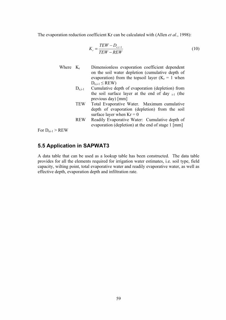
The evaporation reduction coefficient Kr can be calculated with (Allen et al., 1998):
, 1e ir
TEW DK
TEW REW
(10)
Where Kr Dimensionless evaporation coefficient dependent
on the soil water depletion (cumulative depth of evaporation) from the topsoil layer (Kr = 1 when De,i-1 ≤ REW)
De,i-1 Cumulative depth of evaporation (depletion) from the soil surface layer at the end of day i-1 (the previous day) [mm]
TEW Total Evaporative Water. Maximum cumulative depth of evaporation (depletion) from the soil surface layer when Kr = 0
REW Readily Evaporative Water: Cumulative depth of evaporation (depletion) at the end of stage 1 [mm]
For Dei-1 > REW
5.5 Application in SAPWAT3
A data table that can be used as a lookup table has been constructed. The data table provides for all the elements required for irrigation water estimates, i.e. soil type, field capacity, wilting point, total evaporative water and readily evaporative water, as well as effective depth, evaporation depth and infiltration rate.

60
CHAPTER 6 CROPS
6.1 Introduction
Water influences the growth and development of plants because it is essential in every biological reaction within the plant. It is the most abundant constituent in plants, ranging from about 75 to 90 percent of a plant’s mass by weight. The role of water includes: (1) involvement in all biological reactions, (2) a structural component in the proteins and nucleic acids in the plant cells, and (3) a regulator of plant temperature. In addition to its in-plant role, water also acts as an environmental regulator of the climate around the plant. Moisture is a major factor determining climate. It is generally assumed that if adequate rainfall is received during two-thirds of a growing season, the growing season would have enough water for most of the mesophytic crops usually grown by man. Otherwise at least some irrigation is required, although the amount required could vary, especially if a mix of mesophytic and xerophytic plants is included in a crop production system (McMahon et al., 2002). All annual and deciduous crops have a similar growth and development pattern, i.e. new growth starts at the beginning of the season with new foliage developing and very little ground shading. As the crops develop, foliage develops until the soil surface is mostly or fully overshadowed. Plants then usually go into a reproductive phase where seed and fruit are developed. These ripen towards the end of the season, the foliage starts dying and at the end of the season bare ground is again found. A similarity to this pattern is found in perennial evergreen crops grown in non-tropical areas, in the sense that even though the foliage stays intact and active, a slow-down in photosynthesis is usually found during the off-season period of the crops. The problem that has faced the irrigation water requirement planner and designer was how to describe this rather complex physiology and phenology in terms that are easily understood by the not-so-well-trained person while still being credible. This problem was solved by adopting the four-stage growth cycle approach for describing the growth and development of crops (Allen et al., 1998).
6.2 The four-stage crop cycle
SAPWAT3 is based on the same four-stage approach to crop development for estimating crop irrigation water as CROPWAT (Smith, 1992), therefore it seems fitting that a short overview of developments in this field be given here. The report “Guidelines for predicting crop water requirements” by Doorenbos and Pruit, (1977), included two important concepts that had the potential to eliminate some of the shortcomings that were identified in the introduction to the Green Book (Green, 1985). It recognized the limitations of the use of A-pan evaporation and recommended short grass as reference evaporation, in association with the linked and less empirical four-stage approach for the development of crop factors. This reference evaporation is in harmony with the growing plant, so that there is automatic compensation for climatic differences. When full, effective ground cover is reached; the crop factor would be 1.0.

61
The four stages of crop development are described as follows:
Initial stage:
Germination and early growth, when the ground surface is barely covered by the crop (ground cover <10%)
Crop development stage:
From the end of the initial stage to the reaching of effective full ground cover (ground cover 70-80%)
Mid season stage: From reaching full effective ground cover, till the beginning of maturity, as indicated by colour change of leaves and leaf drop
Late season stage: from the end of the mid season stage to full maturity or harvest
The basic approach for the estimation of crop water use is still the same as with A-pan and crop factors: 0*crop cET K ET (11)
where: ETcrop crop evapotranspiration Kc crop coefficient ET0 reference evaporation
The value of ET0 was originally determined with the aid of weighing lysimeters. Different methods for the calculations of these values from climatic data have been developed. These include methods that derive ET0 form A-pan evaporation (E0). Eventually the Penman-Monteith equation for the calculation of ET0 has been internationally recognized and has been published as the standard calculation method in the FAO Irrigation and Drainage Report No 56 (Allen et al., 1998). Smith (1991) reported on the expert consultation with the aim of evaluating FAO No 24 that took place in Rome during 1990:
In the series of Irrigation and Drainage reports the FAO methodology for the estimation of crop water requirements has proved itself as exceptional. FAO 24 became the international standard, and irrigation engineers, agronomists, hydrologists and environmentalists are using it on a worldwide scale. More than 200 000 copies have already been distributed in four languages. FAO 24 was combined with FAO Irrigation and Drainage Report No 33 “Yield responses to water” (Doorenbos, Kassam, Bentvelsen, Bransheid, Plusjé, Smith, Uittenbogaard and Van der Wal, 1986), and was published as a computer program CROPWAT (Smith, 1992). This program further enhanced the acceptance of the FAO procedures. The consultation decided that crop factors are still valid, but that updating is justified and that the following should be considered:
Review, with specific reference, crop factors for trees and fruit crops, as well as several of the perennial crops; Review crop factors, specifically during the initial stage, by evaluating soil evaporation and basal crop transpiration separately;

62
Review the effect of climate and advective conditions on the crop factor; Review and update the length of the different growth stages, possibly also the incorporation of a growth function coupled to temperature and dry matter yield.
Since the consultation progress has been made on these aspects. Recommended procedures and data are published in FAO Irrigation and Drainage Report No 56 (Allen et al., 1998). As far as is known, this progress has not yet been directly integrated into design and planning programs. Smith (1994) strongly recommended that the four-stage FAO procedure for the determination of crop factors be applied in SAPWAT to ensure a transparent and internationally comparable methodology. He acknowledges that the standard crop factors has to be adjusted to provide for the climatic conditions of regions, new cultivars, deviations in planting density as well as for the full range of irrigation methods. One of the shortcomings of similar programs is that they were designed in the days of long cycle flood and sprinkler irrigation and thus do not reflect techniques applied by developing farmers, such as wide spaced, short row, surface irrigation. The need for the separate evaluation of soil evaporation and plant transpiration has been identified during the expert consultation (Smith, 1991), and a recommended methodology was published later (Allen et al., 1996). At about the same time a similar procedure was developed for SAPWAT, based on the work done by De Jager and Van Zyl (1987) and by Strooisnijder (1987). The SAPWAT procedure has the advantage that it is independent of soil texture. If the soil evaporation and plant transpiration is considered, it becomes possible to manipulate the basic crop factors to provide for ground cover, wetted area, frequency of irrigation, cover crops, fruit trees, perennial crops, and different irrigation systems. SAPWAT was the first program that applied this possibility in a user orientated crop irrigation program. A lot of attention needs to be given to crop factor values, specifically peak values. There is a tendency to accept the default crop factor curve or table as a given physiological characteristic of a crop. Nothing is further from the truth. Unrealistic or incorrectly applied crop factors are probably the main reason for inaccurate estimates of irrigation requirements. During the development of SAPWAT, specific attention was given to crop factors. The ideal would have been to let the crop grow, similar to growth models, so that stage length will react to planting date and climate. However, this is not possible in a program of this nature, because of the comprehensive inputs required to simulate crop growth. The use of short grass reference evaporation reduces the impact of climatic change on crop water use, but has no influence on the length of growth stages. The solution was to subdivide South Africa into seven agro-climatic regions and to develop default crop factors for each of these regions. Default planting dates for each region and crop is also specified and where planting date has a noticeable influence on growth stages, individual crop files were developed according to planting month per region. Where noticeable differences between cultivars (e.g. early or late) are found, each is handled as a separate crop. The crop factor file was developed according to rules derived with the help of crop scientists. Validation of these values takes place continuously and is based on practices in the field and on the experience of irrigation consultants. The default crop factor files provide for manipulations as discussed. The
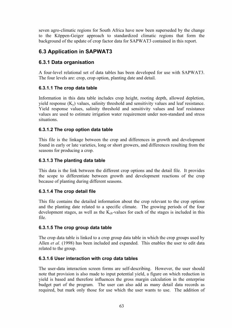
63
seven agro-climatic regions for South Africa have now been superseded by the change to the Köppen-Geiger approach to standardized climatic regions that form the background of the update of crop factor data for SAPWAT3 contained in this report.
6.3 Application in SAPWAT3
6.3.1 Data organisation
A four-level relational set of data tables has been developed for use with SAPWAT3. The four levels are: crop, crop option, planting date and detail.
6.3.1.1 The crop data table
Information in this data table includes crop height, rooting depth, allowed depletion, yield response (Ky) values, salinity threshold and sensitivity values and leaf resistance. Yield response values, salinity threshold and sensitivity values and leaf resistance values are used to estimate irrigation water requirement under non-standard and stress situations.
6.3.1.2 The crop option data table
This file is the linkage between the crop and differences in growth and development found in early or late varieties, long or short growers, and differences resulting from the seasons for producing a crop.
6.3.1.3 The planting data table
This data is the link between the different crop options and the detail file. It provides the scope to differentiate between growth and development reactions of the crop because of planting during different seasons.
6.3.1.4 The crop detail file
This file contains the detailed information about the crop relevant to the crop options and the planting date related to a specific climate. The growing periods of the four development stages, as well as the Kcb-values for each of the stages is included in this file.
6.3.1.5 The crop group data table
The crop data table is linked to a crop group data table in which the crop groups used by Allen et al. (1998) has been included and expanded. This enables the user to edit data related to the group.
6.3.1.6 User interaction with crop data tables
The user-data interaction screen forms are self-describing. However, the user should note that provision is also made to input potential yield, a figure on which reduction in yield is based and therefore influences the gross margin calculation in the enterprise budget part of the program. The user can also add as many detail data records as required, but mark only those for use which the user wants to use. The addition of

64
references linked to records is handy, as has been found that information regarding crop growth and development vary amongst sources. A possible controversial adaptation has been incorporated in the crop data. The mid-season growth stage has been given two entries, a start and an end entry. This allows the user to add different values for the start and end of this stage so that a slope can be added to the midseason. This adaptation is based on observations of results in mainly tree crops with long midseason periods, and specifically those which cross seasonal boundaries, where it has been observed that if a slight slope is given to the midseason stage line, a set of monthly irrigation requirements is estimated which is closer to actual values found than the existing output where the midseason stage line is parallel to the x-axis. The user can add any number of data at any of the levels. The maximum file size for each of these files is 2 Gb or 1 * 109 records, whichever limit is reached first. It is possible that system limitations might reduce these maxima. Crop characteristics are included in the data tables for crops usually grown in the A (tropical), B (dry) and C (mild) climate zones. Climates D (snow) and E (ice) are included in the climate data table; therefore a user could add crops grown in any climate region.
6.4 Methodology
Crop characteristics for application by SAPWAT were mainly collected by means of surveys of researchers, technicians and farmers who grow the crops and, where possible, evaluated against existing published data. One of the unfortunate things about the four-stage FAO crop factor curve is that the data required to apply it, is not necessarily included in the data that researchers usually collect. The usual pattern of data collection related to growth and development is that of planting day, day of emergence, commencement of flowering / tasseling / earing, day when the crop is physiologically ripe, reaping dates and production levels. The four-stage curve required dates of planting, 10% foliage cover, 70% to 80% foliage cover (usually when leaf area index (LAI) reaches about 3), beginning of senescence (first signs of the discolouration of leaves), last day of irrigation, the last day of growth and level of activity when growth stops (Allen et al., 1998). As some of these events occur in between those that are usually noted, one has to rely on the observation capacity of the researcher, technician and farmer to deduce applicable dates or periods for the stages of the four-stage growth curve. This task can be approached in several ways, one of which is to visit knowledgeable scientists, scheduling consultants and farmers in different irrigation areas and to reproduce what they are doing in practice in the field with SAPWAT simulations. This is successful where there is data available as was the case in the Orange-Riet and Orange-Vaal river areas through the offices of the Orange-Vaal and Orange-Riet WUAs and of GWK Ltd (Van Heerden et al., 1999). What has come out of this work is that ways and means of undertaking field checks on “what is going on” under the soil surface is an important aspect of verifying crop coefficients. Only too often this information is not available. The list of personal communications for this purpose is taken up in the source list. The data thus collected is compared to data published in FAO 56 (Allen et al., 1998) and

65
related literature. The four-stage crop coefficient curve, its influence on crop irrigation requirements, soil water balances and irrigation strategies were reviewed. This led to the confirmation or adaptation of the crop characteristics of those crops included in the SAPWAT3 data files: Bananas: Morse, Robinson and Ferreira, 1996. Chicory: Aucamp, 1978; Luckman, 2002. Citrus and Subtropical crops: Childs, 2002; Van Rensburg, 2004; Du Preez, 2003; Tolmay and Kruger, undated. Cotton: Sentrale Katoenkoöperasie, Undated. Dates: Ziad, 1999. Deciduous fruit: Volschenk et al., 2003; North, 2004. Field crops: Booyens, 2004; Ceronio, 2004; De Jager, 1994; Du Plessis, 2003; Gerber, 2003; McMahon et al., 2002; Nel, 2003; Otto, 2004; Van Heerden et al., 1999; Smit, 2003; Van der Schyff, 2004; Viviers, 2003; Wilken, 2004. Fodder crops and Pastures: De Kock, 2004; Dickinson and Hyam (Ed), 1984; Marais et al., 2002; Meredith, 1959; Theron, 2002. Grapes: Albertse 2004; Myburgh, 2004a; Myburgh, 2004b; Myburgh and Howell, 2007a; Myburgh and Howell, 2007b. Groundnuts: Jansen, 2004. Irrigation scheduling, soil water balance and crop reaction: Annandale et al., 1999; Bennie et al., 1998; Bennie et al., 1997; Crosby and Crosby, 1999; De Jager et al., 2001; Doorenbos et al., 1986; Garg, 1992; Hagan et al., 1967; Hoffman, 2004; LeCler, 2004; Smith, 1992; Van Heerden et al., 1999. Irrigation systems and adaptation to crops: Hoffman et al., 1990; Sanmugnathan et al., 2000; USWRC, 1976. Oil seeds: Liebenberg, 2002. Olives: Netafim Agricultural Section, 2002. Potatoes: Coetzee, 2004; Steyn, 2004. Sugar Beet: Cooke and Scott, 1993. Sugar cane: Inman-Bamber and McGlinchey, 2003; Olivier, 2004. Tobacco: Dippenaar, 2003.

66
Vegetables: Annandale et al., 1996; Jovanovic and Annandale, 1999; McMahon et al., 2002; Mappledoram, 2004; Reader’s Digest, 1984; Van Heerden et al., 1999; Van Wyk, 1992.
6.4.1 Possible improvements
The present system, where a four stage crop growth curve is drawn for each combination of crop, crop option, planting date and climate, is time consuming and many records are generated which increases the possibility of errors. This leads one to agree with Allen et al. (1998), that different approaches of constructing a crop growth curve need to be investigated. One of the possibilities is the construction of a basic curve and possible mathematical or statistical adjustments of that basic curve to reflect changes due to heat units, cold units, daylight length and whatever other combination of climatic parameter that could influence crop growth and development. However, it was found during surveys on crop growth and development that the responder could very easily link into the concept of the four-stage approach and could in most cases, give usable answers. The fourth stage curve is also very easy to adapt, if the need should arise.

67
CHAPTER 7 EVAPOTRANSPIRATION
7.1 Factors affecting evapotranspiration
Weather parameters, crop characteristics, management and environmental aspects are factors that affect transpiration and evaporation. The related concepts are shown in Figure 7-1 (Allen et al., 1998).
Figure 7-1: Factors affecting evapotranspiration with reference to related ET
concepts (Allen et al., 1998)
The principle weather parameters affecting evapotranspiration are radiation, air temperature, humidity and wind speed. Several procedures have been developed to assess the evaporation rate from these parameters. The evaporative power of the atmosphere is expressed by the reference crop evapotranspiration (ET0) which represents the evapotranspiration from standardised vegetation. The crop type, variety and development stage should be considered when assessing the evapotranspiration from crops grown in large, well managed fields. Differences in resistance to transpiration, crop height, crop roughness, reflection, ground cover and crop rooting characteristics result in different ET levels in different types of crops under identical environmental conditions. Crop evapotranspiration under standard conditions (ETc) is the evapotranspiration demand from crops that are grown in large fields under optimum soil water, excellent management and environmental conditions, and achieve full production under the given climatic conditions (Allen et al., 1998). Factors such as soil salinity, poor land fertility, and limited application of fertilizers, the presence of hard or impenetrable soil horizons, the absence of control of diseases and pests and poor soil management may limit the crop development and reduce the

68
evapotranspiration. Other factors to be considered when assessing ET are ground cover, plant density and soil water content. The effect of soil water content on ET is conditioned primarily by the magnitude of the water deficit and the type of soil. On the other hand, too much water will result in water logging which might damage the roots and limit root water uptake by inhibiting respiration (Allen et al., 1998). When assessing the ET rate, additional consideration should be given to the range of management practices that act on the climatic and crop factors affecting the ET process. Cultivation practices and the type of irrigation method can alter the microclimate, affect the crop characteristics or affect the wetting of the soil and crop surface. A windbreak reduces wind velocities and decreases the ET rate of the field directly beyond the barrier. The effect can be significant, especially in windy, warm and dry conditions although evapotranspiration from the trees themselves may offset any reduction in the field. Soil evaporation in a young orchard, where trees are widely spaced, can be reduced by using a well-designed drip irrigation system. The drippers apply water directly to the soil near the trees, thereby leaving the major part of the soil surface dry, which limits the evaporation losses. The use of mulches, especially when the crop is small, is another way of substantially reducing soil evaporation. Anti-transpirants, such as stomata-closing, film-forming or reflective material, reduce the water losses from the crop and hence the transpiration rate (Allen et al., 1998). Where field conditions differ from the standard conditions, correcting factors are required to adjust ETc. The adjustment reflects the effect on crop evapotranspiration of the environmental and management conditions in the field (Allen et al., 1998).
7.2 Evapotranspiration concepts
A distinction is made (Figure 7-2) between reference crop evapotranspiration (ET0), crop evapotranspiration under standard conditions (ETc) and crop evapotranspiration under non-standard conditions (ETc adj). ET0 is a climatic parameter expressing the evaporation power of the atmosphere. ETc refers to the evapotranspiration from excellently managed large, well-watered field that achieve full production under the given climatic conditions. Due to sub-optimal crop management and environmental constraints that affect crop growth and limit evapotranspiration, ETc under non-standard conditions generally require a correction (Allen et al., 1998).

69
Figure 7-2: Reference (ET0), crop evapotranspiration under standard (ETc) and non-standard conditions (ETc adj) (Allen et al., 1998)
7.2.1 Reference crop evapotranspiration
The evapotranspiration rate from a reference surface, not short of water, is called the reference crop evapotranspiration or reference evapotranspiration and is denoted as ET0. It is defined as:
A hypothetical crop with an assumed height of 0.12 m, having a surface resistance of 70 s.m-1 and an albedo of 0.23, closely resembling the evaporation of an extensive surface of green grass of uniform height, actively growing and adequately watered (Allen et al., 1998).
The only factors affecting ET0 are climatic parameters. Consequently, ET0 is a climatic parameter and can be computed from weather data. ET0 expresses the evapotranspiration power of the atmosphere at a specific location and time of the year and does not consider the crop characteristics and soil factors. The FAO Penman-Monteith method is recommended as the sole method for determining ET0. The method has been selected because it closely approximates grass ET0 at the location evaluated, is physically based, and explicitly incorporates both physical and aerodynamic parameters. Moreover, procedures have been developed for estimating missing climatic parameters (Allen et al., 1998).
70
7.2.2 Crop evapotranspiration under standard conditions (ETc)
The crop evapotranspiration under standard conditions, denoted as ETc, is the evapotranspiration from disease-free, well fertilized crops, grown in large fields, under optimum soil water conditions and achieving full production under the given climatic conditions (Allen et al., 1998). The amount of water required to compensate for the evapotranspiration loss from the cropped field is defined as crop water requirement. Although the values for crop evapotranspiration and crop water requirements are identical, crop water requirement refers to the amount of water that needs to be supplied, while crop evapotranspiration refers to the amount of water that is lost through evapotranspiration. The irrigation water requirement basically represents the difference between the crop water requirement and the effective precipitation. The irrigation water requirement also includes additional water for leaching of salts and to compensate for non-uniformity of water application (Allen et al., 1998). Crop evapotranspiration can be calculated from climatic data and by integrating directly the crop resistance, albedo and air resistance factors in the Penman-Monteith approach. As there is still a considerable lack of information for different crops, the Penman-Monteith method is used for the estimation of the standard reference crop to determine its evapotranspiration rate, i.e. ET0. Experimentally determined ratios of ETc/ET0, called crop coefficients (Kc), are used to relate ETc to ET0 or ETc = KcET0 (Allen et al., 1998). Differences in leaf anatomy, stomatal characteristics, aerodynamic properties and even albedo cause the crop evapotranspiration to differ from the reference crop evapotranspiration under the same climatic conditions. Due to variation in the crop characteristics throughout its growing season, Kc for a given crop changes from sowing till harvest (Allen et al., 1998).
7.2.3 Crop evapotranspiration under non-standard conditions (ETc adj)
The crop evapotranspiration under non-standard conditions (ETc adj) is the evapotranspiration for crops grown under management and environmental conditions that differ from the ideal conditions. When cultivating crops in fields, the real crop evapotranspiration may deviate from ETc due to non-optimal conditions such as the presence of pests and disease, soil salinity, low soil fertility, water shortage or water logging. This may result in scanty plant growth, low plant density and may reduce the evapotranspiration rate below ETc. Calculating crop evapotranspiration under non-standard conditions is done by using a water stress coefficient Ks and/or by adjusting Kc for stresses and environmental constraints on crop evapotranspiration (Allen et al., 1998).
71
7.3 Calculating reference evapotranspiration
7.3.1 Introduction
A Penman-Monteith subroutine has been developed for SAPWAT3 on the basis of the approach described by Allen et al. (1998).
7.3.2 Calculating reference evapotranspiration values
All reference evapotranspiration (ET0) calculations from weather data are calculated through the Penman-Monteith approach as described by Allen et al. (1998). This equation is:
2
02
9000.408 ( ) ( )
273(1 0.34 )
n s aR G u e eTET
u
(12)
where: ET0 reference evapotranspiration [mm day-1] Rn net radiation at crop surface [MJ m-2 day-
1] G soil heat flux density [MJ m-2 day-1] T mean daily air temperature at 2 m height
[°C] U2 wind speed at 2 m height [m s-1] es saturation vapour pressure [kPa] ea actual vapour pressure [kPa] es- saturation vapour pressure deficit [kPa] Δ slope vapour pressure curve [kPa °C-1] Γ psychrometric constant [kPa °C-1]
The calculated reference evapotranspiration, ET0, provides a standard to which:
Evapotranspiration at different periods of the year or in other regions can be compared; Evapotranspiration of other crops can be related.
The equation uses standard weather data records of solar radiation (sunshine), air temperature, humidity and wind speed and is described as being a close, simple representation of the physical and physiological factors governing the evapotranspiration process. By using the FAO Penman-Monteith definition for ET0, one may calculate crop coefficients at research sites by relating the measured crop
evapotranspiration (ETc) with the calculated ET0, i.e.0
cc
ETK
ET . In the crop coefficient
approach, differences in the crop canopy and aerodynamic resistance relative to the hypothetical reference crop are accounted for within the crop coefficient. The Kc coefficient serves as an aggregation of the physical and physiological differences between crops and the reference condition (Allen et al., 1998).

72
7.3.2.1 Data required
Apart from longitude, latitude and elevation of the site location, the FAO Penman-Monteith equation requires air temperature, humidity, radiation and wind speed, for daily weekly, ten-day or monthly calculations. It is important to verify the units in which the weather data are reported to ensure that it is compatible with that required by the Penman-Monteith equation. The minimum data that can be used for ET0 calculations are minimum and maximum temperatures, although this approach is not recommended (Allen et al., 1998).
7.3.2.2 Meteorological factors determining ET
The meteorological factors determining evapotranspiration are weather parameters that provide energy for vaporisation and remove water vapour from the evaporating surface.
7.3.2.2.1 Solar radiation The evaporation process is determined by the amount of energy available to vaporise water. Solar radiation is the largest energy source and is able to change large proportions of liquid water into water vapour. The potential amount of energy that can reach a surface is determined by its location and the time of the year. Due to differences in the position of the sun, the potential radiation differs at various latitudes and in different seasons. The actual solar radiation reaching the evaporative surface depends on the turbidity of the atmosphere and the presence of clouds that reflect and absorb major parts of the radiation. Not all energy from this source is used to vaporise water, some of it is used to heat the atmosphere and the soil profile (Allen et al., 1998).
7.3.2.2.2 Air temperature The solar radiation absorbed by the atmosphere and the heat emitted by the earth increase the air temperature. The sensible heat of the surrounding air transfers energy to the crop and exerts as such a controlling influence on the rate of evapotranspiration. In sunny, warm weather the loss of water by evapotranspiration is greater than in cloudy and cool weather (Allen et al., 1998).
7.3.2.2.3 Air humidity While the energy supply from the sun and the surrounding air is the main driving force for the vaporisation of water, the difference between the water vapour pressure at the evapotranspiring surface and the surrounding air is the determining factor for the vapour removal. Well-watered fields in hot dry arid regions consume large amounts of water due to the abundance of energy and the desiccating power of the atmosphere. In humid tropical regions, notwithstanding the high-energy input, the high humidity of the air will reduce the evapotranspiration demand. In such an environment, the air is already close to saturation, so that less additional water can be stored; hence the evapotranspiration rate is lower than in arid regions (Allen et al., 1998).
7.3.2.2.4 Wind speed The process of vapour removal depends to a large extent on wind and air turbulence, which transfer large quantities of air over the evaporating surface. When vaporising water, the air above the vaporising surface becomes gradually saturated with water vapour. If this air is not continuously replaced with drier air, the driving forces for the water vapour removal and the evapotranspiration rate decreases. Evapotranspiration

73
demand is high in hot dry weather due to the dryness of the air and the amount of energy available as direct solar radiation and latent heat. Under these circumstances, much water vapour can be stored in the air while wind may promote the transport of water allowing more water vapour to be taken up. On the other hand, under humid conditions, the high humidity of the air and the presence of clouds cause the evapotranspiration rate to be lower. For humid conditions, the wind can only replace saturated air with slightly less saturated air and remove heat energy. Consequently the wind speed affect the evapotranspiration rate to a far lesser extent than under conditions where small variations in wind speed may result in larger variations in the evapotranspiration rate (Allen et al., 1998).
7.3.2.2.5 Atmospheric parameters Several relationships are available to express climatic parameters that have an effect on the data that affects crop evapotranspiration. These include: atmospheric pressure; latent heat of vaporisation; psychrometric constant; air temperature and air humidity. The calculation of these parameters and their influence on crop evapotranspiration are fully described by Allen et al., 1998.
7.3.2.3 Climatic data acquisition
7.3.2.3.1 Weather stations Meteorological data are recorded at various types of weather stations. Agrometeorological stations are sited in cropped areas where instruments are exposed to atmospheric conditions similar to those for the surrounding crops. In these stations, air temperature and humidity, wind speed and sunshine duration are typically measured at 2 m above an extensive surface of grass or short crop. Where needed and feasible, the cover of the station is irrigated. Guidelines for the establishment and maintenance of agrometeorological stations are given in the FAO Irrigation and Drainage Paper No. 27 (Doorenbos and Pruit, 1977). This handbook also describes the different types of instruments, their installation and reliability (Allen et al., 1998). Data collected at stations other than agrometeorological stations require a careful analysis of their validity before use. For example, in aeronautic stations, data relevant for aviation are measured. As airports are often situated near urban conditions, temperatures may be higher than those found in rural agricultural areas. Wind speed is commonly measured at 10 m height above the ground surface (Allen et al., 1998).
7.3.2.3.2 Agroclimatic monthly databases Starting in 1984, FAO has published mean monthly agroclimatic data from 2 300 stations in the FAO Plant Production and Protection Series. Several volumes exist (Allen et al., 1998):
No. 22: Volume 1: data for Africa, countries north of the equator (1984), Volume 2: data for Africa, countries south of the equator (1984); No. 24: Agroclimatic data for Latin America and the Caribbean (1985); No. 25: Volume 1: Agroclimatic data for Asia (A-J) (1987), Volume 2: Agroclirnatic data for Asia (K-Z) (1987).

74
CLIMWAT for CROPWAT (FAO Irrigation and Drainage Paper No. 46) (Smith, 1993) contains monthly data from 3 262 climatic stations contained on five separate diskettes. FAOCLIM provides a user-friendly interface on compact disc to the agroclimatic database of the Agrometeorology Group in FAO. The data presented are an extension of the previously published FAO Plant Production and Protection Series and the number of stations has been increased from 2 300 to about 19 000, with an improved worldwide coverage. However, values for all principal weather parameters are not available for all stations. Many contain air temperature and precipitation only (Allen et al., 1998).
These databases can be consulted in order to verify the consistency of the actual database or to estimate missing climatic parameters. However, they should only be used for preliminary studies as they contain mean monthly data only. FAOCLIM provides monthly time series for only a few stations. The information in these databases should never replace actual data (Allen et al., 1998). Other electronic databases for portions of the globe have been published by the International Water Management Institute (IWMI). These databases include daily and monthly air temperature, precipitation and ET0 predicted using the Hargreaves ET0
equation that is based on differences between daily maximum and minimum air temperature (Allen et al., 1998).
7.3.2.4 Estimating missing climatic data
The assessment of the reference evapotranspiration ET0 with the Penman-Monteith method is described by Allen et al. (1998). The calculation requires mean daily, ten-day or monthly maximum and minimum air temperature (Tmax and Tmin), actual vapour pressure (ea), net radiation (Rn) and wind speed measured at 2 m (u2). If some of the required weather data are missing or cannot be calculated, it is strongly recommended that the user estimate the missing climatic data with procedures described by Allen et al., 1998.
7.4 Fitting a regression to calculated ET0 values
SAPWAT calculates daily crop water requirement values, while the different weather data sources in the SAPWAT weather station database have different data frequencies. CLIMWAT and user’s own data is stored as monthly averages. Manual weather station data are daily averages and automatic weather station data are usually two-hourly averages, in both these cases duplicated for the number of years that a weather station has been in existence. The fitting of a suitable regression function to all these data could eliminate the need of data manipulation as an interim action to get all data on the same or similar frequency of occurrence. This approach had to be developed and tested for SAPWAT3. Two stations were initially selected for testing the applicability of developing a suitable regression approach for calculating reference evaporation data for predicting irrigation water requirements. These stations are Kimberley in South Africa, mainly because the principle author is familiar with its climate, and Giza in Egypt, downstream of Cairo on
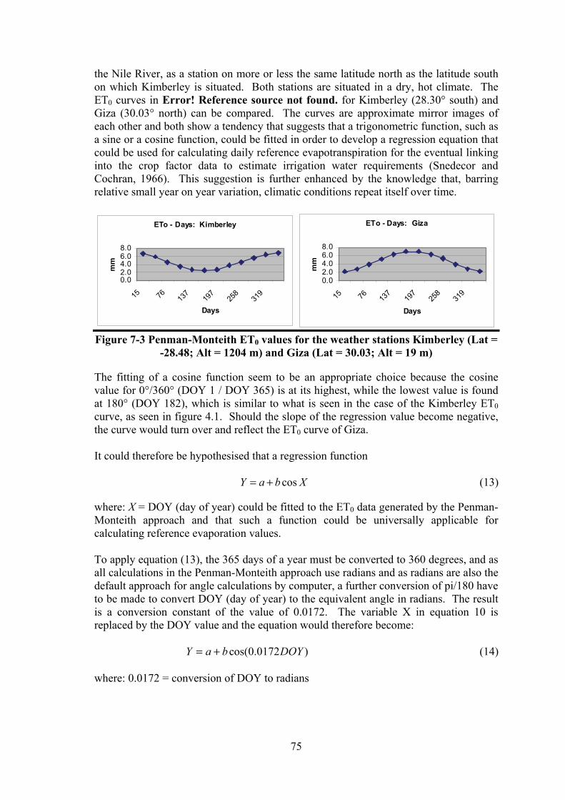
75
the Nile River, as a station on more or less the same latitude north as the latitude south on which Kimberley is situated. Both stations are situated in a dry, hot climate. The ET0 curves in Error! Reference source not found. for Kimberley (28.30° south) and Giza (30.03° north) can be compared. The curves are approximate mirror images of each other and both show a tendency that suggests that a trigonometric function, such as a sine or a cosine function, could be fitted in order to develop a regression equation that could be used for calculating daily reference evapotranspiration for the eventual linking into the crop factor data to estimate irrigation water requirements (Snedecor and Cochran, 1966). This suggestion is further enhanced by the knowledge that, barring relative small year on year variation, climatic conditions repeat itself over time.
ETo - Days: Kimberley
0.02.04.06.08.0
15 76 137
197
258
319
Days
mm
ETo - Days: Giza
0.02.04.06.08.0
15 76 137
197
258
319
Daysm
m
Figure 7-3 Penman-Monteith ET0 values for the weather stations Kimberley (Lat =
-28.48; Alt = 1204 m) and Giza (Lat = 30.03; Alt = 19 m)
The fitting of a cosine function seem to be an appropriate choice because the cosine value for 0°/360° (DOY 1 / DOY 365) is at its highest, while the lowest value is found at 180° (DOY 182), which is similar to what is seen in the case of the Kimberley ET0 curve, as seen in figure 4.1. Should the slope of the regression value become negative, the curve would turn over and reflect the ET0 curve of Giza. It could therefore be hypothesised that a regression function cosY a b X (13)
where: X = DOY (day of year) could be fitted to the ET0 data generated by the Penman-Monteith approach and that such a function could be universally applicable for calculating reference evaporation values. To apply equation (13), the 365 days of a year must be converted to 360 degrees, and as all calculations in the Penman-Monteith approach use radians and as radians are also the default approach for angle calculations by computer, a further conversion of pi/180 have to be made to convert DOY (day of year) to the equivalent angle in radians. The result is a conversion constant of the value of 0.0172. The variable X in equation 10 is replaced by the DOY value and the equation would therefore become: cos(0.0172 )Y a b DOY (14)
where: 0.0172 = conversion of DOY to radians
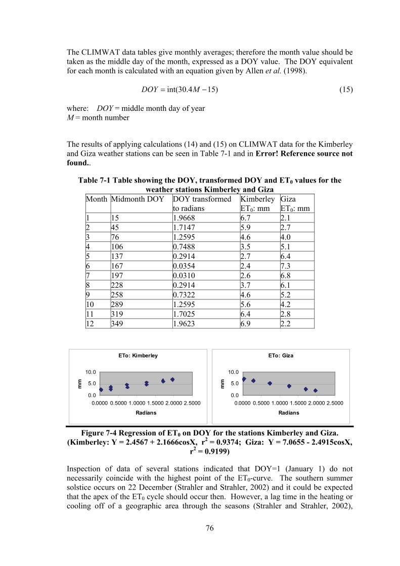
76
The CLIMWAT data tables give monthly averages; therefore the month value should be taken as the middle day of the month, expressed as a DOY value. The DOY equivalent for each month is calculated with an equation given by Allen et al. (1998). int(30.4 15)DOY M (15)
where: DOY = middle month day of year M = month number
The results of applying calculations (14) and (15) on CLIMWAT data for the Kimberley and Giza weather stations can be seen in Table 7-1 and in Error! Reference source not found..
Table 7-1 Table showing the DOY, transformed DOY and ET0 values for the weather stations Kimberley and Giza
Month Midmonth DOY DOY transformed to radians
Kimberley ET0: mm
Giza ET0: mm
1 15 1.9668 6.7 2.1 2 45 1.7147 5.9 2.7 3 76 1.2595 4.6 4.0 4 106 0.7488 3.5 5.1 5 137 0.2914 2.7 6.4 6 167 0.0354 2.4 7.3 7 197 0.0310 2.6 6.8 8 228 0.2914 3.7 6.1 9 258 0.7322 4.6 5.2 10 289 1.2595 5.6 4.2 11 319 1.7025 6.4 2.8 12 349 1.9623 6.9 2.2
ETo: Kimberley
0.0
5.0
10.0
0.0000 0.5000 1.0000 1.5000 2.0000 2.5000
Radians
mm
ETo: Giza
0.0
5.0
10.0
0.0000 0.5000 1.0000 1.5000 2.0000 2.5000
Radians
mm
Figure 7-4 Regression of ET0 on DOY for the stations Kimberley and Giza.
(Kimberley: Y = 2.4567 + 2.1666cosX, r2 = 0.9374; Giza: Y = 7.0655 - 2.4915cosX, r2 = 0.9199)
Inspection of data of several stations indicated that DOY=1 (January 1) do not necessarily coincide with the highest point of the ET0-curve. The southern summer solstice occurs on 22 December (Strahler and Strahler, 2002) and it could be expected that the apex of the ET0 cycle should occur then. However, a lag time in the heating or cooling off of a geographic area through the seasons (Strahler and Strahler, 2002),
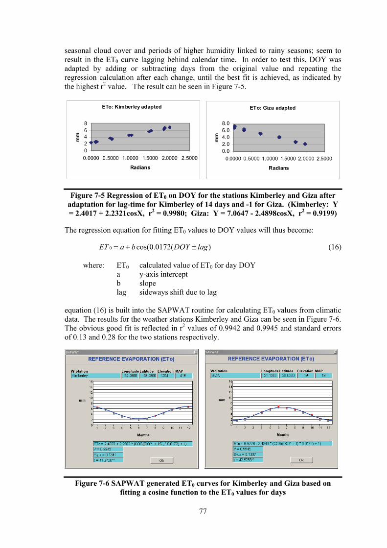
77
seasonal cloud cover and periods of higher humidity linked to rainy seasons; seem to result in the ET0 curve lagging behind calendar time. In order to test this, DOY was adapted by adding or subtracting days from the original value and repeating the regression calculation after each change, until the best fit is achieved, as indicated by the highest r2 value. The result can be seen in Figure 7-5.
ETo: Kimberley adapted
02468
0.0000 0.5000 1.0000 1.5000 2.0000 2.5000
Radians
mm
ETo: Giza adapted
0.02.04.06.08.0
0.0000 0.5000 1.0000 1.5000 2.0000 2.5000
Radians
mm
Figure 7-5 Regression of ET0 on DOY for the stations Kimberley and Giza after adaptation for lag-time for Kimberley of 14 days and -1 for Giza. (Kimberley: Y = 2.4017 + 2.2321cosX, r2 = 0.9980; Giza: Y = 7.0647 - 2.4898cosX, r2 = 0.9199)
The regression equation for fitting ET0 values to DOY values will thus become:
0 cos(0.0172( )ET a b DOY lag (16)
where: ET0 calculated value of ET0 for day DOY a y-axis intercept b slope lag sideways shift due to lag
equation (16) is built into the SAPWAT routine for calculating ET0 values from climatic data. The results for the weather stations Kimberley and Giza can be seen in Figure 7-6. The obvious good fit is reflected in r2 values of 0.9942 and 0.9945 and standard errors of 0.13 and 0.28 for the two stations respectively.
Figure 7-6 SAPWAT generated ET0 curves for Kimberley and Giza based on fitting a cosine function to the ET0 values for days

78
The application of equation (16) was tested on several other stations out of different climatic regions to verify that the results are that which are to be expected. The results can be seen in Figure 7-7.
Figure 7-7 The results of applying regression equation (16) on weather stations from a variety of climatic regions
The fit of the regression curves to calculated ET0 data as can be seen in Figure 7-7 seems good.
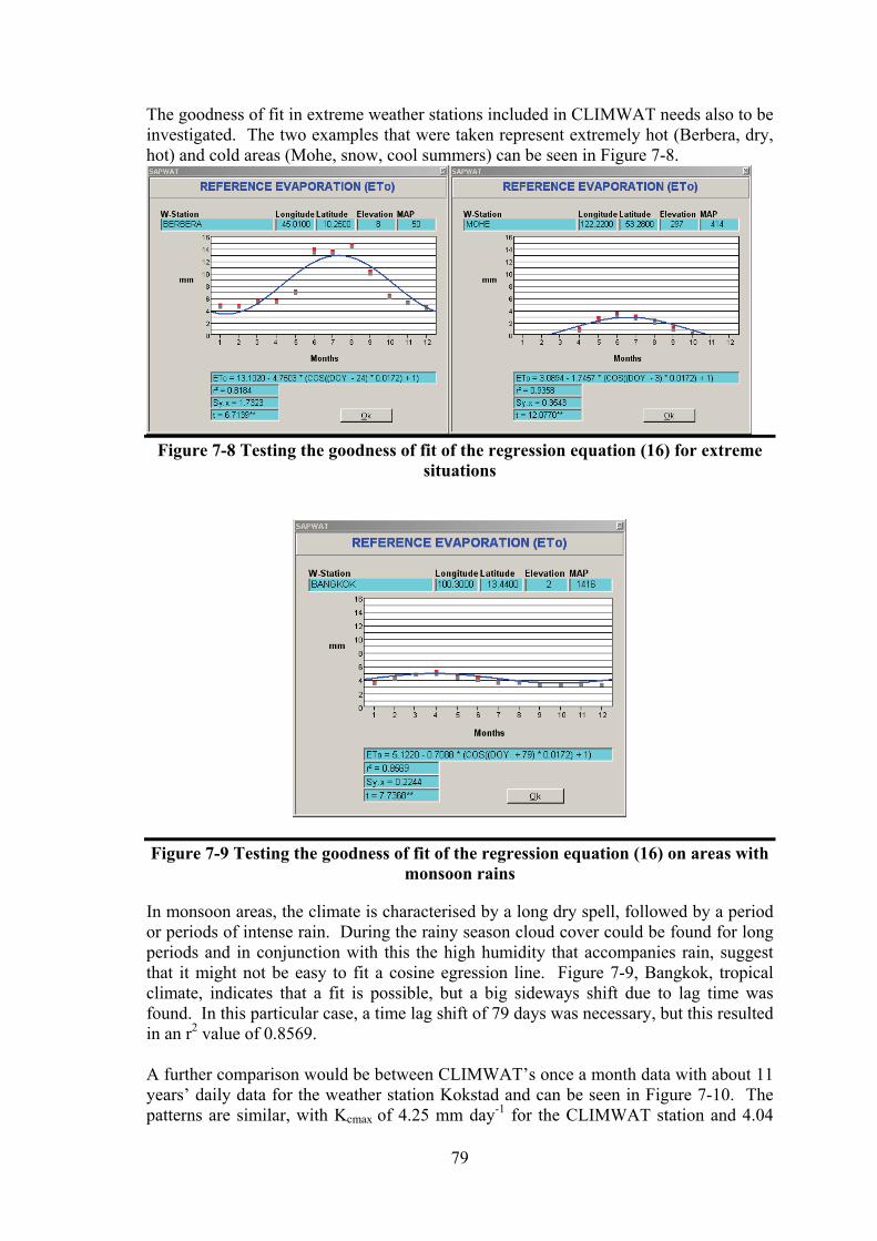
79
The goodness of fit in extreme weather stations included in CLIMWAT needs also to be investigated. The two examples that were taken represent extremely hot (Berbera, dry, hot) and cold areas (Mohe, snow, cool summers) can be seen in Figure 7-8.
Figure 7-8 Testing the goodness of fit of the regression equation (16) for extreme
situations
Figure 7-9 Testing the goodness of fit of the regression equation (16) on areas with monsoon rains
In monsoon areas, the climate is characterised by a long dry spell, followed by a period or periods of intense rain. During the rainy season cloud cover could be found for long periods and in conjunction with this the high humidity that accompanies rain, suggest that it might not be easy to fit a cosine egression line. Figure 7-9, Bangkok, tropical climate, indicates that a fit is possible, but a big sideways shift due to lag time was found. In this particular case, a time lag shift of 79 days was necessary, but this resulted in an r2 value of 0.8569. A further comparison would be between CLIMWAT’s once a month data with about 11 years’ daily data for the weather station Kokstad and can be seen in Figure 7-10. The patterns are similar, with Kcmax of 4.25 mm day-1 for the CLIMWAT station and 4.04

80
mm day-1 for the manual station. The more data included in the manual station data forces the Kcmin for the manual station to 0.8 mm day-1, which seems substantially lower than the 1.7 mm day-1 for the CLIMWAT station. As this lower value also coincides with the period of low growth and therefore low water use, the effect of the difference become much less than it would have been had this difference been found in midsummer when growth rate and water use would be at its peak.
Figure 7-10 A comparison of CLIMWAT and manual station with 11 years’ data for the weather station Kokstad
The overall impression of these results suggest that a trigonometric function (cosine) could be fitted successfully on the ET0 data for a station to generate a regression curve that could be used in conjunction of crop characteristic data for the calculation of irrigation water requirements.
7.5 Application in SAPWAT3
7.5.1 The SAPWAT3 ET0 calculator
This free-standing ET0 calculator uses weather data to calculate ET0 for each record in a weather station data table. When weather data is added to SAPWAT3, the program runs sequentially through all the records and does the necessary calculations to determine and store values for use in the calculation of the Penman-Monteith equation. This action includes the fitting of a regression curve to the data which enables SAPWAT3 to do time series irrigation requirement estimates for sub-periods of the total time series.
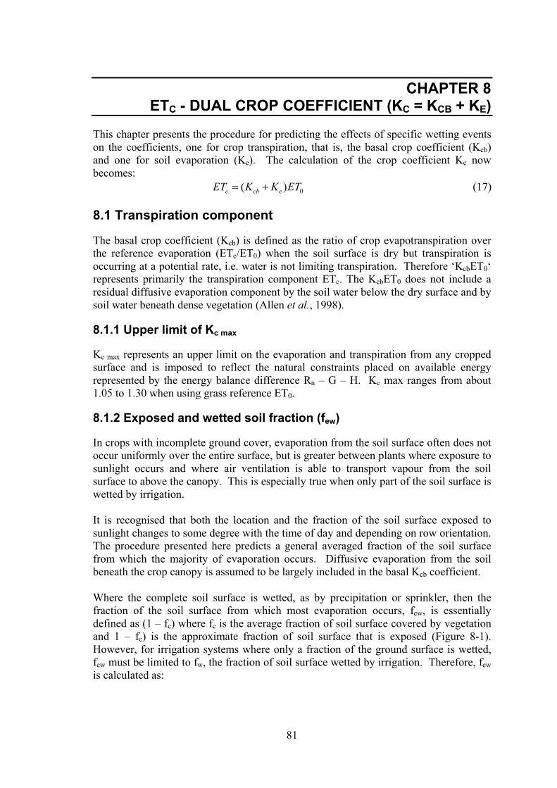
81
CHAPTER 8 ETC - DUAL CROP COEFFICIENT (KC = KCB + KE)
This chapter presents the procedure for predicting the effects of specific wetting events on the coefficients, one for crop transpiration, that is, the basal crop coefficient (Kcb) and one for soil evaporation (Ke). The calculation of the crop coefficient Kc now becomes: 0( )c cb eET K K ET (17)
8.1 Transpiration component
The basal crop coefficient (Kcb) is defined as the ratio of crop evapotranspiration over the reference evaporation (ETc/ET0) when the soil surface is dry but transpiration is occurring at a potential rate, i.e. water is not limiting transpiration. Therefore ‘KcbET0‘ represents primarily the transpiration component ETc. The KcbET0 does not include a residual diffusive evaporation component by the soil water below the dry surface and by soil water beneath dense vegetation (Allen et al., 1998).
8.1.1 Upper limit of Kc max
Kc max represents an upper limit on the evaporation and transpiration from any cropped surface and is imposed to reflect the natural constraints placed on available energy represented by the energy balance difference Rn – G – H. Kc max ranges from about 1.05 to 1.30 when using grass reference ET0.
8.1.2 Exposed and wetted soil fraction (few)
In crops with incomplete ground cover, evaporation from the soil surface often does not occur uniformly over the entire surface, but is greater between plants where exposure to sunlight occurs and where air ventilation is able to transport vapour from the soil surface to above the canopy. This is especially true when only part of the soil surface is wetted by irrigation. It is recognised that both the location and the fraction of the soil surface exposed to sunlight changes to some degree with the time of day and depending on row orientation. The procedure presented here predicts a general averaged fraction of the soil surface from which the majority of evaporation occurs. Diffusive evaporation from the soil beneath the crop canopy is assumed to be largely included in the basal Kcb coefficient. Where the complete soil surface is wetted, as by precipitation or sprinkler, then the fraction of the soil surface from which most evaporation occurs, few, is essentially defined as (1 – fc) where fc is the average fraction of soil surface covered by vegetation and 1 – fc) is the approximate fraction of soil surface that is exposed (Figure 8-1). However, for irrigation systems where only a fraction of the ground surface is wetted, few must be limited to fw, the fraction of soil surface wetted by irrigation. Therefore, few is calculated as:

82
min(1 , )ew c wf f f (18)
Where: 1 – fc Average exposed soil fraction not covered (or shadowed) by vegetation [0.01-1]
fw Average fraction of soil surface wetted by irrigation or precipitation [0.01-1]
The limitation imposed by equation (18) assumes that the fraction of soil wetted by irrigation occurs within the fraction of soil exposed to sunlight and ventilation. Drip irrigation might be the exception because in most cases the wetted area is under the crop canopy. In this case, it may be necessary to reduce the values to about one-half or one-third of the shown value (Allen et al., 1998).

83
Figure 8-1 Determination of variable few (cross-hatchet areas) as a function of
ground surface coverage (fc) and the fraction of the surface wetted (fw) (Allen et al., 1998).
8.1.3 Fraction of soil surface wetted by irrigation or precipitation
Table 8-1 presents typical values for fw. Where a mixture of irrigation and precipitation occur within the same drying period or the same day, the value of fw should be based on a weighted average of the fw for precipitation (fw = 1) and the fw of the irrigation system. The weighting should be approximately proportional to the infiltration from each water source (Allen et al., 1998).

84
Table 8-1 Common values of fraction of soil surface wetted by irrigation or precipitation (Allen et al., 1998)
Wetting event fw Precipitation Sprinkler irrigation Basin irrigation Border irrigation Furrow irrigation (every furrow), narrow bedFurrow irrigation (every furrow), wide bed Furrow irrigation (alternated rows) Trickle irrigation
1.0 1.0 1.0 1.0 0.6-1.0 0.4-0.6 0.3-0.5 0.3-0.4
.
8.1.3.1 Exposed soil surface (1 – fc)
The fraction of soil surface that is covered by vegetation is termed fc. Therefore, (1 – fc) represents the fraction of the soil that is exposed to sunlight and air ventilation and which serve as the site for the majority of evaporation from the wet soil. The value for fc is limited to <0.99. The user should assume appropriate values for the various growth stages. Typical values for fc and (1 – fc) are given in Table 8-2.
Table 8-2 Common values of fractions covered by vegetation (fc) and exposed sunlight (1 – fc) (Allen et al., 1998)
Crop growth stage fc 1 – fc Initial stage Crop development stageMid-season stage Late season stage
0.0-0.10.1-0.80.8-1.00.8-0.2
1.0-0.90.9-0.20.2-0.00.2-0.8
Application of equation (18) predicts that fc decreases during the late season period in proportion to Kcb, even though the ground cover may remain covered with senescing vegetation. This prediction helps to account for the local transport of sensible heat from senescing leaves to the soil surface below (Allen et al., 1998).
8.2 Daily calculation of Ke
The estimation of Ke in the calculation period requires a daily water balance computation for the surface soil layer for the calculation of the cumulative evaporation or depletion for the wet condition. The daily soil water balance equation for the exposed and wetted soil fraction few is seen in Figure 8-2:
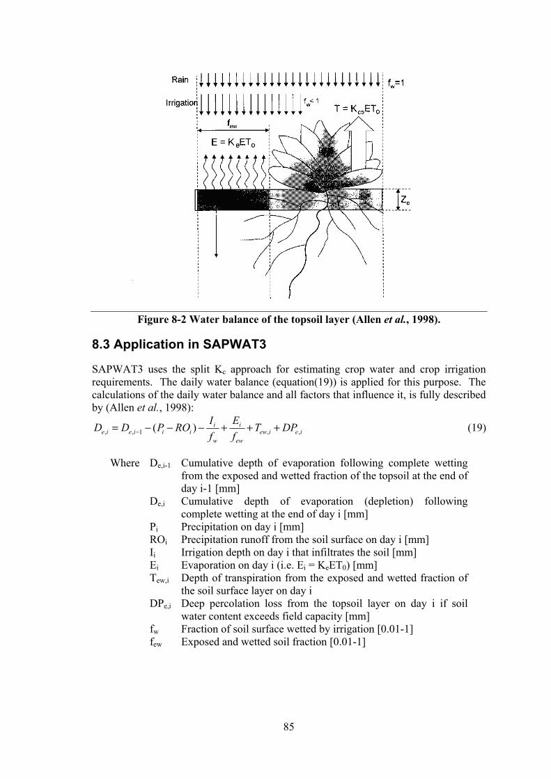
85
Figure 8-2 Water balance of the topsoil layer (Allen et al., 1998).
8.3 Application in SAPWAT3
SAPWAT3 uses the split Kc approach for estimating crop water and crop irrigation requirements. The daily water balance (equation(19)) is applied for this purpose. The calculations of the daily water balance and all factors that influence it, is fully described by (Allen et al., 1998):
, , 1 , ,( ) i ie i e i i i ew i e i
w ew
I ED D P RO T DP
f f (19)
Where De,i-1 Cumulative depth of evaporation following complete wetting from the exposed and wetted fraction of the topsoil at the end of day i-1 [mm]
De,i Cumulative depth of evaporation (depletion) following complete wetting at the end of day i [mm]
Pi Precipitation on day i [mm] ROi Precipitation runoff from the soil surface on day i [mm] Ii Irrigation depth on day i that infiltrates the soil [mm] Ei Evaporation on day i (i.e. Ei = KeET0) [mm] Tew,i Depth of transpiration from the exposed and wetted fraction of
the soil surface layer on day i DPe,i Deep percolation loss from the topsoil layer on day i if soil
water content exceeds field capacity [mm] fw Fraction of soil surface wetted by irrigation [0.01-1] few Exposed and wetted soil fraction [0.01-1]
86
CHAPTER 9 ETC UNDER SOIL WATER STRESS CONDITIONS
Forces acting on the soil water can decrease its potential energy and make it less available for plant root extraction. When the soil is wet, the water has a high potential energy, is released relatively free to move and is easily taken up by the plant roots. In dry soils, the water has a low potential energy and is strongly bound by capillary and adsorptive forces to the soil matrix, and is less easily extracted by the crop. When the potential energy of the soil water drops below a threshold value, the crop is said to be water stressed. The effects of soil water stress are described by multiplying the basal crop coefficient by a water stress coefficient Ks (Allen et al., 1998).
9.1 Soil water availability
9.1.1 Total available water (TAW)
Soil water availability refers to the capacity of a soil to retain water available to plants. After heavy rain or irrigation, the soil will drain until field capacity is reached. Field capacity is the amount of water that a well-drained soil should hold against gravitational forces, or the amount of water remaining when the downward drainage has markedly decreased. In the absence of water supply, the water content in the root zone decreases as a result of water uptake by the crop. As water uptake progresses, the remaining water is held to the soil particles with greater force, lowering its potential energy and making it more difficult for the plants to extract it. Eventually a point is reached where the crop can no longer extract the remaining water. The water uptake becomes zero when wilting point is reached. Wilting point is the water content at which plants will permanently wilt (Allen et al., 1998). As the water content above field capacity cannot be held against the forces of gravity and will drain and as the water content below wilting point cannot be extracted by plant roots, the total available water in the root zone is the difference between the water content at field capacity and wilting point (Allen et al., 1998). 1000( )FC WP rTAW Z (20)
Where TAW The total available water in the root zone [mm] θFC The water content at field capacity [m3 m-3] θWP The water content at wilting point [m3 m-3] Zr The rooting depth [m]
TAW is the amount of water that a crop can extract from its root zone and its magnitude depends on the type of soil and the rooting depth.
9.1.2 Readily available water (RAW)
Although water is theoretically available until wilting point, crop water uptake is reduced well before wilting point is reached. Where the soil is sufficiently wet, the soil supplies water fast enough to meet the atmospheric demand of the crop, and water uptake equals ETc. As the soil water content decreases, water becomes more strongly

87
bound to the soil matrix and is more difficult to extract. When the soil water content drops below a threshold value, soil water can no longer be transported quickly enough towards the root to respond to the transpiration demand and the crop begins to experience stress. The fraction of TAW that a crop can extract from the root zone without suffering water stress is the readily available soil water (Allen et al., 1998): RAW pTAW (21)
Where RAW The readily available soil water in the root zone [mm] P Average fraction of TAW that can be depleted from the
root zone before moisture stress (reduction in ET) occurs [0-1]
The value of p normally varies from 0.3 for shallow rooted plants at high rates of ETc (> 8 mm d-1) to 0.7 for deep rooted plants at low rates of ETc (< 3 mm d-1). A value for 0.5 for p is commonly used for many crops (Allen et al., 1998). The fraction p is a function of the evaporation power of the atmosphere. At low rates of ETc, the p values are higher than at high rates of ETc. At high rates of ETc, during hot dry weather, p is lower than usual and the soil can be relatively wet when stress starts to occur. When the crop evapotranspiration is low, p will be up to 20% more than expected values. A numerical approximation for adjusting for ETc rate is: 0.04(5 )table cp p ET (22)
Where ptable Tabulated values for p For 0.2 ≤ p ≤ 0.8
To express the tolerance of crops to water stress as a function of the fraction of the TAW is not wholly correct. The rate of root water uptake is in fact more directly influenced by the potential energy level of the soil water (soil matric potential and associated hydraulic conductivity) than by water content. As a certain soil matric potential corresponds in different soil types with different soil water contents, the value for p is also a function of the soil type. Generally, it can be stated that for fine texture soils (clay), the listed p values can be reduced by 5-10%, while for more coarse textured soils (sand), they can be increased by 5-10% (Allen et al., 1998).
9.2 Water stress coefficient (Ks)
The effects of soil water stress on crop ET are described by reducing the value for the crop coefficient. This is accomplished by multiplying the crop coefficient by the water stress coefficient (equation (23)). Water content in the root zone can also be expressed by root zone depletion, Dr, i.e. water shortage relative to field capacity. At field capacity, the root zone depletion is zero (Dr = 0). When soil water is extracted by evapotranspiration the depletion increases and stress will be induced when Dr becomes equal to RAW. After root zone depletion exceeds RAW, the water content drops to less than potential value and the crop evapotranspiration begins to decrease in proportion to the amount of water remaining in the root zone, as shown in Figure 9-1.
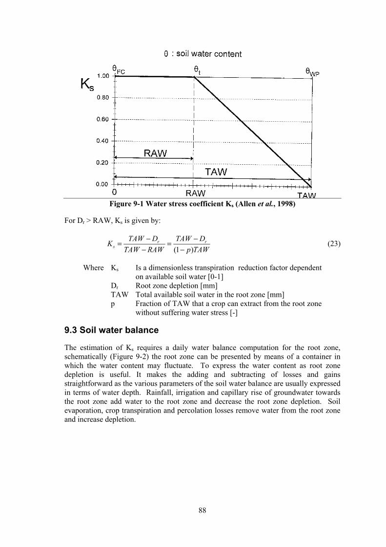
88
Figure 9-1 Water stress coefficient Ks (Allen et al., 1998)
For Dr > RAW, Ks is given by:
(1 )
r rs
TAW D TAW DK
TAW RAW p TAW
(23)
Where Ks Is a dimensionless transpiration reduction factor dependent on available soil water [0-1]
Dr Root zone depletion [mm] TAW Total available soil water in the root zone [mm] p Fraction of TAW that a crop can extract from the root zone
without suffering water stress [-]
9.3 Soil water balance
The estimation of Ks requires a daily water balance computation for the root zone, schematically (Figure 9-2) the root zone can be presented by means of a container in which the water content may fluctuate. To express the water content as root zone depletion is useful. It makes the adding and subtracting of losses and gains straightforward as the various parameters of the soil water balance are usually expressed in terms of water depth. Rainfall, irrigation and capillary rise of groundwater towards the root zone add water to the root zone and decrease the root zone depletion. Soil evaporation, crop transpiration and percolation losses remove water from the root zone and increase depletion.

89
Figure 9-2 Water balance of the root zone (Allen et al., 1998).
The daily water balance, expressed in terms of depletion at the end of the day is: , , 1 ,( )r i r i i i i c i iD D P RO I CR ET DP (24)
Where Dr,i Root zone depletion at end of day i [mm] Dr,i-1 Water content in the root zone at the end of the previous
day, i-1 [mm] Pi Precipitation on day i [mm] ROi Runoff from the soil surface on day i [mm] Ii Net irrigation depth on day i that infiltrates the soil [mm] CRi Capillary rise from the groundwater table on day i [mm] ETc,i Crop evapotranspiration on day i [mm] DPi Water loss out of the root zone by deep percolation on day
i [mm]
9.3.1 Limits on Dr,i
In Figure 9-2 it is assumed that water can be stored in the root zone until field capacity is reached. Following heavy rain or irrigation, the water content might temporarily exceed field capacity. The total amount of water above field capacity is assumed to be lost the same day by deep percolation following any ET for that day. By assuming that the root zone is at field capacity following heavy rain or irrigation, the minimum value for depletion Dr,i is zero. As a result of percolation and evapotranspiration, the water content in the root zone will gradually decrease and the root zone depletion will increase. In the absence of any wetting event, the water content will steadily reach the minimum value θWP. At that moment no water is left for evapotranspiration in the root

90
zone, Ks become zero, and the root zone depletion has reached its maximum value TAW.
9.3.2 Initial depletion
The initial depletion Dr,r-1 should be estimated. The initial depletion can be derived from the measured soil water content by: , 1 11000( )r i FC i rD Z (25)
Where θi-1 is the average soil water content for the effective root zone. Following heavy rain or irrigation, the user can assume that the root zone is near field capacity, i.e. Dr,i-1 ≈ 0.
9.3.3 Precipitation (P), runoff (RO) and irrigation (I)
Pi is equivalent to daily precipitation. Daily precipitation in amounts less than about 0.2ET0 is normally entirely evaporated and can usually be ignored in the water balance calculations. Ii is equivalent to the mean infiltrated irrigation depth expressed for the entire field surface. Runoff from the surface during precipitation can be predicted using standard procedures from hydrological text.
9.3.4 Capillary rise (CR)
The amount of water transported upwards by capillary rise from the water table to the root zone depends on the soil type, the depth of the water table and the wetness of the root zone. CR can normally be assumed to be zero when the water table is more than about 1 m below the bottom of the root zone.
9.3.5 Evapotranspiration
Where the soil water depletion is smaller than RAW, the crop evapotranspiration equals ETc = KcET0. As soon as Dr,i exceeds RAW, the crop evapotranspiration is reduced and ETc can be computed by incorporating equation (23).
9.3.6 Deep percolation
Following heavy rain or irrigation, the soil water content in the root zone might exceed field capacity. In this simple procedure it is assumed that the soil water content as at θFC within the same day of the wetting event, so that the depletion Dr,i in equation (25) becomes zero. Therefore, following a heavy rain or irrigation: , , 1( )i i i c i r iDP P RO I ET D (26)
As long as the soil water content in the root zone is below field capacity (i.e. Dr,i >0), the soil will not drain and DPi = 0 (Allen et al., 1998).

91
9.4 Forecasting or allocating irrigations
Irrigation is required when rainfall is insufficient for the water lost by evapotranspiration. The primary objective of irrigation is to apply water at the right period and in the right amount. By calculating the soil water balance on the root zone on a daily basis (equation (24)), the timing and the depth of irrigations can be planned. To avoid crop water stress, irrigation should be applied before or at the moment when the readily available soil water is depleted (Dr,i ≤ RAW). To avoid deep percolation losses that may leach relevant nutrients out of the root zone, the net irrigation depth should be smaller than or equal to the root zone depletion (Ii ≤ Dr,i).
9.5 Effects of soil salinity
Salts in the soil water solution can reduce evapotranspiration by making water less available for the plant root extraction. Salts have an affinity for water and hence additional force is required for the crop to extract water from a saline soil. The presence of salts in the soil water solution reduces the total potential energy of the soil water solution. In addition, some salts cause toxic effects in plants and can reduce plant metabolism and growth. A function is included in SAPWAT3 that predicts the reduction in evapotranspiration caused by salinity of soil water. There is evidence that crop yield and transpiration are not as sensitive to low osmotic potential as they are to low matric potential. Under saline conditions, many plants are able to partially compensate for low osmotic potential of the soil water by building up higher internal solute contents. This is done by absorbing ions from the soil solution and by synthesizing organic osmolytes. Both of these reactions reduce the impact of osmotic potential on water availability. However, synthesis of organic osmolytes does require expenditure of metabolic energy. Therefore plant growth is often reduced under saline conditions. The reduced plant growth impacts on transpiration by reducing ground cover and sometimes partial stomatal closure. Other impacts of salts in the soil include direct sodium and chloride toxicities and induced nutrient deficiencies. These deficiencies reduce plant growth by reducing the rate of leaf elongation, the enlargement, and the division of cells in leaves. The modality depends on the method of irrigation. With sprinkler irrigation, adsorption of sodium and chloride through the leaf can result in toxic conditions for all crop species. With surface or trickle irrigation, direct toxic conditions generally occur only in vine and tree crops; however, high levels of sodium can induce calcium deficiencies for all crop species. Since salt concentration changes as the soil water content changes, soil salinity is normally measured and expressed on the basis of the electrical conductivity of the saturation extract of the soil (ECe). The ECe is defined as the electrical conductivity of the soil water solution after the addition of a sufficient quantity of distilled water to bring the soil water content to saturation. ECe is typically expressed in milliSiemens per meter (mS m-1). Under optimum management conditions, crop yields remain at potential levels until a specific threshold electrical conductivity of the saturation soil water extract (ECe threshold) is reached. If the average ECe of the root zone increases above this critical threshold value, the yield is presumed to begin to decrease linearly in proportion to the increase in salinity. The rate of decrease in yield with increase in salinity is
92
usually expressed as a slope, b, having units of % reduction in yield per mS/m increase in ECe. Not all plants respond to salinity in a similar manner; some crops can produce acceptable yields at much higher soil salinity levels than others. This is because some crops are more able to make the needed osmotic adjustments that enable them to extract more water from a saline soil, or they may be more tolerant of some of the toxic effects of saline water. The effect of soil salinity on yield and crop evapotranspiration is crop specific. The ECe threshold and b parameters were determined primarily in research experiments using nearly steady-state irrigation where soil water contents were maintained at levels close to field capacity. However, under most types of irrigation scheduling for sprinkler and surface irrigation, the soil water content is typically depleted to well below field capacity, so that the EC of the soil water solution, ECSW, increases prior to irrigation, even though the EC of the saturation extract does not change. The increased salt concentration in the soil water solution reduces the osmotic potential of the soil water solution (it becomes more negative), so that the plant must expend more metabolic energy and may exert more mechanical force to absorb water. In addition, metabolic and toxic effects of salts on plants may become more pronounced as the soil dries and concentrations increase. However, the variation in soil water content during an irrigation interval has not been found to strongly influence crop evapotranspiration. This is because of the rise of soil water content to levels that are above that experienced under steady state irrigation early in a long irrigation interval. There is a similar, counteractive decrease in soil water content later in a long irrigation interval. In addition, the distribution of salts in the root zone under low frequency irrigation can reduce salinity impacts during the first portion of the irrigation interval. Also, under high frequency irrigation of the soil surface, soil evaporation losses are higher. Consequently, given the same application depth, the leaching fraction is reduced. For these reasons, the length of irrigation interval and the change in EC of soil water during the interval have usually not been found to be factors in the reduction of ET, given that the same depths of water are infiltrated into the root zone over time. Research has found that effects of soil salinity and water stress are generally additive in their impacts on crop evapotranspiration. Therefore, the same yield-ET functions may hold for both water shortage induced stress and for salinity induced stress water (Allen et al., 1998).
9.6 Yield-salinity relationship
A widely practiced approach for predicting the reduction in crop yield due to salinity presumes that, under optimum management conditions, crop yields remain at potential levels until a specific threshold electrical conductivity of the soil water solution is reached. When salinity increases beyond this threshold, crop yields are presumed to decrease linearly in proportion to the increase in salinity. The soil water salinity is expressed as the electrical conductivity of the saturation extract, ECe. In equation form, the procedure is:

93
1 ( )100
ae e threshold
m
Y bEC EC
Y (27)
Where Ya Actual crop yield Ym maximum expected crop yield when ECe < ECe threshold ECe mean electrical conductivity of the saturation extract for
the root zone [dS m-1] ECe threshold electrical conductivity of the saturation extract at the
threshold of ECe when crop yield first reduces below Ym [dS m-1]
b reduction in yield per increase in ECe [%/(dS m-1)] where ECe > ECe threshold
9.7 Yield-moisture stress relationship
A simple, linear crop-water production function was introduced in the FAO Irrigation and Drainage Paper No. 33 (Doorenbos et al., 1986) to predict the reduction in crop yield when crop stress was caused by a shortage of soil water:
1 1 c adja
ym c
ETYK
Y ET
(28)
Where Ky a yield response factor [-] ETc adj adjusted (actual) crop evapotranspiration [mm d-1] ETc crop evapotranspiration for standard conditions (no
water stress) [mm d-1] Ky is a factor that describes the reduction in relative yield according to the reduction in ETc caused by soil water shortage. In FAO No. 33, Ky values are crop specific and may vary over the growing season. In general, the decrease in yield due to water deficit during the vegetative and ripening period is relatively small, while during the flowering and yield formation periods it will be large. Values for Ky for individual growth periods and for the complete growing season have been included in the FAO Irrigation and Drainage Paper No. 33.

94
Figure 9-3 The effect of soil salinity on the water stress coefficient (Allen et al.,
1998)
9.7.1 Limitations
Because the impact of salinity on plant growth and yield and on crop evapotranspiration is a time-integrated process, generally only the seasonal value for Ky is used to predict reduction in evapotranspiration. For crops where Ky is unknown, the user may use Ky = 1 in equations (27) and (28) or may select the Ky for a crop type that has similar behaviour. equations (27) and (28) are suggested as only approximate estimates of salinity impacts on ET, and represent general effects of salinity on evapotranspiration as occurring over an extended period of time (as measured in weeks or months). These equations are not expected to be accurate for predicting ETc for specific days. Nor do they include other complicating effects such as specific ion toxicity. Application of equations (27) and (28) presumes that the ECe represents the average ECe for the root zone. The equations presented may not be valid at high salinity, where the linear relationships between ECe, crop yield and Ks may not hold. The use of equations (27) and (28) should usually be restricted to ECe < ECthreshold + 50/b. In addition, the equations predict Ya = 0 before Ks = 0 when Ky > 1 and vice versa. As indicated earlier, reduction in ETc in the presence of soil salinity is often partially caused by reduced plant size and fraction of ground cover. These effects are largely included in the coefficient values in table 23 in (Allen et al., 1998). Therefore, where plant growth is affected by salinity and equations (27) and (28) are applied, no other reductions in Kc are required, for example using LAI or fraction of ground cover.
9.7.2 Application
Under steady state conditions, the value for ECe can be predicted as a function of EC of the irrigation water (ECiw) and the leaching fraction, using a standard leaching formula. For example, the FAO-29 leaching formula LR = ECiw / (5 ECe – ECiw) predicts the
95
leaching requirement when approximately a 40-30-20-10 percent water extraction occurs from the upper to the lower quarters of the root zone prior to irrigation. ECiw is the electrical conductivity of the irrigation water. From this equation, ECe is estimated as:
1
5iw
e
ECLFEC
LF
(29)
Where LF, the actual leaching fraction, is used in place of LR, the leaching requirement. Equation (29) predicts ECe = 1.5 ECiw under conditions where a 15-20 percent leaching fraction is employed. Other leaching fraction equations can be used in place of the FAO-29 equation to fit local characteristics. Equation (29) is only true if the irrigation water quality and the leaching fraction are constant over the growing season. Time is required to attain a salt equilibrium in the soil. If there are important winter rains of high quality water and often excellent leaching, the salt balance in the soil will be different at the beginning of the season and with a lower average ECe of the root zone than would be predicted from equation (29). An appropriate local calibration of equation (29) is desirable under these particular conditions. Forces acting on the soil water decrease its potential energy and make it less available for plant root extraction. When the soil is wet, the water has a high potential energy, is released relatively free to move and is easily taken up by the plant roots. In dry soils, the water has a low potential energy and is strongly bound by capillary and adsorptive forces to the soil matrix, and is less easily extracted by the crop (Allen et al., 1998). When the potential energy of the soil water drops below a threshold value, the crop is said to be water stressed. The effects of soil water stress are described by multiplying the basal crop coefficient by the water stress coefficient Ks (Allen et al., 1998): 0( )cadj s cb eET K K K ET (30)
Ks describe the effect of water stress on crop transpiration. For soil water limiting conditions, Ks < 1. Where there is no soil water stress, Ks = 1 (Allen et al., 1998).

96
CHAPTER 10 IRRIGATION SYSTEMS
10.1 The irrigation system data table
Irrigation systems and their respective default efficiencies were hard coded into the previous version of SAPWAT. In SAPWAT3 this data is placed in a data table that is used as a lookup table by the program. This gives the user the ability to add, edit or delete data or to adapt values to suit local conditions. Table 10-1 shows the irrigation systems and their efficiencies as included in SAPWAT3.
Table 10-1 Irrigation systems and efficiencies included in SAPWAT3 System Application efficiency (%) Distribution uniformity (%)Centre pivot 80 100 Drip 95 100 Flood: basin 75 100 Flood: border 50 100 Flood: furrow 55 100 Linear 85 100 Micro spray 90 100 Micro sprinkler 85 100 Sprinkler: big gun 70 100 Sprinkler: boom 75 100 Sprinkler: dragline 75 100 Sprinkler: hop-along 75 100 Sprinkler: permanent 85 100 Sprinkler: quick-coupling 75 100 Sprinkler: side roll 75 100 Sprinkler: travelling boom 80 100 Sprinkler: travelling gun 75 100 Subsurface 95 100 Sprinkler: permanent (floppy) 85 100
In an unpublished report on Deliverable 3 of WRC Project K5/1482/4, “Standards and guidelines for improved efficiency of irrigation water use from dam wall release to root zone application”, the following definitions are given for application efficiency (AE) and for distribution uniformity (DU). The definition of DU changes slightly, depending on the irrigation system. The definitions given in this report are:
AE average depth of irrigation water contributing to target as a percentage of average depth of irrigation water applied.
DUlq average application of the lowest 25% as a percentage of the average application of the total system.
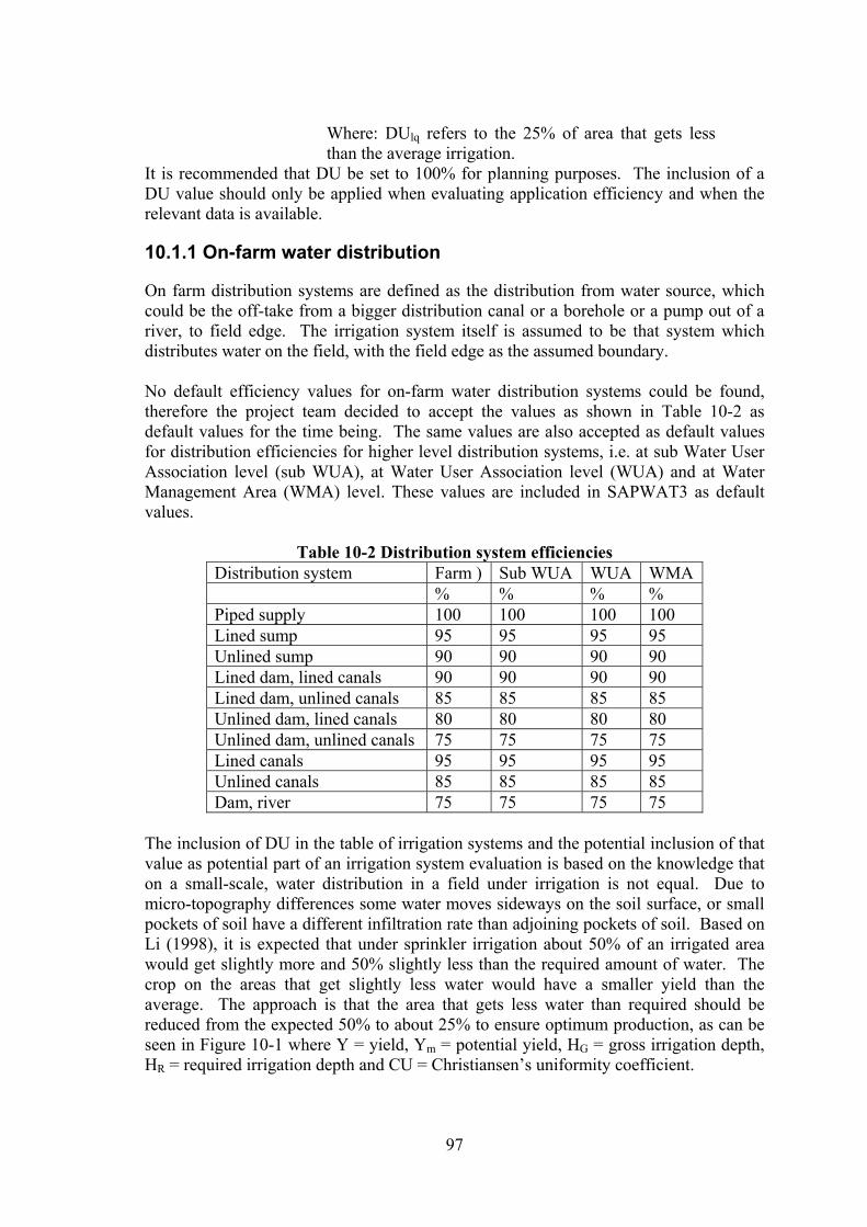
97
Where: DUlq refers to the 25% of area that gets less
than the average irrigation. It is recommended that DU be set to 100% for planning purposes. The inclusion of a DU value should only be applied when evaluating application efficiency and when the relevant data is available.
10.1.1 On-farm water distribution
On farm distribution systems are defined as the distribution from water source, which could be the off-take from a bigger distribution canal or a borehole or a pump out of a river, to field edge. The irrigation system itself is assumed to be that system which distributes water on the field, with the field edge as the assumed boundary. No default efficiency values for on-farm water distribution systems could be found, therefore the project team decided to accept the values as shown in Table 10-2 as default values for the time being. The same values are also accepted as default values for distribution efficiencies for higher level distribution systems, i.e. at sub Water User Association level (sub WUA), at Water User Association level (WUA) and at Water Management Area (WMA) level. These values are included in SAPWAT3 as default values.
Table 10-2 Distribution system efficiencies Distribution system Farm ) Sub WUA WUA WMA % % % % Piped supply 100 100 100 100 Lined sump 95 95 95 95 Unlined sump 90 90 90 90 Lined dam, lined canals 90 90 90 90 Lined dam, unlined canals 85 85 85 85 Unlined dam, lined canals 80 80 80 80 Unlined dam, unlined canals 75 75 75 75 Lined canals 95 95 95 95 Unlined canals 85 85 85 85 Dam, river 75 75 75 75
The inclusion of DU in the table of irrigation systems and the potential inclusion of that value as potential part of an irrigation system evaluation is based on the knowledge that on a small-scale, water distribution in a field under irrigation is not equal. Due to micro-topography differences some water moves sideways on the soil surface, or small pockets of soil have a different infiltration rate than adjoining pockets of soil. Based on Li (1998), it is expected that under sprinkler irrigation about 50% of an irrigated area would get slightly more and 50% slightly less than the required amount of water. The crop on the areas that get slightly less water would have a smaller yield than the average. The approach is that the area that gets less water than required should be reduced from the expected 50% to about 25% to ensure optimum production, as can be seen in Figure 10-1 where Y = yield, Ym = potential yield, HG = gross irrigation depth, HR = required irrigation depth and CU = Christiansen’s uniformity coefficient.
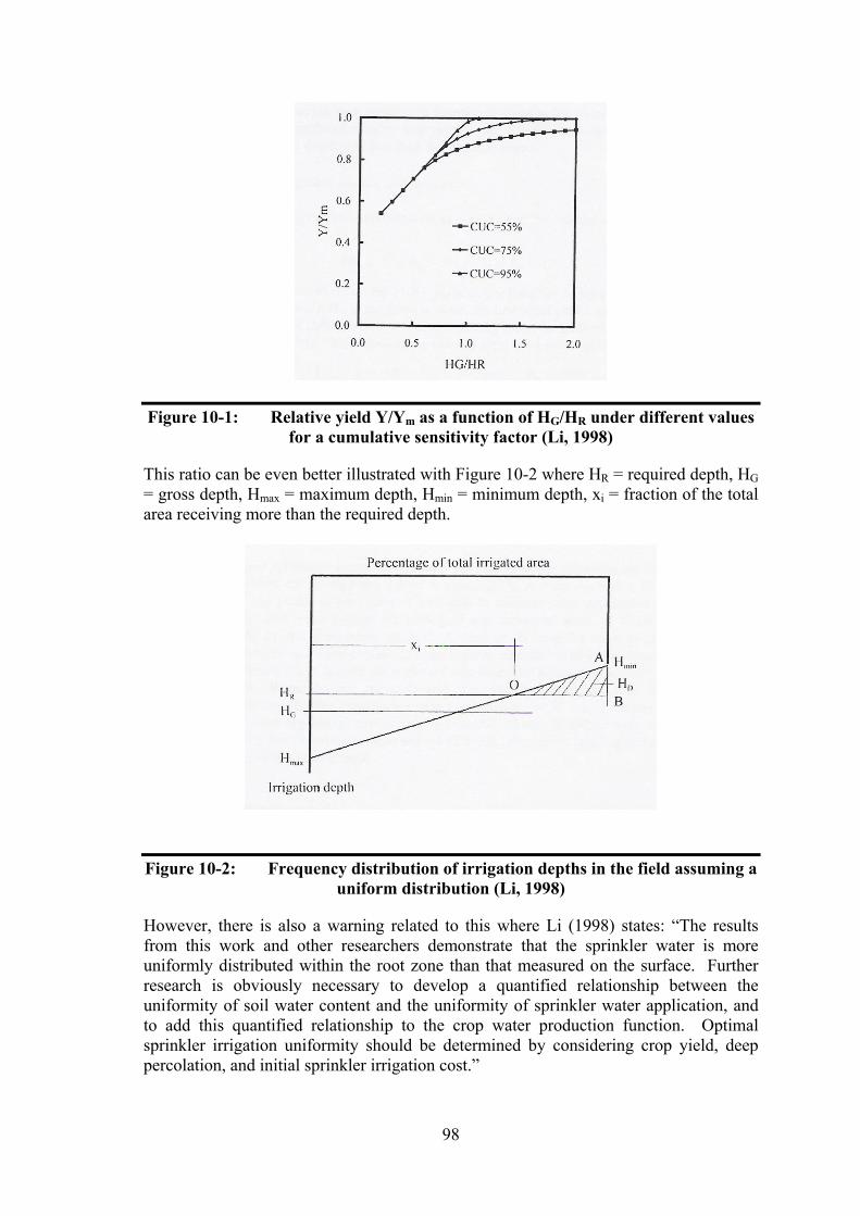
98
Figure 10-1: Relative yield Y/Ym as a function of HG/HR under different values for a cumulative sensitivity factor (Li, 1998)
This ratio can be even better illustrated with Figure 10-2 where HR = required depth, HG = gross depth, Hmax = maximum depth, Hmin = minimum depth, xi = fraction of the total area receiving more than the required depth.
Figure 10-2: Frequency distribution of irrigation depths in the field assuming a uniform distribution (Li, 1998)
However, there is also a warning related to this where Li (1998) states: “The results from this work and other researchers demonstrate that the sprinkler water is more uniformly distributed within the root zone than that measured on the surface. Further research is obviously necessary to develop a quantified relationship between the uniformity of soil water content and the uniformity of sprinkler water application, and to add this quantified relationship to the crop water production function. Optimal sprinkler irrigation uniformity should be determined by considering crop yield, deep percolation, and initial sprinkler irrigation cost.”
99
CHAPTER 11 ENTERPRISE BUDGETS
11.1 Introduction
The need for the inclusion of an economic analysis module in SAPWAT3 to enhance its capability as a planning tool, has been expressed by more and more users recently as the conviction grew amongst some of the users that planning irrigation water use without considering the economic impact, does not give enough of a picture to base future panning for crop production on. It was therefore decided to expand the capability of SAPWAT3 as a planning tool by including a COMBUD-type analyses calculator in the program. Inclusion of such a facility will be such that the user who does not want to do an economic analysis, would still be able to do the irrigation requirement calculation with the same ease to which he has become accustomed to in the present version of SAPWAT. The user, who wants to make use of this capability, can do the necessary analyses and store the results in the irrigation requirement table for future use. Three levels of data-input are provided for. At the lowest level provision is made for those users who only have a general idea of total income and expenditure. In this case the only required input is total expected income and total expected variable cost. The other end of the input-level is for those users who have a complete breakdown of every item of input. The middle level provide for an in-between situation, e.g. the user knows what his expected cost for fertiliser will be, but does not know what the cost of each of the fertiliser components will be. The introduction of enterprise budgets as part of the irrigation water requirement planning process, adds an alternative option that can influence decision-making. This facility, with the added function of calculating income per unit water, as well as the more usual income per unit land as efficiency measures, adds value to the irrigation water requirement planning. The irrigator can now build a picture of what the results of his decision would be, not only on total water use, but on his expected income as well. Enterprise budgets give a value as a point in time; they are not a continuous function that could predict cash-flow over time. However, they could be very good indicators for choosing profitable crops. It is unfortunately so that, in the past, the estimation of irrigation water requirement has been seen in isolation from the economic side. To counter this trend and to provide such a facility for the many users of SAPWAT who asked for it, SAPWAT3 now contains an enterprise budget module that is linked to the water requirement table. By changing input data, such as the area of a crop or irrigation strategies through a process of “what-iffing”, the user can now select not only the cropping system with an optimum potential water use, but can select an optimum combination of water use and gross margin for his situation. Incorporating gross margin calculations in SAPWAT3 may seem straightforward. However, some major changes to the previous version of SAPWAT are necessary to
100
provide an interactive planning model with gross margin calculations. The old version of SAPWAT only showed the results of one analysis at a time. Although the model provides the flexibility to change irrigation schedules and view the results quickly, no functionality was provided to save different scenarios and to compare these scenarios. Apart from irrigation timing and amounts of irrigation, irrigation planning typically involves the decisions on which crop to plant, how many hectares to plant, which soils to plant and which irrigation technology to use. Thus, irrigation planning is mainly concerned with reconciling resource availability with use, while trying to maximise profits. It is important to note that the newly developed SAPWAT3 is not an optimisation model. Rather it allows the user to explore the impact of alternative management strategies on resource use and profitability in order to facilitate decision-making. The emphasis is therefore on the user learning about his situation while describing what he sees. To enhance the learning potential of SAPWAT3, user interactivity has been kept as high as practical and a “best answer, black box-like” response by the computer program has been shunned. To facilitate the programming of the new developments in the dBase programming language in which SAPWAT3 is developed, an Excel model was developed as a guide for the SAPWAT3 programmer. The Excel spread sheet model served as the basis to demonstrate the links between resource availability, enterprise budgets and alternative management options.
11.2 Development of spread sheet model to demonstrate the incorporation of gross margin calculations in SAPWAT3
To facilitate the programming of an interactive planning model, it was decided to develop a simple spread sheet model to demonstrate the linkages between resource use, availability and gross margin calculations. In general the concepts of activity analysis described in Rae (1994) are used to guide the development of the spread sheet model. Since SAPWAT3 was developed with the main objective to calculate irrigation requirements, the model does not relate to a specific farm situation. Before linking economics to the module, it is important to know the fixed resources of the situation for which the irrigation planning is done. Fixed resources are defined as those resources that are fixed in the short term (production season). The user is required to specify the area of an irrigation system on a specific soil as well as the irrigation capacities of each of the systems. These inputs will not change over the production season or even the medium term. Once the fixed situation is captured the user is allowed to explore alternative management options. A management option is defined as the utilisation of a specific fixed resource combination (soil, irrigation system, capacity) with a specific crop irrigated with a specific irrigation management strategy. For each of these management options, the amount of water and area of the fixed resource combination is determined. These values are then compared with system capacities and resource availability to generate tables on resource use necessary to aid decision support. The layout of the model is given in Table 11-1 to Table 11-6 below. Emphasis was placed on simplicity and minimum input requirements: Soils, irrigation system capacity, water quota and conveyance capacities were identified as the major resource availabilities that should be accounted for. Table 11-1 to Table 11-3 provide

101
for the data input of these variables. Important to note is that it is not the area of a specific soil that is important, but the soil irrigation system combination. Table 11-3 may also be used to specify water availability in e.g. monthly river flow. Enterprise budgets are used as the basis to compare the profitability of alternative management systems (Boehlje and Eidman, 1984). Thus, information is needed with regard to enterprise budgets of the alternative that are being compared. A detailed crop enterprise budget is shown in Table 11-7. However, the user is allowed to enter a summary of the information contained in the enterprise budget to work the Excel model. An enterprise budget is comprised of different sections. Typically, gross margins are calculated by subtracting all direct allocatable cost (operating cost) from the gross income generated. Meiring (1993) differentiates between area dependant, yield dependant and other operating cost where irrigation cost is part of other operating costs. The same differentiation is used in this research. Yield dependant costs are separated in order to calculate the reduction in cost if less than the required amount of water is irrigated and crop yield is reduced. As a result, the user has to input irrigation cost. The link between crop yield and consumptively used water is modelled with a relative evapotranspiration formula. In the next section the calculation of crop yield under water deficit situations are described.
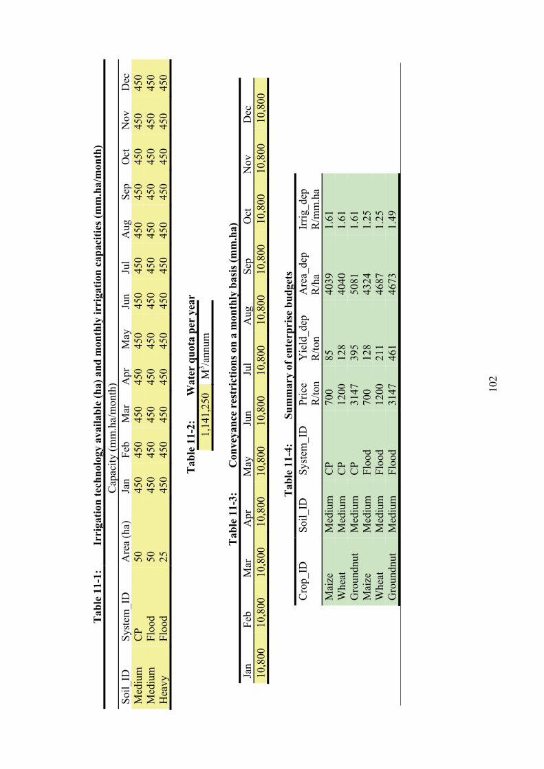
102
Tab
le 1
1-1:
Ir
riga
tion
tec
hn
olog
y av
aila
ble
(h
a) a
nd
mon
thly
irri
gati
on c
apac
itie
s (m
m.h
a/m
onth
)
Cap
acity
(m
m.h
a/m
onth
) S
oil_
ID
Sys
tem
_ID
A
rea
(ha)
Ja
n F
eb
Mar
A
pr
May
Ju
n Ju
l A
ug
Sep
O
ct
Nov
D
ec
Med
ium
C
P
50
450
450
450
450
450
450
450
450
450
450
450
450
Med
ium
F
lood
50
45
0 45
0 45
0 45
0 45
0 45
0 45
0 45
0 45
0 45
0 45
0 45
0 H
eavy
F
lood
25
45
0 45
0 45
0 45
0 45
0 45
0 45
0 45
0 45
0 45
0 45
0 45
0
Tab
le 1
1-2:
W
ater
qu
ota
per
yea
r
1,14
1,25
0
M3 /a
nnum
Tab
le 1
1-3:
C
onve
yan
ce r
estr
icti
ons
on a
mon
thly
bas
is (
mm
.ha)
Ja
n F
eb
Mar
A
pr
May
Ju
n Ju
l A
ug
Sep
O
ct
Nov
D
ec
10,8
00
10,8
00
10,8
00
10,8
00
10,8
00
10,8
00
10,8
00
10,8
00
10,8
00
10,8
00
10,8
00
10,8
00
T
able
11-
4:
Su
mm
ary
of e
nte
rpri
se b
ud
gets
C
rop_
ID
Soi
l_ID
S
yste
m_I
D
Pri
ce
Yie
ld_d
ep
Are
a_de
p Ir
rig_
dep
R
/ton
R/to
n R
/ha
R/m
m.h
a M
aize
M
ediu
m
CP
70
0 85
40
39
1.61
W
heat
M
ediu
m
CP
12
00
128
4040
1.
61
Gro
undn
ut
Med
ium
C
P
3147
39
5 50
81
1.61
M
aize
M
ediu
m
Flo
od
700
128
4324
1.
25
Whe
at
Med
ium
F
lood
12
00
211
4687
1.
25
Gro
undn
ut
Med
ium
F
lood
31
47
461
4673
1.
49

103
Tab
le 1
1-5:
Ir
riga
tion
req
uir
emen
t as
a f
un
ctio
n o
f cr
op, s
oil,
irri
gati
on s
ched
ule
an
d t
ech
nol
ogy
(mm
.ha)
C
rop_
ID
Soi
l_ID
S
ched
ule_
ID
Sys
tem
_ID
Ja
n F
eb
Mar
A
pr
May
Ju
n Ju
l A
ug
Sep
O
ct
Nov
D
ec
TO
TA
L
Mai
ze
Med
ium
1
CP
75
12
0 15
0 15
60
420
Whe
at
Med
ium
1
CP
15
45
90
195
210
30
58
5 G
roun
dnut
M
ediu
m
1 C
P
75
105
120
105
405
Mai
ze
Med
ium
1
Flo
od
60
240
240
60
12
0 72
0 W
heat
M
ediu
m
1 F
lood
60
120
120
240
300
30
87
0 G
roun
dnut
M
ediu
m
1 F
lood
12
0 12
0 24
0 24
0 60
60
84
0 M
aize
H
eavy
1
Flo
od
63
252
252
63
12
6 75
6 W
heat
H
eavy
1
Flo
od
63
12
6 12
6 25
2 31
5
32
914
Gro
undn
ut
Hea
vy
1 F
lood
12
6 12
6 25
2 25
2 63
63
88
2

104
Tab
le 1
1-6:
M
anag
emen
t op
tion
s C
rop_
ID
Mai
ze
Mai
ze
Whe
at
Whe
at
TO
TA
L
Soi
l_ID
M
ediu
m
Med
ium
M
ediu
m
Med
ium
Sch
edul
e_ID
1
1 1
1
Sys
tem
_ID
C
P
Flo
od
CP
F
lood
Are
a P
lant
ed (
ha)
50
50
50
50
100
E
con
omic
ou
tpu
t
Mar
gin
abov
e sp
ecif
ied
cost
( R
) 31
1940
31
7365
36
6532
35
5191
13
5102
9 C
rop
yiel
d (t
on/h
a)
10
10
7 7
7 W
UE
(to
n/m
m u
sed)
0.
023
0.02
3 0.
011
0.00
8 0.
0167
R
and/
mm
use
d 14
.85
15.1
1 12
.53
8.16
12
.66
Ir
riga
tion
wat
er u
se a
nd
con
veya
nce
cap
acit
ies
(mm
) C
omm
ents
Jan
3750
37
50
0 0
7500
Feb
60
00
6000
0
0 12
000
Cap
acit
y ex
ceed
ed
Mar
75
00
7500
0
0 15
000
Cap
acit
y ex
ceed
ed
Apr
75
0 75
0 0
0 15
00
M
ay
0 0
0 0
0
Jun
0 0
750
3000
37
50
Ju
l 0
0 22
50
6000
82
50
A
ug
0 0
4500
60
00
1050
0
Sep
0
0 97
50
1200
0 21
750
Cap
acit
y ex
ceed
ed
Oct
0
0 10
500
1500
0 25
500
Cap
acit
y ex
ceed
ed
Nov
0
0 15
00
0 15
00
D
ec
3000
30
00
0 15
00
7500
TO
TA
L
1147
50

105
Table 11-7 Wheat Centre Pivot WHEAT CENTRE PIVOT
Item Unit Price per Unit
Quantity Value per ha
Gross Income: *Wheat ton 1200 6.5 7800.00 Total 7800.00 Operating Costs: Area Dependant
Seed kg 6.36 100 636.00 7:2:3(31) + Zn kg 2.49 500 1245.00 KAN (28) kg 1.67 350 584.50 Omniboost kg 12.98 5 64.90 K P Max litre 7.70 1 7.70 10:1:6(20) liquid kg 1.53 190 290.70 Buctril DS litre 145.00 1 145.00 MCPA litre 51.00 0.5 25.50 Metasystox litre 117.00 0.5 58.50 Parathion litre 92.00 0.65 59.80 Granate EC litre 193.68 0.7 135.58 Crop dusting ha 95.00 2 190.00 Total 3443.18 Operating Costs: Yield Dependant
Contract Harvesting 715.00 Contract Transport 114.00 Total 829.00 Operating Costs: Other *Irrigation mm.ha 1.61 585 941.85 Fuel l 2.70 91.2 364.80 Reparations R 2.70 10% of
fuel 36.48
Lubricant R 2.70 2% of fuel
7.30
Insurance R 575.25 5.9% 575.25 Labour mandays 43.20 0.98 42.34 Interest R 279.04 1 279.04 Total 2274.05 ^Total Operating Costs 4635.53 ^Gross Margin 1280.77 Once the above information is provided, the user is allowed to evaluate the impact of alternative management options. A database of irrigation water requirements are generated with SAPWAT3 based on soil, irrigation system and irrigation schedule. The database is linked to the fixed resources of the farm and the economic parameters to determine the impact of alternative scenarios on key output variables to aid decision-making. A summary of the database generated with SAPWAT3 is provided in Table 11-5.
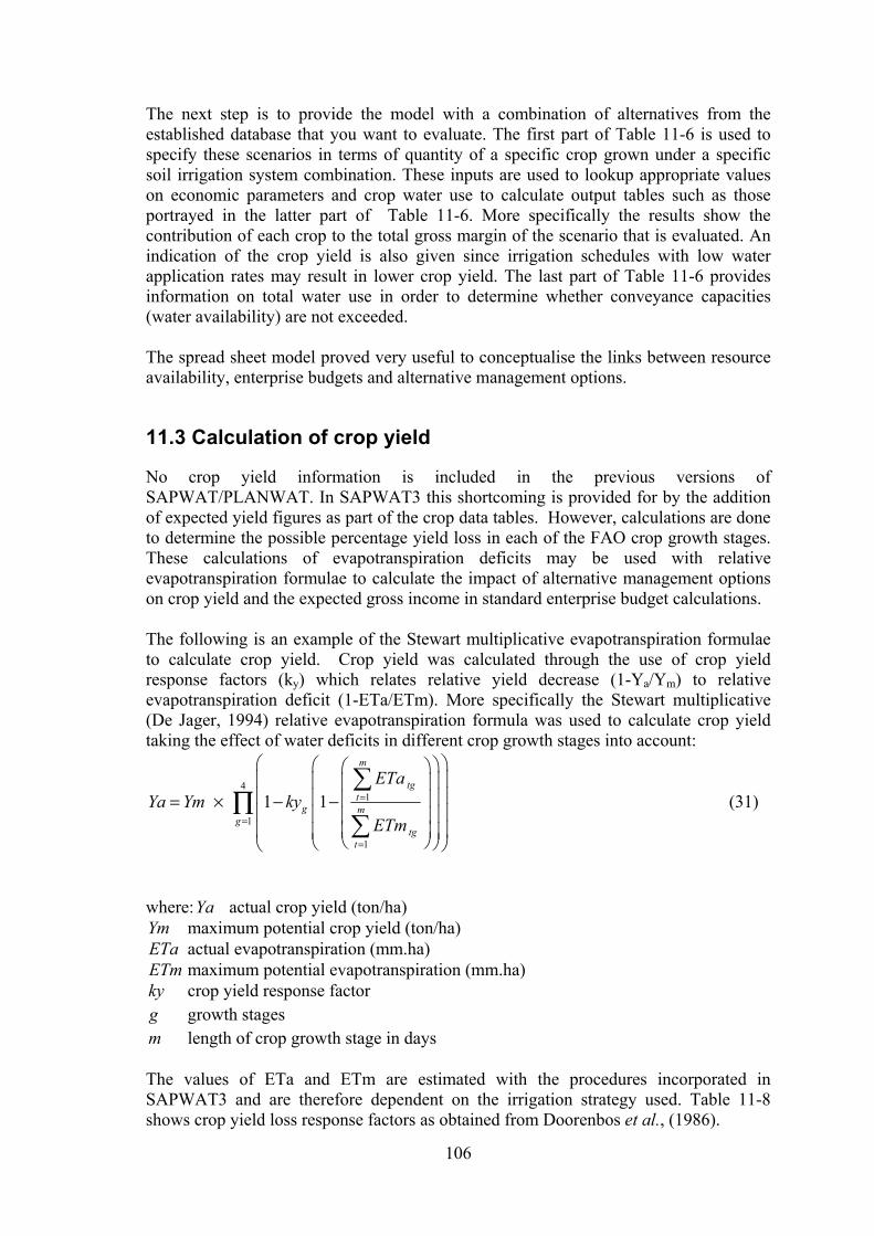
106
The next step is to provide the model with a combination of alternatives from the established database that you want to evaluate. The first part of Table 11-6 is used to specify these scenarios in terms of quantity of a specific crop grown under a specific soil irrigation system combination. These inputs are used to lookup appropriate values on economic parameters and crop water use to calculate output tables such as those portrayed in the latter part of Table 11-6. More specifically the results show the contribution of each crop to the total gross margin of the scenario that is evaluated. An indication of the crop yield is also given since irrigation schedules with low water application rates may result in lower crop yield. The last part of Table 11-6 provides information on total water use in order to determine whether conveyance capacities (water availability) are not exceeded. The spread sheet model proved very useful to conceptualise the links between resource availability, enterprise budgets and alternative management options.
11.3 Calculation of crop yield
No crop yield information is included in the previous versions of SAPWAT/PLANWAT. In SAPWAT3 this shortcoming is provided for by the addition of expected yield figures as part of the crop data tables. However, calculations are done to determine the possible percentage yield loss in each of the FAO crop growth stages. These calculations of evapotranspiration deficits may be used with relative evapotranspiration formulae to calculate the impact of alternative management options on crop yield and the expected gross income in standard enterprise budget calculations. The following is an example of the Stewart multiplicative evapotranspiration formulae to calculate crop yield. Crop yield was calculated through the use of crop yield response factors (ky) which relates relative yield decrease (1-Ya/Ym) to relative evapotranspiration deficit (1-ETa/ETm). More specifically the Stewart multiplicative (De Jager, 1994) relative evapotranspiration formula was used to calculate crop yield taking the effect of water deficits in different crop growth stages into account:
41
1
1
1 1
m
tgt
g mg
tgt
ETaYa Ym ky
ETm
(31)
where:Ya actual crop yield (ton/ha) Ym maximum potential crop yield (ton/ha) ETa actual evapotranspiration (mm.ha) ETm maximum potential evapotranspiration (mm.ha) ky crop yield response factor g growth stages m length of crop growth stage in days The values of ETa and ETm are estimated with the procedures incorporated in SAPWAT3 and are therefore dependent on the irrigation strategy used. Table 11-8 shows crop yield loss response factors as obtained from Doorenbos et al., (1986).

107
Table 11-8: Yield response factor (Doorenbos and Kassam, 1986) Crop Vegetative period Flowering
period Yield formation
Ripening Total growing period
Early Late Total
Banana 1.2-1.35Beans 0.2 1.1 0.75 0.2 1.15 Cabbage 0.2 0.45 0.6 0.95 Citrus 0.8-1.1 Cotton 0.2 0.5 0.25 0.85 Grapes 0.85 Groundnuts 0.2 0.8 0.6 0.2 0.7 Lucerne 0.7-1.1 0.7-1.1 Maize 0.4 1.5 0.5 0.2 1.25 Onion 0.45 0.8 0.3 1.1 Peas 0.2 0.9 0.7 0.2 1.15 Pepper 1.1 Potato 0.45 0.8 0.7 0.2 1.1 Safflower 0.3 0.55 0.6 0.8 Sorghum 0.2 0.55 0.45 0.2 0.9 Soybeans 0.2 0.8 1 0.85 Sugar beet Beet Sugar
0.6-1.0 0.7-1.1
Sugarcane 0.75 0.5 0.1 1.2 Sunflower 0.25 0.5 1.0 0.8 0.95 Tobacco 0.2 1.0 0.5 0.5 0.9 Tomatoes 0.4 1.1 0.8 0.4 1.05 Water melon
0.45 0.7 0.8 0.8 0.3 1.1
Wheat Spring
0.2
0.65
0.55
1.15
In the next section progress with respect to the programming of the Excel model in dBase programming language is reported.
11.4 Application in SAPWAT3
The economic module of SAPWAT3 is based on the construction of enterprise budgets and the application of activity analyses. However, the activity levels are not optimised. Rather, the user is given an indication of the activity levels that needs to be adjusted to improve the overall profitability of the farm plan given the availability of his most limiting resource. The activities consist of alternative crops grown in a specific Water User Association area (WUA) or on a farm with a given irrigation schedule. Resource availabilities that are considered are water, land, labour and production capital as well as water distribution capacities. Enterprise budgets are constructed for a specific crop with a given yield expectation. Cultivation and management practices are done so as to achieve the yield expectation.

108
SAPWAT3 gives an estimate of the crop yield expectation associated with a given irrigation management strategy. Enterprise budgets needs to be constructed for each alternative. Three different levels of complexity are included in the enterprise budgets to cater for users with different levels of available information. Table 1 gives an example of a detailed enterprise budget for wheat under centre pivot irrigation. The main categories of the enterprise budget are the gross income, area dependant operating cost, yield dependant operating cost and other operating cost. The costs are subtracted from the gross income to calculate the gross margin. In its most complex form the user will be allowed to generate a detailed enterprise budget based on calculation entities developed by Meiring (1994) as IRRICOST. The possibility to simplify IRRICOST procedures to calculate irrigation cost will be investigated. In its simplest form the user has to supply the module with sum totals for the main categories used. The information from the enterprise budgets is carried forward to a module to conduct activity analysis. The main objective of the activity analysis is to calculate the total gross margin of all the planned activity levels within the bounds of the available resources. In cases where resource availabilities are not specified the module calculates resource use to aid decision support. Procedures were developed to identify activities that should be increased to improve the total gross margin of the combined activity levels. The economic model was developed in Excel© and was then programmed to form part of SAPWAT3.
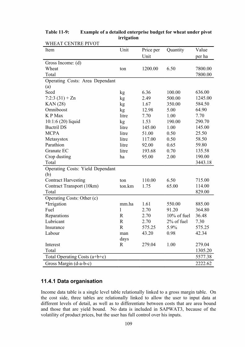
109
Table 11-9: Example of a detailed enterprise budget for wheat under pivot irrigation
WHEAT CENTRE PIVOT Item Unit Price per Quantity Value
Unit per ha Gross Income: (d) Wheat ton 1200.00 6.50 7800.00Total 7800.00Operating Costs: Area Dependant (a)
Seed kg 6.36 100.00 636.00 7:2:3 (31) + Zn kg 2.49 500.00 1245.00KAN (28) kg 1.67 350.00 584.50 Omniboost kg 12.98 5.00 64.90 K P Max litre 7.70 1.00 7.70 10:1:6 (20) liquid kg 1.53 190.00 290.70 Buctril DS litre 145.00 1.00 145.00 MCPA litre 51.00 0.50 25.50 Metasystox litre 117.00 0.50 58.50 Parathion litre 92.00 0.65 59.80 Granate EC litre 193.68 0.70 135.58 Crop dusting ha 95.00 2.00 190.00 Total 3443.18Operating Costs: Yield Dependant (b)
Contract Harvesting ton 110.00 6.50 715.00 Contract Transport (10km) ton.km 1.75 65.00 114.00 Total 829.00 Operating Costs: Other (c) *Irrigation mm.ha 1.61 550.00 885.00 Fuel l 2.70 91.20 364.80 Reparations R 2.70 10% of fuel 36.48 Lubricant R 2.70 2% of fuel 7.30 Insurance R 575.25 5.9% 575.25 Labour man
days 43.20 0.98 42.34
Interest R 279.04 1.00 279.04 Total 1305.20Total Operating Costs (a+b+c) 5577.38Gross Margin (d-a-b-c) 2222.62
11.4.1 Data organisation
Income data table is a single level table relationally linked to a gross margin table. On the cost side, three tables are relationally linked to allow the user to input data at different levels of detail, as well as to differentiate between costs that are area bound and those that are yield bound. No data is included in SAPWAT3, because of the volatility of product prices, but the user has full control over his inputs.

110
CHAPTER 12 WATER HARVESTING
12.1 Theoretical overview
12.1.1 Introduction
Water is one of the most essential requirements for the existence of living beings. However, as reported by several researchers (Southface, 2002; Coelho and Reddy, 2004 and Metro-water, 2005), urban areas are experiencing a decline of fresh water availability due to global climate change, population growth, urbanization, industrialization, pollution, lack of good governance and corruption. In many areas of the world, owing to the increase of population number in urban areas, conventional water supply systems have failed to meet the needs of the people (DTU, 1999). On the other hand, studies have shown that whilst all water is treated in urban areas to drinking water standards, as little as 1% of domestic water consumption is actually used for drinking and about 85% of bulk domestic water consumption goes to toilet flushing, laundry, and outdoor uses (Coombes, 2004). Investment in large scale and modern water supply schemes in rural areas also remains a challenge due to unique and scattered settlement patterns in most developing countries (Alem, 1999). The potential for new large-scale water resource development in developing countries is declining due to financial constraints, which leads to a growing interest in improving household water availability through the development of small-scale water sources (Ariyabandu, 2003). Reviving the traditional practices of the water harvesting system using scientific methods is a potential option for the looming water crisis (Alem, 1999; Metro-water, 2005). Roof water harvesting is an ancient technique for collecting and storing rainwater during the rainy season for later use (Finkel and Michael, 1995; cited by Alem, 1999; DTU, 1999; Gould and Nissen-Petersen, 1999; GDRC, 2005; Metro-water, 2005). Archaeological evidence verifies that the practice of rainwater harvesting goes back as far as 4000 years ago (DTU, 1999; Gould and Nissen-Petersen, 1999). Even nowadays, in many African countries, placing a small container under a roof to collect falling water during a rainy season is common practice (DTU, 1999). Rainwater harvesting is best known and practiced in the semi-arid areas where annual rainfall is in the range of between 400 and 600 mm (Alem, 1999). In arid and semi-arid regions, where precipitation is low or infrequent during the dry season, it is necessary to store the maximum amount of rainwater during the wet season, especially for agricultural and domestic water supply (OAS, 1997). The use of harvested rainwater for sanitary and drinking purpose is also a simple and cost effective way to meet the ever-increasing water demand in urban areas (Metro-water, 2005). Rainwater is valued for its purity and softness for human consumption, as well as for irrigation purposes (Gould and Nissen-Petersen, 1999). Furthermore, if maintenance of the rainwater harvesting system is undertaken regularly, it will ensure an effective long-term system operation (Sutherland and Fenn, 2000; Southface, 2002). Water storage tanks can be used for fish farming and the nutrient rich water from these tanks may even support sustainable agriculture by reducing the use of inorganic fertilizers (Rajesh et al., 2003).
111
Since traditional water supply technologies have been able to meet the needs of local populations for many centuries, the rainwater harvesting system is one of the options to ensure sustainability (Alem, 1999; Gould and Nissen-Petersen, 1999). Within the realm of credibility that it is likely to face water scarcity in the near future, the direct exploitation of rainwater as a source should not be ignored (Postel, 1992). Hence, it is necessary to take up measures to conserve and intensify the development of renewable water resources with all possible means at local and regional scale.
12.1.2 Domestic rainwater harvesting technology
The technology of domestic rainwater harvesting (DRWH) includes three main components: the catchment surface, the delivery system and a storage facility (Ariyabandu, 2003; Smet, 2003). Other possible components are filters or ‘first-flush’ diverters to reduce the quantity of debris entering the tank and other inlet and outlet devices to manage the water quality (Ariyabandu, 2003). As reported by Turner (2000) and DTU (2001b), the DRWH system reduces water-carrying time from point sources and increase household water consumption, which was previously constrained by the effort of collection. Other benefits of DRWH include reduction of soil erosion (especially in the hilly areas), and reduced amount of valuable energy inputs compared to the centralized water supply system. The design of a DRWH should take three considerations into account, namely social assessment, technical assessment and water demand assessment (Hailu and Merga; 2002). The social assessment includes the studying of the DRWH practices in the community, the opinion of the community on the use of the DRWH system and how much the households can afford to spend on a DRWH system. The technical assessment studies rainfall data, existing water sources, availability of construction materials and type, as well as size of potential harvesting surface areas. The water demand assessment investigates the available water supply throughout the dry season. This study does not include a social assessment of the DRWH system in the study area.
12.1.3 Catchment surface
The most common catchment surfaces for rainwater harvesting are the roofs of dwellings, courtyards, threshing areas, paved walking areas, plastic sheeting and trees (Ariyabandu, 2003). The roof of a building or a house is the first choice as catchment to harvest rainfall, although an open-sided barn can add additional capacity (Qiang and Yuanhong, 1999; Waskom, 2004; TWDB, 2005). The roof can be made of sheets of corrugated iron (CI), asbestos, or tiles of a wide variety, slate (thin layer of rock), and thatch that may be made of variety of organic materials (DTU, 1999). Water quality from different roof catchments is a result of the type of roof material, climatic conditions, and the environment (Vasudevan, 2002; cited by TWDB, 2005). Water collected from crude thatch would be coloured and turbid (Ariyabandu, 2003). Thatched roofs collection should be used only when no alternatives are available (Hailu and Merga, 2002). Natural soil, the threshing yard and roads have low efficiency in collecting rainwater (Qiang and Yuanhong, 1999). As reported by Smet (2003) and Waterfall (2004), paved catchments commonly have an overall run-off coefficient of 80%. The run-off coefficient for cement tiles is about 75%, while clay tiles usually collect less and has a run-off coefficient of 50%, depending on its production method. Plastic and metal

112
sheets do best with an efficiency of 80-90%. According to DTU (2001b), 90% or more of the rainwater collected on a CI roof will be drained to the storage tank if the gutter and down pipe system is properly fitted and maintained. The run-off coefficients for various catchment surfaces, as reported by different researchers, are given in Table 12-1.
Table 12-1 Run-off coefficients for various catchment surfaces TYPE OF CATCHMENT Pacey and Cullis (1989; cited by
Bhattacharya and Rane, 2003) DTU (2001b)
Roof catchments Tiles Corrugated iron sheets Thatched roof Asbestos sheet
0.8-0.9 0.7-0.9 - -
0.6-0.9 >0.9 0.2 0.8-0.9
Ground surface coverings Concrete Brick pavements
0.6-0.8 0.5-0.6
-
Untreated ground catchments Soil on slopes less than 10 percent Rocky natural catchments Green area
0.0-0.3 0.2-0.5 0.05-0.10
-
The efficiency of a roof catchment may be affected by the following factors (TWDB, 2005): The slope of the roof; Intensity of rainfall; Capacity of portion of the gutter which lies around the valley; Inadequate number of downspouts may also result in overrunning of gutters; Excessively long roof distances from ridge to eave; and Inadequate gutter maintenance. The typical components of which a DRWH system consists of are shown in Figure 12-1.

113
Figure 12-1 Typical rainwater harvesting system components (DTU, 1999)
12.1.4 Gutters
Gutters are part of the DRWH system that captures the rain falling on the roof and transfers it to the storage tank (Rees et al., 2000; Still and Thomas, 2002). There is a wide variety of shapes and forms of gutters ranging from factory made PVC pipes to traditional bamboo pipes or canvas and folded metals (Morgan, 1998; Rees et al., 2000). The most common materials used for gutters and downspouts are half-round PVC pipes, vinyl, seamless aluminium, and galvanized steel (TWDB, 2005). An ideal, gutter should be cheap to produce, efficient in capturing runoff water, easy to align and install, resistant to damage and simple to clean (Still and Thomas, 2002). Since the slightly acidic quality of rainwater could dissolve lead and thus contaminate the water, lead must not be used as gutter solders (DTU, 2001b). Low-cost gutter can also be made from a waterproof canvas (Morgan, 1998). Canvas material is the most suitable, being waterproof and resistant to degradation by the sun and thus has a longer life span than ordinary plastic sheeting (Morgan, 1998). Temporary gutters made of banana stems, aricunut trees, tin sheets and bamboo are also used in rural households of Sri Lanka (Lanka Rainwater Harvesting Forum, 2001). According to Still and Thomas (2002), if the design of gutters for CI roofs is adequate, it will be adequate for all other roof types. Even though intense rainfall requires guttering to hold relatively high flow capacities, u-shape (70 mm) or trapezoidal shape gutters are sufficient for most house roofs (Still and Thomas, 2002). Trapezoidal, semicircular and V-shaped gutters give similar economic performance in intercepting and conveying roof run-off water. Therefore the decision which to use can be made on the basis of ease of manufacture or its self-cleaning properties (Still and Thomas, 2002). V-shapes become blocked rather frequently and rectangular gutters do not make efficient use of material (Still and Thomas, 2002). A

114
trapezoidal or semi-circular shape gutter correctly sized for a roof slope of 22º will also be good for common roof slopes from 15º to over 30º, thus it is not necessary to know the roof slope when designing gutters (Still and Thomas, 2002). Other components, in addition to the horizontal gutters, are the drop outlet, at least two 45-degree elbows and brackets and straps to fasten the gutters and downspouts to the fascia and the wall (TWBD, 2005). Water leaving the roof may be collected at the edge or as directed jets, which in turn affects the interception of run-off. Other factors which may affect interception includes rainfall intensity, wind strength, gutter backing (fascia board), roof type, roof length, roof area, roof slope, excessively long roof distances from ridge to eave, concentrated flow from roof valley, straightness of the roof edge, the roof environment such as overhanging trees and inadequate gutter maintenance (Still and Thomas, 2002; TWDB, 2005). According to Still and Thomas (2002), the size of the gutter which is the most economic is the one that overflows when rainfall intensities reaches about 2 mm/min. This suggests that intensities up to 2 mm/min require a gutter aperture width of 100 mm outwards from the roof edge.
12.1.5 Down pipes
Down pipes of 40 mm internal diameter is sufficient if gutters are designed for a rainfall intensity of 2 mm/min. This is much smaller than the sizes commonly used in DRWH systems practice, which, according to Still and Thomas (2002), are oversized. Even a large building of 400 m2 does not need a down pipe larger than 75 mm internal diameter (Still and Thomas, 2002), if downspouts are located at about every 6.10 m. along the gutter, instead of the more common 12.20 m. This ensures that during heavy rains the gutter will not overflow (Gelt, 2005).
12.1.6 Water quality maintaining measures
A domestic rainwater harvesting system must be designed with consideration of some water quality maintenance measures (Ariyabandu, 2003). These measures can be: first flush diverters, covering lids, meshes and rapid in-situ water testing methods that indicate the presence of biological contamination.
12.1.6.1 Debris cleaning components
Leaf screens, leaf guards, funnel-type downspout filters, strainer baskets and filter socks are used to prevent debris entering the storage tank so that the potable water would be clean and to avoid the clogging of irrigation emitters (TWDB, 2005). Leaf screens prevent leaves from entering the storage tank and hence ensure high quality water. Leaf guards or screens are usually 0.63 cm mesh screens in wire frames that fit along the length of the gutter. Leaf guards/screens are usually necessary only in locations where trees overhang roofs. The funnel-type downspout filter is made of PVC or galvanized steel fitted with a stainless steel or brass screen. This type of filter offers the advantage of easy accessibility for cleaning. The funnel is cut into the downspout pipe at the same height or slightly higher than the highest water level in the storage tank.
12.1.6.2 First-flush diverters
According to Waskom (2004) and Rees et al. (2000), first-flush devices ensure a certain degree of better water quality in harvested rainwater. The first several litres of run-off from a gutter, roof, or other surface are likely to contain various impurities such as bird

115
droppings and dust. A first-flush device prevents this initial flow from draining into the storage tank. While leaf screens remove the larger debris, such as leaves, twigs, and blooms that fall on the roof, first-flush diverters get rid of the smaller contaminants, such as dust, pollen, and bird and rodent faeces (Rees et al., 2000). The quantity of first flush that will be diverted will be determined by the amount and the nature of accumulated contaminants, intensity of the rain event, the slope and smoothness of the collection surface (TWDB, 2005). According to TWDB (2005), the recommended diversion of first flush diverter ranges from 3.78 to 7.56 litres for each 9.3 m2 of collection area. If a gutter receives the quantity of run-off that require multiple downspouts, first-flush diversion devices will be required for each downspout. The simplest example of a first flush diverter is shown in Figure 12-2.
Figure 12-2 Standpipe first flush diverter (TWDB, 2005)
12.1.7 Storage facilities
The storage tank accounts for a large portion of the cost of a DRWH system (DTU, 2001b; TWDB, 2005). The variables such as the amount of rainwater, the water demand, the projected length of dry spells without rain, the catchment surface area, aesthetics, personal preference and economy or available budget are some of the factors that determine the budget and therefore the size of the storage tank (TWDB, 2005; Rees et al., 2000). Ideally, the DRWH collection system should involve basic construction techniques, be inexpensive to maintain, and have a long functional life span (Pacey and Cullis, 1985; cited by Turner, 2000). If the system is designed well, it should provide a good, safe source of drinking water at a relatively low cost when compared to the centralized water supply system (DTU, 2001b).

116
Figure 12-3 Water storage jar
Storage facilities such as mortar jars (Figure 12-3), ferro-cement jars, cylinders and cuboids of plastered brick, oil drums, corrugated iron cylinders, reinforced concrete tanks, or plastic drums for richer households, are commonly used in third world countries. Although the choice of tank construction material and storage size depends upon the available space, soil condition and economical factors, a storage tank should be of sufficient size, strong, impermeable, and durable and it should also have the ability to maintain water quality (DTU, 2001b; Ariyabandu, 2003). A potable water storage tank must satisfy the following conditions: It must be opaque so that algae growth is inhibited, it should be free from toxic substances, it should be covered to discourage mosquito breeding and it must be accessible for cleaning (TWDB, 2005). The construction of the tank may be above or below the ground surface, depending on the ease of construction and the decision made by the household (Turner, 2000). Aboveground storage are usually cheap; can be manufactured locally or can be purchased off the shelf; can be manufactured from a wide variety of materials and is easily constructed by using traditional materials. Furthermore, cracks or leakages are easily detected. On the other hand, a storage tank above the ground requires space; it must withstand different weather conditions and failure can be dangerous (Turner, 2000). According to Turner (2000), underground water storage tanks or cisterns are generally cheaper to construct, they have the advantage of using the surrounding ground as support, thus reducing the thickness required for the walls of the tank and it does not occupy space above ground level. On the other hand, water extraction is more problematic and often requires a pump, leaks or failures are more difficult to detect, contamination from groundwater is more common, tree roots may damage the structure, and there is danger to children and small animals if a tank cover is left open.
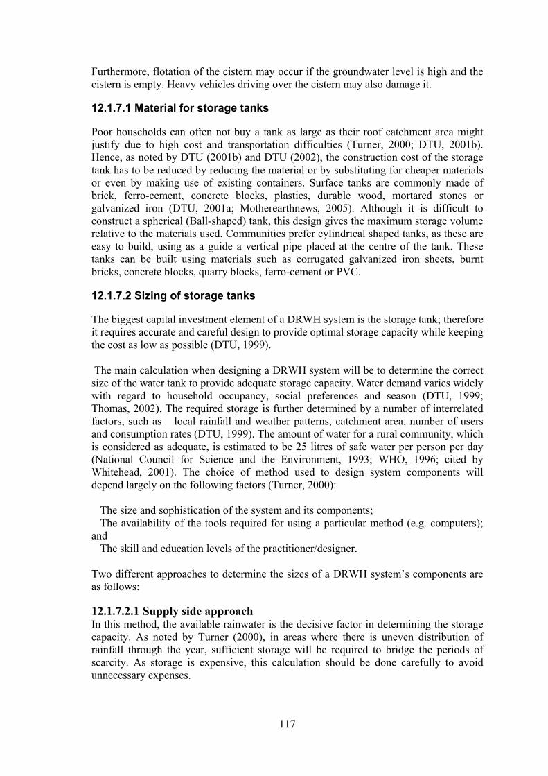
117
Furthermore, flotation of the cistern may occur if the groundwater level is high and the cistern is empty. Heavy vehicles driving over the cistern may also damage it.
12.1.7.1 Material for storage tanks
Poor households can often not buy a tank as large as their roof catchment area might justify due to high cost and transportation difficulties (Turner, 2000; DTU, 2001b). Hence, as noted by DTU (2001b) and DTU (2002), the construction cost of the storage tank has to be reduced by reducing the material or by substituting for cheaper materials or even by making use of existing containers. Surface tanks are commonly made of brick, ferro-cement, concrete blocks, plastics, durable wood, mortared stones or galvanized iron (DTU, 2001a; Motherearthnews, 2005). Although it is difficult to construct a spherical (Ball-shaped) tank, this design gives the maximum storage volume relative to the materials used. Communities prefer cylindrical shaped tanks, as these are easy to build, using as a guide a vertical pipe placed at the centre of the tank. These tanks can be built using materials such as corrugated galvanized iron sheets, burnt bricks, concrete blocks, quarry blocks, ferro-cement or PVC.
12.1.7.2 Sizing of storage tanks
The biggest capital investment element of a DRWH system is the storage tank; therefore it requires accurate and careful design to provide optimal storage capacity while keeping the cost as low as possible (DTU, 1999). The main calculation when designing a DRWH system will be to determine the correct size of the water tank to provide adequate storage capacity. Water demand varies widely with regard to household occupancy, social preferences and season (DTU, 1999; Thomas, 2002). The required storage is further determined by a number of interrelated factors, such as �local rainfall and weather patterns, catchment area, number of users and consumption rates (DTU, 1999). The amount of water for a rural community, which is considered as adequate, is estimated to be 25 litres of safe water per person per day (National Council for Science and the Environment, 1993; WHO, 1996; cited by Whitehead, 2001). The choice of method used to design system components will depend largely on the following factors (Turner, 2000): �The size and sophistication of the system and its components; �The availability of the tools required for using a particular method (e.g. computers); and �The skill and education levels of the practitioner/designer. Two different approaches to determine the sizes of a DRWH system’s components are as follows:
12.1.7.2.1 Supply side approach In this method, the available rainwater is the decisive factor in determining the storage capacity. As noted by Turner (2000), in areas where there is uneven distribution of rainfall through the year, sufficient storage will be required to bridge the periods of scarcity. As storage is expensive, this calculation should be done carefully to avoid unnecessary expenses.

118
12.1.7.2.2 Demand side approach In this approach, the number of persons per household and their water consumption is the decisive factor in determining the size of the storage capacity. The demand side approach is a simple method of calculation as the largest storage requirement is based on the consumption rates and occupancy of the building. This method assumes adequate and sufficient catchment area and rainfall and therefore is only applicable in areas where rainfall is more than adequate (Turner, 2000). There are also computer models available that determine the size of a rainwater storage system. The computer models simulate a rainwater harvesting system that will reliably meet demands. It finds the minimum catchment area and the smallest possible storage tank that will meet the demand with a probability of 95%, in spite of the fluctuations in the rainfall (Turner, 2000).
12.1.8 Low cost pumps
To lift water from the cistern to ground level or from the above ground storage to the irrigation field, an affordable and low cost pump is essential to replace manual lifting and carrying of water (Kay and Brabben, 2000; Brabben, 2001). Many existing pumps are regarded as over-designed and too expensive to incorporate into a DRWH system (Whitehead, 2001). These pumps are difficult to maintain because of the high cost of spares, and the spares may be stocked some distance from the pump location (Whitehead, 2001). Pumps for use on small scale irrigation farms need to be manageable, durable, have high hydraulic efficiencies, sufficient lifting height, be easy to manufacture and maintain with minimum skills and equipment and tools must be available in most local hardware outlets and markets (Whitehead, 2001). The labour-intensive rope and bucket method of lifting water for irrigation is the major production barrier for vegetable farmers in Africa (EWW, 2005). Irrigation time can be decreased by about a third or up to four hours per day if the farmer uses a treadle pump, which will allow the farmer to work on double of the original garden size (Kedge, 2001; EWW, 2005). For this reason, the treadle pump is gaining favour throughout Africa for rainwater harvesting and the reuse of grey water (EWW, 2005).
12.1.8.1 Treadle pump
The treadle pump (TP) is a human powered water pump that can lift irrigation water from source to point of use (Patrick and Stephenson, 1990; DTU, 1991). A treadle pump is simple and convenient to install, suitable for irrigating 0.5 ha of land, easy foot operated, can extract water from 7 m depth, can lift it up to about 12 m head and is capable of pumping 5000 litres of water per hour (SES, 2003; AOV International, 2005; EWW, 2005). The treadle pump was invented in the late 1970s in Bangladesh. Since then, the technology has been disseminated in many parts of the world from South East Asia to West Africa (Chancellor and O’Neill, 2000). The TP has been adapted for use in irrigation, where much greater volumes of water are needed (Kay and Brabben, 2000; Bennet, 2002). This simple, human-powered device can be manufactured and maintained at low-cost in rural workshops, it is relatively easy to repair, spare parts are readily available and improvisation is possible for application in developing countries (Chancellor and O’Neill, 2000; Kay, 2001). The introduction of TP’s into Africa also served as a useful tool for the introduction of irrigation technologies such as sprinkler and drip irrigation. These technologies result in increased crop yields as well as an increase in the area of land which can be farmed productively (Kay, 2001).

119
The principle of the TP is based on suction lift using a cylinder and piston to draw water from a source below ground level. Two pistons are used, each connected to a treadle (DTU, 1991; Kay and Brabben, 2000). The operator stands on the treadles, pressing the pistons up and down in a rhythmic motion as shown in Figure 12-4. There are two types of treadle pumps, the suction pump and the pressure pump (Kay and Brabben, 2000). The suction pump was made in Bangladesh for farmers who needed to lift large quantities of water through heights of 1-2 m and discharge it into a canal for gravity irrigation (Kay, 2001). The pressure pump works exactly on the same principle, but the delivery ends were modified so that water could be fed into a pipe under pressure for sprinklers, hoses or storage tanks (Kay and Brabben, 2000). According to Kedge (2001) and EWW (2001), suction pumps can raise water up to about 6-7 m head at a flow rate of up to 2 l/s, depending on the pump and the height above sea level. Pressure pumps can add an additional seven meters to the head on the delivery side, giving a total lift of about fourteen meters. Although the flow rate of the pressure pump is usually less and depends on the inlet and outlet pipe sizes and cylinder diameter, it is usually capable of pumping 1 l/s (Kay, 2001; Kedge, 2001). The pressure pump can discharge water up to a distance of approximately 150 m depending on friction losses and it is also better at lifting water from greater depths than the suction pump (Kedge, 2001). The pressure pump was developed to fulfil the needs of African farmers who often have to lift water from great depths and irrigate undulating land with sprinklers or hosepipes (Kay and Brabben, 2000). In theory the limits of a suction pump is 10.4 m at sea level, but in practice it reaches only up to 6.5 m. The suction head is also affected by change in temperature. An increase of 10°C in temperature decreases the suction head by 7%. Furthermore, for every thousand meters of elevation there is generally a loss of 1m suction head.
Figure 12-4 A Zambian farmer pumping water with a pressure treadle pump (Kedge, 2001)

120
The efficiency of the TP depends both on the physical strength of the operator and the ability to sustain this power over a period. According to Chancellor and O’Neill (2000), the typical rural peasant can produce a sustainable power of 40W and a comfortable discharge rate would therefore be around 50 l/min at a head of 3 m. At a head of 5 m, the discharge drops to 28 l/min.
12.1.8.2 Hand pump
In case of ground storage tanks low-level hand pumps may also be used for DRWH systems to extract water for drinking and domestic use (Whitehead, 2000). Figure 1.2.16 shows a hand pump used to extract water from a partially buried storage tank.
Figure 12-5: Hand pump (Whitehead, 2000)
12.1.9 Aquaculture
The harvested rainwater may also be used for aquaculture, depending on the availability of the rainwater. As reported by AquaSol (2003), the total world production of aquaculture, including aquatic plants, was more than 47.5 million tons by weight in 2000. The production of fish can easily be integrated into irrigation farming. It is based on the dual use of the same water, first for fish production and afterwards for irrigation (Cohen, 1996). Rajesh et al. (2003) reported that the nutrient rich water from aquaculture tanks might even support sustainable agriculture by reducing the use of inorganic fertilizers. Species such as Shrimp, Tilapia, Carp, Catfish, Salmon, Trout, Sea Bream, Mussels, Clams, Oysters, Scallops and many other aquatic organisms are all being actively farmed today (AquaSol, 2003). Any water-source could be used for fish farming, including underground water, water from the river, or from an impounding reservoir (Cohen, 1996). The scale and output of the aquaculture facilities are designed according to the water availability so as to cause no interference in the irrigation schedule (Cohen, 1996). During the dry season, due to a larger withdrawal of water for irrigation, the fish biomass increases in the reservoir and it results in an increased concentration of nitrogenous compounds from the fish excretion. This, in turn, may
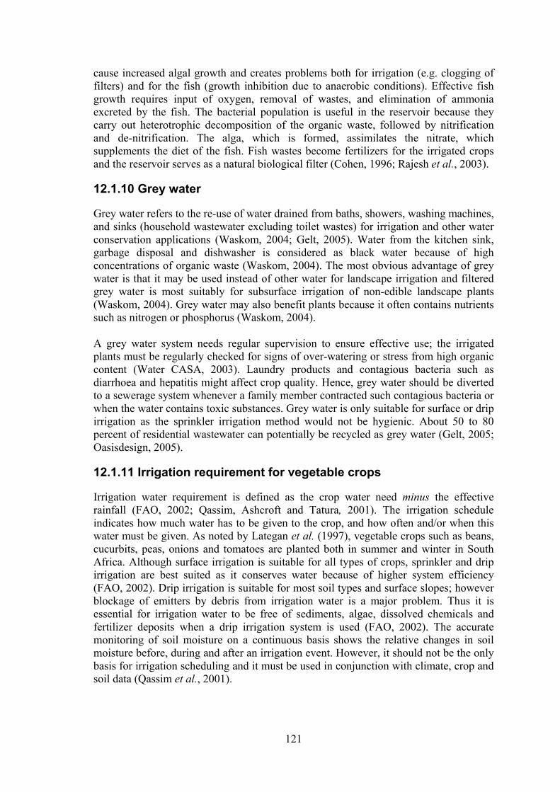
121
cause increased algal growth and creates problems both for irrigation (e.g. clogging of filters) and for the fish (growth inhibition due to anaerobic conditions). Effective fish growth requires input of oxygen, removal of wastes, and elimination of ammonia excreted by the fish. The bacterial population is useful in the reservoir because they carry out heterotrophic decomposition of the organic waste, followed by nitrification and de-nitrification. The alga, which is formed, assimilates the nitrate, which supplements the diet of the fish. Fish wastes become fertilizers for the irrigated crops and the reservoir serves as a natural biological filter (Cohen, 1996; Rajesh et al., 2003).
12.1.10 Grey water
Grey water refers to the re-use of water drained from baths, showers, washing machines, and sinks (household wastewater excluding toilet wastes) for irrigation and other water conservation applications (Waskom, 2004; Gelt, 2005). Water from the kitchen sink, garbage disposal and dishwasher is considered as black water because of high concentrations of organic waste (Waskom, 2004). The most obvious advantage of grey water is that it may be used instead of other water for landscape irrigation and filtered grey water is most suitably for subsurface irrigation of non-edible landscape plants (Waskom, 2004). Grey water may also benefit plants because it often contains nutrients such as nitrogen or phosphorus (Waskom, 2004). A grey water system needs regular supervision to ensure effective use; the irrigated plants must be regularly checked for signs of over-watering or stress from high organic content (Water CASA, 2003). Laundry products and contagious bacteria such as diarrhoea and hepatitis might affect crop quality. Hence, grey water should be diverted to a sewerage system whenever a family member contracted such contagious bacteria or when the water contains toxic substances. Grey water is only suitable for surface or drip irrigation as the sprinkler irrigation method would not be hygienic. About 50 to 80 percent of residential wastewater can potentially be recycled as grey water (Gelt, 2005; Oasisdesign, 2005).
12.1.11 Irrigation requirement for vegetable crops
Irrigation water requirement is defined as the crop water need minus the effective rainfall (FAO, 2002; Qassim, Ashcroft and Tatura, 2001). The irrigation schedule indicates how much water has to be given to the crop, and how often and/or when this water must be given. As noted by Lategan et al. (1997), vegetable crops such as beans, cucurbits, peas, onions and tomatoes are planted both in summer and winter in South Africa. Although surface irrigation is suitable for all types of crops, sprinkler and drip irrigation are best suited as it conserves water because of higher system efficiency (FAO, 2002). Drip irrigation is suitable for most soil types and surface slopes; however blockage of emitters by debris from irrigation water is a major problem. Thus it is essential for irrigation water to be free of sediments, algae, dissolved chemicals and fertilizer deposits when a drip irrigation system is used (FAO, 2002). The accurate monitoring of soil moisture on a continuous basis shows the relative changes in soil moisture before, during and after an irrigation event. However, it should not be the only basis for irrigation scheduling and it must be used in conjunction with climate, crop and soil data (Qassim et al., 2001).

122
12.1.12 Application of DRWH in SAPWAT3
The theory of rainwater harvesting is applied to the rainwater-harvesting module of SAPWAT3. The total water requirement is the sum of the estimated crop irrigation requirements and household requirements. Subtracting water available from other sources such as a well and grey water out of the household, reduces this total water requirement.

123
CHAPTER 13 COUNTRIES
A countries data file is included for the purpose of having outline maps available for each country for selection of weather stations. The basic information in this data file is the ISO alpha-3 country codes as described in ISO 3166, as well as the extreme northern, eastern, southern end western points of each country as these define the reference points to which weather stations are linked. These country maps are used for selecting weather stations for use in SAPWAT3. On the opening of the program the country taken up in the system files of the computer is selected as a default. The user can change this by selecting another country to work with.

124
CHAPTER 14 APPLYING SAPWAT3
14.1 Analysing irrigation strategies
14.1.1 The Dundee example
Figure 14-1 is the default irrigation management screen for maize planted near Dundee and presents the average situation for the full 50 year period. The default assumes that the soil profile is replenished every 7 days to 10mm below the upper limit (field capacity) during the growing season. Irrigation applications supplement rain shortfalls and are scheduled to ensure that the crop is provided with the exact water quantity required to match demand. While soil texture, rooting depth and system efficiency are taken into account the amount applied weekly is not limited and may be impractical.
Figure 14-1 Screen depicting the result of an irrigation requirement estimation run
for maize planted near Dundee
As shown in Figure 14-2, the estimated average irrigation water requirement is 467 mm of which 89 mm is due to evaporation. In order to simplify scheduling the run was repeated assuming that an irrigation system capable of applying up to 35 mm on a 10-day cycle was utilised and that irrigation be continued even when it rained! The applications every 10 days during stage one was 10 mm, during stage two 30 mm and from then on 35 mm. What sort of result could be anticipated? The average crop irrigation requirement at 455 mm is very similar as is the evaporation at 93 mm. It is possible to follow a season long mechanistic programme within the capacity of the system, but in very dry seasons there will be years when the crop will be stressed.
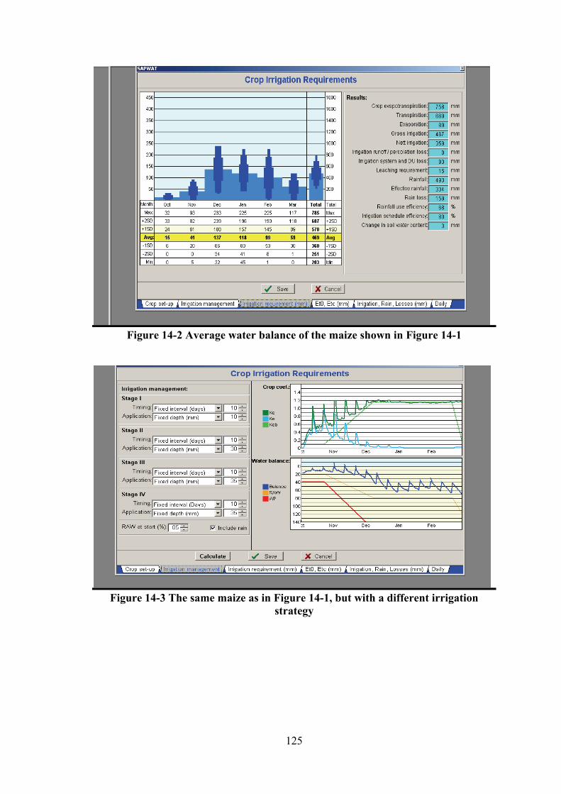
125
Figure 14-2 Average water balance of the maize shown in Figure 14-1
Figure 14-3 The same maize as in Figure 14-1, but with a different irrigation
strategy

126
Figure 14-4 The result of the irrigation strategy shown in Figure 14-3
The driest season was 1950/51 when only 300mm of rain fell during the growing season. In Jan, Feb and Mar the water content of the profile fell well below the RAW level (Figure 14-5). In order to cater for this, the farmer would need to increase irrigation in these months (always presuming that water is available!)
Figure 14-5 The result of a dry year for the same irrigation strategy as shown in
Figure 14-3
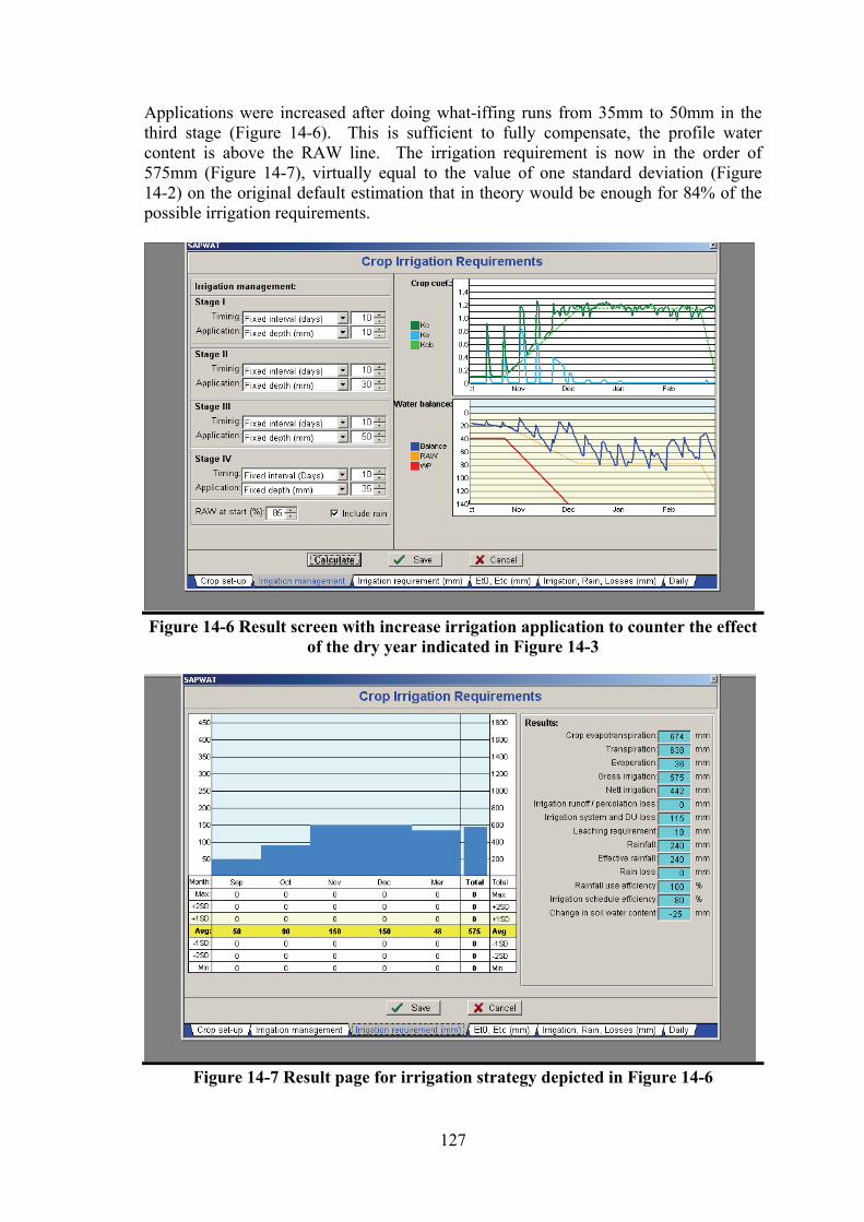
127
Applications were increased after doing what-iffing runs from 35mm to 50mm in the third stage (Figure 14-6). This is sufficient to fully compensate, the profile water content is above the RAW line. The irrigation requirement is now in the order of 575mm (Figure 14-7), virtually equal to the value of one standard deviation (Figure 14-2) on the original default estimation that in theory would be enough for 84% of the possible irrigation requirements.
Figure 14-6 Result screen with increase irrigation application to counter the effect
of the dry year indicated in Figure 14-3
Figure 14-7 Result page for irrigation strategy depicted in Figure 14-6

128
It is for the designer and farmer to decide on the capacity and characteristics of the irrigation as well as on management strategies. This process is further facilitated by examination of the detailed daily water balances provided for the full 50 years as seen in Figure 14-8.
Figure 14-8 Daily water balances. The marked areas indicate stress
The low rainfall season 1950/51 is selected showing the details of the water balance for the original pre-season programme. The application of 35mm/10d was inadequate in the third stage and the RZD (Root Zone Depletion) exceeded the RAW (Readily Available Water) marking the initiation of stress in early February. This is immediately noticeable by highlighting when scrolling through the full year. Other years when problems may arise in dry years can be identified by judicious scrolling.
14.1.2 The Douglas example
In this case the irrigation application was fixed at a more practical value – in the Dundee example the amount given per time was not always practical – and applied when soil water level reached a specific level. Figure 14-9 and Figure 14-10 show the result of a rooting depth of 1.2 m, while Figure 14-11 shows the result on a rooting depth of 600 mm.

129
Figure 14-9 Results of a fifty year run on maize in the Douglas area. Rooting depth = 1200mm
Figure 14-10 The result of a fifty year irrigation estimate run in Douglas on a strategy shown in Figure 14-9

130
Figure 14-11 Results of a fifty year run on maize in the Douglas area. Rooting depth = 900mm
Figure 14-12 The result of a fifty year irrigation estimate run in Douglas on a strategy shown in Figure 14-11

131
Figure 14-13 Results of a wet year (1957)
Figure 14-14 Results of a dry year (1994)
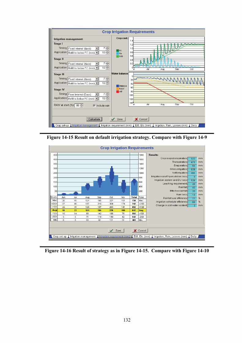
132
Figure 14-15 Result on default irrigation strategy. Compare with Figure 14-9
Figure 14-16 Result of strategy as in Figure 14-15. Compare with Figure 14-10

133
Figure 14-17 Result of default irrigation strategy. Compare with Figure 14-13 and Figure 14-14
Figure 14-18 Result of default irrigation strategy. Compare with Figure 14-13
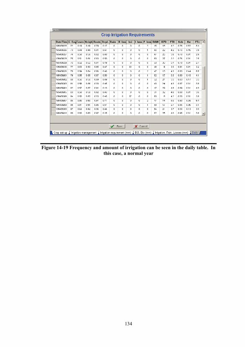
134
Figure 14-19 Frequency and amount of irrigation can be seen in the daily table. In this case, a normal year

135
REFERENCES
ALBERTSE, P. (2004). Personal communication. Stellenbosch, South Africa. ALLEN, R.G., PEREIRA, L.S., RAES, D. and SMITH, M. (1998). Crop evapotranspiration. Guidelines
for computing crop water requirements. Irrigation and Drainage Paper No 56. FAO. Rome, Italy. ALEM, G. (1999). Water harvesting in Ethiopia. 25th WEDC Conference, integrated developments for
water supply and sanitation. Water Engineering and Development Centre (WDEC), Loughborough University, UK, 387-390.
ANNANDALE, J.G., BENADÉ, N., JOVANOVIC, N.Z., STEYN, J.M. and DU SAUTOY, N. (1999). Facilitating Irrigation Scheduling by Means of the Soil Water Balance. WRC Report No 753/1/99. Water Research Commission, Pretoria. South Africa.
ANNANDALE, J.G., VAN DER WESTHUIZEN, A.J. and OLIVIER, F.C., (1996). Die Fasilitering van Tegnologie Oordrag deur Verbeterde Besproeiingsriglyne vir Groente en 'n Meganistiese Gewasmodeleringsbenadering. WRC Report No 476/1/96. Water Research Commission, Pretoria, South Africa.
AOV International (2005). Treadle pump. [Internet]. A government recognized export house, India. Available from: http://www.aovinternational.com/treadlepump.htm. [Accessed on 8 August 2005].
AQUASOL (2003). Fish farming. [Internet]. AquaSol Inc. USA. Available from: http://www.fishfarming.com/index.html. [Accessed on 11 August 2005].
ARIYABANDU, D.R. (2003). Very-low-cost domestic roofwater harvesting in the humid tropics. Report no: R4. Development Technology Unit, School of Engineering, University of Warwick, UK.
AUCAMP, J.D. (1978). Sigorei in die Oos-Kaap. PhD thesis. University of the Orange Free State, Bloemfontein, South Africa.
BENNET, D. (2002). Innovative Technology Transfer Framework Linked to Trade for UNIDO Action, United Nations Industrial Development Organization. Vienna, Austria.
BENNIE, A.T.P., STRYDOM, M.G. and VERY, H.S. (1998). Gerbuik van Rekenaarmodelle vir Landboukundige Waterbestuur op ekotoopvlak. WRC Report TT 102/98. Water Research Commission, Pretoria, South Africa.
BENNIE, A.T.P., VAN RENSBURG, L.D., STRYDOM, M.G. and DU PREEZ, C.C. (1997). Reaksie van Gewasse op Voorafgeprogrammeerde Tekortbesproeiing. WRC Report No 423/1/97. Water Research Commission, Pretoria, South Africa.
BHATTACHARYA, A. and RANE, O. (2003). Harvesting rainwater: catch water where it falls. Working Paper No. 0076. Center for Civil Society, India.
BRABBEN, T.E. (2001). Affordable Irrigation Technology: Prospects For smallholders in South Africa. SABI National congress, SABI, Johannesburg, South Africa.
BOEHLJE, M.D. and EIDMAN, V.R. (1984). Farm management. John Wiley and Sons, Inc. Canada. BOTHA, J.J., VAN RENSBURG, L.D., ANDERSON, J.J., HENSLEY, M., MACHELI, M.S., VAN
STADEN, P.P., KUNDHLANDE, G., GROENEWALD, D.G. and BAIPHETHI, M.N., 2003. Water Conservation Techniques on Small Plots in Semi-Arid Areas to Enhance Rainfall Use Efficiency, Food Security and Sustainable Crop Production. WRC Report No 1176/1/03. Water Research Commission. Pretoria. South Africa.
BOOYENS, A.J.D. (2004). Personal communication. Klerksdorp, South Africa. CERONIO, G. (2004). Personal communication. Free State University, Bloemfontein, South Africa. CHANCELLOR, F. and O’NEILL, D. (2000). The role of treadle pumps in changing the working and
economic environment of women irrigators: some considerations from Africa with particular reference to Zambia. ICID conference proceedings, RSA
CHILDS, R. (2002). Personal Communication. Port Elizabeth, South Africa. CHOW, V.T. (1959). Open Channel Hydraulics. McGraw-Hill, New York, USA COELHO, J. and REDDY, S.K. (2004). Making urban rainwater harvesting sustainable. Unpublished
Master’s Thesis. Department of Environment, Technology and Social Studies, University of Roskilde, India
COETZEE, A. (2004). Personal communication. GWK. Douglas, South Africa. COHEN, D. (1996). Integration of aquaculture and irrigation: rationale, principles and its practice in
Israel. 7th. International Conference on Water and Irrigation, Aquaculture Production Technology (Israel) Ltd, Israel
COOKE, D.A. and SCOTT, R.H. (1993). The Sugar Beet Crop. Chapman and Hall. London, Great Britain
COOMBES, P. (2004). Rain Water Tanks. Water Sensitive Planning Guide and Practice note for the Sydney region. Practice Note 4. Sydney region, Australia. 2-12
136
CROSBY, C.T. and CROSBY, C.P. (1999). A Computer Programme for Establishing Irrigation Requirements and Scheduling Strategies in Southern Africa. WRC Report No 624/1/99. Water Research Commission, Pretoria, South Africa
DAY, P.R., BOLT, G.H. and ANDERSON, (1967). Nature of soil water. Chapter 12 in HAGAN, R.M., HAISE, H.R. and EDMINSTER, T.W. (1967). Irrigation of Agricultural Lands. American Society of Agronomy, Madison, Wisconsin, USA
DE JAGER, J.M. (1994). Accuracy of vegetation evaporation ratio formulae for estimating final wheat yield. Water SA 20(4) 307-315
DE JAGER, J.M., MOTTRAM, R. and KENNEDY, J.A. (2001). Research on a Computerized Weather-based Irrigation Water Management System. WRC Report No 581/1/01. Water Research Commission, Pretoria, South Africa
DE JAGER, J.M. and VAN ZYL, W.H. (1987). Atmospheric Evaporative Demand and Evaporation Coefficient Concepts. Water SA, 15(2).
DE KOCK, G.C. (2004). Personal communication. Middelburg, South Africa. DICKINSON, E.B. and HYAM, G.F.S. (ED) (1984). The Pasture Handbook. Triomf Fertilizer Ltd.
Braamfontein, South Africa. DIPPENAAR, M. (2003). Pesonal communication. Rustenburg, South Africa. DOORENBOS, J. and PRUIT, W.O. (1977). Yield Response to Water. FAO Irrigation and Drainage
Paper no 24. FAO. Rome, Italy. DOORENBOS, J., KASSAM, A.H., BENTVELSEN, C.L.M, BRANSHEID, V., PLUSJÉ, J.M.G.A.,
SMITH, M., UITTENBOGAARD, G.O. and VAN DER WAL, H.K. (1986). Yield Response to Water. FAO Irrigation and Drainage Paper no 33. FAO. Rome. Italy.
DTU (1991). A human-powered pump for small-scale irrigation in developing countries. Working paper. Development Technology Unit, Department of Engineering, University of Warwick, Coventry, UK.
DTU (1999). Roof water harvesting, current technology for storing domestic rainwater. Report No. A1. School of Engineering, University of Warwick, Coventry, UK.
DTU (2001a.) Recommendations for designing rainwater harvesting system tanks. Report No. A4. Development Technology Unit, School of Engineering, University of Warwick, Coventry, UK.
DTU (2001b). Domestic roof water harvesting technology. [Internet]. Development Technology Unit, School of Engineering, University of Warwick, UK. Available from: http://www.eng.warwick.ac.uk/DTU/DRWH/components2.html [Accessed on 20 August 2005].
DTU (2002). New technology for very-low-cost domestic roof water harvesting. Development Technology, Unit School of Engineering, University of Warwick UK.
DU PLESSIS, J. (2003). Personal communication. Potchefstroom, South Africa. DU PREEZ, R. (2003). Personal communication. Burgershall, South Africa. DWAF (2003). Hydrological Information Systems. [Internet]. Department of Water Affairs and Forestry,
Pretoria, RSA. Available from: http://www.dwaf.gov.za/hydrology/cgi-bin/his/cgihis.exe/station [Accessed on 13 April 2004].
ENCYCLOPOEDIA BRITTANICA (2002). Brittanica.co.uk. London, UK. EWW (2001). Improved Manual Irrigation Component. Private irrigation pilot project. Nigerian Agency
for the promotion of private irrigation, Niger. FAO (2002). Irrigation Water Management Training Manuals. [Internet]. Land and Water development
division. Available from: http://www.fao.org/ag/AGL/AGLW/cropwater/training.stm. [Accessed on 12 December 2005].
FINKEL, and MICHAEL, S. (1995). Water harvesting. Proceedings of the SADC ELMS practical Workshop Windhoek and Okakarara, Namibia.
GARDNER, P.G., PEARCE, R.B. and MITCHELL, R.L. (1985). Physiology of Crop Plants. Iowa State University Press, Ames, Iowa, USA.
GARG, S.K. (1992). Irrigation Engineering and Hydraulics Structures. Khanna Publishers, Delhi, India. GDRC (2005). An introduction to rainwater harvest. [Internet]. Global Development Research Centre,
Japan. Available from: http://www.gdrc.org/uem/water/rainwater/introduction.html [Accessed on 27 May 2005].
GELT, J. (2005). Home Use of Grey water, Rainwater Conserves Water--and May Save Money. [Internet]. Water resources research centre college of agriculture and life science, The University of Arizona. Available from: http://ag.arizona.edu/AZWATER/arroyo/071rain.html. [Accessed on 6 December 2005].
GERBER, H. (2003). Personal communication. Upington, South Africa.

137
GOULD, J. and NISSEN-PETERSON, E. (1999). Rainwater catchment systems for domestic rainwater harvest design construction and implementation. [Internet]. Intermediate Technology Publications, UK. Available from: [Accessed on 2005].
GREEN, G.C. (1985). Estimating Irrigation Requirements of Crops. Research Institute for Soil and Irrigation, Pretoria, South Africa.
HAGAN, R.M., HAISE, H.R. and EDMINSTER, T.W. (1967). Irrigation of Agricultural Lands. American Society of Agronomy, Madison, Wisconsin, USA.
HAILU, M. and MERGA, S.N. (2002). The Experience of Water Harvesting in the Drylands of Ethiopia: Principles and Practices. Report No. 9. Drylands Coordination Group, Mekele, Ethiopia.
HOFFMAN, G.J., HOWELL, G.J. and SOLOMON, K.H. (1990). Management of farm irrigation systems. USA.
HOFFMAN, J.E. (2004). Personal communication, Stellenbosch, South Africa. INMAN-BAMBER, N.G. and MCGLINCHEY, M.G. (2003). Crop coefficients and water-use estimates
for sugarcane based on long-term Bowen ratio energy balance measurements. Field Crops Research, 2003, Vol. 83(2):125-138.
JANSEN, W. (2004). Personal communication. Vaalharts, South Africa. JOVANOVIC, N.Z. and ANNANDALE, J.G. (1999). An FAO type Crop Factor Modification to SWB
for Inclusion of Crops with Limited Data: Examples for Vegetable Crops. Water SA Vol. 25(2), April 1999. Pretoria. South Africa.
KAY, M. and BRABBEN, T. (2000). Treadle pumps for irrigation in Africa. Knowledge synthesis Report No. 1. International Program for Technology and Research in Irrigation and Drainage, Italy.
KAY, M. (2001). Smallholder Irrigation Technology Prospects for Sub-Saharan Africa. Knowledge synthesis Report No. 3. International Programme for Technology and Research in Irrigation and Drainage, IPTRID Secretariat Food and Agriculture Organization of the United Nations, Italy.
KEDGE, C. (2001). The Introduction of Treadle Pumps in to South Africa. SABI National congress, Institute for Agricultural Engineering, Johannesburg, RSA.
LANKA RAINWATER HARVESTING FORUM (2001). Household Water Security in Sri Lanka Using Domestic Roof Water Harvesting. Milestone1: Report D1. Lanka Rainwater Harvesting Forum, Sri Lanka.
LATEGAN, M.T., BURGER, J.H., HEYNS, P.J., KLEYNHANS, E.P.J, KOEGELENBERG, F.H., REINDERS, F.B. and SMAL, H.S. (1997). Crop Water Relationships and Climate. In: (ed.) -, Irrigation Design Manual, Ch. 4. Institute for Agricultural Engineering, Pretoria, South Africa.
LI, J. (1998). Modelling crop yield as affected by uniformity of sprinkler irrigation system. Agricultural Water Management, 38:135-146.
LECLER, N. (2004). Personal communication, Durban, South Africa. LIEBENBERG, A. (2002). Personal communication. Potchefstroom. South Africa. LUCKMAN, B. (2002). Personal Communication. Alexandria, South Africa. MALETIC, J.T. and HUTCHINS, T.B. (1967). Selection and classification of Irrigable Land. Chapter 10
in HAGAN, R.M., HAISE, H.R. and EDMINSTER, T.W. (1967). Irrigation of Agricultural Lands. American Society of Agronomy, Madison, Wisconsin, USA.
MAPPLEDORAM, B.D. (2004). Personal Communication. Pretoria, South Africa. McMAHON, M.J., KOFRANECK, A.M. and RUBATZKY, (2002). Hartmann’s Plant Science. Pearson
Education Inc. New Jersey, USA. MARAIS, D., RETHMAN, N.F.G. and ANNANDALE, J.G. (2002). Water Use and Water Use
Efficiency of Fodder Crops Under Irrigation. WRC Report No 573/1/02. Water Research Commission. Pretoria. South Africa.
MAYER, K. (2005). The dBASE Book. Authorhouse, Bloomington, Ind. USA. MAYER, K. (2007). The dBASE Reports. Authorhouse, Bloomington, Ind. USA. MEIRING, J.A. (1994). Die ontwikkeling en toepassing van 'n besluitnemingsondersteuningstelsel vir die
ekonomiese evaluering van risikobestuur op plaasvlak. PhD-thesis. Department Agricultural Economics, University of Free State, Bloemfontein. South Africa.
MEREDITH, D. (HON EDITOR) (1959). The Grasses and Pastures of South Africa. Central News Agency. Cape Town. South Africa.
METRO-WATER (2005). Rain water harvest. [Internet]. Chennai Metropolitan Water Supply and Sewerage Board. Available from: http://www.chennaimetrowater.com. [Accessed on 26 May 2005].
MORGAN, P. (1998). A low cost gutter technique using waterproof shade cloth for use in Rainwater Harvesting. [Internet]. Aquamor. Available from: http://aquamor.tripod.com/RAINWATER.htm. [Accessed on September 22 2005].

138
MORSE, R.L., ROBINSON, J.C. and FERREIRA, D.I. (1996). A Physiological Study of Six Banana Cultivars (Musa AAA; Cavedish Subgroup) in a Warm Subtropical Climate, Using in vitro Derived Planting Material. J. S.Afr. Soc. Hort. Sci 6 (2) December 1996. Pretoria. South Africa.
MOTHER EARTH NEWS (2005). Harvest the rain, mother earth news. [Internet]. Available from: http://www.motherearthnews.com/library/2003_August_September/Harvest_the_Rain#ccc. [Accessed on 17 Nov 2005].
MYBURGH, P.A. (2004a). Determining Grapevine Canopy Effects on Effective Rainfall. S. Afr. J. Enol. Vitic., Vol. 25(1), 2004.
MYBURGH, P.A. (2004b). ‘n Ondersoek na Moontlike Waterbesparing met Ondergrondse Besproeiing (Deel 1) – Besproeiingshoeveelhede, Benattingspatrone en Wortelverspreiding. Wynland Tydskrif. Februarie 2007.
MYBURG, P.A. and HOWELL, C.L. (2007a). Responses to Sunred Seedless and Muscat Supreme to Irrigation during Berry Ripening. Quality Aspects. SA Fruit Journal. Feb/March 2007.
MYBURG, P.A. and HOWELL, C.L. (2007b). Responses to Sunred Seedless and Muscat Supreme to Irrigation during Berry Ripening. Growth, Yield and Juice Analyses. SA Fruit Journal. Feb/March 2007.
NATIONAL COUNCIL FOR SCIENCE AND THE ENVIRONMENT (1993). Sustaining Water, Population and the Future of Renewable Water Supplies. [Internet]. Available from: http://www.cnie.org/pop/pai/h2o-toc.html. [Accessed on 13 December 2005].
NEL, A. (2003). Personal communication. Potchefstroom, South Africa. NETAFIM LANDBOUKUNDIGE AFDELING (2002). Die Beplanning van 'n Olyf Besproeiigstelsel.
Netafim South Africa (Pty) Ltd. Kraaifontein. South Africa. NORTH, M. (2004). Personal communication. Stellenbosch, South Africa. OAS (1997). Alternative Technologies for Freshwater Augmentation in Latin America and the
Caribbean. [Internet]. Unit of Sustainable Development and Environment of the General Secretariat of the Organization of American States, USA. Available from: http://www.oas.org/usde/publications/Unit/oea59e/begin.htm#Contents. [Accessed on 25 July 2005].
OASISDESIGN (2005). Grey Water Central. [Internet]. Available from: http://www.oasisdesign.net/greywater/index.htm. [Accessed on 13 December 2005].
OLIVIER, F. (2004). Personal communication. OTTO, W. (2004). Personal communication. Bethlehem. South Africa. PACEY, A. and CULLIS, A. (1985). Rainwater Harvesting. Intermediate Technology publications, UK. PACEY, A. and CULLIS, A. (1989). Rainwater Harvesting: The collection of rainfall and run-off in rural
areas. Intermediate Technology Publications, London, UK. PATRICK, N.S. and STEPHENSON, D. (1990). Spatial Variation of Rainfall Intensities for Short
Duration Storms. Hydrological Sciences Journal, 35(6): 667-680. POSTEL, S. (1992). Last Oasis: Facing Water Scarcity. [Internet]. W. W. Norton and Company.
Available from: http://dieoff.org/page29.htm. [Accessed on 29 November 2005]. QASSIM, A., ASHCROFT, B. and TATURA, (2001). Irrigation scheduling for vegetable crops.
Department of Primary Industries, ed., State of Victoria, Australia. QIANG, Z. and YUANHONG, L. (1999). Rainwater Harvesting in the Loess Plateau of Gansu, China
and its Significance. [Internet]. Gansu Research Institute for Water Conservancy, China. Available from: http://www.cpatsa.embrapa.br/servicos/catalogo/doc/wordwide/2_3_Zhu_Qiang.dc [Accessed on 3 August 2005].
RAE, A.N. (1994). Agricultural management economics: Activity analysis and decision making. Wallingford: CAB International.
RAJESH, K.M., MENDON, M.R., PRABHUDEVA, K.N. and PADIVAR, P.A. (2003). Aquaculture in reservoir fed canal based irrigation systems of India: A boon for fish production. Network of Aquaculture Centres in Asia-Pacific journal, 13(1):1-2.
READER'S DIGEST (1984). Illustrated Encyclopaedia of Gardening in South Africa. The Reader's Digest Association. Cape Town. South Africa.
REES, D.G., NVAKAANA, S. and THOMAS, T.H. (2000). Very-Low-Cost Roof water harvesting in east Africa: Domestic Rainwater Harvesting Research Program. Working Paper No. 55. Development Technology Unit, School of Engineering, University of Warwick, UK.
SANMUGNATHAN, K., HEUPERMAN, A., MALETTA, H., PRINZ, D., SALAS, P.A., THAKKER, H., SHEVAH, Y. and SMITH, L. (2000). Assessment of Irrigation Options, prepared as an input to the World Commission on Dams. Thematic Review IV.2 World Commission on Dams, Cape Town, RSA.

139
SCHULZE, R.E. and MAHARAJ, M. (2006). 50 Years of Daily Hydro-Climatic Data per Quaternary Catchment in South Africa. University of KwaZulu-Natal School of Bio-Resource Engineering and Environmental Hydrology. CD with data. Pietermaritzburg.
SENTRALE KATOENKOÖPERASIE (Undated). Katoen handleiding. Sentrale Katoenkoöperasie. Jan Kempdorp, Suid Afrika.
SES (2003). Treadle pump. [Internet]. Solar Engineering Service, South Africa. Available from: http://www.solarengineering.co.za. [Accessed on 8 August 2005]
SMET, J. (2003). Domestic Rainwater Harvesting. [Internet]. Water Engineering and Development Centre (WEDC), Loughborough University, UK. Available from: http://www.lboro.ac.uk/well/resources/fact-sheets/fact-sheets-htm/drh.htm [Accessed on 1 August 2005].
SMIT, M. (2003). Personal communication. Potchefstroom, South Africa. SMITH, M. (1991). Report on the Expert Consultation on Procedures for Revision of FAO Guidelines for
Prediction of Crop Water Requirements. FAO Land and Water development Division. FAO. Rome, Italy.
SMITH, M. (1992). CROPWAT, A Computer Programme for Irrigation Planning and Management. FAO Irrigation and Drainage Paper no 46. FAO. Rome, Italy.
SMITH, M. (1993). CLIMWAT for CROPWAT, a Climatic Data Base for Irrigation Planning and Management. FAO Irrigation and Drainage Paper No 49. FAO. Rome, Italy.
SMITH, M. (1994). Unpublished Duty Trip. Report, Pretoria, South Africa. FAO Land and Water Development Division. FAO. Rome, Italy.
SNEDECOR, G.W. and COCHRAN W.G., 1967. Statistical Methods. The Iowa State University Press. Ames. Iowa. USA. SOUTHFACE (2002). Water harvesting. Technical Bulletin 27. The Southface Energy Institute, Georgia
Atlanta, USA. STEYN, J.M. (2004). Personal Communication. Pretoria, South Africa. STILL, G.T. and THOMAS, T. (2002). The optimum sizing of gutters for domestic roof water harvesting.
Development Technology Unit, University of Warwick, UK. STRAHLER, A.H. and STRALER, A.N. (2002). Physical Geography: Science and Systems of the
Human Environment. John Wiley and Sons, Inc. New York, USA. STROOISNIJDER, L. (1987). Soil Evaporation: Test of a Practical Approach under Semi-Arid
Conditions. Neth. J. of Agric-Sc.i SUTHERLAND, D.C. and FENN, C.R. (2000). Assessment of Water Supply Options. Thematic Review
IV.3 prepared as an input to the World Commission on Dams. Secretariat of the World Commission on Dams, Cape Town, South Africa.
THERON, J. (2002). Personal communication. Glen, South Africa. THOMAS, T. (2002). DRWH performance predictor for use with coarse rainfall data. Report No.
DRWH04. School of Engineering, University of Warwick, UK. TOLMAY, C.D. and KRUGER, J.A. (Undated). Litchi Irrigation. Leaflet. Burgershall, South Africa. TURNER, S. (2000). Design of rainwater storage tanks for use in developing countries. Department of
Engineering, University of Warwick, UK, 76. TWDB (2005). The Texas Manual on Rain Water Harvesting. Texas Water Development Board, Texas,
USA. USWRC (1976). Guidelines for determining flood flow frequency. Bulletin #17. United States Water
Resources Council, Reston, VA, USA. VAN DER SCHYFF, J. (2004). Personal communication. Kynoch. Kimberley, South Africa. VAN HEERDEN, P.S. (2004). Estimating Irrigation requirements and Water Storage Requirements for
Farms, community Gardens and Backyard Gardens, and for Large Irrigation Systems: a user manual for PLANWAT version 1.2.3b and a CD-ROM to install the program. Working Paper 82. International Water Management Institute. Colombo, Sri Lanka.
VAN HEERDEN, P.S., CROSBY, C.T. and CROSBY, C.P. (2001). Using SAPWAT to Estimate Water Requirements of Crops in Selected Irrigation Areas Managed by the Orange-Vaal and Orange-Riet Water User Associations. WRC Report TT 163/01. Water Research Commission, Pretoria, South Africa.
VAN HEERDEN, P.S., CROSBY, C.T. and CROSBY, C.P. (1999). A computer program for establishing irrigation requirements and scheduling strategies in South Africa. WRC Report No. 624/1/99. Water Research Commission Pretoria, South Africa.
VAN RENSBURG, B.J. (2004). Personal communication. ARC. Vaalharts, South Africa. VAN WYK, W.F. (1992). Riglyne vir die verbouing van groente in die Transvaalstreek. Departement van
Landbou. Pretoria. South Africa.

140
VASUDEVAN, L. (2002). A study of biological contaminants in rainwater collected from rooftops in Bryan and College Station. Unpublished MSc thesis. A and M University, Texas, USA.
VIVIERS, J. (2003). Personal communication. VOLSCHENK, T., DE VILLIERS, J.F. and BEUKES, O. (2003). The Selection and Calibration of a
Model for Irrigation Scheduling of Deciduous Fruit Orchards. WRC Report 892/01/03. Water Research commission, Pretoria, South Africa.
WASKOM, R. (2004). Gray water Reuse and Rainwater Harvesting. [Internet]. Colorado State University Cooperative Extension. Available from: http://www.ext.colostate.edu/PUBS/natres/06702.html. [Accessed on 6 Dec 2005].
WATER CASA (2003). Residential Gray water reuse study. [Internet]. Water Conservation Alliance of Southern Arizona. Available from: http://www.watercasa.org/research/residential/fact.htm. [Accessed on 6 December 2005].
WATERFALL, P.H. (2004). Harvesting rainwater for landscape use. College of Agriculture and Life Sciences, University of Arizona, Arizona, USA.
WATT, S.B. (1978). Ferrocement Water Tanks and their Construction. IT Publications. WHITEHEAD, V. (2000). The Manufacture of Direct Action Handpumps for use with Domestic
Rainwater Harvesting Tanks. Report No.TR-DRWH09. Development Technology Unit, School of Engineering, University of Warwick, Coventry, UK.
WHITEHEAD, V. (2001). Development and Selection of Low Cost Hand pump for domestic Rainwater Water Tanks in East Africa. University of Warwick, UK.
WILKEN, L. (2004). Personal communication. Farmer. Douglas, South Africa. WHO (1996). Catalogue of Health Indicators. World health organization Geneva, Switzerland. ZIAD, A. (EDITOR) (1999). Date Palm Cultivation. FAO Plant Production and Protection Paper no 156.
FAO. Rome, Italy.