integrated process design, scheduling, and model

P RO C E S S S Y S T EM S E NG I N E E R I N G

Integrated process design, scheduling, and model predictivecontrol of batch processes with closed-loop implementation

Baris Burnak1,2 | Efstratios N. Pistikopoulos1,2

1Artie McFerrin Department of Chemical

Engineering, Texas A&M University, College

Station, Texas

2Texas A&M Energy Institute, Texas A&M

University College Station, College Station,

Texas

Correspondence

Efstratios N. Pistikopoulos, Texas A&M,

Energy Institute, Texas A&M University,

College Station, TX 77843, USA.

Email: [email protected]

Funding information

Energy Institute, Texas A and M University;

National Science Foundation, Grant/Award

Number: 1705423

Abstract

Simultaneous evaluation of multiple time scale decisions has been regarded as a

promising avenue to increase the process efficiency and profitability through leverag-

ing their synergistic interactions. Feasibility of such an integral approach is essential

to establish a guarantee for operability of the derived decisions. In this study, we pre-

sent a modeling methodology to integrate process design, scheduling, and advanced

control decisions with a single mixed-integer dynamic optimization (MIDO) formula-

tion while providing certificates of operability for the closed-loop implementation.

We use multi-parametric programming to derive explicit expressions for the model

predictive control strategy, which is embedded into the MIDO using the base-2

numeral system that enhances the computational tractability of the integrated prob-

lem by exponentially reducing the required number of binary variables. Moreover, we

apply the State Equipment Network representation within the MIDO to systemati-

cally evaluate the scheduling decisions. The proposed framework is illustrated with

two batch processes with different complexities.

K E YWORD S

batch process, model predictive control, multi-parametric programming, process design,

scheduling, state equipment network

1 | INTRODUCTION

Batch processing has been the predominant choice of operation

mode to manufacture high value specialty chemicals due to its

inherent flexibility to satisfy volatile customer requirements. Short

term scheduling in batch processing is a key factor toward deliver-

ing the targeted production requirements by the end of a pre-

determined horizon, as the scheduling implementation can often

dictate the profitability of the entire process especially if a high

number of products is to be manufactured in a limited number of

multipurpose equipment.1,2

A scheduling problem comprises a variety of decisions such as

resource allocation, task sequencing, and task timing. State-Task

Network (STN)3 and Resource-Task Network (RTN)4 are two of the

most widely used scheduling techniques that provide a systematic

modeling framework and solution strategy for these decisions

through mixed-integer linear programming (MILP). STN/RTN adopt a

recipe based scheduling approach, where the batch sizes and

processing times are assumed to be fixed. Continuous-time schedul-

ing approaches improve upon this limitation by using linearized rela-

tions for the batch sizes and processing times.2,5-10 However, the

optimality and even the feasibility of the schedule is susceptible to

internal and external influences such as different initial conditions,

known/unknown process disturbances, and fluctuations in utility

and raw material prices. Utilizing static transition tables that com-

prise processing times or time constants is a common, albeit ad-hoc

modeling representation that poses challenges to generalize for all

possible cases due to the lack of an in depth understanding of the

process dynamics.11

Model based approaches that integrate scheduling decisions with

faster time scale decisions are shown to be promising to account for

the dynamic characteristics of the process.12-17 Bhatia and Biegler18

Received: 15 March 2020 Revised: 3 June 2020 Accepted: 2 July 2020

DOI: 10.1002/aic.16981

AIChE J. 2020;e16981. wileyonlinelibrary.com/journal/aic © 2020 American Institute of Chemical Engineers 1 of 14

https://doi.org/10.1002/aic.16981

https://orcid.org/0000-0001-6118-8711

https://orcid.org/0000-0001-6220-818X

mailto:[email protected]

http://wileyonlinelibrary.com/journal/aic


have proposed one of the first significant contributions to simulta-

neously address the process design, scheduling, and optimal control of

a multipurpose batch process in a dynamic optimization formulation.

The authors formulated a dynamic model for the batch process in con-

tinuous time domain, which was discretized into a finite dimensional

nonlinear programming problem (NLP) and solved using orthogonal

collocation on finite elements. Biegler and co-workers extended the

use of dynamic models in an integrated formulation with more com-

prehensive and practically relevant scheduling schemes, state equip-

ment networks (SEN)19 and RTN.20 Chu and You21 have proposed a

surrogate modeling based approach for the integration planning,

scheduling, and open loop dynamic optimization for processes with

fixed batch sizes. More recently, Valdez-Navarro and Ricardez-

Sandoval22 have addressed the integrated scheduling and control

problem via the STN framework and a back-off algorithm to handle

process uncertainties. Although these approaches have been demon-

strated to capture the key interactions between the site level and unit

level process decisions, they are merely intended to be used in the

offline phase of decision making. In other words, such open loop opti-

mization approaches neglect the behavior of the feedback controller,

which fundamentally changes the dynamics of the process. Earlier

studies by Soroush and Kravaris23,24 accounted for the PID type state

feedback controllers by incorporating their explicit control laws in a

dynamic optimization formulation. Mohideen et al.25,26 used differen-

tial algebraic equation model to simultaneously determine the design

variables and the linear control structure under uncertainty, demon-

strated on a ternary distillation column. However, more advanced

control strategies such as constrained model predictive control (MPC)

have implicit forms, where the optimal control actions is only available

after solving an optimization problem at every step in a rolling horizon

manner. Brengel and Seider27 presented one of the first notable

efforts toward incorporating the MPC dynamics in dynamic design

optimization problem via a bi-level formulation, where the MPC prob-

lem was replaced by its complementary slackness conditions.

Ricardez-Sandoval and co-workers28,29 have proposed a stochastic

approach to integrate design optimization and MPC under uncertainty

by utilizing the probability distribution of the worst case disturbance

realizations. Zhuge and Ierapetritou30 developed multi-parametric

MPCs (mpMPC) to be incorporated in an integrated scheduling and

control formulation. However, the proposed approach utilizes an

event point based scheduling formulation with variable discretization

steps, which creates a mismatch with the fixed step size of the state

space model used in the mpMPC. Rossi et al.31 have proposed a two

phase architecture for the integrated problem where the first phase

solves a conventional scheduling problem offline and the second

phase comprises the online implementation of a modified nonlinear

MPC (NMPC). Koller and Ricardez-Sandoval32 have integrated the

process design, scheduling, and control problems in a dynamic model

and proposed a decomposition strategy based on flexibility and

feasibility analyses. Mora-Mariano et al. (2020)33 have incorporated

NMPC in an integrated large scale planning, scheduling, and control

problem and proposed a solution strategy based on Lagrangean

decomposition.

In this study, we introduce a modeling and optimization frame-

work through multi-parametric programming to embed linear MPC

dynamics into a mixed-integer dynamic optimization (MIDO) formula-

tion that simultaneously incorporates the process design, scheduling,

and control decisions. Accounting for linear MPC dynamics in the

integrated problem allows for the derivation of closed-loop optimal

trajectories that are attainable by the advanced control scheme,

thereby offering certificates of operability for the closed-loop imple-

mentation. We utilize the SEN framework for the scheduling problem

due to its suitability for the integration with the optimal control prob-

lem.19 Moreover, we introduce a methodology to exponentially

reduce the number of binary variables for embedding the piecewise

affine partitions derived from the multi-parametric solution of the lin-

ear MPC based on the base-2 numeral system.

The remainder of the paper is organized as follows. Section 2

defines the integrated problem and the types of decisions that are

considered in this study. In Section 3, we present a mathematical for-

mulation of the complete integrated problem, the methodology to

derive explicit MPC strategies that govern the system of interest, the

essential components of the SEN framework, and the methodology to

embed the explicit MPC solution into the resulting MIDO formulation.

Finally, we showcase the proposed approach with two batch process

examples in Section 4.

2 | PROBLEM STATEMENT

We consider a multipurpose batch process where the products are

allowed to follow different routes through the plant at different

times.34 The objective of these batch plants may vary depending on

the application, such as minimizing the cost, minimizing the makespan,

or maximizing the yield of a specific product. The goal of this work is

to present a unified theory and framework to determine simulta-

neously the following four levels of operational decisions, while deliv-

ering the target objective. Therefore, the problem statement is

illustrated in Figure 1 and outlined as follows.

2.1 | Given

First principle dynamics to manufacture the desired products

(preprocessing, reaction, and separation), any physical limitations

regarding the product quality and process safety, unit capital and

operating costs, and the range of demands on products.

2.2 | Determine

(a) Process design decisions: Dictates the capacity of the processing

units, (b) Process scheduling decisions: Includes task allocation, pro-

duction span or cycle, production sequence, and batch sizes, (c) Real-

time optimization decisions: Input and output trajectories that are

transmitted to the regulatory controller, and (d) Closed-loop control

2 of 14 BURNAK AND PISTIKOPOULOS

decisions: Linear MPC strategy that governs the process through the

control instruments.

2.3 | Objective

Minimize cost, minimize, makespan, maximize yield, and so on.

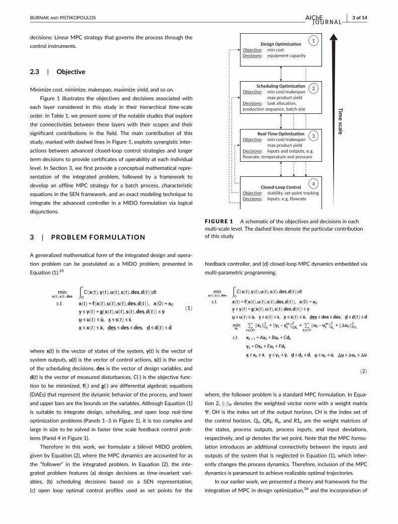
Figure 1 illustrates the objectives and decisions associated with

each layer considered in this study in their hierarchical time-scale

order. In Table 1, we present some of the notable studies that explore

the connectivities between these layers with their scopes and their

significant contributions in the field. The main contribution of this

study, marked with dashed lines in Figure 1, exploits synergistic inter-

actions between advanced closed-loop control strategies and longer

term decisions to provide certificates of operability at each individual

level. In Section 3, we first provide a conceptual mathematical repre-

sentation of the integrated problem, followed by a framework to

develop an offline MPC strategy for a batch process, characteristic

equations in the SEN framework, and an exact modeling technique to

integrate the advanced controller in a MIDO formulation via logical

disjunctions.

3 | PROBLEM FORMULATION

A generalized mathematical form of the integrated design and opera-

tion problem can be postulated as a MIDO problem, presented in

Equation (1).35

minu tð Þ,s tð Þ,des

ðτ0C x tð Þ,y tð Þ,u tð Þ,s tð Þ,des,d tð Þð Þdt

s:t: x tð Þ= f x tð Þ,u tð Þ,s tð Þ,des,d tð Þð Þ, x 0ð Þ= x0y≤ y tð Þ= g x tð Þ,u tð Þ,s tð Þ,des,d tð Þð Þ≤ �y

u≤u tð Þ≤ �u, s≤ s tð Þ≤�sx≤ x tð Þ≤ �x, des≤des≤ �des, d≤d tð Þ≤ �d

ð1Þ

where x(t) is the vector of states of the system, y(t) is the vector of

system outputs, u(t) is the vector of control actions, s(t) is the vector

of the scheduling decisions, des is the vector of design variables, and

d(t) is the vector of measured disturbances, C(�) is the objective func-

tion to be minimized, f(�) and g(�) are differential algebraic equations

(DAEs) that represent the dynamic behavior of the process, and lower

and upper bars are the bounds on the variables. Although Equation (1)

is suitable to integrate design, scheduling, and open loop real-time

optimization problems (Panels 1–3 in Figure 1), it is too complex and

large in size to be solved in faster time scale feedback control prob-

lems (Panel 4 in Figure 1).

Therefore in this work, we formulate a bilevel MIDO problem,

given by Equation (2), where the MPC dynamics are accounted for as

the “follower” in the integrated problem. In Equation (2), the inte-

grated problem features (a) design decisions as time-invariant vari-

ables, (b) scheduling decisions based on a SEN representation,

(c) open loop optimal control profiles used as set points for the

feedback controller, and (d) closed-loop MPC dynamics embedded via

multi-parametric programming.

minu tð Þ,s tð Þ,des

ðτ0C x tð Þ,y tð Þ,u tð Þ,s tð Þ,des,d tð Þð Þdt

s:t: x tð Þ= f x tð Þ,u tð Þ,s tð Þ,des,d tð Þð Þ, x 0ð Þ= x0y≤ y tð Þ= g x tð Þ,u tð Þ,s tð Þ,des,d tð Þð Þ≤ �yu≤u tð Þ≤ �u, s≤ s tð Þ≤�s, x≤ x tð Þ≤ �x, des≤des≤ �des, d≤d tð Þ≤ �d

minuk

Pk∈OH

kxkk2Qk+ kyk−yspk k

2QRk

+Pk∈CH

kuk−uspk k

2Rk+ kΔukk2R1k

s:t: xk +1 =Axk +Buk +Cdk

yk =Dxk + Euk + Fdk

x≤ xk ≤ �x, y≤ yk ≤ �y, d≤dk ≤ �d, u≤uk ≤ �u, Δu≤Δuk ≤Δ�u

ð2Þ

where, the follower problem is a standard MPC formulation. In Equa-

tion 2, k�kΨ denotes the weighted vector norm with a weight matrix

Ψ, OH is the index set of the output horizon, CH is the index set of

the control horizon, Qk, QRk, Rk, and R1k are the weight matrices of

the states, process outputs, process inputs, and input deviations,

respectively, and sp denotes the set point. Note that the MPC formu-

lation introduces an additional connectivity between the inputs and

outputs of the system that is neglected in Equation (1), which inher-

ently changes the process dynamics. Therefore, inclusion of the MPC

dynamics is paramount to achieve realizable optimal trajectories.

In our earlier work, we presented a theory and framework for the

integration of MPC in design optimization,36 and the incorporation of

F IGURE 1 A schematic of the objectives and decisions in eachmulti-scale level. The dashed lines denote the particular contributionof this study

BURNAK AND PISTIKOPOULOS 3 of 14

scheduling decisions via multi-parametric programming.37 Although

this theory is applicable to batch processes in principle, the practical

implementation becomes a challenging task as the control horizon and

the number of manipulated variables in the MPC scheme increase,

which is frequently encountered in batch processes. Increasing the

number of decision variables in the mpMPC formulation results in an

exponential increase in the number of critical regions, all of which

contain the optimal control law to be used based on the online state

measurements. In the integrated formulation presented in Equation (2),

the critical regions are embedded via a big-M or convex hull formula-

tion, requiring the use of a binary variable for each critical region

throughout the optimization horizon. In the following discussions, we

detail the constituents of the MIDO problem, that is, (a) mpMPC that

governs the units operations, (b) SEN formulation with its common

assumptions, (c) the integration of the mpMPC in the SEN and

dynamic optimization formulation. The complete formulation of the

MIDO is given in Supporting Information in a generic form.

3.1 | Developing the explicit MPC

Here, we detail the steps to develop a model based advanced control

strategy, illustrated by Panel 4 in Figure 1. The framework used in this

work to develop the explicit MPC has been introduced by

Pistikopoulos et al.38 with experimental validation of the methodology

on a smart metal hydride refueling system.39,40 The basic steps of the

framework can be summarized as (a) acquiring a high fidelity model

that represents the dynamics of the system of interest with sufficient

accuracy, (b) approximating the high fidelity model with discrete time

state space representations, (c) formulating an MPC based on the

approximate model and deriving its multi-parametric counterpart,

(d) validating the developed controller on the original high fidelity

model.

3.1.1 | Dynamic high fidelity modeling

A rigorous mathematical model is postulated based on first principles

and data-driven correlations in the form of a set of DAEs, as pres-

ented in Equation (3).

x tð Þ= f x tð Þ,u tð Þ,s tð Þ,des,d tð Þð Þ, x 0ð Þ= x0y tð Þ= g x tð Þ,u tð Þ,s tð Þ,des,d tð Þð Þ

ð3Þ

Equation (3) describes the relation between the degrees of freedom

and the observable outputs of the process via mass and energy bal-

ances, thermodynamic principles, and rate expressions. This mathemati-

cal model is directly incorporated in the MIDO formulation as presented

in Supporting Information. However, due to the continuous time

domain of the DAE system, the MIDO is infinite dimensional and hence

analytical solutions exist only for specific cases. Therefore in this study,

the continuous DAE is discretized via orthogonal collocation on finite

elements in the time steps of the MPC before solving the MIDO.

3.1.2 | Model approximation

The high fidelity model in Equation (3) is usually highly nonlinear for

chemical processing units, and hence imposes nonconvexities in the

context of an optimization problem. Therefore, we develop an

TABLE 1 An indicative list of the notable studies with their scopes

Authors

Design

decisions

Scheduling

decisions

Real-time

optimization

Closed-loop

control Significant contribution

Soroush

and Kravaris23,24✓ O ✓ ✓ Incorporated PID control in a DO formulation with

notions of feasibility, flexibility, controllability, and

safety.

Bhatia

and Biegler18✓ ✓ ✓ O Infinite dimensional DO is solved via ortogonal

collocation on finite elements.

Nie et al19 ✓ ✓ ✓ O Use of SEN for scheduling decisions.

Zhuge

and Ierapetritou53aO ✓ ✓ ✓ Closed-loop implementation with an iterative

approach.

Chu and You54 O ✓ ✓ O Stochastic programming and generalized benders

decomposition based approach.

Zhuge and

Ierapetritou30O ✓ ✓ ✓ Closed-loop strategies accounted for via multi-

parametric programming.

Nie et al20 ✓ ✓ ✓ O Use of RTN for scheduling decisions.

Du et al55a O ✓ ✓ ✓ Use of low-dimensional scale bridging models.

Baldea et al56a O ✓ ✓ ✓ Use of low-dimensional scale bridging models with

model-based control.

Valdez-Navarro and

Ricardez-Sandoval22O ✓ ✓ O Implemented back-off approach with Monte Carlo

simulations to account for uncertainty.

aCyclic continuous process—included in the list due the applicability of the approach to batch processes.


approximate model that mimics the dynamic behavior outlined by the

high fidelity model. Numerous approximation techniques have been

implemented to develop reduced order models to derive explicit MPC,

such as subspace identification, Box–Jenkins, Output Error, and Auto-

regressive Exogenous models.41 In this study, we use subspace identifi-

cation techniques via the MATLAB System Identification Toolbox,

which yields discrete time state space models in the following form.

xk +1 =Axk +Buk +Cdkyk =Dxk + Euk + Fdk ð4Þ

where yk is the predicted output at discrete time k. Note that multiple

state space models can be developed for different operating regions if

the process dynamics are highly nonlinear. Such ensemble models can

be used in tandem through a mixed-integer formulation in the MPC at

the cost of increasing the offline computational cost.37,42

3.1.3 | Developing explicit optimal control law

The approximate model in Equation (4) is used to develop the MPC

that governs the unit operations. The objectives of the MPC scheme

can include set-point tracking, maintaining the stability, generating

smooth control actions while satisfying any constraints on the process

inputs and outputs. Here, we derive the multi-parametric counterpart

of the MPC by treating the initial conditions, input–output set-points,

and measured disturbances as bounded parameters. This

reformulation43 yields an mpMPC scheme, where the optimal control

strategy is derived completely offline for the entire range of operation

as an explicit function of the parameters.44 The generic form of the

mpMPC problem is given in Equation (5).

uk θð Þ= argminuk

Xk∈OH

kxkk2Qk+ kyk−yspk k

2QRk

+Xk∈CH

kuk−uspk k2Rk+ kΔukk2R1k

s:t: xk + 1 =Axk +Buk +Cdk

yk =Dxk + Euk + Fdk

x≤ xk ≤ �x, y≤ yk ≤ �y, d≤dk ≤ �d

u≤uk ≤ �u, Δu≤Δuk ≤ �Δuθ = xk = 0,yk =0,uk = −1,dk ,y

spk ,u

spk

� �ð5Þ

Equation (5) is a multi-parametric quadratic programming (mpQP)

problem, which can be solved exactly by the POP Toolbox.45 The solution

of Equation (5) is expressed by a piece-wise affine function given in

Equation (6).

uk θð Þ=Knθ+ rn, 8θ∈CRn ð6aÞ

CRn≔ θ∈ΘjACRn θ≤ bCRn

n o, 8n∈NC ð6bÞ

where CRn is the nth critical region, Knθ + rn gives the affine control

law that yields the best solution in the parameter space bounded by

ACRn θ≤ bCRn , NC is the index set of the critical regions, and Θ is a closed

and bounded set. We note that if Equation (4) consists of multiple

state space models that represent mutually exclusive operating

regions, one can formulate a multi-parametric mixed-integer quadratic

programming (mpMIQP) problem, which can also be solved exactly,45

at the expense of increasing the number of critical regions of the

solution.

Here, the number of the critical regions and their dimensionality

are important aspects that directly correlate with the size of the inte-

grated problem. The potential maximum number of critical regions is a

direct result of the number of optimization variables and constraints

in Equation (5) and scales by nconst !nu ! nconst−nuð Þ!, where nconst is the number of

inequality constraints and nu is the number of linearly independent

optimization variables. The modeling technique to incorporate the

critical regions in the integrated problem, introduced in Section 3.3,

alleviates the computational burden of this inflation by using expo-

nentially less number of binary variables compared to conventional

big-M and convex hull relaxation schemes. The parameters θ, on the

other hand, increases the dimension of the polytopic representation

of the critical regions CR. Therefore, increasing the number of parame-

ters, such as accounting for more measured disturbances to the pro-

cess, results in a linear increase in the number of constraints in the

integrated problem given by Equation (2).

3.1.4 | Closed-loop validation

The piece-wise affine control law is implemented in the dynamic high-

fidelity model. The integrated model is subjected to rigorous testing

under numerous operating conditions and initial conditions to validate

the control strategy. We accept the mpMPC scheme if it performs

effective set-point tracking and stability. Otherwise, we tune the

weight matrices Qk, QRk, Rk, and R1k, increase the output and control

horizons, or develop a new approximate model. Here, we should note

that regardless of the potential improvements in the controller, a mis-

match between the open loop optimal trajectory and the closed-loop

profile is inevitable due to the approximate model used in the

mpMPC. The primary motivation of this study is to account for this

mismatch by generating a closed-loop optimal trajectory, while pre-

serving the benefits of the MPC.

3.2 | Scheduling using the SEN

In this section, we discuss the scheduling optimization via the SEN

representation outlined in Panel 2 of Figure 1. Nie et al.19 discussed

the suitability of the SEN framework for the integration of the sched-

uling decisions into a dynamic optimization formulation via general-

ized disjunctive programming. The authors adopted the unit specific

event-based continuous time representation, where the scheduling

horizon is divided into a finite number of event slots for each unit.

Although this approach is practical for open loop dynamic optimiza-

tion, it is a challenging task to apply on a process governed by an


MPC scheme due to two reasons. First, the bilevel nature of the inte-

grated problem poses a modeling challenge, which will be discussed in

Section 3.3. Second, the MPC strategy acts on the system in a rolling

horizon fashion, where the optimal control action is updated in dis-

crete time intervals, creating a mismatch with the continuous optimal

trajectory proposed by Nie et al.19 Since the discretization steps of

the MPC is fixed by design prior to operation, we use evenly distrib-

uted discrete time intervals in the SEN framework to integrate the

dynamic model and the mpMPC via logical disjunctions. In this part,

we discuss the essential constraints and objective functions that can

be used in the discrete-time SEN framework.

3.2.1 | Assignment constraints

We define a set of binary variables yj,s,t that denote operating

state s of an equipment j in time slot t. yj,s,t is equal to 1 if equip-

ment j is occupied by state s in time slot t, and 0 if otherwise.

Therefore, we use Equation (7a) to dictate the exclusivity of states

in an equipment throughout the scheduling time horizon. Similarly,

one task can only be executed in one equipment, as given by

Equation (7b).

Xs∈S

yj,s,t ≤1, 8j∈J ,8t∈T ð7aÞ

Xj∈J

yj,s,t ≤1, 8s∈S,8t∈T ð7bÞ

3.2.2 | Continuity constraints

After a task is assigned to an equipment, it has to continue the pro-

cess in the same equipment.

yj,s,t+1 ≤ yj,s,t, 8j∈J ,8s∈S,8t∈T ,t 6¼ tf ð8Þ

where tf is the final scheduling time step.

3.2.3 | Material balance

At each discretization point, we construct the material balance for

every component c to determine their availability, as presented in

Equation (9).

Ec,t = Ec,t−1 +Xj∈J

ΔEj,c,t, 8c∈C,8t∈T ,t>0 ð9Þ

where Ec,t denotes the amount of excess material of component c at

time t, and ΔEj,c,t is the generation or consumption term, dictated by

the reaction kinetics in the high-fidelity model.

3.2.4 | Capacity constraints

The vessel sizes limit the amount of material that can be processed in

every task.Xs∈S

yj,s,tV ≤Vj,t ≤Xs∈S

yj,s,tV, 8j∈J ,8t∈T ð10Þ

where Vj,t is a set of continuous variables that describe the volume

occupied in equipment j. Note that it is possible to enforce similar

constraints on the excess material Ec,t. However, we assume unlimited

intermediate storage (UIS) and neglect such constraints for simplicity.

3.2.5 | Quality constraints

These constraints are included to enforce certain quality metrics, such

as product purity or target demand, at the end of the batch. The

thresholds for these metrics are denoted by x*s .

x*s ≤ xs,t+1 +ℳ ws,tð Þ, 8s∈S*,t=0

x*s ≤ xs,t+1 +ℳ 1− ws,t−ws,t+1ð Þð Þ, 8s∈S*,8t∈T ,0≤ t≤ tfx*s ≤ xs,t+1 +ℳ 1−ws,tð Þ, 8s∈S*,t= tf

ð11Þ

where superscript “*” denotes the target states, ℳ is a sufficiently

large number for the big-M formulation, and ws,t is defined as a set of

linking variables between the scheduling model and the dynamic high

fidelity model. The linking variables ws,t are a set of Boolean variables

that are enforced to have a “true” value if the task is still in progress

via Equation (11), and “false” if otherwise. These variables are linked

to the scheduling model as presented by Equation (12).

t+1ð Þws,t ≤Xj0∈J

Xt0∈T

y j0 ,s,t0 , 8s∈S,8t∈T ð12Þ

3.2.6 | Sequence constraints

In the case that one state should take place only after the completion

of another task (e.g., precursors), the priority can be dictated by

Equation 13.

yj,s+ ,t ≤Xt

t0 =0

yj,s− ,t0 , 8j∈J ,8s−∈S− ,8s+∈S + ,8t∈T ð13Þ

where superscript “−” denotes the states that should be scheduled

earlier than the states labeled by the superscript “+.”

3.2.7 | Objective functions

Here, we will present two most commonly used objectives in a pro-

cess schedule, although they can be diversified and tailored to serve

different purposes. For makespan minimization, a set of Boolean vari-

ables zt is defined to indicate if the overall process is still in progress.


yj,s,t ≤ zt, 8j∈J ,8s∈S ð14Þ

Then, the makespan of one batch cycle can be minimized by mini-

mizing the sum of zt, that is,P

t∈T zt . Similarly, cost minimization is

one of the most common objectives encountered in processes sched-

ules, and can be expressed byP

t∈T Cuut +

Pt∈T C

tzt.

3.3 | Integrating mpMPC in the MIDO

In Section 3.1, we discussed a systematic procedure to develop MPC

schemes based on a high fidelity model, and to derive the explicit form

of the optimal control law, given by Equation (6). In this section, we

introduce an efficient methodology to integrate the optimal control

law with significantly less binary variables, which is previously out-

lined in Figure 1 with the dashed lines. The optimal control law is

expressed by a piecewise affine expression, and has two components,

namely (a) a set of affine functions that are optimal for the polytopic

space CRn (Equation (6a)), and (b) a set of polytopes that define the

space that bound the corresponding affine expression (Equation 6b).

Equation (6a) can be reformulated by using the two main relaxation

schemes, namely big-M reformulation and convex hull formulation.

These relaxation schemes can be used to embed the mpMPC to the

SEN network via a set of binary variables yCRn,t .

−ℳ 1−yCRn,t� �

≤ ut−Knθt− rn ≤ℳ 1−yCRn,t� �

, 8n∈NC,8t∈T ð15aÞ

−ℳ 1−yCRn,t� �

≤ un,t−Knθt−rn ≤ℳ 1−yCRn,t� �

, 8n∈NC,8t∈T ,

ut =Xn∈NC

un,t, 8t∈T

ð15bÞ

where Equation (15a) represents the big-M reformulation and Equa-

tion (15b) represents the convex hull reformulation for the optimal

control law. We also dictate that at most one critical region can be

selected at a given time throughout the scheduling horizon, that is,Pn∈NCy

CRn,t ≤1, 8t∈T . Selection of the critical region strictly depends

on the feasibility of the parameter set θt at time t according to Equa-

tion (6b). Therefore, we can simply relax the disjoint polytopes by

Equation (19).

ACRn θt−bCRn ≤ℳ 1−yCRn,t

� �, 8n∈NC,8t∈T ð16Þ

Note that both the big-M and convex hull reformulation

schemes require a binary variable for every critical region and for

each time step throughout the scheduling horizon. Consequently,

the computational complexity of the MIDO problem grow exponen-

tially as the number of critical regions of the explicit optimal control

law increase. The states of a batch process are inherently time-

varying and hence, the MPC scheme of a batch process requires lon-

ger output and control horizons, and larger bounds on the variables

compared to a typical continuous process. The combinatorial nature

of the increased number of variables and constraints of the MPC

problem results into an exponential increase in the number of critical

regions in its explicit solution. Therefore, employing the big-M and

convex hull reformulation techniques become impractical due to the

number of the yCRn,t variables, especially for the batch processes.

Herein, we present an efficient modeling technique with significantly

less binary variables using the base-2 numeral system. The goal of this

technique is to represent each critical region in a time step with a

unique combination of a set of binary variables, �yCRn2,t , where n2

denotes the nth critical region in the base-2 numeral system

(i.e., n2 = n). We treat the digits of n2 as an array of binary parameters,

denoted by βn2 . Therefore, a generic constraint g(x) can be relaxed

with the unique combinations of a set of binary variables yi as pres-

ented by Equation 17.

g xð Þ≤ℳX

i∈ mjβn2 ,m =0f gyi +

Xi∈ mjβn2 ,m =1f g

1−yið Þ

0B@

1CA ð17Þ

where, i ∈ ℐ is the index of the set of binary variables. The cardinality

of ℐ is given by jℐ j = dlog2ne, where j � j denotes the cardinality

operator and d�e denotes the ceiling function. Therefore, the relaxa-

tion scheme presented in Equation (17) reduces the number of

required binary variables from jNCj to dlog2| NCe. For example, log2, if

there are 8 constraints that need to be relaxed using big-M or convex

hull reformulation schemes, we have to use 8 binary variables to be

assigned for each constraint. However, the exact same relaxations can

be formulated by the proposed approach using 3 binary variables

instead. Similarly, 8 critical regions can be embedded in an upper level

optimization problem using 3 binary variables. Note that if the number

of binary combinations is greater than the number of constraints

(i.e., 2 log2nd e > n), we need additional constraints to exclude those com-

binations from the feasible space by integer cuts, as presented by

Equation (18).


yi−X

i∈ mjβn2 ,m =0f gyi ≤ jm j βn2,m =1 j −1 ð18Þ

An illustrative example for the use of base-2 numeral system to

relax a set of constraints is provided in Supporting Information.

3.3.1 | Using the base-2 numeral system tointegrate the explicit MPC solution

The base-2 numeral system can be applied to the big-M (15a) and

convex hull (15b) reformulation schemes for the piecewise affine con-

trol law as presented by Equations 19 and 20, respectively.

−ℳX

i∈ mjβn2 ,m =0f g�yCRi,t +


1−�yCRi,t� �

0B@

1CA≤ ut−Kn2θt−rn2 ,

8n2∈NC2,8t∈Tð19aÞ


ut−Kn2θt−rn2 ≤ℳX




0B@

1CA,

8n2∈NC2,8t∈T

ð19bÞ

−ℳX




0B@

1CA≤ un2,t−Kn2θt−rn2 ,

8n2∈NC2,8t∈Tð20aÞ

un2,t−Kn2θt−rn2 ≤ℳX




0B@

1CA,

8n2∈NC2,8t∈Tð20bÞ

ut =X

n2∈NC2

un2,t, 8t∈T ð20cÞ

Note that we do not enforceP

n∈NCyCRn,t ≤1,8t∈T in the base-2

numeral system as any feasible combination of the binary variables

�yCRn2,t yields a unique optimal control law. The feasibility of the control

laws in closed loop is analogously satisfied by Equation (21).

ACRn2θt−bCRn2 ≤ℳ

Xi∈ mjβn2,m =0f g

�yCRi,t +X

i∈ mjβn2,m =1f g1−�yCRi,t� �

0B@

1CA, 8n2∈NC2,8t∈T

ð21Þ

Therefore, using Equations (19) or (20) along with Equation 21

provides an exact integration of the mpMPC into the MIDO formula-

tion. If the number of critical regions n is greater than the number of

binary combinations (i.e., 2 log2nd e > n ), then we can use Equation (18)

by rewriting as follows to eliminate the infeasible combinations.


�yCRi,t −X

i∈ mjβn2 ,m =0f g�yCRi,t ≤ jm j βn2,m =1 j −1, t∈T ð22Þ

4 | CASE STUDIES

4.1 | Illustrative example—Single reaction

We consider a reaction that takes place in a batch reactor under non-

isothermal conditions. The goal of this case study is to demonstrate

the methodology to embed the MPC dynamics in a dynamic optimiza-

tion framework. Therefore, the design problem and scheduling via the

SEN framework are excluded in this problem for simplicity. Here, we

only focus on developing an MPC that manipulates the heat input to

track temperature and concentration set points that are determined

by the real-time optimization formulation. The stoichiometry of the

reaction is given as AÐk1k−1

B!k2 C, where A is the raw material, B is the

desired product, and C is a by-product with negligible monetary value.

The reaction setting is selected such that two of the most common

challenges in a batch reaction process, namely a reversible reaction

and a side reaction, are included. Due to the reverse reaction k−1,

complete conversion to product B is thermodynamically infeasible.

Furthermore, since the reaction path involves a by-product through

an irreversible reaction k2, the trivial solution of using an infinitely

long batch time at the maximum operable temperature is also infeasi-

ble to satisfy the product demand. Therefore, a model based dynamic

optimization approach should be employed to maximize the desired

performance metrics. In this case study, we will demonstrate

makespan minimization and yield maximization as performance

metrics.

The high-fidelity dynamics of the reaction is developed as a set of

DAE and the complete model is presented in Supporting Information.

4.1.1 | Open loop dynamic optimization foroptimal trajectories

Let the objective of the batch reaction be to produce a certain amount

of product B, while the batch time is minimized. A dynamic optimiza-

tion problem can be formulated to address such a makespan minimiza-

tion problem as presented by Equation 23.

minQ tð Þ

tf

s:t:1tf

1VdNc

dt=Xr∈ℛ

sc,r rr , 8c∈C

1tf

dTdt

=

−Pr∈ℛ

rrΔHr +Q=V

ρcpEqs: A:3 and A:4

NB t=1ð Þ ≥NdemB =0:4 kmol½ �, −12 kJ=h½ �≤Q tð Þ≤12 kJ=h½ �

NA t=0ð Þ=1:0 kmol½ �, NB t=0ð Þ=NC t=0ð Þ=0 kmol½ �, T t=0ð Þ=363 K½ �ð23Þ

where NdemB is the targeted amount of product at the end of the batch.

Here, the horizon of the problem is set as t = [0, 1], and the differen-

tial equations are scaled by tf, which denotes the batch time.

The dynamic optimization problem formulated in Equation (23) is

solved by orthogonal collocation on finite elements.46 The orthogonal

collocation formulation used in this work is based on Lagrange poly-

nomials and Radau roots. In this case study, we use 24 finite elements

(25 mesh points) with three collocation points for the differential and

algebraic variables. After discretization, the resulting NLP is solved by

the IPOPT solver.47 The optimal open loop profiles are determined as

presented in Figure 2, and the minimized makespan tf is 1.96 hr. The

calculated batch time assumes complete degrees of freedom over the

manipulated variables. However, practical applications often use

closed-loop controllers that manipulate such variables based on pro-

cess measurements and set points, which results in inherently differ-

ent process dynamics regardless of the efficacy of the controller.

Therefore, the only degrees of freedom in a closed-loop process are


the set point trajectories that are transmitted to the controller. The

following discussions will focus on (a) developing an MPC scheme for

the batch process described by Equations A.2a–A.4, (b) the effects of

the MPC dynamics on the closed-loop realization of the optimal open

loop profile, and (c) accounting for such effects in developing a realiz-

able optimal closed-loop profile.

4.1.2 | Developing an explicit MPC strategy forExample 1

We follow the procedure described in Section 3.1 to develop an

explicit MPC strategy based on the high fidelity model described by

Equations A.2a–A.4. A multitude of computational experiments are

conducted to generate the relevant data for system identification. In

each experiment, the input signal is based on a pseudo-random binary

sequence (PRBS) and randomized step amplitudes. Using the MATLAB

System Identification Toolbox, we develop the approximate state

space model, which is provided in Supporting Information.

Here, the identified model has one input variable, Q, two output

variables NB and T, and three identified states with no significant

physical meanings with a discretization step of 0.25 hr. The step

response of the identified model is provided in Supporting

Information.

The state space model is used in Equation (5) to construct the off-

line MPC formulation. The bounds on the variables and the tuning of

the weight matrices are provided in Supporting Information. Note that

the identified states do not have any bounds or weights in the objec-

tive function since they have no physical meanings. We also enforce

terminal constraints at the end of the output horizon to guarantee the

product quality at the process control level by using Equation (24).

0:99yspkf ≤ ykf ≤ 1:01yspkf ð30Þ

where ykf denotes the output variable at the end of the MPC output

horizon. In this case study, the output vector is defined as yk = [NB,k

Tk]T and [NB,k Tk]

T = [NB(t) T(t)]T at the discretization points. It is also

possible to use the product concentration NB,k/V to track product

quality instead of the amount of product NB,k, since direct measure-

ment of the component amount is not available to the operator. How-

ever, NB,k is used in this case study for simplicity since the two

quantities are linearly correlated and the reaction is operated under

constant volume. The vector of set points yspkf is treated as parameters

in the control problems and they are manipulated in the upper level

dynamic optimization formulation in the integrated problem.

The constructed mpMPC scheme is rearranged into a generic

mpQP problem via the YALMIP toolbox43 and solved by using the

POP toolbox45 in the MATLAB environment to derive the offline solu-

tion in the form of Equation (6). The resulting offline control law has

955 critical regions,1 which requires 955 binary variables for every

time step in the horizon to embed in an integrated problem via the

standard big-M or convex hull relaxation reformulations. Such a large

number of binary variables make the integrated problem intractable

even to determine a feasible solution. Therefore, we use the base-2

numeral system detailed in Section 3.3 to use 10 binary variables for

each time step instead. The developed mpMPC is integrated in the

high fidelity model for a closed-loop validation of the developed con-

trol law. The closed-loop system is tested rigorously with a set of

computational experiments, where the set points are changed arbi-

trarily, to observe the set point tracking efficacy of the controller.

Figure 3a presents a sample of a closed-loop simulation, where the

temperature set point changes after 7 hours in the operation. The

mpMPC scheme achieves satisfactory set point tracking within the

range of operation. However, it should be noted that any shift in the

operating set point results in a transition period where the states are

distant from the desired values, regardless of the effectiveness of the

controller. Open loop dynamic optimization approaches neglect any

feedback from the system during these transition periods and assume

perfect control over the process where the desired set points can be

tracked instantaneously. Neglecting the dynamics introduced by the

feedback controller may result in erroneous predictions of the process

if the process time introduced by the controller is significant com-

pared to the open loop system. Therefore, we subject the closed-loop

system to the open loop optimal set point trajectories presented in

Figure 2 to test the compatibility of the controller and operationally

relevant conditions. However, the closed-loop simulation fails to run

due to infeasible parameter realizations in the mpMPC during the

operation. The open loop optimal profile is unattainable for the con-

troller due to the terminal constraints given by Equation (24). There-

fore, we omit these terminal constraints to acquire a feasible closed-

loop profile, as presented in Figure 3(b). Here, we can observe that

the change in the temperature set point is in fact too steep for the

controller to track, resulting in infeasible parameter realizations. The

open loop optimal trajectory aims to produce the targeted 0.40 kmol/

m3 product B in 1.96 hr, while the achieved yield in closed-loop simu-

lation is 0.349 kmol/m3, indicating an error of 12.5% mismatch below

the desired amount. In other words, the infeasible parameter realiza-

tions stem from attempting to solve infeasible optimization problems.

Regardless of using an implicit linear MPC or its multiparametric

F IGURE 2 Open loop optimal profiles for the temperature,component concentrations, and heat input for Example 1 [Color figurecan be viewed at wileyonlinelibrary.com]


http://wileyonlinelibrary.com

counterpart, the feasible space of variables does not include a set of

solution that can satisfy all of the constraints simultaneously under

given process measurements and desired set points.

With the motivation to bridge the gap between the optimal tra-

jectories and the closed-loop realizations, we integrate the mpMPC

dynamics in the dynamic optimization formulation using the base-2

numeral system. The integrated model is first used to determine the

maximum possible yield in 2 hr (1.96 hr) using the given process and

the developed controller. The resulting MIDO problem is discretized

using eight finite elements (nine mesh points) with three collocation

points using the Pyomo environment.48-50 Note that each finite ele-

ment has a horizon of 0.25 hours, matching the discretization step of

the mpMPC. Discretizing the MIDO yields an MINLP problem with

80 binary variables, which is solved with GAMS/BARON51 with a

15 min limit on the solution time. The time limit is enforced to mimic

a real life application, where a decision has to be made periodically.

Accordingly, determining a feasible solution is prioritized over its opti-

mality to guarantee the operability of the process. Figure 4a shows

the closed-loop dynamic optimization profiles against its implementa-

tion on the original high fidelity model. Here, the optimal trajectory

and the optimal set points are two distinct entities. While the former

is the prediction of the closed-loop profile, the latter indicates the set

of operating points that are transmitted to the mpMPC. Notice that

the realization of the set points yields a similar profile to that

predicted by the dynamic optimization.

The solution of the MINLP indicates that the maximum possible

yield is 0.325 kmol/m3 at the end of the 2 hr horizon. This result

reveals that the original target of 0.40 kmol/m3 product B in

1.96 hours is in fact infeasible in closed-loop, although an open loop

optimal trajectory is attainable. The yield attained at the end of the

horizon is 0.314 kmol/m3 by simulating the closed-loop system

against the optimal trajectory, indicating an error of 3.4% mismatch.

(a) (b)

F IGURE 3 Closed-loop simulations of the process subjected to (a) arbitrarily changing set points (b) the optimal profile. The dashed linesdenote the set points [Color figure can be viewed at wileyonlinelibrary.com]

(a) (b)

F IGURE 4 Closed-loop dynamic optimization to maximize the yield of B in given time and the validation of the optimal profile against thehigh fidelity model. “Set points” denote the targets determined by the MIDO and used by the mpMPC in closed-loop, “Trajectory” represents theclosed-loop profile that is predicted by the MIDO, “Realization” denotes the actual closed-loop profile observed in the simulation [Color figurecan be viewed at wileyonlinelibrary.com]




Note that increasing the number of collocation points per finite ele-

ment may decrease the error at the expense of increasing the compu-

tational complexity.

In Figure 4b, the yield of product B is maximized for a horizon of

3 hr using the same explicit control strategy. In this problem, 12 finite

elements (13 mesh points) are used to maintain the horizon of each

individual element to 0.25 hr to match with the time steps of the

mpMPC. The dynamic optimization formulation predicts a yield of

0.367 kmol/m3, while the closed-loop simulation tracking the optimal

profile produces 0.363 kmol/m3 product B with an error of 1.1%.

The proposed integration methodology consistently bridges the

gap between the optimal profiles that are used as set points by the

controllers and the actual output of the closed-loop process, as dem-

onstrated in Figure 4. The explicit solution of the MPC scheme facili-

tates its exact implementation into a dynamic optimization

formulation. Moreover, the base-2 numeral system is used as a basis

for the relaxation of the piecewise affine critical regions, which ren-

dered the problem computationally tractable by exponentially reduc-

ing the required number of binary variables.

4.2 | Three reactions in two reactors

In this case study, we consider a system of three sets of reactions tak-

ing place in two reactors, where both reactors are capable of

processing the available tasks. The stoichiometry of the reactions is

given as AÐk1k−1

B!k2 C , A!k3 D, and B+D!k4 E , where the first reaction

set has the dynamics from the previous case study. In this example,

the valuable products are B, D, and E. Therefore, the operator has the

degree of freedom to select the most convenient task that delivers

the requirements of the desired objective at a given time. We employ

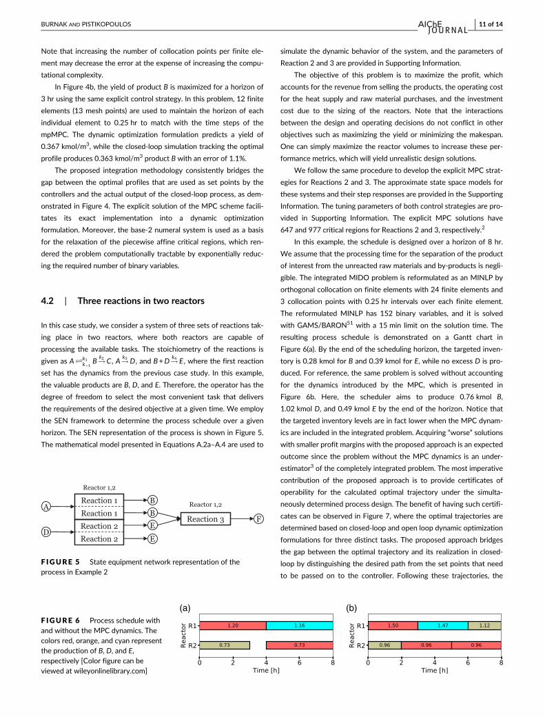
the SEN framework to determine the process schedule over a given

horizon. The SEN representation of the process is shown in Figure 5.

The mathematical model presented in Equations A.2a–A.4 are used to

simulate the dynamic behavior of the system, and the parameters of

Reaction 2 and 3 are provided in Supporting Information.

The objective of this problem is to maximize the profit, which

accounts for the revenue from selling the products, the operating cost

for the heat supply and raw material purchases, and the investment

cost due to the sizing of the reactors. Note that the interactions

between the design and operating decisions do not conflict in other

objectives such as maximizing the yield or minimizing the makespan.

One can simply maximize the reactor volumes to increase these per-

formance metrics, which will yield unrealistic design solutions.

We follow the same procedure to develop the explicit MPC strat-

egies for Reactions 2 and 3. The approximate state space models for

these systems and their step responses are provided in the Supporting

Information. The tuning parameters of both control strategies are pro-

vided in Supporting Information. The explicit MPC solutions have

647 and 977 critical regions for Reactions 2 and 3, respectively.2

In this example, the schedule is designed over a horizon of 8 hr.

We assume that the processing time for the separation of the product

of interest from the unreacted raw materials and by-products is negli-

gible. The integrated MIDO problem is reformulated as an MINLP by

orthogonal collocation on finite elements with 24 finite elements and

3 collocation points with 0.25 hr intervals over each finite element.

The reformulated MINLP has 152 binary variables, and it is solved

with GAMS/BARON51 with a 15 min limit on the solution time. The

resulting process schedule is demonstrated on a Gantt chart in

Figure 6(a). By the end of the scheduling horizon, the targeted inven-

tory is 0.28 kmol for B and 0.39 kmol for E, while no excess D is pro-

duced. For reference, the same problem is solved without accounting

for the dynamics introduced by the MPC, which is presented in

Figure 6b. Here, the scheduler aims to produce 0.76 kmol B,

1.02 kmol D, and 0.49 kmol E by the end of the horizon. Notice that

the targeted inventory levels are in fact lower when the MPC dynam-

ics are included in the integrated problem. Acquiring “worse” solutions

with smaller profit margins with the proposed approach is an expected

outcome since the problem without the MPC dynamics is an under-

estimator3 of the completely integrated problem. The most imperative

contribution of the proposed approach is to provide certificates of

operability for the calculated optimal trajectory under the simulta-

neously determined process design. The benefit of having such certifi-

cates can be observed in Figure 7, where the optimal trajectories are

determined based on closed-loop and open loop dynamic optimization

formulations for three distinct tasks. The proposed approach bridges

the gap between the optimal trajectory and its realization in closed-

loop by distinguishing the desired path from the set points that need

to be passed on to the controller. Following these trajectories, the

F IGURE 5 State equipment network representation of theprocess in Example 2

(a) (b)F IGURE 6 Process schedule withand without the MPC dynamics. Thecolors red, orange, and cyan representthe production of B, D, and E,respectively [Color figure can beviewed at wileyonlinelibrary.com]



proposed scheduling and control scheme achieves the targeted inven-

tory levels by producing 0.28 kmol B and 0.38 kmol E at the end of

the horizon. However, in the reference case, the controllers fail quite

often due to infeasible parameter realizations. The steep changes in

set points impose unrealistic trajectories for the controller, which can-

not satisfy the terminal constraints. Therefore, the closed-loop realiza-

tions in Figure 7b,d,f are simulated without enforcing the terminal

constraints in the MPC. Due to the mismatch between the set points

and the closed-loop realization, the targeted production cannot be

achieved in the dedicated time interval. In other words, the schedule

cannot be satisfied due to the delay in delivering the intended

amounts.

5 | CONCLUSION

In this work, we presented a modeling methodology to integrate the

process design, scheduling, and advanced control decisions in a single

(a) (b)

(c) (d)

(e) (f)

F IGURE 7 Closed-loop validation of the optimal input–output trajectories for three different tasks based on the closed-loop and open loopdynamic optimization formulations. Figures on the left hand side (a,c,e) show the optimal closed-loop trajectories, set-points that are passed on tothe MPC, and the closed-loop realizations. Figures on the right hand side (b,d,f) only show the optimal trajectories and their closed-looprealizations since the trajectories are used as the set points [Color figure can be viewed at wileyonlinelibrary.com]



optimization formulation for a batch process, while accounting for the

closed-loop operability. We introduced an exact formulation tech-

nique to integrate linear MPC dynamics into a MIDO problem by

multi-parametric programming. The piecewise affine expression that

represents the offline look-up table for the optimal control law is

embedded via the base-2 numeral system, which exponentially

reduced the required number of binary variables for the formulation.

The scheduling problem was formulated with the SEN framework due

to its suitability for the integration with dynamic optimization prob-

lems with dynamic optimization problems through logical disjunctions.

We showcased two case studies, the latter of which comprised all the

decision layers in the scope of this work, that is, process design,

scheduling, and control, with the objective to maximize the profit.

Although the closed-loop optimization predicts lower revenues and

higher costs than the open loop trajectories, the optimized profiles

were realized with significantly higher accuracy. Therefore, accounting

for the MPC dynamics is paramount to provide certificates of

operability.

Our future efforts will focus on addressing industrially relevant

batch processes, which are much larger in problem size. Although the

proposed methodology allows for finding a feasible solution, its opti-

mality still needs significant improvement to approach the global mini-

mum. Our future efforts will include two main avenues that can also

be used in tandem to improve the solution quality. First, the piecewise

affine control law is quadratic in the objective space. A tailored branch

and bound algorithm can be developed to fathom the infeasible or

suboptimal control laws by benefiting from the structure of the multi-

parametric solution space. Second, the open loop optimal trajectory is

an underestimator of the integrated problem. This solution can be

used in the tailored algorithm to achieve a better initial starting point.

Further improvement can be achieved by developing a more accurate

representation for the nonlinear effects of the design variables in the

process control level. In our earlier works,36,42,52 we accounted for

the design variables as added disturbances in the MPC scheme. How-

ever, highly nonlinear process design variables require piecewise

affine models that render the mpMPC problem into a multiparametric

mixed-integer quadratic program (mpMIQP), which significantly

increases the size of the offline look-up table. Our current efforts

focus on treating the design variables as left hand side parameters

instead of added disturbances to alleviate the computational burden

while handling highly nonlinear process designs.

ACKNOWLEDGMENTS

The authors acknowledge the financial support from the National Sci-

ence Foundation (Grant No. 1705423) and Energy Institute, Texas A

and M University.

CONFLICT OF INTEREST

The authors declare no conflict of interest.

ORCID

Baris Burnak https://orcid.org/0000-0001-6118-8711

Efstratios N. Pistikopoulos https://orcid.org/0000-0001-6220-818X

ENDNOTES1 The offline solution can be downloaded from http://paroc.tamu.edu/

http://paroc.tamu.edu/.2 The explicit MPC solutions can be downloaded from http://paroc.tamu.

edu/http://paroc.tamu.edu/.3 Underestimator is used in the direction of a conventionalminimization problem.

REFERENCES

1. Maravelias CT. General framework and modeling approach classifica-

tion for chemical production scheduling. AIChE J. 2012;58(6):1812-

1828. https://doi.org/10.1002/aic.13801.

2. Ierapetritou MG, Floudas CA. Effective continuous-time formulation

for short-term scheduling. 1. Multipurpose batch processes. Ind Eng

Chem Res. 1998;37(11):4341-4359.

3. Kondili E, Pantelides CC, Sargent RWH. A general algorithm for short-

term scheduling of batch operations—I. MILP formulation. Comput

Chem Eng. 1993;17(2):211-227.

4. Pantelides CC. Unified frameworks for optimal process planning and

scheduling. In: Proceedings on the Second Conference on Founda-

tions of Computer Aided Operations; 1993; New York: Cache Publi-

cations; p. 253-274.

5. Floudas CA, Lin X. Continuous-time versus discrete-time approaches

for scheduling of chemical processes: a review. Comput Chem Eng.

2004;28(11):2109-2129.

6. Maravelias CT, Grossmann IE. New general continuous-time state-

task network formulation for short-term scheduling of multipurpose

batch plants. Ind Eng Chem Res. 2003;42(13):3056-3074.

7. Seid R, Majozi T. A robust mathematical formulation for multipurpose

batch plants. Chem Eng Sci. 2012;68(1):36-53. http://www.

sciencedirect.com/science/article/pii/S0009250911006191.

8. Merchan AF, Maravelias CT. Reformulations of mixed-integer pro-

gramming continuous-time models for chemical production schedul-

ing. Ind Eng Chem Res. 2014;53(24):10155-10165.

9. Lee H, Maravelias CT. Combining the advantages of discrete- and

continuous-time scheduling models: part 1. Framework and mathe-

matical formulations. Comput Chem Eng. 2018;116:176-190.

10. Mostafaei H, Harjunkoski I. Continuous-time scheduling formulation

for multipurpose batch plants. AIChE J. 2020;66(2):e16804. https://

doi.org/10.1002/aic.16804.

11. Baldea M, Harjunkoski I. Integrated production scheduling and process

control: a systematic review. Comput Chem Eng. 2014;71:377-390.

12. Sakizlis V, Perkins JD, Pistikopoulos EN. Recent advances in

optimization-based simultaneous process and control design. Comput

Chem Eng. 2004;28(10):2069-2086.

13. Grossmann I. Enterprise-wide optimization: a new frontier in process

systems engineering. AIChE J. 2005;51(7):1846-1857.

14. Dias LS, Ierapetritou MG. From process control to supply chain man-

agement: an overview of integrated decision making strategies. Com-

put Chem Eng. 2017;106:826-835.

15. Burnak B, Diangelakis NA, Pistikopoulos EN. Towards the grand unifi-

cation of process design, scheduling, and control—utopia or reality? Pro-

cesses. 2019;7(7):461. https://www.mdpi.com/2227-9717/7/7/461.

16. Swartz CLE, Kawajiri Y. Design for dynamic operation - a review and

new perspectives for an increasingly dynamic plant operating envi-

ronment. Comput Chem Eng. 2019;128:329-339.

17. Rafiei M, Ricardez-Sandoval LA. New frontiers, challenges, and

opportunities in integration of design and control for enterprise-wide

sustainability. Comput Chem Eng. 2020;132:106610.

18. Bhatia T, Biegler L. Dynamic optimization in the design and scheduling of

multiproduct batch plants. Ind Eng Chem Res. 1996;5885(95):2234-2246.

19. Nie Y, Biegler LT, Wassick JM. Integrated scheduling and dynamic

optimization of batch processes using state equipment networks.

AIChE J. 2012;58(11):3416-3432.


https://orcid.org/0000-0001-6118-8711

https://orcid.org/0000-0001-6118-8711

https://orcid.org/0000-0001-6220-818X

https://orcid.org/0000-0001-6220-818X

http://paroc.tamu.edu/http://paroc.tamu.edu/





http://www.sciencedirect.com/science/article/pii/S0009250911006191

http://www.sciencedirect.com/science/article/pii/S0009250911006191



https://www.mdpi.com/2227-9717/7/7/461

20. Nie Y, Biegler LT, Wassick JM, Villa CM. Extended discrete-time resource

task network formulation for the reactive scheduling of a mixed

batch/continuous process. Ind Eng ChemRes. 2014;53(44):17112-17123.

21. Chu Y, You F. Integrated planning, scheduling, and dynamic optimiza-

tion for batch processes: MINLP model formulation and efficient

solution methods via surrogate modeling. Ind Eng Chem Res. 2014;53

(34):13391-13411. https://doi.org/10.1021/ie501986d.

22. Valdez-Navarro YI, Ricardez-Sandoval LA. A novel Back-off algorithm

for integration of scheduling and control of batch processes under

uncertainty. Ind Eng Chem Res. 2019;58(48):22064-22083.

23. Soroush M, Kravaris C. Optimal design and operation of batch reactors.

1. Theoretical framework. Ind Eng Chem Res. 1993;32(5):866-881.

24. Soroush M, Kravaris C. Optimal design and operation of batch reac-

tors. 2. A case study. Ind Eng Chem Res. 1993;32(5):882-893.

25. Mohideen MJ, Perkins JD, Pistikopoulos EN. Optimal synthesis and

design of dynamic systems under uncertainty. Comput Chem Eng.

1996;20(Suppl 2):S895-S900.

26. Mohideen MJ, Perkins JD, Pistikopoulos EN. Robust stability consid-

erations in optimal design of dynamic systems under uncertainty.

J Process Control. 1997;7(5):371-385.

27. Brengel DD, Seider WD. Coordinated design and control optimization

of nonlinear processes. Comput Chem Eng. 1992;16(9):861-886.

28. Sanchez-Sanchez KB, Ricardez-Sandoval LA. Simultaneous design and

control under uncertainty using model predictive control. Ind Eng

Chem Res. 2013;52(13):4815-4833.

29. Bahakim SS, Ricardez-Sandoval LA. Simultaneous design and MPC-

based control for dynamic systems under uncertainty: a stochastic

approach. Comput Chem Eng. 2014;63:66-81.

30. Zhuge J, Ierapetritou MG. Integration of scheduling and control for

batch processes using multi-parametric model predictive control.

AIChE J. 2014;60(9):3169-3183.

31. Rossi F, Casas-Orozco D, Reklaitis G, Manenti F, Buzzi-Ferraris G. A

computational framework for integrating campaign scheduling, dynamic

optimization and optimal control in multi-unit batch processes. Comput

Chem Eng. 2017;107:184-220. In honor of Professor Rafiqul Gani.

32. Koller RW, Ricardez-Sandoval LA, Biegler LT. Stochastic back-off algo-

rithm for simultaneous design, control, and scheduling of multiproduct

systems under uncertainty. AIChE J. 2018;64(7):2379-2389.

33. Mora-Mariano D, Gutiérrez-Limón MA, Flores-Tlacuahuac A. A

Lagrangean decomposition optimization approach for long-term plan-

ning, scheduling and control. Comput Chem Eng. 2020;135:106713.

34. Rippin DWT. Design and operation of multiproduct and multipurpose

batch chemical plants. — an analysis of problem structure. Comput

Chem Eng. 1983;7(4):463-481.

35. Bansal V, Sakizlis V, Ross R, Perkins JD, Pistikopoulos EN. New algo-

rithms for mixed-integer dynamic optimization. Comput Chem Eng.

2003;27(5):647-668.

36. Diangelakis NA, Burnak B, Katz J, Pistikopoulos EN. Process design

and control optimization: a simultaneous approach by multi-

parametric programming. AIChE J. 2017;63(11):4827-4846.

37. Burnak B, Diangelakis NA, Katz J, Pistikopoulos EN. Integrated pro-

cess design, scheduling, and control using multiparametric program-

ming. Comput Chem Eng. 2019;125:164-184.

38. Pistikopoulos EN, Diangelakis NA, Oberdieck R, Papathanasiou MM,

Nascu I, Sun M. PAROC – an integrated framework and software

platform for the optimisation and advanced model-based control of

process systems. Chem Eng Sci. 2015;136:115-138.

39. Ogumerem GS, Pistikopoulos EN. Parametric optimization and con-

trol toward the design of a smart metal hydride refueling system.

AIChE J. 2019;65(10):e16680.

40. Ogumerem GS. Application of Parametric Optimization and Control

in The Smart Manufacturing of Hydrogen Systems [PhD thesis]. Texas

A&M University; 2019.

41. Katz J, Burnak B, Pistikopoulos EN. The impact of model approxima-

tion in multiparametric model predictive control. Chem Eng Res Des.

2018;139:211-223.

42. Burnak B, Katz J, Diangelakis NA, Pistikopoulos EN. Simulta-

neous process scheduling and control: a multiparametric

programming-based approach. Ind Eng Chem Res. 2018;57(11):

3963-3976.

43. Löfberg J. YALMIP: a toolbox for modeling and optimization in

MATLAB. Proceedings of the IEEE International Symposium on

Computer-Aided Control System Design; 2004; pp. 284-289.

44. Dua P, Kouramas K, Dua V, Pistikopoulos EN. MPC on a chip—recent

advances on the application of multi-parametric model-based control.

Comput Chem Eng. 2008;32(4):754-765.

45. Oberdieck R, Diangelakis NA, Papathanasiou MM, Nascu I,

Pistikopoulos EN. POP - parametric optimization toolbox. Ind Eng

Chem Res. 2016;55(33):8979-8991.

46. Díaz MS, Biegler LT. Chapter 17—Dynamic optimization in process

systems. In: Martín MM, ed. Introduction to Software for Chemical

Engineers. second ed. Boca Raton, FL: CRC Press/Taylor & Francis;

2019:681-711.

47. Wächter A, Biegler LT. On the implementation of an interior-point fil-

ter line-search algorithm for large-scale nonlinear programming. Math

Program. 2006;106(1):25-57. https://doi.org/10.1007/s10107-004-

0559-y.

48. Hart WE, Watson JP, Woodruff DL. Pyomo: modeling and solving

mathematical programs in python. Math Program Comput. 2011;3(3):

219-260.

49. Hart WE, Laird CD, Watson JP, et al. Pyomo–Optimization Modeling in

Python. Vol 67. 2nd ed. New York: Springer Science & Business

Media; 2017.

50. Nicholson B, Siirola JD, Watson JP, Zavala VM, Biegler LT. Pyomo.

Dae: a modeling and automatic discretization framework for optimi-

zation with differential and algebraic equations. Math Program Com-

put. 2018;10(2):187-223.

51. Tawarmalani M, Sahinidis NV. A polyhedral branch-and-cut approach

to global optimization. Math Program. 2005;103:225-249.

52. Burnak B, Katz J, Diangelakis NA, Pistikopoulos EN. Integration of

design, scheduling, and control of combined heat and power systems:

a multiparametric programming based approach. Computer Aided

Chemical Engineering. Vol 44. Cambridge, MA: Elsevier; 2018:2203-

2208.

53. Zhuge J, Ierapetritou MG. Integration of scheduling and control with

closed loop implementation. Ind Eng Chem Res. 2012;51(25):8550-

8565.

54. Chu Y, You F. Integration of scheduling and dynamic optimization of

batch processes under uncertainty: two-stage stochastic program-

ming approach and enhanced generalized benders decomposition

algorithm. Ind Eng Chem Res. 2013;52(47):16851-16869. https://doi.

org/10.1021/ie402621t.

55. Du J, Park J, Harjunkoski I, Baldea M. A time scale-bridging approach

for integrating production scheduling and process control. Comput

Chem Eng. 2015;79:59-69.

56. Baldea M, Du J, Park J, Harjunkoski I. Integrated production schedul-

ing and model predictive control of continuous processes. AIChE J.

2015;61(12):4179-4190.

SUPPORTING INFORMATION

Additional supporting information may be found online in the

Supporting Information section at the end of this article.

How to cite this article: Burnak B, Pistikopoulos EN.

Integrated process design, scheduling, and model predictive

control of batch processes with closed-loop implementation.

AIChE J. 2020;e16981. https://doi.org/10.1002/aic.16981


https://doi.org/10.1021/ie501986d

https://doi.org/10.1007/s10107-004-0559-y

https://doi.org/10.1007/s10107-004-0559-y

https://doi.org/10.1021/ie402621t

https://doi.org/10.1021/ie402621t


integrated process design, scheduling, and model

Documents