Proceedings of ASME 2010 3rd Joint US-European Fluids Engineering Summer Meeting and 8th International Conference on Nanochannels, Microchannels, and Minichannels

FEDSM2010-ICNMM2010August 1-5, 2010, Montreal, Canada

FEDSM-ICNMM2010-31014

Integrated Motor/Propulsor Duct Optimization for Increased Vehicle and Propulsor Performance

Dr. Stephen A. Huyer and Amanda Dropkin

Naval Undersea Warfare Center Newport, RI, USA

Abstract:

Integrated electric motor/propulsor technological development offers the potential to increase usable volume for undersea vehicles by locating the electric motor in the duct. This has the added advantage that the electric motor has increased usable torque due to the increased radius. For many torpedo and unmanned undersea vehicle applications, however, the maximum vehicle diameter is limited by design. This places significant constraints on the vehicle and propulsor design in order to maximize hydrodynamic performance. The electric motor requires a significant duct thickness that both increases hydrodynamic drag due to the presence of the duct as well as limiting the maximum propeller radius. Both constraints result in diminished propulsor performance by both increasing overall drag and reducing the propulsive efficiency. In order to meet vehicle design objectives related to maximum vehicle speed and associated power requirements, a computational study was conducted to better understand the underlying fluid dynamics associated with various duct shapes and the resultant impact on both total vehicle drag and propulsor efficiency. As a baseline to this study, a post-swirl propulsor configuration was chosen (downstream stator blade row) with a 9 blade rotor and 11 blade stator. A generic torpedo hull shape was chosen and the maximum duct radius was required to lie within this radius. A cylindrical rim driven electric motor capable of generating a specific horsepower to achieve the design operational velocity required a set volume and established a design constraint limiting the shape of the duct. With this constraint, the duct shape was varied to produce varying constant flow acceleration from upstream of the rotor blade row to downstream of the stator blade row. The mean flow acceleration was derived from a constant mass flow relation. The axisymmetric Reynolds Averaged Navier-Stokes version of Fluent® was used to examine the fluid dynamics associated with a range of accelerated and decelerated duct flow cases as well as provide the base total vehicle drag. For each given duct shape, the Propeller Blade Design Code, PBD 14.3 was used to generate an optimized rotor and stator. To provide fair comparisons, the circulation distribution and maximum rotor radius were held constant to generate equivalent amounts of thrust. Propulsor efficiency could then be estimated based on these calculations. Calculations showed that minimum vehicle drag was produced with a duct that produced zero mean flow acceleration. Ducts generating accelerating and decelerating flow increased drag. However, propulsive efficiency based on blade thrust and torque was significantly increased for

accelerating flow through the duct and reduced for decelerating flow cases. Full 3-D RANS flow simulations were then conducted for select test cases to quantify the specific blade, hull and duct forces and highlight the increased component drag produced by an operational propulsor, which reduced overall propulsive efficiency. Based on these results, an optimum rotor balancing vehicle drag and propulsive efficiency is proposed.

Introduction:

Integrated electric motor/propulsor (IMP) technological development offers the potential to increase usable volume for undersea vehicles by locating the electric motor in the duct. This has the added advantage that the electric motor has increased usable torque and power due to the increased radius. For many vehicle applications, however, the maximum vehicle diameter is limited by design. That places significant constraints on the hydrodynamic designs associated with the propulsor. A rim-driven IMP electric motor requires a significant duct thickness that both increases hydrodynamic drag due to the presence of the duct as well as limiting the maximum propeller radius. Both constraints result in diminished propulsor performance by both increasing overall drag and reducing the propulsive efficiency. As a result, many vehicle design objectives related to maximum vehicle speed and associated power requirements become very difficult to meet. This requires especially careful attention to the duct and resulting propulsor design. The propulsor type used in most integrated motor/propulsor configurations is referred to as a pumpjet design with an upstream rotor blade row and downstream stator. This configuration is used for several torpedo and UUV designs and has been around for several years [1]. Several papers have focused on both the design and experimental validation of ducted propulsors for ships and undersea vehicles [2-9]. Carlton [10] provides a good summary of pumpjet designs for different duct configurations. The ducts can either accelerate or decelerate the flow into the propulsor with accelerating flow ducts generally increasing the total thrust and decelerating flow ducts advantageous from a radiated noise and cavitation point of view. For undersea vehicle applications, the pumpjet utilizes a thin duct that produces relatively little parasitic drag where skin friction is the primary contributor. In many cases, this allows for a very efficient propulsor design with additional thrust coming from the downstream stator row by removing the rotor generated swirl

This material is declared a work of the U.S. Government and is not subject to copyright protection in the United States. Approved for public release; distribution is unlimited.

Proceedings of the ASME 2010 3rd Joint US-European Fluids Engineering Summer Meeting and 8th International Conference on Nanochannels, Microchannels, and Minichannels

FEDSM-ICNMM2010 August 1-5, 2010, Montreal, Canada

FEDSM-ICNMM2010-31014

This material is declared a work of the U.S. Government and is not subject to copyright protection in the United States. Approved for public release. Distribution is unlimited.

1

Figure 1: Typical Axisymmetric 2-D Fluent® mesh generated using Gambit® highlighting the mesh in the duct region. from the flow while producing the required counter torque. Significantly increasing the duct thickness alters the incoming flow field in addition to producing additional drag. At present, there is minimal guidance in the literature regarding the impact of the duct design on the propulsor inflow and the resulting effects in terms of performance. The author presented previous results on a duct and propulsor re-design effort for the NUWC Light underwater vehicle [11]. It was found that alterations to the duct leading edge geometry resulted in increased propulsive efficiency. This re-design effort, however, was limited and could not examine a wide array of duct geometries. This paper presents a systematic hydrodynamic study to examine the impact of various duct designs on the propulsor inflow and subsequent propulsor performance characteristics. A generic torpedo hull shape was used as a starting point. The size of the duct motor was sized to provide sufficient power to reach the design velocity and was used as a design constraint. The shape of the duct could be varied, but was required to accommodate the electric motor. Axi-symmetric RANS analysis was used to compute the base propulsor inflow as well as estimate the total vehicle drag for a range of ducts which both accelerate and decelerate the flow through the rotor and stator blade rows. The propeller design code, PBD 14.3 was then used to design an optimal propulsor for the given duct with sufficient thrust to counter the vehicle drag at the design point. Blade shapes were kept basic (e.g. no rake or skew) in order to provide a fair comparison for different duct designs. Finally, the final designs were validated via a 3-D RANS analysis for both the rotor and stator blade rows. This approach provides the necessary information to characterize the effects of the duct on vehicle drag and propulsor performance.

Methodology:

RANS Solver (Fluent®):

Reynolds Averaged Navier-Stokes (RANS) methods were used to compute the axisymmetric flow examining the specific duct geometries as well as a full 3-D formulation to compute the fully coupled rotor/stator/duct problem. The commercial code Fluent® was used as the RANS solver [12]. There is an extensive library of references regarding RANS development and implementation that won’t be repeated here. Specific solver settings and grid resolution will be summarized. The duct geometry investigation utilized a steady 2-D implicit flow solver with swirl. Figure 1 shows a typical 2-D solution grid. The grid extends over 100 body lengths upstream and in the radial direction and extends five body lengths downstream. The grid consists of a mixture of quadrilaterals and triangles. Outflow boundary conditions were prescribed for the exit plane. A realizable k- turbulence model with boundary layer resolution on both the body and duct to y+ = 1 was employed. Results from the duct study were used to estimate the body and duct drag as well as provide inflow boundary conditions for the rotor and stator blade designs. A steady 3-D implicit flow solver was used to compute the flow for the rotor/stator/hull/duct geometry. The 3-D solution methodology utilizes a finite volume formulation with a mixture of tetrahedral and brick elements as defined by the grid generator, Gambit®. These computations also employed a realizable k- turbulence model with boundary layer resolution on all surfaces and duct to y+ = 1. Second order upwind solutions of the advection term and turbulent kinetic energy were used. A standard SIMPLE (Semi-Implicit Method for Pressure Linked Equations) algorithm was used to solve for the pressure-velocity coupling term.

2

Rotor Solution

Stator Solution

rotor and ator as well as the hull, duct and blade geometries.

ere iterated until the blade force residuals ere less than 1%.

tegrated into e afterbody and duct to form a single volume.

and the grids for the rotor and ator computational solutions.

ometries are shown along with the lattice structure nd wake.

to establish the elocity boundary conditions on the blade.

optimizing the blade design. Thrust and torque coefficients

Figure 2: Typical 3-D Fluent® mesh generated using Gambit® highlighting the periodic meshes for the st An example of the surface mesh used in the solution is shown in Figure 2. The surfaces were defined using a mix of triangle and quadrilateral elements. As the rotor and stator blade numbers were different, separate solutions were required for the rotor and stator separately. In order to incorporate the effects of the blade rows, momentum sources were used to model the blade forces. For the rotor solution, a volume containing the downstream stator was initialized with momentum sources to model the stator forces induced on the rotor. The momentum sources were assumed constant over the entire volume. The reverse was true for the stator solution. The two solutions ww A separate program was used to construct a solid model of the rotor blade based on the final PBD blade designs. For both the rotor and stator, an NACA 66 series airfoil section was used. This section is typical for propeller designs and places the maximum blade thickness at the mid-chord location. For both the rotor and the stator, a maximum blade thickness of 10% was assumed. The blade geometries were then inth A full 3-D solution for every blade in each of the blade rows would be computationally intensive, requiring decreased resolution in the areas of interest, as well as inefficient. Since steady state assumptions were made, a solution using periodic boundary conditions is permitted. This enabled a solution to be obtained by solving for the flow over a single blade. Separate solutions were computed for the rotor and stator

geometries since the number of blades in each blade row was different. In order to incorporate the effects of the blade rows, momentum sources were used to model the blade forces. For the rotor solution, a volume containing the downstream stator was initialized with momentum sources to model the stator forces induced on the rotor. The momentum sources were assumed constant over the entire volume. The reverse was true for the stator solution. The two solutions were iterated until the blade force residuals were less than 1%. Figure 2 shows the periodic boundaries st Propeller Blade Design Code (PBD 14.3): Details of the propulsor design process can be found in Huyer et al [11]. The methodology utilizes the propeller blade design code, PBD 14.3, coupled with the axisymmetric RANS code, Fluent®. PBD 14.3 optimizes the propeller blade shape for a desired thrust and prescribed inflow and was developed at the Massachusetts Institute of Technology under the direction of Professor Justin Kerwin. For more detailed information on the theory and algorithms, the reader is referred to Hahn, et al [13]. The potential flow solver utilizes lifting line theory modeling the blade camber line as a series of vortex elements. The user specifies an initial rotor (or stator) blade configuration that includes blade chord length, camber, and spanwise pitch, rake, and skew distributions. It is assumed that all blades are identical and evenly spaced about the hub. Fluent® is used to compute the axisymmetric blade inflow (including swirl). A circulation distribution is specified to produce the desired rotor thrust (or stator torque) based on the specified inflow. PBD 14.3 then adjusts the blade geometry in order to minimize the normal velocity component, thus optimizing the blade shape. During the propulsor design process, the rotor and stator blade row designs along with the corresponding inflow are inherently coupled. As such, the solutions require an iterative process. When the rotor thrust, stator torque and inflow velocity residuals are small (relative change less than 1%), the solution is considered converged. Figure 3 shows an example calculation for an IMP propulsor blade designed for the baseline duct configuration. The hub and duct gea In order to account for the effect of the body and the duct on the blade forces, image vortices modeling the body and duct walls are used. The number of vortices used is 1/3rd the number of spanwise points used along the chord to model the blade surface. For example, if 21 spanwise points are used, then a layer of 7 image vortices are used to model the effect of the hub and duct. This models the effect of the surface on the blade, but the overall effect of the body and duct is already included in the velocity inflow file usedv Typically, PBD 14.3 runs converged to a final design shape after approximately 20 iterations. During the iterative process, the local blade pitch angle as well as the blade camber was adjusted to both achieve the desired circulation distribution as well as minimize the normal velocity component thus

3

( 222/1 propT

TC

RV , 322/1 prop

QRV

QC

0.5

1.2

) were

drag for the design advance

e flow accelerates by a set amount from upstream of the rotor leading edge aft of the stator trailing edge. The cceleration was assumed to conserve mass using the relation:

2 U∞ is defined as that a Reynolds

ve impact on propulsive efficiency. Similarly, the stator parameters were kept simple with zero rake and skew and a chord length, c/Rrotor = 0.2 held constant. Finally, the rotor

dependant on vehicle and duct ratio. Hull and Duct Geometries: For this study, a series of duct designs resulting in various propulsor designs were investigated. A baseline torpedo shaped body was designed with radius Rbody and Lbody/Dbody ratio of 10.35. The design limits for the duct were such that the maximum outer radius of the duct could not exceed Rbody. In order to incorporate the effect of a rim-driven electric motor, an electric motor was designed with the associated dimensions of 0.4* Rbody in length and 0.08*Rbody in width. This established the design power (Pdesign) specification that needed to be met at a target operational velocity, U∞. The motor needed to be kept cylindrical resulting in a defined imprint that the duct must cover. A series of ducts were investigated to characterize the effect of accelerating vs. decelerating ducts. Based on these duct designs, separate propulsors (rotor and stator blades) were designed and optimized using the codes described above. Examination of the fluid dynamics then provided guidance to determine the optimal design in terms of minimum drag and maximum propulsive efficiency. Figure 4 shows a range of ducts where

Figure 3: Vortex Lattice solution of a rotor using PBD 14.3.

dV = -0.2

dV = -0.1

dV = 0.0

dV = 0.1

dV = 0.2

dV = 0.3

th

a

2211 AVAV

The shape of the inner duct was then dependent on the torpedo body and the desired amount of flow acceleration from station 1 (rotor leading edge) to station 2 (stator trailing edge). Between station 1 and 2 the flow acceleration was kept constant with the desired velocity increases of dV = (V2 – V1)/U∞ = -0.2, -0.1, 0.0, 0.1, 0.2 and 0.3 examined. This resulted in non-dimensional flow accelerations (a =

Figure 4: Duct geometries for decelerating and accelerating ducts from dV = -0.2 to 0.3. advance ratio (J= U∞/nDrotor where U∞ is the freestream velocity, n is the rotation velocity in Hz and Drotor is the rotor diameter) was set at 1.51.

U∞*dV/dx*Rbody / U∞ ) from -0.324 to 0.486. the freestream velocity and was chosen suchnumber of 7.5 million (based on body diameter) was achieved. Rotor and Stator Design Parameters: To provide consistent comparison for the various duct and rotor designs, the rotor leading edge tip radius was kept constant with Rrotor/Rbody = 0.714 as well as the location, x/Rbody = 2.656. The stator leading edge location relative to the rotor leading edge tip was held constant with (xstator – xrotor)/Rrotor = 0.61. The rotor design was kept as simple as possible in order to better understand the underlying fluid dynamics resulting from the various duct designs. The rake and skew distributions were kept zero and the chord length initially constant along the span with constant chord length, c/Rrotor = 0.5. Different taper ratios, where the chord length decreased from root to tip, were examined for their positi

Results:

Duct Flows: 2-D axisymmetric RANS calculations using Fluent® were used to investigate the fluid dynamics associated with the various duct designs. Figure 5 shows the axial flow contours produced in the duct region for the six ducts examined. The solid lines show the location of the rotor leading edge (upstream line) and the stator leading edge. In all cases, the hull boundary layer effect can be seen with increased flow velocities generally increasing normal to the hull surface. All ducts also show increased flow velocities over the mid upper surface. It is immediately clear that the decelerating ducts generate increased axial flow on the duct lower surface, into the propulsor. The decelerating duct for dV=-0.2 had the thinnest profile as it was more closely aligned with the freestream. The dV=-0.1 duct demonstrates reduced flow velocities around the leading edge lower surface compared with the dV=-0.2 duct. The neutral duct (dV = 0.0) shows relatively constant velocities in the x-direction. Alternatively, the accelerating ducts exhibit lower flow velocities around the

4

1.25

0.0

0.5

1.0

ux/UinfdV = -0.2

dV = -0.1

dV = 0.0

dV = 0.1

dV = 0.2

dV = 0.3

Figure 5: Axial velocity contours for six duct designs examined.

Rotor Inflow Axial Velocity Profiles

0.55

0.60

0.65

0.70

0.75

0.80

0.85

0.90

0.95

1.00

0 0.2 0.4 0.6 0.8 1 1.2Axial Velocity/U∞

r/R

pro

p

dV = -0.2dV = -0.1dV = -0.05dV = 0.0dV = 0.05dV = 0.1dV = 0.2dV = 0.3

Rotor Inflow Radial Velocity Profiles

0.55

0.60

0.65

0.70

0.75

0.80

0.85

0.90

0.95

1.00

-0.25 -0.2 -0.15 -0.1 -0.05 0Radial Velocity/U∞

r/R

pro

p

dV = -0.2dV = -0.1dV = -0.05dV = 0.0dV = 0.05dV = 0.1dV = 0.2dV = 0.3

Figure 6: Axial and radial velocity profiles taken at the rotor leading edge station for the full range of duct designs examined.

leading edge lower surface and increased flow velocities over the mid upper surface as the acceleration increases. Upstream of the rotor leading edge, a darker blue region indicates a thickening “bubble” region. Closer inspection of the region did not indicate reversed flow velocities, but the region suggests the initial formation of a separation bubble. Aft of the stator row, the duct transitions to be more aligned along the freestream and to minimize flow separation over the aft trailing edge. This results in flow acceleration in the transition region. Computations showed that separation was avoided, but a thicker duct wake region was produced for ducts with increased acceleration. Figure 6 shows the axial and radial flow profiles taken at the rotor leading edge. Consistent with Figure 5, the quantitative profiles demonstrate the largest rotor leading edge velocities for the dV=-0.2 duct. As the duct designs generate increasing accelerated flow, notice that the axial velocity profiles are consistently shifted to exhibit reduced velocities. Overall, the profile shapes appear similar to the dV=0.1 duct. For the largest accelerations, the axial velocity profiles associated with the dV=0.2 and dV=0.3 begin to exhibit an inflection point in the profile. This is consistent with the contour plots in Figure 5 where a separation bubble is being induced upstream near the duct region. The radial profiles demonstrate an interesting behavior. Negative radial velocities were seen in all cases aligning the flow along the hull surface. For the decelerating ducts, the most negative velocities were seen near the hull surface. For the accelerating ducts, the most negative velocities were seen closer to the duct surface. The neutral duct (dV=0.0) exhibited relatively even radial velocities.

5

Stator Inflow Axial Velocity Profiles(xstator - xle)/Rrotor = 0.605

0.35

0.45

0.55

0.65

0.75

0.85

0.95

0.0 0.2 0.4 0.6 0.8 1.0 1.2Axial Velocity/U∞

r/R

roto

r

dV = -0.2dV = -0.1dV = -0.05dV = 0.0dV = 0.05dV = 0.1dV = 0.2dV = 0.3

Stator Inflow Radial Velocity Profiles(xstator - xle)/Rrotor = 0.605

0.35

0.45

0.55

0.65

0.75

0.85

0.95

-0.25 -0.20 -0.15 -0.10 -0.05 0.00Radial Velocity/U∞

r/R

roto

r dV = -0.2dV = -0.1dV = -0.05dV = 0.0dV = 0.05dV = 0.1dV = 0.2dV = 0.3

Figure 7: Axial and radial velocity profiles taken at the stator leading edge station for the full range of duct designs examined. Figure 7 shows the axial and radial flow profiles taken at the stator leading edge (LE) (located 0.605*Rrotor downstream of the rotor LE. The plots maintain scaling by Rrotor to emphasize the reduced tip radius at the stator for ducts with increased acceleration. Although the dV = -0.2 duct exhibits the largest axial velocities, notice that the remaining velocities are relatively equivalent at the stator LE. The profiles also show that for increased duct acceleration there is a reduction in the hull boundary layer thickness. This demonstrates the effect of the favorable pressure gradient as the flow accelerates through the duct. The radial profiles show increased negative radial velocities for increased duct acceleration. For the accelerating ducts, the negative radial velocities are higher closer to the duct and decrease near the hull, whereas the opposite is true for the decelerating ducts. The neutral duct exhibits a relatively flat radial velocity profile. Figure 8 shows the axial and radial velocities computed at the duct centerline, along the hull at a distance of 0.2*Rrotor normal to the hull surface. This normal distance is halfway between the hull and duct when measured at the rotor LE location. As expected, depending on the duct characteristics, the flow accelerates or decelerates from 0.5*Rrotor upstream of

Duct Centerline Axial Velocities

0.30

0.40

0.50

0.60

0.70

0.80

0.90

1.00

1.10

-0.75 -0.50 -0.25 0.00 0.25 0.50 0.75 1.00 1.25 1.50(x - xle)/Rrotor

Ax

ial V

elo

cit

y/U

∞

dV = -0.2dV = -0.1dV = -0.05dV = 0.0dV = 0.05dV = 0.1dV = 0.2dV = 0.3

Duct Centerline Radial Velocities

-0.40

-0.35

-0.30

-0.25

-0.20

-0.15

-0.10

-0.05

0.00

-0.75 -0.50 -0.25 0.00 0.25 0.50 0.75 1.00 1.25 1.50

(x - xle)/Rrotor

Ra

dia

l Ve

loc

ity

/U∞

dV = -0.2dV = -0.1dV = -0.05dV = 0.0dV = 0.05dV = 0.1dV = 0.2dV = 0.3

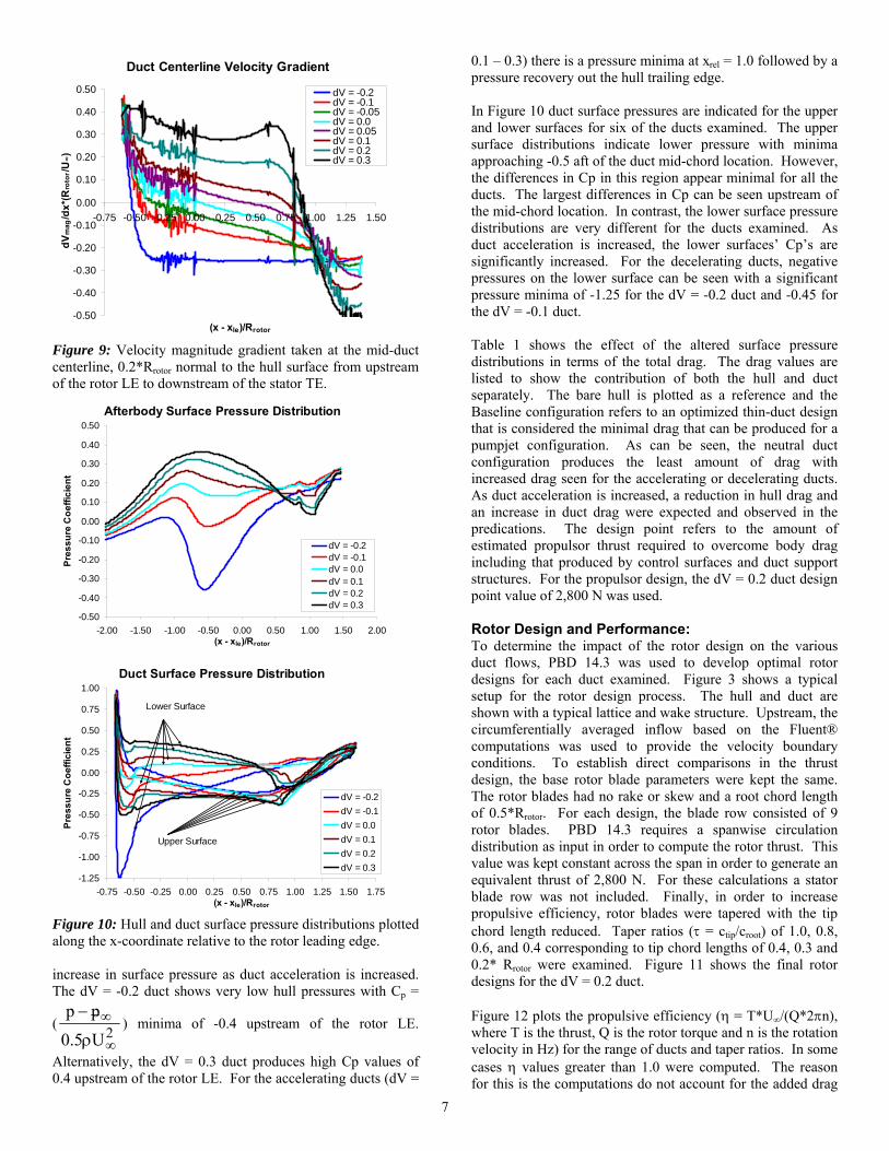
Figure 8: Axial and radial velocity profiles taken at the mid-duct centerline, 0.2*Rrotor normal to the hull surface from upstream of the rotor LE to downstream of the stator TE. the rotor leading edge to the stator trailing edge (TE) (located at xrel = (x – xle)/Rrotor = 0.87). The axial velocities exhibit an approximately linear change in velocity. The modest duct accelerations (dV = -0.1 to 0.1) do not appear as linear. The radial velocity distributions also do not exhibit a linear variation. Figure 9 computes the normalized (by freestream velocity and Rrotor) velocity magnitude gradient in the x-direction obtained by taking the x-derivative of the velocity magnitudes shown in Figure 8. This plot exhibits the effects of a finitely thick boundary layer on the hull and duct in maintaining linear flow acceleration. As can be seen, the acceleration is relatively constant for the dV = -0.2 duct near -0.2. For duct accelerations between -0.1 to 0.2, there appears to be a linear decrease in flow acceleration from upstream of the duct LE to the stator TE. For the dV = 0.3 duct, the acceleration shows a more quadratic behavior with a minimum acceleration of 0.3 0.2*Rrotor downstream of the rotor LE. Hull and duct surface pressure distributions are plotted in Figure 10 with the x-coordinate relative to the rotor LE and normalized by Rrotor. The hull surface pressures exhibit an

6

Duct Centerline Velocity Gradient

-0.50

-0.40

-0.30

-0.20

-0.10

0.00

0.10

0.20

0.30

0.40

0.50

-0.75 -0.50 -0.25 0.00 0.25 0.50 0.75 1.00 1.25 1.50

(x - xle)/Rrotor

dV

mag

/dx

*(R

roto

r/U∞)

dV = -0.2dV = -0.1dV = -0.05dV = 0.0dV = 0.05dV = 0.1dV = 0.2dV = 0.3

Figure 9: Velocity magnitude gradient taken at the mid-duct centerline, 0.2*Rrotor normal to the hull surface from upstream of the rotor LE to downstream of the stator TE.

Afterbody Surface Pressure Distribution

-0.50

-0.40

-0.30

-0.20

-0.10

0.00

0.10

0.20

0.30

0.40

0.50

-2.00 -1.50 -1.00 -0.50 0.00 0.50 1.00 1.50 2.00(x - xle)/Rrotor

Pre

ss

ure

Co

eff

icie

nt

dV = -0.2dV = -0.1dV = 0.0dV = 0.1dV = 0.2dV = 0.3

Duct Surface Pressure Distribution

-1.25

-1.00

-0.75

-0.50

-0.25

0.00

0.25

0.50

0.75

1.00

-0.75 -0.50 -0.25 0.00 0.25 0.50 0.75 1.00 1.25 1.50 1.75(x - xle)/Rrotor

Pre

ssu

re C

oe

ffic

ien

t

dV = -0.2

dV = -0.1

dV = 0.0

dV = 0.1

dV = 0.2

dV = 0.3

Lower Surface

Upper Surface

Figure 10: Hull and duct surface pressure distributions plotted along the x-coordinate relative to the rotor leading edge. increase in surface pressure as duct acceleration is increased. The dV = -0.2 duct shows very low hull pressures with Cp =

(2U5.0

pp

) minima of -0.4 upstream of the rotor LE.

Alternatively, the dV = 0.3 duct produces high Cp values of 0.4 upstream of the rotor LE. For the accelerating ducts (dV =

0.1 – 0.3) there is a pressure minima at xrel = 1.0 followed by a pressure recovery out the hull trailing edge. In Figure 10 duct surface pressures are indicated for the upper and lower surfaces for six of the ducts examined. The upper surface distributions indicate lower pressure with minima approaching -0.5 aft of the duct mid-chord location. However, the differences in Cp in this region appear minimal for all the ducts. The largest differences in Cp can be seen upstream of the mid-chord location. In contrast, the lower surface pressure distributions are very different for the ducts examined. As duct acceleration is increased, the lower surfaces’ Cp’s are significantly increased. For the decelerating ducts, negative pressures on the lower surface can be seen with a significant pressure minima of -1.25 for the dV = -0.2 duct and -0.45 for the dV = -0.1 duct. Table 1 shows the effect of the altered surface pressure distributions in terms of the total drag. The drag values are listed to show the contribution of both the hull and duct separately. The bare hull is plotted as a reference and the Baseline configuration refers to an optimized thin-duct design that is considered the minimal drag that can be produced for a pumpjet configuration. As can be seen, the neutral duct configuration produces the least amount of drag with increased drag seen for the accelerating or decelerating ducts. As duct acceleration is increased, a reduction in hull drag and an increase in duct drag were expected and observed in the predications. The design point refers to the amount of estimated propulsor thrust required to overcome body drag including that produced by control surfaces and duct support structures. For the propulsor design, the dV = 0.2 duct design point value of 2,800 N was used. Rotor Design and Performance: To determine the impact of the rotor design on the various duct flows, PBD 14.3 was used to develop optimal rotor designs for each duct examined. Figure 3 shows a typical setup for the rotor design process. The hull and duct are shown with a typical lattice and wake structure. Upstream, the circumferentially averaged inflow based on the Fluent® computations was used to provide the velocity boundary conditions. To establish direct comparisons in the thrust design, the base rotor blade parameters were kept the same. The rotor blades had no rake or skew and a root chord length of 0.5*Rrotor. For each design, the blade row consisted of 9 rotor blades. PBD 14.3 requires a spanwise circulation distribution as input in order to compute the rotor thrust. This value was kept constant across the span in order to generate an equivalent thrust of 2,800 N. For these calculations a stator blade row was not included. Finally, in order to increase propulsive efficiency, rotor blades were tapered with the tip chord length reduced. Taper ratios ( = ctip/croot) of 1.0, 0.8, 0.6, and 0.4 corresponding to tip chord lengths of 0.4, 0.3 and 0.2* Rrotor were examined. Figure 11 shows the final rotor designs for the dV = 0.2 duct. Figure 12 plots the propulsive efficiency ( = T*U∞/(Q*2n), where T is the thrust, Q is the rotor torque and n is the rotation velocity in Hz) for the range of ducts and taper ratios. In some cases values greater than 1.0 were computed. The reason for this is the computations do not account for the added drag

7

Table 1: Hull and Duct Drag Forces

Hull forces: Drag (N) Hull Drag (N) Duct Drag (N) Total Design Point (N)

Hull Only 1898 427 1898 Baseline Configuration 2152 484 2152 2608

Duct (dV = -0.2) 3807 -1449 2357 2857 Duct (dV = -0.1) 1537 749 2286 2771

Duct (dV = -0.05) 1130 1145 2274 2757 Duct (dV = 0.0) 482 1772 2255 2733

Duct (dV = 0.05) 162 2120 2282 2766 Duct (dV = 0.1) -227 2528 2301 2789 Duct (dV = 0.2) -930 3243 2313 2803 Duct (dV = 0.3) -1517 3879 2363 2864

= 1.0 = 0.8 = 0.6 = 0.4

Figure 11: Rotor blade geometries for the dV = 0.2 duct configuration with taper ratios, , of 1.0, 0.8, 0.6 and 0.4. produced on the hull and duct due to the presence of an operational propulsor, thus artificially inflating the computed efficiency. It is immediately clear that accelerating ducts can significantly increase propulsive efficiency while the decelerating ducts can incur a substantial penalty in terms of performance. This is consistent with previous results as summarized by Carlton [10]. For the present case, the increase in efficiency is quantified. Compared with the neutral duct case, the decelerating duct for dV = -0.2 is 12% less efficient and the accelerating duct for dV = 0.2 is 9% more efficient. For the dV = 0.3 duct, an additional 7% efficiency can be realized at the expense of increased drag. The plot also shows that reduced taper ratio can further increase propulsive efficiency regardless of the duct configuration. For the = 0.4 case, an additional 7% improvement in efficiency was predicted. Optimal Duct and Propulsor Design: Upon initial inspection, it would appear that the propulsor/duct configuration associated with the dV = 0.3 duct would be the best choice. Recall, however, that PUF14.3 only predicts the blade forces and moments, not the induced hull and duct forces. To provide this necessary information, a full 3-D RANS solution of the coupled hull, duct and rotor geometry was performed for selected duct geometries (dV = -0.2, 0.0, 0.1, 0.2 and 0.3). For each rotor design, periodic boundary conditions were applied to compute the total hull, duct and blade forces for a 40 degree wedge (360/9 blades). Next, the

rotor blade was removed and the same problem was computed to provide a bare hull force prediction. In all cases, the RANS test cases were for the rotor blade with tip ratio, = 0.4. The total computed blade thrust as well as the induced drag (defined as the hull and duct drag with an operational propulsor minus the unpropelled case). In these RANS solutions, cases were set up for a bare hull geometry (no rotor), a geometry with an operational rotor alone and another to include the influence of a stator blade row. Periodic boundary conditions were used requiring solution for flow past a single blade only. For these calculations, a momentum source model was implemented in the stator region with a tangential force density sufficient to counteract the torque generated by the rotor thus reducing the total swirl. For these calculations, hull and duct drag as well as rotor thrust were predicted. Predicted hull and duct drag values are plotted separately for cases with and without an operational rotor in Figure 13. This plot illustrates the decrease in hull drag and increase in duct drag with increased duct acceleration. In all cases, the hull drag is increased and duct drag decreased with the operational rotor. All rotors produce thrust primarily in the axial and tangential directions with near zero force produced in the radial direction. This increases the velocity magnitude through the rotor disk thus lowering the pressure on the hull and duct surfaces. As a result, an increase in hull drag and decrease in duct drag (resulting in thrust for most cases) was seen.

8

Prop Efficiency vs. Duct AccelerationPBD 14.3 Computations

0.70

0.75

0.80

0.85

0.90

0.95

1.00

1.05

1.10

1.15

-0.3 -0.2 -0.1 0.0 0.1 0.2 0.3Duct Acceleration

Co

mp

ute

d R

oto

r E

ffic

ien

cy

No Taper

tau = 0.8

tau = 0.6

tau = 0.4

Figure 12: Optimized rotor propulsive efficiency for the range of duct accelerations examined.

Hull and Duct Dragwith and without operational rotor

-3

-2

-1

0

1

2

3

4

dV = -0.2 dV = 0.0 dV = 0.2 dV = 0.3Case

Dra

g/T

des

ign

Dhull/TdesDhull/Tdes (with rotor)Dduct/TdesDduct/Tdes (with rotor)

Figure 13: Hull and duct drag with and without an operational rotor, scaled by the design thrust. Figure 14 also plots the induced hull and duct drag obtained by subtracting the bare hull values for both the rotor solution alone as well as the rotor & stator configuration. As the stator row counteracts the torque generated by the rotor, it also removes the swirl from the flow thus reducing the velocity magnitude. As a result, the overall surface pressures are increased relative to the rotor only case resulting in decreased induced drag forces. The total induced forces are shown in the plot alongside. At this stage, two additional computations are presented. Figure 15 shows the 2-D flow solutions for the baseline, thin duct computations as well as an optimized duct design labeled Duct 12. The previously designed baseline case was shown to be a highly efficient propulsor design and is considered a limiting value for the present IMP design. In the Duct 12 design, the goal was to maximize the flow acceleration into the rotor while minimizing the total induced drag. As can be seen in Figure 15, the flow into the rotor is qualitatively similar to the baseline duct flow. 2-D computations showed the base drag for this duct was 2283 N with a design point of 2767 N. This was only modestly higher than the minimal dV = 0.0 duct values of 2256 N with a 2733 N design point. Table 2 plots the advance coefficient, the base drag, blade thrust and induced drag (normalized by the design thrust) and three propulsive efficiency coefficients. (blade) is the

Induced Hull and Duct Dragwith operational rotor and rotor & stator

-2.5-2

-1.5-1

-0.50

0.51

1.52

2.53

dV = -0.2 dV = 0.0 dV = 0.2 dV = 0.3Case

Dra

g/T

des

ign

Dind(hull)/Tdes (rotor)Dind(hull)/Tdes (rotor&stator)Dind(duct)/Tdes (rotor)Dind(duct)/Tdes (rotor&stator)

Induced Total Dragwith operational rotor and rotor & stator

-0.05

0

0.05

0.1

0.15

0.2

0.25

0.3

0.35

0.4

0.45

dV = -0.2 dV = 0.0 dV = 0.2 dV = 0.3Case

Dra

g/T

des

ign

Dind/Tdes (rotor only)

Dind/Tdes (rotor&stator)

Figure 14: Induced hull and duct drag with and without an operational rotor and rotor & stator combination, scaled by the design thrust. efficiency computed for the blade alone while (eff) accounts for the induced drag effect (=U∞(T – Dind)/(Q*2n) separately for the rotor solution alone as well as the rotor & stator solution. For all cases the computed thrust was kept within 5% of the design thrust. Here, it is clear that the induced drag is reduced for the stator configuration (with slight improvement for the dV = -0.2 duct). The effect of viscosity can clearly be seen as (blade) are on the order of 12% less for the full RANS calculations compared with the potential flow solutions. What is striking, however, is the severe reduction in efficiency due to the induced hull and duct drag for the accelerating ducts for the rotor only solution. While the blade efficiency increases significantly with duct acceleration, the induced drag is also increased as a result reducing the effective efficiency. By adding the stator, the decrease in induced drag provides an increase in effective efficiency. It is interesting that for these cases, there is very little difference in propulsive efficiency for the accelerating ducts. The decelerating duct, however, continues to show decreased efficiency. For design purposes, an increase in efficiency of 1% translates to an effective increase of 1.25% of thrust (assuming propulsive efficiencies of 80%). When accounting for the base drag, it appears that the Duct 12 and ducts with dV = 0.0 and 0.2 are candidates for the optimal configurations. The dV = 0.3 duct has too much base drag to be considered. For these final calculations, a full stator design was performed with results tabulated in Table 3. In these cases, the total drag (base + induced is combined) with the thrust due to the rotor

9

1.25

0.0

0.5

1.0

ux/Uinf

Baseline Duct 12

Figure 15: 2-D RANS solutions of the baseline and Duct 12 cases.

Table 2: Computed Thrust, Induced Drag and rotor efficiency Case Dbase

/Tdesign

T/Tdesign Dind/Tdesign No Stator

Dind/Tdesign -w- Stator

blade only

(eff) no stator

(eff) -w- stator

dV = -0.2 0.923 1.009 0.136 -0.004 0.671 0.581 0.673 dV = 0.0 0.878 0.994 0.216 0.068 0.774 0.606 0.721 dV = 0.1 0.894 0.951 0.245 0.115 0.821 0.610 0.722 dV = 0.2 0.914 0.983 0.299 0.162 0.886 0.617 0.740 dV = 0.3 0.941 1.041 0.406 0.251 0.972 0.593 0.738 Duct 12 0.897 1.025 0.246 0.087 0.801 0.608 0.732 Baseline 0.896 0.958 0.418 0.226 0.943 0.531 0.720

Table 3: Computed drag, thrust, power and rotor efficiency

Case Dbase+Dind/

Tdesign

Trotor

/Tdesign

Tstator

/Tdesign Ttotal - Dtotal Pshaft/Pdesign Peff/Pdesign final

dV = 0.0 0.946 0.994 0.027 0.075 1.073 1.010 0.745dV = 0.2 1.076 0.983 0.020 -0.073 0.929 0.990 0.759Duct 12 0.985 1.025 0.030 0.070 1.070 1.011 0.756

Duct 12 (mod rotor) 1.002 0.987 0.030 0.014 0.992 0.980 0.768Baseline 1.123 0.958 0.125 -0.040 0.849 0.883 0.843

and stator separated out. This was done since the stator can effectively be used to generate thrust as the incoming velocity has a significant swirl component. The total drag is subtracted from the total thrust to provide an indication of the amount of excess or required thrust needed to achieve self-propulsion. The predicted shaft horsepower is then shown with the effective power accounting for the excess/deficit in thrust. The final efficiency accounts for the thrust provided by the stator. As can be seen, the baseline propulsor contains a significant increase in efficiency due to the stator. The optimized stator for this case generates four times the thrust than was possible for the stators optimized for this study. This is likely due to both the increased advance design coefficient, which was significantly higher as well as the fact that the relatively small propulsor diameter allowed for an increase in relative swirl velocity allowing the stator thrust component to be larger. Still, the final propulsor designs appear adequate with efficiencies in excess of 75% seen for these relatively low advance ratios. The Duct 12 case with an improved rotor design was able to meet the power design spec and had the best final efficiency of 76.8%.

Conclusions:

A systematic investigation of a range of duct configurations and associated propulsor designs with applications to integrated motor propulsor design has been presented. The study examined a range of accelerating and decelerating duct configurations and highlighted the associated flow physics. The ducts were designed to incorporate a rim-driven electric motor with sufficient power to propel the vehicle. To provide comparisons, the rotor leading edge tip radius was held constant and various ducts designed to provide constant flow acceleration from upstream of the rotor leading edge to the stator trailing edge. The shape of the duct was dictated by assuming conservation of mass referenced to the rotor leading edge location. The impact of these duct designs on propulsor performance was then studied. The associated rotor designs were optimized for a given duct. Rotors rake and skew parameters were zeroed with chord taper ratio varied to increase rotor performance. Full 3-D RANS solutions were used to specifically isolate the component forces and provide a true indication of propulsor efficiency.

10

2-D RANS solutions highlighted the base fluid dynamics of the various ducts and demonstrated that for constant flow acceleration, the axial flow velocity at the rotor leading edge was decreased with increased duct acceleration. Hull and duct boundary layers were evident in the profiles. Only the dV=-0.2 duct exhibited inflow axial velocities that exceeded freestream velocities. All the other ducts showed axial velocities below freestream. For the dV=0.3 duct, the rotor inflow axial velocities were on the order of half the freestream velocities. The radial velocities at the rotor leading edge had negative mean values on the order of 20% freestream with the profiles showing increased negative velocities at the duct surface for the accelerating ducts with the reverse true for the decelerating ducts. Stator inflow axial velocity profiles were found to be similar for all duct designs as the flow accelerates/decelerates for the different ducts. The radial velocity profiles also showed negative mean values, but appeared to increase in magnitude for the accelerating duct cases. Centerline axial velocity profiles demonstrated approximately constant flow acceleration from the rotor leading edge to the stator trailing edge and were most evident for the extreme duct designs (dV = -0.2 and 0.2-0.3). Velocity gradient data illustrated the effect of the hull and duct boundary layers on the local flow acceleration for the ducts with more modest or zero flow acceleration as there appeared a linear variation in the velocity gradient. In terms of total drag, the neutral duct (dV=0.0) demonstrated the minimum amount of induced drag with increased drag observed for both accelerating and decelerating duct designs. Next, optimized rotor blade designs were produced for each duct using the potential flow blade design code PBD 14.3. The rotor blade efficiencies were increased significantly as duct acceleration was increased and as rotor blade chord taper ratio was reduced. In several instances, the propulsive efficiency of the blade alone was greater than unity. 3-D RANS solutions were used to predict the induced drag component by subtracting the bare hull/duct geometry from the one with the operational rotor. When this was done, a more realistic propulsive efficiency was obtained demonstrating peak efficiencies for the dV=0.2 duct design of 0.617. Even so, there was only a 2% improvement for the dV=0.2 duct compared with the dV=0.0 duct. When an operational stator was factored into the solution, the efficiencies were increased over 25%, demonstrating the importance of the stator. Finally, optimized stator blade rows were designed to provide additional thrust when removing the swirl from the flow. These increased the maximum propulsive efficiencies up to 76%. Interestingly, there was only a 2% difference in propulsive efficiencies between the dV=0.0 and dV=0.2 duct as well as a customized duct that attempted to optimally balance flow acceleration into the rotor and minimize drag. Still, the final propulsor was able to meet the design specification in terms of both thrust and power required with final efficiencies 7% below an optimized, baseline thin duct pumpjet design.

Acknowledgements:

This research was sponsored by the Office of Naval Research under Contract N0001410WX20326, Dr. Scott Hassan

program manager and under Contract N0001410WX20738, Ms. Maria Medeiros program manager.

References:

[1] McCormick, B.W., Eisenhuth, J.J., “Design and Performance of Propellers and Pumpjets for Underwater Propulsion,” AIAA Journal, Vol. 1, No. 10, pp. 2348-2354, 1963. [2] Dang, D.Q., Norrie, D.H., “The Unsteady Pressure Field of a Ducted Impeller,” J. Fluid Mech., Vol. 90, part 2, pp. 209-226, 1979. [3] Zierke, W.C., Straka, W.A., Taylor, P.D., “An Experimental Investigation of the Flow Through an Axial-Flow Pump,” J. Fluids Engr., Vol. 117, pp. 485-409, Sept. 1995. [4] Hughes, M.J., Kinnas, S.A., Kerwin, J.E., “Experimental Validation of a Ducted Propeller Analysis Method,” J. Fluids Engr., Vol. 114, pp. 214-219, June 1992. [5] Lee, Y.T., Hah, C., Loellbach, J., „Flow Analyses in a Single-Stage Propulsion Pump,“ J. Fluids Engr., Vol. 118, pp. 240-248, April 1996. [6] Brockett, T.E., Inviscid Duct-Rotor Interaction Elements for a Decelerating Ducted Propulsor,” Intl. Shipbuild. Prog., Vol. 52, No. 3, pp. 245-271, 2005. [7] Rajagopalan, R.G., Zhaoxing, Z., “Performance and Flow Field of a Ducted Propeller,” Paper No. AIAA-89-2673, AIAA/ASME/SAE/ASEE 25th Joint Propulsion Conference, July 1989. [8] Thurston, S., Amsler, R. C., "Review of Marine Propellers and Ducted Propeller Propulsive Devices," J. of Aircraft, Vol. 3, No. 3, May-June 1966. [9] Morgan, W.G., Caster, E.B., “Comparison of theory and experiment on ducted propellers.” Proc. 7th Symp. Naval Hydrodynamics, Rome, Italy, 1968. [10] Carlton, J. Marine Propellers and Propulsion, Second Edition, Elsevier Publishing, 2007. [11] Huyer, S.A., Fennel, W., Geurtsen, L., Jandron, M., Oliver, S., “Design and Fabrication of the NUWC Light Propulsor,” Proceedings from the Undersea Defence Technology Conference, Europe, Glasgow, Scotland, UK, June 2008. [12] Various Authors, Fluent® Users Guide, Fluent.Inc. [13] Hahn, N.J., Renick, D.H., Taylor, T.E., “PUF-14.4: An Unsteady Analysis Code for Wake-Adapted, Multi-stage Ducted Propulsors,” Massachusetts Institute of Technology Department of Ocean Engineering, December, 2000.

11