WP-2016-024

Integrated Model of Computable General Equilibrium and SocialCost Benefit Analysis of an Indian Oil Refinery: Future Projections

and Macroeconomic Effects

Shovan Ray, A. Ganesh Kumar, Sumana Chaudhuri

Indira Gandhi Institute of Development Research, MumbaiJuly 2016

http://www.igidr.ac.in/pdf/publication/WP-2016-024.pdf

1

Integrated Model of Computable General Equilibrium and Social Cost

Benefit Analysis of an Indian Oil Refinery:

Future Projections and Macroeconomic Effects

Shovan Ray, A Ganesh Kumar and Sumana Chaudhuri,

Indira Gandhi Institute of Development Research (IGIDR)

General Arun Kumar Vaidya Marg

Goregaon (E), Mumbai- 400065, INDIA

Email (corresponding author): shovan@igidr.ac.in

Abstract

Social Cost Benefit Analysis has long been used as a useful tool to appraise and evaluate the

value to a society of a range of investment projects. Various important aspects of this method

have been subject to scrutiny over the decades, such as the appropriate discount rate, whether

the Ramsey Rule of ‘pure time preference’ should be applied as impatience with a positive

rate or zero-rated with concern for future generations; these are important concerns since the

choice of discount rates deeply affect the valuations of future income streams. Other aspects

concerning financial flows and appropriate ‘shadow prices’ have also undergone considerable

attention. However, when a mega-project with the character of a ‘universal intermediate’ is

considered, its multiplier effects may be wide-ranging and permeate several economic and

social layers, and may be captured only in the aggregates. This study, a sequel to a paper that

ignores such macro-aggregative benefits, examines the costs and benefits of Vadinar refinery

in Gujarat with a focus on this welfare dimension on society for the project. The study allows

for this large scale benefit accrual and examines the net economic benefit of refining at

Vadinar by Essar Oil to the region, the state and the country by Social Cost Benefit Analysis.

The framework thus explores a methodological breakthrough in SCBA studies. In

constituting the macroeconomic effects of expansion of the mega oil refinery, the economic

impact is estimated using the Computable General Equilibrium (CGE) model and

incorporated into the cost benefit analysis. This assimilation of CBA with macroeconomic

externality obtained from the CGE model framework is perhaps only one of its kind in

economic analysis of major infrastructure projects of any country. SCBA when combined

with CGE as an analytical tool can be gainfully employed to appraise or evaluate large scale

projects like oil refineries, especially when they make a splash with their mega-sizes as the

Essar Oil refinery is.

Keywords: Social Cost Benefit Analysis, Economic Impact, Computable General

Equilibrium (CGE) Model, Oil Refinery

JEL Code: B41, C51, C52, C53, C54, C55, D50, D58, D60, D61, D62, H23, H43, L71, O22,

Q43

2

1. Introduction

Petroleum, Oil and Lubricants (POL) commands a strategic and critical role in growth

and development. These constitute a major part of energy used in India’s economy, second

only to coal as source of primary energy, and can spur growth in most sectors. India has been

traditionally a net importer of POL products. The country is being forced to spend valuable

foreign exchange to procure additional energy resources. In the recent past, there has been a

growing concern to boost production of petroleum and natural gas from domestic sources as

well as hydrocarbons equity abroad. At present India imports about three-fourths of its crude

requirements. Investing in domestic oil and natural gas exploration is a long-term solution

that will help quench India’s growing energy demands. Since oil and natural gas also play a

critical role in deciding the inflation rate, the prices for these energy commodities have long

been a point of contention in Indian politics. After Government of India allowed private

participation in petroleum refining in India, Essar Oil set up a 9 MMTPA oil refinery at

Vadinar in Gujarat, which started commercial production on May 1, 2008. The current

capacity of the refinery now stands at 20 MMTPA. With state-of-the-art technology, it has

the capability to produce petrol and diesel that meets the latest Euro IV and Euro V emission

standards. The refinery produces LPG, Naphtha, light diesel oil, Aviation Turbine Fuel (ATF)

and kerosene. It has been designed to handle a diverse range of crude — from sweet to sour

and light to heavy. It is supported by an end-to-end infrastructure setup, including SBM

(Single Buoy Mooring), crude oil tanker facility, water intake facilities, a captive power

plant, product jetty and dispatch facilities by both rail and road. To date, Essar Oil’s Vadinar

refinery has successfully processed more than 75 varieties of crude from across the world,

including some of the “toughest crudes”. This comes with an increase in its complexity from

6.1 to 11.8 on the Nelson index, making it India's second largest single-location refinery and

amongst the most complex globally.

In this study, the researchers propose to conduct a study on social cost-benefit

analysis (SCBA) for the Vadinar refinery using up-to-date information to estimate the costs

and benefits associated with the project. The purpose of the study is to briefly examine

whether the commercial refinery project at Vadinar is socially beneficial overall for the

refinery business. The economics of a refinery are complex and depend on many factors.

Profits or losses result primarily from the difference between the cost of inputs and the price

of outputs. In the oil refining business, the cost of inputs (crude oil) and the price of outputs

(refined products) are both highly volatile, influenced by global, regional, and local supply

3

and demand changes. The question of whether the business of refining in aggregate is

socially desirable and economically beneficial is adequate to justify the aggregate cost of

running the refinery. The analysis is done in stages as the effects of a mega-refinery, in fact

any refinery, are wide-ranging as they spill over not just in their local area of activity but

much beyond, extending to the national economy and polity. It is intended that this complex

process is captured in some meaningful way with very high degree of professional norms.

There are however certain effects which may not be amenable to these standards, but we wish

to give pointers to these directions in what follows.

In continuation of Phase I of the study, some important issues were added as fresh

references for Phase II constituting this study. These issues are in two parts. In Phase I the

evaluation was done with data for the period for which output, sales and costs of investment

and operations have been realised/ incurred till date, i.e., 2014-15. This has its clear merit of

basing the evaluation entirely on realised values of the refinery operations. However, the

evaluation of a large and on-going business can be properly made taking into account the

projected useful life of the project, even though there are elements of risks, both anticipated

and unanticipated, going several years into the future. This will constitute one part of the

second phase, further elaborated below. The second part of phase II will incorporate a

completely new element into the evaluation of social benefit costs analysis (SCBA). Since the

Essar Oil Refinery is a large greenfield project which has made a huge impact in the shortage

syndrome that has been the experience of the Indian economy, its macroeconomic

consequences are large - unlike those in many economies such as USA, where a refinery of

similar magnitude would make a lesser impact on the economy in general. In principle it is

like the presence of a large player taking up position rather than a continuum of small players

adding to capacity in the market. This is sought to be captured in the second part of this phase

II under the rubric of the CGE model, which has been developed to capture various

macroeconomic issues at the economy and sectoral levels. These two parts are further

elaborated below.

Projections based Benefit Cost Ratio: Cost-benefit analysis (CBA) is a method of

quantitative economic analysis that is widely used to evaluate existing and proposed projects,

programmes and policies, and which can inform decision-making. CBA is a quantitative

analytical tool to aid decision-makers in the efficient allocation of resources. CBA is also

often used to evaluate the social returns of the use of privately owned resources. In Phase I of

the study, the CBA of EOL’s Vadinar refinery was examined using data available till the

4

current year of operations. Subsequently, input parameters are extended beyond their existing

temporal values. The Economic Net Present Value and Benefit Cost Ratio (BCR) would be

estimated by projecting the Investment Cost, Operating Costs and Revenues, Consumer

Surplus, Producer Surplus, Government Surplus and the Project Externalities using data

received from Essar Oil Limited. This would help in further refinement of the project

deliverables of Phase I of the study and aid in building scenarios for the project CBA.

Assessing macroeconomic impacts using CGE model of Indian economy: CGE models

are useful tools for analysing economy-wide impacts of various economic policies and issues

that have ramifications beyond a particular sector or particular economic agent. Examples

include tax reforms, trade reforms, income distribution policies, energy and environmental

issues, etc.

They are economy-wide models in the sense that they include all sectors of the economy, and

incorporate the behaviour of all economic agents (households, producing sectors,

government, and rest-of-the world). These features make them particularly suited for

analysing issues where the inter-sectoral and inter-agent linkages are very important.

These models are capable of tracking the impacts on prices, output, demand and trade flows

at the individual sector level for all sectors of the economy, as well as impacts on the income,

expenditure and savings of all economic agents in the economy. Since all sectors and all

economic agents are included in the model, they also provide the impacts on several

macroeconomic variables and on the income distribution.

As mentioned earlier, petroleum products being ‘universal’ inputs, any change in the oil

sector will have economy-wide ramifications. Hence, this part of the study will use an

existing CGE model for the Indian economy to assess the impact of an expansion of the

output of refinery sector on the following:

Key macro variables: GDP, exports, imports, exchange rate, consumption, savings,

government fiscal position, investment.

Sectoral impacts: The impacts on sectoral output, prices, demand, export, and import for

both upstream and downstream industries would be covered here. The CGE model includes

all sectors of the economy, viz., agriculture, industry and services, which are categorized into

18 sectors that produce 24 commodity groups. Refinery is one of these 18 sectors, which

5

produces 6 commodity aggregates (LPG, Kerosene, HSD, Motor Spirit, Naphtha, Substitute

fuels such as LDO, Lubes & Tar).

Income distributional impacts: Per capital income of rural and urban households separately

for bottom 30%, middle 40% and top 30%.

Once the second part, constituting the macroeconomic effects of the expansion of oil refinery,

is estimated using the CGE model and interpreted these may be incorporated into the cost

benefit analysis. That part is a novel feature of this exercise. This may be done by identifying

the channels through which they accrue, constituting the macroeconomic externalities of the

refinery project. This exercise will thus provide an added scenario to the assessment made in

phase I of the study which did not have this feature.

2. The Macro externalities of petroleum refineries

These issues of externalities were presented in phase I paper; however in view of their

relevance in the context of the CGE model framework introduced in this study for estimation

of macro benefits and their treatment as macro externalities, this section is included here. The

estimation based on the CGE model framework are monetized and then incorporated in a

later section. Those who may like to get a short summary of what is discussed below may

skip to the recapitulation of these macro externalities later in this section.

The hydrocarbons sector of Indian economy has seen considerable growth for several decades

alongside increased income of its citizens and growth in the national economy. The nature of

this growth has many aspects, and it is useful to highlight them at the outset. Hydrocarbons

form a major part of the total energy sector in India, and with growth in the economy it is a

natural process that energy demand increases, and at a rate determined by the character and

parameters of the energy intensity of growth. If economic growth is energy-intensive it

follows that all subsectors of energy would feel the pressure of demand growth. However,

some subsectors may outpace others, at rates determined by the economic structure. We see

that the Indian economy has not only experienced high energy demand, but also a

considerable shift in demand for hydrocarbons in general and specific petroleum products

(such as diesel and other middle distillates) in particular.

There are two dimensions to this growth profile of energy demand. Oil and natural gas have

not only direct use in specific sectors like transport (motor spirits, diesel, CNG, in

households, industry, etc.) they are also used, very significantly, as ‘universal intermediates’.

Thus petroleum products are not only used in transporting vehicles and firing gas stoves in

6

households, the products of this industry are used as inputs in a variety of activities in a

manner that can be best described as ‘universal intermediates’. Thus natural gas can be used

in power plants as much as coal as inputs, which in turn power several activities in the

economy. Similarly, gas, naphtha and other products of this sector can be used for fertilizers,

along with other multiple uses, and fertilizers are used as inputs in agriculture. Naphtha and

other products can be cracked to derive ethylene, propylene and others, and these in turn can

be used as inputs for producing mono- and poly-products such as polypropylene, with

multiple uses in garments, packaging, plastics, food and several other uses. It is not just that

the products of this industry (oil) are used in specific sectors like transport, but also assume a

more pervading character. Its ramifications are huge and thus its security and stability to the

economy is enormous. With growth in the Indian economy in the sustained manner that has

been recorded for several decades now, it is natural that there is almost an insatiable demand

for the hydrocarbons sector and its various derived products. This has been perceived in

policy circles for some time and has helped in its development in recent decades.

Speaking about the character of the growth process underway, some specific issues such as

the character and speed of urbanization are also important to underline, since this has been

considerable in India. This growth in urban economy is true of all emerging economies in the

world, and included those of the newly industrialized world in Asia and other continents.

With urbanization comes not only considerable growth in urban transport that is frequently

noted, but also other demands made by urban dwellers in procuring supplies from elsewhere

in the country. Thus a variety of industrial products arrive from other cities and industrial

centres, but also agricultural products ranging from common cereals, to fruits and vegetables

and dairy products, grown in the countryside. Hence there is enormous demand on

transportation to move products to urban centres; there is also in turn the increasing demand

arising from agriculture on fertilizers, pesticides and other products of industry to produce

increasing supplies to these centres; and these increase non-linearly in view of increasing

incomes of the urban middle classes. It is these issues that must be kept abreast in

appreciating the enormous pressures on the petroleum sector to fuel the growth in the

economy. What happened in the course of the decades would be easier to comprehend then.

An important point generally missed in the context of inflationary process can be captured in

this context. A balanced and stable production of petroleum products is paramount in this

process of controlled target of inflation. When we measure inflation impacts through metrics

like the wholesale and retail price indices (WPI and CPI) in the economy, it is not simply the

weights of crude and petroleum products in the weighting diagrams of the indices being

7

considered. Through their universal character, these products enter into consumption and

production of most other sectors and add to inflationary pressures through secondary and

tertiary effects. Prices of agriculture could rise, for instance, as a result of its impact, and so

could their transportations to centres of consumption, and also through fertilizer prices

reflected on producer prices. If these prices are not contained, then the subsidy burden to the

exchequer of the large weight of food and fertilizer subsidies spiral, as we have seen in recent

decades; these in turn add to the fiscal deficit burden and hence on the inflationary pressures.

Inflation management is a huge social responsibility of any incumbent government and this in

no small measure is better served by a responsible growth and stability of the hydrocarbons

sector.

India’s food security through rapid strides in the agriculture sector in the last few decades is

well documented. It started in the late 1960s and gathered pace in the 1970s and 1980s, and

sustained with some attendant costs since then. However, it had some distinct characters as it

spread its wings. It was orchestrated through the Green Revolution, which had several

features: it was mainly through increase in yields per acre; it was confined to the principals

cereals, rice and wheat, and later extended to certain crops like maize and sugarcane and

others in select areas; it was confined first to the Indo-Gangetic plains of India and then

spread to coastal peninsular India. For increasing crop yields, common features were the new

technology and seeds that depended on controlled water supply (irrigation), fertilizers and

power, all of which were copiously supplied with heavy subsidy elements built into them.

Petroleum products have made an important contribution in achieving and sustaining that.

India’s much debated green revolution leading to food security would have been a pale

shadow of its success without generous dozes of subsidized inputs, in all of which

hydrocarbons have played important roles, be they irrigation (diesel generated pump sets),

fertilizers and pesticides, tractors, power tillers, harvesters, etc. Food security apart the

income generated in the regions and prosperity of farmers was enormous.

A few other macroeconomic and social effects of the enormous importance of the oil sector

may be quickly listed. India has been deficient in crude petroleum and products in relation to

its net demand for several decades. As a result, there have been large deficits in the external

trade account for imports of crude oil for refining and products for direct consumption to

meet this burgeoning demand. Consequently, the deficit on the foreign exchange account was

ballooning and the external value of the rupee was traditionally under pressure in a controlled

exchange regime. As a result the rupee was considered to be overvalued. This was to a large

extent contributed by the ballooning deficit in the demand supply gap of this sector, and this

8

was considered serious till such time that the economy was liberalised in the early years of

1990s. In fact the critical phase leading to the crisis in the economy in the 1990s and opening

up of the economy soon after and two successive devaluations of the rupee (in 1991) was in

no small measure the reflection of this scenario. With liberalisation and globalisation of the

Indian economy many changes have been wrought, including the controlled regime in the

petroleum sector, the new exploration licensing policy for oil sector (NELP) and the

administered pricing mechanism (APM) that was to be replaced. It is important to note here

that the management of the exchange rate in a controlled regime gives rise to a shadow

exchange rate that may be different from the actual prevailing rate, and thus management of

the oil sector is a task of considerable policy significance. Increased production of crude oil

and refinery products thus add considerably to the benefits accrued to the economy at the

national scale.

There is also pricing and supply chains for petrochemicals as downstream products of

refineries. These influence the growth and locations of downstream products around the

country. For instance, economies around the world with large refining sectors, whether they

are located in the Middle East, Southeast Asia (Singapore), or the United States,

petrochemicals industries have grown in tandem with the growth of refineries, and these add

considerable value chains in the economy with their boosts to output, employment and taxes

in the economy. This has happened in India too with the development of the refining sector

located in different parts of the country. Today the supply of petrochemicals products is so

plentiful that even in rural India with masses of low income households, they have made

pervasive inroads. Even in poor villages and hamlets, a visitor is offered a plastic chairs

which they can afford rather than natural woven materials where they were made to squat.

Several decades back, natural cotton was the apparel of the masses as they could not afford

the synthetics. Today the synthetics fabrics are the apparel of the masses even in rural areas

as they have replaced the natural fibres like cotton, which have become items of luxury at

home, and for exports to markets abroad.

A parallel example may be drawn from automobiles and its linkages with auto-ancillaries,

both growing in lockstep. There are strong case histories of these linkages from around the

world where production takes place; these case histories may be cited from the United States,

Britain, Germany, Japan, and recently from China, South Korea and India. Going a step

backward, the Steel industry has very strong downstream linkages, including the just cited

examples of automobiles and ancillaries. In fact Japan built its giant steel industry even

without the local availability of iron ore; and China’s huge steel capacity is sustained largely

9

by imported ore from India, Australia and several other locations; a similar example is South

Korea, and all these three East Asian economies were dependent on imported ores in varying

proportions. All these industries form a chain of metals-based sector. The story is similar for

refineries and their products, which are petrochemicals. The first is Ferrous-metal-based

value chain, and the refinery chain, whether built on local or imported crude, provide the

petrochemicals value chain. Both these groups, when established provide enormous potential

for value addition, employment and income generation, and direct and indirect tax

collections. This underlines the independent standing of refineries as an engine of growth

even when domestic sourcing of crude oil is limited; when domestic prospecting and

production is added, the chain gets even stronger.

The pricing of petroleum products in the market is another instrument of social policy, quite

apart from the downstream products and pricing of petrochemicals industries discussed

above. It has been noted earlier that these products as universal intermediates, unless properly

managed, have inflationary consequences. There is also social policy of direct subsidy to

consumers in various forms such as kerosene (SKO) subsidy, LPG subsidy and till recently

administered pricing mechanism of motor spirits and diesel. Increase in these prices (or even

their full-cost pricing) can make significant holes in budgets of the poor and the middle

classes, and hence they are sensitive to social and political order in India. It is not just that

income levels matter (through transfers policy of product pricing), which they do, but

inequality among social classes may have consequences on social order. While attempts have

been made for several decades to contain the scale and target beneficiaries of petroleum

subsidies, mainly in the household and agricultural sectors, the magnitudes continue to be

large in scale and inefficient in terms of leakages. These are sensitive issues and government

policies are always alert on them in a democratic set-up.

While in a study of the social costs and benefits of a large refinery it would be important to

capture the ‘shadow price’ of good social order and its stability consequences on the

investment climate for business prosperity, it may be an elusive animal to chase.

Nevertheless, it is worth keeping in mind the importance of social order. It is after all what

makes a lot of difference to the intangible elements that define business confidence. A

volatile climate may not be conducive to the ‘animal spirits’ of entrepreneurs. Hence, even if

this study is unable to measure this element of enormous benefits to the economy and society,

the ‘peace dividend’ may be considered significant.

10

Recapitulation of macro benefits:

It is useful to recapitulate the principal benefits that expansion of the oil sector would bring to

economic welfare and social and political conditions prevalent in India. Stability and

continued growth of this sector is essential to an expanding economy like India where energy

demand has been escalating with economic growth and diversification, intensifying with

global reach and changed lifestyles. It is no longer business-as-usual for the energy sector.

Population growth and rapid urbanization have added fuel to this engine of growth as this

sector is one of the principal contributors to the national energy use. Oil and natural gas

(hydrocarbons) have both direct and intermediate uses for various sectors of the economy,

both as fuel and inputs to these processes. Its universal intermediate character adds weight to

its impact on the national economy. India is sitting on a huge shortage compared with its

burgeoning demand in the face of limited capacity thus far.

Lack of investment over decades in both hydrocarbons prospecting and refining capacity in

the country has resulted in this outcome; both these lines of activity (crude exploration &

production as well as refining capacity) have large gestation lags and risk profiles, especially

in oil and gas prospecting. This has resulted in the economy receiving nightmarish jolts when

caught napping in the face of ballooning demand for products, especially in middle distillates

and overall demand measured in crude throughput. It had several manifestations. Its inflation

consequences and effects on family budgets are significant and these cause social discontents

and disorders which no political system can withstand, let alone a vibrant democracy like

India. Inflation effects of oil price hikes may be measured, but it may be elusive to put

numbers to the ‘multiplier effects’ of an orderly society that provides adequate supply lines

and infrastructure to reach consumers. It is, however, surmised that the effect would be huge

if a metric were to be devised. Analysts believe that a society with discontents may suffer

from business confidence, as being not sanguine to investments and high risk capital; and

these are matters of great consequence as India prospers as a giant world economic power.

The exchange rate effect of oil shortage is a little more subtle conceptually, though quite

large in its result if that could be estimated. The domestic shortage syndrome has two parts,

crude and natural gas availability and the products of refinery. Both shortages would be

reflected in large trade and current account deficits, and have been large and continues to be

so for India. Other than POL, significant contributors to India’s trade deficit are gold and

diamonds & precious stones, though the last group is re-exported largely; gold is not due to

its insatiable demand in India. Refinery products’ shortage increases the net value addition

loss in the imports account, and these add up considerably. Additionally, refineries bring in

11

their downstream products which are also lost in terms of their value additions and multiplier

effects. Imagine a situation where India imported not gold ingots but also all the jewellery

from abroad if there were no jewellers at home. Some powerful examples from steel and

automobiles industries were cited above to drive home the point. The effect of refineries are

similar and additionally all the downstream industries they spawn in different layers. The

current account deficits that translate into BOP deficits put pressure on the exchange rate, and

these could be harmful to domestic consumers, especially for imported goods which become

costlier. A direct consequence, among others, is that imported crude and products in turn

become costlier as they are always denominated in international currencies like the US

dollars. They in turn have inflationary effects discussed above.

It was also emphasized that hydrocarbons are universal intermediates permeating all other

economic activities. Hence, much beyond its inflation, exchange rate and social order

outreach, this source of energy is critical to growth of agriculture, petrochemicals, fertilizers,

power generation and to several others. These downstream industries which develop

alongside refineries support the location and growth of these new activities. To give specific

examples, the proliferation of industries producing plastics, packaging, apparel, among many

other petrochemical products, are now prominent and pervasive even in rural India; it is not

just the frequently cited transport industry that is the beneficiary of this sector. Its growth,

though strenuous over the decades, has fuelled all round development of India. It was pointed

out that refineries spawn other industries which form a chain for petrochemicals This

underlines the independent standing of refineries as an engine of growth even when domestic

sourcing of crude oil is limited; when domestic prospecting and production is added, the

chain gets even stronger.

Furthermore, India’s food security through the much recorded green revolution in the Indo-

Gangetic plains and coastal peninsula would have been a pale shadow of its achievements

without generous dozes of subsidized inputs in all of which hydrocarbons have played

important roles, be they irrigation (diesel generated pump sets), fertilizers, tractors, power

tillers, harvesters, etc. Food security apart, the income generated in the regions and prosperity

of farmers were enormous. Crude oil and natural gas as much as refineries are important cogs

in that wheel of India’s growth. Thus to perceive the economic multiplier effects of this

sector legitimately, we need to consider the total economy for externalities, and not just their

neighbourhoods of activity for ripple effects. These are aggregative and macroeconomic

effects of the sector, which make considerable splash.

12

3. Estimation

3a. Part I: Social Cost Benefit Analysis with Projected Values

Methodology

The noted economists Frank and Bernanke laid CBA as one of the seven core principles of

Economic Sciences. CBA as a tool can be used either to appraise or to evaluate a given

project. Appraisal is done before the commencement of the project and evaluation is done

after the completion of the project. This study focuses on Essar Oil’s already operational

Vadinar Refinery Project. Therefore, technically, this work should be an evaluation of the

project. However, the process of analysis is both retrospective as well as prospective. It is

retrospective in the sense that the project is already completed and it has become fully

operational. It is prospective in the way that by evaluation of the relative merits of the project

in terms of the accrued benefits and costs, it serves as a template for deciding a fresh course

of equity investment in refinery infrastructure augmentation. The study has been informed by

EOL of its new and forthcoming investments and this analysis will aid in appreciation of the

strategic direction of the project as well as its overall fit in the broader socio – economic

rubric.

Formally, the analysis entails solving the following equation:

𝑁𝑆𝐵 = ∑.

𝑛

𝑡=0

(𝑅𝑡 – 𝐶𝑡)/ (1 + 𝑟)𝑡

Where NSB is net social benefit, R is revenues generated from sales of the products, C is the

cost of refining, r is the discount rate, t is the year, and n is the number of years in the project.

The CBA analysis is conducted following generic steps of CBA as described below.

In accordance with the European Commission Guidelines for CBA (2014), the framework of

SCBA is construed for EOL’s Vadinar Refinery. The analysis is based on the following

stages. First, the financial cost and revenue data are converted from financial prices to

accounting or shadow prices by applying explicit conversion factors. Secondly all non-market

impacts have been monetized by the notion of Willingness to Pay (WTP) or Willingness to

Accept (WTA), which are grounded on the concepts of Consumer Surplus (CS) or Producer

Surplus (PS). This, in turn, is expressed quantitatively by the Rule of Half. The process of

determination of CS and PS involves identifying and quantifying the non-monetized costs

and benefit streams associated with the project to generate the specific values of CS and PS.

In the next stage, the externalities of the project are duly incorporated in the analysis. This is

followed by the determination of the Social Discounting Rate for India using the Social Time

Preference Rate (STPR) approach. The final stage involves calculation of economic

performance indicators like ENPV, ERR and the most critical performance criteria for project

evaluation, namely the BCR for the project.

In a separate part of this study discussed below, the macroeconomic effects of this large

infrastructure project are estimated using a computable general equilibrium (CGE) model to

13

capture their effects as part of the larger set of externalities. Those are then integrated in a

separate exercise to arrive at the final picture. That part is a complete innovation of this study,

and as such similar methods are not usually seen in its peer studies.

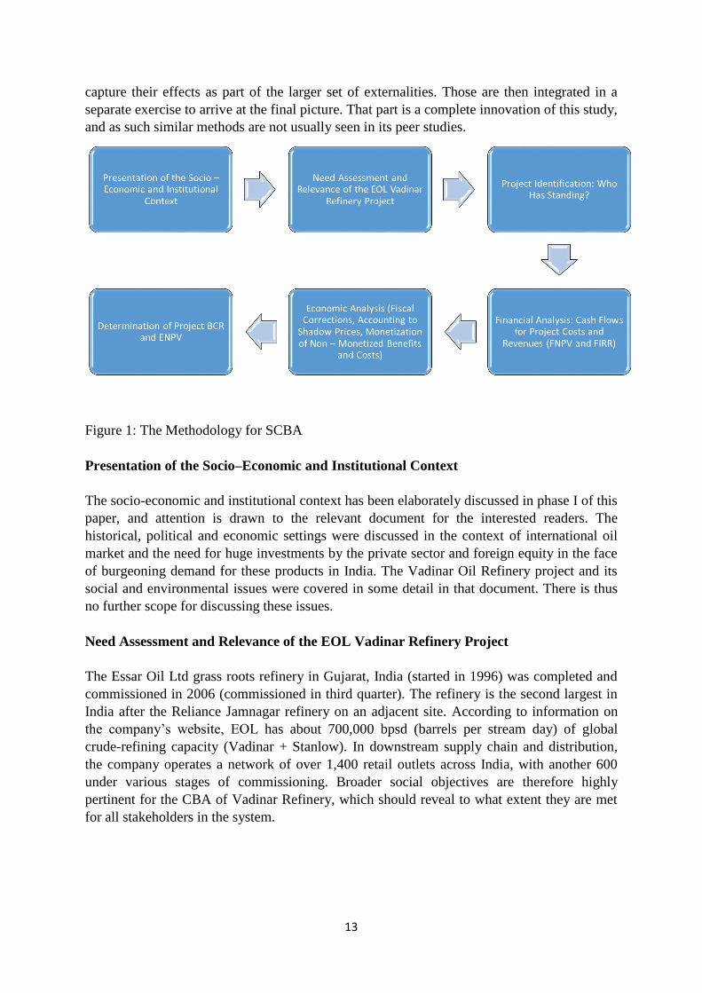
Figure 1: The Methodology for SCBA

Presentation of the Socio–Economic and Institutional Context

The socio-economic and institutional context has been elaborately discussed in phase I of this

paper, and attention is drawn to the relevant document for the interested readers. The

historical, political and economic settings were discussed in the context of international oil

market and the need for huge investments by the private sector and foreign equity in the face

of burgeoning demand for these products in India. The Vadinar Oil Refinery project and its

social and environmental issues were covered in some detail in that document. There is thus

no further scope for discussing these issues.

Need Assessment and Relevance of the EOL Vadinar Refinery Project

The Essar Oil Ltd grass roots refinery in Gujarat, India (started in 1996) was completed and

commissioned in 2006 (commissioned in third quarter). The refinery is the second largest in

India after the Reliance Jamnagar refinery on an adjacent site. According to information on

the company’s website, EOL has about 700,000 bpsd (barrels per stream day) of global

crude-refining capacity (Vadinar + Stanlow). In downstream supply chain and distribution,

the company operates a network of over 1,400 retail outlets across India, with another 600

under various stages of commissioning. Broader social objectives are therefore highly

pertinent for the CBA of Vadinar Refinery, which should reveal to what extent they are met

for all stakeholders in the system.

14

Who has standing?

The boundaries of the analysis should be defined here. The territorial area affected by the oil

refinery project effects is defined as the impact area. This can be of local, as in the Vadinar

region; state or regional as in Gujarat or National in context. A good description of the impact

area requires the identification of the project’s final beneficiaries, i.e. the population that

benefits directly from the petroleum refinery project. These may include, for example, those

identified in the Essar Foundation CSR Paper, papering the benefits of the project that are

accrued by the inhabitants of the larger areas surrounding Vadinar region. The identification

of ‘who has standing’ should account for all the stakeholders who are significantly affected

by the costs and benefits of the project, in accordance to the CBA Guidelines (2014) under

section 2.9.11. This aspect has been adequately reflected in the Micro Externalities analyzed

later in the paper.

Financial Analysis

The financial analysis methodology used in this paper is the Discounted Cash Flow (DCF)

method, in compliance with section III (Method for calculating the discounted net revenue of

operations generating net revenue) of European Commission Delegated Regulation (EU) No

480/2014. The following rules are adopted:

1. Only cash inflows and outflows are considered in the analysis, i.e. depreciation,

reserves, price and technical contingencies and other accounting items which do not

correspond to actual flows are disregarded.

2. An appropriate Financial Discount Rate (FDR) is adopted in order to calculate the

present value of the future cash flows. The financial discount rate reflects the

opportunity cost of capital. In our case, a discount rate of 7.8% is adopted, based on

the long–term annualized interest rate that India’s central bank charges from

commercial, depository banks for loans to meet temporary shortages of funds.

3. Project cash-flow forecasts should ideally be covered for a period appropriate to the

project’s economically useful life and its likely long term impacts. The number of

years for which opex, capex and revenue forecasts are provided should also

correspond to the project’s time horizon (or reference period). The choice of time

horizon affects the appraisal results. In practice, it is therefore helpful to refer to a

standard benchmark, differentiated by sector and based on internationally accepted

practice. The European Commission proposed reference period for the Energy Sector

for 15 years (2015 – 2030) has been considered in this case (ANNEX I to

Commission Delegated Regulation (EU) No 480/2014).

Investment Costs

Investment Cost includes the capital costs of all the fixed assets (e.g. land, constructions

buildings, plant and machinery, equipment, etc.) and non-fixed assets (e.g. start up and

technical costs such as design/planning, project management and technical assistance,

construction supervision, publicity, etc.). In the construction phase, changes in net working

capital (variations in working capital) are also included.

15

The investment cost figures are obtained from the Balance Sheet of EOL, sourced from the

Annual Papers of the company. The costs are shown with a negative sign as they are

considered to be outflows on the part of the operator of the refinery project. The projections

for investment cost are obtained from the company’s internal source and are assumed to be

incremental in nature.

The variations of working capital indicate an investment outlay for the project and are

included as a part of the Total Investment Cost. The Total Investment Cost for the project

works out to be the sum of the total fixed cost, total startup cost and variation in working

capital.

Chart 1: Total Investment Costs

Operating Costs and Revenues

The second step in financial analysis is the calculation of the total operating costs and

revenues. Operating costs include all the costs to operate and maintain (O&M) the plant

operations. Cost forecasts are based on Opex data provided by the company. Although the

actual composition is project-specific, typical O&M costs in the current analyses includes:

cost of raw materials; purchase of traded goods/petroleum products; employee

benefits/expenses/salary costs; operating maintenance; exceptional items; repairs and

maintenance and rent.

The project revenues are defined as the ‘cash inflows directly paid by users for the goods or

services provided by the operation, such as charges borne directly by users for the use of

infrastructure, sale or rent of land or buildings, or payments for services’ (Article 61

(Operations generating net revenue after completion) of (EU) Regulation 1303/2013). The

project revenues till 2014 are obtained from the Annual Papers of EOL and projections from

2015 – 2016 till 2030 are obtained from company’s internal database as provided to the

researchers.

Total Investment Costs

(IN INR CRORES)

2009 2010 2011 2012 2013 2014 2015 2016 2017 2018 2019 2020 2021 2022 2023 2024 2025 2026 2027 2028 2029 2030

Land -59 -80 -3 -4 -6 -4

Buildings -356 -42 -8 -330 -16 -14

Plant & Machinery -12677 -266 -139 -10003 -1208 -653

Office Equipments -35 -9 -6 -6 -1 -3

Furnitures and Fixtures -8 -8 0 -2 -1 -1

Vehicles -8 -1 -1 -2 -1 0

Aircraft 0 -10 0 0 0 0

Total fixed assets (A) -13143 -416 -157 -10347 -1233 -675

Softwares & Licenses -30 -2 -3 -13 -7 -10

Patents 0 0 0 0 0 0

Other pre-production expenses 0 0 0 0 0 0

Consulting Services (for the period, not cumulative acc to EOL main Sheet)-12 -4 -27 -32 -10 -13

Training expenses 0 0 0 0 0 0

R&D expenses 0 0 0 0 0 0

Total start-up costs (B) -42 -6 -30 -45 -17 -23

Train 1 and Train 2 Projected Costs (C ) -250 -250 -250 -8912 -41517 -250 -250 -250 -250 -250 -250 -250 -250 -250 -250 -250

Current Assets (receivables, stocks, cash)

Current Liabilities

Net Working Capital

Variations in Working Capital (D)* -1701 -2288 -3852 -774 -865 -1315

*CWIP including EDC and Adv on Cap A/c

Total investment costs (A) + (B) + (C ) +(D) -14886 -2710 -4039 -11166 -2115 -2013 -250 -250 -250 -8912 -41517 -250 -250 -250 -250 -250 -250 -250 -250 -250 -250 -250

16

Chart 2: Operating Costs and Revenues

Financial Return on Investment

After completion of the tables on Total Investment Costs and Operating Costs and Revenues,

the next step in the financial analysis is to arrive at the Financial Return on Investment. In

order to evaluate the Financial Return, there are two major indicators to be determined:

(a) Financial Net Present Value (FNPV)

(b) Financial Rate of Return (FRR)

The European Guide to CBA (2014) defines Financial Net Present Value as the sum that

results when the expected investment and operating costs of the project (suitably discounted)

are deducted from the discounted value of the expected revenues.

In mathematical notation, FNPV can be expressed as

… (1)

Where St is the balance of cash flow in time t, and at is the financial discount factor chosen

for discounting at time t.

The FNPV is calculated as follows:

… (4)

The calculation of the Financial Return on Investment measures the capacity of the Net

Revenues to remunerate the Net Investment Costs.

Chart 3: Financial Net Present Value of Investment

Operating Costs and Revenues

(IN INR CRORES)

2009 2010 2011 2012 2013 2014 2015 2016 2017 2018 2019 2020 2021 2022 2023 2024 2025 2026 2027 2028 2029 2030

Cost of raw materials consumed -32560 -32856 -42129 -52895 -81334 -88824 -72691 -39352 -54152 -65889 -72258 -143632 -209784 -219964 -232210 -253517 -258055 -271022 -287613 -282029 -286502 -298302

Purchase of traded goods / petroleum products -651 -1706 -1964 -1957 -867 -1276

Employee benefits expense / Salary Cost -97 -98 -120 -135 -186 -225

Other expenses / Operating Expenses -2198 -1090 -1507 -2662 -3387 -4297 -2336 -2442 -2243 -2277 -2552 -4521 -5851 -6180 -6403 -6277 -6625 -6865 -6728 -7098 -7346 -7198

Finance costs -1091 -1181 -1220 -1387 -3424 -3218

Exceptional items -1139 -961 -1083 -1237 -111 0 -2161 -2161 -950 -950 -2400 -2400 -2400 -2400 -2400 -2400 -2400 -2400 -2400 -2400 -2400 -2400

Repairs & Maintenance -32 -58 -47 -119 -121 -127 -280 -280 -316 -316 -316 -316

Rent -15 -10 -11 -17 -20 -23

Total operating costs -37736 -37892 -48023 -60273 -89309 -97840 -77468 -43955.00 -57345.00 -69396.00 -77210.00 -150553.00 -218351.00 -228544.00 -241013.00 -262510.00 -267080.00 -280287.00 -297057.00 -291527.00 -296248.00 -308216.00

Total Operating Revenue 37,700.15 37,376.54 47,342.21 58,761.39 89,186.90 99,472.56 81,337.00 47,491 65,465 78,769 87,516 173,620 248,021 253,652 269,826 293,623 298,464 313,954 333,133 326,830 333,255 347,146

Net operating revenue -35.85 -515.46 -680.79 -1,511.61 -122.10 1,632.56 3,869.00 3,536.00 8,120.00 9,373.00 10,306.00 23,067.00 29,670.00 25,108.00 28,813.00 31,113.00 31,384.00 33,667.00 36,076.00 35,303.00 37,007.00 38,930.00

Evaluation of the Financial Return on Investment (IN INR CRORES)

YEARS

2009 2010 2011 2012 2013 2014 2015 2016 2017 2018 2019 2020 2021 2022 2023 2024 2025 2026 2027 2028 2029 2030

Total operating revenues 37,700.15 37,376.54 47,342.21 58,761.39 89,186.90 99,472.56 81337 47491 65465 78769 87516 173620 248021 253652 269826 293623 298464 313954 333133 326830 333255 347146

Total inflows 37700.15 37376.54 47342.21 58761.39 89186.9 99472.56 81337 47491 65465 78769 87516 173620 248021 253652 269826 293623 298464 313954 333133 326830 333255 347146

Total operating costs -37736 -37892 -48023 -60273 -89309 -97840 -77468 -43955 -57345 -69396 -77210 -150553 -218351 -228544 -241013 -262510 -267080 -280287 -297057 -291527 -296248 -308216

Total investment costs -14886 -2710 -4039 -11166 -2115 -2013 -250 -250 -250 -8912 -41517 -250 -250 -250 -250 -250 -250 -250 -250 -250 -250 -250

Total outflows -52622.00 -40602 -52062 -71439 -91424 -99853 -77718 -44205 -57595 -78308 -118727 -150803 -218601 -228794 -241263 -262760 -267330 -280537 -297307 -291777 -296498 -308466

Net Cash Flow -14921.85 -3225.46 -4719.79 -12677.61 -2237.1 -380.44 3619 3286 7870 461 -31211 22817 29420 24858 28563 30863 31134 33417 35826 35053 36757 38680

IRR 16% (2009-2030) -20%

Discount Rate IRR 83% (2020-2030) Projection Phase

Note: A discount rate of 8.4% has been applied to calculate the valueSensitivity Analysis

Financial Net Present Value of the Investment - FNPV (C) ₹ -31,126.65 2009 - 2014 Time Period IRR

Financial Net Present Value of the Investment - FNPV (C) ₹ 3,014.65 (2020 - 2030) Train 2 2009 - 2015 #NUM!

2009 - 2020 -20%

₹ -1,746.40 (2009-2030) @7.8% 2015 -2020 -26%

2015- 2030 85%

₹ -1,631.27 (2009-2030)@8.4 2009 - 2014 #NUM!

2009 - 2030 16%

Rs. 431.34 2015-2030)@8.4%

Rs. 464.77 (2015-2030@7.8%

17

In our calculation FNPV (C) is -1746.40 INR Crores, by applying a discount factor of 7.8%

for the period 2009 – 2030. It is observed that though the FNPV (C) is negative, the project

breaks even in 2014. The FNPV is negative in the project phase 2009 - 2030 (- INR 1746.40)

as expected, owing to lumpy investments in the Construction Phase. The FNPV (C) turns

positive to INR 3014.65 Crores in the Train – II Phase in 2020 – 2030. The FIRR is 16% for

the project phase 2009 – 2030 and 85% for the projected period 2015 – 2030. A Sensitivity

Analysis is also developed by varying the discount rate and the time horizon for the

discounted cash flows. The FIRR stands at 85% for the projection phase 2015 – 2030. The

PAT , standing at -1180 INR Crores, which was negative in 2013, stood at 126 INR Crores in

2014, in a whopping positive turnaround. The Gross Revenue changed by 10.27% between

2013 and 2014, so did the CP GRM by 0.4% and EBIDTA by 28.8% between 2013 and

2014. It is interesting to observe that Financing Cost has decreased by 6.0%, signaling the

increased efficiency and economies of scale for the refinery.

Economic Analysis

As set out in Article 101 (Information necessary for the approval of a major project) of

Regulation (EU) No 1303/2013, an economic analysis must be carried out to appraise the

project’s contribution to welfare. The economic analysis is distinctly different from the

financial analysis with respect to benefits accrued as a result of the project. Whereas the latter

is merely concerned with the owners or promoters of the project, economic analysis attempts

to identify the project’s impact on the society at large. The key concept is the use of shadow

prices to reflect the social opportunity cost of goods and services, instead of prices observed

in the market, which may be distorted. Sources of market distortions are manifold, like non-

efficient markets, administered tariffs for utilities may fail to reflect the opportunity cost of

inputs due to affordability and equity reasons; and some effects such as no markets (and

prices) are available. The standard approach followed in this paper, consistent with

international practice, is to move from financial to economic analysis. After market price

adjustments and non-market impacts’ estimation, costs and benefits occurring at different

times must be discounted. When market prices do not reflect the opportunity cost of inputs

and outputs, the usual approach is to convert them into shadow prices to be applied to the

items of the financial analysis. The discount rate in the economic analysis of investment

projects, the Social Discount Rate (SDR), reflects the social view on how future benefits and

costs should be valued against present ones. After the use of the appropriate SDR, it is

possible to calculate the project economic performance measured by the following indicators:

Economic Net Present Value (ENPV), and benefit/cost ratio (B/C ratio or BCR).

In economic analysis, for the project inputs, if they are tradable goods, border prices are used.

If they are non-tradable goods, the Standard Conversion Factor (SCF) is used. SCF measures

the average difference between world and domestic prices of a given economy. A set of

conversion factors to the project investment costs and operating costs are applied to convert

the financial costs to economic costs.

Consumer’s Surplus

According to Alfred Marshall (1925), the consumer’s surplus is the maximum sum of money

the consumer would be willing to pay for a given amount of the good, less the amount he

actually pays. The consumers of a refinery project are the oil marketing companies and other

18

agencies who buy the finished products. According to the Annual Paper of EOL for FY 2013

– 14 (page 22), Essar Oil has product off take and infrastructure sharing agreements with all

oil PSUs (the state-owned public sector units). These include Bharat Petroleum Corporation

Ltd. (BPCL), Hindustan Petroleum Corporation Ltd. (HPCL) and the Indian Oil Corporation

Ltd. (IOCL). Essar Oil also offers a wide range of products to bulk customers in the industrial

(cement, power, chemicals, construction, fertilizers, etc.) and transport sectors. Besides, EOL

has also received approvals to supply ATF to the Indian Armed Forces. Essar Oil has an

extensive network of about 1,400 operational retail fuel outlets across the country. EOL also

stands to gain by lowering the cost of fuel supplied to their retail network, by entering into

agreements with various public sector OMCs enabling to source products from their

refineries and depots. This would also result in Opex savings for the company.

Chart 4: Consumer Surplus

Producer Surplus

Estimating the producer surplus, the revenue above the long-run average cost, is an important

part of social cost-benefit analyses of changes in petroleum use. In case of EOL, Producer

Surplus is obtained by learning curve effect, economies of scale and efficient management

practices.

Chart 5: Producer Surplus

Government Surplus

Government has a direct interest in oil consumption because it generates tax revenues. These

revenues can then be used to cut other taxes. However, we first consider these revenues as

accruing to the Government, even though they are likely to be retroceded to consumers over

time. The variation of tax revenues for the government can be calculated with the following

formula. In algebraic form:

∆Φ = T2 Q2 – T1 Q1

Where ∆Φ is the variation in tax revenue. In the case of EOL, we have seen that there is

progressive and substantial increase in tax revenue from 2009 – 2010 onwards.

Chart 6: Government Surplus

Consumer Surplus

2009 2010 2011 2012 2013 2014 2015 2016 2017 2018 2019 2020 2021 2022 2023 2024 2025 2026 2027 2028 2029 2030

HSD

Domestic 5.42 5.1 5.34 4.69 7.82 7.818 6.134 8.6 9.5 8.3 9 10.2 10.4 9.7 10.4 10.4 10 11 11.4 11 12 12.3

Export 0.07 0.34 0.24 0.11 1.1 0.46908 0.36804 1.7 1.6 2.9 1.6 7.6 14 13.9 13.2 14 13.6 12.5 13.1 12.7 11.6 12.1

Total (MMT) 5.49 5.44 5.58 4.8 8.92 8.28708 6.50204 10.3 11.1 11.2 10.6 17.8 24.4 23.6 23.6 24.4 23.6 23.5 24.5 23.7 23.6 24.4

Total (l itre) 6544080000 6484480000 6651360000 5721600000 10632640000 9878199360 7750431680 12277600000 13231200000 13350400000 12635200000 21217600000 29084800000 28131200000 28131200000 29084800000 28131200000 28012000000 29204000000 28250400000 28131200000 29084800000

BAU (INR 49.86/l) 3.26288E+11 3.23316E+11 3.31637E+11 2.85279E+11 5.30143E+11 4.92527E+11 3.86437E+11 6.12161E+11 6.59708E+11 6.65651E+11 6.29991E+11 1.05791E+12 1.45017E+12 1.40262E+12 1.40262E+12 1.45017E+12 1.40262E+12 1.39668E+12 1.45611E+12 1.40856E+12 1.40262E+12 1.45017E+12

Premium 358916611680 355647790080 364800490560 313806873600 583157773440 541779722099 425080175921 673377249600 725678395200 732216038400 692990179200 1163700489600 1595184940800 1542883795200 1542883795200 1595184940800 1542883795200 1536346152000 1601722584000 1549421438400 1542883795200 1595184940800

EOL (@INR 47.4) 3.10189E+11 3.07364E+11 3.15274E+11 2.71204E+11 5.03987E+11 4.68227E+11 3.6737E+11 5.81958E+11 6.27159E+11 6.32809E+11 5.98908E+11 1.00571E+12 1.37862E+12 1.33342E+12 1.33342E+12 1.37862E+12 1.33342E+12 1.32777E+12 1.38427E+12 1.33907E+12 1.33342E+12 1.37862E+12

CS (ROH) FOR HSD 24363609840 24141719040 24763013280 21301516800 39585318720 36776536217 28854857145 45709504800 49259757600 49703539200 47040849600 78993124800 1.08283E+11 1.04732E+11 1.04732E+11 1.08283E+11 1.04732E+11 1.04289E+11 1.08726E+11 1.05176E+11 1.04732E+11 1.08283E+11

CS TOTAL 4060.60164 4023.61984 4127.16888 3550.2528 6597.55312 6129.422703 4809.142857 7618.2508 8209.9596 8283.9232 7840.1416 13165.5208 18047.1184 17455.4096 17455.4096 18047.1184 17455.4096 17381.446 18121.082 17529.3732 17455.4096 18047.1184

PRODUCER SURPLUS 2008 2009 2010 2011 2012 2013 2014 2015 2016 2017 2018 2019 2020 2021 2022 2023 2024 2025 2026 2027 2028 2029 2030

Operating Costs (OC) -28526.46 -29339.86 -37260.8 -46465.7 -68810.88 -75543.7 -60086 -33322.8 -44598.8 -54136.4 -59787.2 -117674 -171279 -179403 -189289 -206436 -210054 -220524 -233893 -229422 -233100 -242632 -308216

Total OR (TOR) 37700.15 37376.54 47342.21 58761.39 89186.9 99472.56 81337 47491 65465 78769 87516 173620 248021 253652 269826 293623 298464 313954 333133 326830 333255 347146 347146

Net Revenue (TOR - OC) 9173.69 8036.68 10081.41 12295.69 20376.02 23928.86 21251 14168.2 20866.2 24632.6 27728.8 55946 76741.72 74248.8 80536.8 87186.92 88410 93430.4 99239.72 97407.6 100155 104513.5 38930

Producers' Surplus 4586.845 4018.34 5040.705 6147.845 10188.01 11964.43 10625.5 7084.1 10433.1 12316.3 13864.4 27973 38370.86 37124.4 40268.4 43593.46 44205 46715.2 49619.86 48703.8 50077.5 52256.76 19465

2008 2009 2010 2011 2012 2013 2014 2015 2016 2017 2018 2019 2020 2021 2022 2023 2024 2025 2026 2027 2028 2029 2030

GS as usual til l 2016, VAT+CST+Excise from 2016 til l 2030 1597.937 6126.371 6975.305 8605.318 6813.153 8359.911 9469.558 10098.8 8770.401 7442 9137 10694 11923 13218 14560 15809 17114 18530 20081 21730 23510 25015 26278

Direct Taxes for the Additional Labour (Indirect); Taxes for Direct and Indirect Labour from 2016 94.21713 97.13106 100.1351 103.2321 106.4248 109.7163 113.1096 174.653 189.7781 600.0649 646.5372 1590.617 1774.993 1992.231 2248.785 2552.392 2912.337 3339.754 3848.003 4453.111 5174.306 6034.657

Sub Total 1597.937 6220.588 7072.436 8705.453 6916.385 8466.336 9579.274 10211.91 8945.054 7631.778 9737.065 11340.54 13513.62 14992.99 16552.23 18057.78 19666.39 21442.34 23420.75 25578 27963.11 30189.31 32312.66

Miscellaneous Taxes* 196.7912 167.8991 214.2154 249.4918 297.2996 329.8458 364.1491 397.2713 432.6606 471.7314 515.2566 562.7161 615.1884 664.1647 710.8785

Total Government Surplus 1597.937 6220.588 7072.436 8705.453 6916.385 8466.336 9579.274 10211.91 9141.845 7799.677 9951.28 11590.03 13810.92 15322.84 16916.38 18455.06 20099.05 21914.07 23936.01 26140.72 28578.3 30853.47 33023.54

*Service Tax, RTO, Road Tax, Municipal Taxes, Mega Insurance Payment

19

Externalities for EOL

For a good Economic Analysis, it is equally important to consider the externalities that are

not accounted for in the converted financial inputs and outputs. While arriving at

externalities, only immediate micro impact of the Essar Oil’s Vadinar Refinery are taken

account of at this stage, namely, indirect employment, mother and child care, education and

livelihood, supply of safe drinking water to the nearby geographies, preventive universal

healthcare, awareness and avoidance of communicable diseases are taken into consideration.

Subsequently, macro externalities accruing to the economy at large are considered as

discussed below.

Chart 7: Externalities for EOL’s Vadinar Refinery

Choice of Social Discount Rate

The Asian Development Bank defines the social discount rate “as a reflection of a society’s

relative valuation on today’s well-being versus well-being in the future.” There is wide

diversity in social discount rates, with developed nations typically applying a lower rate (3–

7%) than developing nations (8–15%).

In our estimate, we have used the Social Time Preference Rate (STPR) Approach to arrive at

the social discount rate for India.

The algebraic expression for the same as expressed by Ramsey formula is as follows:

r = ԑg + p

Where r = Social Discount Rate

ԑ = Elasticity of Marginal Utility with respect to Consumption

g = Growth Rate of Public Expenditure

p = Rate of Pure Time Preference

Applying the values for the variables as above, we have,

r = ((1.64) * (5.3)) + (1.3)

= 9.99% ~ 10%

2008 2009 2010 2011 2012 2013 2014 2015 2016 2017 2018 2019 2020 2021 2022 2023 2024 2025 2026 2027 2028 2029 2030

Indirect Employment 10000 10000 10000 10000 10000 10000 10000 10000 10000 10000 35000 35000 60000 60000 60000 60000 60000 60000 60000 60000 60000 60000 60000

Average Compensation 456953 471085.7 485655.3 500675.6 516160.4 532124.1 548581.6 565548 582514.4 599989.9 617989.6 636529.3 655625.1 675293.9 695552.7 716419.3 737911.9 760049.2 782850.7 806336.2 830526.3 855442.1 881105.4

Impact in Employment 456.95 471.09 485.6553 500.6756 516.1604 532.1241 548.5816 565.548 582.5144 599.9899 2162.963 2227.852 3933.751 4051.763 4173.316 4298.516 4427.471 4560.295 4697.104 4838.017 4983.158 5132.653 5286.632

People Benefitted in Education & Livelihood 15000 15000 15000 15000 15000 15000 15000 15000 15000 15000 15000 15000 15000 15000 15000 15000 15000 15000 15000 15000 15000 15000 15000

EOL Contribution 12768 12768 12768 12768 12768 12768 12768 12768 12768 12768 12768 12768 12768 12768 12768 12768 12768 12768 12768 12768 12768 12768 12768

Impact in Education and Livelihood 19.152 19.152 19.152 19.152 19.152 19.152 19.152 19.152 19.152 19.152 19.152 19.152 19.152 19.152 19.152 19.152 19.152 19.152 19.152 19.152 19.152 19.152 19.152

People benefitted from mother and child healthcare* 260000 260000 260000 260000 260000 260000 260000 260000 260000 260000 260000 260000 260000 260000 260000 260000 260000 260000 260000 260000 260000 260000 260000

EOL Contribution 3897.6927 3897.6927 3897.693 3897.693 3897.693 3897.693 3897.693 3897.693 3897.693 3897.693 3897.693 3897.693 3897.693 3897.693 3897.693 3897.693 3897.693 3897.693 3897.693 3897.693 3897.693 3897.693 3897.693

Impact on healthcare 101.3400102 101.3400102 101.34 101.34 101.34 101.34 101.34 101.34 101.34 101.34 101.34 101.34 101.34 101.34 101.34 101.34 101.34 101.34 101.34 101.34 101.34 101.34 101.34

People benefitted as a result of supply of potable drinking water 10000.00 10000.00 10000.00 10000.00 10000.00 10000.00 10000.00 10000.00 10000.00 10000.00 10000.00 10000.00 10000.00 10000.00 10000.00 10000.00 10000.00 10000.00 10000.00 10000.00 10000.00 10000.00 10000.00

EOL Contribution 21.25 21.25 21.25 21.25 21.25 21.25 21.25 21.25 21.25 21.25 21.25 21.25 21.25 21.25 21.25 21.25 21.25 21.25 21.25 21.25 21.25 21.25 21.25

Impact on drinking water provision 0.02125 0.02125 0.02125 0.02125 0.02125 0.02125 0.02125 0.02125 0.02125 0.02125 0.02125 0.02125 0.02125 0.02125 0.02125 0.02125 0.02125 0.02125 0.02125 0.02125 0.02125 0.02125 0.02125

People benefitted as a result of preventive healthcare 260000 260000 260000 260000 260000 260000 260000 260000 260000 260000 260000 260000 260000 260000 260000 260000 260000 260000 260000 260000 260000 260000 260000

EOL Contribution 1713 1713 1713 1713 1713 1713 1713 1713 1713 1713 1713 1713 1713 1713 1713 1713 1713 1713 1713 1713 1713 1713 1713

Impact on preventive healthcare 44.538 44.538 44.538 44.538 44.538 44.538 44.538 44.538 44.538 44.538 44.538 44.538 44.538 44.538 44.538 44.538 44.538 44.538 44.538 44.538 44.538 44.538 44.538

Total Impact 622.00 636.14 650.71 665.73 681.21 697.18 713.63 730.60 747.57 765.04 2328.01 2392.90 4098.80 4216.81 4338.37 4463.57 4592.52 4725.35 4862.16 5003.07 5148.21 5297.70 5451.68

Reference: http://www.payscale.com/research/IN/Industry=Oil_%26_Gas/Salary for average salary in oil and gas industry in India

http://www.who.int/countries/ind/en/ for per capita health spend in India

http://www.accountabilityindia.in/accountabilityblog/2798-how-much-does-india-spend-elementary-education

http://www.tradingeconomics.com/india/health-expenditure-per-capita-us-dollar-wb-data.html for 61.41 USD per capita spending on health care

*Only Indirect Employment Considered

INR 1105 Bill ion spent on safe drinking water for 1.3 Bill ion til l 10th Five Year Plan people amounting to INR 850

Prinja S, Bahuguna P, Pinto AD, Sharma A, Bharaj G, et al. (2012) The Cost of Universal Health Care in India: A Model Based Estimate. PLoS ONE 7(1): e30362. doi:10.1371/journal.pone.0030362

20

ADB have also recommended SDR for India in the range of 10-12% depending on the

project. A high SDR is usually taken for small projects with immediate benefits. For

megaprojects like oil refineries, a low SDR is preferred, since the benefits are accrued over a

period of time. Thus, our estimate of SDR for India as 10% seems to be reasonably

appropriate.

Once all project cost and benefits have been quantified and valued in money terms, it is

possible to measure the economic performance of the project by calculating the following

indicators.

Economic Net Present Value (ENPV): the difference between the discounted total social

benefits and costs;

B/C Ratio, i.e. the ratio between discounted economic benefits and costs.

The difference between ENPV and FNPV is that the former uses accounting prices or the

opportunity cost of goods and services instead of imperfect market prices, and it includes as

far as possible any social and environmental externalities. This is because the analysis is done

from the point of view of society, not just the project owner. Because externalities and

shadow prices are considered, in our financial analysis, the project though had a negative

FNPV(C), a positive ENPV is recorded in the economic analysis.

The abridged economic analysis is shown below.

Chart 8: Abridged Economic Analysis

A positive ENPV of INR 2, 34,314.98 is obtained for the project phase 2009 – 2030; and

BCR of 3.26 for the period 2009 – 2030 is estimated using the discounted cash flow

technique.

The project is economically sound and financially viable.

In accordance to the the UK Department for Transport (DfT) ‘Value for Money (VfM)

Assessment Guidance’, as laid down in the HM Treasury (2006), the projects are categorized

according to their benefit–cost ratios, adjusted for wider economic impacts. In our case, the

estimated BCR of 3.26, with only micro externalities thus far considered, falls in the category

of “High VfM” in the VfM Assessment criterion; and accordingly refinery projects like these

should be accorded highest priority as they conform to all stipulated guidelines ensuring that

projects are built on a strong economic and commercial case.

ECONOMIC ANALYSIS OF ESSAR OIL

BENEFITS 2008 2009 2010 2011 2012 2013 2014 2015 2016 2017 2018 2019 2020 2021 2022 2023 2024 2025 2026 2027 2028 2029 2030

Total Consumers Surplus 4060.60164 4023.61984 4127.16888 3550.2528 6597.55312 6129.422703 4809.14286 7618.2508 8209.9596 8283.9232 7840.1416 13165.5208 18047.1184 17455.4096 17455.4096 18047.1184 17455.4096 17381.446 18121.082 17529.3732 17455.4096 18047.1184

Total Producers Surplus 4586.845 4018.34 5040.705 6147.845 10188.01 11964.43 10625.5 7084.1 10433.1 12316.3 13864.4 27973 38370.86 37124.4 40268.4 43593.46 44205 46715.2 49619.86 48703.8 50077.5 52256.76 19465

Total Government Surplus 1597.937392 6220.587969 7072.435691 8705.45297 6916.384885 8466.336111 9579.274252 10211.9115 9141.8451 7799.677188 9951.280357 11590.02897 13810.91644 15322.83855 16916.38039 18455.05608 20099.05287 21914.06807 23936.01055 26140.71928 28578.29971 30853.47088 33023.53565

Externalities 622.0043421 636.1369116 650.706571 665.7268383 681.21165 697.1753734 713.6328202 730.59926 747.5657002 765.0411334 2328.014753 2392.903658 4098.802065 4216.814589 4338.367489 4463.566976 4592.522448 4725.346583 4862.155443 5003.068568 5148.209088 5297.703822 5451.683399

Total Benefits 6806.786734 14935.66652 16787.4671 19646.19369 21335.85934 27725.4946 27047.82977 22835.7536 27940.7616 29090.9779 34427.6183 49796.07423 69446.0993 74711.17154 78978.55748 83967.49265 86943.6937 90810.0243 95799.47199 97968.66985 101333.382 105863.3443 75987.33745

Total Investment Costs -11908.8 -14067.2 -17295.2 -19933.6 -20980.8 -21883.2 -7329.6 -7329.6 -7329.6 -7329.6 -33213.6 -200 -200 -200 -200 -200 -200 -200 -200 -200 -200 -200

Total Cost -11908.8 -14067.2 -17295.2 -19933.6 -20980.8 -21883.2 -7329.6 -7329.6 -7329.6 -7329.6 -33213.6 -200 -200 -200 -200 -200 -200 -200 -200 -200 -200 -200

NET BENEFITS 6806.786734 3026.866521 2720.267102 2350.993689 1402.259335 6744.694605 5164.629775 15506.1536 20611.1616 21761.3779 27098.0183 16582.47423 69246.0993 74511.17154 78778.55748 83767.49265 86743.6937 90610.0243 95599.47199 97768.66985 101133.382 105663.3443 75787.33745

BCR (BY NPV METHOD) 3.26 2009-2030 Tax shown above includes EOL, VOTL, VPCL.

ENPV ₹ 234,314.98 2009-2030

BCR (PROJECTED) 10.37 2015-2030

21

The estimated BCR of 10.37 in the projected phase 2015–2030, is in synchronicity with

project guidelines. Improvements in efficiency in Research, Development and Demonstration

(RD&D) in the continuous process plant’s Energy Technologies can achieve a benefit-cost

ratio nearing 15, as outlined by authors Galiana and Sopinka in the Working Paper Series

(2014) published by the Copenhagen Consensus Center in their Energy Assessment Paper for

the Benefits and Costs of the Energy Targets for the Post–2015 Development Agenda. While

the projected phase of 2015-30 provides very optimistic profile of net revenue profile, it

necessarily ignores the negative net revenue phase of such large projects which typically face

a period of losses that cannot be ignored in a proper study of this nature. There is another

aspect that needs consideration.

We consider in what follows the incorporation of macro externalities which span the entire

economy consequent on the establishment of a large project producing goods with their

character as universal intermediates. These effects are then incorporated with the social cost

benefit analysis estimated thus far.

3b. Part II: Computable CGE Model for Economy-wide Effects and Projected Values

Motivation

Capacity expansion in the petroleum refinery sector is likely to unleash several effects that

could be felt across the whole economy. First, there would be increased supply of various

refined products available for end users – both in downstream industries as well as final

consumers. This increase in the supply opens up the possibility of changes in domestic price

of the refined products. For the downstream industries, the increased availability of refined

products along with possible changes in their prices could change their cost of production,

hence their product prices and demand for their products. Thus, those sectors can also witness

an expansion in their output, which in turn can trigger further rounds of output expansion in

all sectors. Besides, they could also have a larger exportable surplus. For the end users of

refinery products (households, government) increased availability and price changes throws

open the possibility that their fuel expenditures could come down, which they can use for

increasing demand for other products and/or savings.

Second, for the refinery upstream industries – crude petroleum, electricity, transport services,

etc., – the expansion of the refinery sector implies additional demand for these inputs. Hence,

they are likely to ramp up their production and/or imports. In the case of crude oil, imports

are likely to increase sharply, which can have an impact on the current account deficit and/or

exchange rate, with attendant consequences for sectoral trade flows.

Third, the expansion of the refinery sector itself, and the induced expansion of other sectors

of the economy would imply an expansion of employment and value added; i.e., gross

domestic product (GDP) in the economy. This additional income would ultimately find its

way to households in the form of wage income and returns to capital. They are likely to

consume a part of this additional income and save the rest. The government too would get a

share of this additional GDP in the form of direct taxes paid by households and production

sectors, indirect tax on the additional demand for various commodities, which in turn is likely

to improve its fiscal position (assuming that the government does not spend it away).

22

Fourth, the additional savings by households and the improvement in the fiscal position of the

government would mean an increase in national savings and hence investment, which in turn

would trigger additional demand for capital goods and hence overall output and GDP in the

economy.

All these multiple channels through which the impacts of an expansion in the refinery sector

are likely to flow have to be properly modelled by carefully capturing the various inter-

sectoral and inter-agent linkages in a consistent manner. One analytical framework that can

capture all such linkages and help in assessing the economy-wide impacts is the computable

general equilibrium (CGE) modeling framework.

The CGE model

CGE models are economy-wide models that have been used widely in India and other

countries to analyse several policy related questions wherein inter-sectoral and inter-agent

linkages are important. In the Indian context, these models have been used to analyse

questions relating to agricultural price policies, energy pricing policies, taxation issues, trade

policies, welfare policies for the poor, etc. They have been used by academic researchers, by

the government (Planning Commission, Ministry of Finance, Ministry of Commerce,

Ministry of Agriculture, etc.), and various international organisation with interest in Indian

economic policies (Australian Centre for International Agricultural Research, Carnegie

Endowment for International Peace, European Union, Food and Agricultural Organisation,

International Development Research Centre of Canada, United Nations Economic and Social

Commission for Asia and the Pacific, United States Department of Agriculture, World Bank,

etc.).

All CGE models have the following characteristics that render them particularly useful for

analysing issues such as the one in focus in this paper.

They include all economic agents, viz., producers (sectors of production), consumers

(households), government, and the rest-of-the-world.

They include all sectors of the economy, viz., agriculture, industry and services, with as

much disaggregation as deemed necessary for analysing the problem at hand.

They characterise the nature of supply, demand, and trade flows in all the goods and

services produced and/or consumed in the economy, taking into account the behavioural

characteristics of producers (who are assumed to maximize profits), consumers (who

maximize utility), and the nature of inter-sectoral flow of goods and services in the

production process.

Production levels and the use of factors of production (labour, capital) are endogenously

determined in the model.

For all goods and services, and also all factors of production (labour, capital), CGE

models solve for the equilibrium supply and demand and the price at which each of these

markets clear; i.e., supply matches demand.

23

They capture the complete flow of all goods and services in a consistent manner; i.e., the

origin of the supply (domestic production / imports) and the end-use (as raw materials,

final consumption, investment including inventory, exports) are explicitly tracked.

Similarly, for factors of production too, they capture the complete flow in terms of the

source of supply (households and/or government that own these factors of production)

and their use in various sectors of the economy.

By capturing the flow of goods and services and factors of production, and the market

clearing prices, these models solve for the income-expenditure accounts for all economic

agents (sectors, households, government, and the rest-of-world) and hence for the nation

as a whole.

Thus, these models capture the macroeconomic effects from microeconomic level; i.e.,

through a bottom-up approach.

This study uses the CGE model of the Indian economy developed by Ganesh-Kumar and

Harak (2015). The model includes 18 sectors (4 agriculture, 10 industrial, 4 services) that

produce 24 commodities (4 agriculture, 16 industrial, 4 services), 2 factors of production, 6

household classes besides the government and the rest-of-world (Table 1).

The present model is built upon a base version of the model developed by Ganesh-Kumar and

Panda (2009) for the Planning Commission. These two models differ on two major counts:

i. The database used by Ganesh-Kumar and Harak (2015) is the social accounting matrix

(SAM) 1 for the year 2011-12, whereas in the case of Ganesh-Kumar and Panda (2009)

the SAM is for the year 2003-04. Further, the level of disaggregation of sectors, goods

and services, factors and household classes also varies between the two SAMs / models.

ii. In terms of model structure, the present model has a more detailed specification of the

energy use in different sectors of the economy. Specifically, a nested production function

approach is adopted wherein every sector’s output is produced by combining raw

materials, energy and factors of production (labour and capital) that generate the value

added (Appendix Figure 1). Energy used in a sector takes into account substitution

possibilities between electrical and non-electrical energy. Further the non-electrical

energy can come from the use of different fuels and the model allows for substitution

possibilities amongst them. In the case of Fertilizers and Chemicals, the nested production

function includes feedstock as an additional requirement and allows for the use of

naphtha and natural gas both as a fuel and also as a feedstock (Appendix Figure 2). For

details see Ganesh-Kumar and Harak (2015).

1 SAM is a matrix representation of the circular flow of income and expenditure in the economy arising out of (a) the buying and selling of goods and services for meeting the production (raw materials), consumption and investment needs of the society and its international trading partners, (b) the buying and selling of factors of production in the course of production process, and (c) financial transfers between agents (taxes, subsidies, foreign remittances, etc.) for which there is no counter-part exchange of goods and services. Thus, the SAM captures the income-expenditure flows of production sectors, households, government and rest-of-world, as well as the supply and demand for various goods and services and factors of production.

24

Table 1: Classifications in the CGE model

Activities (18) Commodities (24) Factors (2) Households (6)

Food crops Food crops Labour Rural - Bottom 30%

Other crops Other crops Capital Rural - 30-70%

Animal products Animal products Rural - Top 30%

Forestry Forestry Urban - Bottom 30%

Coal Coal Urban - 30-70%

Natural gas Natural gas Urban - Top 30%

Crude petroleum Crude petroleum

Other minerals Other minerals

Fertilizers Fertilizers

Chemicals Chemicals

Manufacturing Manufacturing

Construction Construction

Electricity Electricity

Rail transport Rail transport

Road transport Road transport

Other transport Other transport

Other services Other services

Petroleum refining Liquefied Petroleum Gas (LPG),

Kerosene, High Speed Diesel (HSD),

Motor Spirit (MS), Naphtha, Substitute

fuels (SF), Lubes & Tar

Source: Ganesh-Kumar and Harak (2015)

Simulation design and results

In the refinery sector gross refining margin (GRM) can be taken to represent the value

addition in the refinery sector and captures the sector’s contribution to national GDP. A

GRM of 10% is widely construed as a reasonable level representing a long-term average for

the sector. In recent years, the refining sector at the current total refining capacity in the

country of about 200 m.t. across all refiners both private and public accounts for about 1 of

the GDP of the country. This contribution to the national GDP essentially is from the 10%

GRM. These data constitute the base-level around which scenarios are designed to capture

the impact of an expansion in the refinery sector’s capacity. Thus a 20 m.t. entry or expansion

would roughly correspond to a 10% industry capacity expansion. This translates into 1%

additional value addition or GRM as these products have the alternative of being imported

from refineries abroad.

Altogether four scenarios were developed wherein the refinery sector’s output is expanded by

different amounts – 1%, 2.5%, 5%, and 10% – over the base level of 200 m.t. Broadly

speaking, the simulation results indicate that the impacts are proportional at low levels of

output expansion in the refinery sector. But the impacts are somewhat less than proportional

as the magnitude of refinery sector expansion is raised. Considering this and also to maintain

brevity, results for the following two scenarios are presented here:

Scenario-A: This scenario captures the situation where the refinery sector output is

expanded by 1% over a base of 200 m.t.

25

Scenario-B: Here the refinery sector output is expanded by 5% over a base of 200 m. t.

The impacts of the expansion of the refinery sector are assessed at (i) the sectoral level

(Tables 2 and 3) and (ii) macroeconomic, household and government levels (Table 4). At the

sector level, the impacts on domestic prices, domestic demand, exports, domestic output and

imports are assessed. At the macroeconomic level, the variables of interest are the exchange

rage, GDP (aggregate and by broad sectors), aggregate exports and imports, and total

investment in the economy. For households, per capita income across different classes,

household consumption and household savings are examined. The key fiscal variables studied

are direct and indirect tax revenue, total revenue of the government, total expenditure of the

government and government’s dis-savings.2

Expansion of the refinery sector undoubtedly triggers across the board rise in domestic

demand, domestic output and exports for all sectors (Tables 2 and 3). However, the impacts

upon domestic price and imports vary across commodities.

In Scenario A, following the expansion in the refinery sector price of kerosene and motor

spirit alone fall by 0.1% and 0.2%, respectively, while the price of LPG, HSD, naphtha,

substitute fuels and non-substitute fuels rise by 0.2% to 0.9%. In Scenario B, the price

changes are larger than in Scenario A, and additionally the price of HSD also falls by 0.8%.

These price changes give rise to substitution possibilities amongst various fuels setting off

changes in the composition of demand. Further, they also cause a change in per unit cost of

production in all sectors where the refinery products are used, and hence in their respective

product prices with attendant implications for their demand.

The other channel through which the impacts of the expansion of the refinery sector spreads

is through the backward and forward linkages with upstream / downstream industries. The

expansion in the output of these upstream and downstream industries in turn triggers second

round effects that eventually spread through the system.

The net-impact of the price effects and the inter-industry linkage effects is that in Scenario A,

across commodities domestic demand rise between 0.4% for natural gas and 1.8% for coal &

lignite. In Scenario B, it ranges between 1.2% (natural gas) and 6.6% (coal and lignite). Much

of this is on account of a higher rise in raw materials demand, which is higher than demand

by households for final consumption in both scenarios. Thus it is the backward and forward

linkages with upstream / downstream industries of all sectors with all other sectors that drive

overall expansion in domestic demand and hence domestic output.

2 Note that the government dis-saving (i.e., negative savings) is derived from an economic classification of government’s consumption and investment, and closely (but not exactly) corresponds to the combined (Central and States) revenue deficit. For a discussion on this see Planning Commission (2002).

26

Table 2: Sectoral impacts – Scenario A

Commodity Domestic Domestic demand Exports Domestic Imports

price Raw material Household Total

output

Food Crops -0.1 1.1 0.5 0.7 0.4 0.7 -2.3

Plantation, Cash and Other Crops -0.1 1.2 0.8 1.1 0.5 1.1 -0.1

Animal Husbandry and Fishing -0.1 1.2 0.9 1.0 0.4 1.0 -0.9

Forestry -0.3 1.3 0.3 0.8 0.5 0.9 -0.2

Coal and Lignite -0.4 1.7 -0.6 1.8 0.6 2.0 -0.5

Natural Gas 1.7 0.5 -0.7 0.4 0.4 0.3 0.9

Crude Petroleum -0.5 1.0 - 1.1 0.8 3.4 0.8

Other Minerals -0.4 1.2 - 1.1 0.7 2.7 0.5

Fertilizers 0.4 1.0 - 1.0 0.3 1.1 -1.0

Chemicals 0.1 1.3 0.5 1.2 0.5 1.7 -0.8

Manufacturing 0.1 1.2 0.5 0.9 0.5 1.4 -1.2

Construction 0.2 0.9 - 1.1 - 1.1 -

Electricity 0.2 1.2 0.7 1.1 - 1.1 -

Rail Transport 0.0 1.2 1.0 1.1 0.4 1.1 -

Road Transport 0.0 1.1 0.9 1.0 0.4 1.1 -0.8

Other Transport Service 0.0 1.2 0.9 1.0 0.4 1.0 -

Other Services -0.2 1.1 0.7 0.7 0.4 0.8 -1.5

Liquid Petroleum Gas 0.7 1.3 0.8 0.9 0.3 1.0 0.6

Kerosene -0.1 1.1 0.9 0.9 0.4 1.0 -0.7

High Speed Diesel 0.2 1.1 1.1 1.1 0.2 1.0 0.0

Motor Spirit -0.2 1.1 1.2 1.1 0.5 1.0 -0.8

Naphtha 1.5 1.2 - 1.2 0.2 1.0 1.4

Substitute Fuels 0.4 1.0 - 1.0 0.5 1.0 -0.1

Non-Substitutes Fuels 0.9 1.1 0.8 1.0 0.3 1.0 0.6 Source: Author’s estimates using the CGE model discussed above

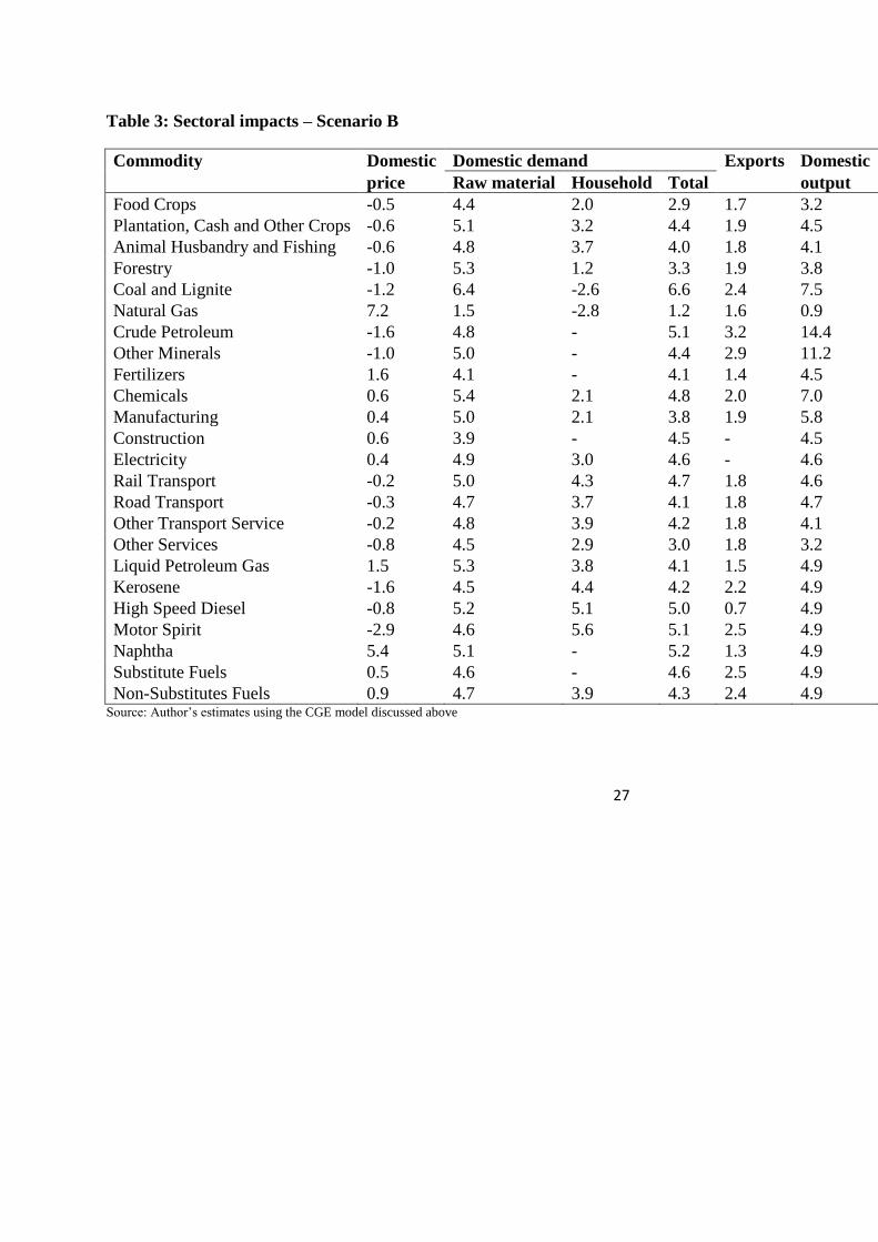
27

Table 3: Sectoral impacts – Scenario B

Commodity Domestic Domestic demand Exports Domestic Imports

price Raw material Household Total

output

Food Crops -0.5 4.4 2.0 2.9 1.7 3.2 -9.4

Plantation, Cash and Other Crops -0.6 5.1 3.2 4.4 1.9 4.5 -0.7

Animal Husbandry and Fishing -0.6 4.8 3.7 4.0 1.8 4.1 -3.9

Forestry -1.0 5.3 1.2 3.3 1.9 3.8 -0.9

Coal and Lignite -1.2 6.4 -2.6 6.6 2.4 7.5 -2.5

Natural Gas 7.2 1.5 -2.8 1.2 1.6 0.9 3.1

Crude Petroleum -1.6 4.8 - 5.1 3.2 14.4 3.8

Other Minerals -1.0 5.0 - 4.4 2.9 11.2 2.2

Fertilizers 1.6 4.1 - 4.1 1.4 4.5 -4.0

Chemicals 0.6 5.4 2.1 4.8 2.0 7.0 -3.1

Manufacturing 0.4 5.0 2.1 3.8 1.9 5.8 -4.8

Construction 0.6 3.9 - 4.5 - 4.5 -

Electricity 0.4 4.9 3.0 4.6 - 4.6 -

Rail Transport -0.2 5.0 4.3 4.7 1.8 4.6 -

Road Transport -0.3 4.7 3.7 4.1 1.8 4.7 -3.6

Other Transport Service -0.2 4.8 3.9 4.2 1.8 4.1 -

Other Services -0.8 4.5 2.9 3.0 1.8 3.2 -5.8

Liquid Petroleum Gas 1.5 5.3 3.8 4.1 1.5 4.9 1.6

Kerosene -1.6 4.5 4.4 4.2 2.2 4.9 -3.9

High Speed Diesel -0.8 5.2 5.1 5.0 0.7 4.9 -1.2

Motor Spirit -2.9 4.6 5.6 5.1 2.5 4.9 -5.2

Naphtha 5.4 5.1 - 5.2 1.3 4.9 5.0

Substitute Fuels 0.5 4.6 - 4.6 2.5 4.9 -1.3

Non-Substitutes Fuels 0.9 4.7 3.9 4.3 2.4 4.9 -0.8 Source: Author’s estimates using the CGE model discussed above

28

Table 4: Macroeconomic, household and fiscal impacts - % change

Variable Scenario A Scenario B

Exchange rate 1.3 5.6

GDP-Total 1.0 4.1

GDP-Agriculture 1.0 4.1

GDP-Industry 1.5 6.2

GDP-Services 0.8 3.5

Total Export 0.4 1.8

Total Import -0.6 -2.4

Total investment 1.3 5.2

Household per capita income

Rural 1 : 0 to 30% 0.5 2.3

Rural 2 : 30% to 70% 0.7 3.2

Rural 3 : 70% to 100% 0.7 3.0

Urban 1 : 0 to 30% 0.6 2.5

Urban 2 : 30% to 70% 0.7 3.0

Urban 3 : 70% to 100% 0.7 2.9

Household consumption (total) 0.7 2.9

Household savings (total) 0.8 3.4

Direct tax revenue 0.7 2.9

Domestic indirect tax revenue 1.1 4.7

Government revenue - Total 0.8 3.1

Government expenditure 0.0 0.4

Government dis-savings -8.9 -30.0 Source: Author’s estimates using the CGE model discussed above

29

Domestic output rises by 0.3% (natural gas) to 3.4% (crude petroleum) in Scenario A while in

Scenario B it ranges between 0.9% (natural gas) and 14.4% (crude petroleum). In many

commodities domestic output expansion exceeds the expansion in domestic demand giving rise

to larger exportable surplus. Consequently exports of all commodities rise, albeit by varying

amounts. Apart from the microeconomic conditions of domestic supply and domestic demand,

exchange rate depreciation3 also acts as a catalyst enabling higher exports.

In several commodities where domestic production can compete effectively with imports such as

agriculture, coal and lignite, fertilizers, chemicals, manufacturing, road transport, and some of

the refinery products, there is a fall in imports (again exchange rate depreciation catalyses this).

However, in commodities such as natural gas, crude petroleum, other minerals and refinery

products such as LPG and non-substitute fuels, the expansion in domestic production is

insufficient to meet the rise in domestic demand and consequently their imports rise

significantly.4

The commodities whose imports rise are those that account for a substantial portion of the total

import bill of the country. Thus the rise in their imports exerts pressure on the current account

balance of the country.5 In these simulations the amount of foreign capital inflows required to

bridge the current account deficit is assumed to remain unchanged, and hence it is the exchange

rate that adjusts to keep the current account in balance. In Scenarios A and B, the Rupee

depreciates by 1.3% and 5.6%, respectively. The depreciating currency acts as a catalyst over

and above the micro-level situation in influencing the changes in sectoral exports and imports.

The sum total of these changes at the sectoral level is that GDP in the country rises by 1% and

4.1% in Scenarios A and B, respectively. Figure 2 shows the impact on GDP at different levels

of expansion of the refinery sector under various scenarios. It is clear, that the GDP impact is

less than proportionate to the expansion in the refinery sector’s output.

The output changes across sectors is such that under both scenarios industrial GDP rises

relatively more than services GDP, while the rise in agricultural GDP is of a similar order as the

rise in overall GDP. The changes in the trade flows are such that overall exports rise in real terms

while imports shrink. Total investment in the economy rises by 1.3% and 5.2%, respectively in

the two scenarios.

At the household level, clearly all households in both rural and urban areas witness a rise in their

per capita income. The rise in per capita income is slightly more for the middle and higher

income groups in both rural and urban areas. With per capital incomes rising all around, total

3 More discussion on the exchange rate follows below.

4 Note that the percent change papered in the tables is over their respective base levels. A given amount of change would imply a larger (smaller) percent change if the corresponding base level is low (high). Thus, for instance, the 3.4% rise in domestic output of crude petroleum is a much smaller amount than the 1.1% rise in its total demand or the 0.8% rise in its imports, both of which are over a larger base.

5 The world price of all commodities is kept constant in these simulations.

30

household consumption rises by 0.7% and 2.9% in Scenarios A and B, respectively. Household

savings too rises in the two scenarios by 0.8% and 3.4%, respectively.6

Figure 2: Impact on GDP at different levels of refinery sector expansion

Source: Author’s estimates using the CGE model discussed above

With household incomes rising, government’s direct tax receipts rise by 0.7% and 2.9% in

Scenarios A and B, respectively. With the domestic demand and domestic output rising across all

sectors, indirect tax collection too rises by 1.1% and 4.7% in the two scenarios. Total revenue7 of

the government in the two scenarios rises by 0.8% and 3.1%, respectively.

In contrast, government’s expenditure remains more or less unchanged in the two scenarios. This

is because in the simulations, it is assumed that all items of government expenditure, viz., current

consumption by government, transfers to households and various subsidies, remain constant in

real terms. As all the expenditure items are decided by government policy, this assumption may

not be too unreasonable. This assumption also helps isolate the pure effects of the refinery

expansion, without any confounding policy changes. The small change observed in government

expenditure largely reflects the change in the nominal expenditure due to price changes.

With government’s revenue rising and its expenditure largely constant, government’s dis-savings

falls significantly by 8.9% and 30% in the two scenarios. That is there is less crowding out of the

total savings by the government. This, along with the rise in household savings seen earlier,

implies that the total savings in the economy rises and allows the investment to rise in the two

scenarios.

6 The model generates income, consumption and savings for each household class. For brevity, only aggregate consumption and savings over all households are papered here.

7 Apart from direct taxes and domestic indirect taxes, the other sources of revenue for the government are customs duty and non-tax revenue consisting of public sector profits and fees largely.

31

CGE Model Exercise: Remarks

The above results are driven by several factors as follows:

The strength of the backward and forward linkages that exist between the refinery sector with

the rest of the economy, in particular and the strength of these linkages amongst other sectors

in general. In the SAM and in the model, the data that determines these linkages are derived

from the Input-Output Table for 2007-08 published by the Central Statistical Office (CSO) of

the Government of India.

The strength of the supply response in various sectors. It is assumed here that there is

sufficient slack capacity in all sectors of the economy, which can be brought to production

fairly quickly. Further, it is assumed that where necessary additional investments are

forthcoming without much friction due to whatever reason.

Behavioural response of households, in terms of their decisions to save or consume, which

items to consume, in what proportions and how much they would substitute various items in

their consumption basket. Household behavioural parameters in the model are derived from

the nation-wide representative surveys on household consumption conducted periodically by

the National Sample Survey Organisation (NSSO) of the Government of India. These are

widely used by academic researchers to characterise various aspects of household behaviour.

Most recent surveys pertaining to the year 2011-12 are used here. It is assumed that the

household behaviour remains stable in the short- to medium-run and hence these behavioural

parameters are held constant in the simulations.

Government policies covering taxes, subsidies, current expenditure, etc., pertaining to all

sectors and all households are kept constant in the present analysis. This was done to isolate

the pure effects of the expansion of the refinery sector. The results obtained could differ were

any of these policies to change.

The current account deficit / foreign capital inflow is kept constant in the analysis here. This

implies that foreign investors do not react in any manner to the expansion of the refinery

sector and the consequent expansion of the economy. If, however, foreign capital inflow

were to rise following the expansion of the economy triggered by the expansion of the

refinery sector, then it could dampen the extent of depreciation of the Rupee. This in turn

could alter the trade flows (both exports and imports) significantly. Such possibility,

however, has not been considered here to keep the analysis simpler.

Keeping these assumptions that are part of the scenario specification, it is clear that expansion of

the refinery sector will have overall positive effects on the economy. In the short to medium-run,

the GDP, household incomes and the fiscal position improves. These effects are expected to

spread through the economy over a period of 5-years. In the long-run, the positive benefits would

32

flow through higher investments that would help keep the growth momentum. Analysis of the

dynamic impacts over several years is, however, beyond scope of this exercise.

4 SCBA with Macro Externality: Integrating CBA with CGE Model

Petroleum products being universal intermediates, they have backward and forward linkages

encompassing the entire national economy. Since the GDP is an aggregative measure of annual

economic activity, it may indicate aggregative welfare in the economy in some very meaningful

sense, and indeed it was the only metric of measuring welfare until recently. Hence, in the

absence of anything superior, this macro indicator of externalities has been used as the metric of

macro externality consequent on the expansion of the refinery sector. As our disaggregated

results show, most of the macro externalities listed in the study are positively impacted. For

instance, all the three major segments, agriculture, industry and services of the economy,

experience expansions. Income, consumption, and savings of both rural and urban households

also increase as a result, and there is virtually no noticeable increase in inequality as the bottom,

middle and higher decile household groups see similar increases in their per capita incomes.

Consequent on these changes, demand and output in the economy have also increased. The

output of fertilizers, chemicals and all critical items of petroleum products, which have

experienced shortage syndrome in the economy, are seen to get the boost in a healthy manner.

Thus we may treat the GDP in this instance as a good metric to represent social welfare and

included in the social benefits of this project.

The analysis in this study has been done using a Computable General Equilibrium (CGE) Model,

as indicated earlier, to capture the effect of an expansion in the refinery sector on the national

economy and its various sectors of activity. In keeping with the investment pattern of Essar Oil

Refinery project, it is spread over three phases of capacity, in 2015 as it exists, and the

installation of Train I and Train II and their staggered coming on stream to full capacity

production.

Further, as mentioned earlier, in recent years, the refining sectors accounts for about 1% of the

GDP of the country. This contribution to the national GDP essentially is from a GRM 10%

(widely construed as a reasonable level representing a long-term average for the sector) and the

current total refining capacity in the country of about 200 m.t.. The simulation exercises are built

around these base-level data to generate their macroeconomic effects.

The model estimates that a 1% increase in the Petroleum Refining capacity of the economy, in

three distinct doses, each dosage leading to a 1% increase in the country’s GDP. For one dosage

this works out to Rs.88,320 crores per annum once the full impact has spread through the

economy. In reality, however, there are lags in the economy implying that it would take some

time for the full impact to be realized. It is assumed that for the full impact to materialize, it is

staggered over 5 years for each dosage. With this assumption the flow of additional GDP due to

the expansion of the refinery sector in three dosages can then be worked out. Table 5 shows the

detailed steps by which the flow of additional GDP is estimated for the three dosages that come

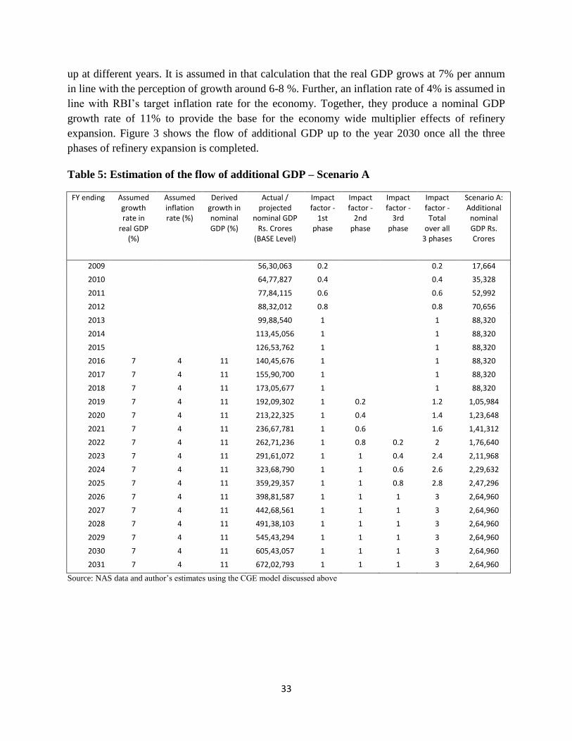
33

up at different years. It is assumed in that calculation that the real GDP grows at 7% per annum

in line with the perception of growth around 6-8 %. Further, an inflation rate of 4% is assumed in

line with RBI’s target inflation rate for the economy. Together, they produce a nominal GDP

growth rate of 11% to provide the base for the economy wide multiplier effects of refinery

expansion. Figure 3 shows the flow of additional GDP up to the year 2030 once all the three

phases of refinery expansion is completed.

Table 5: Estimation of the flow of additional GDP – Scenario A

FY ending Assumed growth rate in

real GDP (%)

Assumed inflation rate (%)

Derived growth in nominal GDP (%)

Actual / projected

nominal GDP Rs. Crores

(BASE Level)

Impact factor -

1st phase

Impact factor -

2nd phase

Impact factor -

3rd phase

Impact factor -

Total over all

3 phases

Scenario A: Additional nominal GDP Rs. Crores

2009 56,30,063 0.2 0.2 17,664

2010 64,77,827 0.4 0.4 35,328

2011 77,84,115 0.6 0.6 52,992

2012 88,32,012 0.8 0.8 70,656

2013 99,88,540 1 1 88,320

2014 113,45,056 1 1 88,320

2015 126,53,762 1 1 88,320

2016 7 4 11 140,45,676 1 1 88,320

2017 7 4 11 155,90,700 1 1 88,320

2018 7 4 11 173,05,677 1 1 88,320

2019 7 4 11 192,09,302 1 0.2 1.2 1,05,984

2020 7 4 11 213,22,325 1 0.4 1.4 1,23,648

2021 7 4 11 236,67,781 1 0.6 1.6 1,41,312

2022 7 4 11 262,71,236 1 0.8 0.2 2 1,76,640

2023 7 4 11 291,61,072 1 1 0.4 2.4 2,11,968

2024 7 4 11 323,68,790 1 1 0.6 2.6 2,29,632

2025 7 4 11 359,29,357 1 1 0.8 2.8 2,47,296

2026 7 4 11 398,81,587 1 1 1 3 2,64,960

2027 7 4 11 442,68,561 1 1 1 3 2,64,960

2028 7 4 11 491,38,103 1 1 1 3 2,64,960

2029 7 4 11 545,43,294 1 1 1 3 2,64,960

2030 7 4 11 605,43,057 1 1 1 3 2,64,960

2031 7 4 11 672,02,793 1 1 1 3 2,64,960

Source: NAS data and author’s estimates using the CGE model discussed above

34

Figure 3: Flow of additional GDP due to a 1% expansion of refinery sector

Source: See Table 5 above for the workings

When this macro externality of CGE is integrated with micro externality of SCBA, it is observed

that 1% rise in nominal GDP due to 1% increase in refinery capacity leads to the increase of

BCR from 3.26 to 11.55 and rise of ENPV from INR 2,34,314.98 crores to INR 10,60,140.37

crores. This result is obtained by factoring the monetized impact of the investment multiplier in

the petroleum-refining sector of the country.

The abridged economic analysis of all perceived surpluses and incorporating both micro and

macro externalities is shown below.

This assimilation of CBA with macroeconomic externality obtained from the CGE model

framework is perhaps a unique endeavor in economic analysis of major infrastructure projects of

any country. Thus the result obtained in this part of the estimation would not have peers to

provide comparison with other infrastructure projects.

ECONOMIC ANALYSIS OF ESSAR OIL

BENEFITS 2008 2009 2010 2011 2012 2013 2014 2015 2016 2017 2018 2019 2020 2021 2022 2023 2024 2025 2026 2027 2028 2029 2030

Total Consumers Surplus 4060.6 4023.6 4127.2 3550.3 6597.6 6129.4 4809.1 7618.251 8209.96 8283.923 7840.142 13165.52 18047.12 17455.41 17455.41 18047.12 17455.41 17381.45 18121.08 17529.37 17455.41 18047.12

Total Producers Surplus 4586.845 4018.3 5040.7 6147.8 10188 11964 10626 7084.1 10433.1 12316.3 13864.4 27973 38370.86 37124.4 40268.4 43593.46 44205 46715.2 49619.86 48703.8 50077.5 52256.76 19465

Total Government Surplus 1597.9374 6220.6 7072.4 8705.5 6916.4 8466.3 9579.3 10212 9141.845 7799.677 9951.28 11590.03 13810.92 15322.84 16916.38 18455.06 20099.05 21914.07 23936.01 26140.72 28578.3 30853.47 33023.54

Micro Externalities (SCBA) 622.00434 636.14 650.71 665.73 681.21 697.18 713.63 730.6 747.5657 765.0411 2328.015 2392.904 4098.802 4216.815 4338.367 4463.567 4592.522 4725.347 4862.155 5003.069 5148.209 5297.704 5451.683

Macro Externalities (CGE) 0 17664 35328 52992 70656 88320 88320 88320 88320 88320 88320 105984 123648 141312 176640 211968 229632 247296 264960 264960 264960 264960 264960

Total Externalities 622.00434 18300 35979 53658 71337 89017 89034 89051 89067.69 89085.16 90648.13 108377 127747 145529 180978.6 216431.9 234224.8 252021.7 269822.5 269963.4 270108.6 270258.1 270412

Total Benefits 6806.7867 32600 52116 72638 91992 116046 115368 111156 116261 117411 122748 155780 193094 216023 255619 295936 316576 338106 360760 362929 366294 370824 340948

Total Investment Costs -11908.8 -14067.2 -17295.2 -19933.6 -20980.8 -21883.2 -7330 -7329.6 -7329.6 -7329.6 -33213.6 -200 -200 -200 -200 -200 -200 -200 -200 -200 -200 -200

Total Cost -11909 -14067 -17295 -19934 -20981 -21883 -7330 -7330 -7330 -7330 -33214 -200 -200 -200 -200 -200 -200 -200 -200 -200 -200 -200

NET BENEFITS 6806.7867 20691 38048 55343 72058 95065 93485 103826 108931 110081 115418 122567 192894 215823 255419 295736 316376 337906 360560 362729 366094 370624 340748

BCR (BY NPV METHOD) 11.55 2009-2030

ENPV ₹ 1,060,140.37 2009-2030

35

Summary and Conclusion

The modeling and simulation for Social Cost Benefit Analysis developed and presented in this

paper is based on the European Commission’s Guide to Cost Benefit Analysis of Investment

Projects: Economic appraisal tool for Cohesion Policy 2014-2020 (European Commission

Directorate General for Regional and Urban policy) authored by Davide Sartori et. al. The work

on SCBA presented here is a unique model developed in the upstream petroleum refining

operations in India. The work takes into account the Investment Cost, Operating Cost, Operating

Revenues to arrive at the Financial Net Present Value of Investment (FNPV) and the Financial

Internal Rate of Return (FIRR). A discount rate of 7.8% is applied in the project phase (2009 –

2030). The FNPV is negative in the project phase 2009 - 2030 (- INR 1746.40) as expected,

owing to lumpy investments in the Construction Phase. The FNPV (C) turns positive to INR

3014.65 Crores in the Train – II Phase in 2020 – 2030. The FIRR is 16% for the project phase

2009 – 2030 and 85% for the projected period 2015 – 2030. A Sensitivity Analysis is also

developed keeping varying the discount rate and the time horizon for the discounted cash flows.

The Consumer Surplus, the Producer Surplus and the Government Surplus is estimated using the

available information obtained from company’s internal database and appropriately projecting

them till 2030 using assumptions grounded on dominant logic for forecasting of income and

expenditures. While arriving at externalities, only immediate micro impact of the Essar Oil’s

Vadinar Refinery, namely, indirect employment, mother and child care, education and

livelihood, supply of safe drinking water to the nearby geographies, preventive universal

healthcare, awareness and avoidance of communicable diseases are majorly taken into

consideration. A positive ENPV of INR 1060140.37 is obtained for the project phase 2009 –

2030; BCR of 3.26 for the period 2009 – 2030 is estimated using discounted cash flow

technique. It moves up to 11.55 when the economy-wide macroeconomic externalities are taken

account of in a CGE framework. The project is thus economically sound and financially viable.

In accordance to the UK Department for Transport (DfT) ‘Value for Money (VfM) Assessment

Guidance’, as laid down in the HM Treasury (2006), the projects are categorized according to

their benefit–cost ratios, adjusted for wider economic impacts. In our case, the estimated BCR of

3.26 with only micro externality into consideration falls in the category of “High VfM” in the

VfM Assessment criterion and accordingly refinery projects like these should be accorded

highest priority as they conform to all stipulated guidelines ensuring that projects are built on a

strong economic and commercial case.

There is abundance of scope to reflect the strategic food and oil security of India from the

macroeconomic perspective; the gradual increase in investor and consumer confidence with

respect to self-reliance in production and consumption of oil and natural gas resources in the

country and the broader social impact of the project, which may be taken up in subsequent

research.

In conclusion, as is observed in this paper, SCBA as an analytical tool can be gainfully employed

to appraise or evaluate large scale projects like Essar Oil’s Refinery at Vadinar, Gujarat. The

SCBA is able to suitably project the holistic societal improvement and enhancement of the

quality of life of all stakeholders, directly or indirectly associated with the project. It is not

36

merely the private costs and benefits, but the overall societal benefits which serves as the guiding

principle for large scale projects like the Essar Oil refinery at Vadinar. The purpose of SCBA is

to facilitate efficient allocation of resources, demonstrating the scope for increased welfare for

society at large.

Acknowledgement

We would like to express our sincere gratitude and heartfelt thanks to Essar Oil Limited for

giving us the opportunity of undertaking this research project on Social and Economic Impact

Analysis of Vadinar Refinery of Essar Oil Limited, which proved to be challenging and

involved. In particular, we are grateful to Mr. Lalit Kumar Gupta, Managing Director and CEO,

Ms. Jaskinder Shingwekar, Vice President (Pricing, Comm., CP), Mr. Deepak Arora, CEO, Essar

Foundation, Mr. Dheeraj Kapoor, Mr. Navdeep Singh and Ms Radhika Agarwal for their helpful

role. We would also like to acknowledge Indira Gandhi Institute of Development Research and

Durgadevi Saraf Institute of Management Studies, Mumbai for providing the scholarly

environment.

37

Reference

Ganesh-Kumar, A. and N. Harak. 2015. “Oil and Natural Gas Price Reforms and its Impacts on

Indian Agriculture”. In S. Mahendra Dev (Ed.) India Development Paper–2015, Oxford

University Press, New Delhi.

Ganesh-Kumar, A. and M. Panda. 2009. “Global Economic Shocks and Indian Policy Response:

An Analysis Using a CGE model”. In K. S. Parikh (Ed.) Macro-Modeling for the Eleventh

Five Year Plan of India, Planning Commission, Government of India / Academic

Foundation, New Delhi.

Planning Commission. 2002. “Paper of the Working Group on Domestic and Foreign Saving for

the Tenth Five Year Plan”, Planning Commission, Government of India, New Delhi.

Asian Development Bank (2011), Economic Analysis, National Grid Improvement Project, RRP

IND 44426 and 44917, accessed from

http://www2.adb.org/Documents/RRPs/IND/44426/44426-014-ind-ea.pdf

Evaluation Unit, DG Regional Policy, European Commission (2014), Guide to Cost-Benefit

Analysis of investment projects: Structural Funds, Cohesion Fund and Instrument for Pre-

Accession, accessed from

http://ec.europa.eu/regional_policy/sources/docgener/studies/pdf/cba_guide.pdf

Chaudhuri, Sumana; Vasigh, Bijan; Chaudhuri, Ranjan, (2015), “Estimation of fair rate of return

on equity for Delhi International Airport,” Journal of Airport Management; Vol. 9 Issue 1,

pp. 76 – 91

Dinara Millington, Rob McWhinney, Zoey Walden (2014), “Refining Bitumen: Costs, Benefits

and Analysis,” Study No. 145, Canadian Energy Research Institute (CERI)

Robert H. Frank and Ben S. Bernanke (2015), Principles of Economics, 5e, McGraw-Hill, ISBN:

0073511404

Alfred Marshall and A C Pigou (1925), “Memorials of Alfred Marshall,” MacMillan, London

UK Department for Transport (DfT) ‘Value for Money (VfM) Assessment Guidance’, (2006),

accessed from

https://www.gov.uk/government/uploads/system/uploads/attachment_data/file/255126/value-for-

money-external.pdf

38

Appendix

Appendix Figure 1: Nested production structure for all sectors other than Fertilizers and

Chemicals

Source: Ganesh-Kumar and Harak (2015)

Appendix Figure 2: Nested production structure for Fertilizers and Chemicals sectors

Source: Ganesh-Kumar and Harak (2015)

39

Appendix 3

Comparison of CBAs across Sectors (Nationally and Internationally)

A comparative analysis of the Vadinar Refinery is also made with other National

and International transportation and infrastructural projects.

Table A: Comparative Analysis of National Projects

It may be mentioned here that for Delhi International Airport Limited the BCR was

estimated to be 3.78 (Chaudhuri, Vasigh, Chaudhuri, 2015)

Table B: Comparative BCRs for Selected International Transportation

Projects

In case of CVISN Program life-cycle benefit/cost analysis is conducted taking into

account the long term social benefits associated with the project.

Project Location BCR

Commercial Vehicle Information Systems and Networks

(CVISN) Program (1)

Maryland and

Virginia 12.5

Truck Bypass (6 Miles) Interstate 205 (I-205) Mountain

House Parkway Interchange in San Joaquin County to a

point west of the Interstate 580 (I-580) Grant Line Road

Interchange in Alameda County, California Department

of Transportation (Caltrans) (2) California 1.3

Monorail (3) Washington 1.23

Public Transport: public transport telematics system

incorporating real-time passenger information, bus and

train priorities at traffic signals, and schedule monitoring

(4) Helsinki, Finland 3.3

Rock County Airport Runway (5) Wisconsin 4.9

TRANSPORTATION BENEFIT COST ANALYSIS

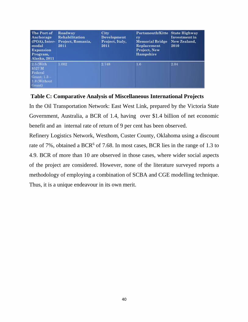
40

Table C: Comparative Analysis of Miscellaneous International Projects

In the Oil Transportation Network: East West Link, prepared by the Victoria State

Government, Australia, a BCR of 1.4, having over $1.4 billion of net economic

benefit and an internal rate of return of 9 per cent has been observed.

Refinery Logistics Network, Westhom, Custer County, Oklahoma using a discount

rate of 7%, obtained a BCR6 of 7.68. In most cases, BCR lies in the range of 1.3 to

4.9. BCR of more than 10 are observed in those cases, where wider social aspects

of the project are considered. However, none of the literature surveyed reports a

methodology of employing a combination of SCBA and CGE modelling technique.

Thus, it is a unique endeavour in its own merit.