Integer Maximum Flow in WirelessSensor Networks with EnergyConstraint

Hans L. Bodlaender

Richard B. Tan

Thomas C. van Dijk

Jan van Leeuwen

Technical Report UU-CS-2008-005

Februari 2008

Department of Information and Computing Sciences

Utrecht University, Utrecht, The Netherlands

www.cs.uu.nl

ISSN: 0924-3275

Department of Information and Computing Sciences

Utrecht University

P.O. Box 80.089

3508 TB UtrechtThe Netherlands

Integer Maximum Flow in Wireless Sensor

Networks with Energy Constraint ?

Hans L. Bodlaender a,1 Richard B. Tan a,b

Thomas C. van Dijk a and Jan van Leeuwen a

aDepartment of Information and Computing SciencesUtrecht University

Utrecht, The Netherlandshansb,rbtan,thomasd,jan@cs.uu.nl

bDepartment of Computer ScienceUniversity of Sciences & Arts of Oklahoma

Chickasha, OK, U.S.A.

Abstract

We study the integer maximum flow problem on wireless sensor networks with en-ergy constraint. In this problem, sensor nodes gather data and then relay them to abase station, before they run out of battery power. Packets are considered as inte-gral units and not splittable. The problem is to find the maximum data flow in thesensor network subject to the energy constraint of the sensors. We show that thisintegral version of the problem is strongly NP-complete and in fact APX-hard. It fol-lows that the problem is unlikely to have a polynomial time approximation scheme.Even when restricted to graphs with concrete geometrically defined connectivityand transmission costs, the problem is still strongly NP-complete. We provide someinteresting polynomial time algorithms that give good approximations for the gen-eral case nonetheless. For networks with bounded treewidth greater than two, weshow that the problem is weakly NP-complete and provide pseudo-polynomial timealgorithms. For a special case of graphs with treewidth two, we give a polynomialtime algorithm.

? This work was supported by BSIK grant 03018 (BRICKS: Basic Research inInformatics for Creating the Knowledge Society).1 Corresponding author.

1 Introduction

A wireless sensor (or smart dust) is a small physical device that containsa microchip with a miniature battery, and a transmit/receive capability oflimited range. Sensors have been deployed in different environments to gatherdata, perform surveillances and monitor situations in diverse areas such asmilitary, medical, traffic and natural environments. (See e.g. Zhao and Guibas[21].)

As the battery power of a sensor is limited and non-replaceable, it is crucial tomaximize the lifetime of the wireless sensor network to ensure the continuingfunction of the whole network. We study the situation of a data-gatheringsensor network, where sensors are deployed in the field to gather data andthen relay the data packets via other sensors back to a base station. It isdesirable to get as many data packets as possible from the source sensors tothe base station, before some of the sensor batteries are depleted. This thenbecomes an instance of the maximum flow problem, subject to the energyconstraint of the lasting battery power of each sensor.

Most of the research papers for the maximum flow problem with energy con-straint on wireless sensor networks (e.g. [8,9,12,16–18,20]) cast the probleminto a Linear Programming (LP) form and assume fractional flows, i.e., split-ting of packets into fractional portions is allowed. The corresponding LP-formulations then have polynomial time algorithms. These papers then presentseveral heuristics that speed up the algorithms and compare various simulationresults. A few papers [8,12,16,17] modified the Polynomial Time Approxima-tion Scheme (PTAS) of Garg and Konemann [14] to obtain fast approximationalgorithms.

As data packets are usually quite small, there are situations where splittingof packets into fractional ones is not desirable nor practical. We consider amodel where data packets are considered as units that cannot be split, i.e.the packet flows are of integral values only. We call this the Integer MaximumFlow problem for Wireless Sensor Network with Energy Constraint: the Inte-ger Max-Flow WSNC problem. The corresponding LP formulation becomesInteger Programming (IP) and may no longer have a polynomial time solution.

We show that the problem is in fact strongly NP-complete, and thus unlikely tohave a Fully Polynomial Time Approximation Scheme (FPTAS) or a pseudo-polynomial time algorithm, unless P=NP. This result also holds for a class ofgraphs with geometrically defined connectivity and transmission costs, evenwhen the nodes lie on a line. Furthermore, we show that even for a specialfixed range model, the problem is APX-hard, thus unlikely to have even aPTAS (unless P=NP). We also provide some approximation algorithms for

4

the problem that do give good approximations nonetheless.

Many hard problems have polynomial time solutions when restricted to net-works with bounded treewidth (see e.g. [4]). However, we show that for net-works with bounded treewidth greater than two, the Integer Max-Flow WSNCproblem is weakly NP-complete. We provide pseudo-polynomial time algo-rithms to compute integer maximum flows in this case. For a special caseof graphs that have treewidth two, namely those graphs that have treewidthtwo when we add an edge from the single source to the sink, we provide apolynomial time algorithm.

The paper is organized as follows. In Section 2, we describe the model and theproblem in detail. Section 3 covers the complexity issues. We show here thevarious NP-completeness results and describe some approximation algorithms.Section 4 contains the results for networks with bounded treewidth.

2 Preliminaries

In this section, we discuss the model we use and the precise formulation ofthe Integer Max-Flow WSNC problem. We also discuss some variants of theproblem, and give some definitions used in other sections.

2.1 The Model

Our model of a sensor is based on the first order radio model of Heinzelmanet al. [15]. A sensor node has limited battery power that is not replenishable.It consumes an amount of energy εelec = 50nJ/bit to run the receiving andtransmitting circuitry and εamp = 100pJ/bit/m2 for the transmitter amplifier.In order to receive a k-bit data packet, a sensor has to expend εelec · k energy,while to transmit the same packet from sensor i to sensor j will cost εelec · k +εamp · k · d2

ij energy, where dij is the distance between sensors i and j.

We model a wireless sensor network as a directed graph G = (N, A), whereN = 1, 2, . . . , n∪t are the n sensor nodes along with a special non-sensorsink node t, and A is the set of directed arcs ij connecting node i to nodej, i, j ∈ N . A sensor node i has energy capacity Ei and each arc ij has costeij, the energy cost of receiving (possibly from some node) a packet and thentransmitting it from node i to node j. We assume that no data is held backin intermediate nodes 6= t, i.e., data that flows in will flow out again, subjectto the battery constraint of these nodes. All Ei’s and eij’s are non-negativeinteger values.

5

The general model assumes that each sensor can adjust its power range foreach transmission. We also consider in the next section the fixed range model,where each sensor has only a few fixed power settings. All our graphs areassumed to be connected. For each arc ij ∈ A, there is a directed path from asource node to the sink node that uses this arc.

2.2 The Problem

Given a wireless sensor network G, there is a set S of source sensor nodes,used for gathering data. The sink node t is a base station and is equipped withelectricity and thus has unlimited energy to receive all packets. The remainingnodes are just relaying nodes, used to transfer data packets from the sourcenodes to the sink node. One would like to transmit as many packets as possiblefrom the source nodes to the sink node. This is feasible as long as the batterypower in the network suffices to do so. The transmission process can be viewedas a flow of packets from the sources to the sink. The problem is then to findthe maximum flow of data packets in the network subject to the battery powerconstraint.

We assume that the data packets are quite small, thus it is neither reasonablenor practical to split them further into fractional portions. A flow fij is a func-tion that assigns to each arc ij a non-negative integer value. This correspondsto the number of packets being sent via the arc ij. A flow is a feasible flow if∑

j fij · eij ≤ Ei for all nodes i ∈ N , where the sum is taken over all j withij ∈ A; i.e., the flow through a node cannot exceed the battery capacity ofthe node.

We can now formulate the maximum flow problem for wireless sensor networksas the problem of determining the maximum number of packets that can bereceived by the sink node. We call this problem the Integer Maximum Flowproblem for Wireless Sensor Networks with energy Constraints or Integer Max-Flow WSNC problem for short. The problem has the following Integer LinearProgramming formulation.

6

The Integer Max-Flow WSNC problem:Objective: maximize F =

∑j∈N fjt, t is the sink node,

subject to the following constraints:

fij integer, ∀ij ∈ A (1)

fij ≥ 0, ∀ij ∈ A (2)∑j∈N

fij =∑j∈N

fji, ∀i ∈ N − S − t (3)

∑j∈N

fij · eij ≤ Ei, ∀i ∈ N (4)

Condition (3) is the conservation of flow constraint. It simply states that withthe exception of the source and sink nodes, every node must send along thepackets that it has received. Condition (4) is the energy constraint for thefeasible flow: the energy needed to (receive and) transmit packets must bewithin the capacity of the battery power of each node. This condition alsodistinguishes the (integer) max-flow WSNC problem from the standard max-flow problem: there, the constraint condition is just fij ≤ cij, where cij is theflow capacity of arc ij.

We note that without loss of generality, we can augment the network with asuper source node s with unlimited energy to send and connect it to all thesource nodes with some fixed cost. We can then view the network as having asingle source and a single sink with a single commodity, subject to the batteryenergy constraint. However, note this may affect the treewidth of the network;the results for networks of bounded treewidth in section 4.1 assume a singlesource.

2.3 Other Variants

Other variants of the problem formulation exist for wireless sensor networkswith energy constraint. For example, Floreen et al. [12] use the following energyconstraint in their LP-formulation of the problem:∑

j∈N

τij · fij +∑j∈N

ρ · fij ≤ Ei, ∀i ∈ N,

where the parameters τij is the energy expended in sending a packet from nodei to node j and ρ is the corresponding energy for receiving a packet. Theirobjective function in the LP-formulation is also slightly different and has someextra parameters that are non-integral.

Chang and Tassiulas [9] give an LP-formulation similar to ours for the sin-gle commodity case, except they formulate the problem over the set of all

7

paths from s to t and allow fractional packets. They also consider the multi-commodity case.

2.4 Definition of Treewidth

We define the concept of treewidth for a general (undirected) graph Gu. Thisconcept is used in Section 4.

Definition 1 A tree-decomposition of a graph Gu = (N, Au) is a pair D =(X,T ) with T = (P, F ) a tree and X = Xp | p ∈ P a family of subsets ofN , one for each node of T , such that

• ⋃p∈P Xp = N ,

• for every edge i, j ∈ Au, there exists a p ∈ P with i ∈ Xp and j ∈ Xp,• for all p, q, r ∈ P : if q is on the path from p to r in T , then Xp ∩Xr ⊆ Xq.

The treewidth of a tree-decomposition (Xp | p ∈ P, T = (P, F )) is maxp∈P |Xp| − 1.The treewidth of a graph Gu is the minimum treewidth over all possible tree-decompositions of Gu.

An undirected graph Gu = (N, Au) is said to be a minor of a graph Hu =(M, Bu), if Gu can be obtained from Hu by a series of vertex deletions, edgedeletions, and edge contractions; where an edge contraction is the operationthat takes two adjacent vertices i and j, and replaces it by a new vertex,adjacent to all vertices that were adjacent to i or j. It is well known that thetreewidth does not increase when taking minors.

In this paper, the treewidth of a directed graph G is just the treewidth of theunderlying undirected graph Gu, i.e., the graph obtained by dropping directionof edges.

3 Complexity

We will first look at the complexity of the problem on general graphs witharbitrary costs at the arcs. We show the problem is NP-complete. Next we showthis proof carries over to a restriction of the problem to a class of graphs withgeometrically defined connectivity and energy consumption. Then we look atanother restriction of the problem, on general graphs again, but with only afixed amount of distinct energy costs. The problem is polynomial time solvablefor one energy level, but with more distinct power levels the problem is shownto be APX-hard. Lastly, we demonstrate a polynomial time approximation

8

algorithm for the general case. Note however that this algorithm does notguarantee a constant approximation ratio.

3.1 General graphs

Since each data packet is a self-contained unit and cannot be split, the cor-responding LP formulation is an Integer Programming (IP) formulation andmay no longer have a polynomial time solution. In fact, we prove that theproblem is strongly NP-complete.

Theorem 2 The decision variant of the Integer Max-Flow WSNC problem isstrongly NP-complete.

PROOF. We reduce the 3-Partition problem to the decision version of theInteger Max-Flow WSNC problem.

3-PartitionInstance: Given a multiset S of n = 3m positive integers, where eachxi ∈ S is of size B/4 < xi < B/2, for a positive integer B.Question: Can S be partitioned into m subsets (each necessarily con-taining exactly three elements) such that the sum of each subset is equalto B?

The 3-Partition Problem is strongly NP-complete [13].

For any instance I of the 3-Partition problem we create an instance I ′ ofa wireless sensor network as follows. Each number xi ∈ S corresponds to asensor relay node ri. Additionally, we have m source nodes s1, . . . , sm eachhaving exactly B energy. The source nodes play the role of the subsets. Nowconnect each of the source nodes sj with all the relay nodes ri with arc costeji = xi. The intention is that it will cost each source node exactly xi energyto send one packet to relay node ri. We further connect all the relay nodes toa sink node t. Each relay node ri has energy Ei = B and arc cost eit = B, justsufficient energy to send only one packet to the sink node.

Then our instance of the 3-Partition problem has a partition into m sub-sets S1, . . . ,Sm, each with sum equals B if and only if for each subset Si =xi1, xi2, xi3 the source node si sends three packets, one each to relay nodesri1, ri2, ri3 consuming the energies xi1, xi2, xi3, thus draining all of its batterypower of B =

∑3j=1 xij. This will give a maximum flow of n = 3m packets for

the whole network. Thus, 3-Partition reduces to the question whether theWSNC network can transmit at least 3m packets to the sink.

9

We have now given a pseudopolynomial reduction (see [13]), and thus we haveshown that the Integer Max-Flow WSNC problem is strongly NP-complete. 2

Corollary 3 The Integer Max-Flow WSNC problem has no fully polynomialtime approximation scheme (FPTAS) and no pseudo-polynomial time algo-rithm, unless P=NP.

PROOF. This follows from the fact that a strongly NP-complete problemhas no FPTAS and no pseudo-polynomial time algorithm, unless P=NP. (See[13]). 2

We show later on that even in a restricted case, the problem is APX-hard, i.e.the problem does not even have a PTAS unless P=NP.

3.2 The Geometric Model

We will now look at the geometric version of the problem in which the nodesare concretely embedded in space. In this version, each node has a position,and transmitting to a node at distance d costs d2 energy. This quadratic costis a typical model of radio transmitters.

Definition 4 A geometric configuration is a complete graph where each nodei ∈ N has a location p(i) and initial battery capacity Ei. The cost of the edgebetween vertices i and j is eij = |p(i)− p(j)|2.

In this section we show that the Integer Max-Flow WSNC-problem remainsNP-complete when restricted to geometric configurations where all nodes lieon a line. We first consider the case where we allow variable battery capacitiesEi (Theorem 5) and then give a more elaborate construction, still with allnodes on a line, where all nodes have equal battery capacity (Theorem 10).

Theorem 5 The Integer Max-Flow WSNC-problem is strongly NP-completeon geometric configurations on the real line.

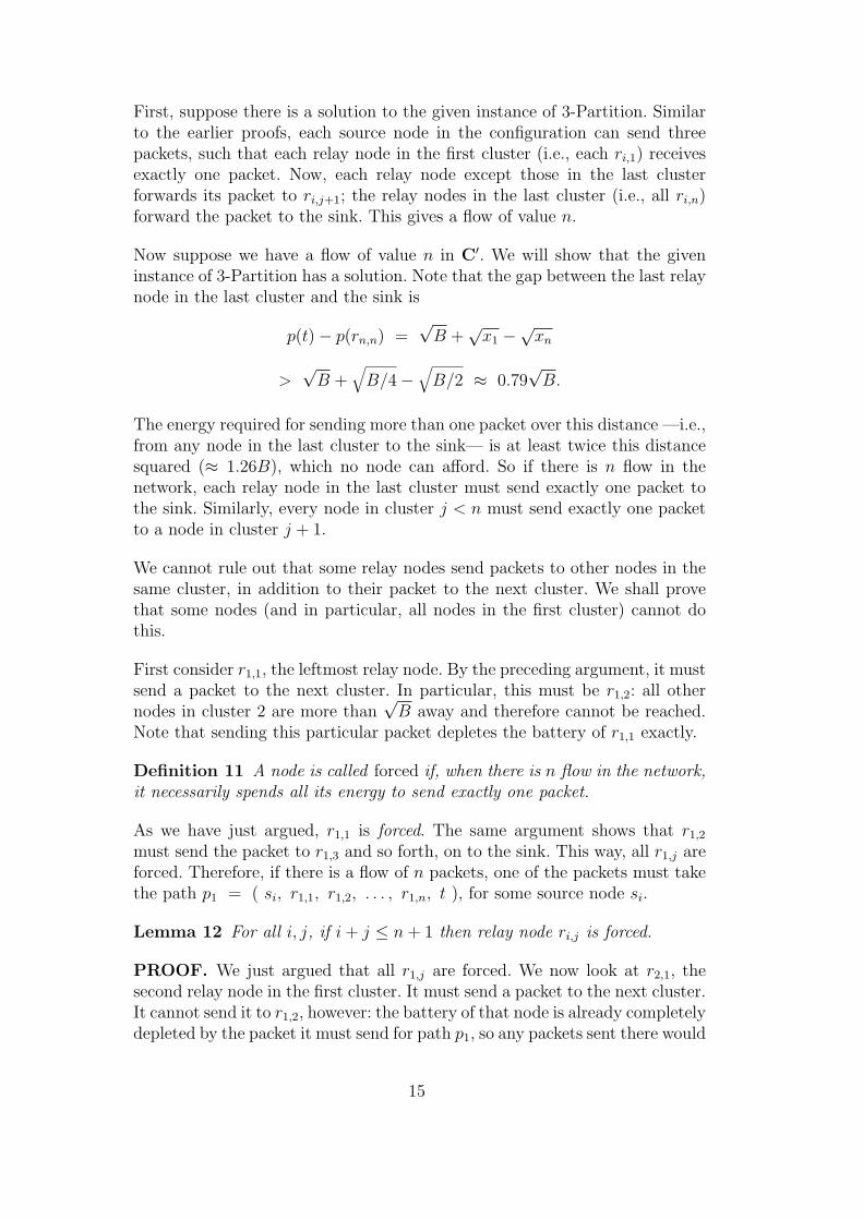
PROOF. Again, we give a pseudopolynomial reduction from 3-Partition.First we describe how to construct a geometric configuration C on the real line,where the Integer Max-Flow WSNC-problem is equivalent to a given instanceof 3-Partition. We then construct an equivalent configuration CP that can bedescribed in polynomial size. These steps together show that the Integer Max-Flow WSNC-problem is strongly NP-complete on geometric configurations.

Like before, we have m source nodes s1, . . . , sm. Each starts with B =∑

xi/menergy. These source nodes again play the role of the subsets and we place

10

s t

>√

B/4

<√

B/2

√B

ri

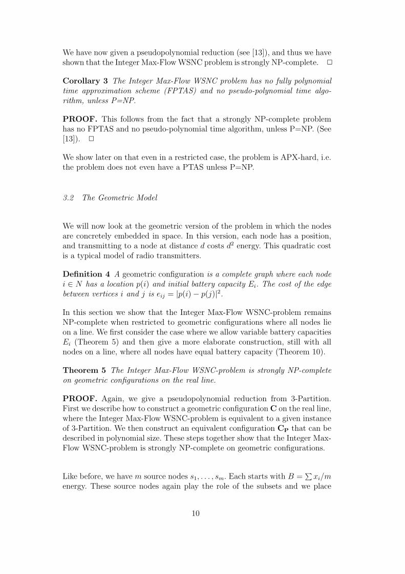
Fig. 1. Configuration C.

them all at the origin of our geometric configuration, i.e., p(si) = 0 for all i.(This also means that the cost of sending from one source node to another iszero, but such flow can be disregarded since all these nodes are sources.)

Corresponding to each xi ∈ S we have a ‘relay’ node ri that serves the samepurpose as before: to receive one packet from a source node, costing xi energyfor this source node, and relay the packet to the sink. By setting p(ri) =

√xi

we achieve that a source node must use xi energy to send a message to ri.

Finally, we place a sink node t with p(t) =√

B. We want each relay nodeto have just enough energy to send exactly one packet to the sink, so we setEri

= (p(t)− p(ri))2 = B + x− 2

√B√

x.

This concludes the construction of our geometric configuration C. The con-struction is illustrated in Figure 1.

Lemma 6 Suppose we have a flow of value n in C. Then every relay nodereceives exactly one packet from a source and sends it to the sink.

PROOF. If n packets reach the sink, then n packets must have left thesources. By the restriction on the values xi of the 3-Partition instance, eachedge leaving the sources costs strictly more than B/4 energy. Since the sourcenodes start with B energy, no source node can send more than 3 packets.There are only m = n/3 source nodes, so every source node must send exactly3 packets. In particular, no packets are sent directly from a source node to thesink, as this would use up all energy of the source node. Therefore, the sinknode only receives packets from relay nodes. No relay node can afford to sendmore than one packet to the sink, so in fact every relay node sends exactlyone packet to the sink. 2

Using Lemma 6, the following can now be shown in the same way as Theorem 2for the case on arbitrary graphs.

Proposition 7 The configuration C has a solution of the Integer Max-FlowWSNC-problem with n packets if and only if the corresponding 3-Partitioninstance is Yes.

11

Note that this does not yet give an NP-hardness proof for the Integer Max-Flow WSNC-problem on geometric configurations on the line, as configurationC has nodes at real-valued coordinates: the specification of the location of thepoints in C contains square roots. We shall now construct a geometric config-uration CP which is equivalent to C, but whose positions are all polynomiallyrepresentable rational numbers.

We do this by choosing the locations as integer multiples of some ε (value tobe determined later), rounding down. The initial power of the batteries alsoneeds to be quantized. We give the source nodes exactly B energy, which isalready integer. We give the relay nodes precisely enough energy to send onepacket to the sink; this amount can be calculated from the actual distance inCP.

Lemma 8 The value for ε can be chosen such that CP is equivalent to C andcan be represented in polynomial size.

PROOF. Consider a grid of precision ε, onto which the positions are roundeddown. Rounding down makes communication from sources to relay nodescheaper. For the NP-completeness construction we need that a source can-not send 4 packets. From the 3-Partition instance we have that the xi arestrictly bigger than B/4. Since the xi are integer, we have in particular thatthe xi ≥ B/4 + 1

4. This gives the following constraint on ε:

4(√

B + 1

4− ε

)2

> B.

This is equivalent to

ε <

√B + 1−

√B

2. (1)

That is, if we round coordinates down to a multiple of ε and (1) holds,no source node can send more than three packets. Note that this bound isΘ(1/

√B).

There is a further constraint on ε. We do not want to enable flows that donot correspond to a 3-Partition. Therefore, a source node should, with its Benergy, not be able to send packets to a set of relay nodes if the correspondingxi sum to strictly more than B. This gives the following constraint on ε, forall a, b, c ∈ S:

a + b + c ≥ B + 1 =⇒ (√

a− ε)2 + (√

b− ε)2 + (√

c− ε)2 > B.

This holds when the following condition holds; we solve the equation by settinga + b + c = B + 1.

ε <α−

√α2 − 3

3, where α =

√a +

√b +

√c.

12

This upperbound for ε is monotonically decreasing in α (for α >√

3) and istherefore minimized by maximizing α. This occurs at a = b = c = (B + 1)/3,giving

ε <

√B + 1−

√B√

3. (2)

This bound on ε is also Θ(1/√

B).

The number of gridpoints for a grid of length√

B is then

√B

ε=

√B

Θ(1/√

B)= Θ(B).

A position can therefore be represented in Θ(log B) space, just like the num-bers in the given 3-Partition instance (which are between B/4 and B/2).

Finally, we must specify ε. We can take e.g.

ε =1

5d√

Be.

This satisfies constraints (1) and (2) and can be written as a rational numberin polynomial space and time. Note that we can also compute the coordinatesof all relay nodes and the sink in polynomial time. 2

The proof of Theorem 5 now follows from Lemmata 6, 8 and Proposition 7:the Integer Max-Flow WSNC-problem is strongly NP-complete on geometricconfigurations, even when restricted to a line. 2

The nodes in CP have non-integer positions, but the following shows that thisis not essential.

Corollary 9 The Integer Max-Flow WSNC-problem is strongly NP-completeon geometric configurations on a line, where each node has an integer coordi-nate.

PROOF. Transform CP as follows. Multiply each position by ε−1 and eachbattery capacity by ε−2. This transformation assures that all coordinates areinteger, since all positions in CP are multiples of ε. Also, the transformedgeometric configuration is equivalent to CP, since for any set of distances di,a bound E and a value for ε, we have that the old situation is equivalent tothe transformed situation:

∑d 2

i ≤ E ⇐⇒∑(

di

ε

)2

≤ E

ε2. 2

13

s

t

>√

B/4√

B

ri,1 ri,2

ri,n

√B

√B

ri,n−1

Fig. 2. Configuration C′.

We finish this section by proving that Theorem 5 still holds when all batterycapacities are equal.

Theorem 10 The Integer Max-Flow WSNC-problem is strongly NP-completeon geometric configurations on the real line, even when all battery capacitiesare equal.

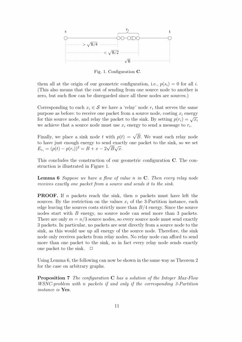
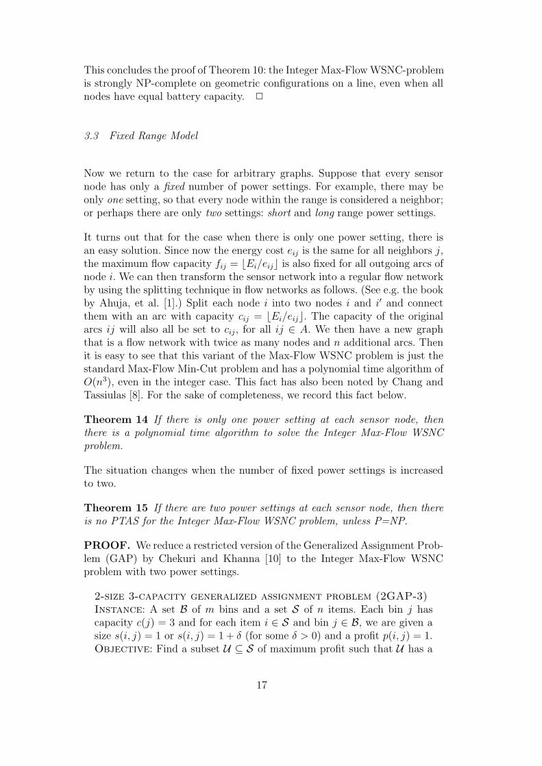
PROOF. Recall configuration C: source nodes, a cluster of relay nodes anda sink node. The battery capacity of the relay nodes was used to coerce eachrelay node to send exactly one packet, and to send it to the sink. Doing thisfor all relay nodes at once required varying battery capacities; we shall nowuse a more elaborate construction C′.

Where before we had a single cluster of relay nodes, we shall now have nclusters of relay nodes, spaced

√B apart. Then the geometric configuration

C′ is as follows.

• Source nodes: s1 . . . sm, with p(si) = 0.• Relay nodes: for each xi, there are n relay nodes, ri,1 . . . ri,n, with p(ri,j) =√

xi + (j − 1)√

B.

• A sink node t, with p(t) = n√

B +√

x1.• All nodes have starting battery capacity of B.

The configuration is visualized in Figure 2. We shall again prove that a flowof value n is possible in this configuration if and only if there is a 3-partitionin the given instance.

For convenience, let the xi be indexed in order of non-decreasing value. Fur-thermore, consider multiple relay nodes at the exact same location, whichoccurs if xi = xj for some i 6= j. Then the relay nodes for xi and xj are inter-changeable in any solution. This allows us to proceed in the following proofas if i < j implies xi < xj.

14

First, suppose there is a solution to the given instance of 3-Partition. Similarto the earlier proofs, each source node in the configuration can send threepackets, such that each relay node in the first cluster (i.e., each ri,1) receivesexactly one packet. Now, each relay node except those in the last clusterforwards its packet to ri,j+1; the relay nodes in the last cluster (i.e., all ri,n)forward the packet to the sink. This gives a flow of value n.

Now suppose we have a flow of value n in C′. We will show that the giveninstance of 3-Partition has a solution. Note that the gap between the last relaynode in the last cluster and the sink is

p(t)− p(rn,n) =√

B +√

x1 −√

xn

>√

B +√

B/4−√

B/2 ≈ 0.79√

B.

The energy required for sending more than one packet over this distance —i.e.,from any node in the last cluster to the sink— is at least twice this distancesquared (≈ 1.26B), which no node can afford. So if there is n flow in thenetwork, each relay node in the last cluster must send exactly one packet tothe sink. Similarly, every node in cluster j < n must send exactly one packetto a node in cluster j + 1.

We cannot rule out that some relay nodes send packets to other nodes in thesame cluster, in addition to their packet to the next cluster. We shall provethat some nodes (and in particular, all nodes in the first cluster) cannot dothis.

First consider r1,1, the leftmost relay node. By the preceding argument, it mustsend a packet to the next cluster. In particular, this must be r1,2: all othernodes in cluster 2 are more than

√B away and therefore cannot be reached.

Note that sending this particular packet depletes the battery of r1,1 exactly.

Definition 11 A node is called forced if, when there is n flow in the network,it necessarily spends all its energy to send exactly one packet.

As we have just argued, r1,1 is forced. The same argument shows that r1,2

must send the packet to r1,3 and so forth, on to the sink. This way, all r1,j areforced. Therefore, if there is a flow of n packets, one of the packets must takethe path p1 = ( si, r1,1, r1,2, . . . , r1,n, t ), for some source node si.

Lemma 12 For all i, j, if i + j ≤ n + 1 then relay node ri,j is forced.

PROOF. We just argued that all r1,j are forced. We now look at r2,1, thesecond relay node in the first cluster. It must send a packet to the next cluster.It cannot send it to r1,2, however: the battery of that node is already completelydepleted by the packet it must send for path p1, so any packets sent there would

15

not be able leave. The packet can be sent to r2,2, at cost exactly B, but itcannot be sent any further. So r2,1 is also forced, and again there is only onechoice for where to send the packet: via all the relay nodes for x2. This way,all r2,j are forced, except for r2,n: the distance between r2,n and t is less than√

B and its battery is not exhausted at once.

We now show the lemma with induction on i. We argued above the cases i = 1and i = 2. Suppose the result holds for i− 1, i ≥ 3. Consider a relay node ri,j,i+ j ≤ n+1. This node ri,j must send a packet to cluster j +1. Call the nodeit sends the packet to ri∗,j+1. Clearly, i∗ ≤ i, since otherwise the transmissionwould cost too much energy. We obtain a contradiction if i∗ < i. In that caseri∗,j is forced (induction hypothesis), so it sends a packet to ri∗,j+1. Also, ri∗,j+1

is forced (again, induction hypothesis), so it sends exactly one packet. Thusri,j cannot send a packet to ri∗,j+1. This leaves i∗ = i as the only option, andhence ri,j is forced. 2

In particular, we have that all ri,1 are forced. This means that all relay nodesin the first cluster receive exactly one packet from a source node, and spendall their energy sending this single packet to the next cluster. This is onlypossible if the original xi have a valid 3-partition: there is n flow in C′ if andonly if the original 3-Partition instance has a solution.

Again, we need to consider polynomial representation. We will round downthe positions in C′ to multiples of some ε and call the resulting geometricconfiguration C′

P.

Lemma 13 The value for ε can be chosen such that C′P is equivalent to C′

and can be represented in polynomial size.

PROOF. In addition to constraints (1) and (2) there is now an additionalconstraint. The construction requires that the forced nodes expend all theirenergy reaching a node at distance

√B. After rounding, this distance might

be only√

B − ε. This is no problem as long as the node’s remaining energyis not enough to reach any other node. The smallest distance between two

nodes, again considering the rounding, is√

B/2−√

(B − 1)/2− ε. This givesthe constraint

(√

B − ε)2 + (√

B/2−√

(B − 1)/2− ε)2 > B (3)

This bound on ε is Θ( 1B√

B) and can be satisfied by choosing e.g.

ε =1

5Bd√

Be.

This yields a total of Θ(nB2) grid points, leading to Θ(log nB) space pernode. 2

16

This concludes the proof of Theorem 10: the Integer Max-Flow WSNC-problemis strongly NP-complete on geometric configurations on a line, even when allnodes have equal battery capacity. 2

3.3 Fixed Range Model

Now we return to the case for arbitrary graphs. Suppose that every sensornode has only a fixed number of power settings. For example, there may beonly one setting, so that every node within the range is considered a neighbor;or perhaps there are only two settings: short and long range power settings.

It turns out that for the case when there is only one power setting, there isan easy solution. Since now the energy cost eij is the same for all neighbors j,the maximum flow capacity fij = bEi/eijc is also fixed for all outgoing arcs ofnode i. We can then transform the sensor network into a regular flow networkby using the splitting technique in flow networks as follows. (See e.g. the bookby Ahuja, et al. [1].) Split each node i into two nodes i and i′ and connectthem with an arc with capacity cij = bEi/eijc. The capacity of the originalarcs ij will also all be set to cij, for all ij ∈ A. We then have a new graphthat is a flow network with twice as many nodes and n additional arcs. Thenit is easy to see that this variant of the Max-Flow WSNC problem is just thestandard Max-Flow Min-Cut problem and has a polynomial time algorithm ofO(n3), even in the integer case. This fact has also been noted by Chang andTassiulas [8]. For the sake of completeness, we record this fact below.

Theorem 14 If there is only one power setting at each sensor node, thenthere is a polynomial time algorithm to solve the Integer Max-Flow WSNCproblem.

The situation changes when the number of fixed power settings is increasedto two.

Theorem 15 If there are two power settings at each sensor node, then thereis no PTAS for the Integer Max-Flow WSNC problem, unless P=NP.

PROOF. We reduce a restricted version of the Generalized Assignment Prob-lem (GAP) by Chekuri and Khanna [10] to the Integer Max-Flow WSNCproblem with two power settings.

2-size 3-capacity generalized assignment problem (2GAP-3)Instance: A set B of m bins and a set S of n items. Each bin j hascapacity c(j) = 3 and for each item i ∈ S and bin j ∈ B, we are given asize s(i, j) = 1 or s(i, j) = 1 + δ (for some δ > 0) and a profit p(i, j) = 1.Objective: Find a subset U ⊆ S of maximum profit such that U has a

17

feasible packing in B.

Chekuri and Khanna [10] show that the 2GAP-3 problem is APX-hard, henceit does not have a PTAS (unless P=NP).

Given an instance I of 2GAP-3 we create an instance I ′ of the Integer Max-Flow WSNC as follows. For each bin j ∈ B we have a source node j′ withenergy capacity Ej′ = 3. Corresponding to each item i ∈ S we have a relaynode i′. Each source node j′ is connected to each of the relay nodes i′ by an arcj′i′ with energy cost ej′i′ = 1 if s(i, j) = 1 and ej′i′ = 1+δ if s(i, j) = 1+δ. Wealso have one sink node t. Each of the sensor relay node i′ is further connectedto the sink node t and provided with just sufficient battery power to have thearc energy cost to send only one packet to the sink node, i.e., we set Ei′ = 1and ei′t = 1.

As each node i′ that represents an item can forward only one packet, eacharc of the form j′i′, j ∈ B, i ∈ S can also carry at most one packet. Thus,there is a one-to-one correspondence between integer flows in I fulfilling energyconstraints, and feasible packings of sets of items U ⊆ S: an item i that isplaced in bin j corresponds to a unit of flow that is transmitted from j′ toi′ and then from i′ to t. The value of the flow equals the total profit of thepacked items.

Thus, we can observe that our reduction is an AP-reduction. As AP-reductionspreserve APX-hardness (see e.g., [3]), we can conclude the theorem. 2

3.4 Approximation Algorithms

As the Integer Max-Flow WSNC problem has no PTAS (unless P=NP), ourhope is to find some approximation algorithms. We first give a very simpleapproximation algorithm. Then we give a slightly more involved algorithmwith a better approximation performance.

Theorem 16 There is a ρ-approximation algorithm for the Integer Max-FlowWSNC problem, where ρ = maxi∈N

maxij∈A eij

minij∈A eij.

PROOF. Convert the sensor network into a flow network as follows. We givethe edges unbounded capacity and we give each node i the capacity ci =b Ei

max eijc. Then a standard Max-Flow Min-Cut algorithm with node capacities

will yield a polynomial time algorithm that is at worst a ρ-factor from theoptimum. 2

Unfortunately the above approximation is not of constant ratio. Note that forthe fixed range model where each sensor has a constant number of fixed power

18

settings, the above algorithm does give a constant ratio approximation.

A better approximation algorithm is the following. The key idea is to firstsolve the fractional LP-formulation in polynomial time, and then try to finda large integer flow that is close to the optimum value.

Theorem 17 There is a polynomial time approximation algorithm for theInteger Max-Flow WSNC problem, which computes an integer maximum flowwith value Fapprox ≥ Foptimum− m, where m is the number of arcs of the graph.

PROOF. We give the proof for the case when there is only one source. It isa simple exercise to generalize the proof to the case with multiple sources.

First, we solve the relaxation of the problem optimally, i.e., we allow flows to beof real value. As this is an LP, the ellipsoid method gives us in polynomial timean optimal solution F ∗, that can be realized within the energy constraints.

We now find a large integer flow inside F ∗ in the following way. We use aninteger flow function F , which invariantly will map each arc ij to a non-negative integer fij with fij ≤ f ∗ij, and which has conservation of flows; i.e.,F will invariantly be a flow that fulfills the energy constraints. Initially, set Fto be 0 on all arcs.

Now, repeat the following step while possible. Find a path P from s to t, suchthat for each arc ij on the path, f ∗ij − fij ≥ 1. Let fP = minij∈P bf ∗ij − fijc bethe minimum over all arcs ij on the path P . Note that fP ≥ 1. Now add fP

to each fij for all arcs ij on the path P . Observe that the updated functionF fulfills the energy constraint conditions.

The process ends when each path from s to t contains an arc with f ∗ij−fij < 1.We note that F ∗−F is a flow, and standard flow techniques show that its valueis at most m, the number of arcs. (For let S be the set of nodes, reachablefrom s by a path with all arcs fulfilling f ∗ij − fij ≥ 1. Since t 6∈ S, (S, V −S) isa cut and its capacity with respect to the flow F ∗ − F is at most the numberof arcs across the cut.) Since the value of F ∗ is at least Foptimum, and hencethe value of F is at least Foptimum −m.

In each step of the procedure given above, we obtain at least one new arc ijwith f ∗ij − fij < 1; this arc will no longer be chosen in a path in a later step.Thus, we perform at most m steps. Each step can be done easily in lineartime. Hence, the algorithm is polynomial, using the time of solving one linearprogram plus O(m(n + m)) time for computing the approximate flow. 2

This algorithm is still not of constant ratio but we conjecture that it is a steptowards a 2-approximation algorithm.

19

4 Graphs with Bounded Treewidth

Many hard graph problems have polynomial (sometimes even linear) timealgorithms when restricted to graphs of bounded treewidth. This however isnot the case for the Integer Max-Flow WSNC problem: the problem remainshard. The treewidth parameter nicely delineates the classes of graphs for whichthe Integer Max-Flow WSNC is of apparently increasing complexity problemin the following manner.

• Graphs of treewidth one: These are just forests and have a very simplelinear time algorithm: remove all nodes that do not have a path to the sinkt; compute in the resulting tree in post-order for each node the number ofpackets it receives from its children and then the number of packets it cansend to its parent.

• Graphs of treewidth two: We show below that if there is a single source, andthe graph with an edge added between this single source and the sink nodehas treewidth two, then then there is a polynomial time algorithm for theInteger Max-Flow WSNC problem. The general case remains open.

• Graphs of bounded treewidth greater than two: We show that in this case,the problem is weakly NP-complete. We give a pseudo-polynomial time al-gorithm for this class.

• Graphs of unbounded treewidth: In this case, the problem is strongly NP-complete and even APX-hard, as shown in the previous section.

4.1 Graphs of Treewidth Two

In this section, we will show that the Integer Max-flow WSNC problem (withone source and one sink) is polynomial-time solvable if the treewidth of thegraph obtained by adding an edge from the source to the sink is bounded bytwo. While this is a somewhat specific case, we think this case is interestingbecause it partially bridges the gap between the trivial case of trees and theNP-hard case of treewidth three, and because the algorithmic technique is ofsome interest: unlike most algorithms that exploit treewidth, it does not usedynamic programming but a reduction strategy.

For a simple description of the algorithm, we generalize our problem in twoways. First, we allow parallel arcs. As a consequence, we need to change ournotation somewhat, and denote an arc with its name, instead of by the pairof endpoints. Parallel arcs may require a different energy per packet that istransmitted across them. Secondly, we assume that each arc p has a capacitycp. The capacity of an arc is a positive integer and denotes the maximumnumber of packets that can be transmitted across the arc.

20

If we have an instance without capacity, we can set for each arc p = ij,cp = bEi/eijc. Arcs with zero capacity can be removed.

Given a directed graph G = (N, A), with a source s and a sink t, we build theundirected graph Gu = (N, Au) as follows:

• There is an edge in Au between i and j, if and only if there is at least onearc from i to j and/or at least one arc from j to i in A.

• We add an edge from s to t.

Gu will be used as an auxiliary graph in subsequent constructions.

Theorem 18 The Integer Max-flow WSNC problem, with parallel arcs andarc capacities and with a single source s and sink t, can be solved in O(m log ∆)time on directed graphs G = (N, A), such that the graph (N, A ∪ st) hastreewidth at most two, where ∆ is the maximum outdegree of a node in G, andm = |A|.

Our algorithm is based upon the principle of reduction. While most algorithmsthat solve problems on graphs of small treewidth are based upon dynamicprogramming, some algorithms are also based upon reduction. (See e.g. [2,7].)

We first need a result on graphs with small treewidth.

Lemma 19 (Ramachandramurthi [19]) If Gu is a simple, undirected graphof treewidth at most k that is not a clique, then Gu has two non-adjacent ver-tices of degree at most k.

Corollary 20 If Gu is a simple, undirected graph of treewidth at most two,with at least three vertices, then there is a vertex of degree at most two that isneither the source s nor the sink t.

PROOF. If Gu is a clique, then it has exactly three vertices, and the resulttrivially holds. Otherwise, let i and j be the two non-adjacent vertices of degreeat most two, as indicated by Lemma 19. At least one of these two vertices isunequal to s and to t. 2

Now, we can repeat the following step. We first build Gu. Then, we find avertex i in Gu that is neither the source s nor the sink t, and that has degreeat most two in Gu (cf. Corollary 20). We now apply a reduction step, thattransforms G to an equivalent network without i, i.e., the number of verticesis decreased by one. We first describe the reduction step, and then will discussa more efficient implementation.

Let i be a vertex in Gu that is unequal to s and t, and that has degree at mosttwo.

21

If i has degree 0 then clearly we can remove i from G, and obtain an equivalentnetwork.

Suppose now that i has degree one in Gu. This means that there is a vertexj, such that all arcs in G with i as tail have j as head, and all arcs with i ashead have j as tail. Note that there always is an optimal flow that does nottransmit any packet from and to i. Thus, we can remove i and all arcs thathave i as one of its endpoints.

We now look at the most interesting case, namely that i has degree exactlytwo in Gu. Suppose the neighbors of i in Gu are j and k. The arcs with i asone of its endpoints are of the form:

• from j to i,• from i to k,• from k to i,• from i to j.

Call the arcs of the form ji and ik forward arcs, and arcs of the form ki andij backward arcs. Consider a flow with maximum value that has as additionalcondition that the total energy used by all nodes is minimal. In such a flow,either no packets will be transmitted over the forward arcs, or no packets willbe transmitted over the backward arcs. (If both packets are transmitted overforward and backward arcs, then we can cancel some and obtain a feasibleflow with the same value but smaller total energy.) For this reason, we canhandle forward and backward arcs independently.

First, consider all the forward arcs. We first compute a bound on the numberof packets that i can transmit to k, as follows. Suppose there are b number ofarcs ik. Sort these in order of non-decreasing energy per packet. Let the arcshave energy per packet e1 ≤ e2 ≤ · · · ≤ eb, and the corresponding capacitiesof the arcs c1, c2, . . . , cb. For all q, 1 ≤ q ≤ b, there is always an optimal flowthat only transmits a packet on the qth arc, when all pth arcs, with p < qhave totally used up their capacity. Thus, we can compute a bound Cik on thenumber of packets that i can transmit to k as follows.

If∑b

p=1 ep · cp ≤ Ei, then take Cik =∑b

p=1 cp. Otherwise, suppose that

q∑p=1

ep · cp ≤ Ei <q+1∑p=1

ep · cp

i.e., we have sufficient energy to use all the capacity of the first q arcs ik, butnot for the first q + 1 arcs. We thus use all capacity of these first q arcs, andpossibly some part of the capacity of the (q+1)th arc. Note that, after we usedup all the capacity of the first q arcs, we only have energy left to transmit at

22

most Ei −q∑

p=1

ep · cp

/eq+1

packets. Thus, we set

Cik =q∑

p=1

ep · cp +

⌊Ei −

∑qp=1 ep · cp

eq+1

⌋.

Observe that when Cik packets arrive at i, they all can be forwarded to k, butwe can never transmit more than Cik packets from i to k.

In the reduction, we build a new graph G′, where we have removed i and itsincident arcs, and added possibly a number of arcs between j and k (possiblyin both directions). G′ has vertex set N − i, and each arc in G that doesnot involve i is also an arc in G′. The arcs of the form jk in G′ are obtainedas follows.

Suppose there are d arcs of the form ji in G. Sort these in order of non-decreasing energy, and suppose these arcs have energies e1 ≤ e2 ≤ · · · ≤ ed,with corresponding capacities c1, c2, · · · , cd. Again, we may assume that wetransmit only packets over the arc with energy eq if we have used up allcapacities over all arcs with energy ep, p < q.

If∑d

p=1 cp ≤ Cik, then we replace each arc of the form ji in G by an arc ofthe form jk with the same energy cost and capacity: all packets transmittedthrough these arcs can be forwarded to k, so we have the same number ofpackets that can go from j to k, using the same amount of energy at j.Otherwise, suppose that for some node i with 0 ≤ i < s,

q∑p=1

cp ≤ Cik <q+1∑p=1

cp .

By the assumption made above, it follows that we will not be transmittingpackets over the arcs with energy larger than eq+1, and do not use the fullcapacity of the (q + 1)th arc. Thus, in G′ we take an arc jk with capacity cp

and energy cost ep for each p ≤ q, and an arc with capacity

c′q+1 = Cik −q∑

p=1

cp

and energy cost eq+1. (If c′q+1 = 0, we do not take the arc.) Note that the totalcapacity of the arcs jk is now Cik. It is not hard to see that we can transmitthe same number of packets in G from j to k via i as over the new arcs jk inG′.

For the backward arcs, we perform exactly the same step, except that the roles

23

of j and k are switched. In this fashion, we obtain an equivalent network, butnow with one less vertex.

This finishes the description of the reduction step. It is straightforward to seethat this step can be done in polynomial time. Different data structures mayhelp to speed up the performance of the reduction step.

Here, we use the mergeable heap data structure. This data structure performsthe following operations on a collection of elements. Each element has a key andpossibly more information stored. Our collection is partitioned into disjointsets. In our data structure, we can create a new set with one new element, witha key value and possibly other information; for a given set, obtain a pointerto the object that represents an element with maximum key value (and thusobtain this maximum, and possibly update the other information); for a givenset, we can delete this element with maximum key value; and for two givensets, we can take the disjoint union of the two sets, i.e., replace these sets bytheir disjoint union. Stylized implementations of mergeable heaps include theso called binomial heaps and the Fibonacci heaps, see e.g., [11, Chapters 19and 20].

Lemma 21 There is a data structure that allows unions of sets, obtainingthe element with maximum key, deleting the element with maximum key, andcreating new one element sets, such that each operation takes at most O(log d)time, where d is the maximum size of any set that is built.

Note that we cannot expect a much faster data structure, otherwise we cansort d elements using O(d) operations on the data structure; create a set foreach element, then take the union of all sets and then iteratively obtain anddelete the element with maximum key until no elements are left. The order inwhich the elements are deleted is sorted, from largest till smallest. Thus, O(d)operations on the data structure have to cost Ω(d log d) time, or Ω(log d) inthe worst case.

We now describe how the mergeable-heap data structure can be used to obtainan overall time of O(m log ∆), with ∆ the maximum outdegree of a node inG.

Note that the outdegree will never increase during a reduction step, and henceat each point in the algorithm, each node has an outdegree that is at most ∆.

We use a mergeable-heap data structure, with an element for each arc. Foreach node i and j, we have a set with all arcs from i to j, if there is at leastone such arc. We also maintain the graph Gu. As keys we use the cost of arcs;each arc has also its capacity stored. We further store the total capacity of allarcs from i to j; we denote this value by C ′

ij.

24

Now, a reduction step can be carried out as follows. We only consider theforward arcs as the backward arcs are similar. We use i, j, k, b, and d as inthe description of the reduction step for nodes of degree two in Gu, i.e., welook at the arcs ji and ik, and obtain arcs jk.

The procedure has three main steps.

First, we consider the arcs from i to k, and compute the value Cik, as describedabove. It is not hard to see that we can do this in O(d log d) time, if there ared such arcs. As each of the arcs from i to k can be deleted after this step, andi has outdegree at most ∆, the total time of this step over all reductions isbounded by O(m log ∆).

The second step is only carried out if C ′ij > Cik. For a faster implementation,

we do not sort the arcs from j to i, but instead we delete and/or update thecapacities of the arcs from j to i in order of non-increasing cost.

We repeat the following step, till C ′ji ≤ Cik. Obtain from the mergeable-heap

data structure an arc from j to i with maximum cost eji. Using the samenotation as above, suppose this is the pth arc, with cost ep and capacity cp. IfC ′

ij − cp ≥ Cik, then we delete this arc with maximum cost, and decrease C ′ij

by cp. This operation can be done in O(log ∆) time on the mergeable-heapdata structure. If C ′

ij − cp < Cik, then we must update the capacity of the arc:its new capacity must be Cik−Cji + cp, as Cji− cp is the sum of the capacitiesof the first p− 1 arcs from j to i (in order of non-decreasing cost). We also setCji to Cik.

One can verify that this step indeed gives the same collection of arcs andcapacities as the procedure described above where we first sorted the arcs inorder of non-decreasing cost. Note that all but possibly one of the forwardarcs that we considered are permanently deleted. Thus, if we delete d arcsin a reduction step, the step can be carried out in O((d + 1)∆) time, whichamounts to a total of O(m log ∆).

In the third step, all arcs from j to i now become arcs from j to k. We donot need to update this information for each arc, as it is sufficient if each setknows the endpoints of the arcs it represents. The third step has two cases. Ifbefore the reduction, there was a data structure with arcs from j to k, thenwe take the union of the data structure for arcs ji and arcs jk: these arcs nowall are arcs from j to k. If there were no arcs from j to k before the reduction,then the data structure for the arcs ji now acts as data structure for arcs jk.

The time for this third step thus is dominated by the time for one union inthe mergeable-heap data structure, i.e., it costs O(log ∆) per reduction. As weperform O(n) reduction, the total time over all third steps is O(n log ∆).

25

Thus, the total time is bounded by O(m log ∆). This completes the proof ofTheorem 18.

The problem for treewidth two graphs with multiple sources is still open.If we apply the construction from Section 4.2 that transforms a graph withtreewidth three with multiple sources to a graph with one source, then inmany cases, the treewidth grows to three. So the Integer Max-Flow WSNCproblem for general graphs of treewidth two remains open.

4.2 Graphs of Bounded Treewidth Greater than Two

Our second result on treewidth is that the Integer Max-Flow WSNC problemis NP-hard for graphs of treewidth three. This shows that a result like theprevious one for treewidth two graphs cannot be found when the treewidth isthree or more.

Theorem 22 The Integer Max-Flow WSNC problem is NP-hard for graphsof treewidth three.

The proof resembles the proof of strong NP-hardness for general graphs, butwe use here the (weak) NP-complete problem 2-partition instead of thestrong NP-complete problem 3-partition.

2-Partitioninstance: Given a multiset S of n positive integers a1, . . . , an and a positiveinteger B =

∑ni=1 ai/2.

question: Can S be partitioned into two subsets each of equal sum B.

PROOF. Given an instance I of 2-Partition, we create an instance I ′ ofthe Integer Max-Flow WSNC problem as follows.

Each number ai represents a sensor node wi each with energy Ei = B. Addi-tionally, we have a source node s and sink node t along with two special nodesv1 and v2, each of them with energy B. Now connect each vj (j = 1, 2) to eachwi with arc cost eji = ai. The source node s is connected to v1 and v2 witharc cost 1 each, and each node wi is connected to the sink node t with cost B.

Now, there is an energy constrained flow with n packets from s to t, if andonly if a1, . . . , an can be partitioned into two subsets, each of sum B.

If a1, . . . , an can be partitioned into two subsets S1, S2, each of sum B, thenwe can build a flow as follows: s transmits |S1| packets to v1 and |S2| packetsto v2. For each ai ∈ S1, v1 transmits a packet to wi, and similarly for eachai ∈ S2, v2 transmits a packet to wi, each packet consuming ai energy from

26

each node. Finally, each wi now transmits one packet to t. This fulfills therequirements of transmitting n packets from s to t.

Suppose now there is an energy constrained maximum flow of n packets froms to t. Note that each wi can transmit at most one packet to t, and as thereare n packets to t, each wi must transmit exactly one packet to t. So, for eachi, either v1 or v2 transmits a packet to wi. If v1 transmits a packet to wi, thenput ai in S1, otherwise put ai in S2. It is clear that S1 and S2 partition S. Foreach element ai ∈ S1, v1 must transmit a packet with cost ai, hence the sumof the elements in S1 is at most B. Similarly, the sum of the elements in S2 isat most B, and as the sum of all ai’s equals 2B, the sum of all elements in S1

equals B, and likewise for S2. 2

The constructed graph has a feedback vertex set of size two: if we remove v1

and v2 of the graph, we obtain a forest. Thus, it has treewidth at most three(see e.g. [5]). Its treewidth is also at least three, as it contains the completegraph K4 as a minor (remove w3, . . . , wn, contract s to v1, and w2 to t). Henceit has treewidth exactly three. The result also rules out a polynomial timealgorithm for the Integer Max-Flow WSNC problem on graphs of boundedtreewidth, unless P=NP.

However, we show now that there is a pseudo-polynomial time algorithm when-ever the treewidth is bounded.

Theorem 23 The Integer Max-Flow WSNC problem can be solved in pseudo-polynomial time on graphs of bounded treewidth.

PROOF. We begin with a number of auxiliary definitions. A boundary di-rected graph is a triple (N, A, X), with (N, A) a directed graph, and X ⊆ N aset of distinguished vertices, called the boundary.

Suppose (N ′, A′, X) is a boundary directed graph with (N ′, A′) a subgraph ofthe given graph G = (N, A), with given costs and energies, and source s andsink t.

A partial energy constrained flow, or in short pecf, in this boundary directedgraph is a function that assigns to each arc ij in A′ a flow-value, such that

• for all i ∈ N ′ − s, t, the inflow of i equals the outflow of i, and• for all i ∈ N ′, the cost of the outflow of i is at most Ei.

The signature of a pecf is a pair (q, ε), with q a function that maps each i ∈ Xto the outflow of i minus the inflow of i:

q(i) =∑ij∈A

fij −∑ji∈A

fji

27

and ε a function that maps each i ∈ X to the used energy at sensor i:

ε(i) =∑ij∈A

fij · eij .

For ease of notation, we also use fij when there is no arc ij ∈ A; in such a case,fij = 0. The algorithm we will design uses a special type of tree decomposition:a nice tree decomposition where, in addition to the usual requirements, weassume that the root of the tree decomposition r has a bag that contains onlys: Xr = s. A nice tree decomposition has four types of nodes:

• Leaf nodes: node α which is a leaf of the tree with |Xα| = 1.• Introduce nodes: node α with one child β with Xα = Xβ ∪ i for some

node i.• Forget nodes: node α with one child β, with Xα = Xβ −i for some node

i.• Join nodes: node α with two children β, γ with Xα = Xβ = Xγ.

For each node α in the tree decomposition, we define a boundary directedgraph Gα = (Nα, Aα, Xα), with Nα the set of all vertices in Xα or Xβ with βa descendant of α, and Aα the set of all arcs in A between vertices in Nα.

A small modification of the construction in [6] shows that we can obtain inlinear time, given a tree decomposition of width at most k of a graph G, anice tree decomposition of G of width at most k, such that the root node rhas Xr = s.

Our algorithm mainly consists of iteratively computing for each node α in thetree decomposition a table consisting of all signatures of all pecf’s in Gα. Thetables are computed in post-order, i.e., we compute a table for a node whenthe tables of its children are known.

Note that the size of each table is pseudo-polynomial, as there are pseudo-polynomially many signatures of pecf’s in Gα: for each i ∈ Xα, ε(i) is aninteger between 0 and Ei, the outflow of i is an integer between 0 and Ei, theinflow of i is an integer between 0 and

∑ji∈A Ej, and hence q(i) is an integer

between −∑ji∈A Ej and Ei.

We now give for each of the four types of nodes a description of a procedurethat computes for a node α the table of all signatures of all pecf’s in Gα, givensuch tables for the children of α.

Leaf nodes: It is trivial to see that the table can be computed directly for aLeaf node.

28

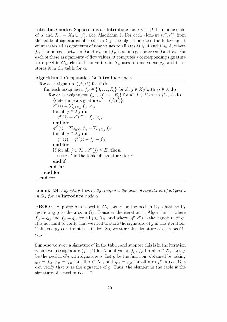
Introduce nodes: Suppose α is an Introduce node with β the unique childof α and Xα = Xβ ∪ i. See Algorithm 1. For each element (qσ, εσ) fromthe table of signatures of pecf’s in Gβ, the algorithm does the following. Itenumerates all assignments of flow values to all arcs ij ∈ A and ji ∈ A, wherefij is an integer between 0 and Ei, and fji is an integer between 0 and Ej. Foreach of these assignments of flow values, it computes a corresponding signaturefor a pecf in Gα, checks if no vertex in Xα uses too much energy, and if so,stores it in the table for α.

Algorithm 1 Computation for Introduce nodes

for each signature (qσ, εσ) for β dofor each assignment fij ∈ 0, . . . , Ei for all j ∈ Xβ with ij ∈ A do

for each assignment fji ∈ 0, . . . , Ej for all j ∈ Xβ with ji ∈ A dodetermine a signature σ′ = (q′, ε′)εσ′(i) =

∑j∈Xβ

fij · eij

for all j ∈ Xβ doεσ′(j) = εσ(j) + fji · eji

end forqσ′(i) =

∑j∈Xβ

fij −∑

j∈Xβfji

for all j ∈ Xβ doqσ′(j) = qσ(j) + fji − fij

end forif for all j ∈ Xα: εσ′(j) ≤ Ej then

store σ′ in the table of signatures for αend if

end forend for

end for

Lemma 24 Algorithm 1 correctly computes the table of signatures of all pecf ’sin Gα for an Introduce node α.

PROOF. Suppose g is a pecf in Gα. Let g′ be the pecf in Gβ, obtained byrestricting g to the arcs in Gβ. Consider the iteration in Algorithm 1, wherefij = gij and fji = gji for all j ∈ Xβ, and where (qσ, εσ) is the signature of g′.It is not hard to verify that we need to store the signature of g in this iteration,if the energy constraint is satisfied. So, we store the signature of each pecf inGα.

Suppose we store a signature σ′ in the table, and suppose this is in the iterationwhere we use signature (qσ, εσ) for β, and values fij, fji for all j ∈ Xβ. Let g′

be the pecf in Gβ with signature σ. Let g be the function, obtained by takinggij = fij, gji = fji for all j ∈ Xβ, and gj` = g′j` for all arcs j` in Gβ. Onecan verify that σ′ is the signature of g. Thus, the element in the table is thesignature of a pecf in Gα. 2

29

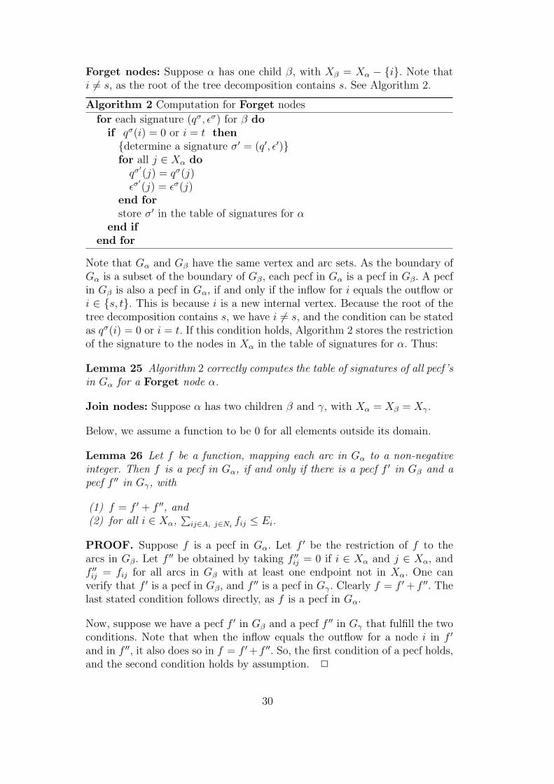
Forget nodes: Suppose α has one child β, with Xβ = Xα − i. Note thati 6= s, as the root of the tree decomposition contains s. See Algorithm 2.

Algorithm 2 Computation for Forget nodes

for each signature (qσ, εσ) for β doif qσ(i) = 0 or i = t thendetermine a signature σ′ = (q′, ε′)for all j ∈ Xα do

qσ′(j) = qσ(j)εσ′(j) = εσ(j)

end forstore σ′ in the table of signatures for α

end ifend for

Note that Gα and Gβ have the same vertex and arc sets. As the boundary ofGα is a subset of the boundary of Gβ, each pecf in Gα is a pecf in Gβ. A pecfin Gβ is also a pecf in Gα, if and only if the inflow for i equals the outflow ori ∈ s, t. This is because i is a new internal vertex. Because the root of thetree decomposition contains s, we have i 6= s, and the condition can be statedas qσ(i) = 0 or i = t. If this condition holds, Algorithm 2 stores the restrictionof the signature to the nodes in Xα in the table of signatures for α. Thus:

Lemma 25 Algorithm 2 correctly computes the table of signatures of all pecf ’sin Gα for a Forget node α.

Join nodes: Suppose α has two children β and γ, with Xα = Xβ = Xγ.

Below, we assume a function to be 0 for all elements outside its domain.

Lemma 26 Let f be a function, mapping each arc in Gα to a non-negativeinteger. Then f is a pecf in Gα, if and only if there is a pecf f ′ in Gβ and apecf f ′′ in Gγ, with

(1) f = f ′ + f ′′, and(2) for all i ∈ Xα,

∑ij∈A, j∈Ni

fij ≤ Ei.

PROOF. Suppose f is a pecf in Gα. Let f ′ be the restriction of f to thearcs in Gβ. Let f ′′ be obtained by taking f ′′ij = 0 if i ∈ Xα and j ∈ Xα, andf ′′ij = fij for all arcs in Gβ with at least one endpoint not in Xα. One canverify that f ′ is a pecf in Gβ, and f ′′ is a pecf in Gγ. Clearly f = f ′ + f ′′. Thelast stated condition follows directly, as f is a pecf in Gα.

Now, suppose we have a pecf f ′ in Gβ and a pecf f ′′ in Gγ that fulfill the twoconditions. Note that when the inflow equals the outflow for a node i in f ′

and in f ′′, it also does so in f = f ′+f ′′. So, the first condition of a pecf holds,and the second condition holds by assumption. 2

30

We now compute the table of the signatures of the pecf’s in Gα. See Algorithm3.

Algorithm 3 Computation for Join nodes

for each signature (qσ, εσ) for β dofor each signature (qσ′ , εσ′) for γ dodetermine a signature σ′ = (q′, ε′)for all i ∈ Xα do

εσ′′(i) = εσ(i) + εσ′(i)qσ′′(i) = qσ(i) + qσ′(i)

end forif for all i ∈ Xα: εσ′′(i) ≤ Ei then

store σ′′ in the table of signatures for αend if

end forend for

We now establish its correctness.

Lemma 27 Algorithm 3 correctly computes the table of the signatures ofpecf ’s in Gα for a Join node α.

PROOF. One can verify that if σ is the signature of a pecf f ′ in Gβ, andσ′ is the signature of a pecf f ′′ in Gγ, then the signature σ′′ as computed byAlgorithm 3 is the signature of f ′ + f ′′. Correctness follows now directly fromLemma 26. 2

We now complete the proof of Theorem 23. Using the procedures for thedifferent types of nodes, we can compute all tables, in post-order. As eachtable has pseudo-polynomial size, and the time per table is polynomial in thenumber of signatures of the tables of the children for Join, Introduce andForget nodes, and O(1) for Leaf nodes, this costs pseudo-polynomial time.

Lemma 28 F packets can be transmitted from s to t in the network, if andonly if the table of the root r of the tree decomposition contains a signature(q, ε) for some ε with q(s) = F .

PROOF. Note that Gr has the same vertices and arcs as G. Thus, a pecf inG is a flow in G that fulfills the energy constraint, and vice versa. The valueof a flow with signature (q, ε) equals q(s). Now the lemma follows. 2

After all tables have been computed, we can find the value of the optimal flowby inspecting the table of the root node: by Lemma 28, this value equals themaximum F , such that a signature (q, ε) for some ε with q(s) = F belongs tothe table of the root of the tree decomposition. With additional bookkeeping,one can also find the corresponding flow. 2

31

5 Conclusion

The Maximum Flow WSNC problem is an interesting and relevant problem,with practical implications in the context of wireless ad hoc networks. In thispaper, we studied the integer variant of the problem. We obtained a goodpolynomial time approximation algorithm for the problem, which is howevernot of constant performance ratio. We also studied how the complexity of theproblem depends on the treewidth of the network. We found that except forthe case where each sensor has one fixed power setting or when the underlyinggraph is of treewidth two with an edge joining the source and sink nodes, theproblem is weakly NP-complete for bounded treewidth greater than two. It isstrongly NP-complete for networks of unbounded treewidth and in fact evenAPX-hard. It is also strongly NP-complete on geometric configurations on aline.

Acknowledgements

We thank Alex Grigoriev, Han Hoogeveen, Arie Koster, Erik van Ommerenand Gerhard Woeginger for fruitful discussions and helpful comments.

References

[1] R. K. Ahuja, T. L. Magnanti, and J. B. Orlin. Network Flows: Theory,Algorithms, and Applications. Prentice Hall, Upper Saddle River, NJ, USA,1993.

[2] S. Arnborg, B. Courcelle, A. Proskurowski, and D. Seese. An algebraic theoryof graph reduction. J. ACM, 40:1134–1164, 1993.

[3] G. Ausiello, P. Crescenzi, G. Gambosi, V. Kann, A. Marchetti-Spaccamela,and M. Protasi. Complexity and Approximation: Combinatorial OptimizationProblems and Their Approximability Properties. Springer, Berlin, 1999.

[4] H. L. Bodlaender. A tourist guide through treewidth. Acta Cybernetica, 11:1–23, 1993.

[5] H. L. Bodlaender. A partial k-arboretum of graphs with bounded treewidth.Theor. Comp. Sc., 209:1–45, 1998.

[6] H. L. Bodlaender and T. Kloks. Efficient and constructive algorithms for thepathwidth and treewidth of graphs. J. Algorithms, 21:358–402, 1996.

[7] H. L. Bodlaender and B. van Antwerpen-de Fluiter. Reduction algorithms forgraphs of small treewidth. Information and Computation, 167:86–119, 2001.

32

[8] J. Chang and L. Tassiulas. Fast approximate algorithms for maximum lifetimerouting in wireless ad-hoc networks. In Proceedings Networking 2000, pages702–713, 2000.

[9] J. Chang and L. Tassiulas. Maximum lifetime routing in wireless sensornetworks. IEEE/ACM Transaction on Networking, 12(4):609–619, 2004.

[10] C. Chekuri and S. Khanna. A polynomial time approximation scheme for themultiple knapsack problem. SIAM J. Comput., 35(3):713–728, 2005.

[11] T. H. Cormen, C. E. Leiserson, R. L. Rivest, and C. Stein. Introduction toAlgorithms, Second Edition. MIT Press, Cambridge, Mass., USA, 2001.

[12] P. Floreen, P. Kaski, J. Kohonen, and P. Orponen. Exact and approximatebalanced data gathering in energy-constrained sensor networks. Theor. Comp.Sc., 344(1):30–46, 2005.

[13] M. R. Garey and D. S. Johnson. Computers and Intractability, A Guide to theTheory of NP-Completeness. W.H. Freeman and Company, New York, 1979.

[14] N. Garg and J. Konemann. Faster and simpler algorithms for multi-commodityflow and other fractional packing problems. In Proceedings of the 39th AnnualSymposium on Foundations of Computer Science, pages 300–309, 1998.

[15] W. R. Heinzelman, A. Chandrakasan, and H. Balakrishnan. Energy-efficientcommunication protocol for wireless microsensor networks. In Proceedings 33rdHawaii International Conference on System Sciences HICSS-33, 2000.

[16] B. Hong and V. K. Prasanna. Maximum lifetime data sensing and extractionin energy constrained networked sensor systems. J. Parallel and DistributedComputing, 66(4):566–577, 2006.

[17] K. Kalpakis, K. Dasgupta, and P. Namjoshi. Efficient algorithms for maximumlifetime data gathering and aggregation in wireless sensor networks. ComputerNetworks, 42(6):697–716, 2003.

[18] F. Ordonez and B. Krishnamachari. Optimal information extraction inenergy-limited wireless sensor networks. IEEE Journal on Selected Areas inCommunications, 22(6):1121–1129, 2004.

[19] S. Ramachandramurthi. The structure and number of obstructions to treewidth.SIAM J. Disc. Math., 10:146–157, 1997.

[20] Y. Xue, Y. Cui, and K. Nahrstedt. Maximizing lifetime for data aggregation inwireless sensor networks. Mobile Networks and Applications, 10:853–864, 2005.

[21] F. Zhao and L. Guibas. Wireless Sensor Networks: An Information ProcessingApproach. Morgan Kaufman, 2004.

33