ARTICLE IN PRESS

Contents lists available at ScienceDirect

Int. J. Production Economics

Int. J. Production Economics 120 (2009) 315–326

0925-52

doi:10.1

� Cor

E-m

journal homepage: www.elsevier.com/locate/ijpe

Backup strategy for robots’ failures in an automotiveassembly system

Tomer Kahan a, Yossi Bukchin a,�, Roland Menassa b, Irad Ben-Gal a

a Department of Industrial Engineering, Faculty of Engineering, Tel-Aviv University, Tel-Aviv 69978, Israelb Manufacturing Systems Research, GM Research & Development, MC-480-106-359, 30500 Mound Road, Warren, MI 48090-9055, USA

a r t i c l e i n f o

Article history:

Received 23 October 2006

Accepted 16 September 2007Available online 18 January 2009

Keywords:

Automotive industry

Assembly lines

Spot welding

Robot failures

Line balancing

73/$ - see front matter & 2009 Elsevier B.V. A

016/j.ijpe.2007.09.015

responding author. Tel.: +972 3 6407941; fax:

ail address: bukchin@eng.tau.ac.il (Y. Bukchin

a b s t r a c t

Automotive assembly lines are often characterized by robots’ failures that may result in

stoppages of the lines and manual backup of tasks. The phenomena tend to impair

throughput rate and products’ quality. This paper presents a backup strategy in which

working robots perform tasks of failed robots. The proposed Mixed-Integer Linear-

Programming based approach minimizes the throughput loss by utilizing the robots’

redundancy in the system. Two algorithms are developed to comply with stochastic

conditions of a real-world environment. The performance of these algorithms is

compared with several heuristics, and the downstream-backup based algorithm is

found superior to all other methods.

& 2009 Elsevier B.V. All rights reserved.

1. Introduction: body-shop systems in the automotiveindustry

High-volume body-shop systems in the automotiveindustry often consist of a series of assembly zones thatare serially connected via automated material handling(MH) systems. A zone contains several robotic cells (alsocalled stations), each of which consist of several weldingrobots that are working simultaneously. The automatedMH system is used for feeding the stations with parts thatare assembled (welded) to the vehicle body. These MHsystems are usually asynchronous where carriers cancirculate if they are not blocked or starved.

Weld spots are grouped on the basis of their location inthe vehicle body and performed sequentially by a singlewelding robot. There are two types of weld spots:dimensional control welds (DCWs) and respot welds(RSPs). In DCWs, a new part is welded to the vehicle’sbody to define a new geometry of the vehicle. A stationwhich performs DCWs is usually facilitated by an auto-

ll rights reserved.

+972 3 6407669.

).

mated MH system (and sometimes by another dedicatedrobot) which transfers the parts that have to beassembled. RSPs are performed on an existing geome-try—no new part is assembled, and the sole purpose ofthe RSPs is to strengthen the vehicle’s body.

Each robot can weld a single group of spots or multiplegroups of spots in a single work cycle. The welding task,performed by a spot welding-gun, consists of the robotmotion from the ‘‘Home position’’ to the welding area andback to the ‘‘Home’’ position, in addition to the timededicated to each welding spot.

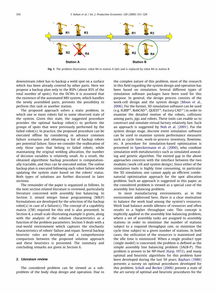
The problem addressed in this paper refers to asituation, depicted in Fig. 1, in which one robot or multiplerobots fail during the operation time. The proposedrecovery plan or a backup plan should then indicatewhich robot(s) replace the failed ones during the repairperiod. The backup plan aims at minimizing the failureseffects on the throughput rate.

It is assumed that the capability of each robot, in termsof the weld spots it can perform, is known and given, aswell as the precedence relationships among various groupsof spots. The precedence relationships indicate theassembly sequence among groups of spots, and eliminateinfeasible situations. For example, a situation where a

ARTICLE IN PRESS

Station A Station B

R1 R3

R4R2

R1 R3

R4R2

Fig. 1. The problem illustration: robot R4 in station A fails and is replaced by robot R4 in station B.

T. Kahan et al. / Int. J. Production Economics 120 (2009) 315–326316

downstream robot has to backup a weld spot on a surfacewhich has been already covered by other parts. Here wepropose a backup plan only to the RSPs (about 85% of thetotal number of spots). For the DCWs it is assumed thatthe existence of the automated MH system, which handlesthe newly assembled parts, prevents the possibility toperform this task in another station.

The proposed approach solves a static problem, inwhich one or more robots fail in some observed state ofthe system. Given this state, the suggested procedureprovides the optimal backup robot(s) to perform thegroups of spots that were previously performed by thefailed robot(s). In practice, the proposed procedure can beexecuted offline by considering in advance commonfailure scenarios and obtaining a list of backup robotsper potential failure. Since we consider the reallocation ofonly those spots that belong to failed robots, whilemaintaining the original welding allocation, the numberof decision variables is relatively small. As a result, theobtained algorithmic backup procedure is computation-ally tractable, and thus can be executed online. The onlinebackup plan is executed following each robot failure whileupdating the system state based on the robots’ status.Both types of solutions are further discussed in latersections.

The remainder of the paper is organized as follows. Inthe next section related literature is reviewed, particularlyliterature concerned with assembly line balancing. InSection 3, mixed integer linear programming (MILP)formulations are developed for the selection of the backuprobot(s) in case of a failure(s). The concept of a capabilitymatrix (CM) required for this end is also presented. InSection 4, a small scale illustrating example is given, alongwith the analysis of the solution characteristics as afunction of the problem parameters. Section 5 deals with areal-world environment which captures the stochasticcharacteristics of robots’ failure and repair. Several backupheuristic rules are developed and a comprehensivecomparison between the proposed solution approachand these heuristics is presented. The summary andconcluding remarks are given in Section 6.

2. Literature review

The considered problem can be viewed as a sub-problem of the body shop design and operation. Due to

the complex nature of this problem, most of the researchin this field regarding the system design and operation hasbeen based on simulation. Several different types ofsimulation software packages have been used for thispurpose. In general, the design process consists of thework-cell design and the system design (Moon et al.,2006). For the former, 3D simulation software can be used(e.g. IGRIPs, RobCADs, QUESTs, Factory CADs) in order toexamine the detailed motion of the robots, collisionsamong parts, jigs and robots. These tools can enable us toconstruct and simulate virtual factory relatively fast. Suchan approach is suggested by Noh et al. (2001). For thesystem design stage, discrete event simulation softwarecan be used to examine system performance measuressuch as cycle time, work-in-process inventory, flowtime,etc. A procedure for simulation-based optimization ispresented in Spieckermann et al. (2000), who combinesimulation with metaheuristics such as simulated anneal-ing and genetic algorithm. The existed gap in the aboveapproaches concerns with the interface between the twomodules (work cell and system design). Since either of thesimulation tools is highly time consuming, in particularthe 3D simulation, one cannot apply an efficient combi-natorial optimization approach for the spot allocationproblem. Such an approach is suggested in this paper, asthe considered problem is viewed as a special case of theassembly line balancing problem.

In most manufacturing environments, as in theenvironment addressed here, there is a clear motivationto balance the work load among the system’s resources.Work load balance avoids idleness of resources and oftenresults in a higher throughput rate. This concept isexplicitly applied in the assembly line balancing problem,where a set of assembly tasks are assigned to assemblystations in order to minimize the number of stationssubject to a required throughput rate, or minimize thecycle time subject to a given number of stations. In bothcases, the utilization of the resources is maximized andthe idle time is minimized. When a single product type(single model) is concerned, the problem is defined as thesimple assembly line balancing problem (SALB-P). Thisproblem is proven to be NP-Hard (Karp, 1972), and manyoptimal and heuristic algorithms for this problem havebeen developed during the last 50 years. Baybars (1986)presents a survey on optimal procedures developed forthis problem. Scholl and Becker (2006) present a state ofthe art survey of optimal and heuristic procedures for the

ARTICLE IN PRESS

T. Kahan et al. / Int. J. Production Economics 120 (2009) 315–326 317

SALB-P. Amen (2000) presents a survey on heuristicapproaches for assembly line balancing when cost isexplicitly considered. The assembly line balancing litera-ture consists of many variations of the basic problem, suchas assembly lines with stochastic task times, mixed-modellines (where different product types are assembled on thesame line), paced lines versus un-paced lines, equipmentselection, etc. Ghosh and Gagnon (1989) review optimaland heuristic procedures for several variations of theproblem. An up-to-date survey is provided in Becker andScholl (2006), which addresses the generalized assemblyline balancing (GALB-P). Boysen et al. (2008) addressesthe gap between research and practice. They classify thevariations of the line balancing problem and suggestrelevant models for the real-world problems.

Although most traditional literature addresses manualassembly lines, some papers take into account theequipment required for the assembly process. Gravesand Holmes Redfield (1988) consider the mixed-modelassembly line design problem, where each task can beperformed by one or more alternative types of equipment.Assuming a fixed sequence of the assembly tasks andlarge similarities among different products, they suggest aprocedure for the design process, consisting of thesimultaneous task assignment and equipment selection.Rubinovitz and Bukchin (1993), and later on Bukchin andTzur (2000), address a similar problem, where a singlemodel is concerned with a relatively flexible assemblysequence, expressed by a precedence diagram. The taskassignment, along with equipment selection out of multi-ple alternatives, is performed by using a branch andbound optimal procedure for moderate sized problems.Another branch and bound based heuristic is proposed forsolving large scale problems. Bukchin and Rubinovitz(2003) extend the above problem to address the possibi-lity to apply parallel stations in the assembly line.

The problem considered in this paper can be viewed asanother variation of the classic assembly line balancingproblem, where the assembly equipment, spot-weldingrobots in this case, is taken into account. Nevertheless,unlike the above, an operational problem rather than adesign problem is considered here, where the robots arealready placed in stations. Each time one or more robotsfail, the problem of assigning the group(s) of spots (tasks)of the failed robot(s) to other working robot(s) can beconsidered as a re-balancing problem. Fortunately, sinceonly the failed groups (i.e., the groups that were assignedto the failed robot) are to be reassigned to the backuprobots, it is found that relatively large problems can besolved in a relatively reasonable amount of time.

3. Spot re-allocation models

3.1. Preliminaries and definitions

The problem of spots reallocation due to a robot’sfailure can be addressed in three hierarchical levels:(level 1) single-robot backup; (level 2) group allocationbased multi-robot backup; and (level 3) spot allocationbased multi-robot backup. In the first level, the whole

work content, consisting of one or several groups ofwelding spots of the failed robot(s), is reallocated to asingle backup robot. In the second level, each groupperformed by the failed robot is reallocated as a whole;yet, different groups of spots can be allocated to differentbackup robots. In the third level, any of the spots in eachof the failed groups can be individually allocated amongdifferent backup robots.

There is a clear tradeoff between the quality of theproposed solution and the required algorithmic complex-ity. The proposed solution framework is general enough tobe implemented in each of these hierarchical levels.Nevertheless, the proposed solution approach focuses onthe first two hierarchical levels from practical considera-tions. Splitting spots within a group (the third hierarchicallevel) might be attractive with regard to the cycle timereduction. However, the current available technology,both at the controllers and the robotics stations, do notenable an efficient execution at this level.

As discussed above, the determination of the backuprobot(s) is somewhat similar to the re-balancing of anassembly line which aims at minimizing the cycle time.Consequently, the proposed MILP, on which the solutionapproach is based, is an enhanced version of similarformulations known in the area of assembly line balan-cing. In the proposed formulation, robots and groups ofspots are analogous to the stations and tasks in thetraditional assembly line, respectively. Consequently, weassume that the robot load is equal to the summation ofall welding times of the groups of spots assignedto this robot, and the line cycle time is determinedby the most loaded robot. In the proposed model weconsider only the group of spots of the failed robot(s)to be reallocated, while shifting groups of working robotsis not allowed. Accordingly, we expect the number ofinteger variables to be much smaller with respectto the assembly line balancing problems. As noted above,the reduction in the number of variables leads to asolution which can be attained in a relatively smallamount of time. Next we present the used notation andformulations.

Notation

Sets and parameters

I set of total groups of spotsIW set of total groups of spots assigned to working

robots, IWDI

IF set of total groups of spots assigned to failedrobots, IF

¼ I=IW

R set of all the robots located in the assembly lineRW set of working robots, RWDR

RF set of failed robots, RF¼ R\RW

Ti performance time of group of spots i (includingsetup)

IPWi set of immediate predecessors of group of spots i

assigned to working robotsISW

i set of immediate successors of group of spots i

assigned to working robots

ARTICLE IN PRESS

T. Kahan et al. / Int. J. Production Economics 120 (2009) 315–326318

IPFi set of immediate predecessors of group of spots i

assigned to failed robotsISF

i set of immediate successors of group of sport i

assigned to failed robots

MatricesTwo matrices describe the current and the potential

work allocation in the system. The former is given by theinitial matrix (IM) and the latter given by the CM. Theentries in these matrices satisfy the following rule.

IMir ¼

1; if a group of spots i is performed by robot

r the system’s initial state

0 otherwise

8>><>>:8i 2 I; 8r 2 R,

CMir ¼1; if a group spots i can performed by robot r

0 otherwise;

(

8i 2 I; 8r 2 R

Note that CMirXIMir 8i 2 I; 8r 2 R.A third matrix, which represents the solution of the

backup problem, is the recovery matrix (RM) and will beexplained later.

Decision variables

xr ¼1; if robot r is a backup robot

0 otherwise

�8r 2 R,

c—cycle time of the system

xr ¼1; if group spots i is performed by robot r after failure

0 otherwise;

(

8i 2 IF ; 8r 2 RW

Prior to implementing the solution procedure, the CM

and the precedence diagram should be obtained. The CMcaptures the redundancy of the system and the capabilityof different robots with regard to performing differentgroups of spots. The precedence diagram consists of theprecedence constraints among groups. The CM, along withthe precedence diagram, establish the sets of constraintsfor the backup strategy.

As noted above, each element CMir of the CM is equal to1 if group of spots i can be performed by robot r and 0otherwise. The CM is generated on the basis of the initialmatrix, IM. Each row of IM is examined with respect tothose robots that are capable of performing the respectivegroup of spots, in addition to the originally allocatedrobot. For each robot r, which is capable to backup groupof spots i, we set Cmir ¼ 1. The capability of a robot tobecome a backup robot mainly depends on its gunconfiguration and its physical location. The latter deter-mines the work envelope of the robot and its feasibility toperform group of spots i. The capability of the robotremains unchanged as long as no technological changeswere applied. If no redundancy exists (CM ¼ IM), i.e., eachgroup can be performed by a single robot only, no backupis available and the groups of the failed robot(s) shouldeither wait for the robot to recover or be backed up in a

manual station at the end of the zone. The other extreme,according to which CMir ¼ 1 8i, 8r, represents a maximalredundancy level, which is uncommon in practice.

The precedence diagram consists of the technologicalprecedence relationships between groups of spots orbetween spots within groups. These constraints resultfrom the product structure along with the characteristicsof the production system. For example, a precedenceconstraint may result if during the assembly process theaccess to a certain location in the body is avoided due toits covering by a welded part. Note, that a commonprecedence diagram provides much flexibility whichenables numerous feasible assembly sequences. Theprecedence constraints can be expressed in a diagram,as shown later on in Fig. 4.

3.2. General robot backup (GRB) formulation

The proposed formulation considers a situation whereone or more robots fail and their groups of spots arereallocated to multiple backup robots simultaneously; stillthis number can be limited subject to managerialdecisions. This new allocation should satisfy the capabilityand precedence constraints while minimizing thethroughput loss (or the cycle time). The proposed modelis a general one; some special cases are derived later on, asseen in the sequel.

Model GRB:

Minimize c (1)

Subject to:Xi2IW

Ti � IMir þXi2IF

Ti � rmirpc 8r 2 RW (2)

Xr2RW

rmir ¼ 1 8i 2 IF (3)

xrXrmir 8i 2 IF ; 8r 2 RW (4)

rmirpCMir 8i 2 IF ; 8r 2 RW (5)

Xk2RW

k � IMhkpXl2RW

l � rmil 8i 2 IF ; 8h 2 IPWi (6)

Xk2RW

k � rmikpXl2RW

l � IMgl 8i 2 IF ; 8g 2 ISWi (7)

Xk2RW

k � rmhkpXl2RW

l � rmil 8i 2 IF ; 8h 2 IPFi (8)

Xk2RW

k � rmikpXl2RW

l � rmhl 8i 2 IF ; 8h 2 ISFi (9)

Xr2RW

xrpRMAX (10)

rmir 2 f0;1g 8i 2 IF ; 8r 2 RW (11)

xr 2 f0;1g 8r 2 R (12)

cX0 (13)

ARTICLE IN PRESS

T. Kahan et al. / Int. J. Production Economics 120 (2009) 315–326 319

The objective function (1) minimizes the system’s cycletime, i.e., maximizes the throughput rate. The cycle timeconstraint set (2) enforces the system’s cycle time to belarger than or equal to the assembly time of the mostloaded robot. The assembly time of a single operationalrobot consists of two components; the first componentcaptures the constant assembly time, namely, the initialassembly time of a specific robot, prior to any robot’sfailure, and the second component contains the additionalassembly time added to a working robot due to otherrobots’ failures. Note that the values of Ti can be takeneither directly from the line or using robotic CAD systems.According to constraint set (3), each group of spotspreviously done by the failing robot(s) will be backed upby some working robot. Constraint set (4) enforces the xr

variables to be equal to 1 if robot r is a backup robot. Thesuitability of each robot r to serve as a backup robot, basedon the CM, is verified in constraint set (5).

Constraint sets (6)–(9) are precedence constraintswhich assure that the new assignment of the failedgroups will still satisfy the technological precedencerelationships. Constraint sets (6) and (8) assure that afailed group i will be performed after the completion ofeach of its immediate predecessor, h, as group h belongs toa working robot in the former and to a failed robot in thelatter. Constraint sets (7) and (9) enforces the failed task i

to be completed before starting each of its immediatesuccessors, g, as group g below to a working robot in theformer and to a failed robot in the latter.

Constraint set (10) is optional and enables to limit thenumber of backup robots. Constraints sets (11) and (12)are integrality constraints and (13) is the non-negativityconstraint of the cycle time, c.

Several special cases can be derived from the aboveformulation. In case RMAX ¼ 1, each time a failure occursall the groups of the failed robot(s) are performed by asingle backup robot. This limitation simplifies the solutionimplementation; however, it will most likely result in apoor solution, especially in a relatively balanced system.In this case, the backup robot will end up with a relativelyhigh cycle time. This model is called the single-robotbackup (SRB) model. The other extreme refers to thesituation where constraint sets (4), (10) and (12) areomitted. In this case, there is no limitation on the numberof backup robots and the solution is expected to be muchbetter. We refer to this model as the multiple-robotbackup (MRB) model. Another difference between SRB

Zone D

Station D010 Station D020

R1 R3

R2 R6R4

R5 R7

R8

Fig. 2. The layout of the i

and MRB model relates to the solution run time, as thelatter model is expected to take higher computation timedue to the additional integer variables.

4. Problem analysis

In this section we start with a small-scale problem,focusing on a single assembly zone, in order to illustratethe difference between the SRB and the MRB formula-tions. Next, the MRB formulation is tested and analyzedunder a large scale environment. By using a full factorialexperiment, we examine the effect of main problemparameters on the cycle time following a robot’s failureand a reallocation of welding spots.

4.1. Small-scale illustrative example

To illustrate the performance of the above formulation,a small scale example is presented, focusing on a singlezone. Fig. 2 depicts the layout of the considered assemblyzone which consists of four stations with a total of 14robots. Let us assume that robot no. 7 and robot no. 12,marked by the gray color in the figure, fail and requirebackup by the working robots. The problem to be solved ishow to reallocate the group of spots of these failed robots.

The initial matrix, IM and the CM are presented inFig. 3(a) and (b), respectively. Each column (row)represents a robot (a group of spots). The bolded columnsand rows represent failing robots and their correspondinggroups of spots (i.e., RF

¼ {7,12} and IF¼ {8,9,15,16,17}).

Note that groups of spots 1 and 2 are considered as DCWs,i.e., they do not have any backup. The precedenceconstraints among groups and the process times are givenin Fig. 4, where each node represents a group of spots withits process time, Ti, written above the node. The gray cellsin Figs. 3 and 4 represent the reallocated groups and theirrespective process times.

Note that at the initial state, prior to any failure, thebottleneck robot is robot no. 2 with a cycle time of 38 s.When failure occurs, we start by solving the SRB model,which results in robot no. 11 as the chosen backup robot.Under this scenario, the obtained cycle time is equal toP

i2IW Ti � IMi;11 þP

i2IF Ti � rmi;11 ¼ 100 s. Note that the‘‘single robot constraint’’ yields a significant increase inthe cycle time. Next, we solve the MRB model, whichallows backup by multiple robots. Now the obtained

Station D030 Station D040

R10

R9 R11

R12

R13

R14

llustrative example.

ARTICLE IN PRESS

Robot Robot

1 2 3 4 5 6 7 8 9 10 11 12 13 14 1 2 3 4 5 6 7 8 9 10 11 12 13 141 1 0 0 0 0 0 0 0 0 0 0 0 0 0 1 0 0 0 0 0 0 0 0 0 0 0 0 02 0 1 0 0 0 0 0 0 0 0 0 0 0 0 0 1 0 0 0 0 0 0 0 0 0 0 0 03 0 0 1 0 0 0 0 0 0 0 0 0 0 0 0 0 1 0 0 0 1 0 0 0 0 0 0 04 0 0 1 0 0 0 0 0 0 0 0 0 0 0 0 0 1 0 0 0 1 0 0 0 0 0 0 05 0 0 0 1 0 0 0 0 0 0 0 0 0 0 0 0 0 1 0 0 0 1 0 0 0 0 0 06 0 0 0 0 1 0 0 0 0 0 0 0 0 0 1 0 0 0 1 0 0 0 1 0 0 0 0 07 0 0 0 0 0 1 0 0 0 0 0 0 0 0 0 0 0 0 0 1 0 0 0 1 0 0 0 0

Group 8 0 0 0 0 0 0 1 0 0 0 0 0 0 0 0 0 0 0 0 0 1 0 1 0 1 0 0 0of 9 0 0 0 0 0 0 1 0 0 0 0 0 0 0 0 0 1 0 0 0 1 0 1 0 1 0 0 0spots 10 0 0 0 0 0 0 0 1 0 0 0 0 0 0 0 0 0 1 0 0 0 1 0 0 0 1 0 0

11 0 0 0 0 0 0 0 1 0 0 0 0 0 0 0 0 0 1 0 0 0 1 0 0 0 1 0 012 0 0 0 0 0 0 0 0 1 0 0 0 0 0 0 0 0 0 1 0 1 0 1 0 1 0 0 013 0 0 0 0 0 0 0 0 0 1 0 0 0 0 0 0 0 0 0 0 0 0 0 1 0 0 0 014 0 0 0 0 0 0 0 0 0 0 1 0 0 0 0 0 0 0 0 0 0 1 0 0 1 1 0 015 0 0 0 0 0 0 0 0 0 0 0 1 0 0 0 0 0 0 0 0 0 1 0 1 1 1 0 116 0 0 0 0 0 0 0 0 0 0 0 1 0 0 0 0 0 0 0 0 0 0 0 1 1 1 0 017 0 0 0 0 0 0 0 0 0 0 0 1 0 0 0 0 0 0 0 0 0 1 0 1 1 1 0 118 0 0 0 0 0 0 0 0 0 0 0 0 1 0 0 0 0 0 1 0 1 0 1 0 1 0 1 019 0 0 0 0 0 0 0 0 0 0 0 0 0 1 0 0 0 0 0 0 0 0 0 0 0 1 0 1

Fig. 3. Input data of the small-scale example. (a) initial matrix, IM (b) capability matrix, CM.

1

2

3 4

5

7

6

9

8

13

12

17

16

15

14

11

10

18

19

Independent groups of spots

33

36

20

15 17

30

3238

12

10

3417

1636

16 14

37 30

29

Fig. 4. Precedence diagram of the small-scale example.

Robot

1 2 3 4 5 6 8 9 10 11 13 14

8 0 0 0 0 0 0 0 0 0 1 0 0

Reallocated 9 0 0 1 0 0 0 0 0 0 0 0 0

Group of 15 0 0 0 0 0 0 1 0 0 0 0 0

spots 16 0 0 0 0 0 0 0 0 1 0 0 0

17 0 0 0 0 0 0 0 0 0 0 0 1

Fig. 5. Recovery matrix (RM) for the small-scale example.

T. Kahan et al. / Int. J. Production Economics 120 (2009) 315–326320

solution, consisting of the reallocation of the failed groups,is given in the RM. This matrix consists of the failed groupsonly (rows) and the robots (columns), as can be seen inFig. 5. Consequently, each column containing an elementwith a value of 1 represents a backup robot. As we can see,the five failed groups, 8, 9, 15, 16 and 17 are nowperformed by five different backup robots no. 11, 3, 8, 10and 14, respectively. The new bottleneck robot, is stillrobot no. 11 (resulting from arg maxr2RW ð

Pi2IW Ti�

IMir þP

i2IF Ti � rmirÞ ¼ 11, consequently with a much low-er cycle time of

Pi2IW Ti � IMi;11 þ

Pi2IF Ti � rmi;11 ¼ 49 s.

4.2. Analysis of the solution approach

In the following experimentation, we examine theeffect of some of the problem parameters on the cycletime after the reallocation of failed spots, using the MRBmodel. The examined environment is based on a fullbody-shop assembly line, consisting of four zones, inwhich 128 groups of spots are performed. The cycle timeof the line before failure is 42 s. The problem parametersthat are used as the experimental factors for the analysisare the following:

1.

The number of failed groups.

2.

The flexibility ratio (F-ratio) as defined by Dar-El(1973). This factor provides a quantitative expressionfor the level of flexibility in the assembly sequence,as represented by the precedence diagram. In parti-cular, F-ratio ¼ 1�H/B, where H is the actual numberof precedence constraints and B is the maximalpossible number of precedence constraints. Note that0pF-ratiop1, where F-ratio ¼ 1 denotes a maximalflexibility where no precedence constraints amonggroups exist (see, for example, the part of theprecedence diagram in Fig. 4, which consists of groupsof spots no. 3, 4 and 15), while an F-ratio ¼ 0 denotes a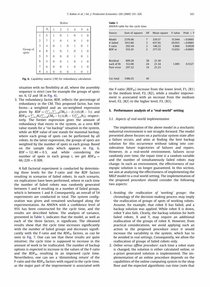

ARTICLE IN PRESS

Robot

Ni 1 2 3 4 5 6

1 5 1 0 1 0 1 0

Group of

2 7 1 0 1 0 1 0

spots

3 4 0 1 0 1 0 1

4 8 1 0 1 0 1 0

5 5 0 0 0 1 0 1

6 5 0 0 1 0 1 0

7 6 0 0 1 0 1 0

8 4 0 0 0 1 0 1

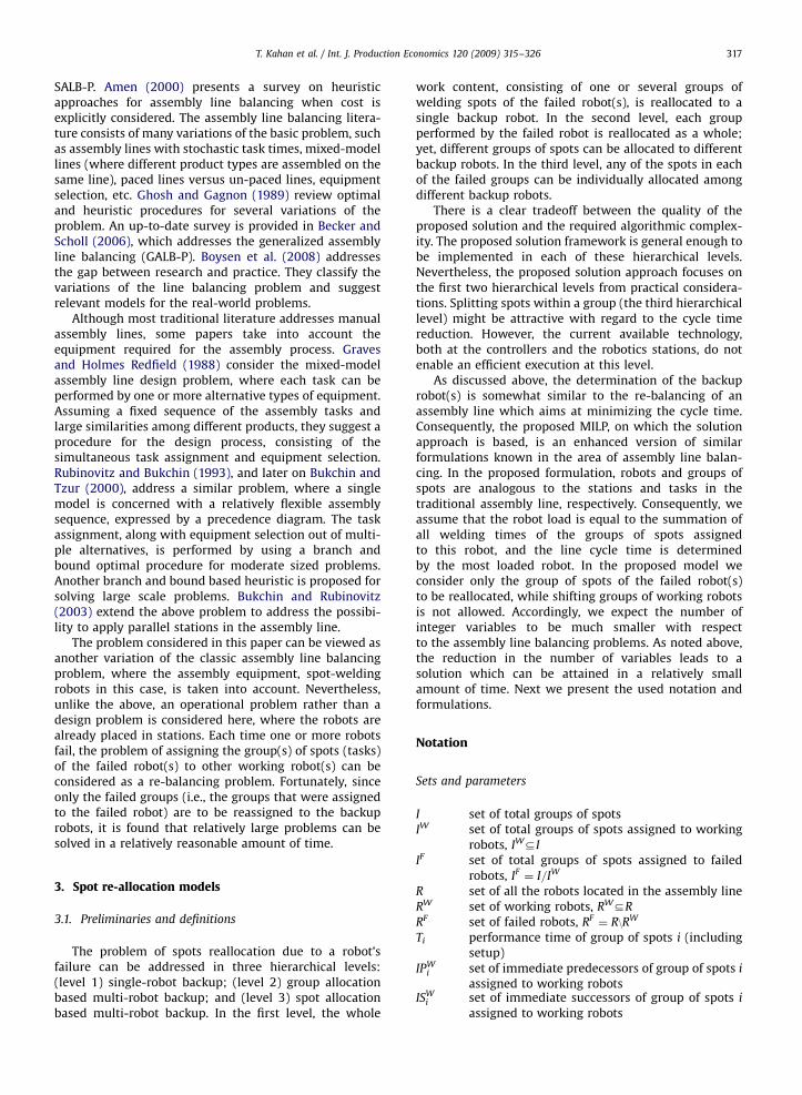
Fig. 6. Capability matrix (CM) for redundancy calculation.

Table 1ANOVA table for the cycle time.

Source Sum of squares DF Mean square F value Prob 4 F

Model 2376.96 7 339.57 15.944 o0.0001

# failed 1913.86 3 637.95 29.955 o0.0001

F-ratio 292.44 2 146.22 6.866 0.0028

RDF w 555.10 2 277.55 13.032 o0.0001

Residual 809.28 38 21.30

Lack of fit 512.06 24 21.34 1.005 0.5127

Pure error 297.22 14 21.23

Cor total 3186.25 45

T. Kahan et al. / Int. J. Production Economics 120 (2009) 315–326 321

situation with no flexibility at all, where the assemblysequence is strict (see for example the groups of spotsno. 6, 12 and 18 in Fig. 4).

3.

The redundancy factor, RDF, reflects the percentage ofredundancy in the CM. This proposed factor, has twoforms—a weighted and an un-weighted expressiongiven by RDF ¼ ð

Pi2I

Pr2RCMirÞ � jIj=ðjIjðjRj � 1ÞÞ and

RDFW¼P

i2INiðP

r2RCMir�1Þ=ððjRj � 1ÞP

i2INiÞ, respect-ively. The former expression gives the amount ofredundancy that exists in the system, as a zero RDFvalue stands for a ‘‘no backup’’ situation in the system,while an RDF value of one stands for maximal backup,where each group of spots can be performed by allrobots. In the latter expression, the groups of spots areweighted by the number of spots in each group. Basedon the sample data which appears in Fig. 6,RDF ¼ 12=40 ¼ 0:3, and while considering thenumber of spots in each group i, we get RDFW ¼

66=220 ¼ 0:309.

A full factorial experiment is conducted by determin-ing three levels for the F-ratio and the RDF factorsresulting in scenarios of failed robots. In each scenario,six replications have been performed, where in each timethe number of failed robots was randomly generatedbetween 1 and 4 resulting in a number of failed groups,which is between 1 and 8. Consequently, an overall of 54experiments are conducted in total. The system config-uration was given and remained unchanged along theexperimentation. An ANOVA with a confidence level of95% has been constructed for the cycle time, and theresults are described below. The analysis of variance,presented in Table 1, indicates that the model, as well aseach of the three factors, is significant. The obtainedresults show that the cycle time increases significantlywith the number of failed groups and decreases signifi-cantly with the F-ratio and the RDFW factors, as can beseen in Fig. 7. One can see that these results are quiteintuitive; the cycle time is supposed to increase in theamount of work to be reallocated. The number of backupoptions is expected to increase in the values of the F-ratioand the RDFW, resulting in an improved cycle time.Nevertheless, one can see a ‘diminishing return’ of theF-ratio and the RDFW factors with regard to the cycle time,as the major part of the improvement is associated with

the F-ratio (RDFW) increase from the lower level, F1, (R1)to the medium level, F2, (R2), while a smaller improve-ment is associated with an increase from the mediumlevel, F2, (R2) to the higher level, F3, (R3).

5. Performance analysis of a ‘‘real-world’’ setting

5.1. Aspects of real-world implementation

The implementation of the above model in a stochasticindustrial environment is not straight-forward. The modelpresented above focuses on a particular system state aftera failure occurs, and aims at finding the best backupsolution for this occurrence without taking into con-sideration future trajectories of failures and repairs.However, in a real-world environment, failures occurrandomly over time, the repair time is a random variableand the number of simultaneously failed robots maychange. In such an environment, the effectiveness of ourmyopic solution is no longer guaranteed. In this section,we aim at analyzing the effectiveness of implementing theMILP model to a real world setting. The implementation ofthe proposed procedure should consider the followingtwo aspects:

1.

Avoiding the reallocation of ‘working’ groups: thechronology of the decision-making process may implythe reallocation of groups of spots of working robots.Assume, for example, that robot X has failed, and abackup solution was applied. While robot X is down,robot Y also fails. Clearly, the backup solution for bothfailed robots, X and Y, may require an additionalreallocation of the groups of robot X. However, frompractical considerations, we avoid applying such anaction in the proposed procedure since it wouldincrease the variability in the system, which has tobe avoided in real settings. Consequently, we allow thereallocation of groups of failed robots only.

2.

Online versus offline procedure: each time a robot stateis changed, the solution is either calculated online, ora-priori generated solution is implemented. The im-plementation of an online procedure depends on thecapabilities of the online computing system in the shopfloor and the expected algorithmic run time (note that

ARTICLE IN PRESS

# Failed

Cyc

le T

ime

One Factor Plot

1 3 7 8

42.00

47.42

52.84

58.27

63.69

F-Ratio

Cyc

le T

ime

One Factor Plot

F1 F2 F3

50.00

52.00

54.00

56.00

58.00

RDFw

Cyc

le T

ime

One Factor Plot

R1 R2 R3

50.00

52.25

54.50

56.75

59.01

Fig. 7. The cycle time versus: the number of failed groups (A); F-ratio (B); and RDFW (C).

T. Kahan et al. / Int. J. Production Economics 120 (2009) 315–326322

experiments resulted in negligible computation timefor real size problems). In a case where the onlineprocedure cannot be implemented, an offline proce-dure is applied instead. In this case, all the solutions ofall possible (or reasonable) scenarios are generated a-priori and stored in the system. As a consequence, eachtime a robot’s state changes, the a-priori generatedsolution is retrieved from the database and implemen-ted. Clearly, the number of possible scenarios dependson the number of robots that can break downsimultaneously. For example, when two out of sixty-five robots can break down simultaneously, thetotal number of failure scenarios is given by

65

1

� �þ

65

2

� �¼ 2;145. This number should be kept

to a relatively small value to enable the implementa-tion of the offline procedure. Another reasonablescenario which may occur in such a stochastic systemis the failure of a robot while another robot is down(rather than a simultaneous fall of two robots). In orderto avoid reallocation of ‘working’ groups (as mayhappen when applying the above solution for twofailed robots), one should generate the solutions ofsuch scenarios in the offline procedure.

The implementation process of the proposed procedureis summarized in Fig. 8. As the system’s state changes,

two options arise. If a failed robot is up again, the originalallocation is resumed, regardless of whether there arecurrently other failed robots. The reason relies on ourassumption that the initial matrix represents the bestwork allocation when all robots are up, and this way,the work allocation of the initial matrix will be resumedeach time the failed robots will be repaired. In casethe change is a result of a newly failed robot, we eitheruse the MILP formulation to generate a backup solution(online procedure) or retrieve the solution from a setof a-priori generated and stored solutions (offline proce-dure). In case such a solution does not exist, the groupsof the newly failed robot are allocated to the MRstation.

5.2. Performance evaluation

Although the proposed formulation can be solved tooptimality, obtaining a global optimum is not guaranteeddue to the stochastic nature of the failures and repairsprocess, which is not taken into account by the MILPformulation. Consequently, the performance of the pro-posed procedure should be validated in a real-worldstochastic environment. To this end, two variations of theproposed procedure are compared with various onlineheuristic allocation rules, by relying on two performancemeasures, cycle time and quality, while the latter is mainly

ARTICLE IN PRESS

System Statehas changed?

Run application/look for a priori

generatedsolution

YES

NO

Feasiblesolutionexists?

YESNOReallocate thefailed robot’s

groups of spots tothe backup robot(s)

Reallocate thefailed robot’s

group of spots tothe MR station

Robot hasfailed?

YES

Failed robot is up -Resume previous

allocation

NO

Update thecurrent robots’

state and groups’allocation

Fig. 8. Backup solution procedure: practical considerations.

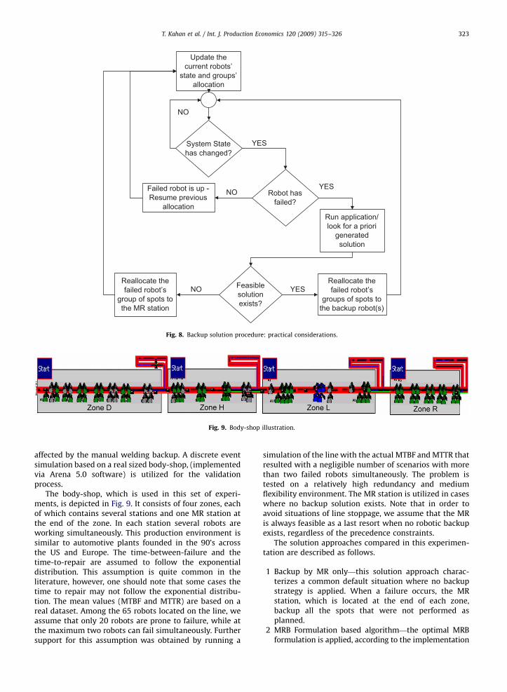
Fig. 9. Body-shop illustration.

T. Kahan et al. / Int. J. Production Economics 120 (2009) 315–326 323

affected by the manual welding backup. A discrete eventsimulation based on a real sized body-shop, (implementedvia Arena 5.0 software) is utilized for the validationprocess.

The body-shop, which is used in this set of experi-ments, is depicted in Fig. 9. It consists of four zones, eachof which contains several stations and one MR station atthe end of the zone. In each station several robots areworking simultaneously. This production environment issimilar to automotive plants founded in the 90’s acrossthe US and Europe. The time-between-failure and thetime-to-repair are assumed to follow the exponentialdistribution. This assumption is quite common in theliterature, however, one should note that some cases thetime to repair may not follow the exponential distribu-tion. The mean values (MTBF and MTTR) are based on areal dataset. Among the 65 robots located on the line, weassume that only 20 robots are prone to failure, while atthe maximum two robots can fail simultaneously. Furthersupport for this assumption was obtained by running a

simulation of the line with the actual MTBF and MTTR thatresulted with a negligible number of scenarios with morethan two failed robots simultaneously. The problem istested on a relatively high redundancy and mediumflexibility environment. The MR station is utilized in caseswhere no backup solution exists. Note that in order toavoid situations of line stoppage, we assume that the MRis always feasible as a last resort when no robotic backupexists, regardless of the precedence constraints.

The solution approaches compared in this experimen-tation are described as follows.

1

Backup by MR only—this solution approach charac-terizes a common default situation where no backupstrategy is applied. When a failure occurs, the MRstation, which is located at the end of each zone,backup all the spots that were not performed asplanned.

2

MRB Formulation based algorithm—the optimal MRBformulation is applied, according to the implementation

ARTICLE IN PRESS

T. Kahan et al. / Int. J. Production Economics 120 (2009) 315–326324

scenarios that were described in Fig. 8. If no solutionhas been found, the groups are allocated to the MRstation.

3

MRB downstream formulation based algorithm(MRBD)—the MRBD is a variation of the MRB formula-tion, in which a backup robot is searched for onlyamong downstream stations. If no solution down-stream has been found, the groups are allocated to theMR station. The motivation behind this approach is todecrease the use of manual stations which havenegative effect on the product’s quality, as well as thecycle time (downstream stations are preferred sincethey can backup the entire failed groups since the timeof the failure. In comparison, upstream backup requiresa manual backup for all the bodies that are betweenthe backup station and the failed station at the time ofthe failure).

4

Heuristic allocation rules—the following heuristics arestate-dependent in nature, by which the backup robotsare chosen online. Each time a robot fails, a feasible setof backup robots (candidates) is obtained taking intoconsideration the precedence constraint and the CM.The reallocation of groups is performed in a descend-ing order of process times, namely, the group with thehighest process time is reallocated first, the one withthe second highest time is reallocated next, etc. If theset of feasible robots is empty, the groups of spots willbe sent to the MR station. The backup robot is selectedbased on one of the following rules:4.1 Nearest capable robot (NCR)—the nearest capable

robot is selected to perform the failing groups ofspots. This heuristic approach searches first for adownstream candidate and only then, if such arobot does not exist, it searches for an upstreamcandidate.

4.2 Most reliable/least loaded robot (RLR)—this rulecombines two characteristics of each robot: itsreliability, defined by its MTBF, and its currentload. Clearly, a robot with higher MTBF and lowercurrent load is preferred for serving as a backuprobot. The weighted sum of these measures, RLRr, iscalculated for each capable robot, r:

RLRr ¼ a1 �MTBFrP

r2RCiðtÞMTBFr

" #

þ a2 �

1pr ðtÞP

r2RCiðtÞ1

pr ðtÞ

" #; 8r 2 RCiðtÞ; 8i 2 IF

where RCi(t) is the set of robots capable ofperforming group of spots i at time t; MTBFr isthe mean time between failures of robot r; pr(t) isthe process time already allocated to robot r attime t; and a1 (a2) is the weight of the reliabilitymeasure (load measure). Note that the values ofthe two measures are normalized between zeroand one for scaling purposes. The closest candidateserves as a tie breaker in this rule. In thisexperiment three rule combinations were chosen,defined by three different weights combinations:(a1,a2) ¼ (0.5, 0.5), (1,0) or (0,1).

4.3 Random capable robot (RCR)—the backup robot israndomly chosen out of the set of possiblecandidates RCi(t).

As noted above, the two performance measures con-sidered here are the cycle time and the quality. The qualitymeasure is associated with the percentage of groups offailed robots that are backed up in the MR station. Thereason is that the quality of spots performed by robots ismuch higher than those that were performed manually,and hence, one prefers to minimize the use of theMR stations. Moreover, the MR also has a negative effecton the cycle time, since the performance time in themanual station is about three times higher than therobotic time.

5.3. Simulation results

A comparison of the commonly implemented backuppolicy (‘‘MR only’’), the MRB, the MRBD and the fiveproposed heuristics (NRC, three variations of RLR and RCR)involves in total eight different solution approaches forthe reallocation problem. A large scale discrete eventsimulation based on a real body-shop was implementedand analyzed via Arena Software 5.0. Every configurationwas simulated by running 50 replications, each of whichof two eight-hour shifts and a warm-up period of 2 hours(statistics were not collected during this period). Since thecycle time is around 1 minute, each run consists ofapproximately 1,000 cycles. The number of 50 replicationswas large enough to guarantee a relatively tight con-fidence interval, as seen next.

The average cycle time, its standard deviation (amongreplications) and the corresponding half width 95%confidence level were collected from the simulation study.The number of groups reallocated to the MR stations’ andparticularly the percentage of this number with respect tothe total number of reallocated groups, were collected andused to define the quality measure of the line. Thesimulation results are presented in Table 2. One can seethat the MRBD (based on the proposed MILP formulationwhere only downstream backup is allowed) outperformsall other methods in both the cycle time and the qualityperformance measures. These results are statisticallysignificant with a confidence level of 95%. In particular,the MRBD provides an average cycle time of 56.69 s versusa cycle time of 63.21 s of the default situation—areduction of 10.3%. In addition, only 3.2% of the groupswhich require backup are allocated to the MR station.

The MRB is the second best with regard to the cycletime performance, however, significantly inferior to MRBDin this measure. Moreover, it suffers from low qualitygrade due to an extensive usage of the MR station forbackup (49.7%). This is due to the use of upstream backuprobots by the MRB approach. In this case, all the groups ofspots located between the backup robot and the failedrobot at the moment of failure are reallocated to the MRstation. As for the quality measure, we can see thatthe NCR approach is the second best with only 6.3%of the backup groups being allocated to the MR station.

ARTICLE IN PRESS

Table 2Results summary of the experimentation.

MR only MRB MRBD NCR RLR (0.5,0.5) RLR (1,0) RLR (0,1) RCR

Cycle time

Average cycle time 63.21 57.9 56.69 58.32 58.3 58.16 58.34 60

STD cycle time 1.414 1.131 1.202 0.955 1.025 1.025 1.061 1.096

Cycle time half width (95%) 0.4 0.32 0.34 0.27 0.29 0.29 0.3 0.31

Failure data

Groups MR counter 487.5 260.9 16.3 34.2 144.76 86.9 170.46 183.4

Groups backup counter 0 264.1 498.7 506.5 382.14 453.7 357.6 328.6

MR Groups (%) 100.0 49.7 3.2 6.3 27.5 16.1 32.3 35.8

Backup Groups (%) 0.0 50.3 96.8 93.7 72.5 83.9 67.7 64.2

56

57

58

59

60

61

62

63

64

0Groups performed in MR

Cyc

le T

ime

[sec

onds

]

MRB

Backup by

MR only

RCR

RLR{0,1}

RLR{½,½}

RLR{1,0} NCR

MRBD

100 200 300 400 500 600

Fig. 10. Cycle time versus quality measure.

T. Kahan et al. / Int. J. Production Economics 120 (2009) 315–326 325

This result is not surprising since in this approachwe first look for downstream backup and only in caseswhere such a backup is infeasible, an upstream backup isadopted.

Regarding the RLR rules one can see that the cycle timeperformance of these three rules is quite comparable, yet,allocating groups to robots with lower MTBF (RLR(1,0))yields a better quality measure than the other twocombinations. Note that the effect of the MR station onthe cycle time results in a higher cycle time even whenallocating groups to the least loaded robots (RLR(0,1)). Ascould be expected, the RCR is the worst heuristic both interms of its cycle time and its quality measure.

The comparative results are also illustrated in Fig. 10,which shows the values of the two performance measuresfor each allocation method. It is evidently seen that allmethods are dominated by the MRBD. In addition, one cansee that the commonly implemented backup policy,where backup is performed only manually, is fullydominated by all the other policies, and in particular bythe MRBD. Hence, we recommend using the MRBD as thebackup approach.

6. Summary and concluding remarks

In this paper we consider a practical spot weldingreallocation problem due to robots’ failures. Two MILPformulations have been suggested to solve the problemwhere a single robot or multiple robots are chosen as thebackup robot(s). Note that the number of integer variablesis relatively small due to the fact that only the groups ofspots of the failed robots are considered as decisionvariables. Consequently, relatively large real-sized pro-blems can be solved via the proposed formulations.Moreover, although the proposed mathematical modelwas designed for a deterministic environment, which doesnot take into account future failures and repairs of robots,a slight variation of it (the MRBD policy) has been found todominate various other backup policies under stochasticconditions.

Future research may include a generalization of theproposed approach to support a mixed-model environ-ment; a dynamic reallocation model—in order to increasethe system’s robustness; and a comparison between thesuggested approaches and other heuristic allocation rules.

ARTICLE IN PRESS

T. Kahan et al. / Int. J. Production Economics 120 (2009) 315–326326

Another possible direction may be associated withdeveloping a solution approach which allows groupsplitting. In this case, a development of easy to usewelding time estimation tools will be needed.

References

Amen, M., 2000. Heuristic methods for cost-oriented assembly linebalancing: a survey. International Journal on Production Economics68, 1–14.

Baybars, I., 1986. A survey of exact algorithm for the simple assembly linebalancing problem. Management Science 32, 909–932.

Becker, C., Scholl, A., 2006. A survey on problems and methods ingeneralized assembly line balancing. European Journal of Opera-tional Research 168 (3), 694–715.

Boysen, N., Fliedner, M., Scholl, A., 2008. Assembly line balancing: whichmodel to use when? International Journal on Production Economics111, 509–528.

Bukchin, J., Rubinovitz, J., 2003. A weighted approach for assembly linedesign with station paralleling and equipment selection. IIETransactions 35, 73–85.

Bukchin, J., Tzur, M., 2000. Design of flexible assembly line to minimizeequipment cost. IIE Transactions 32, 585–598.

Ghosh, S., Gagnon, R.J., 1989. A comprehensive literature review andanalysis of the design, balancing and scheduling of assemblysystems. International Journal of Production Research 27, 637–670.

Graves, S.C., Holmes Redfield, C., 1988. Equipment selection and taskassignment for multiproduct assembly system design. The Interna-tional Journal of Flexible Manufacturing Systems 1, 31–50.

Karp, R.M., 1972. Reducibility among combinatorial problems. In: Miller,R.E., Thatcher, J.W. (Eds.), Complexity of Computer Computation.Plenum Press, New York, pp. 85–103.

Moon, D.H., Cho, H.I., Kim, H.S., Sunwoo, H., Jung, J.Y., 2006. A case studyof the body shop design in an automotive factory using 3Dsimulation. International Journal of Production Research 44,4121–4135.

Noh, S.D., Hong, S.W., Kim, D.Y., Sohn, S.Y., Hahn, H.S., 2001. Virtualmanufacturing for an automotive company (II)—Construction andoperation of a virtual body shop. IE Interface 14, 127–133.

Rubinovitz, J., Bukchin, J., 1993. RALB—a heuristic algorithm for designand balancing of robotic assembly lines. Annals of the CIRP 42,497–500.

Scholl, A., Becker, C., 2006. State-of-the-art exact and heuristic solutionprocedures for simple assembly line balancing. European Journal ofOperational Research 168 (3), 666–693.

Spieckermann, S., Gutenschwager, K., Heinzel, H., Vob, H., 2000.Simulation-based optimization in the automotive industry—A casestudy on body shop design. Simulation 75, 276–286.