instrumentation and tar measurement systems for a ... · instrumentation and tar measurement...
TRANSCRIPT

INSTRUMENTATION AND TAR MEASUREMENT SYSTEMS FOR A DOWNDRAFT
BIOMASS GASIFIER
by
MING HU
B.S., China Agricultural University, 2007
A THESIS
submitted in partial fulfillment of the requirements for the degree
MASTER OF SCIENCE
Department of Biological and Agricultural Engineering College of Engineering
KANSAS STATE UNIVERSITY Manhattan, Kansas
2009
Approved by:
Major Professor Wenqiao Yuan

Copyright
MING HU
2009

Abstract
Biomass gasification is a promising route utilizing biomass materials to produce fuels and
chemicals. Gas product from the gasification process is so called synthesis gas (or syngas) which
can be further treated or converted to liquid fuels or certain chemicals. Since gasification is a
complex thermochemical conversion process, it is difficult to distinguish the physical conditions
during the gasification stages. And, gasification with different materials can result in different
product yields. The main purpose of this research was to develop a downdraft gasifier system
with a fully-equipped instrumentation system and a well-functioned tar measurement system, to
evaluate temperature, pressure drop, and gas flow rate, and to investigate gasification
performance using different biomass feedstock.
Chromel-Alumel type K thermocouples with a signal-conditioning device were chosen
and installed to monitor the temperature profile inside the gasifier. Protel 99SE was applied to
design the signal conditioning device comprised of several integrated chips, which included AD
595, TS 921, and LM 7812. A National Instruments (NI) USB-6008 data acquisition board was
used as the data-collecting device. As for the pressure, a differential pressure transducer was
applied to complete the measurement. An ISA1932 flow nozzle was installed to measure the gas
flow rate.
Apart from the gaseous products yield in the gasification process, a certain amount of
impurities are also produced, of which tar is one of the main components. Since tar is a critical
issue to be resolved for syngas downstream applications, it is important to determine tar
concentration in syngas. A modified International Energy Agency (IEA) tar measurement
protocol was applied to collect and analyze the tars produced in the downdraft gasifier. Solvent
for tar condensation was acetone, and Soxhlet apparatus was used for tar extraction.
The gasifier along with the instrumentation system and tar measurement method were
tested. Woodchips, Corncobs, and Distiller’s Dried Grains with Solubles (DDGS) were
employed for the experimental study. The gasifier system was capable of utilizing these three
biomass feedstock to produce high percentages of combustible gases. Tar concentrations were
found to be located within a typical range for that of a general downdraft gasifer. Finally, an
energy efficiency analysis of this downdraft gasifer was carried out.

iv
Table of Contents
List of Figures ............................................................................................................................... vii
List of Tables ................................................................................................................................. ix
Acknowledgements ......................................................................................................................... x
CHAPTER 1 - Introduction ............................................................................................................ 1
1.1 Gasification Process .............................................................................................................. 2
1.2 Classification of Gasifiers ..................................................................................................... 5
1.2.1 Updraft ........................................................................................................................... 5
1.2.2 Downdraft ...................................................................................................................... 6
1.2.3 Fluidized Bed ................................................................................................................. 7
1.2.4 Entrained Flow ............................................................................................................... 8
1.2.5 Choren Process ............................................................................................................... 9
1.3 Objectives ........................................................................................................................... 10
CHAPTER 2 - Literature Review ................................................................................................. 11
2.1 Biomass Tar Formation ...................................................................................................... 11
2.1.1 Tar Components ........................................................................................................... 11
2.1.2 Tar Yield as a Function of Gasifier Type .................................................................... 14
2.1.3 Tar Formation under Different Biomass Gasification Conditions ............................... 15
2.2 Tar Measurement Methods ................................................................................................. 17
2.2.1 Cold Trapping Method ................................................................................................. 17
2.2.2 Solid-Phase Adsorption (SPA) Method ....................................................................... 20
2.2.3 Molecular Beam Mass Spectrometer (MBMS) Method .............................................. 20
2.2.4 Solvent-free Method .................................................................................................... 22
2.2.5 Quasi Continuous Tar Quantification Method ............................................................. 23
2.2.6 Laser Spectroscopy Method ......................................................................................... 23
2.3 Summary ............................................................................................................................. 24
CHAPTER 3 - Instrumentation and Tar Measurement Systems .................................................. 26
3.1 Instrumentation system ....................................................................................................... 26
3.1.1 Introduction to the Gasifier Unit .................................................................................. 26

v
3.1.2 DC Power for the Blower (AC to DC Converter) ........................................................ 28
3.1.3 Temperature Measurement .......................................................................................... 30
3.1.4 Pressure Drop and Flow Rate Measurement ................................................................ 34
3.2 Tar measurement system .................................................................................................... 37
3.2.1 Tar Measurement - Sampling ....................................................................................... 37
3.2.2 Tar Measurement - Analysis ........................................................................................ 40
3.3 Summary ............................................................................................................................. 41
CHAPTER 4 - Experimental Study .............................................................................................. 43
4.1 Materials and Methods ........................................................................................................ 43
4.1.1 Biomass Feedstock ....................................................................................................... 43
4.1.2 Gasifier System Operation ........................................................................................... 44
4.1.3 Intake Air Temperature Control ................................................................................... 44
4.1.4 Tar and Syngas Analysis .............................................................................................. 45
4.2 Results and Discussion ....................................................................................................... 47
4.2.1 Gasifier Chamber Temperature Profile ........................................................................ 47
4.2.2 Pressure Drop and Air Flow Rate ................................................................................ 51
4.2.2.1 Biomass Loading Affecting Pressure Drop .......................................................... 52
4.2.2.2 Voltage Affecting Pressure Drop .......................................................................... 54
4.2.2.3 Pressure Drop Variations at Different Locations .................................................. 56
4.2.2.4 Pressure Drop at Outlet II ..................................................................................... 59
4.2.2.5 Pressure Drop of the Flow Nozzle and Syngas Flow Rate ................................... 61
4.2.3 Syngas Composition .................................................................................................... 61
4.2.4 Tar Concentration ........................................................................................................ 61
4.2.5 Gasification Energy Efficiency .................................................................................... 62
4.3 Summary ............................................................................................................................. 64
CHAPTER 5 - Summary .............................................................................................................. 65
CHAPTER 6 - Future Research Recommendations ..................................................................... 66
Appendix A - Operating Manual for Downdraft Biomass Gasifier .............................................. 73
Appendix B - Temperature Calibration Chart for AD595 ............................................................ 75
Appendix C - Data of Temperature Profiles and Pressure Drop .................................................. 76
Appendix D - Data Table for Experiment Documentation ........................................................... 80

vi
Appendix E - DDGS Properties Analysis ..................................................................................... 81
Appendix F - Biomass Properties (Gaur and Reed, 1998) ............................................................ 82
Appendix G - Relative Heating Value of Wood as a Function of Moisture Content ................... 83
Appendix H - Calibration of SRI8610 Gas Chromatograph (GC) ............................................... 84
Appendix I - Calculation of flow rate, syngas density, and energy efficiency ............................. 85
Appendix J - Thermodynamic data used by different companies (unit: MJ/Nm3 ) (IEA, 2001) ... 88

vii
List of Figures
Figure 1.1 Reaction zones in a downdraft gasifier ......................................................................... 3
Figure 1.2 Syngas yields from gasification process (Turare, 2002) ............................................... 5
Figure 1.3 Updraft fixed-bed gasifier (Knoef, 2005) ...................................................................... 6
Figure 1.4 Downdraft fixed-bed gasifier (Knoef, 2005) ................................................................. 7
Figure 1.5 Fluidized bed gasifiers: bubbling (left) and circulating (right) (Knoef, 2005) .............. 8
Figure 1.6 Texaco entrained flow gasifier (NETL online resource, www.netl.doe.gov) ............... 9
Figure 1.7 Choren process (Choren, 2007) ................................................................................... 10
Figure 2.1 Biomass tar formation (Evans and Milne, 1987) ......................................................... 12
Figure 2.2 Tar maturation scheme (Elliott, 1988) ......................................................................... 12
Figure 2.3 Tar yield as a function of the maximum temperature exposure .................................. 13
Figure 2.4 Typical particulate and tar loadings in biomass gasifiers (Baker et al. 1986) ............. 15
Figure 2.5 Tar sampling system setup (Kinoshita et al., 1994) .................................................... 16
Figure 2.6 The normalized EPA method for collecting particulates from combustion stack gases
(EPA 1983) ........................................................................................................................... 18
Figure 2.7 Detectable components typical presented in producer gas with Xenon PID lamp
(BTG, 2008) .......................................................................................................................... 19
Figure 3.1 The downdraft gasifier system and its DC motor ........................................................ 27
Figure 3.2 Schematic of the downdraft fixed-bed gasifier ........................................................... 28
Figure 3.3 Circuit of the rectifier box ........................................................................................... 29
Figure 3.4 The rectifier box .......................................................................................................... 29
Figure 3.5 AD 595 for Type-K Thermocouple conditioning (single power supply) .................... 30
Figure 3.6 Printed Circuit Board (PCB) for Thermocouple signal conditioning .......................... 31
Figure 3.7 Thermocouple signal conditioning and data processing ............................................. 32
Figure 3.8 Actual thermocouple arrangement inside the gasifier. ................................................ 32
Figure 3.9 Maximum flow air heater (Omega Engineering) ........................................................ 33
Figure 3.10 Pressure transducer connection and data processing ................................................. 34
Figure 3.11 Theoretical flow nozzle installation .......................................................................... 35

viii
Figure 3.12 Actual flow nozzle installation .................................................................................. 35
Figure 3.13 Schematic of tar sampling system ............................................................................. 38
Figure 3.14 The NALGENE in-line filter holder installation ....................................................... 39
Figure 3.15 The tar sampling device ............................................................................................. 39
Figure 3.16 Tar analysis ................................................................................................................ 40
Figure 4.1 Biomass feedstock samples (left to right: woodchips, corncobs, and DDGS) ............ 43
Figure 4.2 Tar samples (left, solutions; right, dried) .................................................................... 45
Figure 4.3 Syngas composition analysis using a SRI 8610s GC .................................................. 46
Figure 4.4 PeakSimple for GC data analysis ................................................................................ 46
Figure 4.5 Temperature profile inside the gasifier for woodchips gasification ............................ 48
Figure 4.6 Temperature profile of woodchips gasification after the starting run ......................... 49
Figure 4.7 Temperature profile of corncobs gasification after the starting run ............................ 50
Figure 4.8 Temperature profile of DDGS gasification after the starting run ................................ 51
Figure 4.9 Pressure drop measurement through the gasifier system ............................................ 52
Figure 4.10 Pressure drop comparison at different locations through the gasifier system (power
input = 120 V) ....................................................................................................................... 53
Figure 4.11 Pressure drop comparison at different power inputs (voltages) ................................ 55
Figure 4.12 Pressure drop at different locations across the gasifier system ................................. 58
Figure 4.13 Pressure drop at outlet II for woodchips gasification ................................................ 59
Figure 4.14 Pressure drop at outlet II for corncobs gasification ................................................... 60
Figure 4.15 Pressure drop at outlet II for DDGS gasification ...................................................... 60
Figure 4.16 Energy efficiency for woodchips gasification ........................................................... 63

ix
List of Tables
Table 1.1 Biomass feedstock availability in Kansas ....................................................................... 2
Table 2.1 Chemical components in biomass tars (Milne and Evans, 1998) ................................. 12
Table 2.2 Tar classification (Sousa, 2001; Podgórska, 2006) ....................................................... 14
Table 3.1 Gasifier system specification ........................................................................................ 27
Table 3.2 Thermocouples setup inside the gasifier ....................................................................... 33
Table 4.1 Total carbon contents of three biomass samples .......................................................... 43
Table 4.2 DDGS properties (average values) ............................................................................... 44
Table 4.3 Intake air temperature (ambient air temperature = 4 °C) .............................................. 45
Table 4.4 Pressure drop across the flow nozzle and syngas flow rate .......................................... 61
Table 4.5 Syngas composition ...................................................................................................... 61
Table 4.6 Tar concentration .......................................................................................................... 62
Table 4.7 Calorific values (MJ/Nm3) for syngas components (IEA, 2001) .................................. 63
Table 6.1 Output voltage vs. thermocouple temperature at ambient +25 °C (adapted from AD595
specification, Analog Devices) ............................................................................................. 75
Table 6.2 DDGS gasification ........................................................................................................ 76
Table 6.3 Corncobs gasification ................................................................................................... 77
Table 6.4 Woodchips gasification ................................................................................................. 78
Table 6.5 Pressure drop comparison (unit: inch of water) ............................................................ 79
Table 6.6 Test and analysis log for gasification experiment ........................................................ 80
Table 6.7 DDGS properties (data provided by Land O'Lakes Purina Feed) ............................... 81
Table 6.8 The relative heating value of wood as a function of moisture content ......................... 83
Table 6.9 Calculation of flow rate ................................................................................................ 85
Table 6.10 Calculation of syngas density ..................................................................................... 86
Table 6.11 Calculation of energy efficiency ................................................................................. 87
Table 6.12 Gasification energy efficiency for woodchips ............................................................ 87
x
Acknowledgements
First of all, I would like to express my greatest appreciation to my major professor, Dr.
Wenqiao Yuan, for his academic guidance and support through my two-year graduate study, and
for his sharing wisdom with me both in research and life. Two years of communication makes
me better understand the importance of time management, the meaning of commitment to
research, and the way how I need to carry them out.
I also want to thank all the professors who served as my committee members, Drs. Kirby
Chapman, Keith Hohn, and Donghai Wang. Thanks for taking time reviewing my thesis and the
valuable comments. Especially, I own my many thanks to Dr. Hohn for his allowing me to use
the gas chromatograph equipment in his lab, and Dr. Wang for his sharing his laboratory
facilities. All these made my project go on more smoothly and convenient.
Mr. John Hany from Land O'Lakes Purina Feed shall receive my sincere thanks. I felt
grateful for his providing the distillers’ dried grains with solubles (DDGS) sample and sharing
property data of that.
Gratefulness goes to Mr. Darrell Oard for his always ready for help. He has always been
my role model as a great engineer. Also, I need to mention Ms. Barb Moore and Ms. Edna
Razote. Barb is always there since the first date I was admitted to this department. Thanks to
Edna’s advice on gas sampling which made that part of my project easier.
Thank all the department mates, especially my group members in Yuan’s Lab. It’s been
good memories for the days we shared.
Last but not least, my family – my parents, my grandmother, and my sister. They deserve
my heartfelt thanks. Without them, nothing can be made possible.

1
CHAPTER 1 - Introduction
The history of gasification dates back to the seventeenth century. Since the conception of
the idea, gasification has passed through several phases of development. During the 1840s, the
first commercially used gasifier, which was an updraft style, was built and installed in France.
Gasifiers were then developed for different fuels and industrial power and heat applications
(Quaak et al., 1999). The 1970s brought a renewed interest in the technology for power
generation at small scales due to oil crisis (Stassen and Knoef, 1993). Since then, fuels other
than wood and charcoal have been applied as feedstock materials.
As a century old technology, gasification flourished quite well before and during World
War II. Gasifiers were largely used to power vehicles during that period. Many of the gasoline
and diesel driven vehicles during that period were converted to producer gas driven. The
technology was discontinued soon after World War II, when liquid fuel became easily available.
Today, because of increased fuel prices and environmental concerns, there is a renewed interest
in this century old technology. The use of downdraft gasifiers fueled with wood or charcoal to
power cars, lorries, buses, trains, boats and ships have already proved their worth (Turare, 2002).
Gasification has become a more modern and quite sophisticated technology.
Biomass is a complex mixture of organic compounds and polymers (Graboski and Bain,
1979). The major types of compounds are lignin and carbohydrates (cellulose and hemicellulose)
whose ratios and resulting properties are species dependent. Lignin, the cementing agent for
cellulose, is a complex polymer of phenylpropane units. Cellulose is a polymer formed from
glucose; the hemicellulose polymer is based on hexose and pentose sugars. Basically, biomass
includes wood, crop residues, solid waste, animal wastes, sewage, and waste from food
processing, etc. Agricultural wastes such as cotton stalks, saw dust, nutshells, coconut husks, rice
husks and forestry residues - bark, branches and trunk can be used as feedstock. Theoretically,
almost all kinds of biomass materials with moisture content less than 30% can be gasified,
however, in reality not every biomass fuel can lead to successful gasification (Turare, 2002).
Most of the development work is carried out with common fuels such as coal, charcoal and
wood. The key to a successful design of gasifier is to understand the properties and thermal
behavior of the fuel fed into the gasifier system. It was recognized that fuel properties such as

2
surface area, size, shape as well as moisture content, volatile matter and carbon content affect
gasification performance (McKendry, 2002).
The state of Kansas has abundant biomass resources (Walsh, 1999). Biomass feedstock
availability in the state is shown in Table 1.1. When delivered price is less than $40 per dry ton,
agricultural residues account for the largest percentage of the cumulative biomass quantities in
the state. Urban wood wastes and dedicated energy residues are also in rich availability. Other
biomass materials, such as forest residues, and primary mill residues, are in relatively small
amount. Generally, the cumulative quantities promise an adequate storage for biomass utilization
in Kansas.
Table 1.1 Biomass feedstock availability in Kansas Estimated Annual/Cumulative Biomass Quantities (dry ton/yr), by Delivered Price, KS
< $20/dry ton < $30/dry ton < $40/dry ton < $50/dry ton Forest Residues - 47,000 68,000 88,100
Primary Mill Residues 1,000 9,000 20,000 - Agricultural Residues - 0 8,570,003 8,570,003
Dedicated Energy Residues - 0 2,859,261 11,438,271 Urban Wood Wastes 736,289 1,227,148 1,227,148 1,227,148
Cumulative Biomass Quantities 737,289 1,283,148 12,733,412 21,343,522 Note:
1. Estimates of biomass quantities potentially available in five general categories: forest residues, mill
residues, agricultural residues, urban wood wastes, and dedicated energy crops.
2. Availabilities are sorted by anticipated delivered price (harvesting, transportation).
3. Quantities are cumulative quantities at each price (i.e., quantities at $50/dt include all quantities available
at $40/dt plus quantities available between $40 and $50/dt).
1.1 Gasification Process The essence of a gasification process is the conversion of solid carbon fuels into carbon
monoxide and hydrogen by a complex thermochemical process, as shown in the general formula
below.
Biomass + O2 (or H2O) CO, CO2, H2O, H2, CH4
tar + char + ash
+ other hydrocarbons
HCN + NH3 + HCl + H2
Splitting of a gasifier into strictly separate zones is not realistic, but it is conceptually
essential. Generally, there are four zones in a gasifier, the drying, pyrolysis, combustion and
reduction zones, as illustrated in Figure 1.1 (illustrated in a downdraft model).
S + other sulfur gases

3
Figure 1.1 Reaction zones in a downdraft gasifier
Drying
At temperatures above 100 °C, water (moisture content within the biomass) is removed
and converted into steam. In the drying zone, fuels do not experience any kind of decomposition.
Pyrolysis
Biomass is pyrolyzed under conditions being free from air, namely destructive distillation
or thermal decomposition of biomass. The products of biomass pyrolysis have three states: solid
charcoal, liquid wood tar and pyroligneous liquor, and combustible gas. Pyrolyzing at different
temperatures may produce products with different contents. The higher the temperature is, the
greater the amount of combustible gas and liquids, and the less the amount of solid charcoal. The
reaction is influenced by the chemical composition of biomass fuels and the operating
conditions. Charcoal obtained from pyrolysis zone is further reacted in the reduction zone to
yield syngas. Tar and pyroligneous liquor produced in pyrolysis is a liquid containing more than
200 components, like acetic acid, methanol, acetic aldehyde, acetone, ethyl acetate, etc. These
pyrolysis products can be further reacted in the subsequent reaction zones as well. It is noted that
no matter how a gasifier is built, there will always be a low temperature zone where pyrolysis
takes place, generating condensable hydrocarbons (Turare, 2002).
4
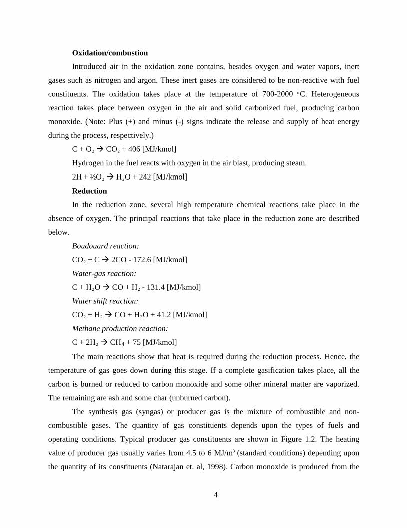
Oxidation/combustion
Introduced air in the oxidation zone contains, besides oxygen and water vapors, inert
gases such as nitrogen and argon. These inert gases are considered to be non-reactive with fuel
constituents. The oxidation takes place at the temperature of 700-2000 °C. Heterogeneous
reaction takes place between oxygen in the air and solid carbonized fuel, producing carbon
monoxide. (Note: Plus (+) and minus (-) signs indicate the release and supply of heat energy
during the process, respectively.)
C + O2 CO2
Hydrogen in the fuel reacts with oxygen in the air blast, producing steam.
+ 406 [MJ/kmol]
2H + ½O2 H2
Reduction
O + 242 [MJ/kmol]
In the reduction zone, several high temperature chemical reactions take place in the
absence of oxygen. The principal reactions that take place in the reduction zone are described
below.
Boudouard reaction:
CO2
Water-gas reaction:
+ C 2CO - 172.6 [MJ/kmol]
C + H2O CO + H2
Water shift reaction:
- 131.4 [MJ/kmol]
CO2 + H2 CO + H2
Methane production reaction:
O + 41.2 [MJ/kmol]
C + 2H2 CH4
The main reactions show that heat is required during the reduction process. Hence, the
temperature of gas goes down during this stage. If a complete gasification takes place, all the
carbon is burned or reduced to carbon monoxide and some other mineral matter are vaporized.
The remaining are ash and some char (unburned carbon).
+ 75 [MJ/kmol]
The synthesis gas (syngas) or producer gas is the mixture of combustible and non-
combustible gases. The quantity of gas constituents depends upon the types of fuels and
operating conditions. Typical producer gas constituents are shown in Figure 1.2. The heating
value of producer gas usually varies from 4.5 to 6 MJ/m3 (standard conditions) depending upon
the quantity of its constituents (Natarajan et. al, 1998). Carbon monoxide is produced from the

5
reduction of carbon dioxide and its quantity varies from 15 to 30% by volume basis. Hydrogen is
also a useful product of the reduction process in the gasifier, which is 10 to 20%. Methane,
carbon monoxide, and hydrogen are responsible for higher heating value of the producer gas.
The amount of methane present in the producer gas is very small. Carbon dioxide and nitrogen
are non-combustible gases in the producer gas. Compared to other gas constituents, nitrogen
presents the highest amount (45 to 60%) in the producer gas. Water vapors in the producer gas
occur due to moisture content of air introduced during oxidation process, injection of steam or
moisture content of biomass fuels.
Figure 1.2 Syngas yields from gasification process (Turare, 2002)
1.2 Classification of Gasifiers A gasifier consists of usually cylindrical chamber with spaces for fuel, air inlet, gas exit,
and grate. It can be made of firebricks, steel, concrete and oil barrels, etc. A complete
gasification system consists of a gasification chamber, purification unit and energy converter – a
burner or internal combustion engine. Based on the design of gasifiers and types of fuels used,
there exists different kinds of gasifiers. Portable gasifiers are mostly used for running vehicles.
Stationary gasifiers combined with engines are widely used in rural areas of developing
countries for many purposes including cooking, heating, generation of electricity and running
irrigation pumps, and so on. The most commonly built gasifiers are classified as:
1.2.1 Updraft The schematic of an updraft gasifier is shown in Figure 1.3. An updraft gasifier has
clearly defined zones for partial combustion, reduction, and pyrolysis. Air is introduced at the

6
bottom and acts as countercurrent to fuel flow. The gas is drawn at a higher location (close to the
top). Updraft gasifiers achieve the highest efficiency as the hot gas passes through the fuel bed
and leaves the gasifier at low temperatures. The sensible heat given by the gas is used to preheat
and dry the fuel. Updraft gasifiers can be easily designed and installed. They are thermally
efficient because the ascending gases pyrolyze and dry the incoming biomass, transferring heat
so that the exiting gases leave very cool. Disadvantages of updraft gas producer are excessive
amount of tar in raw gas (which is due to insufficient heat for cracking the tars) and poor loading
capability since the syngas is also exiting close to the site where biomass is loaded.
Figure 1.3 Updraft fixed-bed gasifier (Knoef, 2005)
1.2.2 Downdraft The schematic of a downdraft gasifier is shown in Figure 1.4. In the updraft gasifier, gas
leaves the gasifier with high tar concentration that may seriously affect the operation of
downstream applications such as internal combustion engines. This problem is minimized in
downdraft gasifier, of which air is introduced into downward flowing packed bed or solid fuels
and gas is drawn off at the bottom. Tars in the raw gas can be cracked or broken down in the heat
reaction zones (i.e., oxidation and reduction) to shorter non-condensable hydrocarbons and
partially converted to syngas. A lower overall efficiency is a common problem in small
downdraft gasifiers because of the heat ‘wasted’ for cracking tars and other heat loss in the
gasification process. Since this type of gasifier has strict requirements on biomass properties

7
(i.e., particles sized between 1 and 30 cm, low ash content, and moisture less than 30%), it has
difficulties in handling higher moisture and ash content fuels. The time needed to ignite and
bring plant to working temperature with good gas quality is shorter than updraft gas producer.
Figure 1.4 Downdraft fixed-bed gasifier (Knoef, 2005)
1.2.3 Fluidized Bed The schematics of fluidized bed gasifiers are shown in Figure 1.5. The operation of the
fixed bed gasifier demands a high fuel quality, particularly a homogenous piece size. Fluidized
bed type gasifiers are more flexible in terms of operation, fuel, scale and the use of gasification
agents. Inert bed material is used (e.g. silica sand) to achieve homogenous conditions and rapid
heat transfer in the fluidized bed. Fluidized bed technique enables long operation periods and
continuous ash removal and bed material renewal. The operation temperature is limited by the
ash (and bed material) sintering temperature below 900 °C. Because tar content depends on
operation temperature, a medium tar and particle laden gas is produced.

8
Figure 1.5 Fluidized bed gasifiers: bubbling (left) and circulating (right) (Knoef, 2005)
1.2.4 Entrained Flow The schematic of an entrained flow gasifier is shown in Figure 1.6. Entrained flow
gasifier needs pulverized fuel and is operated above the ash melting point (>1000 °C). Ash is
removed as liquid phase and due to the high temperature tar content is very low. Two types of
entrained flow gasifiers can be distinguished: slagging and non-slagging. In a slagging gasifier,
the ash forming components melt in the gasifier, flow down the walls of the reactor and finally
leave the reactor as a liquid slag. Generally, the slag mass flow should be at least 6% of the fuel
flow to ensure proper operation. In a non-slagging gasifier, the walls are kept free of slag. This
type of gasifier is suitable for fuels with only little ash.

9
Figure 1.6 Texaco entrained flow gasifier (NETL online resource,
1.2.5 Choren Process
www.netl.doe.gov)
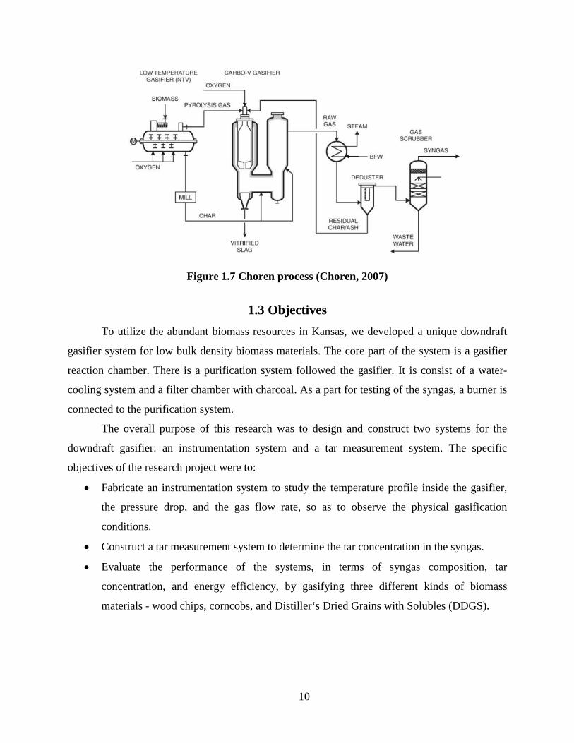
The Choren Company was founded in 1990 by staff of the former East German Deutsche
Brennstoffinstitut with the objective of developing a commercial biomass gasification process as
a basis for manufacturing transport fuels. Choren addresses the tar issue of biomass gasification
by using a three-stage process (Figure 1.7) (Blades et al., 2005). In the first stage, the biomass is
continually carbonized through partial oxidation (low temperature pyrolysis) with air or oxygen
at temperatures between 400 and 500 °C. The pyrolysis gas and char are extracted separately.
The pyrolsis gas is then subjected to high-temperature gasification in the second stage. During
the second stage of the process, the gas containing tar is post-oxidized hypostoichiometrically
using air and/or oxygen in a combustion chamber operating above the melting point of the fuel’s
ash to turn it into a hot gasification medium. During the third stage of the process, the char is
ground down into pulverized fuel and is blown into the hot gasification medium. The pulverized
fuel and the gasification medium react endothermically in the gasification reactor and are
converted into a raw synthesis gas. The Choren process is said to be capable of gasifying a wide
range of feed materials to produce high-quality gas with low tar content and low emission levels.
The capital cost for system construction and operation tend to be higher than other gasifiers.
10
Figure 1.7 Choren process (Choren, 2007)
1.3 Objectives To utilize the abundant biomass resources in Kansas, we developed a unique downdraft
gasifier system for low bulk density biomass materials. The core part of the system is a gasifier
reaction chamber. There is a purification system followed the gasifier. It is consist of a water-
cooling system and a filter chamber with charcoal. As a part for testing of the syngas, a burner is
connected to the purification system.
The overall purpose of this research was to design and construct two systems for the
downdraft gasifier: an instrumentation system and a tar measurement system. The specific
objectives of the research project were to:
• Fabricate an instrumentation system to study the temperature profile inside the gasifier,
the pressure drop, and the gas flow rate, so as to observe the physical gasification
conditions.
• Construct a tar measurement system to determine the tar concentration in the syngas.
• Evaluate the performance of the systems, in terms of syngas composition, tar
concentration, and energy efficiency, by gasifying three different kinds of biomass
materials - wood chips, corncobs, and Distiller‘s Dried Grains with Solubles (DDGS).

11
CHAPTER 2 - Literature Review
2.1 Biomass Tar Formation
2.1.1 Tar Components At an IEA gasification task meeting, it was stated that all organics boiling at temperatures
above that of benzene should be considered as tar (Brussels, 1988). Generally, biomass tar is
referred to condensable organics in the syngas produced in the gasification process of biomass,
and it is assumed to be largely aromatics (Milne and Evans, 1998). Using molecular beam mass
spectrometry (MBMS) suggests a systematic approach to classifying pyrolysis products as
primary, secondary, and tertiary (Evans and Milne, 1987) (Figure 2.1). The primary and tertiary
products are mutually exclusive, that is, the primary products are destroyed before the tertiary
products appear. A commonly used tar maturation scheme, proposed by Elliott (1988), who
reviewed the composition of biomass pyrolysis products and gasifier tar from various conversion
processes, is shown in Figure 2.2. The scheme shows the tar maturation process as a function of
temperature. It indicates the transition as a function of process temperature from primary
products to phenolic compounds to aromatic hydrocarbons. Table 2.1 indicates the classes of
chemical compounds based on GC/MS analysis of collected “tars” (Milne and Evans, 1998).
From this table, tar components varying as temperatures increase is distinguished in each major
regime.

12
Figure 2.1 Biomass tar formation (Evans and Milne, 1987)
Figure 2.2 Tar maturation scheme (Elliott, 1988)
Table 2.1 Chemical components in biomass tars (Milne and Evans, 1998) Conventional Flash Pyrolysis (450–500 °C)
High-Temperature Flash Pyrolysis (600–650 °C)
Conventional Steam Gasification (700–800 °C)
High-Temperature Steam Gasification (900–1000 °C)
Acids Benzenes Naphthalenes Naphthalene* Aldehydes Phenols Acenaphthylenes Acenaphthylene Ketones Catechols Fluorenes Phenanthrene Furans Naphthalenes Phenanthrenes Fluoranthene Alcohols Biphenyls Benzaldehydes Pyrene Complex Oxygenates Phenanthrenes Phenols Acephenanthrylene Phenols Benzofurans Naphthofurans Benzanthracenes Guaiacols Benzaldehydes Benzanthracenes Benzopyrenes Syringols 226 MW PAHs Complex Phenols 276 MW PAHs
From previous research results, it is indicated that temperature is an important factor
affecting tar composition (Baker et al., 1988; Kinoshita et al., 1994; Li et al., 2004; Qin et al.,
2007) showed a conceptual relationship between the yield of tars and the reaction temperature,
shown in Figure 2.3. They cited levels of tar for various reactors with updraft gasifiers having 12
wt% of wood and downdraft less than 1%. For oxygen-blown fluid beds, the levels of tar were
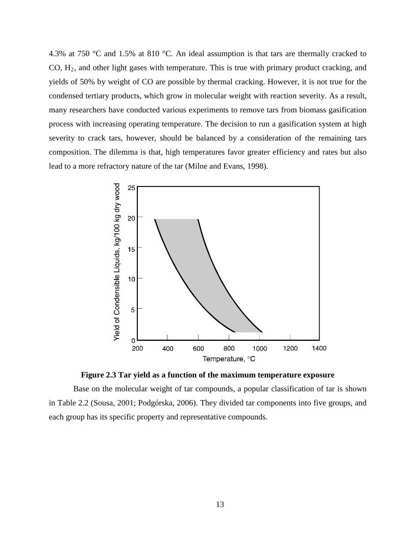
13
4.3% at 750 °C and 1.5% at 810 °C. An ideal assumption is that tars are thermally cracked to
CO, H2, and other light gases with temperature. This is true with primary product cracking, and
yields of 50% by weight of CO are possible by thermal cracking. However, it is not true for the
condensed tertiary products, which grow in molecular weight with reaction severity. As a result,
many researchers have conducted various experiments to remove tars from biomass gasification
process with increasing operating temperature. The decision to run a gasification system at high
severity to crack tars, however, should be balanced by a consideration of the remaining tars
composition. The dilemma is that, high temperatures favor greater efficiency and rates but also
lead to a more refractory nature of the tar (Milne and Evans, 1998).
Figure 2.3 Tar yield as a function of the maximum temperature exposure
Base on the molecular weight of tar compounds, a popular classification of tar is shown
in Table 2.2 (Sousa, 2001; Podgórska, 2006). They divided tar components into five groups, and
each group has its specific property and representative compounds.

14
Table 2.2 Tar classification (Sousa, 2001; Podgórska, 2006)
Tar class Class name Property Representative compounds
1 GC-undetectable Very heavy tars, cannot be detected by GC Determined by subtracting the GC-detectable tar fraction from the total gravimetric tar
2 Heterocyclic aromatics Tars containing hetero atoms; highly water soluble compounds
Pyridine, phenol, cresols, quinoline, isoquinoline, dibenzophenol
3 Light aromatic (1 ring)
Usually light hydrocarbons with single ring; do not pose a problem regarding condensability and solubility Toluene, ethylbenzene, xylenes, styrene
4 Light PAH compounds (2–3 rings)
2 and 3 rings compounds; condense at low temperature even at very low concentration
Indene, naphthalene, methylnaphthalene, biphenyl, acenaphthalene, fluorene, phenanthrene, anthracene
5 Heavy PAH compounds (4–7 rings)
Larger than 3-ring, these components condense at high-temperatures at low concentrations Fluoranthene, pyrene, chrysene, perylene, coronene
Note: GC - gas chromatograph, PAH - polyraromatic hydrocarbon
2.1.2 Tar Yield as a Function of Gasifier Type The amount of tar is a function of the temperature/time history of the particles and gas,
the feed particle size distribution, the gaseous atmosphere, and the method of tar extraction and
analysis. Each type of gasifier has its unique operation and reaction conditions, which results in
different tar composition and yield. Figure 2.4 presents typical tar (note: tar refers to compounds
boiling higher than at 150 °C) and particulate loadings generated in biomass gasifier as reported
by Brown et al. (1986). As a general conclusion, it has been proven and explained scientifically
and technically that updraft gasifiers produce more tars than fluidized beds and fluidized beds
more than downdrafts (Milne and Evans, 1998). In updraft gasifiers, the tar nature is buffered
somewhat by the endothermic pyrolysis in the fresh feed from which the tars primarily arise. In
downdraft gasifiers the severity of final tar cracking is high, due to the conditions used to
achieve a significant degree of char gasification. Tar loading in raw syngas from updraft gasifiers
has an average value of about 100 g/Nm3, fluidized bed and CFBs have an average tar loading of
about 10 g/Nm3, downdraft gasifiers produce the cleanest syngas with tar loading typically less
than 1 g/Nm3. Baker et al. (1986) also concluded very similar research results, which stated a
very general tar level in respect to different gasifier types. It is also established that well-
functioning updraft gasifiers produce a largely primary tar, with some degree of secondary
character; downdraft gasfiers mostly produce tertiary tar, and fluidized beds produce a mixture of
secondary and tertiary tars. Entrained flow gasifiers produce very low level of tar due to the high
temperatures, possible mainly tertiary tar if exists.

15
Figure 2.4 Typical particulate and tar loadings in biomass gasifiers (Baker et al. 1986)
Many publications reported the quantities of tar produced by various types of gasifiers,
under various geometries and operating conditions (Abatzoglou et al. 1997a; Bangala 1997; CRE
Group, Ltd. 1997; Graham and Bain 1993; Hasler et al. 1997; Mukunda et al. 1994a, b;
Nieminen et al. 1996). Tars reported in raw gases for various types of gasifiers is a bewildering
array of values, in each case (updraft, downdraft, and fluidized-bed) spanning two orders of
magnitude. Three of many reasons for this have no relation to the gasifier performance, but are a
result of the different definitions of tar being used, the circumstances of the sampling, and the
treatment of the condensed organics before analysis.
2.1.3 Tar Formation under Different Biomass Gasification Conditions Baker et al. (1988) showed a conceptual relationship between the yield of tars and the
reaction temperature. Li et al. (2004) ran biomass gasification in a circulating fluidized bed, of
which tar yield was measured by in-line tar sampling using a sampling train simplified from the
tar protocol (Knoef, 2000). The experimental data indicated that the tar concentration primarily
depended on the operating temperature. Researchers from the Hawaii Natural Energy Institute
studied how gasification conditions affecting tar formation using a bench-scale indirectly-heated
fluidized bed gasfier (Kinoshita et al., 1994). Three parameters were tested, including
temperature, equivalence ratio, and residence time. Tar samples were collected by a GC with a
flame ionization detector, using a capillary column. Under all conditions tested, tar yield in the

16
product gas ranged from 15 to 65 g/kg biomass, tar concentration ranged from 15 to 86 g/Nm3,
and benzene and naphthalene were the dominant species under most conditions, ranging from 22
to 58% and 4 to 16% of total tars, respectively. Temperature and equivalence ratio have
significant effects on tar yield and tar composition. Lower temperatures favor the formation of
more aromatic tar species with diversified substituent groups, while higher temperatures favor
the formation of fewer aromatic tar species without substituent groups. Their tar sampling system
setup is shown as follows (Figure 2.5). A sintered metal filter removed particulates, and the filter
housing was maintained at 450 oC to prevent condensation of tars in the filter. A slip-stream of
product gas went to the cooling section to condense tars. A water jacket was beyond the sintered
metal filter to condense water vapor in the hot gas. The light fraction of the tars escaping the dry-
ice condenser-trap was removed downstream by two solvent scrubbers connected in series.
Methanol was the solvent used in these two scrubbers.
Figure 2.5 Tar sampling system setup (Kinoshita et al., 1994)
Qin et al. (2007) studied characterization of tar from sawdust gasified in the pressurized
fluidized bed under different operating temperatures and pressures. For pressures of 0.5 to 2.0
MPa, the similar distributions indicated that the pressure had little effect on the molecular weight
distribution of the sawdust air gasified tar under different experimental conditions. The structure
of heavy compounds showed an increase of the aromatic character with the increase in pressure.
The high pressure decreased the devolatilization rate and consequently enhanced the cracking
reactions; the liable bonds could either be dissociated or spontaneously condensed into stable
bonds.
17
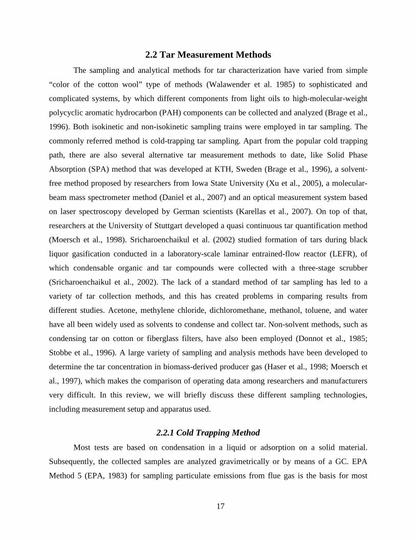
2.2 Tar Measurement Methods The sampling and analytical methods for tar characterization have varied from simple
“color of the cotton wool” type of methods (Walawender et al. 1985) to sophisticated and
complicated systems, by which different components from light oils to high-molecular-weight
polycyclic aromatic hydrocarbon (PAH) components can be collected and analyzed (Brage et al.,
1996). Both isokinetic and non-isokinetic sampling trains were employed in tar sampling. The
commonly referred method is cold-trapping tar sampling. Apart from the popular cold trapping
path, there are also several alternative tar measurement methods to date, like Solid Phase
Absorption (SPA) method that was developed at KTH, Sweden (Brage et al., 1996), a solvent-
free method proposed by researchers from Iowa State University (Xu et al., 2005), a molecular-
beam mass spectrometer method (Daniel et al., 2007) and an optical measurement system based
on laser spectroscopy developed by German scientists (Karellas et al., 2007). On top of that,
researchers at the University of Stuttgart developed a quasi continuous tar quantification method
(Moersch et al., 1998). Sricharoenchaikul et al. (2002) studied formation of tars during black
liquor gasification conducted in a laboratory-scale laminar entrained-flow reactor (LEFR), of
which condensable organic and tar compounds were collected with a three-stage scrubber
(Sricharoenchaikul et al., 2002). The lack of a standard method of tar sampling has led to a
variety of tar collection methods, and this has created problems in comparing results from
different studies. Acetone, methylene chloride, dichloromethane, methanol, toluene, and water
have all been widely used as solvents to condense and collect tar. Non-solvent methods, such as
condensing tar on cotton or fiberglass filters, have also been employed (Donnot et al., 1985;
Stobbe et al., 1996). A large variety of sampling and analysis methods have been developed to
determine the tar concentration in biomass-derived producer gas (Haser et al., 1998; Moersch et
al., 1997), which makes the comparison of operating data among researchers and manufacturers
very difficult. In this review, we will briefly discuss these different sampling technologies,
including measurement setup and apparatus used.
2.2.1 Cold Trapping Method Most tests are based on condensation in a liquid or adsorption on a solid material.
Subsequently, the collected samples are analyzed gravimetrically or by means of a GC. EPA
Method 5 (EPA, 1983) for sampling particulate emissions from flue gas is the basis for most

18
gasifer sampling trains, as shown in Figure 2.6. This method was originally designed for
sampling particulate emissions from combustion flue gases. It was also used to collect gas and
organic liquid samples from stack gases. Modifications have been necessary because of the
higher tar and particulate loadings of gasifier streams. Collected liquids (or, solution) can be
analyzed by high-performance liquid chromatography with UV fluorescence spectroscopy
(Desilets et al., 1984; Corella et al., 1991), size-exclusion chromatography-UV (Adegoroye et
al., 1991), gas chromatography-flame ionization detection (GC-FID) (Brage et al., 1991;
Kinoshita et al., 1994; Blanco et al., 1992), and gas chromatography-mass spectroscopy (GC-
MS) (Bodalo et al., 1994; Padkel and Roy, 1991; Blanco et al., 1991).
Figure 2.6 The normalized EPA method for collecting particulates from combustion stack
gases (EPA 1983)
For isokinetic sampling systems, common elements for measuring the amount of tar and
particulate are a heated filter (glass fiber, cellulose, quartz-fiber, ceramic) for trapping the dust
particles and a condenser for trapping the tar. A general problem of this type of sampling is that
some of the particles collected by the sample filter may have been in gaseous form in the product
gas (BTG, 1995). In addition, some heaviest tar compounds condense on the sample filter and
some create soot particles in the sampling probe. Moreover, some of the heaviest tar compounds
are insoluble in certain solvents or seem to polymerize on the filter paper to form insoluble soot
particles. No clear solution to overcome this problem. Soot forming reactions are probably
19
enhanced by the high temperature, so sampling at lower temperature is recommended. The work
of ETSU/DTI included sampling from different gasifiers (CRE Group, 1997). Authors of that
work undertook as comprehensive as possible identification of tars from various gasifiers. Fresh
sample analysis is recommended to ensure representability of the tar present during the
gasification process. There are a large number of notes on sampling and analysis from the
literature, which presents the diversity of sampling and analysis methods that have been used. A
later project regarding tar sampling and analysis methods has been conducted in BTG ever since
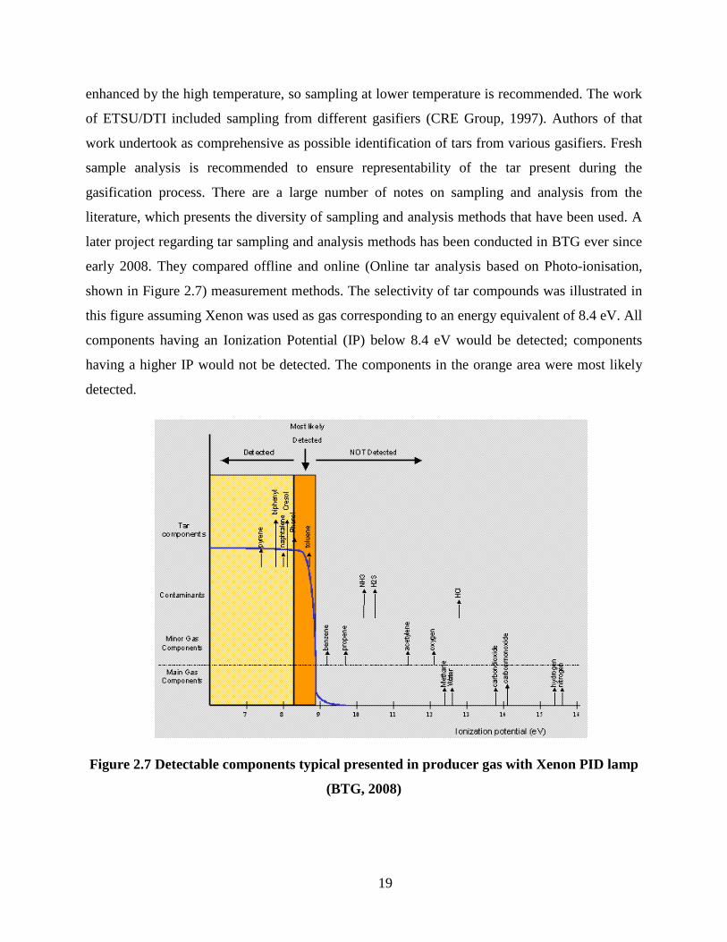
early 2008. They compared offline and online (Online tar analysis based on Photo-ionisation,
shown in Figure 2.7) measurement methods. The selectivity of tar compounds was illustrated in
this figure assuming Xenon was used as gas corresponding to an energy equivalent of 8.4 eV. All
components having an Ionization Potential (IP) below 8.4 eV would be detected; components
having a higher IP would not be detected. The components in the orange area were most likely
detected.
Figure 2.7 Detectable components typical presented in producer gas with Xenon PID lamp
(BTG, 2008)

20
2.2.2 Solid-Phase Adsorption (SPA) Method The solid-phase adsorption (SPA) method is chosen to analyze individual tar compounds
ranging from benzene to coronene, which was originally developed by Royal Institute of
Technology at Sweden (KTH). A gas sample is sucked through an amino-phase sorbent
collecting all tar compounds, then, by using different solvents the aromatic and phenolic
compounds are collected separately and analyzed using a GC. Specifically, in this method
100mL of gas is withdrawn from a sampling line using a syringe or pump for each sample, of
which the sampling line operating temperature is maintained stable at 250-300 °C to minimize
tar condensation. The aromatic fraction is extracted using dichloromethane, and the solution is
analyzed by GC-MS. Afterwards, a second phenolic fraction is eluted using 1:1 (volume ratio)
dichloromethane/acetonitrile. Within this method, a nonpolar capillary column is applied,
focusing on the analysis of mostly non-polar fluidized-bed tars. Given its limits, this method is
applied to measurement of class 2-5 tars (see Table 2.2), which could be fast, simple and reliable
(Osipovs, 2008). The limit of this method lies in, with a high benzene concentration in biomass
tar, some of the benzene are not collected. An improved system added one more adsorbent
cartridge loaded with another sorbent, activated coconut charcoal, which is widely used for
adsorption of volatile organic compounds (including benzene), to the older system. Dufour et al.
(2007) compared the SPA method with the traditional cold trapping method, both methods are
based on GC-MS analysis, when they measured the wood pyrolysis tar, of which they employed
multibed solid-phase adsorbent tubes followed by thermal desorption (SPA/TD) (Dufour et al.,
2007). This new application and comparison proved that SPA/TD is more accurate than
impingers especially for light PAHs.
2.2.3 Molecular Beam Mass Spectrometer (MBMS) Method Evans and Milne (1987) applied molecular-beam, mass spectrometric (MBMS) sampling
method to the elucidation of the molecular pathways in the fast pyrolysis of wood and its
principal isolated constituents. In a follow-up research paper, they also presented the analysis of
effluents from gasification and combustion systems, and found out a full range of products from
the major classes of primary, secondary, and tertiary reactions (Evans and Milne, 1987). Dayton
et al. (1995) from NREL demonstrated the application of MBMS technology to the study of
alkali metal speciation and release during switchgrass combustion. Most recently, researchers
21
from the same lab, NREL, used the same technology to measure gasifier tar concentrations in a
model compound study and during actual biomass gasification, and results were compared to the
traditional method of impinger sampling (Carpenter et al., 2007). A brief description of the
design and operation of MBMS is introduced as follows.
A molecular beam forms as the sampled gases/vapors are drawn through a 300 μm
diameter orifice into the first stage of a three-stage, differentially pumped vacuum system. This
free-jet expansion results in an abrupt transition to collisionless flow that quenches chemical
reactions and inhibits condensation by rapidly decreasing the internal energy of the sampled
gases. The result is that the analyte is preserved in its original state, allowing light gases to be
sampled simultaneously with heavier, condensable, and reactive species. The central core of this
expansion is extracted with a conical skimmer, located at the entrance of the second stage, and
the molecular beam continues into the third stage of the vacuum system. There, components of
the molecular beam are ionized using low-energy electron ionization before passing through the
mass analyzer. From NREL research experience, 22.5 eV allows for sufficient ionization
efficiency while minimizing fragmentation of larger molecules (Carpenter et al., 2007). The ions
are detected with an off-axis electron multiplier, and spectra are generated from the measured
signal intensity as a function of the ion molecular weight. The mass range of interest (up to m/z
(mass-to-charge ratio) 750 with this system) is repeatedly scanned so that the time-resolved
behavior of the system under study can be observed. Because the sample is introduced
continuously by this technique, quantitative measurement of organic and inorganic constituents
in the gasifier process stream can potentially be done once per second. The MBMS system is
equipped with several integrated controls that facilitate sampling of a variety of chemical process
streams. On-board temperature, pressure, and flow control is achieved with I/O control system
interfaced with a PC. Mass flow controllers allow inert gases to be introduced for sample dilution
and internal standards. Liquid standards are injected using two high-pressure liquid
chromatography (HPLC) pumps. Data from each of these auxiliary channels are collected for
subsequent quantitative analysis. The MBMS enables real-time, continuous monitoring over a
large dynamic range [10-6−102% (v/v)]. It can be used to sample directly from harsh
environments, including high-temperature, wet, and particulate-laden gas streams. One limitation
of the MBMS is that there is no pre-separation of the observed peaks. Although fragmentation is
minimized by using low-energy ionizing electrons (22.5 eV), isomers cannot be distinguished,
22
making it difficult to interpret the mass spectra. Complementary analysis, such as impinger
sampling, can be important for initial peak identification.
2.2.4 Solvent-free Method Researchers from Iowa State University designed a so-called dry condenser method (Xu
et al., 2005). It condenses heavy tars (organic compounds with boiling points greater than about
105 °C. Benzene is not treated as a constituent of heavy tar in this context, since its boiling point
is only 80 °C) in a disposable tube and a fiberglass mat. By operating above the boiling point of
water, the heavy tar is not contaminated with moisture. A simple gravimetric analysis of the tube
and fiberglass mat allows the mass of heavy tars to be determined.
The measurement system consists of a heated thimble particulate filter, a dry condenser
constructed from a household pressure cooker, a chilled bottle to condense water and possibly
some light hydrocarbons, a vacuum pump, and a dry gas meter. The dry condenser consists of a
6-m coil of Santoprene tubing and a fiberglass-filled stainless steel canister installed inside the
pressure cooker. The removable lid of the pressure cooker is pierced by compression fittings to
admit gas flow to and from the pressure cooker. Gas entering the pressure cooker flows serially
through the Santoprene tubing and the stainless steel canister before exiting the pressure cooker.
Before sealing the pressure cooker, it is filled with sufficient distilled or deionized water to
submerge the Santoprene tubing and most of the canister. The pressure cooker is placed on an
electric hot plate adjusted to sufficient power to boil water within the pressure cooker. The
pressure cock on the cooker is adjusted to boil water at 105 °C, which prevents water vapor in
the sampled producer gas from condensing inside the Santoprene tubing and on the fiberglass.
Gas exiting the pressure cooker flows through an impinger bottle submerged in an ice bath for
the purpose of removing water (and possibly some light hydrocarbons) from the gas before it
flows through the vacuum pump. A dry gas meter is used to measure total gas flow through the
dry condenser. The pressure and temperature just ahead of the gas meter is recorded periodically
throughout the testing run. Determination of tar is accomplished by measuring the weight change
of the Santoprene tubing and the fiberglass-packed canister before and after a test. When gas
sampling is completed, the Santoprene tubing and fiberglass-filled canister are immediately
removed from the pressure cooker and the outer surfaces wiped dry. The ends of the Santoprene
tubing are sealed, and the tubing is placed in an oven at 105 °C for 1 h, after which its weight

23
change is determined while the canister was immediately weighed. Tar concentration in the
producer gas is calculated by dividing the total weight gain in the tubing and canister by the total
dry gas volume that passed through the dry condenser.
2.2.5 Quasi Continuous Tar Quantification Method Researchers from University of Stuttgart developed a tar quantification method that
allows quasi continuous on-line measurement of the content of condensable hydrocarbons in the
gas from biomass gasification, which makes continuous on-line monitoring possible (Moersch et
al., 2000). The method is based on the comparison of the total hydrocarbon content of the hot gas
and that of the gas with all tars removed. Hydrocarbons are measured with a flame ionization
detector (FID, with high sensitivity and linearity). Tar contents between 200 and 20000 mg/m3
The basic idea of this tar measurement method lies in the comparison of two
measurements. In the first measurement, the total content of hydrocarbons in the gas is
determined. Subsequently all tars are removed by condensation on a filter and a second
measurement is performed to determine the amount of the non-condensable hydrocarbons. The
difference of these two measurements yields the amount of condensable hydrocarbons or tars.
Due to some drawbacks of the measurement system, like influence of the fluctuations of syngas
composition and very small difference of the two measurements when tar contents are too low,
an improved setup was also proposed. Two sample loops are set in the new system, which
guarantees the reference volume for both flows is identical. Both loops are loaded with samples
contemporaneously to remove the fluctuations of the gas concentration. The gas from loop one is
flushed to the FID to determine the total hydrocarbons, while gas from loop two is led to a filter
adsorbing all condensable substances and then passes to the FID yielding the content of non-
condensable hydrocarbons. Analysis time is two minutes with this method (Moersch et al.,
2000).
have been measured reliably.
2.2.6 Laser Spectroscopy Method Researchers from Technische Universität Miinchen in Germany developed a technology
for allothermal gasifier producing hydrogen-rich, high-calorific syngas (Karellas and
Karl, 2007). An optical measurement system based on laser spectroscopy was applied to measure
the basic composition of the product gas and the content of tars in the syngas.

24
Raman spectroscopy has also been used for the analysis of gases. It has been used in
various applications for the investigation of combustion technique (Bombach, 2002). The
quantum theoretical explanation of the Raman effect is: when the incident light quantum hν1
collides with a molecule, it can be scattered either elastically, in which case its energy, and
therefore its frequency, remains unscattered (Rayleigh scattering), or it can be scattered in an
inelastic way (Raman scattering), in which case it either gives up part of its energy to the
scattering system (anti-Stokes scattering) or takes energy from it (Stokes scattering) (Bombach,
2002). The Raman scattering is termed rotational or vibrational depending on the nature of the
energy exchange that occurs between the incident light quanta and the molecules (Herzberg,
1967; Long, 1977). In TUM’s project, an industrial neodium-doped yttrium garnet (Nd:YAG)
laser (Lightwave Electronics) has been used as light source. They used pure gases, and mixed
gases with defined composition for laser system calibration. After measuring the already mixed
gases, they compared the measuring values with already known ones to prove the success of the
calibration process. For the laser spectroscopy method, tars are higher hydrocarbons that emit a
strong fluorescence signal in a wide wavelength range (Bombach, 2002). This signal is detected
as background signal in the profiles when measuring the hot product gas by means of Raman
spectroscopy. With the use of numerical method the background of the signal is approximated
and the area underneath the background profile gives information about the tar content. Different
sampling lines were setup in the measurement system, of which one tar sampling line was
conducted based on IEA method (described as “standardized tar protocol” in the project). The
standardized tar protocol was applied parallel to the laser measurement in order to find the
correlation between the intensity of the optical background signal and tar content. This optical
method could be used to investigate the tar content of the product gas.
2.3 Summary From MBMS study, pyrolysis tar is classified as primary, secondary, and tertiary
products. It is also indicated that tar concentration primarily depends on the operating
temperature. The amount of tar is a function of the temperature/time history of the particles and
gas, the feed particle size distribution, the gaseous atmosphere, and the method of tar extraction
and analysis. Each type of gasifier has its unique operation and reaction conditions, which results
in different tar composition and yield. A general agreement about the relative order of magnitude
25
of tar production is updraft gasifiers being the dirtiest, downdraft the cleanest, and fluidized beds
intermediate.
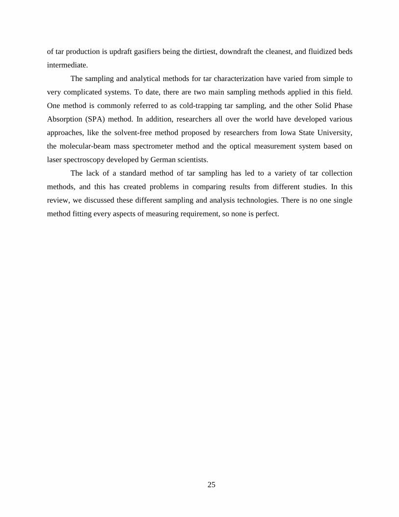
The sampling and analytical methods for tar characterization have varied from simple to
very complicated systems. To date, there are two main sampling methods applied in this field.
One method is commonly referred to as cold-trapping tar sampling, and the other Solid Phase
Absorption (SPA) method. In addition, researchers all over the world have developed various
approaches, like the solvent-free method proposed by researchers from Iowa State University,
the molecular-beam mass spectrometer method and the optical measurement system based on
laser spectroscopy developed by German scientists.
The lack of a standard method of tar sampling has led to a variety of tar collection
methods, and this has created problems in comparing results from different studies. In this
review, we discussed these different sampling and analysis technologies. There is no one single
method fitting every aspects of measuring requirement, so none is perfect.

26
CHAPTER 3 - Instrumentation and Tar Measurement Systems
3.1 Instrumentation system Temperature profile inside the gasifier and pressure drop through the system are proven
to be critical parameters in gasification study. High temperatures are indicators of better carbon
conversion rate, therefore better gasification performance. Pressure drop is closely related to the
fluid flow rate through the gasifier system. Therefore, design and construction of instrumentation
systems is important for a well-monitored gasification process. Accurate measurement of these
data would also provide better control of the system so as to optimize the gasification
performance. Temperature and pressure data are also useful for validation of computational
modeling of gasifiers. For the downdraft gasifier system studied in this project, we designed and
built an AC to DC power transmitter for the blower, a temperature measurement system, a
pressure drop measurement device, and a gas flow rate measurement device.
3.1.1 Introduction to the Gasifier Unit The gasifier, which is shown in Figure 3.1, has an overall syngas production rate of 2.8-
5.6 cfm when coupled with the burner provided. The gasifier system power output is 7-9 HP. A
blower is used to introduce air into the reaction chamber, and syngas output is pumped under the
power of the blower. The pressure of the blower is 1.2 kPa. Power supply for this blower is 80W,
120 VDC (specification shown in Table 3.1). A schematic drawing of the gasifier system is
shown in Figure 3.2. The complete system includes a gasifier chamber, a purification system,
and a burner. Both biomass and gasification medium are introduced through the top, while
syngas exits at the bottom. Through the purification system, the syngas is partially cleaned, and
is burned out after that (except for the part that is collected as samples for analysis).

27
Figure 3.1 The downdraft gasifier system and its DC motor
Table 3.1 Gasifier system specification
Syngas output 2.9-5.8 cfm
Power output 7-9 HP Pressure 1200 Pa Power 80 W
Electric power supply 120 VDC
Applications – From experimental test, this unit can be applied to gasify woodchips easily. Low bulk
density biomass materials, like DDGS and corn stover may be used as feedstock. The producer
gas can be directly burned to supply heat for family or farm use. After careful gas conditioning
and treatment, producer gas from this gasifier can be supplied to the internal combustible engine
for testing, or it may be used as a source for other downstream applications.
Pros and Cons – After setting the unit on a skid, it became portable and convenient for use. Its capability
of utilizing various biomass materials indicated the potential uses in local farms or families
where they have a large amount of agricultural residues.
Tar formation is problematic and may result in operating troubles for the gasifier system.
The accumulated tar within the gasifier can block the pipes or other channels in the gasifier,
which will cause inconvenient syngas production and even some mechanical issues. Regular
cleanup of tars is recommended for this gasifier system. Syngas conditioning is critical if further

28
application of syngas is in consideration, which is technically requiring time and skills. Waste
water is also treated as another environmental problem generated from this unit.
Ste
am
Hea
ter
TC 1
TC 2
TC 3
TC 4
TC 5
TC 6
SP 3
SP 2
SP 1
Stea
m In
ject
ion
Biomass Loading
Air Inlet
Cooling Water Outlet
Cooling Water Inlet
Grate
Ash Disposal
Blower
Drain
Flitrator
TC 6 SP 1
SP 2
Syngas Outlet
Syngas Outlet
Down-draft Gasifier SystemTC – Thermocouple (Type – K)SP – Sampling Port
Figure 3.2 Schematic of the downdraft fixed-bed gasifier
3.1.2 DC Power for the Blower (AC to DC Converter) The intake air is sucked in by a blower. Since the blower is driven by a DC motor, the
wall power (120 VAC) needs to be converted to 120 VDC power. Based on the principle of full-
wave rectifier circuit, a rectifier box was constructed to convert AC to DC in order to power the
blower (Figures 3.3 and 3.4). The rectifier selected permitted a maximum current of 5 amp. A 5
amp fuse was used to protect the circuit.
inlet level

29
AC
DC Output: ~110V
Fuse holder:Fuse - 5 amp maximum
Switch
Rectifier:250V, 5 amp
AC Input:110-120V
Figure 3.3 Circuit of the rectifier box
Figure 3.4 The rectifier box
Materials used to construct the rectifier box included a fuse holder (5 amp maximum),
switch, rectifier (250 V, 5 amp), heat sink, project enclosure, and flexible banana plugs. As
shown in Figure 3.4, the side with banana plugs is DC power output, and the opposite side
accepts the AC power. With the help of a 5 amp variable voltage transformer (All Electronics
Inc), the power input could be adjusted, which affected the DC motor to drive the blower.
Therefore, air blown could be adjusted accordingly in the gasifier system.
30
3.1.3 Temperature Measurement Given the high temperature inside the gasifier, we utilized Chromel-Alumel type K
thermocouples (standard limits of error: ±2.2 °C or 0.75%, whichever is greater; specific limits
of error: ±1.1 °C or 0.4%, whichever is greater) (Omega Engineering) to accomplish the
measurement. It is low cost and, owing to its popularity, it is available in a wide variety of
probes (grounded junctions were chosen in this project). Type K thermocouples are available in
the -200 °C to +1200 °C range. Sensitivity is approximately 41 uV/°C. A thermocouple signal-
conditioning device was also designed and tested. Two main integrated chips (ICs), AD 595
(Analog Devices) and TS 921 (STMicroelectronics), were employed to fabricate the device. The
temperature calibration chart was provided with AD595 specification (Appendix B).
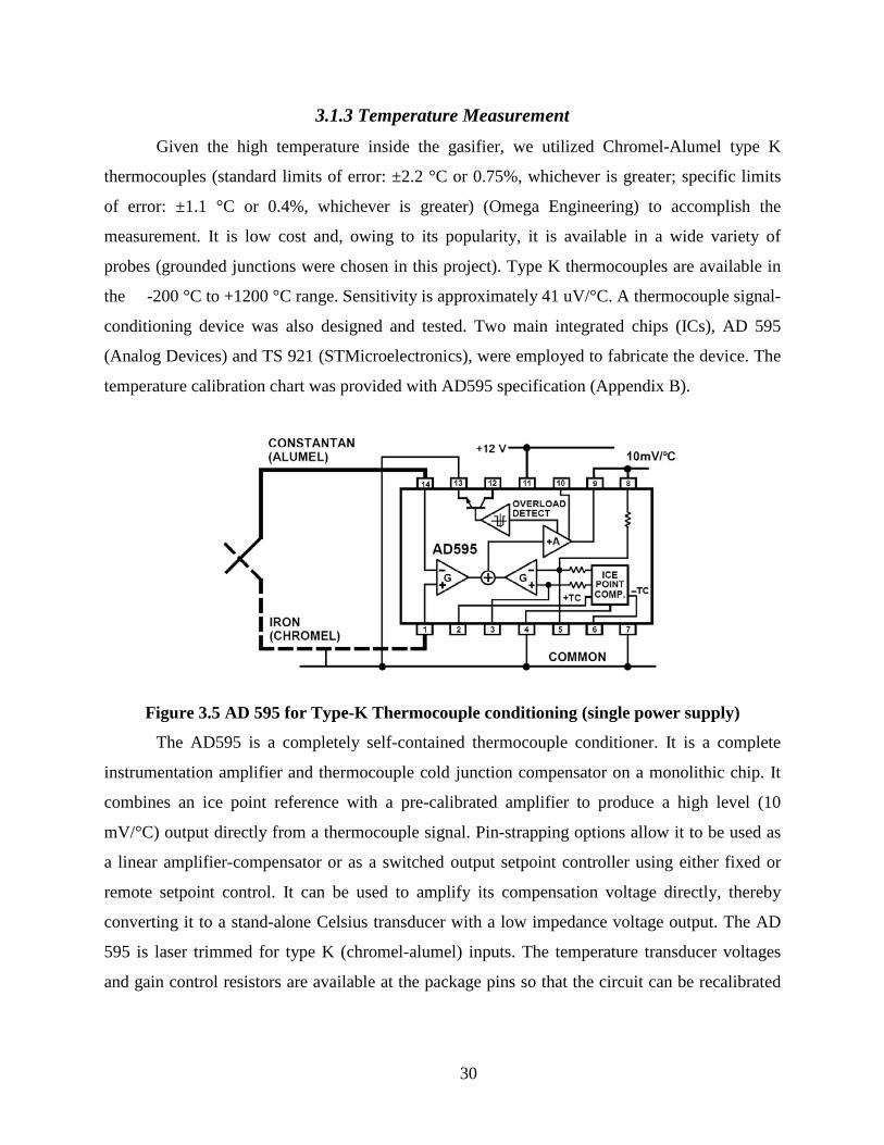
Figure 3.5 AD 595 for Type-K Thermocouple conditioning (single power supply)
The AD595 is a completely self-contained thermocouple conditioner. It is a complete
instrumentation amplifier and thermocouple cold junction compensator on a monolithic chip. It
combines an ice point reference with a pre-calibrated amplifier to produce a high level (10
mV/°C) output directly from a thermocouple signal. Pin-strapping options allow it to be used as
a linear amplifier-compensator or as a switched output setpoint controller using either fixed or
remote setpoint control. It can be used to amplify its compensation voltage directly, thereby
converting it to a stand-alone Celsius transducer with a low impedance voltage output. The AD
595 is laser trimmed for type K (chromel-alumel) inputs. The temperature transducer voltages
and gain control resistors are available at the package pins so that the circuit can be recalibrated

31
for the thermocouple types by the addition of two or three resistors. These terminals also allow
more precise calibration for both thermocouple and thermometer applications.
Using a single +12 V supply, the interconnections shown in Figure 3.5 provided a direct
output from a type K thermocouple (AD 595) measuring from 0 °C to +1200 °C. Any convenient
supply voltage from +5 V to +30 V may be used, with self-heating errors being minimized at
lower supply levels. In the single supply configuration, the +12 V supply connects to Pin 11 with
the V– connection at Pin 7 strapped to power and signal common at Pin 4. The thermocouple
wire inputs were connected to Pins 1 and 14 either directly from the measuring point or through
intervening connections of similar thermocouple wire type. The alarm output at Pin 13 was not
used but connected to common or –V. The pre-calibrated feedback network at Pin 8 was tied to
the output at Pin 9 to provide a 10 mV/°C nominal temperature transfer characteristic.
The TS921 is a RAIL TO RAIL single BiCMOS operational amplifier with low noise and
low distortion. Since the output voltage from AD 595 could not be detected by the data
acquisition system, the TS921 was applied as a signal delivery (buffer) using a negative feedback
which would simply follow the input voltage (from AD 595) with a stable gain of 1.
Figure 3.6 Printed Circuit Board (PCB) for Thermocouple signal conditioning

32
Figure 3.7 Thermocouple signal conditioning and data processing
As shown in Figure 3.6, Protel 99 SE was used to design the PCB board, which included
8 parallel type K thermocouple signal conditioning circuits. In Figure 3.7, it indicated the
working condition of the temperature measurement device, which included a 24 VDC power
supply (Omega Engineering Inc.), a NI USB-6008 data acquisition board, and the temperature
measurement box. It is noted that a DC voltage regulator, LM 7812 (National Semiconductor
Corporation), was used to convert the 24 VDC to 12 VDC so as to supply power for the ICs.
Figure 3.8 Actual thermocouple arrangement inside the gasifier.

33
In order to monitor the temperature profiles at different reaction zones inside the gasifier,
a series of type K thermocouples were set to accomplish this task. Thermocouples were set along
the gasifier wall in different locations, as shown in Figure 3.8. The first thermocouple was set to
measure the intake air temperature. The intake air temperature was controlled by a high-flow-rate
heater (Omega Engineering Inc.) which can be manually adjusted by power supply or air flow
rate (Figure 3.9). This air heater was designed with a 60 mm (outsider diameter) aluminum tube
and a cross frame heating element for minimum resistance to air flow. A 102 mm round flange
with pre-drilled holes at the inlet side were used for mounting the heater. This heater had a
practical operating range of up to 200 CFM with temperatures up to 315 °C.
Figure 3.9 Maximum flow air heater (Omega Engineering)
As shown in Table 3.2, the other four thermocouples were set accordingly to a theoretical
reaction zone distribution inside a typical downdraft gasifier (Knoef, 2005). They were placed at
18-inch, 12-inch, 5-inch, (all heights related to the grate), and the grate, to estimate temperatures
at different reaction zones.
Table 3.2 Thermocouples setup inside the gasifier Port TC Code Approximate reaction zone Inlet TC0 N/A
18 inches from the grate TC1 Drying 12 inches from the grate TC2 Pyrolysis 5 inches from the grate TC3 Oxidation
The grate TC4 Reduction Exit TC5 N/A

34
3.1.4 Pressure Drop and Flow Rate Measurement In this study, a differential pressure transducer (type: PX274-30DI; accuracy: ±1.0% FS)
(Omega Engineering Inc.) was applied to evaluate the pressure change across the gasifier, also
that of the flow nozzle. The transducer was pre-calibrated by the manufacture. It was calibrated
to deliver 4-20 mA corresponding to a pressure range of 0-30 inches of water, linearly. The USB
6008 board is set up to receive voltage. Therefore, a resistor across the input terminals of the
instrumentation was installed to solve this problem. The value of the resistor was determined by
Ohms law (V = IR). The connection of the pressure transducer to the data acquisition board was
completed using a 470 ohm resistance in series with the transducer (Figure 3.11).
Power supply
Pressure transducer
DAQ board
4-20mA loop R
Figure 3.10 Pressure transducer connection and data processing
Measurement of fluid flows in pipes is commonly implemented using orifice, nozzle, and
venturi. The air flow rate measurement using nozzle is proven to be precise, but proper
installation is critical. Therefore, a flow nozzle (i.e., ISA1932 nozzle) with a throat diameter of 1
inch and straight PVC pipe of 2 in (Diameter Ratio, β=d/D=0.5) were chosen to accomplish this
measurement. The part of the nozzle inside the pipe is circular. The nozzle consists of a
convergent section, rounded profile, and a cylindrical throat. Design and manufacture of the flow
nozzle are based on the standard and specification. Pressure taps were set 2 inches ahead of the
nozzle and 1inch behind it, respectively (distances were based on the upstream face of the
nozzle). The minimum upstream and downstream straight lengths were 6 inches and 5 inches,
respectively. Construction was completed according to an ASME standard (ASME, 2004). As
indicated in following figures, Figure 3.11 is the theoretical installation of flow nozzle, and
Figure 3.12 shows the actual construction. For experimental operation, it was connected to the

35
syngas outlet so as to test the pressure drop between the two pressure taps, during the actual
working condition.
Figure 3.11 Theoretical flow nozzle installation
Figure 3.12 Actual flow nozzle installation
The mass flow rate (qm) and volume flow rate (qv
4
12
1
24 β
ρεπ−
∆=
pCdqm
) are related to the differential pressure,
and both are computed by the following equation (SI Units) (ASME, 2004):
ρm
vqq =
15.16
15.421.4 )10)(0033.000175.0(2262.09900.0DR
C βββ −−−=
( ) 5.0/1
/24
4/2
11
11
1
−
−
−−
−
=−
ττ
τββ
κκτε
κκ
κ
κ
Where,
C is the discharge coefficient;
ε is the expansibility factor;
36
∆p is the differential pressure (p1-p2), p1 refers to high pressure at upstream, and p2
ρ
refers to low pressure at downstream (Pa);
1 is the density of the fluid at the upstream pressure tap (kg/m3
ρ is the fluid density at the temperature and pressure for which the volume is stated
(kg/m
);
3
β is the diameter ratio;
);
RD
τ
is the Reynolds number referred to D;
is the pressure ratio (p2/p1
κ
);
is the isentropic exponent (its value depends on the nature of the gas).
Both values for C and ε can be looked up in the appendix forms at the ASME standard
(ASME, 2004). Uncertainties of flow rate measurement includes three parts, that of discharge
coefficient C (equals to ±0.8%), that of expansibility factor ε (equals to ±2∆p/p2
pCC
CC∆
+−−
−−−224
224
)1(1
)1(1
ββ
ββ
%), and that of
pressure loss ∆w (∆w = ).
Calculation of flow rate was completed in a 2003 Microsoft Excel spreadsheet (Table 6.9,
Appendix I). The known parameters for flow rate calculation were d and β. In addition, ∆P and
P1 were measured using the differential pressure transducer under working conditions. The other
unknowns needed to be estimated or computed as follows. Firstly, discharge coefficient and
expansibility factor, C and ε, could be looked up in the tables of discharge coefficients and
expansibility factors (Appendix J). From the pressure measurement, P2/P1 was 0.999 (therefore
ε=1). A first guess of RD was made in an iterative computation, and the corresponding C was
obtained. Under the first guess, a tentative result of flow rate was obtained. Given this flow rate,
the syngas velocity in the pipe was resulted; and given this velocity, the Reynolds number was
computed. Compare this number with the guessed number. When they were closest to each
other, it was treated as the final guess. The final value for C was 0.9758 (RD
Another parameter needed to be calculated to find flow rate was the syngas density at the
temperature and pressure for which the volume was stated. The temperature at outlet II was
measured using a thermocouple. It was 49 °C on average. Since pressure drop was very small
compared to atmosphere pressure, the pressure at outlet II was treated as 1atm. Syngas density
was computed based on the ideal gas law, as indicated in Table 6.10 (Appendix I). Gas density
for each component was computed. The density for gas mixture was calculated based on the
=300,000).

37
percentage and density of each component. The syngas (of woodchips gasification) density at 49
°C, 1atm was 0.8679 kg/m3
3.2 Tar measurement system
.
The main impurities in the syngas of biomass gasification are tar and particulate.
Effective and accurate measurement techniques allow determination of the efficiency of the
syngas cleaning process and ensure the quality of the cleaned gas to be used in downstream
applications, like engines or turbines.
As reviewed in Chapter 2, various sampling and analysis methods have been developed
to determine tar concentration in syngas. This makes the comparison of operational data difficult
and represents a significant barrier to further development. Compared to other methods, cold
trapping method is relatively simple in principle. The system is inexpensive and easy to build.
Therefore, this route was chosen as the model for design and construction.
In this study, a modified International Energy Agency (IEA) method was used to measure
the tar and particulate concentration. The measurement principle is based on sampling of a gas
stream containing tars and particulates driven by a vacuum pump. The test method is carried out
in two steps: sampling and analysis.
3.2.1 Tar Measurement - Sampling As shown in Figure 3.13, the sampling system consists of a filter holder containing fiber
glass filter paper, a series of 6 sampling bottles (250 ml) containing acetone (100 ml each), and
air flow meter. The sampling bottles were placed in the warm (40 °C ±1 °C, controlled by adding
hot water if readings of the thermometer decrease) and cold bath (0 °C controlled by ice) to
collect tars which were condensed in the solvent. The two different bathes were set for staged
warming and cooling of the sampled gas. Syngas was sampled for a specific period (15 minutes)
through the sampling line and filter. The sampling rate was constant, about 9-10 L/min, which
was maintained with the aid of a vacuum pump. After sampling, the content of the sampling
bottles was decanted into a large bottle for later analysis. All sampling bottles and sampling
tubes were rinsed using acetone to collect residue tars and particulates.

38
1 2 34 5 6Warm Bath,
40oCCold Bath,
0oC
Sampling Bottles
Air Flow Meter
Vacuum Pump
Filter HolderFilter Paper
Sampling Port
(Part of the purifier
chamber)
Figure 3.13 Schematic of tar sampling system
It is noted that, both warm bath and cold bath were used in the sampling line, the
temperature of sampling bottles 1, 2, and 4 is 40 °C, the temperature of 3, 5, and 6 is 0 °C. The
temperature gradient benefited the condensation of tar in acetone. Acetone was the solvent that
was used to condense tars. Before using the equipment in connection with a site measurement,
all glass equipment was cleaned in three steps. (1) Pre-washing (2) Wash all glassware in hot
soapy water using a suitable bottlebrush to clean the internal parts of the glassware. Any
glassware that was stained should be soaked for 4 hours, and then rinsed ten times before
washing it with soapy water. (3) All glassware should be rinsed three times in tap water, three
times in double-distilled water, dried, and stored in a clean place. (Cleaned glassware should be
inspected, dried at 150 °C in a drying oven, capped with aluminum foil, and stored in a closed
cabinet.)
Materials used to construct the sampling device included the following parts: vacuum
pump (Thermo Scientific), glass fibre filter paper (Fisher Science, AP 40) , Thimble filter (25
mm×80 mm) (Whatman), filter holder (NALGENE, as indicated in Figure 3.14), and air flow
meter (Dwyer Instruments). The final working condition of the sampling system is indicated in
Figure 3.15.
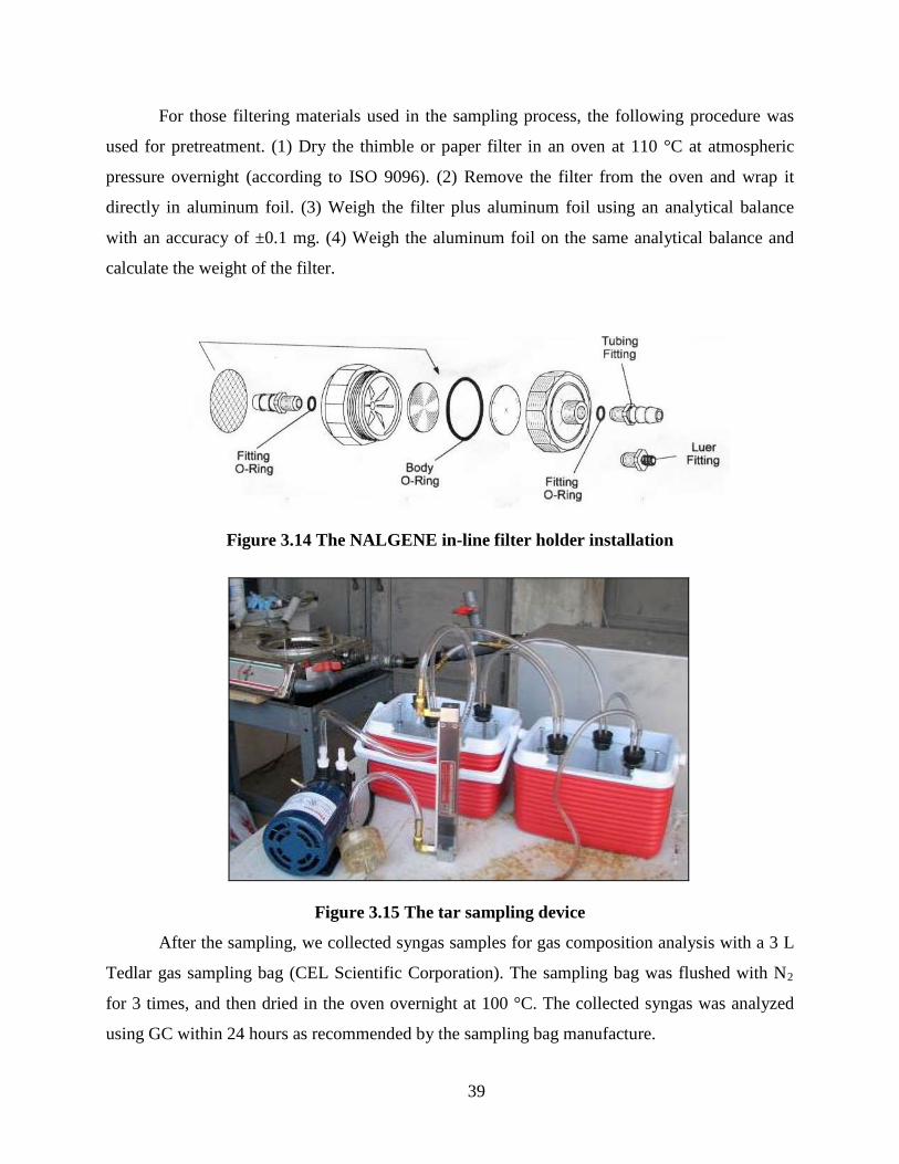
39
For those filtering materials used in the sampling process, the following procedure was
used for pretreatment. (1) Dry the thimble or paper filter in an oven at 110 °C at atmospheric
pressure overnight (according to ISO 9096). (2) Remove the filter from the oven and wrap it
directly in aluminum foil. (3) Weigh the filter plus aluminum foil using an analytical balance
with an accuracy of ±0.1 mg. (4) Weigh the aluminum foil on the same analytical balance and
calculate the weight of the filter.
Figure 3.14 The NALGENE in-line filter holder installation
Figure 3.15 The tar sampling device
After the sampling, we collected syngas samples for gas composition analysis with a 3 L
Tedlar gas sampling bag (CEL Scientific Corporation). The sampling bag was flushed with N2
for 3 times, and then dried in the oven overnight at 100 °C. The collected syngas was analyzed
using GC within 24 hours as recommended by the sampling bag manufacture.

40
3.2.2 Tar Measurement - Analysis Tar sampling started once the gasification approached stable condition which was
indicated by the burner flame. This process took 15 minutes to finish. The fiber glass filter paper
containing particulate sample was Soxhlet extracted in order to remove adsorbed tar.
Subsequently the amount of particulate was determined gravimetrically. Equipment for
gravimetric analysis included Soxhlet apparatus (Figure 3.16), evaporator, analytical balance,
and laboratory equipment as volumetric flasks. The tars from the Soxhlet extraction were added
to the liquid tar samples. The liquid sample containing tars was evaporated under certain
conditions (i.e., heater temperature was set at 80 °C).
To avoid polymerisation of tar this procedure was undertaken immediately after finishing
the sampling. First, open the filter housing and transfer the thimble filter to the Soxhlet
apparatus. Keep it in the vertical position to avoid loss of particles. Carefully add the appropriate
amount (250-500 ml) of acetone to the Soxhlet apparatus. Extract the filter until the acetone was
clear. And then, remove the filter from the Soxhlet and keep it in the vertical position. Finally,
both the filter paper and filter thimble were dried at 110 °C at atmospheric pressure overnight.
wash(acetone)
Sampling bottle
Distillation bottle
Thimble filter
Soxhlet Apparatus
Use the recycled acetone to wash the
sampling bottle (each for once)
Oven
Dry (49
O C, 12 h
r)
Oven
Dry (49 OC, 12 hr) After distillation
Figure 3.16 Tar analysis
41
Analysis procedure goes as follows. First, wash the sampling line (stainless pipes and
hoses) along the syngas flow direction, collect the acetone mixture in one of the sampling
bottles. Use the thimble filter to collect the particulates contained in the acetone mixture, and set
up the Soxhlet apparatus in the lab to extract tar. After 5 hours’ continuous extraction, remove
the thimble from the Soxhlet chamber, dry them (thimble + filter paper) in the oven at 105 °C for
2 hours. Finally, use mass gravimetric method to compute weights of tar and particulate.
Appropriate handling of the leftovers is a must to avoid safety issues. Wash all the flasks
and bottles with solvents (acetone and/or ethanol) timely, and dry them in the oven to remove
possible residues inside the flasks or bottles.
3.3 Summary As a thermo-chemical conversion process, biomass gasification experiences significant
temperature and pressure variations. For the purpose of successful operation of the gasifier
system, it is necessary to accurately measure and monitor the changes of these parameters. In this
study, three different instrumentation systems, including temperature measurement, differential
pressure estimate, and fluid flow rate calculation, were designed and constructed. On top of that,
a full-wave rectifier circuit was applied to convert the AC power to DC power, plus the
regulation of AC input via a variable voltage transformer. These devices could be applied to
control the intake air temperature by manually varying the input voltage via the variable voltage
transformer, monitor the temperature variations inside the gasifier, investigate the pressure drop
through the operation system, and calculate the syngas flow rate. The estimation of these
parameters benefited the suitable operation of the gasifier system and could be used as useful
information to improve the biomass gasification performance. These instrumentation systems
were either calibrated or pre-calibrated, and they were tested in the experimental study and
proven to be accurate and stable, which will be discussed in details in Chapter 4.
In order to determine tar and particulate concentrations in the syngas of biomass
gasification, a tar sampling method based on the IEA tar protocol was developed. As a two-step
measurement system, both sampling and analysis procedures were carefully manipulated.
Preliminary test of this measurement system indicated that the particulate concentration was too
low to be estimated. This may due to the gas conditioning in the purifier system, which reduced
the amount of particulate to a very low level. Therefore, in the experimental test, we assumed

42
that ideally there was zero concentration of particulate and tar measurement system only
included tar concentration determination function. As stated and explained in Chapter 4, this
study proved the effectiveness of the tar measurement system, and the tar concentration was
typical as that of downdraft biomass gasifier indicated in the literature.

43
CHAPTER 4 - Experimental Study
In order to test the instrumentation and tar measurement systems as well as the gasifier,
several experimental tests were conducted with three different biomass materials as feedstock,
including woodchips, corncobs, and DDGS. In this part, the experimental results, such as
temperature profiles inside the gasifier, pressure drop, syngas flow rate, tar concentration, syngas
composition, and energy efficiency, will be discussed.
4.1 Materials and Methods
4.1.1 Biomass Feedstock Wood chips (City transfer center, Manhattan, KS), Corncobs (Kaytee Products Inc.,
Chilton, WI), and DDGS (Land O’Lakes Purina Feed, Shoreview, MN) were used as feedstock
(Figure 4.1).
Figure 4.1 Biomass feedstock samples (left to right: woodchips, corncobs, and DDGS)
Carbon content for each feedstock was tested in the Soil Testing Laboratory at Kansas
State University (Table 4.1). It was indicated from the test, that these three biomass materials
generally have similar amount of carbon content, all in the range of 43-44%. For DDGS, the
supplier also provided a table of various properties (Table 4.2). It mainly included moisture,
protein, fat, total starch, etc.
Table 4.1 Total carbon contents of three biomass samples
Sample ID Total N % Total C % wood chips - 1 0.24 44.26
DDGS - 2 3.78 43.25 corn cobs - 3 0.31 44.66
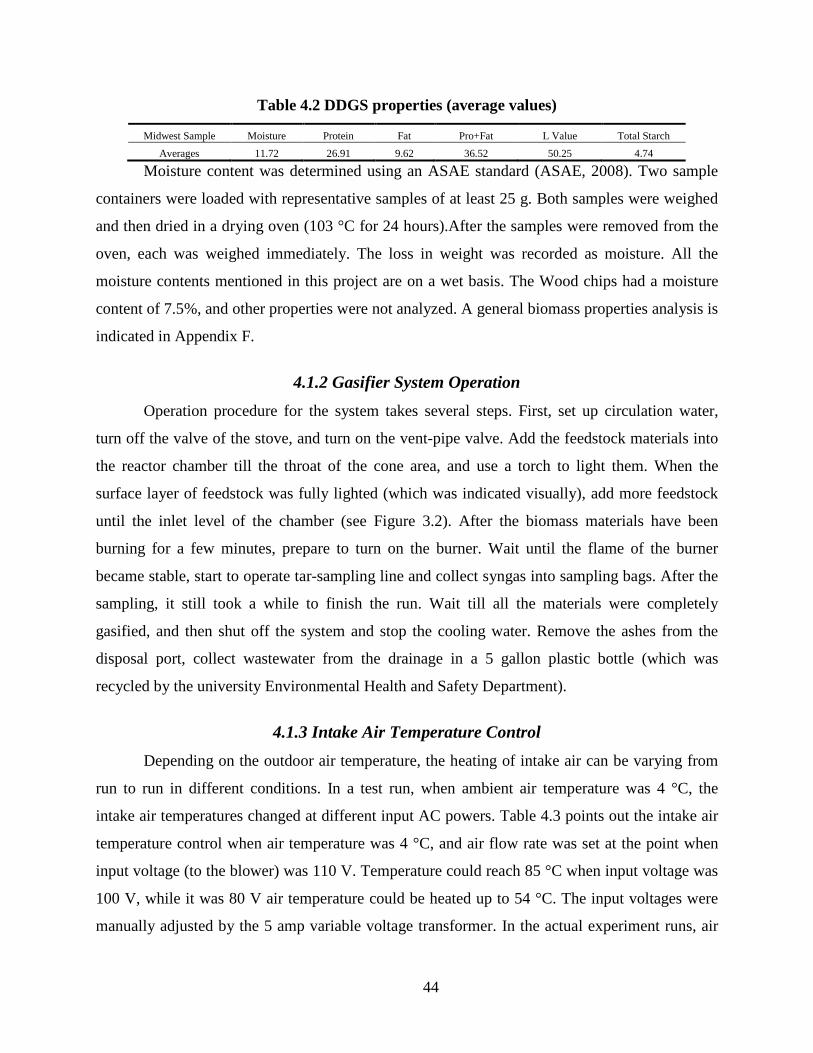
44
Table 4.2 DDGS properties (average values)
Midwest Sample Moisture Protein Fat Pro+Fat L Value Total Starch Averages 11.72 26.91 9.62 36.52 50.25 4.74
Moisture content was determined using an ASAE standard (ASAE, 2008). Two sample
containers were loaded with representative samples of at least 25 g. Both samples were weighed
and then dried in a drying oven (103 °C for 24 hours).After the samples were removed from the
oven, each was weighed immediately. The loss in weight was recorded as moisture. All the
moisture contents mentioned in this project are on a wet basis. The Wood chips had a moisture
content of 7.5%, and other properties were not analyzed. A general biomass properties analysis is
indicated in Appendix F.
4.1.2 Gasifier System Operation Operation procedure for the system takes several steps. First, set up circulation water,
turn off the valve of the stove, and turn on the vent-pipe valve. Add the feedstock materials into
the reactor chamber till the throat of the cone area, and use a torch to light them. When the
surface layer of feedstock was fully lighted (which was indicated visually), add more feedstock
until the inlet level of the chamber (see Figure 3.2). After the biomass materials have been
burning for a few minutes, prepare to turn on the burner. Wait until the flame of the burner
became stable, start to operate tar-sampling line and collect syngas into sampling bags. After the
sampling, it still took a while to finish the run. Wait till all the materials were completely
gasified, and then shut off the system and stop the cooling water. Remove the ashes from the
disposal port, collect wastewater from the drainage in a 5 gallon plastic bottle (which was
recycled by the university Environmental Health and Safety Department).
4.1.3 Intake Air Temperature Control Depending on the outdoor air temperature, the heating of intake air can be varying from
run to run in different conditions. In a test run, when ambient air temperature was 4 °C, the
intake air temperatures changed at different input AC powers. Table 4.3 points out the intake air
temperature control when air temperature was 4 °C, and air flow rate was set at the point when
input voltage (to the blower) was 110 V. Temperature could reach 85 °C when input voltage was
100 V, while it was 80 V air temperature could be heated up to 54 °C. The input voltages were
manually adjusted by the 5 amp variable voltage transformer. In the actual experiment runs, air

45
was introduced without preheating. It was only for the purpose of testing how to manually
control the intake air temperature. Therefore, in the energy efficiency estimates, there was no
extra heat accounted in the final calculation, but only the higher heating value of the biomass.
Table 4.3 Intake air temperature (ambient air temperature = 4 °C)
Voltage (V) Temp (o
80 C)
54 85 60 90 69 95 75 100 85
4.1.4 Tar and Syngas Analysis Syngas sample was collected through the sampling port set in the upper wall of purifier
chamber using a 3 L Tedlar sampling bag (flushed with N2
for at least 3 times and dried in the
oven at 100 °C for 12 hours). Tar samples were collected using the sampling line. Tar samples
are shown in Figure 4.2. In the solution condition, tars were condensed in acetone, which was
indicated by the color of the solution, the darker the color was, the more tars were trapped. After
the tars were dried in the oven, there was a layer of black residue in the bottom of the flask. It is
suggested that both the sample gas and tar should be analyzed immediately after the experiment
run.
Figure 4.2 Tar samples (left, solutions; right, dried)
Analysis was operated in a chemical engineering lab (Dr. Keith Hohn) where a SRI
8610s gas chromatograph (GC) (SRI Instruments, Torrance, CA) equipped with a thermal
conductivity detector (TCD) was set up (Figure 4.3). Helium was used as the carrier gas in the
gas chromatograph (it was required TCD switch could not be turned on until the carrier gas was
supplied). A syringe was used to pump 1 ml of syngas sample from the sampling bag and inject
the sample into the gas chromatograph via the inlet port. For each run, the system needed to

46
warm up to the setpoint temperature (i.e., 29 °C). In order to obtain complete analysis of each
component, it took 20-30 minutes to finish one run. Data analysis of syngas composition was
completed using the SimplePeak software (Figure 4.4). Each peak in the curve indicated a
molecule component, while its peak area was proportional to its amount. Different molecules
exited the GC sampling loop at different times (which was termed as ‘retention time’, with the
unit of second) depending on their molecular weights and some other factors. For the main
syngas components, the typical retention time for each of them was, H2, 1.8s, CO, 7.7-10.6s,
CH4, 5.8-6, CO2, 6.8s. Calibration chart for the GC analysis is shown in Appendix I.
Figure 4.3 Syngas composition analysis using a SRI 8610s GC
Figure 4.4 PeakSimple for GC data analysis
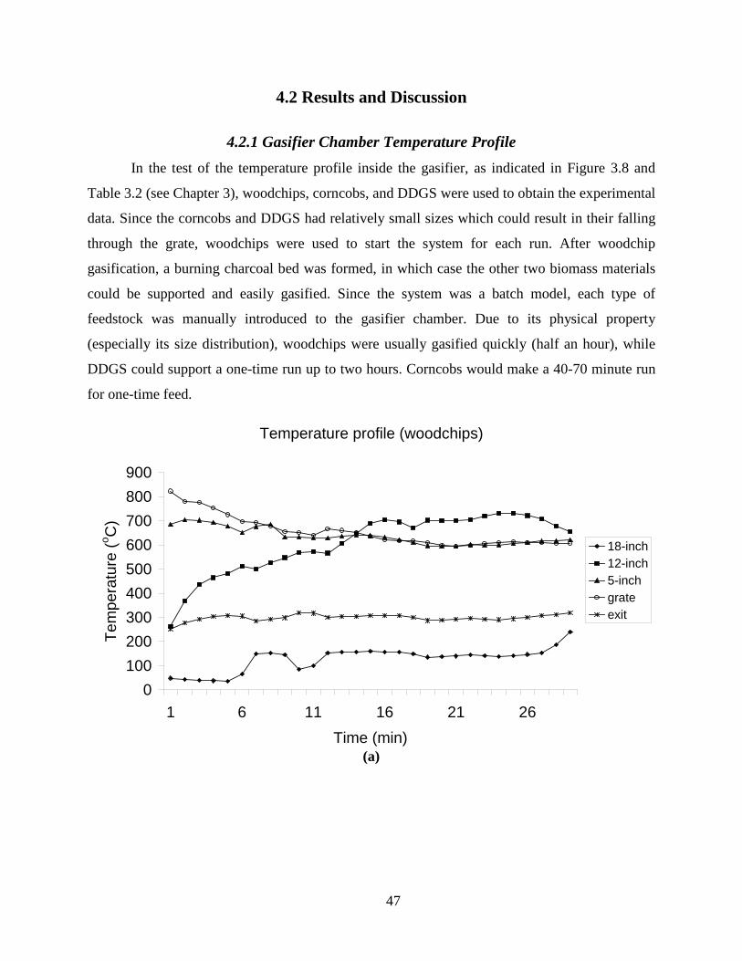
47
4.2 Results and Discussion
4.2.1 Gasifier Chamber Temperature Profile In the test of the temperature profile inside the gasifier, as indicated in Figure 3.8 and
Table 3.2 (see Chapter 3), woodchips, corncobs, and DDGS were used to obtain the experimental
data. Since the corncobs and DDGS had relatively small sizes which could result in their falling
through the grate, woodchips were used to start the system for each run. After woodchip
gasification, a burning charcoal bed was formed, in which case the other two biomass materials
could be supported and easily gasified. Since the system was a batch model, each type of
feedstock was manually introduced to the gasifier chamber. Due to its physical property
(especially its size distribution), woodchips were usually gasified quickly (half an hour), while
DDGS could support a one-time run up to two hours. Corncobs would make a 40-70 minute run
for one-time feed.
Temperature profile (woodchips)
0100200300400500600700800900
1 6 11 16 21 26Time (min)
Tem
pera
ture
(o C)
18-inch12-inch5-inchgrateexit
(a)

48
Temperature profile (woodchips)
0100200300400500600700800900
1 6 11 16 21 26 31Time (min)
Tem
pera
ture
(o C)
18-inch12-inch5-inchgrateexit
Figure 4.5 Temperature profile inside the gasifier for woodchips gasification
As indicated in the temperature profile curves shown in Figure 4.5, within different
reaction zones, temperatures were typically different from each other (in stable stages). This
temperature distribution is very typical for that of a downdraft gasifier. In the starting stage of
gasification, since the gasifier chamber was lighted with a small amount of woodchips,
temperature at the grate was already very high (i.e., 600-800 °C). An occasion for the first figure
(a) was, the temperature at 5-inch was also very high, which was because the woodchips were
burned to the throat (where 5-inch was located) and it was heated up to a high temperature. After
new biomass was feed into the gasifier, temperature at the grate was decreased, while in other
sites temperature increased gradually. In 6-10 minutes, the system approached stable
gasification, and temperatures were relatively stable compared to the starting stage.
Temperatures were 100-200 °C at 18-inch, 700-800 °C at 12-inch, around 600 °C at 5-inch, and
600-700 °C at the grate. Syngas outlet temperature located within a typical range of 280-300 °C.
Both in curves (a) and (b), there was temperature decreasing during the stable stages, like around
the 10-11th min in (a) and the 13-14th
(b)
min in (b), that was because the lid of gasifier chamber was
removed and a metal pole was used to stir the biomass feedstock to prevent biomass bridging and
allow smooth flow of the biomass. However, in this process, cool air poured in, and temperature

49
at 18-inch would decrease. In the shut-off stage, biomass was running out, and reactions were
approaching to the end. During this period, temperatures at the grate, 12-inch and 5-inch tended
to decrease, while temperature at 18-inch and the exit increase (which was because the flame
came close to the upper sites, and the heated air was exiting through the system).
After the starting run of the system, another batch of woodchips was fed into the system.
Since a supporting bed of burning charcoal was formed, the added feedstock could be gasified
very easily and relatively more stable. A typical temperature profile of this process is shown in
Figure 4.5(b). As indicated in this curve, temperature at 18-inch was decreased as new biomass
was added. Oxidation was retrieved when new biomass was reacted and temperature at 12-inch
increased till it approached a steady state. In the stable gasification process, temperature was still
within the ranges as in the starting run. A sharp jump of temperature at 18-inch during the ending
stage was due to the increase of the burning charcoal bed so the flame could reach the upper sites
of the gasifier chamber easily.
Temperature profile (woodchips)
0100200300400500600700800900
1 6 11 16 21 26 31Time (min)
Tem
pera
ture
(o C)
18-inch12-inch5-inchgrateexit
Figure 4.6 Temperature profile of woodchips gasification after the starting run
Corncobs and DDGS were also added into the preheated gasifier system to test their
specific temperature profiles, as shown in Figure 4.7 and Figure 4.8. Corncobs gasification was
similar to that of woodchips, except that its particle size was smaller than that of woodchips.

50
Temperature profiles of both (after the starting run) were quite close to each other. After
corncobs were added, temperature at 18-inch decreased till stable, while temperatures at 12-inch,
5-inch, and grate increased till stable. Temperature at exit was almost kept unchanged. However,
with fine particle sizes, corncobs could support a longer run than the woodchips gasification.
When corncobs were burning out, temperature at 18-inch jumped as expected.
Temperature profile (corncobs)
0
100
200
300
400
500
600
700
800
1 6 11 16 21 26 31 36 41 46 51 56 61 66Time (min)
Tem
pera
ture
(o C)
18-inch12-inch5-inchgrateexit
Figure 4.7 Temperature profile of corncobs gasification after the starting run
Comparatively, woodchips and corncobs could be more easily gasified than DDGS. The
small particle sizes of DDGS made it difficult to handle inside the gasifier. Since DDGS was too
closely packed, air was not easy to go through the DDGS layers to reach in reactions, especially
those most important in the oxidation and reduction zones. Therefore, DDGS was randomly
stirred with the metal pole to prevent bridging and to make some small holes scattering the
DDGS inside the gasifier, enabling air getting in through them. And that was probably why the
temperatures in 18-inch, 12-inch, and 5-inch, were greatly shifting during the gasification
process. In contrast, temperatures in the grate and exit were much more stable. Even though,
since DDGS supported a longer time run, there were several stable stages through the whole
process lasting 20-30 minutes. For instance, from the 110th min to the 130th min, there was a
relatively stable gasification stage. It was noted that temperatures at 12-inch for DDGS
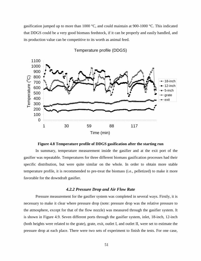
51
gasification jumped up to more than 1000 °C, and could maintain at 900-1000 °C. This indicated
that DDGS could be a very good biomass feedstock, if it can be properly and easily handled, and
its production value can be competitive to its worth as animal feed.
Temperature profile (DDGS)
0100200300400500600700800900
10001100
1 30 59 88 117Time (min)
Tem
pera
ture
(o C)
18-inch12-inch5-inchgrateexit
Figure 4.8 Temperature profile of DDGS gasification after the starting run
In summary, temperature measurement inside the gasifier and at the exit port of the
gasifier was repeatable. Temperatures for three different biomass gasification processes had their
specific distribution, but were quite similar on the whole. In order to obtain more stable
temperature profile, it is recommended to pre-treat the biomass (i.e., pelletized) to make it more
favorable for the downdraft gasifier.
4.2.2 Pressure Drop and Air Flow Rate Pressure measurement for the gasifier system was completed in several ways. Firstly, it is
necessary to make it clear where pressure drop (note: pressure drop was the relative pressure to
the atmosphere, except for that of the flow nozzle) was measured through the gasifier system. It
is shown in Figure 4.9. Seven different ports through the gasifier system, inlet, 18-inch, 12-inch
(both heights were related to the grate), grate, exit, outlet I, and outlet II, were set to estimate the
pressure drop at each place. There were two sets of experiment to finish the tests. For one case,

52
the biomass was not lighted (therefore, no reactions at all), and the other condition was the real
working condition. For the former setting, pressure was measured at each site, while only the
outlet II was tested in the working condition due to high temperatures in the gasifier chamber.
18in
12in
outlet II
outlet I
exit
18in
12in
grate
inlet
Figure 4.9 Pressure drop measurement through the gasifier system
4.2.2.1 Biomass Loading Affecting Pressure Drop
The 5 amp variable voltage transformer was used to control the voltage input to the
blower. Voltages were set to 90 V, 100 V, 110 V, and 120 V. Firstly, without any feed inside the
gasifier chamber, run the system under different power, and record the pressure drop at different
locations. Three different biomass materials were separately fed into the gasifier, and each
resulted in one set of pressure drop data. Each biomass was loaded to the inlet level, so as to
maintain the same height inside the gasifier. The difference in pressure drop with different
biomass material (including no feed) is shown in Figure 4.10.

53
Pressure drop comparison at inlet
No Feed
Wood
Corncobs
DDGS
-1.0
-0.8
-0.6
-0.4
-0.2
0.0
0.2
Biomass
Pre
ssur
e (in
ch o
f wat
er)
Pressure drop comparison at 18-inch
No FeedWood
Corncobs
DDGS
-1.4
-1.2
-1.0
-0.8
-0.6
-0.4
-0.2
0.0
Biomass
Pre
ssur
e (in
ch o
f wat
er)
Pressure drop comparison at 12-inch
No FeedWood
Corncobs
DDGS-1.6-1.4-1.2-1.0-0.8-0.6-0.4-0.20.0
Biomass
Pre
ssur
e (in
ch o
f wat
er)
Pressure drop comparison at grate
No FeedWood
Corncobs DDGS-1.6-1.4-1.2-1.0-0.8-0.6-0.4-0.20.0
Biomass
Pre
ssur
e (in
ch o
f wat
er)
Pressure drop comparison at exit
No FeedWood
Corncobs DDGS-1.6-1.4-1.2-1.0-0.8-0.6-0.4-0.20.0
Biomass
Pre
ssur
e (in
ch o
f wat
er)
Pressure drop comparison at outlet I
No Feed Wood
Corncobs
DDGS0.0
1.0
2.0
3.0
4.0
5.0
6.0
7.0
Biomass
Pre
ssur
e (in
ch o
f wat
er)
Pressure drop comparison at outlet II
No Feed Wood
Corncobs
DDGS
-1.00.01.02.03.04.05.06.07.0
Biomass
Pre
ssur
e (in
ch o
f wat
er)
Figure 4.10 Pressure drop comparison at different locations through the gasifier system
(power input = 120 V)
(a)
(c)
(e) (f)
(d)
(b)
(g)

54
As shown in the curve of inlet pressure drop (a), with DDGS fed, the pressure drop was
almost 0, which was an indicator that DDGS was so closely packed that even the blower could
not bring much pressure change at this location. However, both woodchips and corncobs would
allow small pressure drops, and the pressure drop with corncobs fed was close to the empty
condition (no feed). In the lower sites of the gasfier, each came closer to the blower.
Theoretically, it is easier to form vacuum conditions at the locations close to the blower. That
was proved in the figures (b), (c), (d), and (e), by those negative pressure drops. After the
blower, the pressure drop became positive. As indicated in the figures (b), (c), (d), and (e),
pressure drops were wood<corncobs<DDGS, at the locations ahead of the blower. In contrast,
after the blower, in figures (f) and (g), that was DDGS<corncobs<wood. This was due to the
particle size distribution of each biomass feedstock. Smaller sizes favored stronger negative
pressure drops, and resulted in relatively small positive pressure drop.
4.2.2.2 Voltage Affecting Pressure Drop
For each fixed location, the pressure drop was studied as a function of voltage to the
blower. Its effects are shown in Figure 4.11. As a general rule, pressure drop would increase as
the input voltage was increased, for each type of biomass feedstock and at each location, as
indicated through figures (a) to (g). In curve (a), when DDGS was fed, pressure drop at inlet was
very small and kept constant at 0.1 inch of water. In contrast, negative pressure drops were
created when woodchips and corncobs were fed into the gasifier, and both increased as input
voltages became higher. In figures (d), (e), and (g), pressure drops at the grate, the exit, and
outlet II, were slightly changed as DDGS was fed into the gasifier chamber.
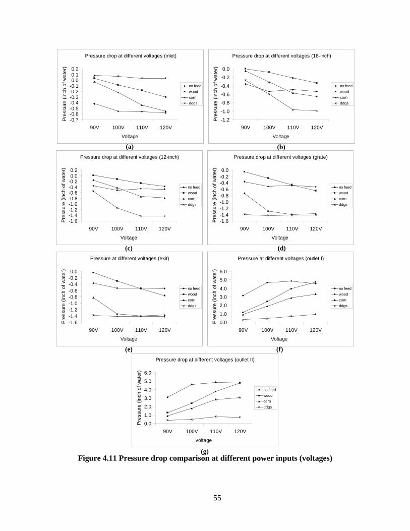
55
Pressure drop at different voltages (inlet)
-0.7-0.6-0.5-0.4-0.3-0.2-0.10.00.10.2
90V 100V 110V 120V
Voltage
Pre
ssur
e (in
ch o
f wat
er)
no feedwoodcornddgs
Pressure drop at different voltages (18-inch)
-1.2
-1.0
-0.8
-0.6
-0.4
-0.2
0.0
90V 100V 110V 120V
Voltage
Pre
ssur
e (in
ch o
f wat
er)
no feedwoodcornddgs
Pressure drop at different voltages (12-inch)
-1.6-1.4-1.2-1.0-0.8-0.6-0.4-0.20.00.2
90V 100V 110V 120V
Voltage
Pre
ssur
e (in
ch o
f wat
er)
no feedwoodcornddgs
Pressure drop at different voltages (grate)
-1.6-1.4-1.2-1.0-0.8-0.6-0.4-0.20.0
90V 100V 110V 120V
Voltage
Pre
ssur
e (in
ch o
f wat
er)
no feedwoodcornddgs
Pressure at different voltages (exit)
-1.6-1.4-1.2-1.0-0.8-0.6-0.4-0.20.0
90V 100V 110V 120V
Voltage
Pre
ssur
e (in
ch o
f wat
er)
no feedwoodcornddgs
Pressure at different voltages (outlet I)
0.0
1.0
2.0
3.0
4.0
5.0
6.0
90V 100V 110V 120V
Voltage
Pre
ssur
e (in
ch o
f wat
er)
no feedwoodcornddgs
Pressure drop at different voltages (outlet II)
0.0
1.0
2.0
3.0
4.0
5.0
6.0
90V 100V 110V 120V
voltage
Pre
ssur
e (in
ch o
f wat
er)
no feedwoodcornddgs
Figure 4.11 Pressure drop comparison at different power inputs (voltages)
(a)
(c) (d)
(b)
(e) (f)
(g)

56
Generally, pressure drops at the locations ahead of the blower were smaller than 1.6
inches of water, while pressure drops were within 5 inches of water, after the blower.
4.2.2.3 Pressure Drop Variations at Different Locations
Pressure drop was studied as a function of location, under a specific power input. It is
shown in Figure 4.12. All four graphs were in the same shapes that indicated similar variations
under different voltages. Compared to no feed, when woodchips were fed, pressure drop became
less significant as voltages were increased. For each curve, the pressure drop difference was 2
inches of water at 90 V (a); 2 inches of water at 100 V (b); 1 inch of water at 110 V (c); and
almost 0 at 120 V (d). Difference between pressure drop when corncobs were fed and when
DDGS was fed became more significant as voltages increased. For each curve, the pressure drop
difference was less than 1 inch of water at 90 V (a); more than 1 inch of water at 100 V (b); more
than 2 inches of water at 110 V (c); and more than 2 inches of water at 120 V (d).
Also indicated from curves (a) through (d) in Figure 4.12, ahead of the blower, pressure
drop approached maximum at exit which was closest to the blower. After the blower, pressure
drop decreased after the filtrator, but not that big change in values. Compared to pressure drops
after the blower, pressure drops at the locations ahead of the blower were quite close in values.

57
Pressure drop at 90V
-2.0
-1.0
0.0
1.0
2.0
3.0
4.0
inlet 18in
12in
grate ex
it
outle
t I
outle
t II
Location
Pre
ssur
e (in
ch o
f wat
er)
No Feed
Woodchips
Corncobs
DDGS
Pressure drop at 100V
-2.0
-1.0
0.0
1.0
2.0
3.0
4.0
5.0
6.0
inlet 18in
12in
grate ex
it
outle
t I
outle
t II
Location
Pre
ssur
e (in
ch o
f wat
er)
No Feed
Woodchips
Corncobs
DDGS
(a)
(b)

58
Pressure drop at 110V
-2.0
-1.0
0.0
1.0
2.0
3.0
4.0
5.0
6.0
inlet 18in
12in
grate ex
it
outle
t I
outle
t II
Location
Pre
ssur
e (in
ch o
f wat
er)
No Feed
Woodchips
Corncobs
DDGS
Pressure drop at 120V
-2.0
-1.0
0.0
1.0
2.0
3.0
4.0
5.0
6.0
inlet 18in
12in
grate ex
it
outle
t I
outle
t II
Location
Pre
ssur
e (in
ch o
f wat
er)
No Feed
Woodchips
Corncobs
DDGS
Figure 4.12 Pressure drop at different locations across the gasifier system
(c)
(d)

59
4.2.2.4 Pressure Drop at Outlet II
During each run of the gasification of three different biomass feedstocks, the pressure
drop at outlet II was also recorded. This measurement gave information of pressure drop
variation during the gasification process at that specific location. Results are shown in Figures
4.13, 4.14, and 4.15 (note: err bars are from the standard deviation which is shown in Appendix
C). Through the gasification process, pressure drop at outlet II decreased slightly for each type of
biomass feedstock. Pressure drops were in the ranges of 3-5 inches of water for woodchips
gasification, 2-4 inches of water for corncobs gasification, and 1-2.5 inches of water for DDGS
gasification. The variation of pressure drops was more significant for DDGS gasification than
that for corncobs gasification. The variation was not that significant for woodchips gasification,
compared to both DDGS and corncobs.
Pressure drop at outlet II (woodchips)
0.0
1.0
2.0
3.0
4.0
5.0
6.0
7.0
8.0
0 5 10 15 20 25 30 35 40Time (min)
Pre
ssur
e (in
ch o
f wat
er)
Figure 4.13 Pressure drop at outlet II for woodchips gasification

60
Pressure drop at outlet II (corncobs)
0.0
1.0
2.0
3.0
4.0
5.0
6.0
7.0
0 10 20 30 40 50 60 70Time (min)
Pre
ssur
e (in
ch o
f wat
er)
Figure 4.14 Pressure drop at outlet II for corncobs gasification
Pressure drop at outlet II (DDGS)
0.0
0.5
1.0
1.5
2.0
2.5
3.0
3.5
4.0
0 29 58 87 116 145Time (min)
Pre
ssur
e (in
ch o
f wat
er)
Figure 4.15 Pressure drop at outlet II for DDGS gasification

61
4.2.2.5 Pressure Drop of the Flow Nozzle and Syngas Flow Rate
Pressure drop across the flow nozzle, which was set in the syngas outlet after the
purification system, was estimated to determine the syngas yield rate. It was also an indicator of
the stability of the gasifier system. And, when proportionally changed the power input for the
DC motor, we could accordingly change the value of intake air flow rate and the syngas yield
rate could be varied with a certain pattern. Calculations of the syngas flow rate could be
completed under the specific exiting syngas conditions. Table 4.4 indicates the pressure drop
across the flow nozzle under different input voltage for the DC motor.
Table 4.4 Pressure drop across the flow nozzle and syngas flow rate Voltage (V) ∆P (Pa) Syngas flow rate (cfm)
90 32.4 9.3 100 69.7 13.7 110 122.0 18.1 120 159.4 20.7
4.2.3 Syngas Composition Compositions (v%) of the syngas are shown in Table 4.5.
Table 4.5 Syngas composition Molecule Wood Chips DDGS
H 20.04% 2 19.08%
O 3.15% 2 1.18%
N 61.64% 2 50.70%
CO 0.04% 2 7.65%
CO 15.01% 20.02%
CH 0.12% 4 1.34%
For syngas generated from atmospheric, air blown downdraft gasifiers, H2
4.2.4 Tar Concentration
usually ranges
from 15-21%, and CO 10-22% (Heesch et al., 1999). Our results were consistent with reported
values.
The gas sampling rates were 9.3 L/min and 9.8 L/min for wood chips and DDGS,
respectively. The total sampling volume and tar concentration are listed in Table 4.6. For
downdraft gasifiers, the general range of tar concentration is 0.5-5 g/Nm3 (Milne et al., 1998),
depending on gasifier designs and biomass feedstocks. Our results were located in this range.

62
Table 4.6 Tar concentration Biomass Sampling volume Tar concentration
Wood Chips 140.2 L 1.65 g/NmDDGS
3 147.3 L 4.20 g/Nm
4.2.5 Gasification Energy Efficiency
3
Comparison of biomass energy content with syngas energy value resulted in the
gasification efficiency.
( ) ( )woodchipsbiowoodchips HHVMCWE ×−×= 1
( )syngasvsyngas HHVqtE ××=
%100×=syngas
woodchips
EE
η
70.2%)(4574.0 −×= CHHVwoodchips
%)(781.39%)(622.12%)(769.12 42 CHCOHHHVsyngas ×+×+×=
Where,
Ewoodchips
E
, the energy content of woodchips (MJ)
syngas
W
, the energy content of syngas (MJ)
woodchips,
MC, the moisture content of woodchips (%)
the mass of woodchips (kg)
t, the duration of stable gasification (minute)
qv
η, the gasification efficiency (%)
, volume flow rate of syngas (cfm)
HHVwoodchips
HHV
, HHV of woodchips (MJ/kg)
syngas, HHV of syngas (MJ/m3
C%, the carbon content in woodchips (dry basis)
)
H2%, CO%, and CH4
Calculation of HHV of woodchips was based on the following formula (Brown, 2003).
%, the percentage of syngas components
2.70- biomass)dry on (C%0.4574 kgMJ/dry in HHV ×=
The resulted HHV for woodchips was 17.54 MJ/kg (dry basis).
Based on the thermodynamic data used by National Renewable Energy Laboratory (IEA,
2001) (see Appendix J), the following calorific values were used to compute the HHV (unit:
MJ/m3 at standard conditions) of syngas (Table 4.7).

63
Table 4.7 Calorific values (MJ/Nm3
Component
) for syngas components (IEA, 2001)
H CO 2 CH C4 2H C6 2H C4 2HHHV
2 12.769 12.622 39.781 69.693 63 58.059
LHV 10.788 12.622 35.814 63.748 59.036 56.078
Based on the syngas composition of woodchips gasification and their calorific values, the
syngas HHV was calculated, which was 4.50 MJ/m3. It was assumed that syngas heating value
was constant in this calculation, regardless of the wood moisture contents. Therefore in the
calculation of energy efficiency, for woodchips gasification, syngas heating value was 4.50
MJ/m3
Eight runs of woodchips gasification were tested, of which the energy efficiencies were
estimated (Figure 4.16). It was noted that energy efficiency at the starting run was relatively
lower compared to the runs after the burning charcoal was formed. Energy efficiency for wood
chips gasification was 36.0% ± 7.7%.
, higher heating value for wood chips was 17.54 MJ/kg. Calculation was completed in an
Excel spreadsheet in Table 6.11 (Appendix I).
Energy efficiency for woodchips gasification
0%10%20%30%40%50%60%70%80%90%
100%
1 2 3 4 5 6 7 8
η (%
)
Run
Figure 4.16 Energy efficiency for woodchips gasification

64
4.3 Summary Three different types of biomass feedstock, woodchips, corncobs, and DDGS, were used
to conduct the experimental study. Woodchips were used to initiate the starting run, and after
that a burning charcoal was formed to support new feedstock added into the gasifier chamber. As
indicated in the temperature profile curves, temperature values were typically different from each
other in different reaction zones.
Intake air temperature was manually controlled by the high-flow-rate heater together with
the variable voltage transformer. However, in the experiment runs of the three biomass
feedstock, air was not preheated.
Pressure drop and air flow rate were measured and calculated. During the non-working
condition, three biomass materials were loaded in the gasifier, data was collected to compare the
pressure drops at different locations through the gasifier system, also under the power inputs set
at four different levels. Negative pressure drop tended to increase when it came close to the
blower, while positive pressure drop after the blower was decreased after the filtrator.
The test showed that the syngas composition, carbon monoxide (15%-20%v) and
hydrogen (19%-20%v), and tar concentration, 1.65-4.20 g/Nm3 were typical for a downdraft
gasifier. Energy efficiency for wood chips gasification was 36.0% on average.

65
CHAPTER 5 - Summary
A downdraft gasifier system was instrumented and tested. Three instrumentation
components were designed and built into the gasifier system: real-time temperature monitoring,
differential pressure measurement, and gas flow rate measurement. Moreover, a full-wave
rectifier circuit was applied to convert the AC power to DC power plus the regulation of AC
input via a variable voltage transformer. A high-flow-rate heater was also setup to control intake
air temperature. A tar sampling method based on the IEA tar protocol was developed.
Experimental studies using three different biomass materials were performed to test the design
and construction of these two systems.
Major achievements of this research are:
• Chromel-Alumel type-K thermocouples with a signal-conditioning device were chosen
and installed to monitor the temperatures inside the gasifier. A differential pressure
transducer and an ISA1932 flow nozzle were installed to measure pressure drop and gas
flow rate of the system, respectively. Measured temperature profile inside the gasifier
was comparable to that of a typical downdraft gasifier. Measured gas flow rate was close
to the gasifier specification.
• A modified IEA tar protocol was used to determine tar concentration in syngas. Acetone
was used as the condensation solvent to trap tars in the syngas. Wood chips and DDGS
were tested as the feedstocks for biomass gasification experiments. The test showed that
the syngas composition, carbon monoxide (15%-20%v) and hydrogen (19%-20%v), and
tar concentration, 1.65-4.20 g/Nm3 were typical for a downdraft gasifier. Energy
efficiency for wood chips gasification was 36.0% on average.

66
CHAPTER 6 - Future Research Recommendations
The purpose of this research was focused on instrumentation and tar measurement of a
downdraft gasifier. Based on research work completed, this project can be further developed in
all following studies.
• Change the intake air temperature, biomass moisture content, and air flow rate to test how
operating parameters would affect gasification performance.
• Test more types of biomass feedstock to study the capability of the downdraft gasifier
system and compare the performance for each biomass.
• Verify the tar measurement system by comparing with some other methods.
• Add steam injection and provide better insulation (to reduce heat loss), so as to improve
the existing system.
67
References
Abatzoglou, N.; Fernandez, J.-C.; Laramee, L.; Jollez, P.; Chornet, E. 1997a. “Application of Gasification to the
Conversion of Wood, Urban and Industrial Wastes,” in Developments in Thermochemical Biomass Conversion,
Vol. 2. Edited by A.V. Bridgwater and D.G.B. Boocock. London: Blackie Academic & Professional, pp. 960–
972.
Adegoroye, A., N. Paterson, X. Li, T. Morgan, A.A. Herod, D.R. Dugwell, and R. Kandiyoti. 2004. The
characterisation of tars produced during the gasification of sewage sludge in a spouted bed reactor. Fuel (83):
1949-1960.
ASAE Standards, 2008. S358.2 DEC 1988 (R2008). Moisture measurement – forages. St. Joseph, MI: American
Society of Agricultural Engineers.
ASME Standards. 2004. MFC-3M-2004: Measurement of fluid flow in pipes using orifice, nozzle, and venture. New
York, N.Y.: ASME.
Baker, E.G., R.H. Moore, L.K. Mudge, and D.C. Elliott. 1986. “Engineering Analysis of Biomass Gasifier Product
Gas Cleaning Technology,” Richland, WA: Battelle Memorial Institute, Biofuels and Municipal Waste
Technology Division, PNL-5534.
Baker, E.G.; M.D. Brown, D.C. Elliott, and L.K. Mudge.1988. “Characterization and Treatment of Tars from
Biomass Gasifiers,” Denver, CO: AIChE 1988 Summer National Meeting. 1–11.
Bangala, D. 1997. “Reformage Catalytique de Naphtalene et Ai-chlos-benzene,” Ph.D. Thesis, Universite de
Sherbrooke, Faculte des Sciences Appliques, Department de Genie Chimque.
Biomass Technology Group (BTG). 1995b. “Development of a Standard Procedure for Gas Quality Testing in
Biomass Gasifier Plant/Power Generation Systems.” Final report. The Netherlands: BTG Biomass Technology
Group, JOU2-CT93-0408, NOVEM. EWAB-9608.
Biomass Technology Group (BTG). 2008. Tar & Tar Measurement. Available at:
http://www.btgworld.com/index.php?id=21&rid=8&r=rd. Accessed 16 December 2008.
Blades, T., M. Rudloff, and O. Schulze. 2005. Sustainable SunFuel from CHOREN’s Carbo-V® Process. CHOREN
Industries Freiberg, Presented at ISAF XV, San Diego

68
Blanco, C.G., J. Blanco, P. Bernad, and M.D. Guillen. 1991. J. Chromatogr.(539): 157
Blanco, C.G., J.S. Canga, A. Dominguez, M.J. Iglesias, and M.D. Guillen. 1992. J. Chromatogr. (607): 295
Bodalo, A., G. Leon, M.L. Asanza, and E. Gomez. 1994. J.H. Resolut. Chromatogr. (17): 20
Bombach, R. 2002. Application of Raman spectroscopy: Species concentration and temperature measurements for
catalytically stabilized combustion. ERCOFTAC SUMMER SCHOOL, March 2002, Zurich.
Brage, C., and K. Sjostrom. 1991. Separation of phenols and aromatic hydrocarbons from biomass tar using
aminopropylsilane normal-phase liquid chromatography. J. Chromatogr. A (538): 303-310
Brage, C., Q. Yu. and K. Sjöström. 1996. Characteristics of evolution of tar from wood pyrolysis in a fixed-bed
reactor. Fuel (75): 213-219.
Brown, M.D., E.G. Baker, and L.K. Mudge. 1986. Evaluation of processes for removal of particulates, tars, and oils
from biomass gasifier product gases. In: Proc. Energy from Biomass & Waste X. London-New York: Elsevier
Sci. 655-676.
Brown, R. 2003. Biorenewable resources: engineering new products from agriculture. Wiley-Blackwell: NJ
Brussels. 1988. IEA Thermal Gasification of Biomass Task, EC and USDOE Meeting on Tar Measurement
Protocol. March 18–19, Brussels, Belgium. Meeting Presentation Information.
Carpenter, D.L., S.P. Deutch, and R.J. French. 2007. Quantitative measurement of biomass gasifier tars using a
molecular-beam mass spectrometer: comparison with traditional impinger sampling. Energy & Fuel 21(5): 3036-
3043.
Corella, J., M.P. Aznar, J. Delagado, and E. Aldea. 1991. Steam gasification of cellulosic wastes in a fluidized bed
with downstream vessels. Ind. Eng. Chem. Res. (30): 2252-2262.
CRE Group Ltd. 1997. “Identification and Processing of Biomass Gasification Tars,” Energy Technology Support
Unit (ETSU), Department of Trade and Industry, DTI Contract No. B/T1/00418/00/00.
Dayton, D.C., R.J. French, and T.A. Milne. 1995. Direct Observation of Alkali Vapor Release during Biomass
Combustion and Gasification. 1. Application of Molecular Beam/Mass Spectrometry to Switchgrass Combustion.
Energy Fuels, 9 (5): 855-865.
Desilets, D.J., P.T. Kissinger, F.E. Lytle, M.A. Horne, M.S. Ludwicszak, and R.B. Jacko. 1984. Determination of
polycyclic aromatic hydrocarbons in biomass gasifier effluents with liquid chromatography/diode array
spectroscopy. Envron. Sci. Technol. (18): 386-391.

69
Donnot, A., J. Reningovolo, P. Magne, and X. Deglise. 1985. Flash pyrolysis of tar from the pyrolysis of pine bark.
J. Anal.Appl.Pyrolysis. (8): 401
Dufour A, P. Girods, E. Masson, S. Normand, Y. Rogaume, and A. Zoulalian. Comparison of two methods of
measuring wood pyrolysis tar. J Chromatogr A. (1164):240-247.
Elliott, D.C. 1988. Relation of reaction time and temperature to chemical composition of pyrolysis oils. In: Soltes
J,Milne TA, editors. Pyrolysis oils from biomass; producing, analysing and upgrading, ACS Symposium Series
376. Washington, DC: American Chemical Society. 55–78.
EPA. 1983. EPA Federal Register 36, No. 247, 24878. Method 5. Determination of particulate emissions from
stationary sources. In: 40 Code of Federal Regulations, Part 60, App. A-Reference methods. Revised 1 July 1983.
Washington: EPA. 437-452.
Evans, R.J. and T.A. Milne. 1987. Molecular characterization of the pyrolysis of biomass. Energy & Fuels.
1(2):123–137
Evans, R.J., and T.A. Milne. 1987. Molecular characterization of the pyrolysis of biomass. 2. Applications. Energy
Fuels 1 (4):311-319
FAO. 1986. Document: Wood gas as engine fuel. Forest Industries Division, Food and Agriculture Organization,
United Nations, 00100 Rome, Italy.
Gaur, S. and T. Reed. 1998. Thermal data for natural and synthetic fuels, Marcel Dekker, New York.
Graboski, M. and R.L. Bain. 1979. "Properties of Biomass Relevant to Gasification," Chapter 3 of A Survey of
Biomass Gasification - Volume 2, Solar Energy Research Institute, SERI/TR-33-239, National Renewable
Energy Laboratory, Golden, CO.
Haser, P., and T. Nussbaumer. 1998. Guideline for sampling and analysis of tars and particulates from biomass
gasifiers. Swiss Federal Office of Energy, Berne.
Hasler, P.; Bühler, R.; Nussbaumer, T. 1997. “Evaluation of Gas Cleaning Technologies for Small Scale Biomass
Gasifiers.” Zurich: Swiss Federal Office of Energy and Swiss Federal Office for Education and Science.
Heesch, E.J.M., A.J. Pemen, M. Keping, S.V.B Yan, S.V.B. Paasen, and K.J. Ptasinski. 1999. Experimental program
of the pulsed corona tar cracker. In: Proc. 12th IEEE Int Pulsed Power Conf. IEEE, New York.
Herzberg, G. 1967. Molecular spectra and molecular structure, I. Spectra of diatomic molecules. 2nd ed. Princeton,
NJ: Twelfth printing; 1967.

70
International Energy Agency (IEA). 2001. Heating value of gases from biomass gasification. Report prepared for
IEA Bioenergy Agreement, Task 20 – Thermal Gasification of Biomass. Report no. TPS-01/16.
Karellas, S., and J. Karl. 2007. Analysis of product gas from biomass gasification by means of laser spectroscopy.
Optics and Lasers in Engineering (45): 935-946.
Kinoshita, C.M., Y. Wang, and J. Zhou. 1994. Tar formation under different biomass gasification conditions.
Journal of analystical ans applied pyrolysis (29):169-181.
Knoef, H.A.M. 2000. The UNDP/World Bank monitoring program on small scale biomass gasifiers (BTG’s
experience on tar measurement). Biomass and Bioenergy (18): 39-54.
Knoef, H.A.M. 2005. Handbook Biomass Gasification. Netherlands: BTG Biomass Technology Group.
Li, X.T., J.R. Grace, C.J. Lim, A.P. Watkinson, H.P. Chen, and J.R. Kim. 2004. Biomass gasification in a circulating
fluidized bed. Biomass and Bioenergy (26): 171-193.
Long, D.A. 1977. Raman spectroscopy. New York, NY: McGraw-Hill.
McKendry, P. 2002. Energy production from biomass (part 3): gasification technologies. Bioresource Technology.
83: 55-63
Milne, T.A., R.J. Evans, and N.Abatzoglou. 1998. Biomass gasification “tars”: their nature, formation and
conversion. NREL, Golden, CO. Report no. NREL/TP-570-25357.
Moersch, O.; Spliethoff, H.; Hein, K.R.G. 1997. “A New System for Tar Sampling and Analysis,” in Biomass
Gasification and Pyrolysis. Edited by M. Kaltschmitt and A.V. Bridgwater. Newbury, UK: CPL Press, pp. 228–
234.
Moersch, O.; H. Spliethoff, and K.R.G. Hein. 1998. “Quasi continuous tar quantification with a new online
analyzing method”, 10th European Conference and technology exhibition, Biomass for Energy and Industry,
Wurzburg, Germany, 8-11 June 1998, Proceedings of the international conference. 1638-1641.
Moersch, O., H. Spliethoff, and K.R.G. Hein. 2000. Tar quantification with a new online analyzing method. Biomass
and Bioenergy (18): 79-86
Nieminen, M.; Simell, P.; Leppälahti, J.; Ståhlberg, P.; Kurkela, E. 1996. “High-Temperature Cleaning of Biomass
Derived Fuel Gas,” in Biomass for Energy and Environment: Proceedings of the 9th European Bioenergy
Conference, June 1996. Edited by P. Chartier et al. Pergamon, pp. 1080–1085.

71
Osipovs, S. 2008. Sampling of benzene in tar matrices from biomass gasification using two different solid-phase
sorbents. Anal Bioanal Chem (391):1409-1417.
Pakdel, H., and C. Roy. 1991. Hydrocarbon content of liquid products and tar from pyrolysis and gasification of
wood. Energy & Fuels (5):427–436
Podgórska, A., K. Sylwester, B. Wlodzimierz. 2006. Effect of operating conditions on tar and gas composition in
high temperature air/steam gasification (HTAG) of plastic containing waste. Fuel Process Technol (87): 223–33.
Qin, Y., H. Huang, Z. Wu, J. Feng, W. Li, and K. Xie. 2007. Characterization of tar from sawdust gasified in the
pressurized fluidized bed. Biomass and Bioenergy (31): 243-249.
Quaak, P., H. Knoef, and H.E. Stassen. 1999. Energy from biomass: a review of combustion and gasification. World
Bank Technical Paper No. 422
Sousa, L.C.R..2001. Gasification of wood, urban waste wood (Altholz) and other wastes in a fluidised bed reactor.
Ph.D. thesis. Swiss Federal Institute of Technology Zurich.
Sricharoenchaikul, V., W.J. Frederick, Jr., and P. Agrawal. 2002. Black Liquor Gasification Characteristics. 2.
Measurement of Condensable Organic Matter (Tar) at Rapid Heating Conditions. Ind. Eng. Chem. Res. (41):
5650–5658
Stassen, H. E. M. and H. A. M. Knoef. 1993. Small-scale gasification systems. The Netherlands: Biomass
Technology Group, University of Twente.
Stobbe, S. J. Oatley, and R.C. Brown. 1996. Indirectly heated biomass gasification using Latent-heat Ballasting of a
Fluidized reactor. In proceedings of the 31st Intersociety. Energy conversion engineering conference, 1996.
IECEC 96.
Turare, C. 2002. Biomass Gasification – Technology and Utilization. Humanity Development Library: Document
text. ARTES Institute, Glucksburg (Germany)
Walawender, W.P., S.M. Chern, and L.T. Fan. 1985. Wood chip gasification in a commercial downdraft gasifier. In:
Overend, R.P., Milne, T.A. & Mudge, L.K. (eds.) Fundamentals of thermochemical biomass conversion. London:
Elsevier. 911-921.
Walsh, M. E., R. L. Perlack, A. TUrhollow, D. G. de la Torre Ugarte, D. A. Becker, R. L. Graham, S. E. Slinshy,
and D. E. Ray. 2000. Biomass feedstock availability in the United States: 1999 state level analysis. Oak Ridge,
TN: Oak Ridge National Laboratory, April 1999, updated January 2000

72
Xu, M., R.C. Brown, G. Norton, and J. Smeenk. 2005. Comparison of a solvent-free tar quantification method to the
International Energy Agency’s tar measurement protocol. Energy & Fuels (19): 2509-2513.

73
Appendix A - Operating Manual for Downdraft Biomass Gasifier
1. Gasifier run: (1) Circulation water set up. (2) Through the left water inlet, add water in to the chamber underneath the filter case till
12-14 cm (controlled by an overflow outlet). (3) Turn off the valve of the stove, turn on the vent-pipe valve. (4) Connect the variable transformer to the wall power. Power on. (5) Add 50 vol % of the wood chips into the reactor chamber, add a small amount of
ethanol to the upper cover of the chips, together with 5-6 pieces of charcoal, use torch to light them so as to start the gasification process (record this initial time
(6) When the wood chips are fully lighted, add more wood chips until the chamber is 90% volume full.
).
(7) After the chips have been burning for a few minutes (record the time
(8) Turn on the pulse switch on the stove first, and then let the switch (which controls the gas from the purifier to the stove) on.
), prepare to turn on the stove.
(9) Wait until the flame of the stove becomes stable (treat it as a signal of stable gasification status, record time
(10) Start to operate Tar/Particulate sampling line (
), using the sampling port after the purifier to collect syngas sample (~80% of the 3 L sampling bag, ~2.4 L).
record time). Make the sample for about 10~15 minutes (record time
2. Syngas sample collection: ). Also read sampling flow rate every 3 minutes.
(1) Connect the filter holder (with 2 pieces of glass fiber filter set up) to the post-purifier sampling port
(2) Connect the outlet of the filter holder to the inlet of sampling bag (3) Collect around 2.4 L syngas sample (80% capacity of the bag)
3. Tar/Particulate sampling: (1) Airproof/airtight test. (2) Connect the tube to the sampling point, set up the filter holder, connect the flow
meter to tube extended from the last sampling bottle, turn on the vacuum pump. Put the
(3) Record the initial time of the sampling. Operate the sampling test for 15~30 minutes. Record the time when we stop sampling.
sampling bottles #1, 2, 4 in the warm water bath; #3, 5, 6 in the ice bath.
(4) Collect the filter paper and other stuffs (stainless pipes and hoses) for analysis. 4. Tar/Particulate analysis:
(1) Wash the sampling line along the syngas flow direction, collect the acetone mixture in one of the sampling bottles.
(2) Use the thimble filter to collect the PM contained in the acetone mixture. (3) Turn on the heater. Set the heater temperature to 80 °C (acetone boiling point =56.53
°C). (4) Set up the Soxhlet apparatus in the lab.

74
(5) Carefully fill the filter paper (with tars and particulates) into the thimble, which is loaded into the main chamber of the Soxhlet extractor.
(6) Place the Soxhlet extractor onto a flask containing the solvent (acetone, 100 ml). (7) Connect the cooling water in port to the tap, and the cooling water out port to the
sink. Equip the extractor to the condenser. (8) As the temperature gradually increases, the main chamber slowly fills with the warm
solvent. The tars contained in the particulate filter paper will be partly solved in acetone. Before the solvent fills the chamber “full” (till the siphon point), remove the acetone to the recycled bottle.
(9) Use recycled acetone to wash each sampling bottle for one time. (10) Remove the thimble from the Soxhlet chamber, dry them (thimble + filter paper)
in the oven (105 °C, 2 hours). (11) Solvent evaporation. (12) Weigh dried “thimble + filter paper” (particulates) and “residues” (tars), use mass
gravimetric method to evaluate weight of particulates.
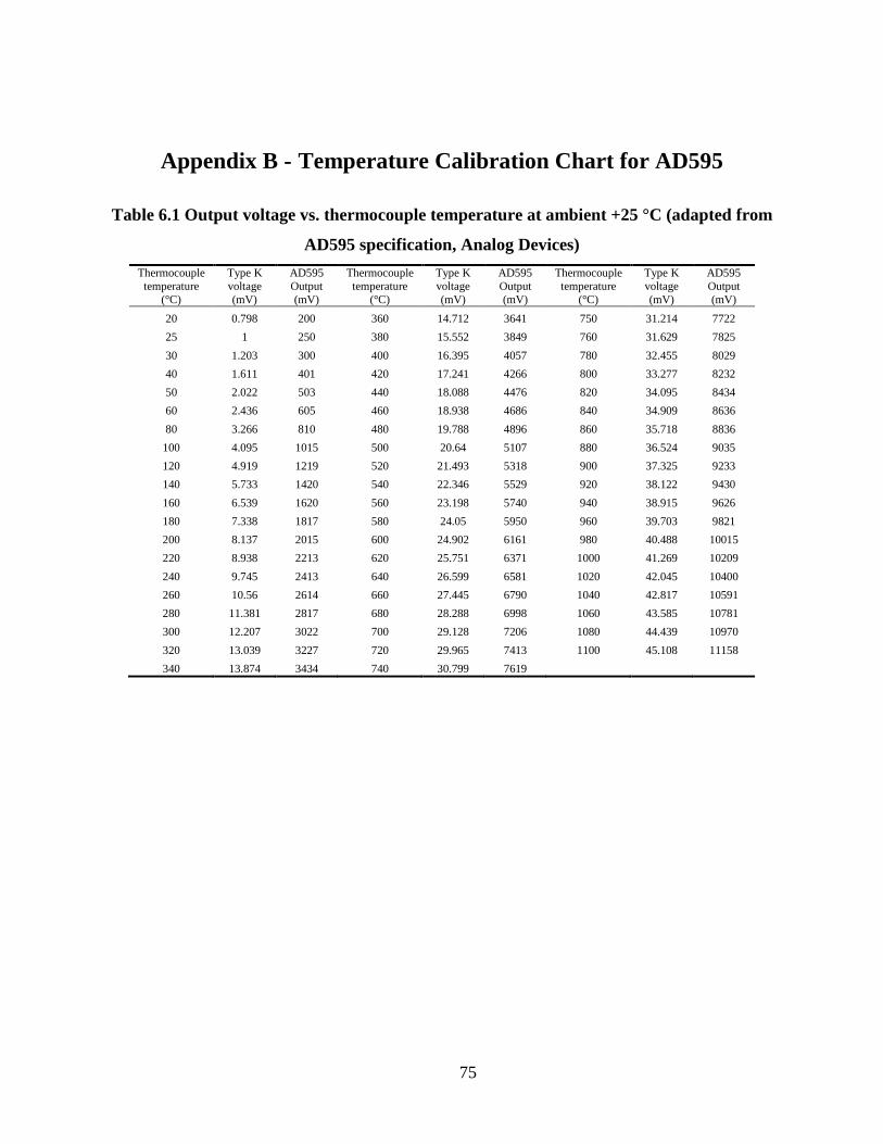
75
Appendix B - Temperature Calibration Chart for AD595
Table 6.1 Output voltage vs. thermocouple temperature at ambient +25 °C (adapted from
AD595 specification, Analog Devices) Thermocouple
temperature (°C)
Type K voltage (mV)
AD595 Output (mV)
Thermocouple temperature
(°C)
Type K voltage (mV)
AD595 Output (mV)
Thermocouple temperature
(°C)
Type K voltage (mV)
AD595 Output (mV)
20 0.798 200 360 14.712 3641 750 31.214 7722 25 1 250 380 15.552 3849 760 31.629 7825 30 1.203 300 400 16.395 4057 780 32.455 8029 40 1.611 401 420 17.241 4266 800 33.277 8232 50 2.022 503 440 18.088 4476 820 34.095 8434 60 2.436 605 460 18.938 4686 840 34.909 8636 80 3.266 810 480 19.788 4896 860 35.718 8836
100 4.095 1015 500 20.64 5107 880 36.524 9035 120 4.919 1219 520 21.493 5318 900 37.325 9233 140 5.733 1420 540 22.346 5529 920 38.122 9430 160 6.539 1620 560 23.198 5740 940 38.915 9626 180 7.338 1817 580 24.05 5950 960 39.703 9821 200 8.137 2015 600 24.902 6161 980 40.488 10015 220 8.938 2213 620 25.751 6371 1000 41.269 10209 240 9.745 2413 640 26.599 6581 1020 42.045 10400 260 10.56 2614 660 27.445 6790 1040 42.817 10591 280 11.381 2817 680 28.288 6998 1060 43.585 10781 300 12.207 3022 700 29.128 7206 1080 44.439 10970 320 13.039 3227 720 29.965 7413 1100 45.108 11158 340 13.874 3434 740 30.799 7619

76
Appendix C - Data of Temperature Profiles and Pressure Drop
Table 6.2 DDGS gasification
Temperature (°C) ∆P (outlet II) (inch of water) 18-inch 12-inch 5-inch grate exit average stdev
153 193 418 522 195 2.4 0.9 144 191 440 556 197 2.0 1.0 140 222 459 587 200 2.3 1.1 143 278 471 615 210 2.1 1.1 142 340 491 643 215 2.1 0.9 131 404 522 662 210 2.1 0.8 110 486 574 667 192 2.0 0.9 129 559 554 669 216 2.2 0.9 133 597 562 670 224 2.2 1.0 140 618 564 675 233 1.9 1.0 142 637 567 681 238 1.9 0.8 145 652 567 690 243 2.0 1.0 146 685 574 697 246 2.0 0.8 117 702 640 688 218 1.9 0.8 117 698 659 684 219 1.7 0.8 118 702 669 681 221 2.0 0.8 120 719 673 679 223 2.0 1.0 121 739 676 677 225 2.0 0.9 123 753 677 684 227 1.9 0.8 124 762 679 686 229 2.2 1.0 125 778 681 679 230 1.8 0.9 125 790 682 676 231 2.0 0.7 129 757 683 683 234 2.1 0.8 132 756 683 672 239 1.8 0.9 134 758 682 654 242 1.8 0.8 119 687 674 692 237 1.7 0.7 127 586 667 644 240 2.0 1.0 132 562 670 642 247 1.9 0.8 134 562 677 678 250 1.9 0.9 142 549 686 705 258 1.8 0.8 136 564 693 723 249 2.0 0.8 134 548 698 728 246 2.0 0.9 139 536 702 738 251 1.7 1.0 142 528 705 741 254 1.8 0.8 147 515 707 760 260 1.6 0.8 134 544 707 789 244 1.6 0.8
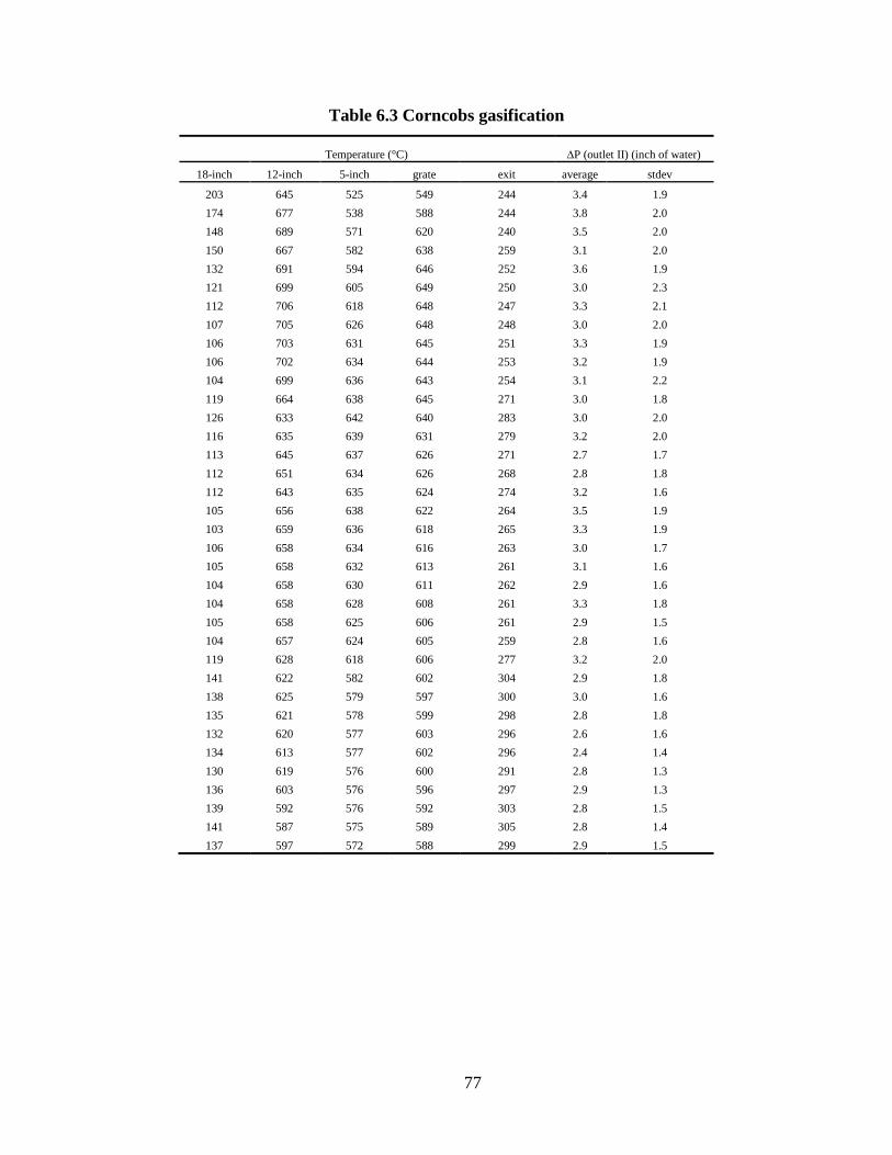
77
Table 6.3 Corncobs gasification
Temperature (°C) ∆P (outlet II) (inch of water)
18-inch 12-inch 5-inch grate exit average stdev
203 645 525 549 244 3.4 1.9 174 677 538 588 244 3.8 2.0 148 689 571 620 240 3.5 2.0 150 667 582 638 259 3.1 2.0 132 691 594 646 252 3.6 1.9 121 699 605 649 250 3.0 2.3 112 706 618 648 247 3.3 2.1 107 705 626 648 248 3.0 2.0 106 703 631 645 251 3.3 1.9 106 702 634 644 253 3.2 1.9 104 699 636 643 254 3.1 2.2 119 664 638 645 271 3.0 1.8 126 633 642 640 283 3.0 2.0 116 635 639 631 279 3.2 2.0 113 645 637 626 271 2.7 1.7 112 651 634 626 268 2.8 1.8 112 643 635 624 274 3.2 1.6 105 656 638 622 264 3.5 1.9 103 659 636 618 265 3.3 1.9 106 658 634 616 263 3.0 1.7 105 658 632 613 261 3.1 1.6 104 658 630 611 262 2.9 1.6 104 658 628 608 261 3.3 1.8 105 658 625 606 261 2.9 1.5 104 657 624 605 259 2.8 1.6 119 628 618 606 277 3.2 2.0 141 622 582 602 304 2.9 1.8 138 625 579 597 300 3.0 1.6 135 621 578 599 298 2.8 1.8 132 620 577 603 296 2.6 1.6 134 613 577 602 296 2.4 1.4 130 619 576 600 291 2.8 1.3 136 603 576 596 297 2.9 1.3 139 592 576 592 303 2.8 1.5 141 587 575 589 305 2.8 1.4 137 597 572 588 299 2.9 1.5

78
Table 6.4 Woodchips gasification
Temperature (°C) ∆P (outlet II) (inch of water)
18-inch 12-inch 5-inch grate exit average stdev
230 482 603 602 247 3.6 2.2 200 680 622 620 252 4.0 2.1 183 755 641 636 258 4.1 2.2 197 740 641 646 293 4.0 2.4 172 757 656 648 282 3.9 1.8 143 804 665 648 267 3.3 2.0 127 786 674 650 267 3.8 2.2 135 736 680 652 276 3.6 2.4 137 738 683 656 282 4.5 2.2 133 745 685 652 285 3.9 2.4 138 734 686 648 289 3.8 2.4 141 709 687 649 294 3.2 2.0 132 720 687 648 287 4.0 2.1 137 707 686 648 294 3.5 2.0 146 685 686 647 304 3.9 2.2 129 711 685 645 286 3.6 2.5 122 715 683 643 278 3.8 2.2 139 689 682 641 289 3.4 2.2 154 689 680 639 291 3.5 2.3 176 694 678 638 296 3.6 2.0 231 687 677 639 313 3.8 1.8 275 695 675 638 318 3.4 2.2 286 680 673 636 323 4.2 2.3 274 649 668 638 330 4.2 2.5 258 631 655 627 335 3.5 2.2 233 654 642 624 322 3.5 2.2 221 661 639 621 313 3.5 2.1 235 656 632 617 316 3.4 2.2 285 660 627 615 322 3.0 2.3 350 657 623 614 333 4.1 2.5 460 643 619 618 351 3.4 2.7 481 634 616 614 350 3.7 2.2

79
Table 6.5 Pressure drop comparison (unit: inch of water)
inlet 18-inch 12-inch grate exit outlet I outlet II
average stdev average stdev average stdev average stdev average stdev average stdev average stdev
no feed
90V -0.42 0.13 -0.36 0.14 -0.36 0.14 -0.36 0.13 -0.37 0.13 3.13 0.89 3.08 0.73 100V -0.55 0.18 -0.53 0.17 -0.51 0.16 -0.51 0.19 -0.53 0.14 4.67 0.90 4.62 0.80 110V -0.56 0.22 -0.49 0.25 -0.46 0.22 -0.48 0.21 -0.53 0.19 4.86 1.20 4.83 1.19 120V -0.58 0.27 -0.53 0.26 -0.48 0.28 -0.53 0.26 -0.54 0.27 4.56 1.60 4.77 1.55
woodchips
90V 0.03 0.08 0.00 0.09 0.01 0.10 -0.05 0.08 -0.04 0.09 1.12 0.47 1.27 0.44 100V -0.09 0.12 -0.08 0.11 -0.12 0.12 -0.26 0.11 -0.30 0.15 2.43 0.54 2.38 0.58 110V -0.18 0.12 -0.22 0.13 -0.27 0.12 -0.46 0.12 -0.54 0.15 3.94 0.82 3.76 0.80 120V -0.30 0.13 -0.34 0.16 -0.38 0.17 -0.65 0.16 -0.76 0.21 4.75 1.07 4.79 1.19
corncobs
90V -0.03 0.09 -0.05 0.09 -0.16 0.11 -0.73 0.18 -0.83 0.19 0.90 0.46 0.87 0.44 100V -0.22 0.10 -0.31 0.11 -0.43 0.14 -1.28 0.18 -1.34 0.11 1.91 0.54 1.78 0.50 110V -0.44 0.14 -0.57 0.15 -0.74 0.18 -1.40 0.06 -1.40 0.07 2.87 0.66 2.82 0.71 120V -0.55 0.22 -0.65 0.23 -0.79 0.27 -1.37 0.09 -1.37 0.10 3.30 1.11 3.07 0.97
DDGS
90V 0.08 0.08 -0.27 0.12 -0.55 0.21 -1.40 0.08 -1.38 0.12 0.31 0.56 0.29 0.60 100V 0.07 0.08 -0.60 0.12 -1.14 0.20 -1.43 0.06 -1.42 0.06 0.43 0.66 0.49 0.55 110V 0.03 0.09 -0.97 0.12 -1.42 0.07 -1.42 0.06 -1.42 0.06 0.71 0.80 0.79 0.62 120V 0.03 0.10 -0.99 0.19 -1.43 0.06 -1.41 0.06 -1.43 0.06 0.93 0.93 0.75 0.97

80
Appendix D - Data Table for Experiment Documentation
Table 6.6 Test and analysis log for gasification experiment
Sampling of Tar in Syngas
Gasifier type:
Test #: Location/Date:
Feedstocks:
Particulate filter temperature (°C):
Weight of flask (g): Weight of sampling bottles (g):
Solvent for tar:
Solvent from T&P sampling:
Solvent from Soxhlet extraction:
Sampling start: Sampling end:
Total sampling duration (hr):
Gas flow rate (L/min):
Total amount of gas sampled (L):
Total tar mass (mg):
Drying temperature (°C): Drying duration (hr):
Remarks:

81
Appendix E - DDGS Properties Analysis
Table 6.7 DDGS properties (data provided by Land O'Lakes Purina Feed) Midwest Sample # Date Sampled
Date Reported QC Sample # Moisture Protein Fat Pro+Fat
L Value
Total Starch
9340606 1/09/08 Wed 1/15/2008 08-0001 11.9 25.0 9.81 34.8 50.8 4.61 9344760 1/28/08 Mon 2/1/2008 08-0004 11.73 27.9 9.7 37.6 52.0 2.69 9345473 1/30/08 Wed 2/5/2008 08-0005 11.51 26.9 8.12 35.0 54.7 4.05 9355598 3/12/08 Wed 3/18/2008 08-0016 12.73 27.5 9.65 37.2 45.0 7.7 9357289 3/19/08 Wed 3/25/2008 08-0017 11.31 28.6 9.9 38.5 48.3 4.84 9358665 3/25/08 Tues 4/1/2008 08-0018 11.94 25.7 10.3 36.0 49.6 5.61 9361023 4/3/2008 Thurs 4/10/2008 08-0021 11.77 27.8 9.69 37.5 50.6 3.63 9362671 4/10/2008 Thurs 4/16/2008 08-0022 12.23 25.9 9.75 35.7 51.0 4.48 9364416 4/16/08 Wed 4/22/2008 08-0025 11.73 25.7 9.78 35.5 51.0 5.43 9366661 4/24/08 Thurs 4/30/2008 08-0026 11.57 26.5 9.69 36.2 49.5 4.35 9366688 4/24/08 Thurs 4/30/2008 Rick's Sample 10.51 28.5 9.38 37.9 Averages 11.72 26.91 9.62 36.52 50.25 4.74
Profat 36.52

82
Appendix F - Biomass Properties (Gaur and Reed, 1998)
Name Proximate analysis Ultimate analysis
Fixed carbon (%) Volatiles (%) Ash (%) HHV (kJ/g) C (%) H (%) O (%) N (%) S (%)
Wood Beech - - 0.65 20.38 51.64 6.26 41.45 0 0
Black Locust 18.26 80.94 0.8 19.71 50.73 5.71 41.93 0.57 0.01 Douglas Fir 17.7 81.5 0.8 21.05 52.3 6.3 40.5 0.1 0
Hickory - - 0.73 20.17 47.67 6.49 43.11 0 0 Maple - - 1.35 19.96 50.64 6.02 41.74 0.25 0
Pinus pinaster 17.17 82.54 0.5 18.4 49.25 5.99 44.36 0.06 0.03 Poplar - - 0.65 20.75 51.64 6.26 41.45 0 0
Red Alder 12.5 87.1 0.4 19.3 49.55 6.06 43.78 0.13 0.07 Redwood 16.1 83.5 0.4 21.03 53.5 5.9 40.3 0.1 0
Western Hemlock 15.2 84.8 2.3 20.05 50.4 5.8 41.1 0.1 0.1 Yellow Pine - - 1.31 22.3 52.6 7 40.1 0 0
White Fir 16.58 83.17 0.25 19.95 49 5.89 44.75 0.05 0.01 White Oak 17.2 81.28 1.52 19.42 49.48 5.38 43.13 0.35 0.01 Madrone 12 87.8 0.2 19.51 48.94 6.03 44.75 0.05 0.02
Mango Wood 11.36 85.64 2.98 19.17 46.24 6.08 44.42 0.28
Bark
Douglas Fir bark 25.8 73 1.2 22.1 56.2 5.9 36.7 0 0 Loblolly Pine bark 33.9 54.7 0.4 21.78 56.3 5.6 37.7 0 0
Energy Crops Eucalyptus camaldulensis 17.82 81.43 0.76 19.42 49 5.87 43.97 0.3 0.01
Casuarina 19.58 78.58 1.83 18.77 48.5 6.04 43.32 0.31 0 Poplar 16.35 82.32 1.33 19.38 48.45 5.85 43.69 0.47 0.01
Sudan Grass 18.6 72.75 8.56 17.39 44.58 5.35 39.18 1.21 0.01
Processed Biomass Plywood 15.77 82.14 2.09 18.96 48.13 5.87 42.46 1.45 0
Agricultural
Peach Pits 19.85 79.12 1.03 20.82 53 5.09 39.14 0.33 0.05 Walnut Shells 21.16 78.28 0.56 20.18 49.48 5.71 43.35 0.21 0.01
Almond Prunings 21.54 76.83 1.63 20.01 51.3 5.27 4.09 0.66 0.01 Black Walnut Prunings 18.56 80.69 0.78 19.83 49.8 5.82 43.23 0.22 0.01
Corncobs 18.54 80.1 1.36 18.77 46.58 5.87 45.46 0.47 0.01 Wheat Straw 19.8 71.3 8.9 17.51 43.2 5 39.4 0.61 0.11 Cotton Stalk 22.43 70.89 6.68 18.26 43.64 5.81 43.87 0 0 Corn Stover 19.25 75.17 5.58 17.65 43.65 5.56 43.31 0.61 0.01
Sugarcane Bagasse 14.95 73.78 11.27 17.33 44.8 5.33 39.55 0.38 0.01 Rice Hulls 15.8 63.6 20.6 14.89 38.3 4.36 35.45 0.83 0
Pine needles 26.12 72.38 1.5 20.12 48.21 6.57 43.72 - 0 Cotton gin trash 15.1 67.3 17.6 16.42 39.59 5.26 36.38 2.09 0

83
Appendix G - Relative Heating Value of Wood as a Function of
Moisture Content
Table 6.8 The relative heating value of wood as a function of moisture content
Moisture (%) 0 a 10 25 50 75 100
Heating value (%) 100 b 90 78 63 52 44
aMoisture content is the weight of moisture as a percentage of wood oven-dry weight for a fixed weight of green wood bHeating value is the amount of usable heat produced by wood at a given moisture content compared with that produced by oven dry wood.
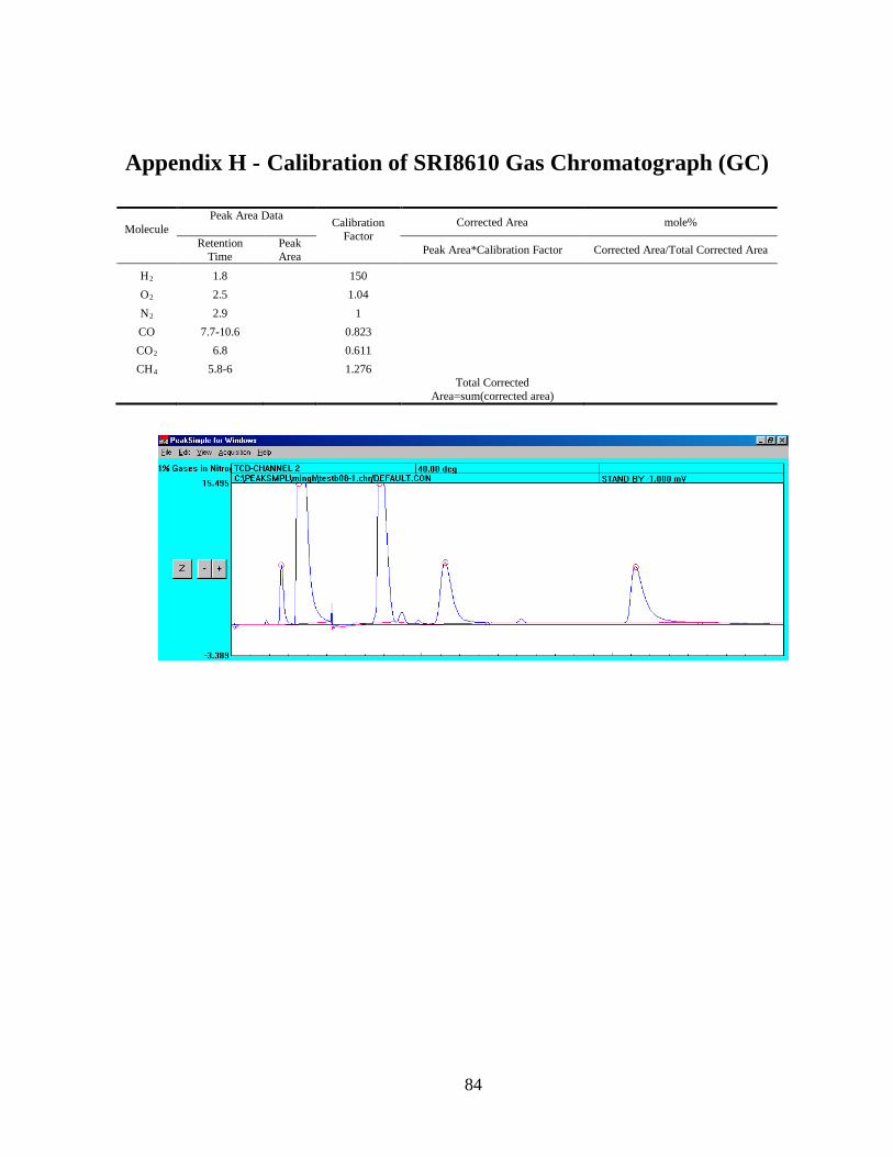
84
Appendix H - Calibration of SRI8610 Gas Chromatograph (GC)
Molecule
Peak Area Data Calibration
Factor
Corrected Area mole%
Retention Time
Peak Area Peak Area*Calibration Factor Corrected Area/Total Corrected Area
H 1.8 2 150 O 2.5 2 1.04 N 2.9 2 1 CO 7.7-10.6 0.823 CO 6.8 2 0.611 CH 5.8-6 4 1.276
Total Corrected
Area=sum(corrected area)
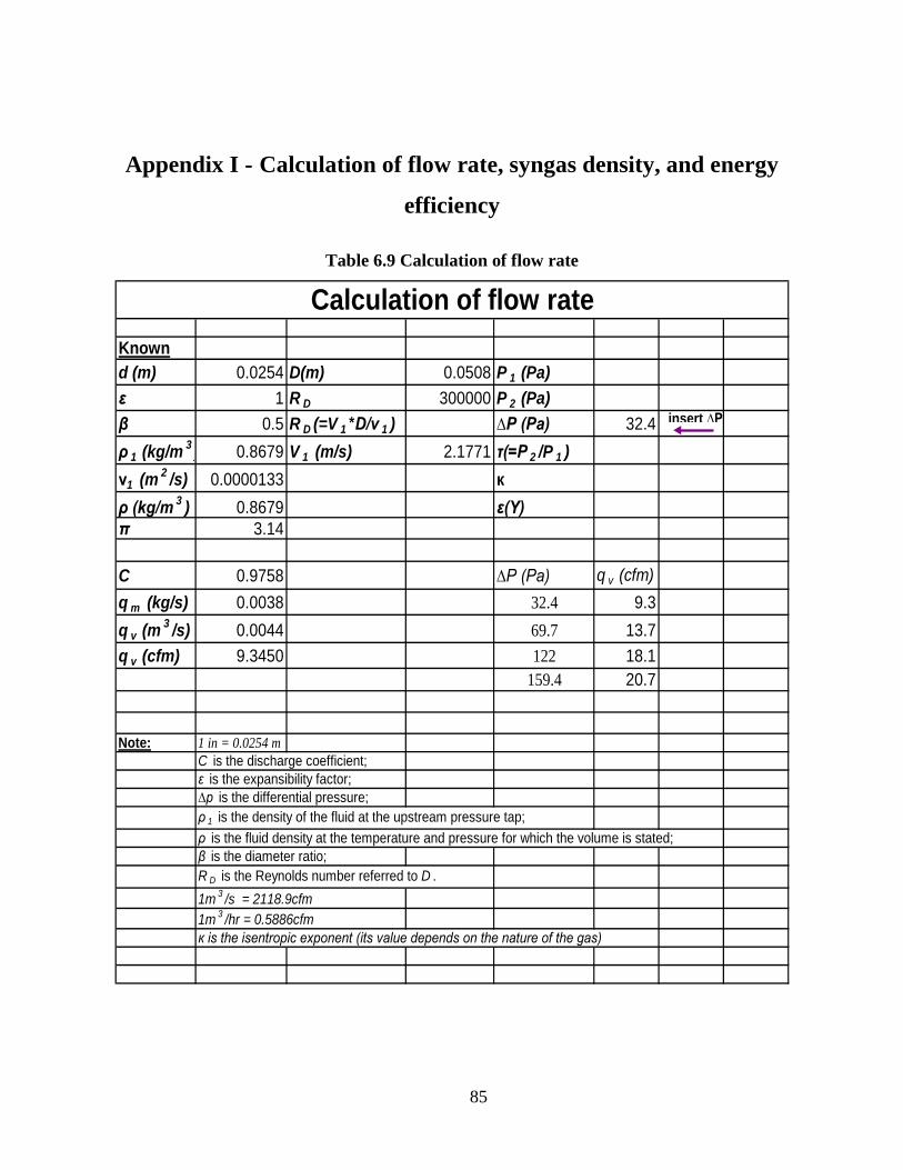
85
Appendix I - Calculation of flow rate, syngas density, and energy
efficiency
Table 6.9 Calculation of flow rate
Knownd (m) 0.0254 D(m) 0.0508 P 1 (Pa)ε 1 R D 300000 P 2 (Pa)β 0.5 R D (=V 1 *D/ν 1 ) ∆P (Pa) 32.4ρ 1 (kg/m 3 ) 0.8679 V 1 (m/s) 2.1771 τ(=P 2 /P 1 )ν1 (m 2 /s) 0.0000133 кρ (kg/m 3 ) 0.8679 ε(Y)π 3.14
C 0.9758 ∆P (Pa) q v (cfm)q m (kg/s) 0.0038 32.4 9.3q v (m
3 /s) 0.0044 69.7 13.7q v (cfm) 9.3450 122 18.1
159.4 20.7
Note: 1 in = 0.0254 mC is the discharge coefficient;ε is the expansibility factor;∆p is the differential pressure;ρ 1 is the density of the fluid at the upstream pressure tap;ρ is the fluid density at the temperature and pressure for which the volume is stated;β is the diameter ratio;R D is the Reynolds number referred to D .1m 3 /s = 2118.9cfm1m 3 /hr = 0.5886cfmк is the isentropic exponent (its value depends on the nature of the gas)
Calculation of flow rate
insert ∆P

86
Table 6.10 Calculation of syngas density
Physical properties of gasesDensity of gases at standard temperature and pressure (0 o C, 1atm):
ρ air (kg/m 3 ) 1.29
ρ H2 (kg/m 3 ) 0.0899
ρ N2 (kg/m 3 ) 1.251
ρ O2 (kg/m 3 ) 1.429
ρ CO (kg/m 3 ) 1.25
ρ CO2 (kg/m 3 ) 2.16
ρ CH4 (kg/m 3 ) 0.783
Density of gases at gasification temperature (49 o C) is calculated based on ideal gas law (ρ=P/R*T):The density of gases at 49 o C, 1atm:
ρ' air (kg/m 3 ) 1.094
ρ' H2 (kg/m 3 ) 0.076
ρ' N2 (kg/m 3 ) 1.061
ρ' O2 (kg/m 3 ) 1.212
ρ' CO (kg/m 3 ) 1.060
ρ' CO2 (kg/m 3 ) 1.831
ρ' CH4 (kg/m 3 ) 0.664
Based on the syngas composition of woodchips gasification: H 2 20.04%O 2 3.15%N 2 61.64%CO 2 0.04%CO 15.01%CH 4 0.12%
ρ syngas (kg/m 3 ) 0.8679
Note: R = 8.314472 m3Pa*K−1*mol−1
0oC = 273.15K
Calculation of syngas density
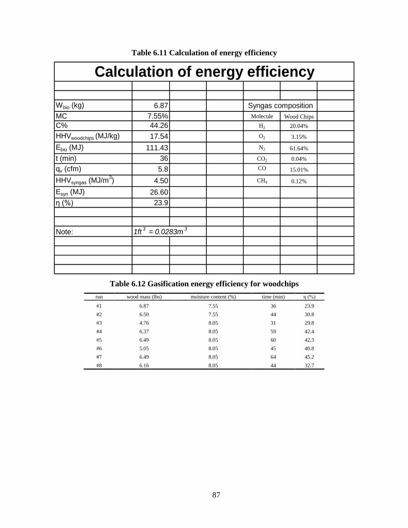
87
Table 6.11 Calculation of energy efficiency
Wbio (kg) 6.87MC 7.55% Molecule Wood ChipsC% 44.26 H2 20.04%
HHVwoodchips (MJ/kg) 17.54 O2 3.15%
Ebio (MJ) 111.43 N2 61.64%
t (min) 36 CO2 0.04%
qv (cfm) 5.8 CO 15.01%
HHVsyngas (MJ/m3) 4.50 CH4 0.12%
Esyn (MJ) 26.60η (%) 23.9
Note: 1ft 3 = 0.0283m 3
Syngas composition
Calculation of energy efficiency
Table 6.12 Gasification energy efficiency for woodchips
run wood mass (lbs) moisture content (%) time (min) η (%)
#1 6.87 7.55 36 23.9 #2 6.50 7.55 44 30.8 #3 4.76 8.05 31 29.8 #4 6.37 8.05 59 42.4 #5 6.49 8.05 60 42.3 #6 5.05 8.05 45 40.8 #7 6.49 8.05 64 45.2 #8 6.16 8.05 44 32.7
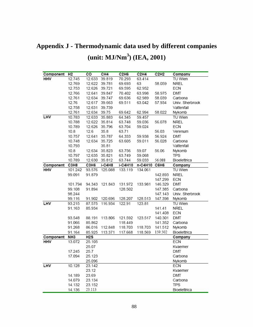
88
Appendix J - Thermodynamic data used by different companies
(unit: MJ/Nm3) (IEA, 2001)