instructors solutions manual for linear and nonlinear ... manual.pdf · paul e. fishback...
TRANSCRIPT

Paul E. Fishback
Instructors Solutions Manualfor Linear and NonlinearProgramming with Maple:An Interactive,Applications-Based Approach

ii
Contents
I Linear Programming 1
1 An Introduction to Linear Programming 31.1 The Basic Linear Programming Problem Formulation . . . . . 41.2 Linear Programming: A Graphical Perspective in R2 . . . . . 101.3 Basic Feasible Solutions . . . . . . . . . . . . . . . . . . . . . . 19
2 The Simplex Algorithm 292.1 The Simplex Algorithm . . . . . . . . . . . . . . . . . . . . . . 302.2 Alternative Optimal/Unbounded Solutions and Degeneracy . 352.3 Excess and Artificial Variables: The Big M Method . . . . . . . 392.4 Duality . . . . . . . . . . . . . . . . . . . . . . . . . . . . . . . . 432.5 Sufficient Conditions for Local and Global Optimal Solutions 542.6 Quadratic Programming . . . . . . . . . . . . . . . . . . . . . . 61
iii

iv

Part I
Linear Programming
1


Chapter 1
An Introduction to Linear Programming
1.1 The Basic Linear Programming Problem Formulation . . . . . . . . . . . . . . . . . . . 4
1.2 Linear Programming: A Graphical Perspective in R2 . . . . . . . . . . . . . . . . . . . . 101.3 Basic Feasible Solutions . . . . . . . . . . . . . . . . . . . . . . . . . . . . . . . . . . . . . . . . . . . . . . . . . . . . . 19
3

4 Chapter 1. An Introduction to Linear Programming
1.1 The Basic Linear Programming Problem Formulation
1. Express each LP below in matrix inequality form. Then solve the LPusing Maple provided it is feasible and bounded.
(a)
maximize z = 6x1 + 4x2
subject to
2x1 + 3x2 ≤ 9
x1 ≥ 4
x2 ≤ 6
x1, x2 ≥ 0,
The second constraint may be rewritten as −x1 ≤ −4 so that matrixinequality form of the LP is given by
maximize z = c · x (1.1)
subject to
Ax ≤ b
x ≥ 0,
where A =
2 3−1 00 1
, c =
[6 4
], b =
9−46
, and x =
[x1
x2
].
The solution is given by x =
[4.50
], with z = 27.
(b)
maximize z = 3x1 + 2x2
subject to
x1 ≤ 4
x1 + 3x2 ≤ 15
2x1 + x2 = 10
x1, x2 ≥ 0.
The third constraint can be replaced by the two constraints, 2x1 +
x2 ≤ 10 and −2x1 − x2 ≤ −10. Thus, the matrix inequality form

1.1. The Basic Linear Programming Problem Formulation 5
of the LP is (1.1), with A =
1 01 32 1−2 −1
, c =
[3 2
], b =
41510−10
, and
x =
[x1
x2
].
The solution is given by x =
[34
], with z = 17.
(c)
maximize z = −x1 + 4x2
subject to
−x1 + x2 ≤ 1
x1 + ≤ 3
x1 + x2 ≥ 5
x1, x2 ≥ 0.
The third constraint is identical to −x1 − x2 ≤ −5. The matrix in-
equality form of the LP is (1.1), with A =
−1 11 0−1 −1
, c =
[−1 4
],
b =
13−5
, and x =
[x1
x2
].
The solution is x =
[34
], with z = 13.
(d)
minimize z = −x1 + 4x2
subject to
x1 + 3x2 ≥ 5
x1 + x2 ≥ 4
x1 − x2 ≤ 2
x1, x2 ≥ 0.
To express the LP in matrix inequality form with the goal of maxi-mization, we set
c = −[−1 4
]=
[1 −4
].
The first two constraints may be rewritten as −x1 − 3x2 ≤ −5 and
6 Chapter 1. An Introduction to Linear Programming
−x1 − x2 ≤ −4. The matrix inequality form of the LP becomes (1.1),
with A =
−1 −3−1 −11 −1
, c =
[1 −4
], b =
−5−42
, and x =
[x1
x2
].
The solution is given by x =
[31
], with z = −1.
(e)
maximize z = 2x1 − x2
subject to
x1 + 3x2 ≥ 8
x1 + x2 ≥ 4
x1 − x2 ≤ 2
x1, x2 ≥ 0.
The first and second constraints are identical to −x1 − 3x2 ≤ −8
and −x1 − x2 ≤ −4, respectively. Thus, A =
−1 −3−1 −11 −1
, c =
[2 −1
],
b =
−8−42
, and x =
[x1
x2
].
The LP is unbounded.
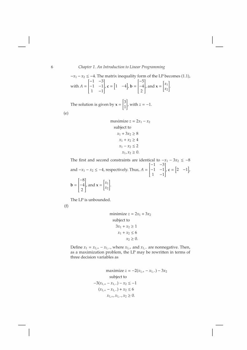
(f)
minimize z = 2x1 + 3x2
subject to
3x1 + x2 ≥ 1
x1 + x2 ≤ 6
x2 ≥ 0.
Define x1 = x1,+ − x1,−, where x1,+ and x1,− are nonnegative. Then,as a maximization problem, the LP may be rewritten in terms ofthree decision variables as
maximize z = −2(x1,+ − x1,−) − 3x2
subject to
−3(x1,+ − x1,−) − x2 ≤ −1
(x1,+ − x1,−) + x2 ≤ 6
x1,+, x1,−, x2 ≥ 0.

1.1. The Basic Linear Programming Problem Formulation 7
The matrix inequality form of the LP becomes (1.1), with A =[−3 3 −11 −1 1
], c =
[−2 2 −3
], b =
[−16
], and x =
x1,+
x1,−x2
.
The solution is given by x1,+ =1
3and x1,− = x2 = 0, with z = −2
3.
2. The LP is given by
minimize z = x1 + 4x2
subject to
x1 + 2x2 ≤ 5
|x1 − x2| ≤ 2
x1, x2 ≥ 0.
The constraint involving the absolute value is identical to −2 ≤ x1−x2 ≤2, which may be written as the two constraints, x1−x2 ≤ 2 and−x1+x2 ≤
2. The matrix inequality form of the LP is (1.1) with A =
1 21 −1−1 1
,
c =[−1 −4
], b =
522
, and x =
[x1
x2
].
The solution is given by x =
[00
], with z = 0.
3. If x1 and x2 denote the number of chairs and number of tables, respec-tively produced by the company, then z = 5x1+7x2 denotes the revenue,which we seek to maximize. The number of square blocks needed toproduce x1 chairs is 2x1, and the number of square blocks needed to pro-duce x2 tables is 2x2. Since six square blocks are available, we have theconstraint, 2x1 + 2x2 ≤ 6. Similar reasoning, applied to the rectangularblocks, leads to the constraint x1 + 2x2 ≤ 8. Along with sign conditions,these results yield the LP
maximize z = 5x1 + 7x2
subject to
2x1 + 2x2 ≤ 6
x1 + 2x2 ≤ 8
x1, x2 ≥ 0.
.
8 Chapter 1. An Introduction to Linear Programming
For the matrix inequality form, A =
[2 21 2
], c =
[5 7
], b =
[68
], and
x =
[x1
x2
].
The solution is given by x =
[03
], with z = 21.
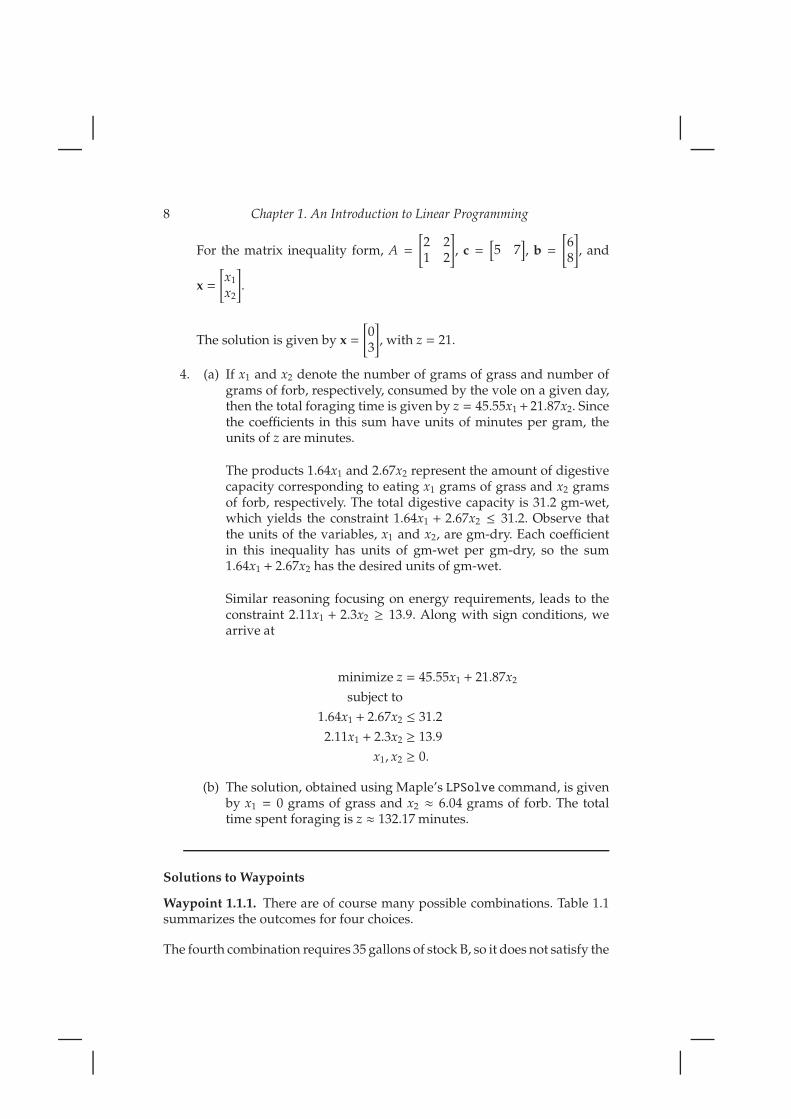
4. (a) If x1 and x2 denote the number of grams of grass and number ofgrams of forb, respectively, consumed by the vole on a given day,then the total foraging time is given by z = 45.55x1+ 21.87x2. Sincethe coefficients in this sum have units of minutes per gram, theunits of z are minutes.
The products 1.64x1 and 2.67x2 represent the amount of digestivecapacity corresponding to eating x1 grams of grass and x2 gramsof forb, respectively. The total digestive capacity is 31.2 gm-wet,which yields the constraint 1.64x1 + 2.67x2 ≤ 31.2. Observe thatthe units of the variables, x1 and x2, are gm-dry. Each coefficientin this inequality has units of gm-wet per gm-dry, so the sum1.64x1 + 2.67x2 has the desired units of gm-wet.
Similar reasoning focusing on energy requirements, leads to theconstraint 2.11x1 + 2.3x2 ≥ 13.9. Along with sign conditions, wearrive at
minimize z = 45.55x1 + 21.87x2
subject to
1.64x1 + 2.67x2 ≤ 31.2
2.11x1 + 2.3x2 ≥ 13.9
x1, x2 ≥ 0.
(b) The solution, obtained using Maple’s LPSolve command, is givenby x1 = 0 grams of grass and x2 ≈ 6.04 grams of forb. The totaltime spent foraging is z ≈ 132.17 minutes.
Solutions to Waypoints
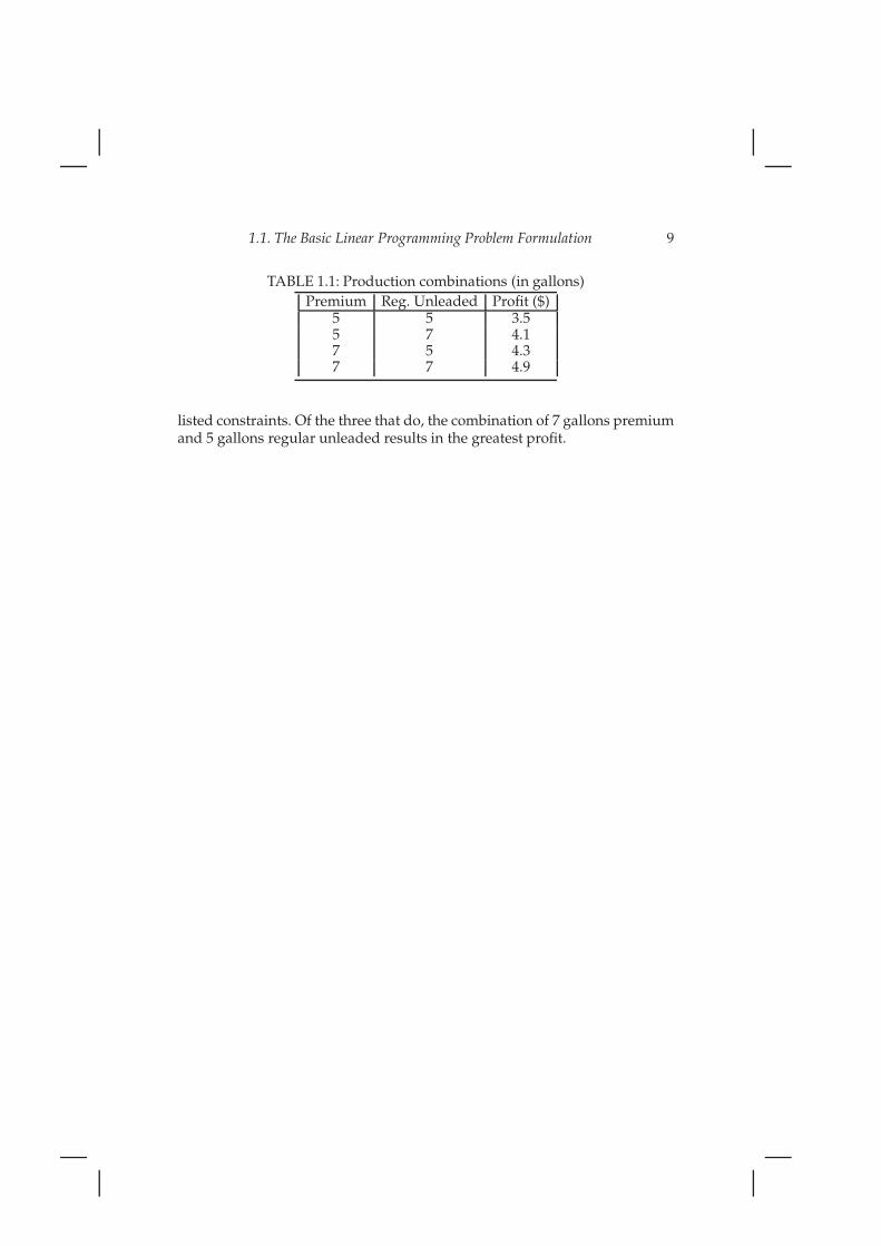
Waypoint 1.1.1. There are of course many possible combinations. Table 1.1summarizes the outcomes for four choices.
The fourth combination requires 35 gallons of stock B, so it does not satisfy the
1.1. The Basic Linear Programming Problem Formulation 9
TABLE 1.1: Production combinations (in gallons)
Premium Reg. Unleaded Profit ($)5 5 3.55 7 4.17 5 4.37 7 4.9
listed constraints. Of the three that do, the combination of 7 gallons premiumand 5 gallons regular unleaded results in the greatest profit.

10 Chapter 1. An Introduction to Linear Programming
1.2 Linear Programming: A Graphical Perspective in R2
1. (a)
Maximize z = 6x1 + 4x2
subject to
2x1 + 3x2 ≤ 9
x1 ≥ 4
x2 ≤ 6
x1, x2 ≥ 0,
The feasible region is shown in Figure 2.2. The solution is given by
x =
[4.50
], with z = 27.
x1
x2
z = 23
z = 25
z = 27
FIGURE 1.1: Feasible region with contours z = 23, z = 25 and z = 27.
1.2. Linear Programming: A Graphical Perspective in R2 11
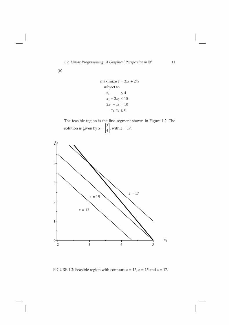
(b)
maximize z = 3x1 + 2x2
subject to
x1 ≤ 4
x1 + 3x2 ≤ 15
2x1 + x2 = 10
x1, x2 ≥ 0.
The feasible region is the line segment shown in Figure 1.2. The
solution is given by x =
[34
], with z = 17.
x1
x2
z = 13
z = 15z = 17
FIGURE 1.2: Feasible region with contours z = 13, z = 15 and z = 17.

12 Chapter 1. An Introduction to Linear Programming
(c)
minimize z = −x1 + 4x2
subject to
x1 + 3x2 ≥ 5
x1 + x2 ≥ 4
x1 − x2 ≤ 2
x1, x2 ≥ 0.
The feasible region is shown in Figure 1.3. The solution is given by
x =
[31
], with z = 1.
x1
x2
z = 5
z = 3
z = 1
FIGURE 1.3: Feasible region with contours z = 5, z = 3 and z = 1.
(d)
maximize z = 2x1 + 6x2
subject to
x1 + 3x2 ≤ 6
x1 + 2x2 ≥ 5
x1, x2 ≥ 0.

1.2. Linear Programming: A Graphical Perspective in R2 13
The feasible region is shown in Figure 1.4. The LP has alternative
optimal solutions that fall on the segment connecting x =
[31
]to
x =
[60
]. Each such solution has an objective value of z = 12, and
the parametric representation of the segment is given by
x =
[3t + 6(1 − t)t + 0(1 − t)
]
=
[6 − 3t
t
],
where 0 ≤ t ≤ 1.
x1
x2
z = 8
z = 10
z = 12
FIGURE 1.4: Feasible region with contours z = 8, z = 10 and z = 12.
14 Chapter 1. An Introduction to Linear Programming
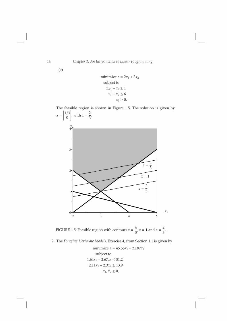
(e)
minimize z = 2x1 + 3x2
subject to
3x1 + x2 ≥ 1
x1 + x2 ≤ 6
x2 ≥ 0.
The feasible region is shown in Figure 1.5. The solution is given by
x =
[1/30
], with z =
2
3.
x1
x2
z =4
3
z = 1
z =2
3
FIGURE 1.5: Feasible region with contours z =4
3, z = 1 and z =
2
3.
2. The Foraging Herbivore Model), Exercise 4, from Section 1.1 is given by
minimize z = 45.55x1 + 21.87x2
subject to
1.64x1 + 2.67x2 ≤ 31.2
2.11x1 + 2.3x2 ≥ 13.9
x1, x2 ≥ 0,

1.2. Linear Programming: A Graphical Perspective in R2 15
whose feasible region is shown in Figure 1.6. The solution is given by
x ≈[
06.043
], with z ≈ 132.171.
x1
x2
z = 300
z = 200
z = 132.171
FIGURE 1.6: Feasible region with contours z = 300, z = 200 and z = 132.171.
3. (a) The feasible region, along with the contours z = 50, z = 100, andz = 150, is shown in Figure 1.7
(b) If M is an arbitrarily large positive real number, then the set ofpoints falling on the contour z = M satisfies 2x1 − x2 = M, or,equivalently, x2 = 2x1 − M. However, as Figure 1.7 indicates, touse the portion of this line that falls within the feasible region, wemust have x1−x2 ≤ 2. Combining this inequality with 2x1−x2 =Myields x1 ≥M−2. Thus, the portion of the contour z =M belongingto the feasible region consists of the ray,
{(x1, x2) | x1 ≥M − 2 and x2 = 2x1 −M} .
(c) Fix M and consider the starting point on the ray from (b). Then
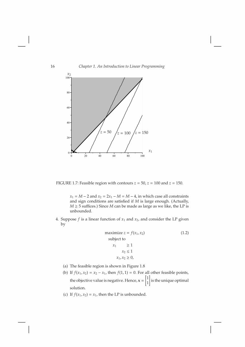
16 Chapter 1. An Introduction to Linear Programming
x1
x2
z = 50 z = 100 z = 150
FIGURE 1.7: Feasible region with contours z = 50, z = 100 and z = 150.
x1 =M− 2 and x2 = 2x1 −M =M − 4, in which case all constraintsand sign conditions are satisfied if M is large enough. (Actually,M ≥ 5 suffices.) Since M can be made as large as we like, the LP isunbounded.
4. Suppose f is a linear function of x1 and x2, and consider the LP givenby
maximize z = f (x1, x2) (1.2)
subject to
x1 ≥ 1
x2 ≤ 1
x1, x2 ≥ 0,
(a) The feasible region is shown in Figure 1.8
(b) If f (x1, x2) = x2 − x1, then f (1, 1) = 0. For all other feasible points,
the objective value is negative. Hence, x =
[11
]is the unique optimal
solution.
(c) If f (x1, x2) = x1, then the LP is unbounded.

1.2. Linear Programming: A Graphical Perspective in R2 17
x1
x2
FIGURE 1.8: Feasible region for LP 1.2.
(d) If f (x1, x2) = x2, then the LP has alternative optimal solutions.
Solutions to Waypoints
Waypoint 1.2.1. The following Maple commands produce the desired feasibleregion:
> restart:with(plots):
> constraints:=[x1<=8,2*x1+x2<=28,3*x1+2*x2<=32,x1>=0,x2>=0]:
> inequal(constraints,x1=0..10,x2=0..16,optionsfeasible=(color=grey),optionsexcluded=(color=white),optionsclosed=(color=black),thickness=1);
Waypoint 1.2.2. The following commands produce the feasible region, uponwhich are superimposed the contours, z = 20, z = 30, and z = 40.
> restart:with(plots):
> f:=(x1,x2)->4*x1+3*x2;
f := (x1, x2)→ 4x1 + 3x2
> constraints:=[x1<=8,2*x1+x2<=28,3*x1+2*x2<=32,x1>=0,x2>=0]:
> FeasibleRegion:=inequal(constraints,x1=0..10,x2=0..16,optionsfeasible=(color=grey),optionsexcluded=(color=white),optionsclosed=(color=black),thickness=2):

18 Chapter 1. An Introduction to Linear Programming
x1
x2
FIGURE 1.9: Feasible region and object contours z = 20, z = 30, and z = 40.
> ObjectiveContours:=contourplot(f(x1,x2),x1=0..10,x2=0..10,contours=[20,30,40],thicknes
> display(FeasibleRegion, ObjectiveContours);
The resulting graph is shown in Figure 1.9Maple does not label the contours, but the contours must increase in value asx1 and x2 increase. This fact, along with the graph, suggests that the solutionis given by x1 = 4, x2 = 10.

1.3. Basic Feasible Solutions 19
1.3 Basic Feasible Solutions
1. For each of the following LPs, write the LP in the standard matrix form
maximize z = c · xsubject to
[A|Im]
[xs
]= b
x, s ≥ 0.
Then determine all basic and basic feasible solutions, expressing eachsolution in vector form. Label each solution next to its correspondingpoint on the feasible region graph.
(a)
Maximize z = 6x1 + 4x2
subject to
2x1 + 3x2 ≤ 9
x1 ≥ 4
x2 ≤ 6
x1, x2 ≥ 0,
Note that this LP is the same as that from Exercise 1a of Section
1.1, where A =
2 3−1 00 1
, c =
[6 4
], b =
9−46
, and x =
[x1
x2
]. Since
there are three constraints, s =
s1
s2
s3
.
In this case, the matrix equation,
[A|Im]
[xs
]= b (1.3)
has at most
(52
)= 10 possible basic solutions. Each is obtained by
setting two of the five entries of
[xs
]to zero and solving (1.3) for
the remaining three, provided the system is consistent. Of the tenpossible cases to consider, two lead to inconsistent systems. Theyarise from setting x1 = s2 = 0 and from setting x2 = s3 = 0. Theeight remaining consistent systems yield the following results:

20 Chapter 1. An Introduction to Linear Programming
i. x1 = 0, x2 = 0, s1 = 9, s2 = −4, s3 = 6 (basic, but not basicfeasible solution)
ii. x1 = 0, x2 = 3, s1 = 0, s2 = −4, s3 = 3 (basic, but not basicfeasible solution)
iii. x1 = 0, x2 = 6, s1 = −9, s2 = −4, s3 = 0 (basic, but not basicfeasible solution)
iv. x1 = 4.5, x2 = 0, s1 = 0, s2 = .5, s3 = 6 (basic feasible solution)
v. x1 = 4, x2 = 0, s1 = 1, s2 = 0, s3 = 6 (basic feasible solution)
vi. x1 = 4, x2 = 1/3, s1 = 0, s2 = 0, s3 = 17/3 (basic feasible solu-tion)
vii. x1 = −4.5, x2 = 6, s1 = 0, s2 = −8.5, s3 = 0 (basic, but not basicfeasible solution)
viii. x1 = 4, x2 = 6, s1 = −17, s2 = 0, s3 = 0 (basic, but not basicfeasible solution)
The feasible region is that from Exercise 1a of Section 1.2, and thesolution is x1 = 4.5 and x2 = 0 with z = 27.
(b)
minimize z = −x1 + 4x2
subject to
x1 + 3x2 ≥ 5
x1 + x2 ≥ 4
x1 − x2 ≤ 2
x1, x2 ≥ 0.
Note that this LP is the same as that from Exercise 1d of Section
1.1, where A =
−1 −3−1 −11 −1
, c =
[1 −4
], b =
−5−42
, and x =
[x1
x2
]Since
there are three constraints, s =
s1
s2
s3
.
As in the previous exercise, there are ten possible cases to consider.In this situation, all ten systems are consistent. The results are asfollows:
i. x1 = 0, x2 = 0, s1 = −5, s2 = −4, s3 = 2 (basic, but not basicfeasible solution)
ii. x1 = 0, x2 = 5/3, s1 = 0, s2 = −7/3, s3 = 11/3 (basic, but notbasic feasible solution)
iii. x1 = 0, x2 = 4, s1 = 7, s2 = 0, s3 = 6 (basic feasible solution)

1.3. Basic Feasible Solutions 21
iv. x1 = 0, x2 = −2, s1 = −11, s2 = −6, s3 = 0 (basic, but not basicfeasible solution)
v. x1 = 5, x2 = 0, s1 = 0, s2 = 1, s3 = −3 (basic, but not basicfeasible solution)
vi. x1 = 4, x2 = 0, s1 = −1, s2 = 0, s3 = −2 (basic, but not basicfeasible solution)
vii. x1 = 2, x2 = 0, s1 = −3, s2 = −2, s3 = 0 (basic, but not basicfeasible solution)
viii. x1 = 7/2, x2 = 1/2, s1 = 0, s2 = 0, s3 = −1 (basic, but not basicfeasible solution)
ix. x1 = 11/4, x2 = 3/4, s1 = 0, s2 = −1/2, s3 = 0 (basic, but notbasic feasible solution)
x. x1 = 3, x2 = 1, s1 = 1, s2 = 0, s3 = 0 (basic feasible solution)
The feasible region is that from Exercise 1c of Section 1.2, and thesolution is x1 = 3 and x2 = 1 with z = 1.
2. The constraint equations of the standard form of the FuelPro LP aregiven by
x1 + s1 = 8 (1.4)
2x1 + 2x2 + s2 = 28
3x1 + 2x2 + s3 = 32
If x1 and s1 are nonbasic, then both are zero. In this case (1.4) is inconsis-tent. Observe that if x1 = s1 = 0, that the coefficient matrix correspond-
ing to (1.4) is given by M =
0 0 02 1 02 0 1
, which is not invertible.
3. The LP is given by
maximize z = 3x1 + 2x2
subject to
x1 ≤ 4
x1 + 3x2 ≤ 15
2x1 + x2 = 10
x1, x2 ≥ 0.
(a) The third constraint is the combination of 2x1 + x2 ≤ 10 and −2x1 −2x2 ≤ −10. Thus, the matrix inequality form of the LP has A =
1 01 32 2−2 −2
and b =
41510−10
.
22 Chapter 1. An Introduction to Linear Programming
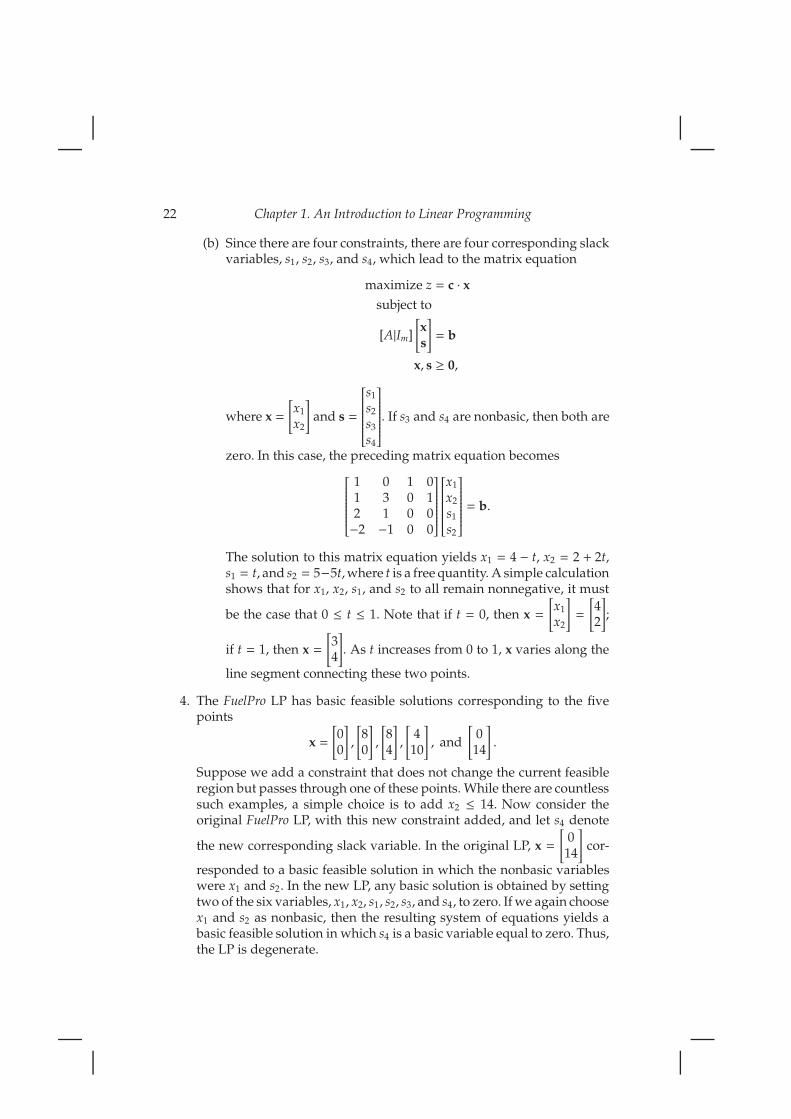
(b) Since there are four constraints, there are four corresponding slackvariables, s1, s2, s3, and s4, which lead to the matrix equation
maximize z = c · xsubject to
[A|Im]
[xs
]= b
x, s ≥ 0,
where x =
[x1
x2
]and s =
s1
s2
s3
s4
. If s3 and s4 are nonbasic, then both are
zero. In this case, the preceding matrix equation becomes
1 0 1 01 3 0 12 1 0 0−2 −1 0 0
x1
x2
s1
s2
= b.
The solution to this matrix equation yields x1 = 4 − t, x2 = 2 + 2t,s1 = t, and s2 = 5−5t, where t is a free quantity. A simple calculationshows that for x1, x2, s1, and s2 to all remain nonnegative, it must
be the case that 0 ≤ t ≤ 1. Note that if t = 0, then x =
[x1
x2
]=
[42
];
if t = 1, then x =
[34
]. As t increases from 0 to 1, x varies along the
line segment connecting these two points.
4. The FuelPro LP has basic feasible solutions corresponding to the fivepoints
x =
[00
],
[80
],
[84
],
[4
10
], and
[0
14
].
Suppose we add a constraint that does not change the current feasibleregion but passes through one of these points. While there are countlesssuch examples, a simple choice is to add x2 ≤ 14. Now consider theoriginal FuelPro LP, with this new constraint added, and let s4 denote
the new corresponding slack variable. In the original LP, x =
[0
14
]cor-
responded to a basic feasible solution in which the nonbasic variableswere x1 and s2. In the new LP, any basic solution is obtained by settingtwo of the six variables, x1, x2, s1, s2, s3, and s4, to zero. If we again choosex1 and s2 as nonbasic, then the resulting system of equations yields abasic feasible solution in which s4 is a basic variable equal to zero. Thus,the LP is degenerate.
1.3. Basic Feasible Solutions 23
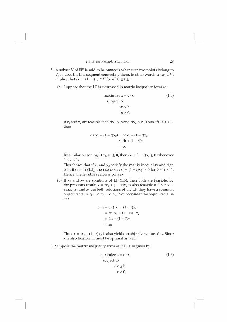
5. A subset V of Rn is said to be convex is whenever two points belong toV, so does the line segment connecting them. In other words, x1, x2 ∈ V,implies that tx1 + (1 − t)x2 ∈ V for all 0 ≤ t ≤ 1.
(a) Suppose that the LP is expressed in matrix inequality form as
maximize z = c · x (1.5)
subject to
Ax ≤ b
x ≥ 0.
If x1 and x2 are feasible then Ax1 ≤ b and Ax2 ≤ b. Thus, if 0 ≤ t ≤ 1,then
A (tx1 + (1 − t)x2) = tAx1 + (1 − t)x2
≤ tb + (1 − t)b
= b.
By similar reasoning, if x1, x2 ≥ 0, then tx1 + (1− t)x2 ≥ 0 whenever0 ≤ t ≤ 1.
This shows that if x1 and x2 satisfy the matrix inequality and signconditions in (1.5), then so does tx1 + (1 − t)x2 ≥ 0 for 0 ≤ t ≤ 1.Hence, the feasible region is convex.
(b) If x1 and x2 are solutions of LP (1.5), then both are feasible. Bythe previous result, x = tx1 + (1 − t)x2 is also feasible if 0 ≤ t ≤ 1.Since, x1 and x2 are both solutions of the LP, they have a commonobjective value z0 = c · x1 = c · x2. Now consider the objective valueat x:
c · x = c · (tx1 + (1 − t)x2)
= tc · x1 + (1 − t)c · x2
= tz0 + (1 − t)z0
= z0.
Thus, x = tx1 + (1− t)x2 is also yields an objective value of z0. Sincex is also feasible, it must be optimal as well.
6. Suppose the matrix inequality form of the LP is given by
maximize z = c · x (1.6)
subject to
Ax ≤ b
x ≥ 0,
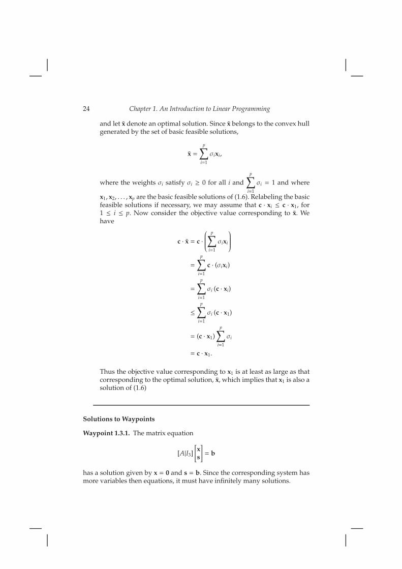
24 Chapter 1. An Introduction to Linear Programming
and let x denote an optimal solution. Since x belongs to the convex hullgenerated by the set of basic feasible solutions,
x =
p∑
i=1
σixi,
where the weights σi satisfy σi ≥ 0 for all i and
p∑
i=1
σi = 1 and where
x1, x2, . . . , xp are the basic feasible solutions of (1.6). Relabeling the basicfeasible solutions if necessary, we may assume that c · xi ≤ c · x1, for1 ≤ i ≤ p. Now consider the objective value corresponding to x. Wehave
c · x = c ·
p∑
i=1
σixi
=
p∑
i=1
c · (σixi)
=
p∑
i=1
σi (c · xi)
≤p∑
i=1
σi (c · x1)
= (c · x1)
p∑
i=1
σi
= c · x1.
Thus the objective value corresponding to x1 is at least as large as thatcorresponding to the optimal solution, x, which implies that x1 is also asolution of (1.6)
Solutions to Waypoints
Waypoint 1.3.1. The matrix equation
[A|I3]
[xs
]= b
has a solution given by x = 0 and s = b. Since the corresponding system hasmore variables then equations, it must have infinitely many solutions.

1.3. Basic Feasible Solutions 25
Waypoint 1.3.2. To solve the given matrix equation, we row reduce the aug-mented matrix
1 0 1 0 02 2 0 1 03 2 0 0 1
∣∣∣∣∣∣∣∣
82832
.
The result is given by
1 0 0 −1 10 1 0 3/2 −10 0 1 1 −1
∣∣∣∣∣∣∣∣
4104
.
If we let s2 and s3 denote the free variables, then we may write s2 = t,s3 = s, where t, s ∈ R. With this notation, x1 = 4 + t − s, x2 = 10 − 3
2 t + s, ands1 = 4 − t + s. We obtain the five extreme points as follows:
1. t = 28 and s = 32 yield x =
[00
]and s =
82832
2. t = 12 and s = 8 yield x =
[80
]and s =
0128
3. t = 4 and s = 0 yield x =
[84
]and s =
040
4. t = s = 0 yields x =
[4
10
]and s =
400
5. t = 0 and s = 4 yield x =
[0
14
]and s =
804
These extreme points may then be labeled on the feasible region.
Waypoint 1.3.3. 1. The feasible region and various contours are shown inFigure ??
The extreme points are given by the x1 =
[00
], x2 =
[3/20
], x3 =
[6/712/7
],
and x4 =
[04
].
2. If c = [−5, 2], A =
[3 28 3
], b =
[612
], x =
[x1
x2
], and s =
[s1
s2
], then the
standard matrix form is given by

26 Chapter 1. An Introduction to Linear Programming
x1
x2 z = 0
z = −3
z = −5
z = −7.5
FIGURE 1.10: Feasible region with contours z = 0, z = −3, z = −5 andz = −7.5.
maximize z = c · xsubject to
[A|I2]
[xs
]= b
x, s ≥ 0,
3. The two constraint equations can be expressed as 3x1 + 2x2 = 6 and8x1 + 3x2 = 12. Substituting x1 = x2 = 0 into this equations yieldsthe basic solution x1 = 0, x2 = 0, s1 = 6 and s2 = 16. Performing thesame operations using the other three extreme points from (1) yieldsthe remaining three basic feasible solutions:
(a) x1 = 1.5, x2 = 0, s1 = 1.5 and s2 = 0

1.3. Basic Feasible Solutions 27
(b) x1 =67 , x2 =
127 , s1 = 0 and s2 = 0
(c) x1 = 0, x2 = 3, s1 = 0 and s2 = 16
4. The contours in Figure ?? indicate the optimal solution occurs at the
basic feasible solution x =
[1.50
], where z = −7.5.

28 Chapter 1. An Introduction to Linear Programming
Chapter 2
The Simplex Algorithm
2.1 The Simplex Algorithm . . . . . . . . . . . . . . . . . . . . . . . . . . . . . . . . . . . . . . . . . . . . . . . . . . . . . 302.2 Alternative Optimal/Unbounded Solutions and Degeneracy . . . . . . . . . . . 352.3 Excess and Artificial Variables: The Big M Method . . . . . . . . . . . . . . . . . . . . . . 392.4 Duality . . . . . . . . . . . . . . . . . . . . . . . . . . . . . . . . . . . . . . . . . . . . . . . . . . . . . . . . . . . . . . . . . . . . . . . 432.5 Sufficient Conditions for Local and Global Optimal Solutions . . . . . . . . . . 542.6 Quadratic Programming . . . . . . . . . . . . . . . . . . . . . . . . . . . . . . . . . . . . . . . . . . . . . . . . . . . . 61
29

30 Chapter 2. The Simplex Algorithm
2.1 The Simplex Algorithm
1. For each LP, we indicate the tableau after each iteration and highlightthe pivot entry used to perform the next iteration.
(a)
TABLE 2.1: Initial tableauz x1 x2 s1 s2 s3 RHS1 -3 -2 0 0 0 0
0 1 0 1 0 0 40 1 3 0 1 0 150 2 1 0 0 1 10
TABLE 2.2: Tableau after first iterationz x1 x2 s1 s2 s3 RHS1 0 -2 3 0 0 120 1 0 1 0 0 40 0 3 -1 1 0 11
0 0 1 -2 0 1 2
TABLE 2.3: Tableau after second iterationz x1 x2 s1 s2 s3 RHS1 0 0 -1 0 2 160 1 0 1 0 0 4
0 0 0 5 1 -3 50 0 1 -2 0 1 2
The solution is x1 = 3 and x2 = 4, with z = 17.
(b)

2.1. The Simplex Algorithm 31
TABLE 2.4: Final tableauz x1 x2 s1 s2 s3 RHS1 0 0 0 1/5 7/5 170 1 0 0 -1/5 3/5 30 0 0 1 1/5 -3/5 10 0 1 0 2/5 -1/5 4
TABLE 2.5: Initial tableauz x1 x2 s1 s2 s3 RHS1 -4 -3 0 0 0 0
0 1 0 1 0 0 40 -2 1 0 1 0 120 1 2 0 0 1 14
The solution is x1 = 4 and x2 = 5, with z = 31.
(c)
The solution is x1 = 2, x2 = 0, and x3 =10
3, with z =
74
3.
(d)
This is a minimization problem, so we terminate the algorithmwhen all coefficients in the top row that correspond to nonbasicvariables are nonpositive. The solution is x1 = 0 and x2 = 4, withz = −8.
2. If we rewrite the first and second constraints as −x1 − 3x2 ≤ −8 and−x1−x2 ≤ −4 and incorporate slack variables as usual, our initial tableaubecomes that shown in Table 2.13
The difficulty we face when attempting to perform the simplex algo-rithm, centers on the fact that the origin, (x1, x2) = (0, 0) yields negativevalues of s1 and 2. In other words, the origin corresponds to a basic, butnot basic feasible, solution. We cannot read off the initial basic feasiblesolution as we could for Exercise (1d).
3. We list those constraints that are binding for each LP.
(a) Constraints 2 and 3

32 Chapter 2. The Simplex Algorithm
TABLE 2.6: Tableau after first iterationz x1 x2 s1 s2 s3 RHS1 0 -3 4 0 0 160 1 0 1 0 0 40 0 1 2 1 0 20
0 0 2 -1 0 1 10
TABLE 2.7: Final tableauz x1 x2 s1 s2 s3 RHS1 0 0 5/2 0 3/2 310 1 0 1 0 0 40 0 0 5/2 1 -1/2 150 0 1 -1/2 0 1/2 5
(b) Constraints 1 and 3
(c) Constraints 1 and 2
(d) Constraint 2
Solutions to Waypoints
Waypoint 2.1.1. We first state the LP in terms of maximization. If we setz = −z, then
maximize z = 5x1 − 2x2 (2.1)
subject to
x1 ≤ 2
3x1 + 2x2 ≤ 6
8x1 + 3x2 ≤ 12
x1, x2 ≥ 0,
where z = −z.The initial tableau corresponding to LP (2.1) is given bySince we are now solving a maximization problem, we pivot on the high-lighted entry in this tableau, which yields the following:All entries in the top row corresponding to nonbasic variables are positive.Hence x1 =
32 and x2 = 0 is a solution of the LP. However, the objective
value corresponding to this optimal solution, for the original LP, is given byz = −z = − 15
2 .
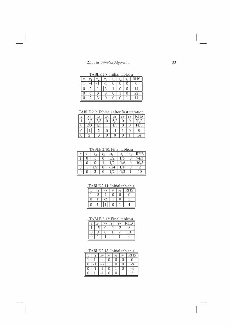
2.1. The Simplex Algorithm 33
TABLE 2.8: Initial tableauz x1 x2 x3 s1 s2 s3 RHS1 -4 -1 -5 0 0 0 0
0 2 1 3 1 0 0 140 6 3 3 0 1 0 220 2 3 0 0 0 1 14
TABLE 2.9: Tableau after first iterationz x1 x2 x3 s1 s2 s3 RHS1 -2/3 2/3 0 5/3 0 0 70/30 2/3 1/3 1 1/3 0 0 14/3
0 4 2 0 -1 1 0 80 2 3 0 0 0 1 14
TABLE 2.10: Final tableauz x1 x2 x3 s1 s2 s3 RHS1 0 1 0 3/2 1/6 0 74/30 0 0 1 1/2 -1/6 0 10/30 1 1/2 0 -1/4 1/4 0 20 0 2 0 1/2 -1/2 1 10
TABLE 2.11: Initial tableauz x1 x2 s1 s2 RHS1 -3 2 0 0 00 1 -2 1 0 2
0 1 1 0 1 4
TABLE 2.12: Final tableauz x1 x2 s1 s2 RHS1 -5 0 0 -2 -80 3 0 1 2 100 1 1 0 1 4
TABLE 2.13: Initial tableauz x1 x2 s1 s2 s3 RHS1 1 -4 0 0 0 00 -1 -3 1 0 0 -80 -1 -1 0 1 0 -40 1 -1 0 0 1 2

34 Chapter 2. The Simplex Algorithm
TABLE 2.14: Initial tableauz x1 x2 s1 s2 s3 RHS1 -5 2 0 0 0 00 1 0 1 0 0 20 3 2 0 1 0 6
0 8 3 0 0 1 12
TABLE 2.15: Final tableauz x1 x2 s1 s2 s3 RHS1 0 31/8 0 0 5/8 15/20 0 -3/8 1 0 -1/8 1/20 0 7/8 0 1 -3/8 3/20 1 3/8 0 0 1/8 3/2

2.2. Alternative Optimal/Unbounded Solutions and Degeneracy 35
2.2 Alternative Optimal/Unbounded Solutions and Degen-eracy
1. Exercise 1
The initial tableau is shown in Table
TABLE 2.16: Initial tableau for Exercise 1z x1 x2 s1 s2 RHS1 -2 -6 0 0 00 1 3 1 0 60 0 1 0 1 1
After performing two iterations of the simplex algorithm, we obtain thefollowing:
TABLE 2.17: Tableau after second iteration for Exercise 1z x1 x2 s1 s2 RHS1 0 0 2 0 120 1 0 1 -3 3
0 0 1 0 1 1
At this stage, the basic variables are x1 = 3 and x2 = 1, with a correspond-ing objective value z = 12. The nonbasic variable, s2, has a coefficient ofzero in the top row. Thus, letting s2 become basic will not change thevalue of z. In fact, if we pivot on the highlighted entry in Table 2.17,x2 replaces s2 as a nonbasic variable, x1 = 6, and the objective value isunchanged.
2. Exercise 2 For an LP minimization problem to be unbounded, there must
exist, at some stage of the simplex algorithm, a basic feasible solutionin which a nonbasic variable has a negative coefficient in the top rowand nonpositive coefficients in the remaining rows.
3. Exercise 3
(a) For the current basic solution to not be optimal, it must be the casethat a < 0. However, if the LP is bounded, then the ratio test forcesb > 0. Thus, we may pivot on row and column containing b, inwhich case, we obtain the following tableau:

36 Chapter 2. The Simplex Algorithm
TABLE 2.18: Tableau obtained after pivoting on row and column containingb
z x1 x2 s1 s2 RHS1 0 − a
b 0 3 − ab 10 − 2 a
b
0 1 1b 0 1
b − 1 3 + 2b
0 0 1b 1 1
b2b
Thus, x1 = 3 +2
b, x2 = 0, and z = 10 − 2
a
b.
(b) If the given basic solution was optimal, then a ≥ 0. However, ifthe LP has alternative optimal solutions, then a = 0. In this case,pivoting on the same entry in the original tableau as we did in(b), we would obtain the result in Table 2.18, but with a = 0. Thus,
x1 = 3 +2
b, x2 = 0, and z = 10.
(c) If the LP is unbounded, then a < 0 and b ≤ 0.
4. Exercise 4
(a) The coefficient of the nonbasic variable, s1, in the top row of thetableau is negative. Since the coefficient of s1 in the remaining tworows is also negative, we see that the LP is unbounded.
(b) So long as s2 remains non basic, the equations relating s1 to eachof x1 and x2 are given by x1 − 2s1 = 4 and x2 − s1 = 5. Thus, foreach unit of increase in s1, x1 increases by 2 units; for each unit ofincrease in s1, x2 increases by 1 unit.
(c) Eliminating s1 from the equations x1 − 2s1 = 4 and x2 − s1 = 5, we
obtain x2 =1
2x1 + 3.
(d) When s1 = 0, x1 = 4 and x2 = 5. Since s1 ≥ 0, x1 ≥ 4 and x2 ≥ 5.
Thus,we sketch that portion of the line x2 =1
2x1 + 3 for which
x1 ≥ 4 and x2 ≥ 5.
(e) Since z = 1, 000, z = x1 + 3x2, and x2 =1
2x1 + 3, we have a system
of equations whose solution is given by x1 =1982
5and x2 =
1006
5.
5. Exercise 5
(a) The LP has 2 decision variables and 4 constraints. Inspection of the

2.2. Alternative Optimal/Unbounded Solutions and Degeneracy 37
graph shows that the constraints are given by
2x1 + x2 ≤ 10
x1 + x2 ≤ 6
1
2x1 + x2 ≤ 4
−1
2x1 + x2 ≤ 2.
By introducing slack variables, s1, s2, s3, and s4, we can convertthe preceding list of inequalities to a system of equations in sixvariables, x1, x2, s1, s2, s3, and s4. Basic feasible solutions are thenmost easily determined by substituting each of the extreme pointsinto the system of equations and solving for the slack variables.The results are as follows:
[xs
]=
00
10642
=
5011
3/29/2
=
420002
=
233100
=
028420
Observe that the extreme point x =
[42
]yields slack variable values
for which s1 = s2 = s3 = 0. This means that when any two of thesethree variables are chosen to be nonbasic, the third variable, whichis basic, must be zero. Hence, the LP is degenerate. From a graphicalperspective, the LP is degenerate because the boundaries of three
of the constraints intersect at the single extreme point, x =
[42
]
(b) If the origin is the initial basic feasible solution, at least two simplexalgorithm iterations are required before a degenerate basic feasiblesolution results. This occurs when the objective coefficient of x1 islarger than that of x2. In this case, the intermediate iteration yields
x =
[50
]. If the objective coefficient of x2 is positive and larger than
that of x1, then at most three iterations are required.

38 Chapter 2. The Simplex Algorithm
Solutions to Waypoints
Waypoint 2.2.1. 1. The current basic feasible solution consists of x1 = a,s1 = 2, and x2 = s2 = 0. The LP has alternative optimal solutions if anonbasic variable has a coefficient of zero in the top row of the tableau.This occurs when a = 1 or a = 2.
2. The LP is unbounded if both 1− a < 0 and a− 3 < 0, i.e., if 1 < a ≤ 3. TheLP is also unbounded if both 2 − a < 0 and a − 4 ≤ 0, i.e., if 2 < a ≤ 4.

2.3. Excess and Artificial Variables: The Big M Method 39
2.3 Excess and Artificial Variables: The Big M Method
1. (a) We let e1 and a1 denote the excess and artificial variables, respec-tively, that correspond to the first constraint. Similarly, we let e2
and a2 correspond to the second constraint. Using M = 100, ourobjective becomes one of minimizing z = −x1+ 4x2+ 100a1+ 100a2.If s3 is the slack variable corresponding to the third constraint ourinitial tableau is as follows:
TABLE 2.19: Initial tableauz x1 x2 e1 a1 e2 a2 s3 RHS1 1 -4 0 -100 0 -100 0 0
0 1 3 -1 1 0 0 0 8
0 1 1 0 0 -1 1 0 40 1 -1 0 0 0 0 1 2
To obtain an initial basic feasible solution, we pivot on each of thehighlighted entries in this tableau. The result is the following:
TABLE 2.20: Tableau indicting initial basic feasible solution
z x1 x2 e1 a1 e2 a2 s3 RHS1 201 396 -100 0 -100 0 0 12000 1 3 -1 1 0 0 0 80 1 1 0 0 -1 1 0 40 1 -1 0 0 0 0 1 2
Three iterations of the simplex algorithm are required before all co-efficients in the top row of the tableau that correspond to nonbasicvariables are nonpositive. The final tableau is given by
TABLE 2.21: Final tableauz x1 x2 e1 a1 e2 a2 s3 RHS1 0 0 -3/4 -397/4 0 -100 -7/4 5/20 0 1 -1/4 1/4 0 0 -1/4 3/20 1 0 -1/4 1/4 0 0 3/4 7/20 0 0 -1/2 1/2 1 -1 1/2 1
The solution is x1 =7
2and x2 =
3
2, with x2 =
5
2.
40 Chapter 2. The Simplex Algorithm
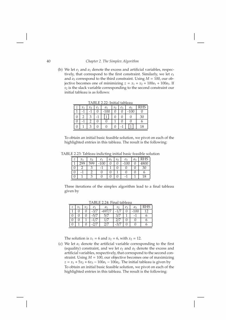
(b) We let e1 and a1 denote the excess and artificial variables, respec-tively, that correspond to the first constraint. Similarly, we let e3
and a3 correspond to the third constraint. Using M = 100, our ob-jective becomes one of minimizing z = x1 + x2 + 100a1 + 100a3. Ifs2 is the slack variable corresponding to the second constraint ourinitial tableau is as follows:
TABLE 2.22: Initial tableauz x1 x2 e1 a1 s2 e3 a3 RHS1 -1 -1 0 -100 0 0 -100 0
0 2 3 -1 1 0 0 0 300 -1 2 0 0 1 0 0 6
0 1 3 0 0 0 -1 1 18
To obtain an initial basic feasible solution, we pivot on each of thehighlighted entries in this tableau. The result is the following:
TABLE 2.23: Tableau indicting initial basic feasible solution
z x1 x2 e1 a1 s2 e3 a3 RHS1 299 599 -100 0 0 -100 0 48000 2 3 -1 1 0 0 0 300 -1 2 0 0 1 0 0 60 1 3 0 0 0 -1 1 18
Three iterations of the simplex algorithm lead to a final tableaugiven by
TABLE 2.24: Final tableauz x1 x2 e1 a1 s2 e3 a3 RHS1 0 0 -3/7 -697/7 -1/7 0 -100 120 0 0 -5/7 5/7 3/7 1 -1 60 0 1 -1/7 1/7 2/7 0 0 60 1 0 -2/7 2/7 -3/7 0 0 6
The solution is x1 = 6 and x2 = 6, with x2 = 12.
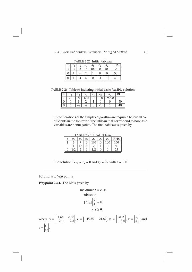
(c) We let a1 denote the artificial variable corresponding to the first(equality) constraint, and we let e2 and a2 denote the excess andartificial variables, respectively, that correspond to the second con-straint. Using M = 100, our objective becomes one of maximizingz = x1 + 5x2 + 6x3 − 100a1 − 100a2. The initial tableau is given by
To obtain an initial basic feasible solution, we pivot on each of thehighlighted entries in this tableau. The result is the following:
2.3. Excess and Artificial Variables: The Big M Method 41
TABLE 2.25: Initial tableauz x1 x2 x3 a1 e2 a2 RHS1 -1 -5 -6 100 0 100 0
0 1 4 2 1 0 0 50
0 1 -4 4 0 -1 1 40
TABLE 2.26: Tableau indicting initial basic feasible solution
z x1 x2 x3 a1 e2 a2 RHS1 -201 -5 -606 0 100 -90000 1 4 2 1 0 0 500 1 -4 4 0 -1 1 40
Three iterations of the simplex algorithm are required before all co-efficients in the top row of the tableau that correspond to nonbasicvariables are nonnegative. The final tableau is given by
TABLE 2.27: Final tableauz x1 x2 x3 a1 e2 a2 RHS1 2 7 0 103 0 100 1500 1 12 0 2 1 -1 600 1/2 2 1 1/2 0 0 25
The solution is x1 = x2 = 0 and x3 = 25, with z = 150.
Solutions to Waypoints
Waypoint 2.3.1. The LP is given by
maximize z = c · xsubject to
[A|I2]
[xs
]= b
x, s ≥ 0,
where A =
[1.64 2.67−2.11 −2.3
], c =
[−45.55 −21.87
], b =
[31.2−13.0
], x =
[x1
x2
], and
s =
[s1
s2
].

42 Chapter 2. The Simplex Algorithm
Waypoint 2.3.2. Let s1 denote the slack variable for the first constraint, andlet e2 and a2 denote the excess and artificial variables, respectively, for thesecond constraint. Using M = 100, our objective becomes one of minimizingz = 45.55x1 + 21.87x2 + 100a2. The initial tableau is as follows:
TABLE 2.28: Initial tableauz x1 x2 s1 e2 a2 RHS1 -45.55 -21.87 0 0 -100 00 1.64 2.67 1 0 0 31.2
0 2.11 2.3 0 -1 1 13.9
To obtain an initial basic feasible solution, we pivot on the highlighted entryin this tableau. The result is the following:
TABLE 2.29: Tableau indicting initial basic feasible solution
z x1 x2 s1 e2 a2 RHS1 165 208 0 -100 0 13900 1.64 2.67 1 0 0 13.20 2.11 2.3 0 -1 1 13.9
Two iteration of the simplex algorithm yield the final tableau:
TABLE 2.30: Final tableauz x1 x2 s1 e2 a2 RHS1 -26 0 0 -9.5 -90.5 132.170 -.81 0 1 1.16 -1.16 150 .918 1 0 -.435 .435 6.04
Thus x1 is nonbasic so that the total foraging time is minimized when x1 = 0grams of grass and x2 ≈ 6.04 grams of forb, in which case z ≈ 132.17 minutes
2.4. Duality 43
2.4 Duality
1. At each stage of the simplex algorithm, the decision variables in theprimal LP correspond to a basic feasible solutions. Values of the decisionvariables in the dual LP are recorded by the entries of the vector y. Onlyat the final iteration of the algorithm, do the dual variables satisfy bothyA ≥ c and y ≥ 0, i.e., only at the final iteration do the entries of yconstitute a basic feasible solution of the dual.
2. The given LP can be restated as
maximize z = 3x1 + 4x2
subject to
x1 ≤ 4
x1 + 3x2 ≤ 15
−x1 + 2x2 ≥ 5
x1 − x2 ≥ 9
x1 + x2 ≤ 6
−x1 − x2 ≤ −6
x1, x2 ≥ 0.
In matrix inequality form, this becomes
maximize z = c · xsubject to
Ax ≤ b
x ≥ 0,
where A =
1 01 31 −1−1 11 1−1 −1
, c =[3 4
], b =
415−596−6
, and x =
[x1
x2
].
The corresponding dual is given by
minimize w = y · bsubject to
yA ≥ c
y ≥ 0,

44 Chapter 2. The Simplex Algorithm
where y =[y1 y2 y3 y4 y5 y6
]. In expanded form this is identical
to
minimize w = 4y1 + 15y2 − 5y3 + 9y4 + 6(y5 − y6)
subject to
y1 + y2 + y3 − y4 + (y5 − y6) ≥ 3
3y2 − y3 + y4 + (y5 − y6)
y1, y2, y3, y4, y5, y6 ≥ 0.
Now define the new decision variable y = y5− y6, which is unrestrictedin sign due to the fact y5 and y6 are nonnegative. Since y5 and y6,together, correspond to the equality constraint in the primal LP, we seethat y is a dual variable unrestricted in sign that corresponds to anequality constraint in the primal.
3. The standard maximization LP can be written in matrix inequality formas
maximize z = ctx
subject to
Ax ≤ b
x ≥ 0,
where x belongs to Rn, c is a column vector in Rn, b belongs to Rm, andA is an m-by-n matrix.
The dual LP is then expressed as
minimize w = ytb
subject to
ytA ≥ ct
y ≥ 0,
where we have assumed the dual variable vector, y, is a column vectorin Rm. But, by transpose properties, this is equivalent to
maximize w = −bty
subject to
−Aty ≤ −c
y ≥ 0.
The preceding LP is a maximization problem, whose dual is given by

2.4. Duality 45
minimize z = xt(−c)
subject to
xt(−At) ≥ −bt
x ≥ 0.
Using transpose properties again, we may rewrite this final LP as
maximize z = ctx
subject to
Ax ≤ b
x ≥ 0,
which is the original LP.
4. (a) The original LP has four decision variables and three constraints.Thus, the dual LP has three decision variables and four constraints.
(b) The current primal solution is not optimal, as the nonbasic variable,s1, has a negative coefficient in the top row of the tableau. By theratio test, we conclude that s1 will replace x1 as a basic variableand that s1 = 4 in the updated basic feasible solution. Since thecoefficient of s1 in the top row is −2, the objective value in theprimal will increase to 28. By weak duality, we can conclude thatthe objective value in the solution of the dual LP is no less than 28.
5. The dual of the given LP is
minimize w = y1 − 2y2
subject to
y1 − y2 ≥ 2
−y1 + y2 ≥ 1
y1, y2 ≥ 0,
which is infeasible.
6. (a) The current tableau can also be expressed in partitioned matrixform as
z x y yb1 [�,�] [1, 0, 0] �
0 MA M Mb
Comparing this matrix to that given in the problem, we see that

46 Chapter 2. The Simplex Algorithm
M =
1/3 0 0−1/2 10
−1/3 0 1
. Thus,
b =M−1(Mb)
=
3 0 03/2 1 01 0 1
63
10
=
181216
,
and
A =M−1(MA)
=
3 0 03/2 1 01 0 1
−2/3 1
3 014/3 0
=
−2 32 3/24 1
.
Using A and b, we obtain the original LP:
maximize z = 2x1 + 3x2
subject to
−2x1 + 3x2 ≤ 18
2x1 +3
2x2 ≤ 12
4x1 + x2 ≤ 16
x1, x2 ≥ 0.
(b) The coefficients of x1 and x2 in the top row of the tableau are givenby
−c + yA = −[2, 3]+ [1, 0, 0]A
= [−4, 0]
The unknown objective value is
z = yb
= [1, 0, 0]
181216
= 18.
(c) The coefficient of x1 in the top row of the tableau is -4, so an ad-ditional iteration of the simplex algorithm is required. Performing

2.4. Duality 47
the ratio test, we see that x1 replaces s2 as a nonbasic variable. The
updated decision variables become x1 = 1 and x2 =20
3, with a
corresponding objective value of z = 22. The slack variable coeffi-cients in the top row of the tableau are s1 =
13 , s2 =
43 , and s3 = 0,
which indicates that the current solution is optimal. Therefore the
dual solution is given by y =
1/34/30
with objective value w = 22.
7. Since the given LP has two decision variables and four constraints, thecorresponding dual has four decision variables, y1, y2, y3, and y4 alongwith two constraints. In expanded form, it is given by
minimize z = 4y1 + 6y2 + 33y3 + 24y4
subject to
−y1 + 2y3 + 2y4 ≥ 1
y1 + y2 + 3y3 + y4 ≥ 5
y1, y2, y3, y4 ≥ 0.
To solve the dual LP using the simplex algorithm, we subtract excessvariables, e1 and e2, from the first and second constraints, respectively,and add artificial variables, a1 and a2. The Big M method with M = 1000yields an initial tableau given by
TABLE 2.31: Initial tableauw y1 y2 y3 y4 e1 a1 e2 a2 RHS1 -4 -6 -33 -24 0 -1000 0 -1000 00 -1 0 2 2 -1 1 0 0 10 1 1 3 1 0 0 -1 1 5
.
The final tableau is
TABLE 2.32: Final tableauw y1 y2 y3 y4 e1 a1 e2 a2 RHS1 -11/2 0 0 -3 -15/2 -1985/2 -6 -994 75/20 -1/2 0 1 1 -1/2 1/2 0 0 1/20 5/2 1 0 -2 3/2 -3/2 -1 1 7/2
.
The excess variable coefficients in the top row of this tableau are the

48 Chapter 2. The Simplex Algorithm
additive inverses of the decision variable values in the solution of the
primal. Hence, the optimal solution of the primal is given by x1 =15
2
and x2 = 6, with corresponding objective value z =75
2.
8. By the complementary slackness property, x0 is the optimal solution of
the LP provided we can find y0 =
y1
y2
y2
y4
in R4 such that
[y0A − c
]i [x0]i = 0 1 ≤ i ≤ 6
and
[y0] j [b − Ax0] j = 0 1 ≤ j ≤ 4.
We have
b − Ax0 =
00
61/70
,
so that in a dual solution it must be the case that y3 = 0. Furthermore,when y3 = 0,
y0A − c =
y1 + 7y2 + 7y4 − 52y1 − 5y2 + 8y4 − 14y1 + 2y2 − 3y4 − 13y1 + y2 + 5y4 − 4
4y1 + 2y2 + 2y4 − 16y1 + 3y2 + 4y4 − 2
.
By complementary slackness again, the first, third and fourth compo-nents of this vector must equal zero, whence we have a system of 3linear equations, whose solution is given by y1 =
103204 , y2 =
37204 , and
y3 =47
102 . If we define y0 =
103/20437/204
047/102
, then
w = y0b
=53
17= cx0
so that x0 is the optimal solution of the LP by Strong Duality.
2.4. Duality 49
9. Player 1’s optimal mixed strategy is given by the solution of the LP
maximize z subject to
Ax ≥ ze
et · x = 1
x ≥ 0,
and Player 2’s by the solution of the corresponding dual LP,
minimize w subject to
yA ≤ wet
y · e = 1
y ≥ 0.
Here e =
[11
]. The solution of the first LP is given by x0 =
[.7.3
]and the
solution of the second by x0 =
[.5.5
]. The corresponding objective value
for each LP is z = w = .5, thereby indicating that the game is biased inPlayer 1’s favor.
10. (a) Since A is an m-by-n matrix, b belongs toRm, and c is a row vectorinRn, the matrix M has m+n− 1 rows and m+n− 1 columns. Fur-
thermore, the transpose of a partitioned matrix,
[A BC D
], is given
by
[At Ct
Bt Dt
], which can be used to show Mt = −M.
(b) Define vecw0 =
yt
0x0
1
. Then w0 belongs to Rm+n+1 and has nonnega-
tive components since x0 and y0 are primal feasible and dual fea-sible vectors belonging to Rn and Rm, respectively. Furthermore,[w0]m+n+1 = 1 > 0. We have
Mw0 =
0m×m −A b
At 0m×n −ct
−bt c 0
yt
0x0
1
=
−Ax0 + bAtyt
0 − ct
−btyt0+ cx0
≥ 0

50 Chapter 2. The Simplex Algorithm
since the primal feasibility of x0 dictates Ax0 ≤ b, the dual feasi-bility of y0 and transpose properties imply Atyt
0≥ ct, and strong
duality forces btyt0= cx0.
(c) Letting κ, x0, and y0 be defined as in the hint, we have
0 ≤Mw0
=
0m×m −A b
At 0m×n −ct
−bt c 0
κyt
0κx0
κ
= κ
0m×m −A b
At 0m×n −ct
−bt c 0
[yt
0x0
]
= κ
−Ax0 + bAtyt
0 − ct
−btyt0+ cx0
Since κ > 0, we conclude that Ax0 ≤ b, Atyt0 ≥ ct, and cx0 ≥
btyt0. Transpose properties permit us to rewrite the second of these
matrix inequalities as y0A ≥ c. Thus x0 and y0 are primal feasibleand dual feasible, respectively. Moreover, the third inequality isidentical to cx0 ≥ y0b if we combine the facts btyt
0= y0b, each
of these two quantities is a scalar, and the transpose of a scalaris itself. But the Weak Duality Theorem also dictates cx0 ≤ y0b,which implies cx0 = y0b. From this result, we conclude x0 and y0
constitute the optimal solutions of the (4.1) and (4.3), respectively.
Solutions to Waypoints
Waypoint 2.4.1. In matrix inequality form, the given LP can be written as
maximize z = c · xsubject to
Ax ≤ b
x ≥ 0,
where vecx =
x1
x2
x3
, c = [3, 5, 2], A =
2 1 11 2 13 1 5−1 1 1
, and b =
= 2243
. The dual LP is
given by

2.4. Duality 51
minimize w = y · bsubject to
yA ≥ c
y ≥ 0,
where y =[y1 y2 y3 y4
]. In expanded form, this is equivalent to
minimize w = 2y1 + 2y2 + 4y3 + 3y4
subject to
2y1 + y2 + 3y3 − y4 ≥ 3
y1 + 2y2 + y3 + y4 ≥ 5
y1 + y2 + 5y3 + y4 ≥ 2
y1, y2, y3, y4 ≥ 0.
The original LP has its solution given by x0 =
2/32/30
with z0 =
16
3. The
solution of the dual LP is y0 =[1/3 7/3 0 0
]with w0 =
16
3.
Waypoint 2.4.2. 1. If Steve always chooses row one and Ed choosescolumns one, two, and three with respective probabilities, x1, x2, andx3, then Ed’s expected winnings are given by
f1(x1, x2, x3) =[1 0 0
]· A ·
x1
x2
x3
= x1 − x2 + 2x3,
which coincides with the first entry of the matrix-vector product, Ax.By similar reasoning,
f2(x1, x2, x3) =[0 1 0
]· A ·
x1
x2
x3
= 2x1 + 4x2 − x3
and
f3(x1, x2, x3) =[0 0 1
]· A ·
x1
x2
x3
= −2x1 + 2x3,
which equal the second and third entries of Ax, respectively.

52 Chapter 2. The Simplex Algorithm
2. If Ed always chooses column one and Steve chooses rows one, two, andthree with respective probabilities, y1, y2, and y3, then Steve’s expectedwinnings are given by
g1(y1, y2, y3) =[y1 y2 y3
]· A ·
100
= y1 + 2y2 − 2y3,
which coincides with the first entry of the product, yA. By similar rea-soning,
g2(y1, y2, y3) =[y1 y2 y3
]· A ·
010
= −y1 + 4y2
and
g3(y1, y2, y3) =[y1 y2 y3
]· A ·
001
= 2y1 − y2 + 2y3,
which equal the second and third entries of yA, respectively.
Waypoint 2.4.3. To assist in the formulation of the dual, we view the primalobjective, z, as the difference of two nonnegative decision variables, z1 andz2. Thus the primal LP can be expressed in matrix inequality form as
maximize[1 −1 01×3
]·
z1
z2
x
subject toe −e −A0 0 et
0 0 −et
·
z1
z2
x
≤
03×1
1−1
x ≥ 0 and z1, z2 ≥ 0.
If the dual LP has its vector of decision variables denoted by[y w1 w2
],
where y is a row vector inR3 with nonnegative components, and both w1 andw2 are nonnegative as well, then the dual is given by

2.4. Duality 53
minimize[y w1 w2
]·
03×1
1−1
subject to
[y w1 w2
]·
e −e −A0 0 et
0 0 ∗ −et
≥
[1 −1 01×3
]
y ≥ 01×3 and w1,w2 ≥ 0.
If we write w = w1 − w2, then this formulation to the dual simplifies to be
minimize w subject to
yA ≤ wet
y · e = 1
y ≥ 0.
54 Chapter 2. The Simplex Algorithm
2.5 Sufficient Conditions for Local and Global Optimal So-lutions
1. If f (x1, x2) = e−(x21+x2
2), then direct computations lead to the followingresults:
∇ f (x) =
[−2x1 f (x1, x2)−2x2 f (x1, x2)
]
and
H f (x) =
[(−2 + 4x2
1) f (x1, x2) 4x1x2 f (x1, x2)
4x1x2 f (x1, x2) (−2 + 4x22) f (x1, x2)
]
so that
∇ f (x0) ≈[−.2707−.2707
]
and
H f (x0) ≈[.2707 .5413.5413 .2702
].
Thus,
Q(x) = f (x0) + ∇ f (x0)t(x − x0) +1
2(x − x0)tH f (x0)(x − x0)
≈ 2.3007− 1.895x1 − 1.895x2 + .2707x21 + .2707x2
2 + 1.0827x1x2
The quadratic approximation together with f are graphed in Figure 2.1.
The solution is given by x =
[4.50
], with z = 27.
2. Calculations establish that Hessian of f is given by H f (x) = φ(x)A,
where φ(x) =1
(74 + .5x1 + x2 + x3)1/10and where
A =
.045 .09 .09.09 .19 .19.09 .19 .19
.

2.5. Sufficient Conditions for Local and Global Optimal Solutions 55
FIGURE 2.1: Plot of f with quadratic approximation
Observe that φ(x) > 0 for x in S and that A is positive semidefinite. (Itseigenvalues are .002, .423, and zero.)
Now suppose that x0 belongs to S and that λ0 is an eigenvalue of H f (x0)with corresponding eigenvector v. Then
λ0v = H f (x0)v
= φ(x0)Av,
implyingλ0
φ(x0)is an eigenvalue of A. Since φ(x0) > 0 and each eigen-
value of A is nonnegative, then λ0 must be nonnegative as well. Hence,H f (x0) is positive semidefinite, and f is convex.

56 Chapter 2. The Simplex Algorithm
3. (a) We have ∇ f (x) =
[2x1 + x2 − 1x1 + 4x2 − 4
], which yields the critical point,
x0 =
[01
]. Since H f (x) =
[2 11 4
]has positive eigenvalues, λ = 3±
√2,
we see that f is strictly convex onR2 so that x0 is a global minimum.
(b) We have∇ f (x) =
[2x1 − 10x2 + 4−10x1 + 14x2 − 8
], which yields the critical point,
x0 =
[−1/31/3
]. Since H f (x) =
[2 −10 −10 14
]has mixed-sign
eigenvalues, λ = 8 ± 2√
34, x0 is a saddle point.
(c) We have ∇ f (x) =
[−4x1 + 6x2 − 66x1 − 10x2 + 8
], which yields the critical point,
x0 =
[−3−1
]. Since H f (x) =
[−4 66 −10
]has negative eigenvalues,
λ = −7± 3√
5, we see that f is strictly concave on R2 so that x0 is aglobal maximum.
(d) We have ∇ f (x) =
[4x3
1− 24x2
1+ 48x1 − 32
8x2 − 4
], which yields a single
critical point at x0 =
[2
1/2
]. The Hessian simplifies to H f (x) =
[12(x1 − 2)2 0
0 8
]and has eigenvalues of 12(x1 − 2)2 and 8. Thus,
f is concave on R2 and x0 is a global maximum.
(e) We have ∇ f (x) =
[cos(x1) cos(x2)− sin(x1) sin(x2)
], which yields four critical
points: x0 = ±[π/2
0
]and x0 = ±
[0π/2
]. The Hessian is
H f (x) =
[− sin(x1) cos(x2) − cos(x1) sin(x2)− cos(x1) sin(x2) − sin(x1) cos(x2)
],
which yields a repeated eigenvalue, λ = −1, when x0 =
[π/2
0
], a
repeated eigenvalue λ = 1, when x0 =
[−π/2
0
], and eigenvalues
λ = ±1, when x0 =
[0±π/2
]. Thus, x0 =
[π/2
0
]is a local maximum,
x0 =
[−π/2
0
]is a local minimum, and x0 =
[0±π/2
]are saddle points.
(f) We have ∇ f (x) =
[2x1/(x2
1+ 1)
x2
], which yields a single critical point

2.5. Sufficient Conditions for Local and Global Optimal Solutions 57
at the origin. Since f is differentiable and nonnegative on R2, weconclude immediately that the origin is a global minimum. Inaddition,
H f (x) =
2(1−x1)2
(x21+1)2 0
01
.
The eigenvalues of this matrix are positive when −1 < x1 < 1. Thusf is is strictly convex its given domain.
(g) If f (x1, x2) = e−(
x21+x2
22
)
, then ∇ f (x) = f (x)
[x1
x2
]so that f has a sin-
gle critical point at the origin. The Hessian simplifies to H f (x) =
f (x)
x2
1− 1 x1x2
x1x2
x22− 1
, which has eigenvalues in terms of x given by
λ =
[− f (x)
(x21+ x2
2− 1) f (x)
]. Since f (x) > 0 and x2
1+ x2
2< 1, we have that
f is strictly concave on its given domain and the origin is a globalminimum.
4. We have ∇ f (x) = Ax − b, which is the zero vector precisely when x0 =
A−1b. The Hessian of f is simply A, so f is strictly convex (resp. strictlyconcave) on Rn when A is positive definite (resp. negative definite).Thus, x0 is the unique global minimum (resp. unique global maximum)of f .
When A =
[2 11 3
], b =
[−14
], and c = 6, x0 =
[−7/59/5
]. The eigenvalues of
A are λ =5 ±√
5
2, so x0 is the global minimum.
5. Write n =
n1
n2
n3
. Since n , 0, we lose no generality by assuming n3 , 0.
Solving ntx = d for x3 yields x3 as a function of x1 and x2:
f : R2 → R where f (x1, x2) = x21 + x2
2 +(d − n1x1 − n2x2)2
n23
.
The critical point of f is most easily computed using Maple and sim-
plifies to x0 =[n1d/‖n‖2, n1d/‖n‖2
]The eigenvalues of the Hessian are
λ1 = 2 and λ2 =2‖n‖2
n23
so that f is strictly convex and x0 is the global
minimum. The corresponding shortest distance is |d|‖n‖

58 Chapter 2. The Simplex Algorithm
For the plane x1+2x2+x3 = 1, n =
123
and d = 1. In this case, x0 =
1/141/7
3/14
with a corresponding distance of1√
14.
6. The gradient of f is ∇ f (x) =
[4x3
12x2
], which vanishes at the origin. Since f
is nonnegative and f (0) = 0, we see that x0 = 0 is the global minimum.
The Hessian of f at the origin is H f (0) =[0 0 0 2
], which is positive
semidefinite.
The function f (x1, x2) = −x41+x2
2has a saddle point at the origin because
f (x1, 0) = −x41
has a minimum at x1 = 0 and f (0, x2) = x22
has a maximum
at x2 = 0. The Hessian of f at the origin is again H f (0) =[0 0 0 2
].
7. The function f (x) = x41+ x4
2has a single critical point at x0 = 0, which
is a global minimum since f is nonnegative and f (0) = 0. The Hessianevaluated at x0 is the zero matrix, whose only eigenvalue is zero. Simi-larly, f (x) = −x4
1− x4
2 has a global maximum at x0 = 0, where its Hessianis also the zero matrix.
8. (a) Player 1’s optimal mixed strategy is the solution of
maximize = z
subject to
2x1 − 3x2 ≥ z
−x1 + 4x2 ≥ z
x1 + x2 = 1
x1, x2 ≥ 0,
which is given by x0 =
[7/103/10
], with corresponding objective value
z0 =1
2.
Player 2’s optimal mixed strategy is the solution of the correspond-ing dual LP,
minimize = w
subject to
2y1 − y2 ≤ w
−3y1 + 4y2 ≤ w
y1 + y1 = 1y1, y2 ≥ 0,
2.5. Sufficient Conditions for Local and Global Optimal Solutions 59
which is y0 =
[1/21/2
], with corresponding objective value w0 =
1
2.
(b) We have
f (x1, y1) =
[y1
1 − y1
]t
A
[x1
1 − x1
]
= 10x1y1 − 5x1 − 7y1 + 4,
whose gradient,∇ f (x1, y1) vanishes at x1 =7
10, y1 =
1
2. The Hessian
of f is a constant matrix having eigenvalues λ = ±10 so that this
critical point is a saddle point. The game value is f(
7
10,
1
2
)=
1
2.
(c) The only solution of f (x1, y1) = 12 is simply
(7
10,
1
2
).
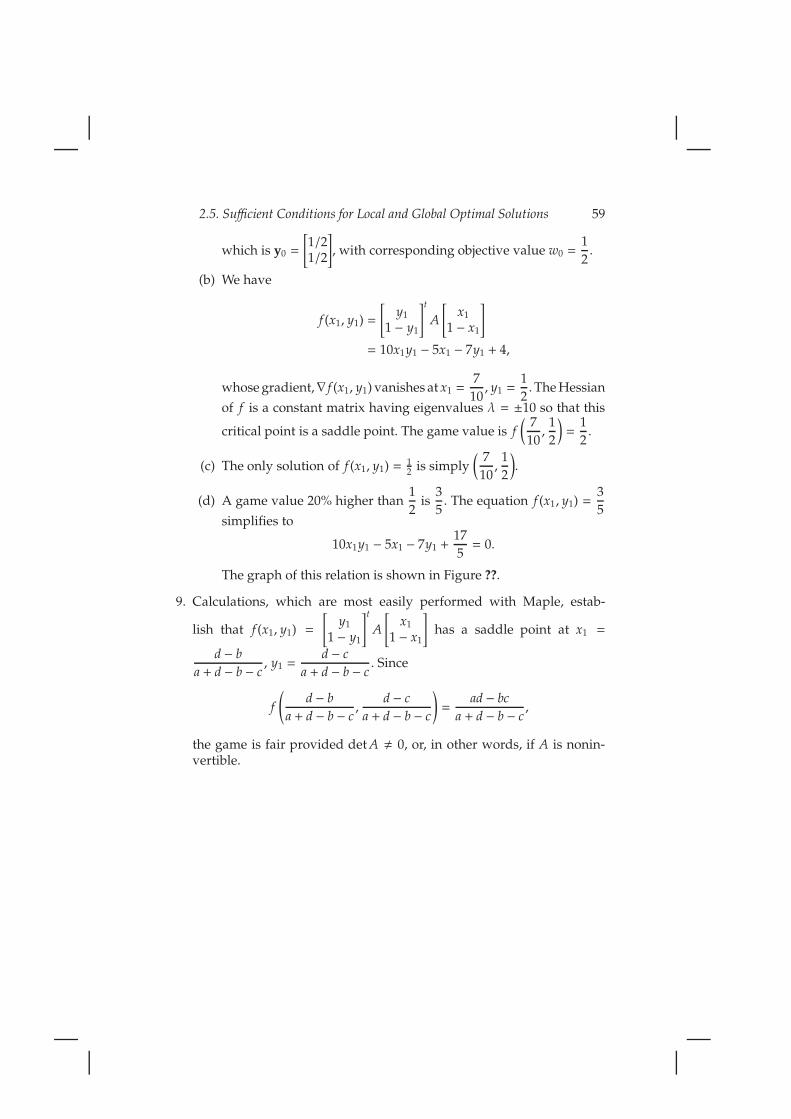
(d) A game value 20% higher than1
2is
3
5. The equation f (x1, y1) =
3
5simplifies to
10x1y1 − 5x1 − 7y1 +17
5= 0.
The graph of this relation is shown in Figure ??.
9. Calculations, which are most easily performed with Maple, estab-
lish that f (x1, y1) =
[y1
1 − y1
]t
A
[x1
1 − x1
]has a saddle point at x1 =
d − b
a + d − b − c, y1 =
d − c
a + d − b − c. Since
f
(d − b
a + d − b − c,
d − c
a + d − b − c
)=
ad − bc
a + d − b − c,
the game is fair provided det A , 0, or, in other words, if A is nonin-vertible.
60 Chapter 2. The Simplex Algorithm
x1
y1
FIGURE 2.2: The relation 10x1y1 − 5x1 − 7y1 +17
5= 0.

2.6. Quadratic Programming 61
2.6 Quadratic Programming
1. (a) The Hessian of f is
10 0 40 16 04 0 2
. If p =
12−1
, A =
[1 −1 11 2 1
], and
b =
[1−3
], then the problem is given as
minimize f (x) =1
2xtQx + ptx
subject to
Ax = b.
(b) The eigenvalues of Q are λ = 1 (repeated) and λ = 2, so Q ispositive definite and the problem is convex. Thus,
[µ0x0
]=
[0m×m A
At Q
]−1 [b−p
]
=
−44/965/9−1/3−4/3
0
.
The problem then has its solution given by x0 =
1/3−4/3
0
. The corre-
sponding objective value is f (1/3,−4/3) =106
9.
2. (a) The matrix Q is indefinite. However, the partitioned matrix,[0m×m A
At Q
]is still invertible so that
[µ0x0
]=
[0m×m A
At Q
]−1 [b−p
]
=
−259/311178/311−191/311−11/311−142/311
.
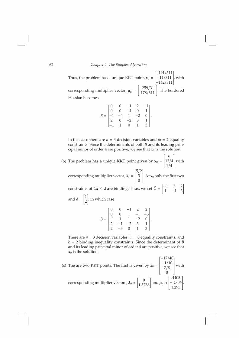
62 Chapter 2. The Simplex Algorithm
Thus, the problem has a unique KKT point, x0 =
−191/311−11/311−142/311
, with
corresponding multiplier vector, µ0 =
[−259/311178/311
]. The bordered
Hessian becomes
B =
0 0 −1 2 −10 0 −4 0 1−1 −4 1 −2 02 0 −2 3 1−1 1 0 1 3
.
In this case there are n = 3 decision variables and m = 2 equalityconstraints. Since the determinants of both B and its leading prin-cipal minor of order 4 are positive, we see that x0 is the solution.
(b) The problem has a unique KKT point given by x0 =
613/41/4
with
corresponding multiplier vector, λ0 =
5/230
. At x0 only the first two
constraints of Cx ≤ d are binding. Thus, we set C =
[−1 2 21 −1 3
]
and d =
[12
], in which case
B =
0 0 −1 2 20 0 1 −1 −3−1 1 1 −2 02 −1 −2 3 12 −3 0 1 3
.
There are n = 3 decision variables, m = 0 equality constraints, andk = 2 binding inequality constraints. Since the determinant of Band its leading principal minor of order 4 are positive, we see thatx0 is the solution.
(c) The are two KKT points. The first is given by x0 =
−17/40−1/10
7/80
with
corresponding multiplier vectors, λ0 ≈[
01.5788
]and µ0 ≈
.4405−.28061.295
.
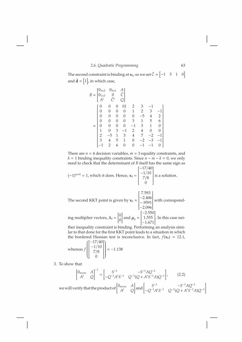
2.6. Quadratic Programming 63
The second constraint is binding at x0, so we set C =[−1 3 1 0
]
and d =[1], in which case,
B =
03×3 03×1 A01×3 0 CAt Ct Q
=
0 0 0 01 2 3 −10 0 0 0 1 2 3 −10 0 0 0 0 −5 4 20 0 0 0 3 1 5 60 0 0 0 −1 3 1 01 0 3 −1 2 4 0 02 −5 1 3 4 7 −2 −13 4 5 1 0 −2 −3 −1−1 2 6 0 0 −1 −1 0
There are n = 4 decision variables, m = 3 equality constraints, andk = 1 binding inequality constraints. Since n − m − k = 0, we onlyneed to check that the determinant of B itself has the same sign as
(−1)m+k = 1, which it does. Hence, x0 =
−17/40−1/10
7/80
is a solution.
The second KKT point is given by x0 ≈
7.593−2.406−.9591−2.096
with correspond-
ing multiplier vectors, λ0 =
[00
]and µ0 ≈
−2.5501.555−1.671
. In this case nei-
ther inequality constraint is binding. Performing an analysis simi-lar to that done for the first KKT point leads to a situation in whichthe bordered Hessian test is inconclusive. In fact, f (x0) ≈ 12.1,
whereas f
−17/40−1/10
7/80
≈ −1.138
3. To show that[0m×m A
At Q
]−1
=
[S−1 −S−1AQ−1
−Q−1AtS−1 Q−1(Q + AtS−1A)Q−1
], (2.2)
we will verify that the product of
[0m×m A
At Q
]and
[S−1 −S−1AQ−1
−Q−1AtS−1 Q−1(Q + AtS−1A)Q−1
]

64 Chapter 2. The Simplex Algorithm
is the (m+n)-by-(m+n) identity matrix. Viewing each of these two par-titioned matrices as being comprised of four blocks, we calculate fourdifferent products as follows:
Top left block of product:
0m×mS−1 − AQ−1AtS−1 = −AQ−1At(−AQ−1At)−1 (2.3)
= Im×m
Bottom left block of product:
AtS−1 −QQ−1AtS−1 = AtS−1 − AtS−1 (2.4)
= 0n×m (2.5)
Top right block of product:
−0m×mS−1AQ−1 + AQ−1(Q + AtS−1A
)Q−1 = AQ−1
(Q + AtS−1A
)Q−1
(2.6)
= AQ−1QQ−1 + AQ−1AtS−1AQ−1
= AQ−1 + AQ−1At(−AQ−1At
)−1AQ−1
(2.7)
= AQ−1 − Im×mAQ−1 (2.8)
= 0m×n (2.9)
Bottom right block of product:
−AtS−1AQ−1 +QQ−1(Q + AtS−1A
)Q−1 = −AtS−1AQ−1 +
(Q + AtS−1A
)Q−1
(2.10)
= −AtS−1AQ−1 + In×n + AtS−1AQ−1
= In×n. (2.11)
If we combine the results of (2.3)-(2.10), we see that
[0m×m A
At Q
] [S−1 −S−1AQ−1
−Q−1AtS−1 Q−1(Q + AtS−1A)Q−1
]=
[Im×m 0m×n
0n×m In×n
]
= Im+n.
4. We seek to maximize the probability an individual is heterozygous,namely 2x1x2 + 2x1x3 + 2x2x3, subject to the constraints that x1, x2, andx3 are nonnegative and sum to 1. Equivalently, we seek to minimizef (x) = −(2x1x2 + 2x1x3 + 2x2x3) subject to these same constraints. Since

2.6. Quadratic Programming 65
the Hessian of f is
0 −2 −2−2 0 −2−2 −2 0
, our quadratic programming problem,
in matrix form, is given by
minimize f (x) =1
2xtQx + ptx
subject to
Ax = b
Cx ≤ d,
where A =[1 1 1
], b = 1, C = −I3, and d =
000
.
The Lagrangian has a unique KKT point at x0 =
1/31/31/3
, with correspond-
ing multiplier vectors, λ0 =
000
andµ0 =
4
3, and corresponding objective
value f (x0) = −2
3. None of the three inequality constraints are binding,
so the bordered Hessian is simply
B
0 1 1 11 0 −2 −2 −21 −2 0 −21 −2 −2 0
In this case, n = 3, m = 1, and k = 0, so we only need to check that det(B)has the same sign as (−1)m+k = −1. Since det(B) = −12, x0 is optimal.
5. The solution of the bimatrix game is given by the solution of thequadratic programming problem
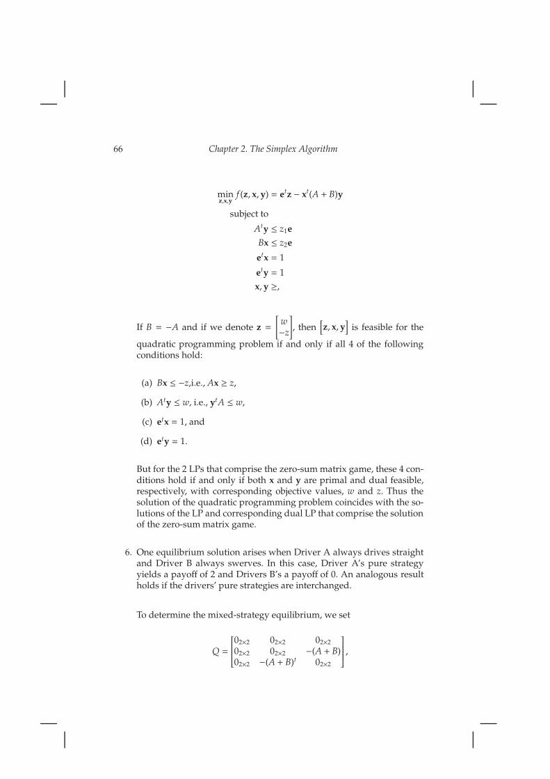
66 Chapter 2. The Simplex Algorithm
minz,x,y
f (z, x, y) = etz − xt(A + B)y
subject to
Aty ≤ z1e
Bx ≤ z2e
etx = 1
ety = 1
x, y ≥,
If B = −A and if we denote z =
[w−z
], then
[z, x, y
]is feasible for the
quadratic programming problem if and only if all 4 of the followingconditions hold:
(a) Bx ≤ −z,i.e., Ax ≥ z,
(b) Aty ≤ w, i.e., ytA ≤ w,
(c) etx = 1, and
(d) ety = 1.
But for the 2 LPs that comprise the zero-sum matrix game, these 4 con-ditions hold if and only if both x and y are primal and dual feasible,respectively, with corresponding objective values, w and z. Thus thesolution of the quadratic programming problem coincides with the so-lutions of the LP and corresponding dual LP that comprise the solutionof the zero-sum matrix game.
6. One equilibrium solution arises when Driver A always drives straightand Driver B always swerves. In this case, Driver A’s pure strategyyields a payoff of 2 and Drivers B’s a payoff of 0. An analogous resultholds if the drivers’ pure strategies are interchanged.
To determine the mixed-strategy equilibrium, we set
Q =
02×2 02×2 02×2
02×2 02×2 −(A + B)02×2 −(A + B)t 02×2
,

2.6. Quadratic Programming 67
p =
110000
, and
C =
M1 02×2 At
M2 B 02×2
02×2 −I2 02×2
02×2 02×2 −I2
,
where M1 =
[−1 0−1 0
], and M2 =
[0 −10 −1
]. We also set d = 08×1, E =
[0 0 1 1 0 00 0 0 0 1 1
], and b = e =
[11
].
Using Maple’s QPSolve command, we obtain a solution to the quadraticprogramming problem,
minimize f (w) =1
2wtQw + ptw
subject to
Ew = b
Cw ≤ d,
given by
w0 =
z0
x0
y0
=
1/21/21/21/21/21/2
.
Thus Driver A’s equilibrium strategy consists of x0 =
[1/21/2
], implying
that he chooses to drive straight or to swerve with equal probabilities
of1
2and that his payoff is z0,1 =
1
2. Driver B’s strategy and payoff are
exactly the same.
If we instead calculate the KKT points of the quadratic programmingproblem, we discover that there are exactly five:

68 Chapter 2. The Simplex Algorithm
(a) w0 =
201001
, with corresponding Lagrange multiplier vectors,λ0 =
10010110
and µ0 =
[20
], and with objective value, f (w0) = 0
(b) w0 =
020110
, with corresponding Lagrange multiplier vectors,λ0 =
01101001
and µ0 =
[02
], and with objective value, f (w0) = 0
(c) w0 =
1/21/21/21/21/21/2
, with corresponding Lagrange multiplier vectors, λ0 =
1/21/21/21/20000
and µ0 =
[1/21/2
], and with objective value, f (w0) = 0

2.6. Quadratic Programming 69
(d) w0 =
1/45/41/43/43/41/4
, with corresponding Lagrange multiplier vectors, λ0 =
01100000
and µ0 =
[01
], and with objective value, f (w0) =
1
4
(e) w0 =
5/41/43/41/41/43/4
, with corresponding Lagrange multiplier vectors, λ0 =
10010000
and µ0 =
[10
], and with objective value, f (w0) =
1
4
The first two KKT points correspond to the two pure strategy equilibriaand the third KKT to the mixed strategy equilibrium. That these are so-lutions of the original quadratic programming problem can be verifiedby use of the bordered Hessian test. By mere inspection of objective val-ues, we see that the latter two KKT points not solutions of the quadraticprogramming problem. In fact, the bordered Hessian test is inconclu-sive. Because these KKT points are not solutions of the problem, theydo not constitute Nash equilibria.
Solutions to Waypoints