institutional architectures and behavioral ecologies in the dynamics of financial markets
TRANSCRIPT
Journal of Mathematical Economics 41 (2005) 197–228
Institutional architectures and behavioral ecologiesin the dynamics of financial markets
Giulio Bottazzi∗, Giovanni Dosi, Igor RebescoS. Anna School of Advanced Studies, P.za Martiri della Liberta 33, Pisa, Italy
Received 8 November 2002; received in revised form 11 July 2003; accepted 16 February 2004Available online 2 July 2004
Abstract
The paper examines the properties of financial market dynamics, under different trading proto-cols. We start with an empirical analysis of the statistical properties of daily data from the world’smajor Stock Exchanges, comparing the behavior of different market phases characterized by dif-ferent trading protocols. The evidence lends support to the importance of investigating the outcomeof alternative market mechanisms. Motivated by this finding, we present an agent-based modelallowing the consistent treatment of agents’ behavior under three different trading set-ups, namelya Walrasian auction, a batch auction and an ‘order-book’ mechanism. The results highlight theimportance of the institutional setting in shaping the dynamics of the market but also suggest thatthe latter can become the outcome of a complicated interaction between the trading protocol andthe ecology of traders behaviors. In particular, we show that market architectures bear a centralinfluence upon the time series properties of market dynamics. Conversely, the revealed allocativeefficiency of different market settings is strongly influenced by the trading behavior of agents.© 2003 Elsevier B.V. All rights reserved.
Keywords:Financial market; Trading protocol; Market; Architecture
1. Introduction
In this work we explore the impact of different institutional structures governing financialmarket interactions upon market dynamics. Motivated also by some suggestive comparativeevidence drawn from the world’s largest Stock Exchanges, we compare the propertiesof three alternative market models, namely (i) Walrasian auctions (ii) batch auction-typemarkets and (iii) ‘order-book’-type markets.
∗ Corresponding author. Tel.:+39 050 883343; fax:+39 050 883344.E-mail address:[email protected] (G. Bottazzi).
0304-4068/$ – see front matter © 2003 Elsevier B.V. All rights reserved.doi:10.1016/j.jmateco.2004.02.006
198 G. Bottazzi et al. / Journal of Mathematical Economics 41 (2005) 197–228
The roots of the investigation ramify well beyond the confines of financial markets. Theyconcern indeed one of the most controversial questions which the economic discipline hasfaced since its origins, that is: What determines the relatively orderly aggregate properties –if any – and the degrees of efficiency of market exchanges? Are they mainly due to what goeson in the agents’ minds, or, conversely, are they primarily the outcome of some organizingprocesses which market mechanisms themselves impose? And, if market mechanisms matterat all, how do they fare in terms of comparative efficiency, however defined? Ultimately,one may think of two basic interpretations (with many combinations thereof).
A first one emphasizes the purported equilibrating features stemming from the fine un-derstanding that agents supposedly hold of both of their environment (possibly includingthe strategies of other agents) and of the means to pursue their interests. Obviously, “rationalexpectations” are the extreme version, but – in much milder forms – the emphasis on theequilibrating (or disequilibrating) role of agents’ beliefs and behavioral rules dates back atleast to Adam Smith’sTheory of Moral Sentiments.
A second, nearly opposite, view focuses upon the properties of particular distributionsof budget-constrained behaviors over heterogeneous, possibly ‘bounded rational’, popu-lations. A prominent example is Gode and Sunder’s analysis of markets populated by‘zero-intelligence’ agents (Gode and Sunder, 1993, see however also the critical remarks inCliff and Bruten, 1997).
Come as it may, institutions governing thephysics of exchanges– including centralizedversus decentralized trading mechanisms, the frequency of trading, the rules for price for-mation and those prescribing who is trading with whom and when – are central to this latterinterpretation, but are also likely to be important parts of the former ones, except for theirsimplest versions. After all, market institutions also shape the information agent access, theprocesses of competition and selection, the mechanisms of aggregation and price formation,etc.
However, surprising as it sounds, not much work has gone into the study of the aggregateimplications of different architectures of both financial and real markets1. As LeBaron endshis survey of agent-based models of financial markets, one of the major open issues aheadconcerns the study of the properties of different trading set-ups (LeBaron, 2000, p. 698).This is also the point of departure of this work which tries to identify some distinctiveproperties of diverse market mechanisms.
More precisely, one begins to address two challenging questions, namely,
(i) what happens to market dynamics if one changes market interaction mechanisms, whileholding constant individual characteristics (including the distribution of cognitive andbehavioral patterns), and, conversely,
(ii) holding constant institutional set-ups governing information diffusion and interactionpatterns, what happens as one varies the “ecology” of behavioral types of agents?
1 Among the remarkable exceptions one finds the studies by Alan Kirman and collaborators: see for example,Kirman and Vignes (1991)on the fish market. Concerning financial markets, ‘microstructure’ studies (seeGoodhartet al., 1996) certainly represent a major step in the right direction, although one still falls short of any explicitaccount of the dynamics of exchange.
G. Bottazzi et al. / Journal of Mathematical Economics 41 (2005) 197–228 199
We address these questions making use of an agent-based simulation model2 describingheterogeneous populations of boundedly rational, budget-constrained agents trading anasset whose price is endogenously determined by market exchanges. Agents are endowedwith an “adaptive” rationality on which they ground their expectations about the future priceof the asset. In our model, different types of agents come to different expectations even inpresence of an identical information. In turn, these expectations shape their behavior inthe market. For the time being, we freeze all learning and all selection processes and wefocus on the comparative properties of diverse institutional architectures, i.e. diverse tradingmechanisms, nesting different populations of traders.
The spirit of the model which follows is to a large extent akin that inspiring alreadyexisting computer-simulated “artificial financial markets”, such as those byArthur et al.(1997), Beltratti and Margarita (1992), Brock and Hommes (1998), Chiaromonte et al.(1998), Farmer (2002), Hens et al. (2002), Lux and Marchesi (1999), Marengo and Tordjman(1996)andYang (2000)(see the review inLeBaron, 2000).
Obvious common points of departure are (i) the acknowledgment of the limitations ofmodels of market dynamics centered upon the behavior of a mythical representative agentendowed with unbiased forward-looking expectations and, conversely, (ii) the challenge offounding the theory on an explicit account of heterogeneous interactive agents.
Within such a common perspective, however, distinct families of models significantlydiffer in the ways they model both the agents’ behavioral repertoires and the mechanismsof interaction.
In particular, regarding trading protocols, one finds three basic modeling styles and varia-tions thereof. A first one generates temporary equilibrium prices making use of a Walrasianmechanism (see for example,Brock and Hommes, 1998). Conversely, a secondgenresum-marizes collective interactions into some “law” governing price responses to excess demandsentailing price dynamics in persistent disequilibrium cf.Farmer (2002). Finally, a third fam-ily of models attempts to account for explicit trading mechanisms (this family includesLuxand Marchesi, 1999; Chiaromonte and Dosi, 1998among others). Remarkably, however,even those models taking the latter route have hardly addressed systematic comparisons ofthe properties of different mechanisms. In fact, in the analysis of the results of the differentagent-based models of speculative trading, one finds it hard to disentangle the effects ofsheer market organization from the impact of agents behaviors. To what extent are suchresults dependent on the assumed ecology of beliefs and to what extent are they due to thechosen trading protocols? These questions are the central tasks of the present work.
In Section 2we present some novel evidence on the properties of daily time series un-der the two alternative market protocols which distinguish the opening and trading phasesof major Stock Exchanges. While a few statistical ‘stylized facts’ hold across country andmarket regimes, finer properties are seemingly influenced by the latter. InSection 3we intro-duce our model, describing the implementation of the different trading protocols and of the
2 The software used for this work is part of the YAFiMM package, which is publicly available athttp://www.sssup.it/ bottazzi. Early investigations of the model have been conducted on ‘The Financial Toy Room’(FTR), a general purpose simulation environment originally developed by Francesca Chiaromonte and collabora-tors at the International Institute of Applied System Analysis (IIASA), Laxenburg, Austria: cf.Chiaromonte andDosi (1998). FTR is now available at the sitehttp://ftrsim.sssup.it.
200 G. Bottazzi et al. / Journal of Mathematical Economics 41 (2005) 197–228
behavior of the different agents. InSection 4we undertake a partial analytical investigationof the model. This analysis represent a useful benchmark for the numerical investigationsperformed inSection 5. The simulation results robustly support the importance of spe-cific institutional arrangements, and, together, they hint at a thread of interactions betweenmarket institutions and behavioral ecologies. Finally, inSection 6we undertake a compari-son between “artificial” and empirically observed market set-ups, highlighting encouragingqualitative analogies.
2. Generic stylized facts and institution-dependent phenomena
A good deal of current research on the statistical properties of financial time-series hasgone, for sound reasons of scientific priority, into the identification of robust, generic prop-erties which appear to hold across markets and temporal windows of observation. As wellknown, such stylized facts include fat-tailed distributions of returns; ARCH effects; auto-correlation of volumes and cross-correlation volumes/volatility (for detailed discussions,cf. Brock and de Lima, 1995; Dacorogna et al., 2001; Guillaume et al., 1997; Levy et al.,2000). Together, quite a few studies, broadly in the ‘microstructure perspective’, have beenalso devoted to the degrees to which particular market organizations contribute to parame-terize the foregoing generic properties and/or yield further institution-specific phenomena(cf. among othersAmihud and Mendelson, 1987; Biais et al., 1999; Madhavan, 1992; Stolland Whaley, 1990, and the survey inCalamia, 1999).
One way of tackling the latter topics, which we share here, is by exploiting the fact thatmost Stock Exchanges daily undergo the transition between two diverse sets of marketprotocols. A first opening section is typically organized as a periodic batch auction inwhich orders are collected during a call period to form demand and supply schedules thatare crossed to determine the unique equilibrium price (corresponding to the maximumexecutable volume) at which all transactions occur. This is followed by a trading sectioncharacterized by continuous double auctions in which each agent can post bid and askprices. In turn such continuous auctions may involve (i) a special category of agents – themarket makers –surrogating the auctioneer and making public either firm bid and ask prices(under the “quote-driven” system) or buy/sell intentions (under the “order-driven” system)and, (ii) an order book in which limit orders are stored waiting to be bit or taken by marketones. The trading phase terminates with a closing section yielding the fixing, i.e. the closingprice computed as the average of transaction prices, weighted by respective quantities, overthe last period of the trading section.
Given the significant difference in the architectures of exchanges between the openingand trading phases, their comparison might reveal precious albeit circumstantial informationon their comparative properties.
So, for example,Amihud and Mendelson (1987)andStoll and Whaley (1990)comparethe open-to-open and close-to-close daily series on the NYSE highlighting higher volatilityand negative autocorrelation of returns in the former.
Expanding on such a line of inquiry, here we compare the open-to-open and close-to-closedaily series for “blue-chips” over periods of at least 1000 trading days taken, subject to dataavailability, within the window 1 January 1997 to 14 April 2002 for the Stock Exchanges of
G. Bottazzi et al. / Journal of Mathematical Economics 41 (2005) 197–228 201
CAC DAX MIB DJIA IBEX LSE TPX TSE
-0.1
-0.05
0
0.05
0.1
0.15
open: 1st col.
close: 2nd col.
Autocorrelation of returns
Markets
corr
elat
ion
coef
ficie
nt
confidence intervals
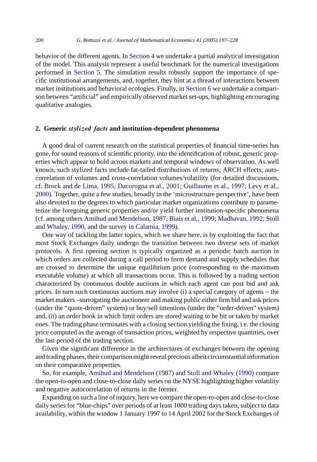
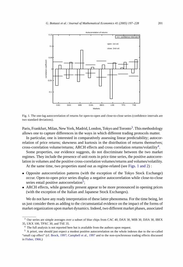
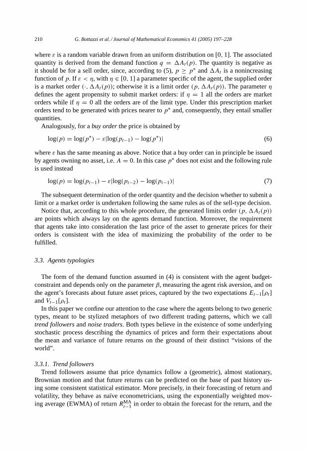
Fig. 1. The one-lag autocorrelation of returns for open-to-open and close-to-close series (confidence intervals aretwo standard deviations).
Paris, Frankfurt, Milan, New York, Madrid, London, Tokyo and Toronto3. This methodologyallows one to capture differences in the ways in which different trading protocols matter.
In particular, one is interested in comparatively assessing linear predictability; autocor-relation of price returns; skewness and kurtosis in the distribution of returns themselves;cross-correlation volume/returns; ARCH effects and cross correlation returns/volatility4.
Some properties, our evidence suggests, do not discriminate between the two marketregimes. They include the presence of unit roots in price time series, the positive autocorre-lation in volumes and the positive cross-correlation volumes/returns and volumes/volatility.
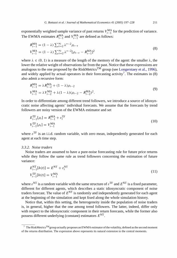
At the same time, two properties stand out as regime-related (seeFigs. 1 and 2) :
• Opposite autocorrelation patterns (with the exception of the Tokyo Stock Exchange)occur. Open-to-open price series display a negative autocorrelation while close-to-closeseries entail positive autocorrelation5;
• ARCH effects, while generally present appear to be more pronounced in opening prices(with the exception of the Italian and Japanese Stock Exchanges).
We do not have any ready interpretation of these latter phenomena. For the time being, letus just consider them as adding to the circumstantial evidence on the impact of the forms ofmarket organization upon market dynamics. Indeed, two different market phases, associated
3 Our series are simple averages over a subset of blue chips from CAC 40, DAX 30, MIB 30, DJIA 30, IBEX35, UKX 100, TPXC 30, and TSE 35.
4 The full analysis is not reported here but is available from the authors upon request.5 A priori, one should just expect a modest positive autocorrelation on the whole indexes due to the so-called
“small cap effect” (cf.Brock, 1997; Campbell et al., 1997and to the non-synchronous trading effects discussedin Fisher, 1966.)

202 G. Bottazzi et al. / Journal of Mathematical Economics 41 (2005) 197–228
CAC DAX MIB DJIA IBEX LSE TPX TSE 0
20
40
60
80
100
120ARCH test
markets
Sta
tistic
s
1st bar: open
2nd bar: close
critical value 5%
Fig. 2. Testing for ARCH effects for open-to-open and close-to-close returns.
to different trading protocols and intertwined in an appropriate order, are involved in thedetermination of the open-to-open and close-to-close returns. In the open-to-open case, acontinuous trading phase follows the opening batch auction, while the opposite applies tothe close-to-close case.
In this respect, it is equally interesting to independently analyze the dynamics overtime of each market phase, considered as a proxy of a distinct trading protocol. Theclose-to-next-open returns can provide evidence on the behavior of the opening phase batchauction, while the analysis of the open-to-close returns witnesses for the dynamics generatedby the continuous trading phase.
Some problems do however arise in the latter case with time series of returns because thetrading phase is often a complex mixing of continuous trading sessions and market makerintervention (sometimes interrupted by intra-day batch auctions). They involve differenttrading protocols and it is impossible to disentangle their effects in the open-to-close seriesof returns. In order to overcome this drawback we have singled out a market segment whosecontinuous trading phase is characterized by a pure ‘order book’ protocol, namely the StockExchange Electronic Trading Services (SETS) of the London Stock Exchange (LSE) ofwhich we have analyzed daily data for 73 equities over the time window 1 January 1997to 14 April 2002. InTable 1we report some basic statistics computed on their unweighted
Table 1Statistics from SETS of LSE. The annual volatility is computed multiplying the daily standard deviation by
√250
Returns Skewness Kurtosis Absolute deviation Annual volatility
Close-to-next-open −2.51 37.7 0.0034 0.084Open-to-close 0.46 8.4 0.006 0.13
G. Bottazzi et al. / Journal of Mathematical Economics 41 (2005) 197–228 203
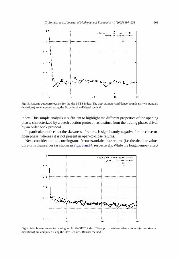
Fig. 3. Returns autocorrelogram for the the SETS index. The approximate confidence bounds (at two standarddeviations) are computed using the Box–Jenkins–Reinsel method.
index. This simple analysis is sufficient to highlight the different properties of the openingphase, characterized by a batch auction protocol, as distinct from the trading phase, drivenby an order book protocol.
In particular, notice that the skewness of returns is significantly negative for the close-to-open phase, whereas it is not present in open-to-close returns.
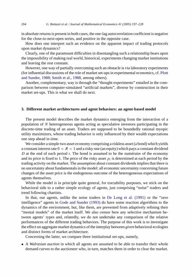
Next, consider the autocorrelogram of returns and absolute returns (i.e. the absolute valuesof returns themselves) as shown inFigs. 3 and 4, respectively. While the long memory effect
Fig. 4. Absolute returns autocorrelogram for the SETS index. The approximate confidence bounds (at two standarddeviations) are computed using the Box–Jenkins–Reinsel method.
204 G. Bottazzi et al. / Journal of Mathematical Economics 41 (2005) 197–228
in absolute returns is present in both cases, the one-lag autocorrelation coefficient is negativefor the close-to-next-open series, and positive in the opposite case.
How does one interpret such an evidence on the apparent impact of trading protocolsupon market dynamics?
Clearly, one of the paramount difficulties in disentangling such a relationship bears uponthe impossibility of making real world, historical, experiments changing market institutionsand leaving the rest constant.
However, one way of partially overcoming such an obstacle is via laboratory experiments(for influential discussions of the role of market set-ups in experimental economics, cf.Plottand Sunder, 1988; Smith et al., 1988, among others).
Another, complementary, way is through the “thought experiments” entailed in the com-parison between computer-simulated “artificial markets”, diverse by construction in theirmarket set-ups. This is what we shall do next.
3. Different market architectures and agent behaviors: an agent-based model
The present model describes the market dynamics emerging from the interaction of apopulation ofN heterogeneous agents acting as speculative investors participating in thediscrete-time trading of an asset. Traders are supposed to be boundedly rational myopicutility maximizers, whose trading behavior is only influenced by their wealth expectationsone step ahead in time.
We consider a simple two asset economy comprising a riskless asset (a bond) which yieldsa constant interest rate 0< R < 1 and a risky one (an equity) which pays a constant dividendD at the end of each periodt. The bond is assumed to be the numéraire of the economyand its price is fixed to 1. The price of the risky assetpt is determined at each period by thetrading activity on the market. The assumption about constant dividends implies that there isno uncertainty about fundamentals in the model: all economic uncertainty concerning futurechanges of the asset price is the endogenous outcome of the heterogeneous expectations ofagents themselves.
While the model is in principle quite general, for tractability purposes, we stick on thebehavioral side to a rather simple ecology of agents, just comprising “noise” traders andtrend following chartists.
In that, our agents, unlike the noise traders inDe Long et al. (1991)or the “zerointelligence” agents inGode and Sunder (1993)do have some reaction algorithms to thedynamics of the environment, but, like them, are prevented from adaptively refining their“mental models” of the market itself. We also censor here any selective mechanism be-tween agents’ types and, relatedly, we do not undertake any comparison of the relativeperformances of the different trading behaviors. The purpose of this work is to investigatethe effect on aggregate market dynamics of the interplay betweengivenbehavioral ecologiesand distinct forms of market architecture.
Concerning the latter, we compare three institutional set-ups, namely,
• A Walrasian auctionin which all agents are assumed to be able to transfer their wholedemand curves to the auctioneer who, in turn, matches them in order to clear the market.
G. Bottazzi et al. / Journal of Mathematical Economics 41 (2005) 197–228 205
• A batch auctionin which each agent can simultaneously post abuyor asell order, bothof limit andmarkettypes. Demand and supply schedules are then derived and crossed inorder to determine the equilibrium price at which all agents exchange.
• An order bookin which agents can post both market and limit orders that are matchedfollowing a price priority.
The next Section describes the implementation of the foregoing protocols in our model. Thedescription of the different protocols will also clarify the kind of requirements they imposeon the description of the agents behavior, that will be illustrated inSection 3.2.
3.1. The trading protocols
In each round of theWalrasian auctioneach agenti ∈ {1, . . . , N} is supposed to providethe auctioneer with its complete individual demand curveAi,t(p), i.e. the amount of theassetA that it is willing to buy (A > 0) or sell (A < 0) for each possible pricep. Theauctioneer then computes the aggregate excess demandAt(p) = ∑
i Ai,t(p) and fixesthe asset pricept at the value that clears the market:At(pt) = 0. Notice that, in general,the individual demand functions are time-dependent as agents react to changing “marketconditions”. However, as long as individual demand curves are well-behaved decreasingfunctions, the existence and uniqueness ofpt is guaranteed.
This stylized exchange protocol provides a price fixing mechanism that forces the marketto equilibrium at each iteration. Such a feature makes it an excellent analytical benchmark.At the same time, since the amount of information that the agents must provide to theauctioneer is infinite, encompassing all the possible desired positions for all the possibleprices, this can hardly represent a sound approximation of any real trading mechanismwherein processing of (finite) information always entails a non-zero cost, no matter howsmall.
The other two trading protocols that we shall analyse are indeed based on the processingof a finite amount of information.
In the batch auction, at each round, each agent provides a (finite) number of “orders”that can be considered as statements concerning the conditions for its participation to themarket. The following two basic instances of an order are analyzed:
Limit ordersrepresented as ordered couples(p, q) of a pricep > 0 and a quantityq.For “buy limit orders” (q > 0), the pricep stands for the maximum price at which theorder issuer is willing to buy the quantityq of the asset. For “sell limit orders” (q < 0),p is the minimum price at which the order issuer wants to sell a quantityq.
Market orders(·, q) express only a quantity that should be sold (“sell market orders”),if q < 0, or bought (“buy market orders”), ifq > 0 at the best available price on themarket (the lowest for buy orders and the highest for sell orders).
Once all the limit and market orders are collected, the auctioneer uses them to builddemand and supply schedules, computing the total amount of the asset demanded andoffered at a given notional price. Within this procedure, the market orders are “priced” atthe price that is more likely to guarantee their fulfillment among the prices of the limitorders of the same side, that is the largest price for buy orders and the smallest for sell
206 G. Bottazzi et al. / Journal of Mathematical Economics 41 (2005) 197–228
M
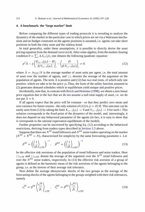
Qnty
PriceP'P DS
S'
S''D'
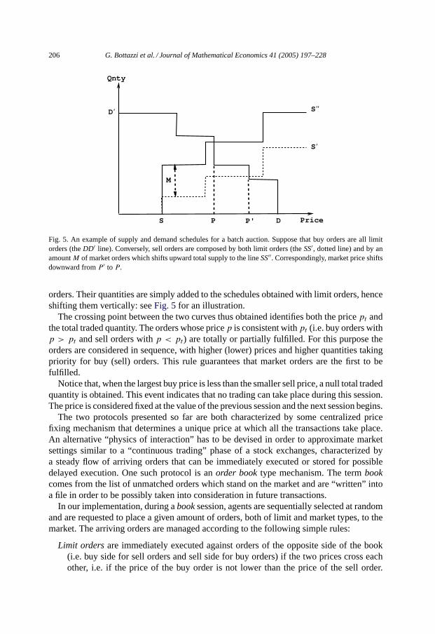
Fig. 5. An example of supply and demand schedules for a batch auction. Suppose that buy orders are all limitorders (theDD′ line). Conversely, sell orders are composed by both limit orders (theSS′, dotted line) and by anamountM of market orders which shifts upward total supply to the lineSS′′. Correspondingly, market price shiftsdownward fromP ′ to P .
orders. Their quantities are simply added to the schedules obtained with limit orders, henceshifting them vertically: seeFig. 5for an illustration.
The crossing point between the two curves thus obtained identifies both the pricept andthe total traded quantity. The orders whose pricep is consistent withpt (i.e. buy orders withp > pt and sell orders withp < pt) are totally or partially fulfilled. For this purpose theorders are considered in sequence, with higher (lower) prices and higher quantities takingpriority for buy (sell) orders. This rule guarantees that market orders are the first to befulfilled.
Notice that, when the largest buy price is less than the smaller sell price, a null total tradedquantity is obtained. This event indicates that no trading can take place during this session.The price is considered fixed at the value of the previous session and the next session begins.
The two protocols presented so far are both characterized by some centralized pricefixing mechanism that determines a unique price at which all the transactions take place.An alternative “physics of interaction” has to be devised in order to approximate marketsettings similar to a “continuous trading” phase of a stock exchanges, characterized bya steady flow of arriving orders that can be immediately executed or stored for possibledelayed execution. One such protocol is anorder booktype mechanism. The termbookcomes from the list of unmatched orders which stand on the market and are “written” intoa file in order to be possibly taken into consideration in future transactions.
In our implementation, during abooksession, agents are sequentially selected at randomand are requested to place a given amount of orders, both of limit and market types, to themarket. The arriving orders are managed according to the following simple rules:
Limit ordersare immediately executed against orders of the opposite side of the book(i.e. buy side for sell orders and sell side for buy orders) if the two prices cross eachother, i.e. if the price of the buy order is not lower than the price of the sell order.
G. Bottazzi et al. / Journal of Mathematical Economics 41 (2005) 197–228 207
The execution price is the one associated with the order already in the book andthe quantity is the smaller between the two orders. If the first matching does notcompletely fulfill the arriving order, this operation is continued until either: (i) nosuitable order remains on the opposite side, or, (ii) the arriving order is completelyfulfilled.
In the cases in which either there is no order on the opposite side of the book, orthere is no crossing, or the order is not completely fulfilled, the order is stored in the“book” on the basis of price/quantity/time priorities. Higher (lower) priced bids (asks)have priority over lower (higher) ones. Among the orders with the same posted price(bid or ask) the ones with higher posted quantity are executed first. Among the orderswith the same posted price and quantity, older ones have priority.
Market ordersare treated analogously, after assigning them a price equal to the best orderon the opposite side. Therefore a market buy order will immediately match the lowestask price and a sell market order will “take” right off the highest bid price. If thereare no orders on the opposite sides, a market order is stored on the book assigning ita reference price, i.e. it becomes a limit order with a limit price equal to thereferenceprice.
Thereference priceis equal to the price of the last transaction or to the fixing price of thelast trading session if no transactions have taken place yet. The fixing price of the sessionis the last reference price of the session.
3.2. The Agents
The implementation of the foregoing trading protocols involves the basic requirement forthe agent that it should be able both to provide the auctioneer with a well-behaved demandfunction and, alternatively, to provide “the market” with limit/market orders. However, inorder to compare market dynamics under different protocols, it is mandatory to model asmuch as possible agents behaviors as governed by the same rules and as shaped by the samekind of information when the different trading protocols are considered. Ultimately, thismeans that the way in which agents generate the orders to be posted in the batch auctionand book protocols should be consistent with the demand function they transmit to theauctioneer in the Walrasian auction.
Let us thus turn to the description of how agents, in our model, build their individualdemand functions and of the mechanism with which they generate, consistently with suchdemand functions, the orders they transmit to the market.
3.2.1. The demand functionAt the beginning of each trading session, each agent constructs its individual demand
function and determines the amount of wealth it would like to invest in the risky asset forany possible value of the notional transaction pricep. The residual wealth is invested in theriskless asset.
For simplicity, in this Section we drop the agent index from all variables. The followingprocedure for the determination of individual demand functions is understood to apply toevery agenti ∈ {1, . . . , N}.
208 G. Bottazzi et al. / Journal of Mathematical Economics 41 (2005) 197–228
Let Wt be the wealth of the agent at timet and letBt andAt be the amount of bondand stock present in its portfolio, respectively. Denote withxt = Atpt/Wt the share of theagent’s wealth invested in the risky asset. Then the wealth of the agent at periodt + 1 as afunction of the stock returnρt = pt+1/pt − 1 reads:
Wt+1 = Wt(1 + R) + xtWt
(ρt − R + D
pt
)(1)
The future value of the portfolio obviously depends on the future price of the stock.Let us suppose that the agent possesses some forecasting abilities concerning the futureprice returnρt , which are used to formulate expectations on its own future wealth and,consistently with these expectations, to maximize its expected utilityU. We represent forconvenience the expected utility of the agent by the simplest function of the expected returnand variance (Brock and Hommes, 1998; Hommes, 2001; Kirman and Teyssie‘re, 2002)
Ut = Et−1Wt+1 − 12βVt−1Wt+1 (2)
whereEt−1[·] stands for the expected mean andVt−1[·] stands for the expected varianceof the distribution of returnρt computed at the beginning of timet, i.e. conditional on theinformation available at timet − 1, andβ is the “risk-aversion” parameter6.
Using the expression forWt+1 in (1) one obtains
Et−1[Wt+1] = xWt
(Et−1[ρt ] − R + D
pt
)+ Wt(1 + R)
Vt−1[Wt+1] = x2W2t Vt−1ρt
(3)
The portfolio composition chosen by the agent is the one that maximizes the expressionin (2). From the first order condition dUt/dx = 0 and using (3) one immediately obtains
At(pt) = −At−1 + Et−1[ρt ] − R + D/pt
β Vt−1[ρt ] pt
(4)
whereAt−1 stands for the quantity of risky asset in the agents’ portfolio at the end of theprevious trading session andAt = At −At−1 is the quantity of stock the agent is willingto trade (i.e. to buy if it is positive or to sell if it is negative) at timet conditional on thestock pricept .
The individual demand function is inversely proportional to the risk aversion parameterβ. This parameter set the “scale” of the agent’s position on the market and, as we will seein the next section, basically defines the impact of the agent on the trading activity. Whenβ � 1 even a relatively low uncertainty on the future asset price is sufficient to stronglydecrease its attractiveness for the agent; conversely forβ 1 the opposite holds.
Notice that the demand function in (4) is obtained from a Constant Absolute Risk Aver-sion (CARA) utility function and does not explicitly contain the wealth of the agent: thedesired amount of asset depends on the agent’s forecast on future asset performances, butis independent from the agent’s actual wealth.
6 The same expression can be obtained from EUT with a negative exponential utility functionU(W) =−exp(−βW) under the hypothesis of normally distributed returns.
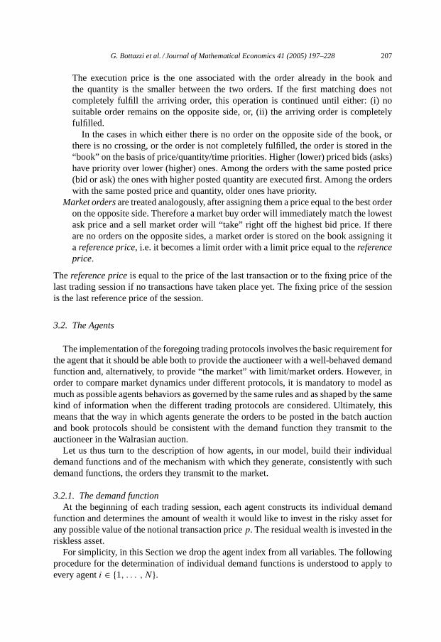
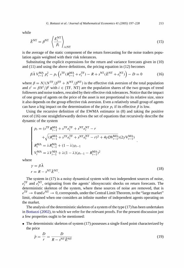
G. Bottazzi et al. / Journal of Mathematical Economics 41 (2005) 197–228 209
*p
Quantity
Price
-A
pB t - 1
t - 1
Fig. 6. An example of individual demand function forEt−1[ρt ] < R.
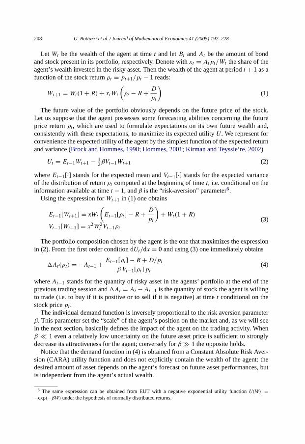
We add to (4) the restriction that agents cannot hold short positions in terms of bothassets and bonds. This means thatAt(p) must be not less then−At−1; hence if theoffered quantity of asset resulting from (4) is greater then−At−1, it is replaced by−At−1.At the same time, the demanded quantity of asset at pricep cannot be larger thenBt−1/p.The resulting demand function in general is not differentiable but does present a continuousnonincreasing behavior. Its shape depends on the sign of the differenceEt−1[ρt ] − R:illustrations are presented inFigs. 6 and 7.
3.2.2. The generation of ordersWhatever the form of the demand function, in order to trade under both batch auction
and book protocols, agents must be able to express single orders of both market and limittypes. To obtain that, we use the following procedure: when an agent is required to providean order, it picks a price at random in the neighborhood of the last asset pricept−1 and thendecides the associated quantity on the ground of its demand function. The support of thisdistribution is determined by the distance between the last price of the assetpt−1 and theagent’s individual equilibrium pricep∗, i.e. the price at which its present portfolio wouldface no rebalancingAt(p
∗) = 0. The exact procedure depends on the side of the order,i.e. whether of the buy or sell type.
For asell order, the order pricep is obtained from
log(p) = log(p∗) + ε|log(pt−1) − log(p∗)| (5)
*p
Quantity
Price
pB t-1
-At - 1
Fig. 7. An example of individual demand function forEt−1[ρt ] > R.
210 G. Bottazzi et al. / Journal of Mathematical Economics 41 (2005) 197–228
whereε is a random variable drawn from an uniform distribution on [0,1]. The associatedquantity is derived from the demand functionq = At(p). The quantity is negative asit should be for a sell order, since, according to (5),p ≥ p∗ andAt is a nonincreasingfunction ofp. If ε < η, with η ∈ [0,1] a parameter specific of the agent, the supplied orderis a market order(·,At(p)); otherwise it is a limit order(p,At(p)). The parameterηdefines the agent propensity to submit market orders: ifη = 1 all the orders are marketorders while ifη = 0 all the orders are of the limit type. Under this prescription marketorders tend to be generated with prices nearer top∗ and, consequently, they entail smallerquantities.
Analogously, for abuy orderthe price is obtained by
log(p) = log(p∗) − ε|log(pt−1) − log(p∗)| (6)
whereε has the same meaning as above. Notice that a buy order can in principle be issuedby agents owning no asset, i.e.A = 0. In this casep∗ does not exist and the following ruleis used instead
log(p) = log(pt−1) − ε|log(pt−2) − log(pt−1)| (7)
The subsequent determination of the order quantity and the decision whether to submit alimit or a market order is undertaken following the same rules as of the sell-type decision.
Notice that, according to this whole procedure, the generated limits order(p,At(p))
are points which always lay on the agents demand function. Moreover, the requirementthat agents take into consideration the last price of the asset to generate prices for theirorders is consistent with the idea of maximizing the probability of the order to befulfilled.
3.3. Agents typologies
The form of the demand function assumed in (4) is consistent with the agent budget-constraint and depends only on the parameterβ, measuring the agent risk aversion, and onthe agent’s forecasts about future asset prices, captured by the two expectationsEt−1[ρt ]andVt−1[ρt ].
In this paper we confine our attention to the case where the agents belong to two generictypes, meant to be stylized metaphors of two different trading patterns, which we calltrend followersandnoise traders. Both types believe in the existence of some underlyingstochastic process describing the dynamics of prices and form their expectations aboutthe mean and variance of future returns on the ground of their distinct “visions of theworld”.
3.3.1. Trend followersTrend followers assume that price dynamics follow a (geometric), almost stationary,
Brownian motion and that future returns can be predicted on the base of past history us-ing some consistent statistical estimator. More precisely, in their forecasting of return andvolatility, they behave as naıve econometricians, using the exponentially weighted mov-ing average (EWMA) of returnRMA
t−1 in order to obtain the forecast for the return, and the
G. Bottazzi et al. / Journal of Mathematical Economics 41 (2005) 197–228 211
exponentially weighted sample variance of past returnsVMAt−1 for the prediction of variance.
The EWMA estimatesRMAt−1 andVMA
t−1 are defined as follows:
RMAt−1 = (1 − λ)
∑∞τ=2 λ
τ−2ρt−τ
VMAt−1 = (1 − λ)
∑∞τ=2 λ
τ−2[ρt−τ − RMAt−1]2
(8)
whereλ ∈ (0,1) is a measure of the length of the memory of the agent: the smallerλ, thelower the relative weight of observations far from the past. Notice that these expressions areanalogous to the one proposed by the RiskMetricsTM group (seeLongerstaey et al., 1996),and widely applied by actual operators in their forecasting activity7. The estimates in (8)also admit a recursive form:
RMAt−1 = λRMA
t−2 + (1 − λ)ρt−2
VMAt−1 = λVMA
t−2 + λ(1 − λ)(ρt−2 − RMAt−2)
2.(9)
In order to differentiate among different trend followers, we introduce a source of idiosyn-cratic noise affecting agents’ individual forecasts. We assume that the forecasts by trendfollowers are noisy version of the EWMA estimator and set
ETFt−1[ρt ] = RMA
t−1 + εTFt
VTFt−1[ρt ] = VMA
t−1
(10)
whereεTF is an i.i.d. random variable, with zero mean, independently generated for eachagent at each time step.
3.3.2. Noise tradersNoise traders are assumed to have a pure-noise forecasting rule for future price returns
while they follow the same rule as trend followers concerning the estimation of futurevariance:
ENTt−1[h(t)] = ENT + εNT
t
VTFt−1[h(t)] = VMA
t−1
(11)
whereεNT is a random variable with the same structure ofεTF andENT is a fixed parameter,different for different agents, which describes a static idiosyncratic component of noisetraders forecast. The value ofENT is randomly and independently generated for each agentat the beginning of the simulation and kept fixed along the whole simulation history.
Notice that, within this setting, the heterogeneity inside the population of noise tradersis, in general, higher that the one among trend followers. The latter, indeed, differ onlywith respect to the idiosyncratic component in their return forecasts, while the former alsopossess different underlying (constant) estimatorsENT.
7 The RiskMetricsTMgroup actually proposes an EWMA estimator of the volatility, defined as the second momentof the returns distribution. The expression above represents its natural extension to the central moments.
212 G. Bottazzi et al. / Journal of Mathematical Economics 41 (2005) 197–228
4. A benchmark: the “large market” limit
Before comparing the different types of trading protocols it is revealing to analyze thedynamics of the market in the particular case in which prices are set via a Walrasian mecha-nism and no budget constraint on the agents positions is assumed, i.e. agents can take shortpositions in both the risky asset and the riskless bond.
In total generality, under these assumptions, it is possible to directly derive the assetpricing equation from the demand curve in (4). After some algebra, from the market clearingcondition 0= ∑
i Ai,t(p), one obtains the following quadratic equation:
p2A − p
⟨Ei,t−1[ρt ] − R
βiVi,t−1[ρt ]
⟩i
−⟨
D
βiVi,t−1[ρt ]
⟩i
= 0. (12)
whereA = ATOT/N is the average number of asset units per agent, i.e. the total amountof asset over the number of agents, and〈·〉i denotes the average of the argument on thepopulation of agents. The termA is positive and (12) has two real roots, of which only onepositive, which we take to be the pricept .Thus, the form of the utility function assumed in(2) generates demand schedules which in equilibrium yield unique and positive prices.
Incidentally, note that, in contrast withBrock and Hommes (1998), we obtain a non-linearprice equation due to the fact that we do not assume a null total supply of asset, i.e. we donot putA = 0.
If all agents expect that the price will be constant - so that they predict zero mean andzero variance for future returns - the only solution of (12) isp = D/R. This outcome can beeasily seen from (12) by taking the limitEi,t−1[ρt ] → 0 andVi,t−1[ρt ] → 0 for eachi. Thissolution corresponds to the fixed point of the dynamics of the model, and, interestingly, itdoes not depend on any behavioral parameter of the agents (in fact, it is easy to show thatit corresponds to the rational expectation equilibrium of the model).
Further properties can be uncovered by specifyingEq. (12)according to the behavioralrestrictions, deriving from traders types described inSection 3.3above.
Suppose that there areNTF trend followers andNNT noise traders operating on the market(NTF + NNT = N), characterized for simplicity by the same forecasting parameterλ. Let
βTF =(⟨
1
βi
⟩i∈TF
)−1
, βNT =(⟨
1
βi
⟩i∈NT
)−1
(13)
be the effective risk aversions of the population of trend followers and noise traders. Here〈·〉i∈TF and〈·〉i∈NT denote the average of the argument over theNTF trend followers andover theNNT noise traders, respectively. In (13) the effective risk aversion of a group ofagents is defined as the harmonic mean of the risk aversions of the agents belonging to thegroup, i.e. as the inverse of their average risk tolerance.
Next define the average idiosyncratic shocks of the two groups as the average of theforecasting shocks of the agents belonging to the groups weighted with their risk tolerances,namely
eTFt = βTF
⟨εTFi,t
βi
⟩i∈TF
, eNTt = βNT
⟨εNTi,t
βi
⟩i∈NT
(14)
G. Bottazzi et al. / Journal of Mathematical Economics 41 (2005) 197–228 213
while
ENT = βNT
⟨ENT
i
βi
⟩i∈NT
(15)
is the average of the static component of the return forecasting for the noise traders popu-lation again weighted with their risk tolerances.
Substituting the explicit expressions for the return and variance forecasts given in (10)and (11) and using the above definitions, the pricing equation in (12) becomes
βA VMAt−1 p2
t − pt
(sTF(RMA
t−1 + eTFt ) − R + sNT(ENT + eNT
t ))
− D = 0 (16)
whereβ = N/(NTF/βTF + NNT/βNT) is the effective risk aversion of the total populationandsi = βNi/βi with i ∈ {TF, NT} are the population shares of the two groups of trendfollowers and noise traders, rescaled by their effective risk tolerances. Notice that the impactof one group of agents on the price of the asset is not proportional to its relative size, sinceit also depends on the group effective risk aversion. Even a relatively small group of agentscan have a big impact on the determination of the pricept if its effectiveβ is low.
Using the recursive definition of the EWMA estimator in (8) and taking the positiveroot of (16) one straightforwardly derives the set of equations that recursively describe thedynamic of the system
pt = (sTFRMAt−1 + sTFeTF
t + sNTeNTt − r
+√(RMA
t−1 + sTFeTFt + sNTeNT
t − r)2 + 4γDVMAt−1)(2γVMA
t−1)
RMAt = λRMA
t−1 + (1 − λ)ρt−1
VMAt = λVMA
t−1 + λ(1 − λ)(ρt−1 − RMAt−1)
2
.
where
γ = βA
r = R − sNTENT.(18)
The system in (17) is a noisy dynamical system with two independent sources of noise,eTFt and eNT
t , originating from the agents’ idiosyncratic shocks on return forecasts. Thedeterministic skeleton of the system, where these sources of noise are removed, that iseTF → 0 andeNT → 0, corresponds, under the Central Limit Theorem, to the “large market”limit, obtained when one considers an infinite number of independent agents operating onthe market.
The analysis of the deterministic skeleton of a system of the type (17) has been undertakenin Bottazzi (2002), to which we refer for the relevant proofs. For the present discussion justa few properties ought to be mentioned:
• The deterministic skeleton of system (17) possesses a single fixed point characterized bythe price
p = D
r= D
R − sNTENT(19)
214 G. Bottazzi et al. / Journal of Mathematical Economics 41 (2005) 197–228
• The stability domain in the parameters’ space of this fixed point is defined by the inequality
λ + R − sNTENT
sTF > 1 (20)
• The system does, in general, possess more then one attractor, and the general (i.e. not fixedpoint) attractor of the system is a bounded set with possibly strange character, associatedwith periodic, quasi-periodic or chaotic price dynamics.
Notice that the fixed point differs from the asset fundamental valueD/R by a correctionfactor due to the aggregate impact of the noise traders’ biasesENT. If one assumes that thestatic component of the noise traders’ forecast rule is centered around zero – correspondingto a complete symmetry between overvaluation and undervaluation of future asset returns– the price at the fixed point reduces to the asset fundamental value.
From (20) it is also clear that the trend followers play a destabilizing role. When theirnumber is zero (sTF → 0) the system fixed point is always stable, provided, of course, thatthe static components of noise traders’ forecast errors is small enough to satisfyENT <
R/sNT.Finally, notice that the bounded nature of the system attracting set and the intertempo-
ral budget constraint (1) imply that, even if the total wealth of the underlying economyexponentially increases with an average rate of growth equal to the riskless returnR, theshares of wealth owned by the two populations of agents follow a cyclical behavior. In thelanguage ofDe Long et al. (1991), even if one group can possibly dominate the other, thesurvival of both groups is always guaranteed.
5. Simulation features and results
To sum up, the behavior of any generic agent in our model can be completely specifiedby just three parameters: its risk aversion,β; the time horizon over which it evaluates pastasset performances in order to build its own forecasts about price movement,λ; and itspropensity to submit market orders instead of limit orders,η (this last parameter applyingonly to markets characterized by a batch auction or book protocols).
As described above, there are two sources of heterogeneity in our model. A first one isstatic and “intrinsic” to the agents, in so far as they differ from the start in their parametersβ, λ andη. A second one is dynamic and concerns idiosyncratic shocks on the estimatesagents make. In the following analysis we shall use both forms of heterogeneity.
We consider a mixed population made ofnoise tradersandtrend followers. We set thememory parameter to the same valueλ = 0.97 for the whole population of agents. Thisvalue sets the decay characteristic time for the impact of past price dynamics on pricepresent dynamics at about 30 time steps. Thus, we expect the cyclical behavior of prices inour simulations to display a period ranging between 60 and 300 time steps, depending onthe level of noise.
The value ofβ for the different agents is randomly drawn from an uniform distributionon [106,2 × 10⁶]. This seemingly very large number is due to the fact that we normalizethe total amount of asset to 1 and the dynamic depends on the parameterγ = βA (cf. 17
G. Bottazzi et al. / Journal of Mathematical Economics 41 (2005) 197–228 215
Table 2Values of parameters used in simulation
Parameter Value
R 0.00001D 0.0002λ 0.97β U(106,2 × 10⁶)
εTF U(−0.01,0.01)εNT U(−0.05,0.05)ENT U(−0.01,0.01)Number of agents 100Transient 10,000Simulation length 5,000
and 18), i.e. the product of the population effective risk-aversion and the average numberof asset units per agent. The support of the distribution from which the values ofβ aredrawn is the same for the two groups of agents. This implies that the order of magnitudeof the aggregate demand function of the two groups is similar and the modification of theirrelative sizes does not affect the effective risk-aversion of the whole population. Moreover,the impact of the two groups on the market is simply proportional to their respective sizes.We have experimented with different support for the distribution ofβ, from β ∼ 103 to∼ 108: results happen to be robust to such variation.
The dynamic components of the agents’ heterogeneity,εTF andεNT, are randomly andindependently drawn from an uniform distribution with support [−0.01,0.01] for trend fol-lowers and [−0.05,0.05] for noise traders. The static components of noise traders forecastsENT are drawn from an uniform distribution with support [−0.01,0.01].
Finally, in order to warrant some market liquidity, we require agents to post, at the sametime, a sell and a buy order within both the batch auction and the order book protocols,following the procedure outlined inSection 3.2.2.
The values of the parameters used during the simulations are summarized inTable 2.
5.1. Market dynamics and the role of noise
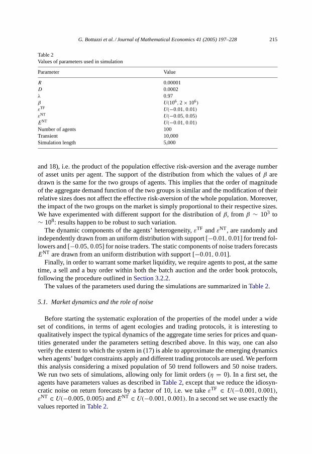
Before starting the systematic exploration of the properties of the model under a wideset of conditions, in terms of agent ecologies and trading protocols, it is interesting toqualitatively inspect the typical dynamics of the aggregate time series for prices and quan-tities generated under the parameters setting described above. In this way, one can alsoverify the extent to which the system in (17) is able to approximate the emerging dynamicswhen agents’ budget constraints apply and different trading protocols are used. We performthis analysis considering a mixed population of 50 trend followers and 50 noise traders.We run two sets of simulations, allowing only for limit orders (η = 0). In a first set, theagents have parameters values as described inTable 2, except that we reduce the idiosyn-cratic noise on return forecasts by a factor of 10, i.e. we takeεTF ∈ U(−0.001,0.001),εNT ∈ U(−0.005,0.005) andENT ∈ U(−0.001,0.001). In a second set we use exactly thevalues reported inTable 2.
216 G. Bottazzi et al. / Journal of Mathematical Economics 41 (2005) 197–228
0
0.01
0.02
0.03
0.04
0.05
0.06
0.07
0 100 200 300 400 500 600 700 800 900 1000
pric
e
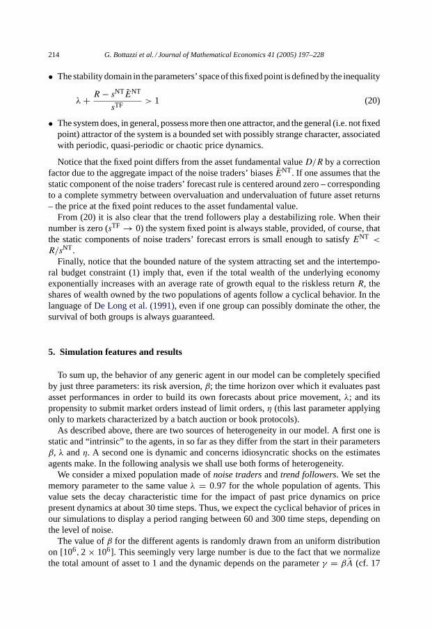
Fig. 8. Price dynamics of the deterministic skeleton of (17) withR, D andλ as inTable 2, β = 1.5 × 10⁶ andsTF = sNT = 0.5.
As shown inFig. 9, in the first set of simulations, when the idiosyncratic noise componentsare rather low, the three protocols generate a quite similar price history. InFig. 8we reportthe price time series generated directly from the deterministic version (eTF
t = eNTt = 0∀t)
of (17) withR, D andλ set according toTable 2, with sTF = sNT = 0.5 and with the riskaversion parameter taking the average value considered in simulationsβ = 1.5 × 10⁶. Asone can see, the cyclical behavior in the dynamics of (17) shown inFig. 8 still appearsin all the price series reported inFig. 9 and the average price is roughly the same for thethree protocols. The observed reduction in the support of price oscillations is due to thepresence of the noise, which tends to shorten the average lifetime of the market “bubbles”,i.e. the periods of steady upward trend, and, consequently, reduces the height of the pricepeaks. The reduction in the oscillations amplitude is more pronounced in the order-drivenprotocols, due to their intrinsic “noisy” nature. In fact, in the batch auction, a source ofrandomness is present at the level of the order generation mechanism while in the bookprotocol, a further source of noise derives from the random arrivals of agents orders.
The dynamics of traded quantities are also similar, with an increase in the volume volatilityand a decrease in the average volume levels whenever one moves from a Walrasian mecha-nism to order-driven protocols. This is easily understandable, since the Walras case allowsfor the transaction of the entire intramarginal quantity while in the other two protocols thereis a “tradable” amount of asset that remains untraded (we shall come back to this issuebelow when dealing with the allocative efficiency of different protocols).
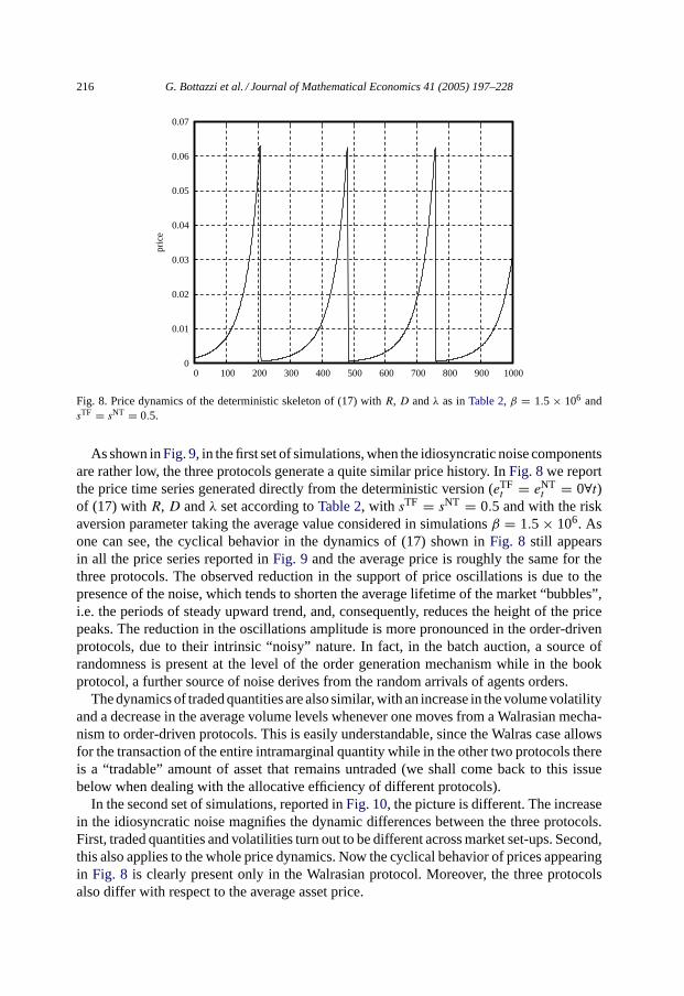
In the second set of simulations, reported inFig. 10, the picture is different. The increasein the idiosyncratic noise magnifies the dynamic differences between the three protocols.First, traded quantities and volatilities turn out to be different across market set-ups. Second,this also applies to the whole price dynamics. Now the cyclical behavior of prices appearingin Fig. 8 is clearly present only in the Walrasian protocol. Moreover, the three protocolsalso differ with respect to the average asset price.
G. Bottazzi et al. / Journal of Mathematical Economics 41 (2005) 197–228 217
Fig. 9. Price (thicker line) and quantity dynamics under the three market protocols. The simulation is performedwith 50 trend followers and 50 noise traders with parameters as reported inTable 2except for the idiosyncraticshocks, whose support is reduced to [−.001, .001] for trend followers dynamic componentεTF and the staticcomponents of noise tradersENT , and to [−0.005,0.005] for the dynamic components of noise tradersεNT.
There is an important qualitative conclusion already stemming from this ex-ercise. It is the idiosyncratic noise, capturing the fine intra-group heterogeneity ofagents, that makes the different dynamic properties of the diverse trading protocolsemerge.
Fig. 10. Price (thicker line) and quantity dynamics under the three market protocols. The simulation is performedwith 50 trend followers and 50 noise traders under the parameterization reported inTable 2.
218 G. Bottazzi et al. / Journal of Mathematical Economics 41 (2005) 197–228
With this qualitative property in mind, let us turn to a more systematic analysis of thedifferent behavioral ecologies and their interactions with the institutional frameworks.
5.2. Different trading protocols and ecologies of behaviors
We run simulations with the parameters values as reported inTable 2and, within everymarket structure, we consider the following proportions between trend followers and noisetraders: 0/100, 10/90, 20/80, 30/70, 40/60, 50/50, 60/40, 70/30, 80/20, 90/10, 100/0.
Concerning the proportion of market orders, we consider different values ofη (0, 0.1,0.2, 0.3, 0.4, 0.5), homogeneous over the population. In the course of the simulations, wediscovered that it was impossible to experiment with the full range of values (i.e.η ∈ [0,1]):for values ofη higher than 0.5 the overwhelming number of market orders generates anabnormal price volatility which eventually leads to the absence of trade for long periods oftime.
In computing the statistics which follow we use the last 5000 steps of each simulation,after discarding the first 10,000 in order to carefully avoid transient effects due to initialconditions. We have in fact checked that this transient length is large enough to let theaggregate dynamics settle around the attracting set of the underlying deterministic system(17). Moreover, the chosen simulation length allows the computation of the relevant statisticson a time scale that is one order of magnitude greater than the price cycles generated by(17) when the parameters take the values fromTable 2.
5.2.1. Comparative allocative efficiencyA crucial property of different market institutions regards their relative allocative effi-
ciency, i.e. their ability to efficiently allocate resources among traders. We begin by com-paring the revealed allocative efficiency of different trading protocols.
Were one to know the traders’ demand functions, a natural measure of allocative efficiencyunder periodic auction protocols would be the aggregate surplus of buyers and sellers (seeGode and Sunder, 1997). However, since we also want to compare continuous auctionmarket mechanisms, such a notion of aggregate surplus cannot be applied and an alternativemeasure has to be devised. To this purpose just take the outcome of a notional Walrasianauction as a benchmark and define a measure of “efficiency loss”L for agenti at timet as
Li,t = 1 − 1
1 + |Ai,t(pt) − Ai,t|pt
(21)
whereAi,t(pt) = Ai,t−1 + Ai,t(pt) is the agents’ desired quantity of asset at pricept
andAi,t is the amount of asset that the agent possesses at the end of the trading session.This measure expresses the distance of the agent’s post-trade position on the market fromthe optimal one, given its demand function and the prevailing asset price. The possiblevalues ofL range between 0 and 1. Indeed if the agent participation to the market led it to amarket position laying on its individual demand function, this would implyAi,t(pt) = Ai,t
and consequentlyLi,t = 0. Notice that this outcome is automatically guaranteed when thetrading protocol is a Walrasian auction. Conversely, if the agent, at the end of the tradingsession, finds itself far from its individual demand curve, the difference|Ai,t(pt) − Ai,t|increases and, in the absence of budget constraints, it can become infinite, so thatLi,t = 1.
G. Bottazzi et al. / Journal of Mathematical Economics 41 (2005) 197–228 219
From expression (21) we can compute the aggregate loss of efficiency as the sum of theindividual losses
Lt =N∑i=1
Li,t (22)
over theN agents. For our present purposes, this measure exhibits two advantages withrespect to the aggregate surplus used by(Gode and Sunder, 1997). First, as already men-tioned, it can be applied to any trading protocol, since it only uses the end-of-trade assetprice and end-of-trade positions of the agents. Second, it considers both intra-marginal andextra-marginal traders. This is crucial because in an order-driven protocol a trader may finditself in an extra-marginal position due to the order it originally issued, notwithstanding thefact that it would have chosen to participate at the price at which trade actually happens totake place.
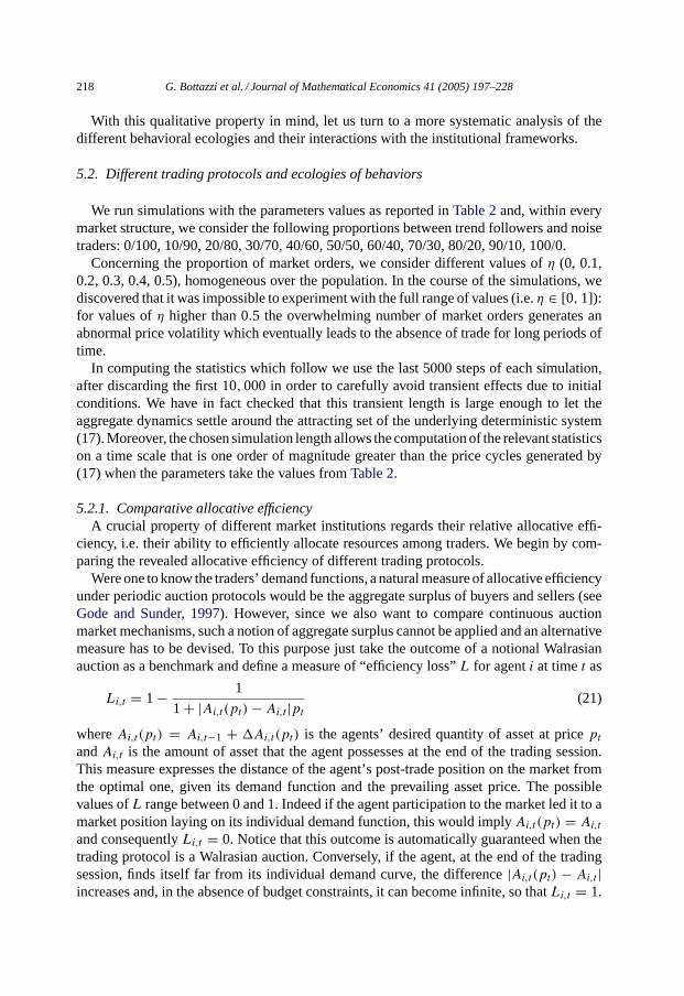
We have computed the average aggregate loss of efficiencyL in the simulation experi-ments under both batch auction and order book protocols: the results are reported inFig. 11.Notice, first, that the allocative efficiency is relatively insensitive to the particular ecologyof agents operating on the market, while it is extremely sensitive to the parameterη thatdescribes the share of market orders issued by the agents themselves. Interestingly, thecomparative efficiency of the alternative market architectures turns out to crucially dependupon this parameter.
Under both batch and order book protocols, the loss of efficiency generally increaseswith η. In fact, market orders bear two conflicting influences upon allocative efficiency.On one hand, since they do not entail any constraint on transaction prices, they may yieldpost-trade positions which are very far from the agents’ demand curves. On the other
Fig. 11. The allocative efficiency of the order book and batch auction protocols for different ecologies of agentsand different share of market orders.
220 G. Bottazzi et al. / Journal of Mathematical Economics 41 (2005) 197–228
hand, they facilitate the matching of orders and they increase market liquidity, reducing thesource of efficiency loss due to involuntary exclusion from trade. The ways the two effectscombine depend upon the specific architectures and affect in nonlinear ways the allocativeefficiency of the market. Under the order book protocol, for low levels ofη, a rise in thelatter induces no or very low efficiency loss. However, for higher proportions of marketorders, the probability for them to be traded against “abnormal” limit orders increases and,with that, also volatility and market inefficiency. Prices resulting from a match betweena market order and an “abnormal” limit order are likely to generate market positions forissuers of the market orders which are far from their demand curves. Moreover, the ensuing“abnormal” prices tend to hinder subsequent trade. Thus, for higher levels ofη, allocativeinefficiency grows faster.
Conversely, in the batch auction the foregoing trade-off between liquidity and volatilitydisappears. Abnormal limit orders are automatically prevented from trading by the auctionmechanism itself, which, at the same time “forces”, so to speak, the liquidity of the market.Thus, the overwhelming effect of market orders is to loosen the control of traders uponactual trading prices. Consequently, the allocative inefficiency steadily increases withη.
5.2.2. Comparative statistical properties of market dynamicsIn line with the empirical evidence discussed inSection 2, let us analyze the statistics
concerning skewness, kurtosis, autocorrelation of returns and volatility clustering.It is remarkable that the simulation results, notwithstanding the utter simplicity of the
model, most often display comparative properties in tune with those of actual financialmarkets, both in terms of sign and even in the (rough) orders of magnitude.
We first discuss results forη = 0 (that is, only limit orders are allowed) and, next,highlight the impact of an increasing possibility to place market orders.
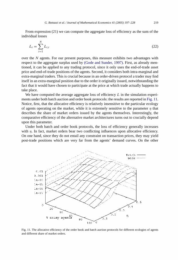
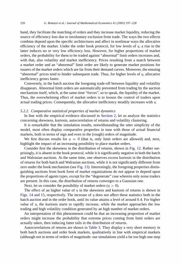
Consider first the skewness in the distribution of returns, shown inFig. 12. Rather sur-prisingly, it is absent in the book protocol, while it is significantly negative in both the batchand Walrasian auctions. At the same time, one observes excess kurtosis in the distributionof returns for both batch and Walrasian auctions, while it is not significantly different fromzero under the book mechanism (seeFig. 13). Interestingly, the foregoing properties distin-guishing auctions from book form of market organizations donot appear to depend uponthe proportions of agents types, except for the “degenerate” case wherein only noise tradersare present. In this case, the distribution of returns converges to a Gaussian one.
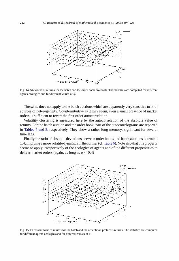
Next, let us consider the possibility of market orders (η > 0).The effect of an higher value ofη in the skewness and kurtosis of returns is shown in
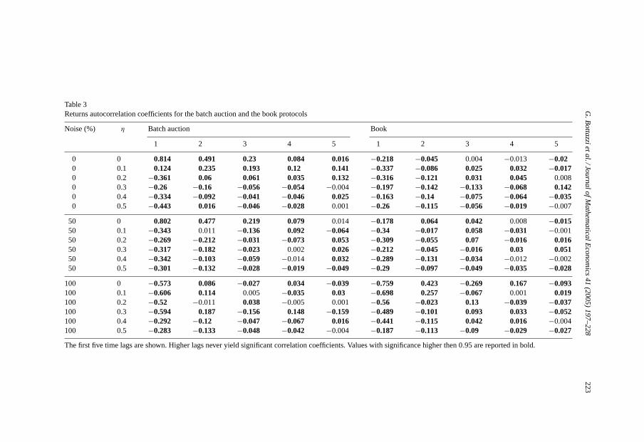
Figs. 14 and 15, respectively. The increase ofη does not affect these statistics both in thebatch auction and in the order book, until its value attains a level of around 0.4. For highervalue ofη, the kurtosis starts to rapidly increase, while the market approaches the lowtrading and high volatility condition generated by an high number of market orders.
An interpretation of this phenomenon could be that an increasing proportion of marketorders might increase the probability that extreme prices coming from limit orders areactually taken, then inducing fatter tails in the distribution of returns.
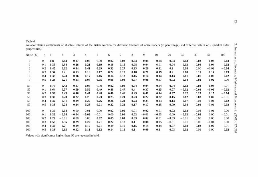
Autocorrelations of returns are shown inTable 3. They display a very short memory inboth batch auctions and order book markets, qualitatively in line with empirical markets(although not in terms of orders of magnitude: our simulations yield a far too high one-step
G. Bottazzi et al. / Journal of Mathematical Economics 41 (2005) 197–228 221
Fig. 12. Skewness of returns for the Walrasian auction, the batch auction and the order book for different proportionsof agents types.
autocorrelation). Moreover it is rather striking that the one lag negative autocorrelation forthe order book seems independent from both the ecology of agents and the types of orderposted and is reminiscent of the negative autocorrelation in high frequency financial marketsdue to price bounces featured by continuous auctions (seeGoodhart and Figliuoli, 1991).
Fig. 13. Excess kurtosis of returns for the Walrasian auction, the batch auction and the order book for differentproportions of agents types.
222 G. Bottazzi et al. / Journal of Mathematical Economics 41 (2005) 197–228
Fig. 14. Skewness of returns for the batch and the order book protocols. The statistics are computed for differentagents ecologies and for different values ofη.
The same does not apply to the batch auctions which are apparently very sensitive to bothsources of heterogeneity. Counterintuitive as it may seem, even a small presence of marketorders is sufficient to revert the first order autocorrelation.
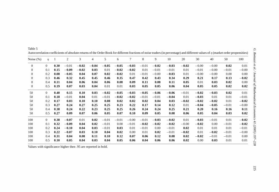
Volatility clustering is measured here by the autocorrelation of the absolute value ofreturns. For the batch auction and the order book, part of the autocorrelograms are reportedin Tables 4 and 5, respectively. They show a rather long memory, significant for severaltime lags.
Finally the ratio of absolute deviations between order books and batch auctions is around1.4, implying a more volatile dynamics in the former (cf.Table 6). Note also that this propertyseems to apply irrespectively of the ecologies of agents and of the different propensities todeliver market orders (again, as long asη ≤ 0.4)
Fig. 15. Excess kurtosis of returns for the batch and the order book protocols returns. The statistics are computedfor different agents ecologies and for different values ofη.
G.B
otta
zzieta
l./Jou
rna
lofM
ath
em
atica
lEco
no
mics
41
(20
05
)1
97
–2
28
223
Table 3Returns autocorrelation coefficients for the batch auction and the book protocols
Noise (%) η Batch auction Book
1 2 3 4 5 1 2 3 4 5
0 0 0.814 0.491 0.23 0.084 0.016 −0.218 −0.045 0.004 −0.013 −0.020 0.1 0.124 0.235 0.193 0.12 0.141 −0.337 −0.086 0.025 0.032 −0.0170 0.2 −0.361 0.06 0.061 0.035 0.132 −0.316 −0.121 0.031 0.045 0.0080 0.3 −0.26 −0.16 −0.056 −0.054 −0.004 −0.197 −0.142 −0.133 −0.068 0.1420 0.4 −0.334 −0.092 −0.041 −0.046 0.025 −0.163 −0.14 −0.075 −0.064 −0.0350 0.5 −0.443 0.016 −0.046 −0.028 0.001 −0.26 −0.115 −0.056 −0.019 −0.007
50 0 0.802 0.477 0.219 0.079 0.014 −0.178 0.064 0.042 0.008 −0.01550 0.1 −0.343 0.011 −0.136 0.092 −0.064 −0.34 −0.017 0.058 −0.031 −0.00150 0.2 −0.269 −0.212 −0.031 −0.073 0.053 −0.309 −0.055 0.07 −0.016 0.01650 0.3 −0.317 −0.182 −0.023 0.002 0.026 −0.212 −0.045 −0.016 0.03 0.05150 0.4 −0.342 −0.103 −0.059 −0.014 0.032 −0.289 −0.131 −0.034 −0.012 −0.00250 0.5 −0.301 −0.132 −0.028 −0.019 −0.049 −0.29 −0.097 −0.049 −0.035 −0.028
100 0 −0.573 0.086 −0.027 0.034 −0.039 −0.759 0.423 −0.269 0.167 −0.093100 0.1 −0.606 0.114 0.005 −0.035 0.03 −0.698 0.257 −0.067 0.001 0.019100 0.2 −0.52 −0.011 0.038 −0.005 0.001 −0.56 −0.023 0.13 −0.039 −0.037100 0.3 −0.594 0.187 −0.156 0.148 −0.159 −0.489 −0.101 0.093 0.033 −0.052100 0.4 −0.292 −0.12 −0.047 −0.067 0.016 −0.441 −0.115 0.042 0.016 −0.004100 0.5 −0.283 −0.133 −0.048 −0.042 −0.004 −0.187 −0.113 −0.09 −0.029 −0.027
The first five time lags are shown. Higher lags never yield significant correlation coefficients. Values with significance higher then 0.95 are reported in bold.
224G
.Bo
ttazzie
tal./Jo
urn
alo
fMa
the
ma
ticalE
con
om
ics4
1(2
00
5)
19
7–
22
8
Table 4Autocorrelation coefficients of absolute returns of the Batch Auction for different fractions of noise traders (in percentage) and different valuesof η (market orderpropensities)
Noise (%) η 1 2 3 4 5 6 7 8 9 10 20 30 40 50 100
0 0 0.8 0.44 0.17 0.05 0.00 −0.02 −0.03 −0.04 −0.04 −0.04 −0.04 −0.03 −0.03 −0.03 −0.030 0.1 0.35 0.34 0.26 0.21 0.19 0.18 0.15 0.08 0.04 0.01 −0.04 −0.03 −0.04 −0.04 −0.020 0.2 0.45 0.22 0.34 0.41 0.39 0.33 0.27 0.23 0.26 0.31 0.2 0.08 0.00 −0.01 −0.040 0.3 0.34 0.2 0.13 0.16 0.17 0.22 0.19 0.18 0.21 0.19 0.2 0.18 0.17 0.14 0.130 0.4 0.33 0.23 0.16 0.17 0.16 0.14 0.13 0.15 0.14 0.14 0.13 0.11 0.07 0.09 0.020 0.5 0.28 0.21 0.13 0.08 0.05 0.06 0.03 0.07 0.08 0.07 0.02 0.04 0.02 0.02 0.00
50 0 0.79 0.43 0.17 0.05 0.00 −0.02 −0.03 −0.04 −0.04 −0.04 −0.04 −0.03 −0.03 −0.03 −0.0150 0.1 0.64 0.57 0.59 0.59 0.49 0.48 0.47 0.4 0.37 0.35 0.07 −0.02 −0.03 −0.03 −0.0250 0.2 0.53 0.43 0.46 0.47 0.48 0.48 0.46 0.45 0.41 0.44 0.37 0.32 0.25 0.15 −0.0450 0.3 0.39 0.23 0.22 0.2 0.23 0.23 0.24 0.23 0.22 0.22 0.15 0.12 0.03 0.02 −0.0150 0.4 0.42 0.31 0.29 0.27 0.26 0.26 0.24 0.24 0.25 0.23 0.14 0.07 0.01 −0.01 0.0250 0.5 0.38 0.24 0.24 0.23 0.21 0.22 0.21 0.17 0.17 0.15 0.09 0.04 0.04 −0.01 −0.02
100 0 0.35 0.04 0.00 0.01 0.00 −0.02 −0.02 0.01 0.02 −0.01 0.02 0.02 −0.01 −0.01 0.00100 0.1 0.32 −0.04 −0.04 −0.02 −0.01 0.00 0.04 0.03 −0.01 −0.03 0.00 −0.03 −0.02 0.00 −0.01100 0.2 0.29 −0.01 0.00 0.00 0.02 0.05 0.04 0.03 0.02 0.01 −0.03 −0.01 0.00 0.00 0.00100 0.3 0.59 0.35 0.29 0.22 0.21 0.22 0.18 0.1 0.08 0.05 −0.01 0.01 0.00 −0.01 0.00100 0.4 0.36 0.2 0.19 0.17 0.21 0.19 0.16 0.15 0.14 0.14 0.07 0.08 0.03 0.02 −0.01100 0.5 0.33 0.15 0.12 0.11 0.12 0.14 0.15 0.1 0.09 0.1 0.03 0.02 0.01 0.00 0.02
Values with significance higher then.95 are reported in bold.
G.B
otta
zzieta
l./Jou
rna
lofM
ath
em
atica
lEco
no
mics
41
(20
05
)1
97
–2
28
225
Table 5Autocorrelation coefficients of absolute returns of the Order Book for different fractions of noise traders (in percentage) and different values ofη (market order propensities)
Noise (%) η 1 2 3 4 5 6 7 8 9 10 20 30 40 50 100
0 0 0.30 −0.01 −0.02 −0.04 −0.05 −0.05 −0.03 −0.01 −0.02 −0.03 −0.02 −0.00 −0.00 0.02 0.010 0.1 0.15 −0.09 −0.02 0.03 0.01 −0.02 −0.02 0.01 −0.01 −0.01 0.01 −0.01 −0.00 −0.01 −0.000 0.2 0.08 −0.05 0.04 0.07 0.02 −0.02 0.01 −0.01 −0.00 −0.03 0.01 −0.00 −0.00 0.00 0.000 0.3 0.46 0.32 0.45 0.45 0.46 0.35 0.47 0.42 0.43 0.34 0.29 0.21 0.17 0.13 −0.020 0.4 0.11 0.04 0.06 0.04 0.06 0.08 0.09 0.11 0.08 0.11 0.05 0.01 0.03 0.02 0.000 0.5 0.19 0.07 0.03 0.04 0.01 0.01 0.03 0.05 0.05 0.06 0.04 0.05 0.05 0.02 0.02
50 0 0.40 0.15 0.10 0.03 −0.02 −0.05 −0.03 −0.05 −0.06 −0.06 −0.01 −0.02 −0.03 0.02 0.0150 0.1 0.18 −0.01 0.04 0.01 −0.01 −0.02 −0.02 −0.01 −0.01 −0.04 0.01 −0.03 0.01 0.01 −0.0150 0.2 0.17 0.03 0.10 0.10 0.08 0.02 0.02 0.02 0.04 0.03 −0.02 −0.02 −0.02 0.01 −0.0250 0.3 0.27 0.24 0.27 0.25 0.25 0.23 0.22 0.17 0.14 0.12 0.01 −0.04 −0.05 −0.01 −0.0050 0.4 0.38 0.24 0.22 0.23 0.25 0.25 0.26 0.24 0.24 0.25 0.21 0.20 0.16 0.16 0.1150 0.5 0.27 0.09 0.07 0.06 0.05 0.07 0.10 0.09 0.05 0.08 0.06 0.05 0.04 0.03 0.02
100 0 0.38 −0.07 0.01 0.02 −0.01 −0.01 −0.00 −0.01 −0.03 −0.02 0.01 −0.03 −0.01 0.01 −0.02100 0.1 0.32 −0.09 0.04 0.02 −0.01 0.00 −0.01 −0.02 −0.02 −0.02 −0.00 −0.02 0.00 −0.01 −0.02100 0.2 0.24 −0.10 0.04 0.03 −0.01 0.03 0.01 −0.01 0.00 −0.01 0.02 0.01 0.01 0.01 −0.01100 0.3 0.22 −0.07 0.03 0.10 0.04 0.02 0.00 0.01 0.02 −0.01 −0.02 0.01 −0.02 −0.01 −0.00100 0.4 0.31 0.04 0.08 0.11 0.10 0.12 0.07 0.06 0.12 0.08 0.02 −0.02 −0.01 −0.01 0.00100 0.5 0.10 0.05 0.04 0.03 0.04 0.05 0.06 0.04 0.06 0.06 0.02 0.00 0.03 0.01 0.01
Values with significance higher then.95 are reported in bold.
226 G. Bottazzi et al. / Journal of Mathematical Economics 41 (2005) 197–228
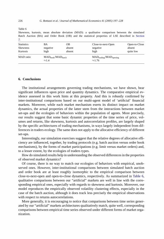
Table 6Skewness, kurtosis, mean absolute deviation (MAD): a qualitative comparison between the simulatedBatch Auction (BA) and Order Book (OB) and the statistical properties of LSE described inSection2.
Statistics BA OB Close-to-next-Open Open-to-CloseSkewness negative absent negative absentKurtosis high absent high quite low
MAD ratio MADbook/MADbatch MADtrading/MADopening
≈1.4 ≈1.76
6. Conclusions
The institutional arrangements governing trading mechanisms, we have shown, bearsignificant influences upon price and quantity dynamics. The comparative empirical ev-idence assessed in this work hints at this property. And this is robustly confirmed byinter-institutional comparisons based on our multi-agent model of ‘artificial’ financialmarkets. Moreover, while each market mechanism exerts its distinct impact on marketdynamics, the actual properties of the latter stem from the interactions between marketset-ups and the ecologies of behaviors within the population of agents. More precisely,our results suggest that some basic dynamic properties of the time series of price, vol-umes and returns, like skewness, kurtosis and autocorrelation profiles, are largely shapedby the specific architectures of trading mechanisms, in ways largely independent from dif-ferences in traders ecology. The same does not apply to the allocative efficiency of differentset-ups.
Interestingly, our simulation exercises suggest that the relative degrees of allocative effi-ciency are influenced, together, by trading protocols (e.g. batch auction versus order bookmechanisms), by the forms of market participations (e.g. limit versus market orders) and,to a lesser extent, by the ecologies of traders types.
How do simulated results help in understanding the observed differences in the propertiesof observed market dynamics?
Of course, there is no way to match our ecologies of behaviors with empirical, unob-served ones. However, inter-institutional comparisons between simulated batch auctionand order book are at least roughly isomorphic to the empirical comparison betweenclose-to-next-open and open-to-close dynamics, respectively. As summarized inTable 6,qualitative comparisons between our “artificial” markets are well in line with the corre-sponding empirical ones, especially with regards to skewness and kurtosis. Moreover, ourmodel reproduces the empirically observed volatility clustering effects, especially in thecase of the batch auction, although it does track less precisely the empirical observationswith respect to returns autocorrelations.
More generally, it is encouraging to notice that comparisons between time series gener-ated by our “artificial” markets architectures qualitatively match, quite well, correspondingcomparisons between empirical time series observed under different forms of market orga-nization.
G. Bottazzi et al. / Journal of Mathematical Economics 41 (2005) 197–228 227
Acknowledgements
We gratefully acknowledge the support of the Italian Ministry of University and Re-search (project A.AMCE.E4002GD) and S. Anna School of Advanced Studies (projectERIS02BG). Among the many insightful comments which helped in shaping the presentwork, we would like to mention in particular those by Doyne Farmer, Thorsten Hens, BlakeLeBaron, Yi-Cheng Zhang and two anonymous referees. The usual disclaimers apply.
References
Amihud, Y., Mendelson, H., 1987. Trading mechanisms and stock returns: An empirical investigation. Journal ofFinance 42, 533–553.
Arthur, W.B., Holland, J.H., LeBaron, B., Palmer, R., Tayler, P., 1997. Asset pricing under endogenous expectationsin an artificial stock market. In: Arthur, W.B., Durlauf, S.N., Lane, D.A. (Eds.), The Economy as an EvolvingComplex System II. Addison-Wesley, Boston.
Beltratti, A., Margarita, S., 1992. Simulating an Artificial Adaptive Stock Market. Mimeo, Turin University.Biais, B., Hillion, P., Spatt, C., 1999. Price discovery and learning during pre-opening period in the Paris Bourse.
Journal of Political Economy 107, 1218–1248.Bottazzi, G., 2002. A Simple Micro-Model of Market Dynamics, LEM Working Paper, Sant’Anna School of
Advanced Studies, Pisa, forthcoming in Proceedings of the Conference WEHIA 2002. Springer-Verlag, Berlin.Brock, W.A., 1997. Asset price behavior in complex environment. In: Arthur, W.B., Durlauf, S.N., Lane, D.A.
(Eds.), The Economy as an Evolving Complex System II. Addison-Wesley, Boston.Brock, W.A., de Lima, P., 1995. Nonlinear time series, complexity theory and finance. In: Maddala, G.S., Rao,
H., Vinod, H. (Eds.), Handbook of Statistics 12: Finance. North Holland, Amsterdam.Brock, W.A., Hommes, C.H., 1998. Heterogeneous beliefs and routes to chaos in a single asset pricing model.
Journal of Economic Dynamics and Control 22, 1235–1274.Calamia, A., 1999. Market Microstructure: Theory and Empirics, LEM Working Paper. Sant’Anna School of
Advanced Studies, Pisa.Campbell, J.Y., Lo, A.W., MacKinley, A.C., 1997. The Econometrics of Financial Markets. Princeton University
Press, Princeton.Chiaromonte, F., Dosi, G., 1998. Modeling a Decentralized Asset Market: An Introduction to Financial Toy-Room,
Interim Report #98015. IIASA, Laxemburg, Austria.Chiaromonte, F., Dosi, G., Jonard, N., 1998. A Speculative Centralized Asset Market with Adaptive Heterogenous
Agents, LEM Working Paper. Sant’Anna School of Advanced Studies, Pisa.Cliff, D., Bruten, J., 1997. Zero is not enough: On the Lower Limit of Agent Intelligence for Continuous Double
Auction Markets. Hewlett-Packard Laboratories, Bristol.Dacorogna, M.M., Gençay, R., Müller, U., Olsen, R.B., Pictet, O.P., 2001. An Introduction to High-Frequency
Finance. Academic Press, New York.De Long, J.B., Shleifer, A., Summers, L., Waldmann, R., 1991. The survival of noise traders in financial markets.
Journal of Business 64, 1–20.Farmer, J.D., 2002. Market force, ecology and evolution. Industrial and Corporate Change 11, 895–953.Fisher, L., 1966. Some new stock-market indexes. Journal of Business 39, 191–225.Gode, D.K., Sunder, S., 1993. Allocative efficiency of markets with zero-intelligence traders: market as a partial
substitute for individual rationality. The Journal of Political Economy 101, 119–137.Gode, D.K., Sunder, S., 1997. What makes markets allocationally efficient. Quarterly Journal of Economics 112,
603–630.Goodhart, C., Figliuoli, L., 1991. Every minute count in financial markets. Journal of International Money and
Finance 10, 23–52.Goodhart, C., Ito, T., Payne, R., 1996. One day in June 1993: a study of the workings of Reuters D2000-2 electronic
foreign exchange trading system. In: Frankel, J., Galli, G., Giovannini, A. (Eds.), The Microstructure of ForeignExchange Markets. University of Chicago Press, Chicago.
228 G. Bottazzi et al. / Journal of Mathematical Economics 41 (2005) 197–228
Guillaume, D.M., Dacorogna, M.M., Daveè, R.R., Miller, U.A., Olsen, R.B., Pictet, O.V., 1997. From the Bird’sEye to the Microscope: A Survey of New Stylized Facts of the Intra-Daily Foreign Exchange Markets. Financeand Stochastics 1, 95–129.
Hens, T., Schenk-Hoppé, K.R., Stalder, M., 2002. An application of evolutionary finance to firms listed in theSwiss market index. Swiss Journal of Economics and Statistics 138, 465–488.
Hommes, C.H., 2001. Financial markets as nonlinear adaptive evolutionary systems. Quantitative Finance 1, (1)149–167
Kirman A., Vignes, A., 1991. Price dispersion. Theoretical considerations and empirical evidence from theMarseille fish market. In: Arrow, K.J. (Eds.), Issues in Contemporary Economics. Macmillen, London.
Kirman, A., Teyssie‘re, G., 2002. Bubbles and Long Range Dependence in Asset Prices Volatilities. In: Hommes,C., Ramer, R., Withagen, C. (Eds.) Equilibrium, Markets and Dynamics, Essays in Honour of Claus Weddepohl.Springer-Verlag, Berlin.
LeBaron, B., 2000. Agent based computational finance: suggested readings and early research. Journal of EconomicDynamics and Control 24, 679–702.
Levy, H., Levy, M., Solomon, S., 2000. Microscopic Simulation of Financial Markets. Academic Press, New York.Longerstaey, J., Zangariand, A., Howard, S., 1996. RiskMetricsTM– Technical Document, 4th ed. Morgan Guaranty
Trust Company of New York, New York.Lux, T., Marchesi, M., 1999. Volatility Clustering in Financial Markets: A Micro-Simulation of Interacting Agents.
International Journal of Theoretical and Applied Finance 3, 675–702.Madhavan, A., 1992. Trading Mechanisms in Securities Markets. Journal of Finance 47, 607–642.Marengo, L., Tordjman, H., 1996. Speculation, heterogeneity and learning: a simulated model of exchange rate
dynamics. Kyklos 49, 407–437.Plott, C.R., Sunder, S., 1988. Rational expectations and the aggregation of diverse information in laboratory
securities markets. Econometrica 56, 1085–1118.Smith, V.L., Suchanek, G.L., Williams, A.W., 1988. Bubbles, crashes and endogenous expectations in experimental
spot asset markets. Econometrica 56, 1119–1151.Stoll, H., Whaley, R., 1990. Stock market structure and volatility. Review of Financial Studies 3, 37–71.Yang, J., 2001. Price-efficiency and risk sharing in two inter-dealer markets: An agent-based approach. In:
Proceedings of the Workshop on Simulations of Social Agents: Architectures and Institutions. Argonne NationalLaboratory, Argonne (Il), pp., 52–61.