input shaping for vibration-free positioning of flexible ... · 467...

467

Input shaping for vibration-free positioning of exiblesystems

M N SahinkayaDepartment of Mechanical Engineering Faculty of Engineering and Design University of Bath Claverton DownBath BA2 7AY UK

Abstract Input shaping is a simple and eVective method for reducing the residual vibration whenpositioning lightly damped systems and it remains an active research area In this paper a continuousand diVerentiable function is introduced to de ne the desired motion and then the input is shapedby inverse dynamic analysis In the proposed method the only parameter that needs to be de ned isthe output speed which is limited only by the physical constraints of the drive system The calculationof an optimum speed is demonstrated by simulation examples It is also shown that under certaincircumstances the process can be further simpli ed and the need for inverse dynamics is eliminated

Keywords input shaping open-loop control vibration control trajectory inverse dynamics

NOTATION ( )min ( )max minimum and maximum values( ) indicates unknown true values

c damping coeYcientf (t ) input force

1 INTRODUCTIONF(u) normalized input forceJ(acirc) function to be limited

In many machines load positioning is achieved byJL limiting valuesimple open-loop control In the case where structuralk stiVness coeYcient exibility is signi cant and the load is lightly dampedm massthe vibration may be unacceptable and a number oft timepapers have reported various approaches to use inputT

Ssettling time

shaping to control the vibrationu normalized timeOne approach is to divide a step input demand intox(t) xAacute (t) x(t) output displacement velocity and

smaller steps delayed in time [1 ] termed lsquoposicastrsquo con-accelerationtrol and this has been applied to exible systems [2 ]X(u) XAacute (u) X(u) normalized output displacementThe use of bang-bang control for time-optimal responsevelocity and accelerationis well established [3 ] The most popular technique fory(t) yAacute (t) y(t) input displacement velocity andinput shaping is to convolve a sequence of impulses andaccelerationvarious methods for shaping impulse sequences andY(t) YAacute (u) Y(u) normalized input displacementexamining their robustness have been reported (eg ref-velocity and accelerationerences [4 ] to [7 ] ) and applied to exible spacecraft

aacute motion speed parameter [8ndash10 ] robots [11 ] and to the control of swing of sus-acirc relative motion speed parameter pended objects transported by cranes [7 ] In order toaring( ) error function increase the rise time when using impulse shaping theuacute damping ratio impulses are allowed to take negative values [12 ] andr percentage band used in the multihump shaping of the impulses can be used to

de nition of settling time increase the system robustness [13 ] The use of a rampedoumln natural frequency sinusoid as a forcing input has also been considered

[14 15 ] The design of impulse sequences as input func-tions has been extended to multimode systems [16 17 ]The MS was received on 11 September 2000 and was accepted after

revision for publication on 19 March 2001 and to multi-input systems [18 19 ] and adaptive

I06400 copy IMechE 2001 Proc Instn Mech Engrs Vol 215 Part I

468 M N SAHINKAYA

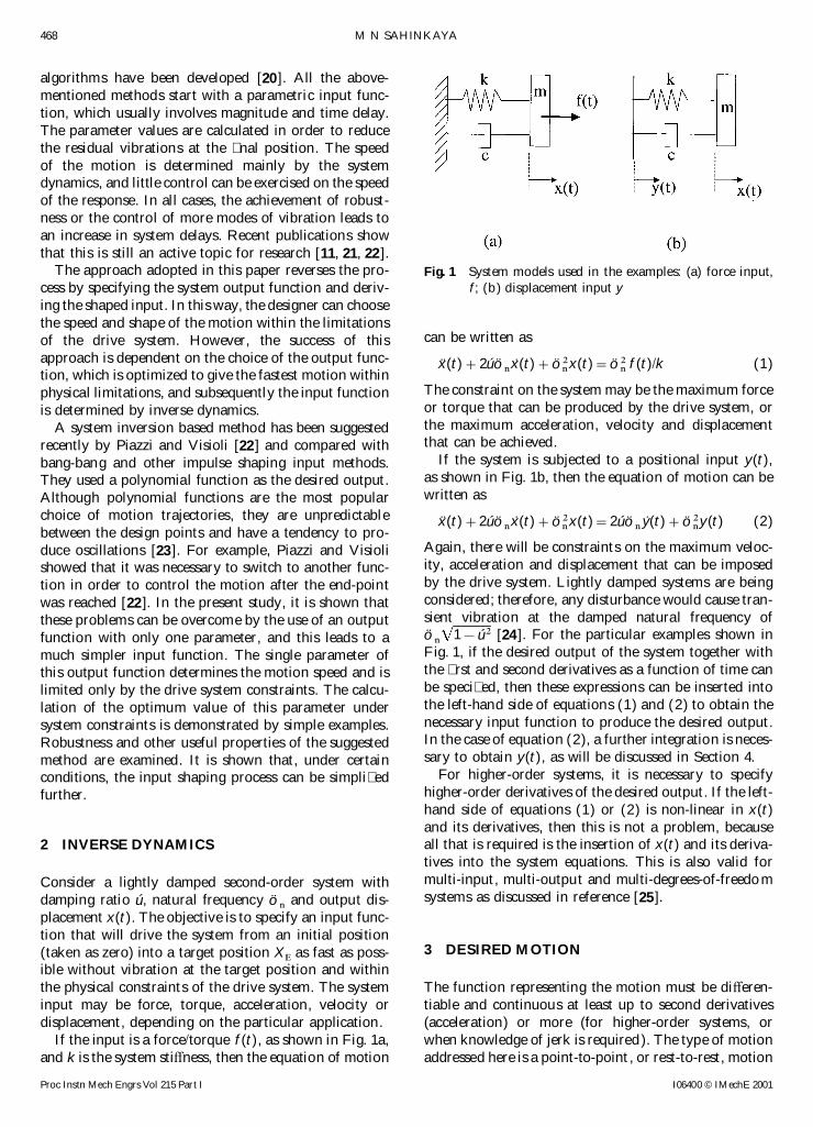
algorithms have been developed [20 ] All the above-mentioned methods start with a parametric input func-tion which usually involves magnitude and time delayThe parameter values are calculated in order to reducethe residual vibrations at the nal position The speedof the motion is determined mainly by the systemdynamics and little control can be exercised on the speedof the response In all cases the achievement of robust-ness or the control of more modes of vibration leads toan increase in system delays Recent publications showthat this is still an active topic for research [11 21 22 ]

The approach adopted in this paper reverses the pro- Fig 1 System models used in the examples (a) force inputf (b) displacement input ycess by specifying the system output function and deriv-

ing the shaped input In this way the designer can choosethe speed and shape of the motion within the limitations

can be written asof the drive system However the success of thisapproach is dependent on the choice of the output func- x(t)+2uacuteoumlnxAacute (t)+ouml2nx(t)=ouml2n f (t)k (1)tion which is optimized to give the fastest motion within

The constraint on the system may be the maximum forcephysical limitations and subsequently the input functionor torque that can be produced by the drive system oris determined by inverse dynamicsthe maximum acceleration velocity and displacementA system inversion based method has been suggestedthat can be achievedrecently by Piazzi and Visioli [22 ] and compared with

If the system is subjected to a positional input y(t)bang-bang and other impulse shaping input methodsas shown in Fig 1b then the equation of motion can beThey used a polynomial function as the desired outputwritten asAlthough polynomial functions are the most popular

choice of motion trajectories they are unpredictable x(t)+2uacuteoumlnxAacute (t)+ouml2nx(t)=2uacuteoumlnyAacute (t)+ouml2ny(t) (2)between the design points and have a tendency to pro-

Again there will be constraints on the maximum veloc-duce oscillations [23 ] For example Piazzi and Visioliity acceleration and displacement that can be imposedshowed that it was necessary to switch to another func-by the drive system Lightly damped systems are beingtion in order to control the motion after the end-pointconsidered therefore any disturbance would cause tran-was reached [22 ] In the present study it is shown thatsient vibration at the damped natural frequency ofthese problems can be overcome by the use of an outputoumln

1 shy uacute2 [24 ] For the particular examples shown infunction with only one parameter and this leads to aFig 1 if the desired output of the system together withmuch simpler input function The single parameter ofthe rst and second derivatives as a function of time canthis output function determines the motion speed and isbe speci ed then these expressions can be inserted intolimited only by the drive system constraints The calcu-the left-hand side of equations (1) and (2) to obtain thelation of the optimum value of this parameter undernecessary input function to produce the desired outputsystem constraints is demonstrated by simple examplesIn the case of equation (2) a further integration is neces-Robustness and other useful properties of the suggestedsary to obtain y(t) as will be discussed in Section 4method are examined It is shown that under certain

For higher-order systems it is necessary to specifyconditions the input shaping process can be simpli edhigher-order derivatives of the desired output If the left-furtherhand side of equations (1) or (2) is non-linear in x(t)and its derivatives then this is not a problem becauseall that is required is the insertion of x(t) and its deriva-2 INVERSE DYNAMICStives into the system equations This is also valid formulti-input multi-output and multi-degrees-of-freedomConsider a lightly damped second-order system withsystems as discussed in reference [25 ]damping ratio uacute natural frequency oumln and output dis-

placement x(t) The objective is to specify an input func-tion that will drive the system from an initial position

3 DESIRED MOTION(taken as zero) into a target position XE as fast as poss-ible without vibration at the target position and withinthe physical constraints of the drive system The system The function representing the motion must be diVeren-

tiable and continuous at least up to second derivativesinput may be force torque acceleration velocity ordisplacement depending on the particular application (acceleration) or more (for higher-order systems or

when knowledge of jerk is required) The type of motionIf the input is a forcetorque f (t) as shown in Fig 1aand k is the system stiVness then the equation of motion addressed here is a point-to-point or rest-to-rest motion

I06400 copy IMechE 2001Proc Instn Mech Engrs Vol 215 Part I

469INPUT SHAPING FOR VIBRATION-FREE POSITIONING OF FLEXIBLE SYSTEMS

where the velocity and acceleration at the start and at t=TS

the arrival of the destination are zero and remain zeroie x(t)=XE C6 A t

TSB5shy 15 A t

TSB4

+10 A t

TSB3D

0 aring t aring TS

(4)

For t=0

x(0)=0 xAacute (0)= x(0)=0

For t TS

x(TS)=XE xAacute (TS)= x(TS)=0

However this function does not satisfy the conditionsfor tgtTS and shoots oV to in nity The inverse dynamicanalysis cannot be stopped at t=TS as the settling of

(3)the system input may take longer than TS in order toreduce the vibration at the end-position Therefore thewhere TS is the settling time which should be minimized

subject to system constraints The function should be corresponding input function has to be switched toanother function such as an exponential function atsmooth and in order to achieve a fast response the

velocity should not change sign during the motion t=TS as suggested in reference [22 ] in order to obtaina smooth convergence to the end-position HoweverThe most popular function for trajectory selection is

a polynomial function of time [22 23 ] The order and the switching is done at t=TS where no errors can betolerated as the whole purpose of the exercise is to reachcoeYcients of the polynomial function can be calculated

in order to satisfy the design points de ned in terms of the end-position at TS

seconds and stay there withoutany vibration This point will be discussed further indisplacement velocity or acceleration at particular time

values However no control can be exercised between Section 53It is clear that an asymptotic behaviour is desired whenand outside the design points and oscillations or asymp-

totic behaviours may occur thereby restricting the use approaching the nal position in order to stay thereand exponential functions may be a natural choiceof the function to certain time intervals For example

use of the polynomial in equation (4) as an output func- Therefore an examination will be made of the third-order exponential function for the output motion to taketion satis es the conditions in equation (3) for t=0 and

Fig 2 Characteristics of the proposed output function


470 M N SAHINKAYA

the system from zero to XE

as follows Figure 2 shows the graph of these functions against thenormalized time u Paramater aacute is the time-scaling par-

x(t)=XE(1 shy e Otilde (aacutet)3) (5)ameter and determines the speed of motion in real timeIt is the only parameter of the proposed equation ofIn order to generalize the analysis normalized (non-

dimensional ) time u is de ned as motion to be selected and this has to be limited by thesystem physical constraints

u=aacutet (6)If the settling time T

S(r) is de ned as the time required

for the system output to arrive within a certain percent-This gives the following normalized equations of thedesired motion age r of the nal value then the corresponding value

of normalized time u can be calculated from equa-tion (7) as u=144 for r=005 (5 per cent band) andX(u)=

x(t)

XE=1 shy e Otilde u3 (7)

u=166 for r=001 (1 per cent band) Then therelationship between aacute and the settling time T

SisThe derivatives are

TS(001)=166aacute and TS(005)=144aacute (9)

Larger values of aacute produce faster motion The choice ofXAacute (u)=

1

aacuteXExAacute (t )=3u2e Otilde u3

X(u)=1

aacute2XEx(t)=(6u shy 9u4)e Otilde u3

the percentage band r for the de nition of settling timewill depend on the application

The maximum value of normalized output velocity(8)

is 118 at u=088 and the maximum value of thenormalized output acceleration is 215 at u=049Expressions for higher derivatives can easily be gener-

ated the function shape is smooth and deterministic Therefore if there are restrictions on the output velocityor acceleration then from equation (8) the maximumand satis es all of the required conditions for 0 aring tlt

Fig 3 Required (shaped) input for various acirc values (uacute=01) ndash ndash ndash contribution of the second term inequation (11)



Fig 4 System response to simpli ed input frequencies for various acirc values (uacute=01)

value of aacute can be obtained as follows ship between the system speed (characterized by oumln) and

the speed of motion (characterized by aacute) In physicalterms large values of acirc de ne a motion that is slowaacutemax=

max |xAacute |118XE

or aacutemax=Smax | x |215XE

(10)relative to the system natural frequency Obviously acirccannot take zero or negative valueswhich give the minimum settling time achievable in terms

By inserting equations (7) and (8) into equation (11)of the limits of the physical values of velocity or acceler-the following expression can be obtained for the

ation Obviously if both velocity and accelerationnormalized input to produce the desired motion

are limited then the smaller of the two aacutemax valuescalculated in equation (10) should be used

F(u)=1+ A6u shy 9u4acirc2

+6uacuteu2

acircshy 1B e Otilde u3

or

F(u)=X(u)+A6u shy 9u4acirc2

+6uacuteu2

acirc B e Otilde u3

4 REQUIRED (SHAPED) INPUT

In order to obtain the required input to achieve thedesired motion the expressions for the output displace-

(13)ment velocity and acceleration in equations (7) and (8)are substituted into the normalized form of system The required input force expression consists of two termsequation (1) given by the rst term is simply the required output and the second

approaches zero in the steady state but it compensatesX(u)+2uacuteacircXAacute (u)+acirc2X(u)=acirc2F (u) (11)some of the system dynamics in order to achieve the

where acirc and normalized force F (u) are de ned as required motion The second term in equation (13) shouldbe examined more closely It is dependent on the relative

acirc=oumlnaacute

and F (u)=1

kXEf (t) (12) speed of motion acirc and the damping ratio uacute The input

function F(u) in equation (13) is plotted for diVerentvalues of acirc for uacute=01 in Fig 3 The second term inThe newly de ned parameter acirc determines the relation-


472 M N SAHINKAYA

Fig 5 Flow chart of the input shaping process

equation (13) is also plotted (dotted lines) to illustrate the The results are shown in Fig 4 for diVerent values of acircand for uacute=01 The omission of the second term did notcontribution of this term As expected for low values of

acirc (relatively fast motion) the second term dominates the cause any problem for acirc values of 8 or greater Thesimulations for other values of uacute produced similarinput and the system requires high input values (force or

torque) in order to achieve the desired motion However characteristicsHowever use of the simpli ed input also results in theat a larger value of acirc (slower motion) the second term of

equation (13) is not signi cant and oscillations disappear output not being exactly the same function as de nedby equations (7) and (8) and there may be slightIt is observed that by drawing Fig 3 with diVerent uacute and

acirc values (not included) this is valid for any uacute value if changes in the maximum acceleration and velocity of thesystem output which have to be taken into account ifacircgt8 In applications where the system is not required to

move as fast as acirclt8 owing to limitations of the drive the speed of motion is maximized by using the con-straints on the velocity and acceleration Also the set-system the whole process is further simpli ed because the

input signal is the same as the desired output displacement tling time will be slightly aVected These eVects will bedemonstrated by the examples in the next sectionand no knowledge of the system parameter values are

used ie

F(u)=X(u)=1 shy e Otilde u3 (14) 5 OPTIMUM MOTION SPEED WITHEXAMPLESIn order to test the eVect on the system response of

ignoring the second term simulations of the normalizedsystem equations as de ned by equation (1) were carried When the normalized input function has been deter-

mined to achieve the desired motion the next step is toout with the simpli ed input function in equation (14)



Fig 6 Maximum input force as a function of acirc for various values of uacute (0 01 02 03 04)

de ne aacute (or acirc) Although the above analysis produces J(acirc) Therefore whatever the physical constraints J(acirc)is in general a well-behaved exponential functionvibration-free positioning of the system for any value of

aacute in practice there will be physical constraints that limit asymptotically going to in nity when acirc approaches zeroThis simpli es the solution of equation (15) and anythe speed If the constraints are on the peak output veloc-

ity or acceleration then equation (10) can be used to set of the simple numerical methods such as NewtonndashRaphson secant or bisection [26 ] can now be used Itthe equation value of aacute and there is no need to do any

more optimization Otherwise the following procedure is also possible to plot J(acirc) against acirc to obtain the limit-ing value of acirc The design approach is shown by a owcan be adapted

The input function in equation (13) is dependent on chart in Fig 5If the function to be limited is the maximum inputacirc for a given damping ratio of the system Therefore

even if the right-hand side of the system equation (1) is force level then J(acirc) is de ned as J(acirc)=max |F(acirc u) |The maximum value of the normalized force functionin another form the physical constraints on the system

will in general be functions of acirc The equation to be J(acirc) is plotted as a function of acirc for diVerent values ofuacute in Fig 6 A normalized force value of 1 represents thesolved to nd the optimum acirc (or minimum acirc within the

constraints) is as follows steady state force (spring force) required to keep thesystem at the nal position Even with this minimum

J(acirc) shy JL=0 (15)force level required for steady state positioning thesystem could achieve acirc values of 17 (for uacute=01) Thewhere J(acirc) is the positive function to be limited and JL

is the limit value In order to keep the system within the gure shows the optimum speed achievable for diVerentforce limit values above 1 As expected the force require-de ned constraints the acirc value chosen should be equal

to or less than the value satisfying equation (15) It is ments increase with increasing motion speed (decreasingacirc) It can also be observed from Fig 6 that the maximumimportant to note the physical signi cance of acirc which

is inversely proportional to the speed of motion motion speed for a given force limit decreases withincreasing damping ratio That is faster motion can beIncreasing system speed (ie decreasing acirc) should in

general increase the value of the function to be limited obtained with lower values of damping ratio for the


474 M N SAHINKAYA

Fig 7 Required (shaped) force input and system response with limitations on the input force magnitude(example in Section 51) mdashmdash force limited to 960 N (acirc=154 ) ndash ndash ndash force limited to 800 N (acirc=174)

same force limits For a given value of Fmax it is possible 960 N (giving a nominal maximum force value of 12)the optimum acirc value can be calculated as 1542 givingeither to obtain the optimum acirc from Fig 6 or simply

solve equation (15) a value of aacute=1834 which corresponds to a settlingtime of 0090 s (for 1 per cent band) and 0078 s (forOnce the optimum acirc value is obtained as above the

value of aacute can easily be calculated from aacute=oumln acirc which 5 per cent band) The shaped input functions can bede ned as follows from equation (13)would be enough to specify the input function in physical

units The process is demonstrated by the following threef (t)=800[1+(322t+14491t2 shy 207410t4 shy 1)examples applied to the single-degree-of-freedom system

as shown in Fig 1 with the parameters set to m=1 kg timese( Otilde 1625t)3 ]k=800 Nm and c=9 N sm giving oumln=2828 rs and

to produce outputuacute=0159 as used in reference [22 ] for ease of comparisonbetween the two approaches x(t)=1 shy e( Otilde 1625t)3 for fmax=800 N (Fmax=1)

and51 Force input with limitation on the force magnitude f (t)=800[1+(4626t+20816t2 shy 427970t4 shy 1)

For the system in Fig 1a the minimum steady state force timese( Otilde 1834t)3 ]required to keep the system in the nal position is 800 N

to produce output(corresponding to a nominal force value of 1) If this istaken as the maximum force that can be achieved then x(t)=1 shy e( Otilde 1834t)3 for fmax=960 N (Fmax=12)the optimum values of acirc can be calculated as 174 givinga value of aacute=1625 which corresponds to a settling Both results are shown in Fig 7 which clearly demon-

strates that vibration-free motion is achieved withouttime of 0102 s (for 1 per cent band) and 0089 s (for5 per cent band) If the maximum force is increased to violating the input force limitation The corresponding



Fig 8 Required (shaped) force input and system response with limitations on the acceleration (example inSection 52) mdashmdash complete force input (acirc=132) ndash ndash ndash simpli ed force input (acirc=136)

velocity and acceleration curves are also included in the be larger than 8 to meet the acceleration limitations whichallows the use of a simpli ed forcing term With the simpli-same gure ed forcing function the optimum acirc is calculated to be136 by solving equation (15) as equation (10) can nolonger be used This gives an aacute value of 208 and the52 Force input with limitation on the accelerationsimpli ed input force can now be written as

The motion in the previous example is very fast and inf (t)=800( 1 shy e( Otilde 208t)3 )practice there will probably be limitations on the maxi-

mum acceleration (or velocity) that can be achieved For The output function is no longer de ned by equationthe purpose of illustration assume that the output accel- (7) although it should be very close and the relationshiperation is limited to 10 ms2 Then the optimum value of between aacute and the settling time is now brokenacirc can be calculated either directly from equation (10) Simulations were performed with the simpli ed inputor through the solution of equation (15) as acirc=132 (or function as above and the results are shown by dashedaacute=215) corresponding to a settling time of 077 s lines in Fig 8 giving a settling time of 079 s (1 per cent(1 per cent band) and 067 s (5 per cent band) as per band) and 069 s (5 per cent band) Using the simpli edequation (9) The input and corresponding output func- input function does not produce any vibrations but leadstions can be formed from equation (13) as follows to a 2ndash3 per cent loss in speed in this example which

may be acceptable considering the simpli cationsf (t)=800[x(t)+(00738t+0332t2 shy 1089t4)obtained generating the force signal

timese( Otilde 215t)3 ]

to produce output 53 Displacement input with constraints on the inputaccelerationx(t)=1 shy e( Otilde 215t)3

The results shown in Fig 8 con rm that the design objec- The system in Fig 1b is considered here For comparisonpurposes the same conditions are used as in referencetives are achieved The optimum acirc value is calculated to


476 M N SAHINKAYA

Fig 9 Maximum input acceleration as a function of acirc for the example in Section 52

[22 ] The constraint is on the input acceleration the ed input forcing If the optimization is carried out withthe simpli ed input displacement function the optimumlimiting value being 10 ms2 The relationship between

the input force function de ned in equation (13) and the acirc value can be calculated as 131 (ie aacute=216) in orderto keep the system within the acceleration limits givinginput displacement can be written as followsthe following simpli ed input displacement function

F(u)=1

kXE

[2uacuteacircYAacute (u)+acirc2Y(u)] (16)y(t)=1 shy e Otilde (216t)3

It should be noted that the simpli cation is carried onewhere Y(u) and YAacute (u) are the normalized input displace-ment [de ned as y(t)XE ] and normalized input velocity step further from the input force expression to input

displacement thus avoiding the use of equation (16)[de ned as yAacute (t)aacuteXE] respectively u is the normalizedtime as de ned previously Equation (16) is equivalent The settling time can no longer be calculated from the

value of aacute and the simulation is performed with theto passing the calculated force input function through alow-pass lter In this example equation (16) is inte- simpli ed input expression obtaining a settling time of

0755 s (1 per cent band) and 0658 s (5 per cent band)grated to obtain the Y values This is carried out fordiVerent values of acirc and the graph of maximum input The simulation results are included in Fig 10 as dashed

lines Again use of the simpli ed input function causesacceleration versus acirc values is shown in Fig 9 For maxi-mum acceleration of 10 ms2 the optimum value of acirc a speed loss of about 2ndash3 per cent but the use of simpli-

ed input displacement oVers more bene ts than in thecan be calculated as 126 giving a value of aacute=2245which corresponds to a settling time of 074 s (1 per cent previous example because the need to convert the opti-

mized force expression (13) into input displacementband) and 064 s (5 per cent band) The results are pre-sented in Fig 10 which again con rms that the design through equation (16) is also avoided

A polynomial output function is used by Piazzi andobjectives are achieved Since the value of acirc is largerthan 8 this system also quali es for the use of a simpli- Visioli for the same example [22 ] They obtained the



Fig 10 Required (shaped) displacement input signal and system response with limitations on the inputacceleration (example in Section 53) mdashmdash complete displacement input (acirc=126) ndash ndash ndash simpli eddisplacement input ( acirc=131 )

following input displacement function with an optimum position where no vibrations are tolerated The eVect ofintroducing such a sudden step change in accelerationmotion duration of T

S=0874 s

may not be striking in this example as the motion isrelatively slow and the input displacement is very closeto its steady state value but with faster motion thiswould excite vibrations at a time when they can be least

y1(t)=shy 000136 +012124t shy 039553t2+15272t3

shy 25707t4+11765t5+000136e Otilde (8009)t

for 0 aring t aring 0874

y2(t)=1 shy 000117e Otilde (8009)(t Otilde 0874)

for tgt0874

tolerated This demonstrates the problems associatedwith the use of polynomial functions which only satisfythe conditions at the design points (ie t=0 and t=TS)with behaviour between and outside these points

(17)unpredictable

As discussed in Section 3 the polynomial function forthe desired motion can only be used for t aring T

S

Therefore the input function is switched to an6 ROBUSTNESS

exponential function matching the values at t=TS However examining the input velocity and acceleration

The eVect of errors in the natural frequency and thevalues at TS gives the followingdamping ratio on the system response will be examinedfor the examples given in Section 5 Errors will be intro-yAacute 1

(0874)=010389 yAacute 2(0874)=010400

y1(0874)=075135 y2(0874)=shy 924444 duced into oumln and uacute values in equation (1) de ned bythe following error function aring( )

This produces a large spike in acceleration the acceler-ation jumps from +01 to shy 924 ms2 taking it close to aring(oumln)=

oumln

oumlnshy 1 and aring(uacute)=

uacute

uacuteshy 1 (18)

the limiting value of 10 ms2 at the arrival of the nal


478 M N SAHINKAYA

Fig 11 Overshoot as a function of errors in oumln and uacute for the low acirc value example in Section 51 (acirc=174)

where oumln

and uacute denote the unknown actual values +02 are used in the system equation (1) to calculatethe output and the overshoot and results are plotted inwhich are estimated as 28284 rs and 0159 respectively

as used in the optimization Negative values of aring( ) corre- Fig 11 The system response is more sensitive to percent-age errors in oumln compared with uacute The results also sug-spond to overestimation of the actual parameter and

positive values to underestimation After obtaining the gest that for such low values of acirc (high relative motionspeed) the parameter estimation should be done asshaped input with the estimated values of the param-

eters system equation (1) is integrated to calculate the accurately as possible One way of reducing the errorsin the estimates is to analyse the system time response ifsystem response by using oumln

[1+aring(oumln)] and uacute [1+aring(uacute)]

This is done for diVerent values of aring( ) and the vibration vibrations occur and update the estimates accordinglyFigure 12a shows the response for aring(uacute) values of shy 02properties of the output displacement are examined to

assess the eVect of errors in parameters and +02 with no errors in oumln and Fig 12b for aring(oumln)values of shy 02 and +02 with no errors in uacute It is clearAs discussed above the value of acirc plays an important

role in the input shaping process and gives an indication from these results that the ratio and the sign of errorsin parameter estimates manifest themselves quite dis-of the motion speed with reference to the system natural

frequency The examples in Sections 51 and 52 are good tinctly in the system output when compared with thedesired response Therefore the comparison of theexamples of small and large acirc values and will be used in

the sensitivity analysis desired output and the system actual output shouldreveal the direction of corrections needed in theparameter estimates

61 Low acirc values

As an example of a low acirc value case the case examined 62 Larger acirc valuesin Section 51 with an optimum acirc value of 174 and aninput force limitation of 800 N is considered DiVerent A sensitivity analysis was performed for the example in

Section 52 the optimum acirc value was calculated as 132values of aring(oumln) and aring(uacute) within the range of shy 02 and



Fig 12 EVect of errors in oumln and uacute on the system response for the low acirc value example in Section 51(acirc=174)

A similar analysis was carried out and the eVect of par- 7 CONCLUSIONameter errors on the output overshoot is presented inFig 13 System sensitivity to errors in uacute is eVectively zero A new approach to input shaping is introduced Instead[overshoot value of about 67times10 Otilde 6 m for aring(uacute)=shy 02 of selecting a suitable form for the input function andand 47times10 Otilde 7 m for aring(uacute)=+02 for a motion of 1 m] shaping it to eliminate system vibrations a suitable formThe response is also insensitive to underestimation of for the output motion is developed and then the inputnatural frequency positive aring(oumln

) values [giving an over- is shaped to produce the desired output by inverseshoot value of 6times10 Otilde 7 m for aring(oumln)=+02] However dynamics The desired output function is based on aalthough very small higher sensitivity is observed for third-order exponential function which satis es all ofoverestimating the oumln value [overshoot of 56times10 Otilde 5 m the requirements for system positioning This method offor aring(oumln)=shy 02] Overestimating oumln means that the input shaping requires the selection of only one param-actual acirc value is smaller than that used in the optimiz- eter namely the speed Although the analysis providesation and care should be taken to avoid it Obviously vibration-free positioning of the system with any speedunderestimation of oumln

will result in slower motion than in practice the system speed is restricted by the actuatorcan be achieved constraints An optimization method is developed to

The eVect of parameter errors on the time response of obtain the maximum speed parameter in order to keepthe system is negligible and cannot be distinguished on the system within its physical constraints It is showna graphical representation when compared with the that for speeds slower than a certain value the wholedesired response Obviously similar sensitivity analysis process can be further simpli ed and even the need forwill be valid for the example in Section 53 as the acirc inverse dynamics can be eliminated

Robustness is evaluated by a sensitivity analysis onvalued used there was 126


480 M N SAHINKAYA

Fig 13 Overshoot as a function of errors in oumln and uacute for the high acirc value example in Section 52 (acirc=126)

5 Tzes A and Yurkovich S An adaptive input shaping con-the simulated examples and good tolerance towards thetrol scheme for vibration suppression in slewing exibleparameter errors is shown The advantages of the pro-structures IEEE Trans Control Syst Technol 1993posed desired motion over the polynomial choice of1(2) 114ndash121trajectories are also discussed

6 Singhose W Seering W and Singer N Residual vibrationreduction using vector diagrams to generate shaped inputsTrans ASME J Mech Des 1994 116 654ndash659

ACKNOWLEDGEMENT 7 Cho J K and Park Y S Vibration reduction in exiblesystems using a time-varying impulse sequence Robotica1995 13 305ndash313The author gratefully acknowledges the nancial sup-

8 Aspinwall D M Acceleration pro les for minimizingport of the Engineering and Physical Science Researchresidual response Trans ASME J Dynamic SystCouncil under Grant GRM97503Measmt and Control 1980 102 3ndash6

9 Tuttle T D and Seering W P Experimental veri cationof vibration reduction in exible spacecraft using inputREFERENCES shaping J Guidance Control and Dynamics 199720(4) 658ndash664

1 Smith O J M Feedback Control Systems 1958 (McGraw- 10 Singhose W Bohlke K and Seering W Fuel-eYcientHill New York) pulse command pro les for exible spacecraft J Guidance

2 Cook G Control of exible structures via posicast In Control and Dynamics 1996 19 (4) 945ndash960Proceedings of 1986 Southeast Symposium on System 11 Alici G Kapucu S and Baysec S On preshaped referenceTheory Knoxville Tennessee 1986 pp 31ndash35 inputs to reduce swing of suspended objects transported

3 Meckl P and Seering W Active damping in a three-axis with robot manipulators Mechatronics 2000 10 609ndash626robotic manipulator Trans ASME J Vibr Acoust 12 Singhose W E Seering W P and Singer N C Time-Stress and Reliability in Des 1985 107 38ndash46 optimal negative input shapes Trans ASME J Dynamic

4 Singer N C and Seering W P Preshaping command Syst Measmt and Control 1997 119 198ndash205inputs to reduce system vibration Trans ASME 13 Singhose W E Porter L J Tuttle T D and Singer

N C Vibration reduction using multi-hump input shapersJ Dynamic Syst Measmt and Control 1990 112 76ndash82



Trans ASME J Dynamic Syst Measmt and Control 21 Pao Y and Lau M A Robust input shaper control design1997 119 321ndash326 for parameter variations in exible structures Trans

14 Meckl P H and Seering W P Minimizing residual ASME J Dynamic Syst Measmt and Control 2000vibration for point-to-point motion Trans ASME J Vibr 122 63ndash70Acoust Stress and Reliability in Des 1985 107 378ndash382 22 Piazzi A and Visioli A Minimum-time system-inversion-

15 Meckl P H and Kinceler R Robust motion control of based motion planning for residual vibration reduction exible systems using feedforward forcing functions IEEE IEEEASME Trans Mechatronics 2000 5(1) 12ndash22Trans Control Syst Technol 1994 2(3) 654ndash659 23 Kiresci A and Gilmartin M J Improved trajectory plan-

16 Singh T and Heppler G R Shaped input control of a ning using arbitrary power polynomials Proc Instn Mechsystem with multiple modes Trans ASME J Dynamic Engrs Part I Journal of Systems and Control EngineeringSyst Measmt and Control 1993 115 341ndash347 1994 208 (I1) 3ndash13

17 Singhose W E Pao L Y and Seering W P Slewing 24 Rowland J R Linear Control Systems Modellingmultimode exible spacecraft with zero derivative robust- Analysis and Design 1986 (John Wiley)ness constraints J Guidance Control and Dynamics 1997 25 Hazlerigg A D G and Sahinkaya M N Computer aided20 (1) 954ndash960 design for non-linear systems In ACC 84 Conference San

18 Banerjee A K and Singhose W E Command shaping in Diego California 1984 pp 1498ndash1503tracking control of a two-link exible robot J Guidance 26 Burden R L Faires J D and Reynolds A C NumericalControl and Dynamics 1998 21(6) 1012ndash1015 Analysis 1981 (Prindle Weber and Schmidt Boston

19 Pao L Y Multi-input shaping design for vibration Massachusetts)reduction Automatica 1999 35 81ndash89

20 Bodson M An adaptive algorithm for the tuning of twoinput shaping methods Automatica 1998 34(6) 771ndash776


468 M N SAHINKAYA

algorithms have been developed [20 ] All the above-mentioned methods start with a parametric input func-tion which usually involves magnitude and time delayThe parameter values are calculated in order to reducethe residual vibrations at the nal position The speedof the motion is determined mainly by the systemdynamics and little control can be exercised on the speedof the response In all cases the achievement of robust-ness or the control of more modes of vibration leads toan increase in system delays Recent publications showthat this is still an active topic for research [11 21 22 ]

The approach adopted in this paper reverses the pro- Fig 1 System models used in the examples (a) force inputf (b) displacement input ycess by specifying the system output function and deriv-

ing the shaped input In this way the designer can choosethe speed and shape of the motion within the limitations

can be written asof the drive system However the success of thisapproach is dependent on the choice of the output func- x(t)+2uacuteoumlnxAacute (t)+ouml2nx(t)=ouml2n f (t)k (1)tion which is optimized to give the fastest motion within

The constraint on the system may be the maximum forcephysical limitations and subsequently the input functionor torque that can be produced by the drive system oris determined by inverse dynamicsthe maximum acceleration velocity and displacementA system inversion based method has been suggestedthat can be achievedrecently by Piazzi and Visioli [22 ] and compared with

If the system is subjected to a positional input y(t)bang-bang and other impulse shaping input methodsas shown in Fig 1b then the equation of motion can beThey used a polynomial function as the desired outputwritten asAlthough polynomial functions are the most popular

choice of motion trajectories they are unpredictable x(t)+2uacuteoumlnxAacute (t)+ouml2nx(t)=2uacuteoumlnyAacute (t)+ouml2ny(t) (2)between the design points and have a tendency to pro-

Again there will be constraints on the maximum veloc-duce oscillations [23 ] For example Piazzi and Visioliity acceleration and displacement that can be imposedshowed that it was necessary to switch to another func-by the drive system Lightly damped systems are beingtion in order to control the motion after the end-pointconsidered therefore any disturbance would cause tran-was reached [22 ] In the present study it is shown thatsient vibration at the damped natural frequency ofthese problems can be overcome by the use of an outputoumln

1 shy uacute2 [24 ] For the particular examples shown infunction with only one parameter and this leads to aFig 1 if the desired output of the system together withmuch simpler input function The single parameter ofthe rst and second derivatives as a function of time canthis output function determines the motion speed and isbe speci ed then these expressions can be inserted intolimited only by the drive system constraints The calcu-the left-hand side of equations (1) and (2) to obtain thelation of the optimum value of this parameter undernecessary input function to produce the desired outputsystem constraints is demonstrated by simple examplesIn the case of equation (2) a further integration is neces-Robustness and other useful properties of the suggestedsary to obtain y(t) as will be discussed in Section 4method are examined It is shown that under certain

For higher-order systems it is necessary to specifyconditions the input shaping process can be simpli edhigher-order derivatives of the desired output If the left-furtherhand side of equations (1) or (2) is non-linear in x(t)and its derivatives then this is not a problem becauseall that is required is the insertion of x(t) and its deriva-2 INVERSE DYNAMICStives into the system equations This is also valid formulti-input multi-output and multi-degrees-of-freedomConsider a lightly damped second-order system withsystems as discussed in reference [25 ]damping ratio uacute natural frequency oumln and output dis-

placement x(t) The objective is to specify an input func-tion that will drive the system from an initial position

3 DESIRED MOTION(taken as zero) into a target position XE as fast as poss-ible without vibration at the target position and withinthe physical constraints of the drive system The system The function representing the motion must be diVeren-

tiable and continuous at least up to second derivativesinput may be force torque acceleration velocity ordisplacement depending on the particular application (acceleration) or more (for higher-order systems or

when knowledge of jerk is required) The type of motionIf the input is a forcetorque f (t) as shown in Fig 1aand k is the system stiVness then the equation of motion addressed here is a point-to-point or rest-to-rest motion





TSB5shy 15 A t

TSB4

+10 A t

TSB3D

0 aring t aring TS

(4)

For t=0

x(0)=0 xAacute (0)= x(0)=0

For t TS














470 M N SAHINKAYA









x(t)






1


X(u)=1












max |xAacute |118XE







+6uacuteu2


or


+6uacuteu2

acirc B e Otilde u3






acirc=oumlnaacute

and F (u)=1




472 M N SAHINKAYA









used ie





















474 M N SAHINKAYA























476 M N SAHINKAYA




F(u)=1

kXE














S=0874 s


y1(t)=shy 000136 +012124t shy 039553t2+15272t3

shy 25707t4+11765t5+000136e Otilde (8009)t



for tgt0874


(17)unpredictable


S




(0874)=010389 yAacute 2(0874)=010400



oumln


uacute

uacuteshy 1 (18)



478 M N SAHINKAYA


where oumln











61 Low acirc values












480 M N SAHINKAYA


























TSB5shy 15 A t

TSB4

+10 A t

TSB3D

0 aring t aring TS

(4)

For t=0

x(0)=0 xAacute (0)= x(0)=0

For t TS














470 M N SAHINKAYA









x(t)






1


X(u)=1












max |xAacute |118XE







+6uacuteu2


or


+6uacuteu2

acirc B e Otilde u3






acirc=oumlnaacute

and F (u)=1




472 M N SAHINKAYA









used ie





















474 M N SAHINKAYA























476 M N SAHINKAYA




F(u)=1

kXE














S=0874 s


y1(t)=shy 000136 +012124t shy 039553t2+15272t3

shy 25707t4+11765t5+000136e Otilde (8009)t



for tgt0874


(17)unpredictable


S




(0874)=010389 yAacute 2(0874)=010400



oumln


uacute

uacuteshy 1 (18)



478 M N SAHINKAYA


where oumln











61 Low acirc values












480 M N SAHINKAYA























470 M N SAHINKAYA









x(t)






1


X(u)=1












max |xAacute |118XE







+6uacuteu2


or


+6uacuteu2

acirc B e Otilde u3






acirc=oumlnaacute

and F (u)=1




472 M N SAHINKAYA









used ie





















474 M N SAHINKAYA























476 M N SAHINKAYA




F(u)=1

kXE














S=0874 s


y1(t)=shy 000136 +012124t shy 039553t2+15272t3

shy 25707t4+11765t5+000136e Otilde (8009)t



for tgt0874


(17)unpredictable


S




(0874)=010389 yAacute 2(0874)=010400



oumln


uacute

uacuteshy 1 (18)



478 M N SAHINKAYA


where oumln











61 Low acirc values












480 M N SAHINKAYA



























max |xAacute |118XE







+6uacuteu2


or


+6uacuteu2

acirc B e Otilde u3






acirc=oumlnaacute

and F (u)=1




472 M N SAHINKAYA









used ie





















474 M N SAHINKAYA























476 M N SAHINKAYA




F(u)=1

kXE














S=0874 s


y1(t)=shy 000136 +012124t shy 039553t2+15272t3

shy 25707t4+11765t5+000136e Otilde (8009)t



for tgt0874


(17)unpredictable


S




(0874)=010389 yAacute 2(0874)=010400



oumln


uacute

uacuteshy 1 (18)



478 M N SAHINKAYA


where oumln











61 Low acirc values












480 M N SAHINKAYA























472 M N SAHINKAYA









used ie





















474 M N SAHINKAYA























476 M N SAHINKAYA




F(u)=1

kXE














S=0874 s


y1(t)=shy 000136 +012124t shy 039553t2+15272t3

shy 25707t4+11765t5+000136e Otilde (8009)t



for tgt0874


(17)unpredictable


S




(0874)=010389 yAacute 2(0874)=010400



oumln


uacute

uacuteshy 1 (18)



478 M N SAHINKAYA


where oumln











61 Low acirc values












480 M N SAHINKAYA







































474 M N SAHINKAYA























476 M N SAHINKAYA




F(u)=1

kXE














S=0874 s


y1(t)=shy 000136 +012124t shy 039553t2+15272t3

shy 25707t4+11765t5+000136e Otilde (8009)t



for tgt0874


(17)unpredictable


S




(0874)=010389 yAacute 2(0874)=010400



oumln


uacute

uacuteshy 1 (18)



478 M N SAHINKAYA


where oumln











61 Low acirc values












480 M N SAHINKAYA

































476 M N SAHINKAYA




F(u)=1

kXE














S=0874 s


y1(t)=shy 000136 +012124t shy 039553t2+15272t3

shy 25707t4+11765t5+000136e Otilde (8009)t



for tgt0874


(17)unpredictable


S




(0874)=010389 yAacute 2(0874)=010400



oumln


uacute

uacuteshy 1 (18)



478 M N SAHINKAYA


where oumln











61 Low acirc values












480 M N SAHINKAYA


























S=0874 s


y1(t)=shy 000136 +012124t shy 039553t2+15272t3

shy 25707t4+11765t5+000136e Otilde (8009)t



for tgt0874


(17)unpredictable


S




(0874)=010389 yAacute 2(0874)=010400



oumln


uacute

uacuteshy 1 (18)



478 M N SAHINKAYA


where oumln











61 Low acirc values












480 M N SAHINKAYA























478 M N SAHINKAYA


where oumln











61 Low acirc values












480 M N SAHINKAYA































480 M N SAHINKAYA























input shaping for vibration-free positioning of flexible ... · 467...

Documents