innovative technologies in transportation
TRANSCRIPT

INNOVATIVE TECHNOLOGIES IN TRANSPORTATION
by
Kim Bowers Manoj Murlidharan
Parind Oza Shyam Piligadda
Aarati Rao Yatinkumar Rathod
Gaurav Singh Amarnath Tarikere
Jignesh Thakkar Shekhar Govind
Research Project No. 0-4219 Project Report No. 0-4219-1
Program Coordinator: Mary Owen Project Director: Ron Hagquist
Conducted for the
Texas Department of Transportation in cooperation with the U.S. Dept. of Transportation
Federal Highway Administration
The Department of Civil and Environmental Engineering The University of Texas at Arlington
December 2004


PRESS PROOF Technical Report Documentation Page 1. Report No. FHWA/TX-05/0-4219-1
2. Government Accession No.
3. Recipient's Catalog No. 5. Report Date December 2004
4. Title and Subtitle Innovative Technologies in Transportation
6. Performing Organization Code
7. Author(s) Kim Bowers, Manoj Murlidharan, Parind Oza, Shyam Piligadda, Aarati Rao, Yatinkumar Rathod, Gaurav Singh, Amarnath Tarikere, Jignehs Takkar, Shekhar Govind
8. Performing Organization Report No. 0-4219-1
10. Work Unit No. (TRAIS)
9. Performing Organization Name and Address Department of Civil and Environmental Engineering The University of Texas at Arlington 416 Yates, 425 Nedderman Hall Arlington, Texas 76019-0308
11. Contract or Grant No. 0-4219
13. Type of Report and Period Covered Technical Report August 2002
12. Sponsoring Agency Name and Address Texas Department of Transportation Research and Technology Implementation Office P. O. Box 5080 Austin, Texas 78763-5080 14. Sponsoring Agency Code
15. Supplementary Notes Project performed in cooperation with the Texas Department of Transportation and the Federal Highway Administration
16. Abstract An historical overview of the transportation infrastructure of the United States and Texas is provided. Data for trends in transportation is analyzed and projections for the future are postulated. A survey of current technologies in transportation is conducted. A detailed report on Fuel Cells and Maglev systems, the two most promising technologies in transportation is provided. The report concludes with recommendations and conclusions regarding the future of intercity and intracity transportation in Texas.
17. Key Word transportation infrastructure, trends, automated highways, alternate fuel vehicles, personal air transport, urban transit, freight pipeline, magnetic levitation, maglev, fuel cells
18. Distribution Statement No restrictions. This document is available to the public through the National Technical Information Service, Springfield, Virginia 22161, www.ntis.gov
19. Security Classif. (of this report) Unclassified
20. Security Classif. (of this page) Unclassified
21. No. of Pages 151
22. Price
Form DOT F 1700.7 (8-72) Reproduction of completed page authorized


Innovative Technologies in Transportation
by
Kim Bowers Manoj Murlidharan
Parind Oza Shyam Piligadda
Aarati Rao Yatinkumar Rathod
Gaurav Singh Amarnath Tarikere
Jignesh Thakkar Shekhar Govind
Research Project No. 0-4219 Project Report No. 0-4219-1
Program Coordinator: Mary Owen Project Director: Ron Hagquist
Conducted for the
Texas Department of Transportation in cooperation with the
U.S. Dept. of Transportation Federal Highway Administration
The Department of Civil and Environmental Engineering The University of Texas at Arlington
December 2004


DISCLAIMER
The contents of this report reflect the views of the authors, who are responsible
for the facts and the accuracy of the data presented herein. The contents do not
necessarily reflect the official views or policies of the Federal Highway Administration or
the Texas Department of Transportation. This report does not constitute a standard,
specification, or regulation.
iii

ACKNOWLEDGEMENTS
This project is being conducted in cooperation with TxDOT and FHWA. The
authors would like to acknowledge Ms. Mary Owen, Program Coordinator (PC), Mr. Ron
Hagquist, Project Director (PD) of the Texas Department of Transportation for their
interest in and support of this project.
December 2004 Kim Bowers Manoj Murlidharan Parind Oza Shyam Piligadda Aarati Rao Yatinkumar Rathod Gaurav Singh Amarnath Tarikere Jignesh Takkar Shekhar Govind
iv

TABLE OF CONTENTS
Chapter 1 Historical Overview of Transportation Infrastructure
1.1 Introduction 1 1.2 Historical Revolutions in Transportation 2 1.3 Technological Substitutions and Evolutions in Transportation 10 1.4 Organization of Report 13 1.5 Conclusions 13
Chapter 2 Trends in Transportation
2.1 Introduction 14 2.2 Factors for the Growth in Driving 14 2.3 Registered Vehicles 19 2.4 The Congestion Index 28 2.5 Consequence of Congestion 29 2.6 Fuel Consumption 32 2.7 Alternate Fuel Vehicles 38 2.8 Conclusion 46
Chapter 3 Survey of Technologies
3.1 Automated Highway Systems and Vehicles 48 3.2 Alternate Fuel Vehicles 56 3.3 Magnetic Levitation (Maglev) 60 3.4 Personal Air-Transport System 67 3.5 Urban Transit Technologies 74 3.6 Freight Pipeline 79 3.7 Automobile Ferry System 84
Chapter 4 Fuel Cells
4.1 Introduction 98 4.2 Operation 98 4.3 Advantages of Fuel Cells 99 4.4 Type of Fuel Cells 100 4.5 Proton Exchange Membrane Fuel Cells 100 4.6 Direct Methanol Fuel Cells 101 4.7 Cost of Fuel Cell Technology 102
v

4.8 Conclusion 111 Chapter 5 Magnetic Levitation (Maglev)
5.1 Introduction 112 5.2 Technology 113 5.3 Areas of Technical Development 116 5.4 Magnets 117 5.5 The Guideway 117 5.6 Vehicles Structure 118 5.7 The Future of Maglev 120 5.8 History 120 5.9 Projects 123 5.10 The Maryland Project 124 5.11 The Pennsylvania Project 132 5.12 Environmental Considerations 136 5.13 Safety Features 139 5.14 Opposition to Maglev 140 5.15 Conclusion 142
Chapter 6 Conclusions
6.1 Intracity Transportation 143 6.2 Intercity Transportation 144 6.3 Recommendations 145
Bibliography 147
vi

LIST OF FIGURES
Figure No. Page
Figure 1.1 Length of canals, railroads, and federal airways in the U. S. 3 Figure 1.2 Growth to limits of canals, railroads, and roads in the U. S. 5 Figure 1.3 Growth in length of all transportation infrastructures in the
U.S. in fractional share of ultimate saturation level, logistic transformation 6
Figure 1.4 Substitution of transport infrastructures in the U.S., shares in length, logistic transformation 8
Figure 1.5 Various stages in the diffusion of new technology in the market place 12
Figure 2.1 Population growth in U.S. vs. time 15 Figure 2.2 Population growth in Texas vs. time 15 Figure 2.3 Percent change in population and percent increase in miles
of highways constructed 16 Figure 2.4 Population growth and increase in population in major cities
in Texas 17 Figure 2.5 Factors for increase in driving 18 Figure 2.6 Vehicles and licensed driver ratios 19 Figure 2.7 Total vehicles registered in the U.S. 20 Figure 2.8 Vehicles registered in Texas vs. time 21 Figure 2.9 Vehicle miles traveled in major cities in Texas 22 Figure 2.10 Vehicle miles traveled in Texas vs. time 22 Figure 2.11 Vehicle miles traveled in urban and rural areas in the U.S.
vs. time 23 Figure 2.12 Vehicle miles traveled by the trucks in the U.S. vs. time 23 Figure 2.13 Percentage of VMT for autos and trucks 24 Figure 2.14 Ton-miles of freight carried vs. 25 Figure 2.15 Modes of transportation for ton miles of freight carried vs.
time 26 Figure 2.16 Percentage of NAFTA freight transported in Texas by
various modes 27 Figure 2.17(A) Congestion index for major cities in Texas 28 Figure 2.17(B) Congestion index for major cities in Texas 28 Figure 2.18 Average travel time to work in the U.S. 29 Figure 2.19 Fuel wasted due to congestion vs. time 30 Figure 2.20 Congestion cost per driver in Texas 31 Figure 2.21 Petroleum production and consumption in the U.S. 32 Figure 2.22 Total energy consumed by transportation sector 33 Figure 2.23 Domestic demand for gasoline by mode of transportation 34 Figure 2.24 Total energy consumption 35 Figure 2.25 Fuel consumed per vehicle 36 Figure 2.27 Fuel consumed by trucks 37
vii

Figure 2.28 Miles traveled per gallon 37 Figure 2.29 Alternate fuel vehicles sold in Texas 38 Figure 2.30 Alternate fuel consumption by various modes of transportation 39 Figure 2.31 Alternate fuel vehicles purchased per state 40 Figure 2.32 Fuel used for alternate fuel vehicles 41 Figure 2.33 Electricity consumption by alternative fuel vehicles 42 Figure 2.34 Money spent on transportation 43 Figure 2.35 Gasoline tax rates 44 Figure 2.36 Travel rate index 45 Figure 2.37 Road construction and maintenance in Texas 46 Figure 3.1 Adaptive Cruise Control 53 Figure 3.2 A schematic showing how Doppler Radar System works 54 Figure 3.3 Increase in capacity due to Adaptive Cruise Control 54 Figure 3.4 Magnetic traveling field 60 Figure 3.5 Types of levitation 61 Figure 3.6 Mechanism of magnets 62 Figure 3.7 Picture of M150 Skycar 67 Figure 3.8 Picture of M400 Skycar 68 Figure 3.9 Picture of Solo Trek 71 Figure 3.10 Picture of TAXI 2000 74 Figure 3.11 Mechanism of PRT 2000 76 Figure 3.12 Two types of PRT system 77 Figure 3.13 Picture showing Automobile Transport Unit 84 Figure 3.14 A schematic showing the process of loading and unloading of A2 87 Figure 3.15 A schematic explaining the access of A2 89 Figure 3.16 A schematic showing off peak storage of A2 92 Figure 3.17 A schematic explaining end of line turnaround for A2 93 Figure 4.1 Working of a fuel cell 97 Figure 4.2 Market penetration of advanced gasoline 102 Figure 4.3 Market penetration of hydrogen 102 Figure 4.4 Market penetration of methanol 102 Figure 4.5 Savings over gasoline scenario 108 Figure 5.1 An illustration of proposed Maglev in Shanghai 111 Figure 5.2 The three basic principles involved in Maglev 112 Figure 5.3 The two basic types of levitations on Maglev 113 Figure 5.4 The linear motor winding guideway used by LSM 114 Figure 5.5 The three main types of guideways 116 Figure 5.6 Proposed eastern seaboard Maglev corridor 124 Figure 5.7 Variables for expected cost (broken down) for Maryland Project 126 Figure 5.8 Costs and benefits comparison for the Maryland Project 128 Figure 5.9 Distribution of funds for the Maryland Project 129
viii

Figure 5.10 Expected ridership by trip purpose for Maglev as compared to other modes 130 Figure 5.11 The three proposed alignments for the Pennsylvania Project 132 Figure 5.12 Comparison between noise produced by Transrapid and high speed trains 136 Figure 5.13 Comparison between magnetic field strength of Transrapid and that of household appliances 138
ix

LIST OF TABLES Table No. Page Table 3.1 Specifications of M150 Skycar 68 Table 3.2 Specifications of M400 Skycar 69 Table 3.3 Comparison of Skycar with other modes of transportation 70 Table 3.4 Specifications of Solo Trek XFV 73 Table 4.1 Comparison of cost of new vehicles 105 Table 4.2 Comparison of fuel prices 107 Table 4.3 Comparison of cost for reformulated gasoline, hydrogen,
and methanol powered vehicles 108 Table 4.4 Reformer/Fuel cell cost estimate 110 Table 5.1 The specifics of the middle and end sections for Maglev
vehicles 118 Table 5.2 Annual estimate (millions) 131 Table 5.3 Eastern seaboard annual estimate 132 Table 5.4 The estimated travel time and cost between each segment 135
x
Chapter 1 HISTORICAL OVERVIEW OF TRANSPORTATION INFRASTRUCTURE
1.1 Introduction
The history of transport systems is a history of evolutions within revolutions. Revolutions can be seen in the technological mutation from the mail-coach to the steamship to the railroad to the automobile to the airplane. These have transformed and extended the spatio-temporal range of commercial and private activities, leading to unprecedented levels of performance in terms of speed, quality of service, spatial division of activities, and integration of economic spaces. The evolutionary envelopes within these revolutionary jumps reveal a process of gradual replacement of old technologies (within each revolution) by new and innovative systems along structured and ordered development trajectories that can be formalized by simple mathematical models. Older transportation systems are made obsolete through technological advance (and economic development), and new ones are introduced that are better adapted to the continuously changing social, economic, and environmental boundary conditions. For example, catalytic converters and anti-lock braking systems were considered innovative technologies 30 years ago. Today, the evolutionary path of the automobile has been such that all gasoline powered automobiles are equipped with catalytic converters, and over 80% of all new passenger vehicle models have anti-lock braking systems. It is the advancement of technology that has determined the trajectory of both the revolutions and the evolutions in our transportation system.
Previous studies suggest an intriguing evidence of long-term regularities in the evolution, diffusion, and finally, the replacement of several families of technologies that have historically constituted our transport system, thus facilitating a prospective and tantalizing look into the future. These studies have established that both the revolutions and evolutions in transportation as seen over the last few centuries can be modeled using logistic functions.
First, we will examine the results of some of these studies to establish the veracity and accuracy of using logistic models for predicting both the revolution and the evolution in transportation. Next, we will detail how logistic models work and how they can be used to predict market acceptance, and the rate of diffusion of any
1

technology. We will also discuss how these models can be modified to include the effects of many competing technologies. Finally, we detail how to use these models for our study.
1.2 Historical Revolutions in Transportation
The first major transportation revolution we consider for historical predictions occurred with the age of canals. Canals represented a fundamental infrastructure construction effort towards reducing natural barriers in order to connect coastal and inland waterways in an interconnected transportation infrastructure grid. At the same time, canals were the first powerful motor of the industrial age. Waterways facilitated new flows of goods, unprecedented exchanges between regions, specialization of labor, and access to more distant energy and raw material resources. Local fuel-wood shortages were resolved by substituting with coal, a higher energy-density fuel, the transport of which was made possible by canals. The age of canals started about two centuries ago and lasted almost one hundred years. By the end of the 19th century most national canal systems were in place and many links were already being decommissioned. Eventually the canals had to yield to the vicious competition from railroads, including hostile takeovers.
The first railways were constructed in the 1830s and they were able to extend the range, speed, and productivity levels previously achieved with canals. In time, the United States was covered with an elaborate network of railway systems. Together with railways, a new era of coal, steam, steel, and the telegraph began. The great railway era lasted until the 1930s. Despite further construction of railway lines in developing countries, the global railway network has (because of the decommissioning of lines in industrialized countries) remained constant, at a level just under 1 million miles since the 1930s. Railways have consequently lost their dominant position (around 80 to 90 percent of all passenger and ton-mile transported in the 1920s and 1930s) in the transport sector throughout the world.
Around the turn of the 19th century, the automobile was born and became the symbol of modern industrial development along with oil, petrochemicals, electricity, the telephone, and assembly-line (Fordist) manufacturing. Following the development of road infrastructure, the automobile again facilitated an increase in the speed and performance of the transportation system. The flexibility of an individual mode of transportation became affordable for a wider social strata, and it
2

was only about three decades ago that some of the disadvantages of the automobile became socially transparent.
The last in this sequence of infrastructure revolution is air transportation. Once more, air transportation also promoted an increase in the productivity level of the transport system in terms of speed, range, and comfort. However, its associated infrastructure is “dematerialized” to right-of-way air corridors, with only control and communication and the connecting nodes to other transport modes (airports and hubs) relying on physical structures.
Figure 1.1 Length of canals, railroads, surfaced roads, and federal airways in the U.S. [Adapted from: Grübler & Nakicenovic (1991).]
3

Figure 1.1 illustrates the development of the four major transport systems for the U.S., represented by the growth in length of their respective infrastructures. The length of all four increased by more than four orders of magnitude over the last two centuries. Each successive mode of transport expanded into an infrastructure ten times larger than the previous one. It is also interesting to note that new infrastructures overtook existing ones only when the latter started saturating, e.g., canals and railways in the 1840s, and railways and surfaced roads in the 1920s.
The first canals were built in the 1780s and reached a total length of 4,000 miles by 1870 before saturating and then declining; thus the expansion of canals lasted about 90 years. The first railroads were built in the 1830s and saturation started in the 1920s; again about 90 years later. By 1929 the total length of railroads was more than 300,000 miles. Thus, railways saturated at almost ten times the level of canals. Since then rail infrastructure has undergone a phase of rationalization, and railways have experienced losses in market shares and volume, both for freight and passenger transport. In fact, railways have virtually disappeared from the U.S. market in intercity passenger travel, and consequently the size of the railway network in the U.S. has decreased by about one-third, to some 200,000 miles.
The first high quality roads of significant length were introduced a century ago. Today, surfaced roads are approaching saturation with about 4 million miles in the U.S., again larger by more than a factor of ten than the maximum length of railways. Each successive transport infrastructure was thus not only an order of magnitude larger than the one it replaced, but it also provided a service that was almost ten times faster.
How do these data for each transportation revolution look when transformed using a fractional logistic function? The deceptively simple answer to this question is provided in Figure 1.2, which shows the expansion of the three physical infrastructures in the U.S. normalized with respect to their respective saturation levels (by plotting the relative length as a percentage of the saturation level). The succession of individual infrastructure development can be described in terms of three S-shaped logistic growth pulses (actual data are thin lines, estimated logistic curves are thick lines). The development of canals, relative to the achieved saturation level, was much quicker than the expansion of railways and roads. The time constant of growth, ∆t, is about 30 years for canals, 55 years for railroads, and 64 years for surfaced roads. The midpoint of the individual infrastructure growth
4

pulses (i.e., the time period of their maximum growth rate) are spaced at 55-year intervals, as are their periods of saturation of expansion.
Figure 1.2 Growth to limits of canals, railroads, and roads in the U.S. Actual data are thin lines; estimated logistic curves are thick lines.
[Adapted from: Grübler (1991)]
It is remarkable that the saturation and onset of decline of all three infrastructures coincides with the beginning of prolonged economic recessions (i.e., in the 1870s, 1930s, and 1980s). At the same time these periods of structural discontinuity see the emergence of new transport systems: surfaced roads around 1870 and air transport in the 1930s. If we agree with Plutarch that history repeats itself, then one could expect the maturing point of air travel and the emergence of a new transport infrastructure within the next few years.
In periods of structural discontinuity, where old mature systems saturate and new ones are born, a powerful image of the innovation triggering effects of recessions/depressions prevails. The successive dichotomy of “boom” periods of economic growth, followed by recessionary, even depression periods is known as “long waves” or Kondratieff waves in economic development [Haritos (1987)].
5

The life cycles between birth, growth, and saturation and the start of senescence (decline) of infrastructures are indeed very long, often spanning periods in the order of a century. The duration of senescence can be even longer. The most vital of the structures, however, are here to stay. Their immortality is marked by providing different services than originally envisaged. More than a century after the canal age, the remaining inland waterways are used for leisure activities, transport of low-value goods, and irrigation. There are more sailboats today than there were in the heyday of ocean clippers, but they have entered a different market niche serving as pleasure boats. They do not carry any commercial goods, nor transport people for their work trips.
Figure 1.3 Growth in length of all transportation infrastructures in the U.S. in fractional share of ultimate saturation level, logistic transform. Actual data are thin lines, estimated logistic curves are thick lines. [Adapted from: Grübler (1990).]
Despite the complex picture that emerges when analyzing the evolution of individual infrastructures which overlap in their growth, saturation, and decline phases, it is interesting to note that the length of the total transport infrastructure
6

again proceeds along an ordered evolutionary growth envelope, as shown in Figure 1. 3.
Here the growth in the length of all transport infrastructures is analyzed by using an S-shaped growth model (a 3 parameter logistic function). A linear transformation of the S-shaped growth or substitution process in the form of f/(1 — f) on a logarithmic scale is presented, where f is the fractional growth (market share) achieved at any particular point in time. The ratio of growth (current market share) achieved over the growth (total market share) remaining to be achieved, when plotted on a logarithmic scale, reveals the logistic growth or substitution process as a secular linear trend with small annual perturbations.
Figure 1.3 presents an expanding niche in which individual transport infrastructures rival for relative positions with respect to their share in the length of all infrastructures. It portrays a remarkable behavior in the evolution of transport infrastructures in the U.S., in that the saturation and later decline of individual infrastructures (canals first and later also railways) has up to the present been “filled” by the growth of newer infrastructures consistent with the logistic envelope of Figure 1.3. This feature is frequently observed in the evolution of dynamic, self-organizing systems in chemistry or biology. The growth of this envelope proceeds with a ∆t of 80 years, i.e., slower than the growth of any individual infrastructure (ranging from a ∆t of 30 years for canals to 64 years for the surfaced road network). Should this process continue to unfold as it has in the past, saturation of roadways would occur around 2030 at a level of around 5 million miles, i.e., with a value around 25 percent higher than at present [Nakicenovic (1988)]. (It has been estimated at a 90 percent probability that the saturation level will be between 4.6 and 5.2 million miles [Marchetti (1987)].)
7

Figure 1.4 Substitution of transport infrastructures in the U.S., shares in length, logistic transformation. Actual data are thin lines, estimated logistic curves are thick lines. [Adapted from: Nakicenovic (1988).]
Within an expanding niche, individual transport infrastructures compete for their relative importance (measured by their respective share in the total infrastructure network) by replacing previously dominant transport infrastructures. Figure 1.4 presents the structural evolution of the transport infrastructure in the U.S., organized with the help of a multivariate logistic substitution model. This particular representation shows the relative importance of competing infrastructures and the dynamics of the structural evolution process over the last 160 years. In any given period, there is clear market dominance (i.e., more than a 50 percent share) and at the same time a simultaneous spread of transport activities over two or three different systems. Thus, while competing infrastructures are all simultaneously used, their mix changes over time.
Another observation from Figure 1.4 is that the phasing out of transport infrastructures apparently takes increasingly longer time constants. While the decline in the relative importance of canals proceeded with a ∆t of 45 years, that of the railways already required a ∆t of 80 years. The decline in the relative importance of road infrastructure is expected to be an even longer process with an estimated ∆t of 130 years. As a result, the maxima in the share of total infrastructure length between railways and surfaced roads is about 100 years, indicating the considerable time span involved in the transition from the dominance of one infrastructure
8

system to the next. Based on this assumption one could expect the period of maximum dominance for airways to occur around the year 2040. This immediately raises the question of what could be the next dominant infrastructure system evolving after that: high-speed maglev, supersonic aircraft, or some other competing new system?
The difference in the dynamics (∆ts) of the growth of individual infrastructures and their relative shares in total infrastructure length may appear at first sight as a contradiction. However, this difference is the result of the complex coupled dynamics of total infrastructure growth, and the growth and decline rates of individual transport infrastructures. As the total length of infrastructures increases, even the rapid growth of individual infrastructures, such as airways, will translate only into slower growth rates in their relative shares. Once the growth rates of an individual transport infrastructure fall behind the growth of the total system, their relative share starts to decline. In the case of railways the share in total infrastructure length began to decrease in 1870, whereas the railway network continued to expand until the end of the 1920s. Similarly, the length of the surfaced road network still continues to increase (despite being close to apparent saturation) at relatively low rates, although its relative share started to decrease in the 1960s.
Thus, the total length of an individual infrastructure can still be growing, and even be decades away from ultimate saturation and subsequent senescence in absolute network size, but its share in the total length of the whole transport system has already begun to decline. The saturation and decline in relative market shares precedes saturation in absolute growth in a growing market (an expanding niche). This implies that the eventual saturation of any competing technology may be anticipated by the substitution dynamics in a growing market, such as for railways as early as 1870 and for roads as of 1960. The infrastructure substitution model presented in Figure 1.4, may, therefore, be considered as a precursor indicator model, for the long-term evolution and fate of individual infrastructures.
We conclude this discussion on the long-term (centuries) revolution of transport infrastructures in the U.S. by pointing out how both simple and multivariate logistic functions can be used to predict the overall state of the transportation infrastructure. This analysis not only provides an insight into the growth of individual transportation infrastructure, but also how substitution effects can start the decline of one mode while the next revolutionary mode is on its ascendancy. The logistic equations also clearly show the regularity in the rise and
9

fall of the importance of individual transport infrastructures. This regularity appears consistent even during very disruptive events like the depression of the 1930s or the effects of major wars. The conjecture is that this stable behavior may be the result of an invariant pattern in societal preferences with respect to individual transport infrastructures, resulting from differences in the performance levels (seen as a complex vector rather than represented by a single measure) inherent to different transport infrastructures and technologies.
In the next section we examine how evolutionary improvements of technologies in the short-term (decades) can be analyzed and forecast using logistic functions.
1.3 Technological Substitutions and Evolutions in Transportation
A general model for technological substitution (i.e., the acceptance and wide spread use of a technology in any industry) can be closely modeled using a simplified form of the original Volterra-Lotka equation [Marchetti (1988)]:
∑=
−=n
jjiijii
i NNNdt
dN1λβα (Equation 1)
The properties of the solutions to these equations have been described by Montroll and Goel (1971) and more recently by Nakicenovic (1988). For our purposes, is the number of substitutions that can occur for the “species” of technology i (e.g., the total number of automobiles that could be outfitted with a certain technology), is the rate of growth of i in the absence of predation (competition from a competing technology), and is the cross-section of interaction between “species” population i and “species” population j.
A physically intuitive example of a special case (The Malthusian Case) can be built for a population of automobiles that can be outfitted with a new technology, say a GPS-based navigation system. Other things being equal (such as economic, societal, and environmental variables), the rate of this transformation is proportional to the number of automobiles that could be outfitted with the device immediately and the total number of automobiles that are not outfitted with the device. A further assumption is that all automobiles will be ultimately outfitted with the device. Using homogeneous units, we can define N(t) as the number of autos with GPS
10

units at time t and N as the total number of auto that have the potential to be outfitted at time t=0 before the technology substitution starts. The “multi-species” Volterra-Lotka equation simplifies to the “single-species” Verhulst equation:
)( NNNdtdN
−= α (Equation 2)
Whose solution is
N(t) = )exp(1 βα ++ t
N (Equation 3)
Where is integration constant sometimes also written as, is a constant independent of the size of the population. Dividing both sides of the equation by , extracting the exponential term, and taking the logarithm, we can obtain:
βα +=−
tf
f1
ln (Equation 4)
Where f is given by
f = NN (Equation 5)
N Is the “niche” and the growth of the “population” is given as the fraction of the niche it fills. The graph of this simple case is shown in Figure 1.5.
11

Early Development
Market Expansion
Market Saturation
Technology Matures
Market Slowdown
Figure 1.5 Various stages in the diffusion of new technology in the market place. This is the classic S-shaped logistic function (as represented in the log-function of equation 3) plotted on a linear scale. A log transform will give a straight line with a slope equal to alpha (α) and the intercept equal to beta (β),
(Data source: Equation 4)
The previous analysis has been done with the assumption that there are no competitors (“single-species”). Similar analysis can be done for two or more competitors (similar technologies competing for the same population of autos), and it can be shown that the resultant function is of the form:
∑≠ −−+
−=ji ii
j ttf
)exp(111)(
βα (Equation 6)
12

1.4 Organization of Report
This report is organized into six chapters. Chapter 1 provides the historical
and mathematical framework for this report. In Chapter 2 we examine trends in
transportation by looking at historical data. Chapter 3 provides a survey of some of
the innovative technologies that would impact transportation over the next few
decades. Chapter 4 deals with the changes expected in automobile and its use as an
intracity personal transportation system. The issue of intercity transportation is
discussed in Chapter 5 where Maglev systems are examined in detail. Chapter 6
concludes this report by providing recommendations to TxDOT for consideration in
their state wide planning and implementation of transportation services.
1.5 Conclusions
The examples of long term diffusion and substitution of transportation modes
that have been presented here are for data from the United States. However, Grübler
and Nakicenovic (1991) have shown that the development of a particular techno‐
economic trajectory follows similar paths in countries with fundamentally different
social and economic relations, technological bases, and initial conditions. The
underlying common thread present in all these examples of transportation
substitution is that the substitution is successful only when the new mode is faster
by a factor of ~3 compared to the old mode it replaces. This would suggest that the
TTC (Trans‐Texas Corridor) should not be designed just for the relief of busy
corridors (or just to provide a bypass for congested ʺhot‐spotsʺ), but more
fundamentally, it should provide for intercity travel speeds of over 150 mph (240
kmph). Therefore, the high‐speed passenger and freight system envisioned in the
TTC should take on a much more significant role than it has been accorded.
13

Chapter 2
TRENDS IN TRANSPORTATION 2.1 Introduction
In the next chapter, a survey of technologies that could be enlisted for future
forms of transportation in Texas will be presented. Of these technologies, two will be
considered in greater detail in succeeding chapters. Before considering these
technologies, it is helpful to analyze the historical trends in transportation to
underscore why alternative modes of transportation should be given serious
consideration. These trends will illustrate future problems that may be faced by the
current modes of transportation.
2.2 Factors for the Growth in Driving
One of the results of increase in driving is Congestion. People typically
think that an increase in population is one of the greatest causes of traffic congestion.
This belief could easily be called the "congestion myth" because data suggests that
population growth is the least of several factors that cause congestion. Nevertheless,
population does have an effect on congestion, and looking at the trend in population
growth can give us an idea of the future of congestion.
The graphs in Figure 2.1 and Figure 2.2 shows the population of United States
and Texas respectively plotted against time in years. As the graphs indicate, the
population of the United States has been increasing steadily and is currently close to 280
million. If this trend in population continues, the United States will reach a population
of 300 million by 2020. Following the same path, Texas currently has a population of
about 22 million. By the year 2020, Texas could reach a population of 26 million.
14

0
50
100
150
200
250
300
350
1880 1900 1920 1940 1960 1980 2000 2020Year
Figure: 2.1 Population growth in U.S. vs. time, (Data source: BTS)
5
10
15
20
25
30
1960 1970 1980 1990 2000 2010 2020
Year
Popu
latio
n (M
illio
ns)
Figure 2.2 Population growth in Texas vs. time, (Data source: BTS)
15
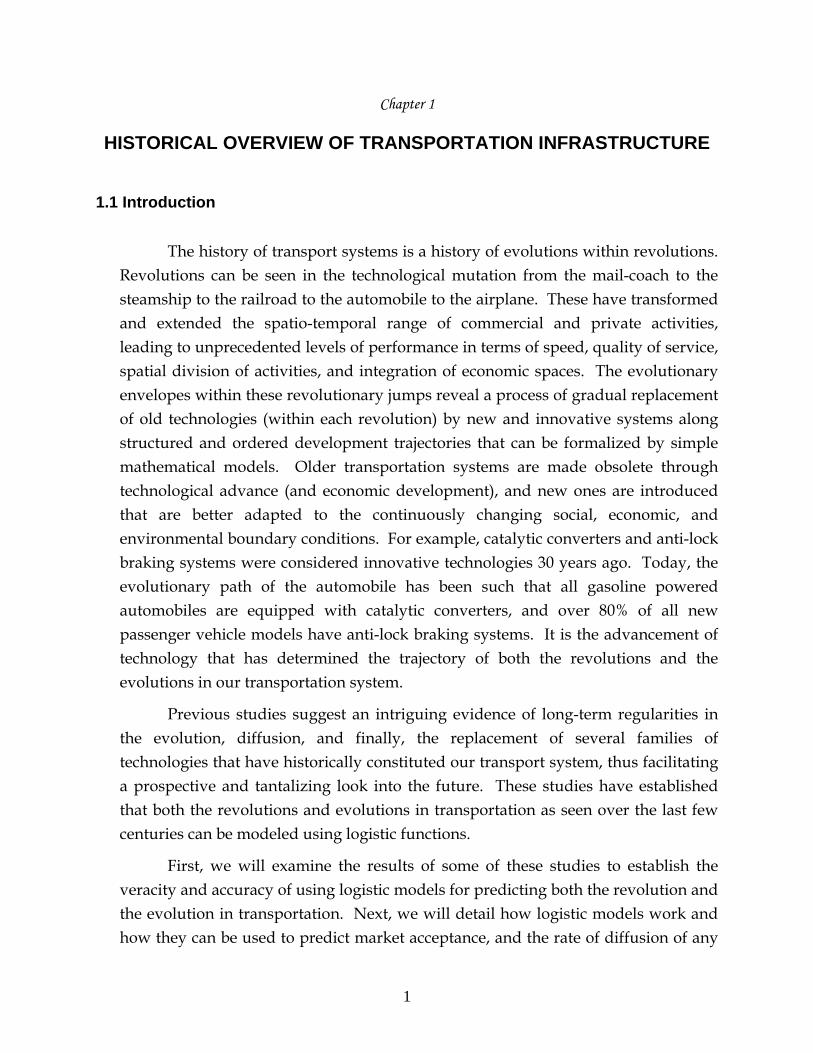
It is natural to assume that as the population increases, so does the number of
drivers. Data also suggests that the increase in driving is faster than the increase in
population, indicating that other factors besides population contribute to congestion.
The following graphs illustrate this phenomenon.
0
5
10
15
20
25
30
35
Population Miles of Highway
Perc
enta
ge C
hang
e (1
982
to 1
997)
22 %
33 %
Figure 2.3 Percent change in population and percent increase in the miles of
highways constructed, (Data source: BTS)
The graph in Figure 2.3 shows the percentage change in population and
percentage change in highway lane miles. The graph indicates that while there was a
22% increase in population from 1982 to 1987, there was a 33% increase in highway
miles. This indicates that the amount of highway construction during the said period
was growing more rapidly than population.
16

250
Figure 2.4 Population growth and increase in population in major cities in
Texas, (Data source: TxDOT)
Figure 2.4 compares the percentage change in population with percentage
change in vehicle miles traveled (VMT) in some of the major cities in Texas. All
across the state, the percentage of change in VMT is at least double that of the
change in population. Reasons for that phenomenon may be found in Figure 2.5.
0
50
100
150
200
Houston Dallas Austin Fort Worth SanAntonio
El Paso Laredo CorpusChristi
Perc
enta
ge C
hang
e (1
982
to 1
997)
% Change in Population % Change in Vehicle Miles Traveled
17

Increase in Trip Lengths
35%
Increase in Trips Taken
18%
Decrease in Vehicle
Occupancy17%
Switch to Driving17%
Increase in Population
13%
Figure 2.5 Factors for increase in driving, (Data source: BTS)
Figure 2.5 depicts the relative weights of the various factors that are responsible
for the increase in driving. This U. S. Bureau of Transportation Statistics (BTS) data
dispels the population myth, pointing out that an increase in population is the least
factor for the growth in driving. An increase in trip lengths is the greatest reason for the
growth in driving. Other factors include an increase in the number of trips taken, a
decrease in vehicle occupancy, and a number of people switching from other modes of
transportation to driving.
Part of the reason for the increase in driving and the decrease in vehicle
occupancy has to do with the nature of households. There are more licensed drivers
per household today than ever before. At the same time, these drivers are more
likely to have their own cars than drivers of the past. Figure 2.6 illustrates this situation
of American drivers.
18

2.0
Licensed Drivers per Household1.6
Vehicles per Licensed Driver1.2
Num
ber
Vehicles per Capita (TX) 0.8
Vehicles per Capita (US) 0.4
0.0 1960 1970 1980 20102000 1940 1950 1990
Year
Figure 2.6 Vehicles and licensed driver ratios, (Data source: BTS)
2.3 Number of Registered Vehicles
Figure 2.6 shows the vehicles per capita in Texas and the U.S., number of vehicles
per licensed driver and number of licensed drivers per household from 1950 forward.
As the graph illustrates, the vehicles per capita in the U.S. is currently around 0.8, more
than twice the amount of that in 1950. Licensed drivers per household have also
increased, with an average of 1.8 per household. In Texas, the vehicles per capita is
about 0.6. Due to more licensed drivers per household and the increasing vehicles per
capita, there will be more vehicles on the highways.
19

0
50
100
150
200
250
300
350
1950 1960 1970 1980 1990 2000 2010 2020Year
Vehi
cles
Reg
iste
red
(Mill
ions
)
Figure 2.7 Total vehicles registered in the U.S., (Data source: BTS)
Figure 2.7 shows the number of vehicles registered in the U.S. (in millions) as a
time series. As the graph indicates, currently, there are about 220 million registered
vehicles in the United States. By the year 2020, there will be more than 300 million.
The number of registered vehicles are increasing as a result of increases in vehicles per
capita as well as the growth in the number of licensed drivers.
20

16
Figure 2.8 Vehicles registered in Texas vs. time, (Data source: TxDOT)
Figure 2.8 shows the number of vehicles registered in Texas from 1915 to 2000.
Also the number of trucks and autos registered has been separated. Currently, there
are approximately 14 million vehicles registered in Texas. Both the number of
automobiles and trucks are growing. The distinction between trucks and
automobiles is necessary if one is to fully grasp the impact that vehicles are having
on the roads. Truck traffic is more detrimental to the pavement than automobile
traffic. One pass of an 18-kip ESAL (Equivalent single axle load) is equivalent to 5,000
passes of a passenger car.
0
2
4
6
8
10
12
Vehi
cles
Reg
iste
red
(Mill
ion)
14
Autos and Trucks
Autos
Trucks 19
30
1935
1940
1945
1950
1955
1960
1965
1990
1995
2000
1925
1920
1970
1975
1980
1985
1900
1905
1910
1915
Years
21

0
15
30
45
60
75
90
El-Paso Austin San-Antonio
Dallas Houston
Mile
s Tr
avel
led
(Tho
usan
ds)
19821997
Figure 2.9 Vehicle miles traveled in major cities in Texas, (Data Source: TxDOT)
Figure 2.9 shows the increase in the vehicle miles traveled form 1982 to 1997 in
some of the major cities in Texas. As the graph illustrates, five major cities in Texas
witnessed a tremendous increase in vehicle miles traveled between 1982 and 1997.
150160170180190200210220230240250
Jan-92 Jan-94 Jan-96 Jan-98 Jan-00 Jan-02
Year
Bill
ions
of M
iles
Underlying trend
Figure 2.10 Vehicle miles traveled in Texas vs. time, (Data source: BTS)
22

Figure 2.10 shows the VMT in the U.S. from 1992 to 2002. The estimate for
January, 2002 shows 220 billion vehicle miles traveled on the U.S. highways. This
amount is a 30 billion point increase over the estimate of 1993. For the most part, the
increase in vehicles miles traveled has remained steady. In order to get a clearer
vision of the areas most seriously affected, figure 2.11 breaks this trend up into urban
and rural sectors.
4 3.5
Total 3
VMT
(Tril
lions
)
2.5 Urban2
1.5 Rural1
0.5 0 1950 1960 1970 1980 1990 2000 2010 2020 2030
Year
Figure 2.11 Vehicle miles traveled in urban and rural areas in the U.S. vs. time,
(Data source: BTS)
As figure 2.11 illustrates, the urban sector is witnessing a much greater
increase in vehicles miles traveled than the rural sector. Figure 2.12 illustrates the
increase of VMPT for trucks.
23

350
300
250
VMT
(Bill
ions
)
200
150
100
50
0 1960 1970 2020 1980 1990 2000 2010 2030
Year
Figure 2.12 Vehicle miles traveled by the trucks in the U.S. vs. time, (Data source: BTS)
100
80 Automobiles
Perc
ent o
f VM
T 60
40
Trucks 20
0 1965 1970 1975 1980 1985 1990 1995 2000 2005
Year
Figure 2.13 Percentage of VMT for autos and trucks, (Data source: BTS)
Figure 2.13 indicates the proportion of VMT by Automobiles and Trucks from
1970 to 2000. Trucks traveled about 200 billion miles in 2000, making up 40 % of the
total vehicle miles traveled. While the percentage of automobiles is higher than the
percentage of trucks, the percentage of automobile VMT is decreasing while the
24

percentage of truck VMT is increasing. Looking towards the future, the percentage
of vehicle miles traveled by trucks could increase by more than 400% by the year
2020.
4500
3750
Ton
mile
s (B
illio
ns)
3000
2250
1500
750
0 1950 1960 1970 1980 1990 2000
Year
Figure 2.14 Ton-miles of freight carried vs. time, (Data source: BTS)
Figure 2.14 illustrates the increasing ton-miles of freight transportation. In the
last forty years, the ton miles of freight have increased by over 50%. This trend
promises to keep growing in the future.
Figure 2.15 breaks down the ton miles of freight into three different methods of
transportation: rail, truck, and water.
25

1,500
Class 1 Rail 1,200
Ton
Mile
s of
Fre
ight
Intercity Trucking
900
(
Bill
ions
)
Water600
300
0 1950 1960 1970 1980 1990 2000
Year
Figure 2.15 Modes of transportation for ton miles of freight carried vs. time,
(Data source: BTS)
While barge/ships are the cheapest means of transporting freight, it is used
much less frequently than rail or intercity trucking because it is relatively slow, and
limited in the regions it can serve. Intercity trucking is currently behind first class
rail transportation; however, trucks are catching up quickly.
Comparing the percentages of the U.S. NAFTA trade and various modes (truck,
rail, pipeline, air, water, etc) used for transportation shows that trucks are the major
carriers of freight both in terms of value and weight. Figure 2.16 illustrates this statistic
for Texas roadways.
26

70 VALUE WEIGHT
60
50
PER
CEN
T
40
30
20
10
0 Truck Rail Pipeline Air Water Other and
Unknown
Figure 2.16 Percentage of NAFTA freight transported in Texas by various modes,
(Data source: BTS)
Figure 2.16 shows the percentage of freight transported through various modes
of transportation in Texas. The graph shows, that Texas relies a great deal more on
trucks to transport freight than any other mode of transportation.
27

2.4 The Congestion Index
While all of these statistics on vehicles illustrate the growing trend in traffic
congestion, it is helpful to analyze the congestion index as well. The following
charts illustrate the congestion index for a variety of cities in Texas.
0.5
0.6
0.7
0.8
0.9
1.0
1.1
1.2
1980 1985 1990 1995 2000Year
Con
gest
ion
Inde
x
Houston
DallasAustinFortworth
San Antonio
Figure 2.17(A) Congestion index for major cities in Texas, (Data source: TTI)
1.0
0.9 Beaumont
Con
gest
ion
Inde
x
0.8
Corpus Christi Brownsville0.7
0.6 Laredo
0.5
0.4 1980 1982 1984 1994 1996 1986 1988 1990 1992 1998
Year
Figure 2.17(B) Congestion index for major cities in Texas, (Data source: TTI)
28
Figures 2.17(A) and 2.17(B) indicate the congestion index for some cities in Texas
from 1982 to 1997. The congestion index is the ratio of the travel demand to the capacity
of roadways during peak periods. From 1982 to 1993, most of the metro cities first
show an increase and then a decrease in the congestion index. However, the years
between 1995 and 1997 witnessed a constant increase in the roadway congestion
index. An index value greater than 1.0 indicates problematic congestion. While
Brownsville, Corpus Christi, and Laredo appeared to be less than 1 in 1997,
Beaumont's index ran dangerously close to 1.0. A look at the other graph reveals
that Dallas, Austin, and Houston were already in the danger zone in 1997. Fort
Worth and San Antonio were each at an index of .9, slowly approaching 1.0.
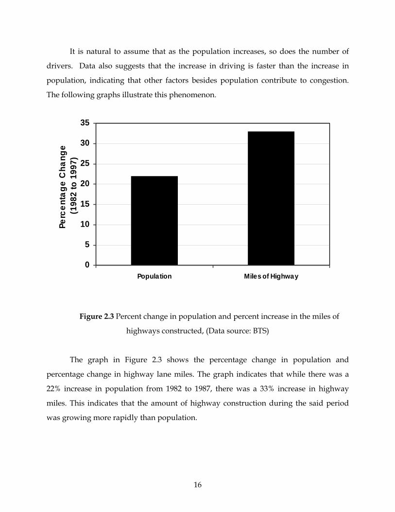
2.5 Consequences of Congestion
Congestion wastes time, energy, and money. Figure 2.18 illustrates the average
time it takes drivers to travel to work in the United States.
17
20
23
26
29
1970 1980 1990 2000 2010 2020 2030Year
Trav
el T
ime
(Min
s)
Figure 2.18 Average travel time to work in the U.S. (Data Source: BTS)
29

Over the last two decades, the average travel time to work in the U.S. has
increased from 22 minutes to 24 minutes. If we project this rate into the future, the
average time could increase to 27 minutes by 2020.
1.2 Houston
1.1 Dallas
1.0 Fort Worth Austin
0.9
Con
gest
ion
Inde
x
0.8 San Antonio
0.7
0.6
0.5 1980 1985 1990 1995 2000
Year
Figure 2.19 Fuel wasted due to congestion vs. time, (Data source: TTI)
Figure 2.19 shows millions of gallons of fuel wasted due to congestion from 1982
to 1997. According to this graph Dallas, Fort Worth, San Antonio, Austin, and El
Paso have all witnessed a significant increase in the amount of fuel wasted due to
congestion. Dallas has shown the highest increase in the amount of fuel wasted,
going from 30 million gallons wasted in 1982 to 165 million gallons wasted in 1997.
San Antonio went from wasting 15 million gallons in 1982 to 60 million gallons in
1997. Austin and Fort Worth followed similar trends. El Paso witnessed the
smallest increase in wasted fuel.
30

Wasting fuel and time in traffic raises a variety of concerns. One concern is large
amount of money lost annually. Figure 2.20 illustrates the annual congestion cost per
driver in major Texas cities. The graph takes into consideration both the wasting of fuel
and time.
12
1996 1997 1994
Cos
t per
Driv
er ($
Hun
dred
s)
10
8
6
4
2
0 Houston Austin Laredo CorpusSan
Antonio Christi
Figure 2.20 Congestion cost per driver in Texas, (Data source: TTI)
The cost of congestion is felt in other areas as well. As congestion increases, so
does the cost of truck freight and service operations. These costs have negative impacts
on the manufacturing industry and the service sector, and are passed on to the
consumers.
31

2.6 Fuel Consumption
Of course, an increase in gasoline prices is not just due to the amount of fuel that
is wasted because of congestion. Gas prices rise as fuel becomes scarcer and
more difficult to access. As the U.S. does not produce enough petroleum to rely on
its own resources for consumption, fuel must be purchased from foreign countries. The
following graph illustrates this problem.
Figure 2.21 Petroleum production and consumption in the U.S., (Data source: DOT)
As shown in Figure 2.21, the U.S. consumption of petroleum far exceeds its
production, with the transportation sector consuming a great percentage of the
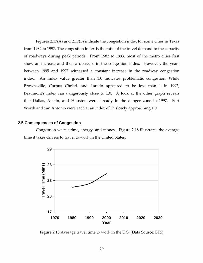
petroleum consumed. Figure 2.22 specifically looks at the amount of energy that is
consumed by the transportation sector alone each year in the U.S.
32
70
60
Tota
l Ene
rgy
Con
sum
ed
50
40
(Tril
lion
BTU
)
30
20
10
0 1955 1965 1975 1985 1995 2005
Year
Figure 2.22 Total energy consumed by transportation sector,
(Data source: DOE)
Figure 2.22 illustrates the total energy consumed by the transportation sector
from 1960 forward. The transportation industry’s yearly consumption of energy
resources has increased significantly since the 1960’s.
Figure 2.23 demonstrates the domestic demand for gasoline by mode of
transportation, breaking up transportation into categories of "highway" and
"non-highway."
33

0
100
200
300
400
500
1955
1960
1965
1970
1975
1980
1985
1990
1995
2000
Year
Gas
olin
e (B
illio
n lit
ers)
Non-highway
Highway
Figure 2.23 Domestic demand for gasoline by mode of transportation,
(Data source: BTS)
According to the graph, the demand for gasoline by highway modes of
transportation increased linearly from 1960 to 1975. After that time, the increase was
slower. Between 1990 and 1992, the demand for gasoline by highway modes of
transportation dropped but since 1992, the demand for gasoline by highway modes of
transportation has increased linearly. By contrast, the demand for gasoline by
non-highway modes of transportation has remained almost constant since 1960,
decreasing by just a minimal amount. The overall demand for gasoline by non-
highway modes of transportation is significantly less than the overall demand for
gasoline by highway modes of transportation.
34

Figure 2.24 breaks down the energy consumption of the highway modes of
transportation into two categories: 1) Autos and light vehicles, and 2) Buses and trucks.
0
4,000
8,000
12,000
16,000
20,000
1965 1970 1975 1980 1985 1990 1995 2000 2005Year
BTU
(Tril
lion)
Autos and Light
Buses and Trucks
Figure 2.24 Total energy consumption, (Data source: BTS)
The demand for gasoline has been somewhat erratic for autos and light
vehicles, but there has been an overall increase in consumption. Buses and trucks
however, have witnessed a steadier increase over time.
35
Fuel
Con
sum
ed p
er V
ehic
le (H
undr
ed
10
8 G
allo
ns) 6
4
2
0 1955 1960 1990 1995 1965 1970 1975 1980 1985 2000
Year
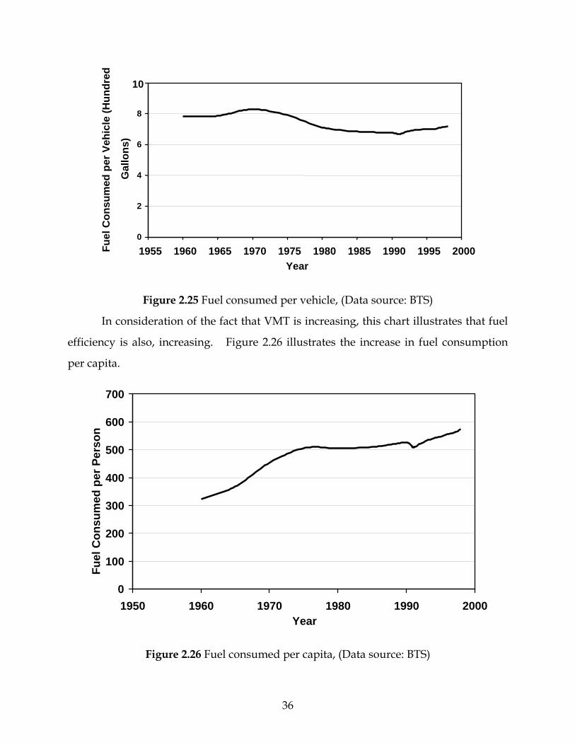
Figure 2.25 Fuel consumed per vehicle, (Data source: BTS)
In consideration of the fact that VMT is increasing, this chart illustrates that fuel
efficiency is also, increasing. Figure 2.26 illustrates the increase in fuel consumption
per capita.
700
600
Fuel
Con
sum
ed p
er P
erso
n
500
400
300
200
100
0 1950 1960 1970 1980 1990 2000
Year
Figure 2.26 Fuel consumed per capita, (Data source: BTS)
36

35
5
1
1
2
2
3Fu
el C
onsu
med
(Bill
ion
gallo
ns) 0
5
0
5
0
0 1965 1970 1975 1980 1985 1990 1995 2000
Year
Figure 2.27 Fuel consumed by trucks, (Data source: BTS)
As shown in Figure 2.27, from 1970 to 2000, the trucking industry has witnessed
an almost a 270% increase in fuel consumption.
25
Passenger Cars
20 Vans
VMT per Gallon 15
Mile
s
10 Trucks
5
0
1970 1975 1995 1980 1985 1990 2000
Year
Figure 2.28 Miles traveled per gallon, (Data source: BTS)
37

Figure 2.8 illustrates that while trucks are witnessing a rise in their consumption
of fuel, they are not experiencing an increase in miles traveled per gallon of fuel. Unlike
other vehicles, their fuel efficiency is not increasing.
2.7 Alternate Fuel Vehicles
Vehicles of this type offer a way for consumers to do their part in alleviating
energy related problems in the U.S. Figure 2.29 illustrates the number of alternate fuel
vehicles sold throughout the U.S.
Figure 2.29 Alternate fuel vehicles sold in Texas, (Data source: BTS)
Figure 2.29 shows the number of Alternative vehicles sold in the US from 1992
onwards. From 1992 to 1993, there was an initial surge in the market for alternate
fuel vehicles. Since 1993, the purchase of alternate fuel vehicles has risen gradually.
Vehicles using alternate fuel touched a figure of around 450,000 by year 2001.
1
2
3
3
4
Num
ber o
f Ve
hicl
es (T
hous
ands
) 525
50
75
00
25
50
75
0 1990 1992 1994 1996 1998 2000 2002
Year
38

A variety of drivers seek out alternate fuel vehicles. Figure 2.30 illustrates the
different types of vehicles that are using alternate fuel.
Light Duty Trucks50%
Vans28%
Others1%
Automobiles21%
Figure 2.30 Alternate fuel consumption by various modes of transportation,
(Data source: BTS)
As the pie chart indicates, 50% of alternate fuel vehicles are light duty trucks.
The next major users are vans at 28%. Automobiles follow with 21%.
39

Figure 2.31 Alternate fuel vehicles purchased per state,
(Data source: DOE)
California is the leader in the market of alternate fuel vehicles with Texas
following close behind. However, these statistics change somewhat when the number
of alternate fuel vehicles is normalized with the population of each state. When this is
considered, as shown in Figure 2.31, Nebraska comes in highest followed by Indiana
and Oklahoma.
Alternate fuel vehicles employ a variety of different resources that take the place of
petroleum. The following graph gives us an idea of the different kinds of resources
being used and suggests the popularity of each.
0
1
2
3
4
5
6
7
Vehi
cles
Per
100
0 Pe
rson
s
USA
O
HIO
TEXA
S
CA
LIFO
RN
IA
G
EOR
GIA
FLO
RID
A
IN
DIA
NA
N
EBR
ASK
A
OK
LAH
OM
A
PE
NN
SYLV
AN
IA
MIC
HIG
AN
NEW
YO
RK
40
LPG CNG M85 E85 Electricity1,000,000 Fu
el C
onsu
med
, tho
usan
d G
asol
ine
100,000
Equi
vale
nt g
allo
ns
10,000
1,000
100
10
1 1992 1995 1998 1999 2000 2001
Year
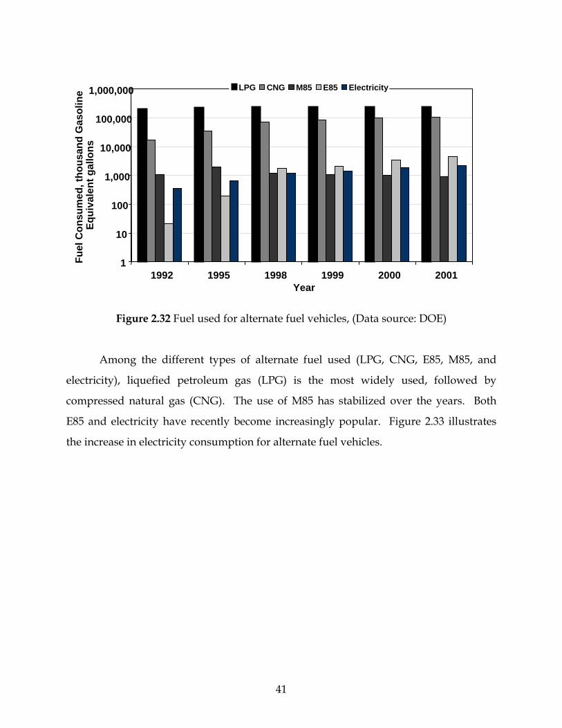
Figure 2.32 Fuel used for alternate fuel vehicles, (Data source: DOE)
Among the different types of alternate fuel used (LPG, CNG, E85, M85, and
electricity), liquefied petroleum gas (LPG) is the most widely used, followed by
compressed natural gas (CNG). The use of M85 has stabilized over the years. Both
E85 and electricity have recently become increasingly popular. Figure 2.33 illustrates
the increase in electricity consumption for alternate fuel vehicles.
41

0
500
1000
1500
2000
2500
1990 1992 1994 1996 1998 2000 2002Year
Elec
tric
ity C
onsu
mpt
ion
(100
0 G
allo
ns G
asol
ine
Equi
vale
nt)
Figure 2.33 Electricity consumption by alternate fuel vehicles,
(Data source: DOE)
Figure 2.33 shows the amount electricity consumed (in gasoline equivalent
gallons) in the U.S. As the graph indicates, the alternate fuel vehicle market has
witnessed a tremendous increase in the use of electricity. From 1992 to 2001 the
consumption of electricity for alternate fuel vehicles quadrupled.
42

Figure 2.34 Money spent on transportation, (Data Source: TX DOT)
Figure 2.34 illustrates the percentage of money the state of Texas has allocated to
the transportation sector since 1918. A major percentage of money was spent on
the transportation sector when the interstate issue was being built. Since then, a
negligent attitude has been shown towards the transportation sector. Funds allotted
for the transportation sector reached an all time low in 1997 of 7%.
When the Texas initially increased its spending in the transportation sector, it
raised gasoline tax rates to balance the increase. However, as the gasoline tax rate has
remained the stagnant for a long time. Figure 2.35 illustrates this situation and also
compares the rates of Texas with averaged rates of other states.
43
0
5
10
15
20
25
1985
1986
1987
1988
1989
1990
1991
1992
1993
1994
1995
1996
1997
1998
1999
2000
Year
Tax
Rat
e (c
ents
/gal
lon)
FOR TEXAS STATE AVERAGE
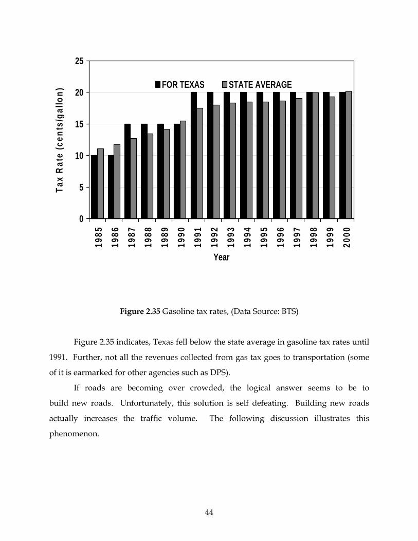
Figure 2.35 Gasoline tax rates, (Data Source: BTS)
Figure 2.35 indicates, Texas fell below the state average in gasoline tax rates until
1991. Further, not all the revenues collected from gas tax goes to transportation (some
of it is earmarked for other agencies such as DPS).
If roads are becoming over crowded, the logical answer seems to be to
build new roads. Unfortunately, this solution is self defeating. Building new roads
actually increases the traffic volume. The following discussion illustrates this
phenomenon.
44

Figure 2.36 Travel rate index, (Data Source: TTI)
Figure 2.36 shows the Travel Rate Index from 1982 to 1997 for two cases – high
road building areas and low road building areas.
As this chart indicates1, the high road-building areas increased road capacity
per person by 28%, while the low-road building areas actually decreased road
capacity per person by 11%. However, the high road building areas witnessed
higher congestion levels than the low road-building areas. Both groups experienced
congestion during rush hour traffic at about the same levels.
People are attracted to new roads. When new roads are built, people who
would generally avoid driving during high congestion times suddenly take to their
vehicles. Others join the new roads hoping to save time. Over a period of time,
congestion increases.
1 This chart, and the information accompanying it in this paragraph and the next, can be found in a report published by The Surface Transportation Policy Project at http://www.transact.org/Reports/constr99/sheetiv.htm
45

Despite the self defeating efforts of construction, the drive for building new
roads continues to grow. Figure 2.37 illustrates how much money is spent on
constructing new roads and maintaining old ones in Texas.
0.0
0.5
1.0
1.5
2.0
2.5
3.0
3.5
4.0
1990 1992 1994 1996 1998 2000 2002Year
Dol
lars
(Bill
ions
) Construction
Maintenance
Figure 2.37 Road construction and maintenance in Texas, (Data Source: TX DOT)
According to this graph, Texas spent almost 3.5 billion dollars in the year
2000 on road construction. The amount spent on maintaining roads, however,
seems to be decreasing.
2.8 Conclusion
While the current rate of diffusion of alternate fuel vehicles (or hybrids) as a
mode of transportation is extremely slow (these vehicles account for a fraction of a
percent of the total number of vehicles on the road), there are other factors that could
accelerate the rate of their acceptance with the consumer ‐ the most important of which
is the price of gasoline.
46

After studying the global production and consumption patterns of oil, Campbell
and Laherrere (1998), two analysts with the oil industry, arrived at a startling
conclusions. Their extensive analysis effectively debunks alarmist theories that we are
about to run out of oil. Their data suggests that the world is not running out of oil ‐ at
least not yet. But they also conclude that the end of the abundant and cheap oil on
which all industrial nations depend is near. They estimate that the switch from growth
to decline in oil production will happen within the next decade. Meanwhile, global
demand will continue to rise at more than 2% annually. Their somber conclusion:
The world could thus see radical increases in oil prices. That alone might be sufficient to curb demand, flattening production for perhaps 10 years. (Demand fell more than 10 percent after the 1979 shock and took 17 years to recover.) But by 2010 or so, many Middle Eastern nations will themselves be past the midpoint. World production will then have to fall.
These trends in the transportation industry indicate that driving is increasing
throughout the U.S. Factors for the increase in driving are varied. However, the result
is an increase in congestion, and a waste in fuel, time, and money. Texans appear to be
seeking ways to alleviate the problems associated with fuel wastage by purchasing
alternate fuel vehicles. Alternate fuel vehicles may continue to grow in popularity in
the future.
47

Chapter – 3
SURVEY OF TECHNOLOGIES In this chapter we explore some of the innovative technologies that may
shape the next major transition in transportation.
3.1 Automated Highway and Vehicle Systems
Introduction
Traffic congestion is becoming a major problem in the United States.
Frustrations associated with congestion and concerns about safety, convenience,
and pollution accelerate with the traffic. Automated Highway Systems (AHS)
provide answers to the problems associated with highway congestion by
warning passengers of possible traffic problems, coordinating traffic signals
within a community, and providing information that will increase the response
time of emergency vehicles. AHS has the potential to increase driver and
passenger safety, increase capacity, and reduce congestion. A variety of systems
and technologies exist under the general category of AHS. In this section, we
will provide a brief overview of some of these systems as well as discuss some of
the related technologies such as hands-off driving and adaptive cruise control.
A. Intelligent Transportation Systems
The U.S. Department of Transportation states that Intelligent
Transportation Systems, or ITS, should "promote the implementation of a
technically integrated and jurisdictionally coordinated transportation systems
across the county."1 The following is a list of systems that could enhance the low
of traffic and improve communication throughout the transportation sector.2
1 "Intelligent Transportation Systems." 22 June 2002. <http://www.iowaontrack.com/questions.htm> 2 The following summarizes the information provided by ITS Deployment Tracking at <http://itsdeployment2.ed.ornl.gov/its2000/definitsions.asp>
48

1. Freeway Management Systems: Freeway Management Systems employ
personnel in Freeway Management Centers to electronically monitor traffic
conditions. Through a variety of technologies, including Variable Message
Signs, Highway Advisory Radio, and In-Vehicle Signing, their personnel have
the ability to provide travelers with information to help them avoid congestion.
2. Incident Management Systems: Incident Management Systems specifically
target problems such as collisions, disabled vehicles, and debris. When operators
become aware of a problem impeding traffic, the appropriate response agency is
alerted and provided with the best route possible to the site to remedy the
situation and redirect the traffic.
3. Traffic Signal Control: With the help of Traffic Signal Control, traffic can be
coordinated along urban arterials, networks, and the Central Business District.
Traffic Signal Control adjusts the amount of green light time per street based on
either historical traffic conditions or real time emergencies.
4. Regional Multimodal Traveler Information Systems: These information
systems collect real time traffic information and make it available to travelers to
allow them to plan their routes accordingly. A variety of technologies including
broadcast radio, the Internet, and cable TV make this information accessible.
5. Transit Management Systems: Transit Management Systems electronically
monitor transit vehicles to check the actual location of the vehicle against its
scheduled location. If a transit vehicle is behind schedule, measures can then be
taken to alert potential travelers and suggest an adjusted route for the transit
vehicle. This system will also be helpful in emergency and maintenance
situations that involve transit vehicles.
49

6. Electronic Toll Collection: In Electronic Toll Collection, roadside technology
identifies a particular vehicle and charges its driver's toll account accordingly.
This system could reduce traffic delay at toll collection plazas, reduce the need
for drivers and public agencies to handle money, and reduce toll agency costs. A
common payment media would need to be established between collecting
agencies.
7. Electronic Fare Payment: Electronic Fare Payment allows travelers to
electronically pay for travel related fares and parking fees. This technology
eliminates the need for both travelers and public agencies to handle the money
required for these transactions.
8. Highway Rail Intersections: Automated systems can be employed to better
coordinate traffic control signal systems with rail movements. Roadway
travelers can be alerted in advance of the timing of railway crossing closures.
These systems may also improve the warnings that are already given at
highway-rail intersections.
9. Emergency Management: Emergency Management Services monitor
emergency vehicle traffic patterns, apprising drivers of the best route possible.
With this system, both emergency notification and response time can be
improved.
The implementation of any or all of these systems could lead to a more
efficient, less congested, and safer driving experience.
50

B. Hands-Off Driving3
Hands-off driving allows drivers to take on the roles of passengers for
most of their driving experiences. With this technology, cars can travel
independently of their driver's manipulation for most of the ride. They can
change lanes, accelerate, and decelerate in order to adjust to surrounding traffic
conditions. This technology can be implemented in a variety of ways. The two
most probable approaches involve cameras and magnets.
In the camera system, cars are equipped with small television cameras, a
computer, and vehicle-control actuators. All these devices work together to
maneuver the vehicle and keep it within the lane markings. Hands-off driving
can easily be implemented with this system as the only technological changes
that need to be made within the highway system are inside the cars themselves.
In contrast, the system that employs magnets would require structural
changes on the actual highway. In a magnet-based system, vehicles are kept in
place by magnets that are embedded along the center of the lane. Magnets are
placed 1.2 centimeters apart, and the vehicles can stay on track with less than 7.5
centimeters of error. The cost of magnet implementation would be about $10,000
per lane mile. While this technology may seem expensive, it is much cheaper
than the cost of building new lanes, which is estimated at $1 million per lane-
mile.
The benefits to hands-off driving are four fold, providing answers for
concerns about safety, traffic congestion, pollution, and economics. In the United
States, 40,000 people are killed and 5 million people are injured each year in
automobile crashes. Ninety percent of these crashes are the result of human
error. Hands-off driving could significantly reduce the number of accidents that
are a result of human error.
3 All of the information on hands-off driving comes from Bob Bryant's article "Actual Hands-off Steering: And Other Wonders of the Modern World" published in Public Roads Online. The information can be accessed at <http://www.tfhrc.gov/pubrds/pr97-12/p32.htm>
51

Reducing the number of accidents would save lives and money. The cost
of auto accidents is about $150 billion each year. The cost of congestion can be
estimated at about $50 billion each year. By reducing the number of accidents
and the amount of congestion on highways, hands-off driving could save a
significant amount of money.
Safely decreasing the space between vehicles on the highway from one
vehicle length to half a vehicle length, thereby doubling or even tripling highway
capacity could alleviate congestion. As congestion often results in accidents, this
would also promote safety.
As congestion decreases, so would pollution. Vehicles that move together
in a tight automated platoon have a dramatic reduction in aerodynamic drag that
could reduce tail-pipe emissions by 20 to 25 %.
Hands-off driving was successfully tested recently. In 1997, the National
Automated Highway System (NAHSC) demonstrated hands-off driving and
other intelligent transportation technologies in San Diego. The demonstration
was successful, and 98% of the riders said they believed the technologies could
improve highway safety, while 87% felt that the technologies could reduce
congestion on highways. Companies that participated in the demonstration
include Eaton Vorad, Houston Metro, Honda, The Ohio State University
Transportation Research Center, and Toyota.
52

Figure 3.1 Adaptive Cruise Control
C. Adaptive Cruise Control
While the technology used in hands-off driving may seem somewhat alien
to our current means of operating vehicles, another technology exists that is not
so difficult to imagine. Adaptive cruise control, or ACC, is an extension of the
existing cruise control feature found in most cars. While cruise control helps the
driver maintain a consistent speed, ACC helps the driver to adjust to the speed of
the car in front. The system controls the accelerator, engine power train, and
vehicle brakes to maintain a desired time (or distance) gap between the vehicle
ahead. Figure 3.1 (above) is a picture of adaptive cruise control.
The ACC system is equipped with a microwave radar (or a laser) unit to
monitor the vehicle ahead of it. The radar or laser reads the distance and speed
of the vehicle ahead, and a computer adjusts the car's movements to match. The
driver of the car can override ACC at any time simply by braking. Figure 3.2
illustrates the mechanics of such a radar system.
53

Figure 3.2 A schematic showing how Doppler Radar System works
Another technology that may be employed with or without ACC is CWS,
or Collision Warning System. CWS simply warns the driver through visual or
audio signs that a collision is imminent and braking and evasive steering are
needed. Currently, most commercial vehicles are equipped with CWS.4
The benefits of ACC and CWS are easy to see. Like hands-off driving,
ACC limits highway congestion. Figure 3.3 illustrates the increase in capacity
that can be achieved when ACC is employed. When cars are not equipped with
ACC, capacity of a lane is between 2200 to 2400 passenger cars per hour. With
ACC, the capacity can increase to over 3200 passenger cars per hour per lane.
4 "Beyond Cruise Control." The Economist 359.8227 (2001): 33-37.
54

INCREASE IN CAPACITY
14800
7500
49003700
0
2000
4000
6000
8000
10000
12000
14000
16000
25 50 75 100
Headway ( in Feet )
pcpl
ph
Figure 3.3 Increase in capacity due to Adaptive Cruise Control
Like hands-off driving, CWS could reduce the number of accidents per
year. By warning the driver of potential problems, CWS reduces the accidents
that result from human errors, such as being distracted or falling asleep.
Adaptive Cruise Control has been successfully tested in a recent
demonstration project. A hundred drivers were instructed to use the ACC
feature installed in Chrysler Concorde Sedan vehicles in their natural driving
environment. Some drivers tested the technology for two weeks; others tested it
for five weeks. Surveys were conducted after the project, and the results
indicated that drivers would not use ACC in dense traffic conditions. However,
when traveling above 35 mph, drivers used ACC for about half of the distance
traveled.
55

Currently, the USDOT, General Motors, and Delphi Automotive Systems
are collaborating on a five year, $35 million research project that will design and
test a fleet of ten high powered vehicles equipped with high-tech collision
warning systems.5
Companies involved with ACC include TRW Automotive Electronics,
Delphi Delco Electronics, Bosch, Daimler Chrysler, and Haldex Brake Systems.
Eaton Vorad Technologies are currently experimenting with CWS. On average,
the cost of implementing ACC and CWS is $2000-$3000 per vehicle.
Conclusion
The implementation of any or all automated highway systems could
drastically improve the condition of today's highways. With ITS, ACC, CWS,
and hands-off driving, roads could become safer and more efficient. Congestion
and pollution could significantly be reduced. Automated Highway Systems
offer exciting possibilities for the future of transportation.
3.2 Alternate-Fueled Vehicles Introduction
The transportation industry in the United States faces a challenge in the
use of energy resources. Petroleum, the traditional fuel used, is an exhaustible
resource that is liable to increase in price as it decreases in availability. The
transportation sector accounts for two-thirds of the total consumption of
petroleum in the U.S.
Pollution from the emissions of internal combustion engines is also a
major concern due to its negative impact on the environment and the health of
people.
These concerns with traditional Internal Combustion (IC) vehicles have
paved the way for alternative fuel vehicles. Alternative fuel vehicles employ 5 "The Ultimate in Crash Safety is Avoiding Crashes." 20 July 2000. 26 October 2001. <http://www.gm.com/cgi-bin/pr_display.pl?1510>
56

electricity (or CNG) as a source of power, rather than relying solely on gasoline.
They reduce the need for petroleum and decrease the emission of green house
gases. Electric vehicles can be organized into three categories for discussion: fuel
cell vehicles, battery powered vehicles, and hybrid electric vehicles.6
A. Fuel Cells
Fuel cell vehicles use fuel cells as electrochemical engines "that generate
electricity by harnessing the reaction of hydrogen (fuel) and oxygen (from air)
without combustion or pollution. The only byproducts are water and heat."7
Even when fuel cell vehicles use gasoline, they use it more efficiently than
traditional IC vehicles, providing economic as well as environmental benefits.
Internal combustion engines only use about 19% of the energy in gasoline; fuel
cell vehicles can more than double that efficiency.
Fuel cell vehicles are currently being developed world wide by major auto
manufacturers. Both the United States and Canada have been running
demonstrations of fuel cell technology with buses that run on fuel cell engines.
Specifically within the United States, California has been testing fuel cell vehicles
since the year 2000. Fuel cell vehicles may become a popular alternative for both
public and personal transportation in the future.
B. Battery Electric Vehicles
Battery-electric vehicles run entirely on electricity from batteries. Rather
than being refueled, battery-electric vehicles are recharged. Batteries may be
recharged at home or at charging stations that can be found in a variety of states
across the U.S. including California, Arizona, Massachusetts, Florida, Vermont,
North Carolina, South Carolina, and Texas.
6 All of the information presented on alternate fuel vehicles can be found online at <http://www.yournextcar.org>. 7 Your Next Car. 26 June 2002 <http://www.yournextcar.org/fuelcells.html>.
57

The power gained in one charging session varies according to the
technology employed. Charging sessions can be analyzed at three different
levels. At the most basic level, charging can be done in twelve to sixteen hours
with a standard, grounded 120V, 3-prong outlet that is available in most homes.
The next level of charging requires eight to ten hours and a 240V, 40amp
charging. The third level of technology currently being developed will require
480V to provide a complete recharge in just fifteen minutes.
The life cycle of a battery and the range of travel it provides will depend
on the type of battery used. Electric vehicles may use modified versions of the
lead acid batteries that are used in traditional automobiles. Lead acid batteries
that cost about $3,000 last for three years and are reliable; however, vehicles
powered by these kinds of batteries may only travel a range of less than 100
miles before they need to be recharged. Nickel-Cadmium batteries and Nickel-
metal hydride batteries both have a longer life cycle and provide cars with longer
ranges; however, they are initially more expensive than lead acid batteries.
Finally, lithium-ion batteries provide both an extensive range and an extensive
life cycle; however, they may have a tendency to encounter more problems when
overcharging or high charging occurs.
As battery electric vehicles are recharged, rather than refueled, they offer
environmental benefits, eliminating mobile-source emissions. However, the
benefits of battery electric vehicles extend beyond the environmental realm.
Battery electric vehicles are actually safer than fuel powered vehicles. While
battery electric vehicles do not minimize the possibility of accidents, they do
significantly reduce the possibility of a collision resulting in fire because they do
not have gas tanks or reservoirs of flammable oil.
Battery electric vehicles are being provided by a number of automobile
manufacturers including Ford, General Motors, Daimler Chrysler, Honda,
Nissan, Toyota, and Solectria. Batteries that can achieve a range of 100 miles,
making battery electric vehicles ideal for intra-city travel, power most.
58

C. Hybrids
A hybrid electric vehicle, or HEV, combines an electric motor with a
separate gasoline, diesel, or fuel cell engine. An energy storage device, such as a
battery, a flywheel, or an ultra capacitor, powers the electric motor. There are
two major types of hybrids: parallel and series. Parallel hybrids rely on the fuel
engine for their major source of power, only utilizing the electric motor in
instances that require extra power, such as climbing hills and accelerating. In
series hybrids, electricity is generated by the internal combustion engine or fuel
cell to charge the energy storage device. The electric motor alone provides the
drive train with power. Of the two types, series hybrids have lower pollution
level.
Hybrids may be more convenient than battery electric vehicles because
not all hybrids have to be plugged in to be recharged. Some hybrid vehicles
recharge their batteries every time brakes are applied (regenerative braking).
An example of a hybrid is Toyota's Prius. This car completely runs on its
battery while starting, idling, and at low speeds. After a speed of 30 mph, both
battery and gasoline are used.8 The Prius provides gas mileage of up to 50 miles
per gallon and can reach speeds up to 110 mph.
Currently, both Toyota and Honda are selling affordable hybrids. Daimler
Chrysler, Ford, General Motors, and Nissan plan to enter the hybrid sales market
in 2003 and 2004. Hybrid SUVs will even be available by Daimler Chrysler and
Ford.
Conclusion
Alternate fuel vehicles provide modifications to the traditional gasoline
powered automobile. They are economical, safe, and environmentally friendly.
As the technology of fuel cells, fly wheels, regenerative braking and other
powering devices advance, the power and range of alternative fuel vehicles will
8 This feature is specific to Toyota's Prius. Some hybrids run solely on their battery until they reach highway speeds. The technology varies vehicle to vehicle.
59

increase, and the demand for them will rise. Currently, electric vehicles may cost
any where between $18,000 and $40,000. This cost is likely to decrease as the
technology matures and mass production of the vehicle is initiated. The speed
capability of most alternate fuel vehicles is comparable to conventional gasoline
vehicles for intra-city travel. With the inevitability of change in technology in
transportation, the use of electricity for propulsion of automobiles of the future is
highly likely.
3.3 Magnetic Levitation (Maglev) Introduction
Visualize magazine may have described the future of the transportation
best when it reported, “the future of transportation may find travelers flying on
vehicles that have no wings.”9 The Maglev System makes such transportation
possible. Maglev vehicles move along a guideway, slightly levitated above the
guideway floor. The system works with a combination of magnets and electrical
coils that both propel and levitate the vehicle electromagnetically.
A. Operation
In order for a Maglev vehicle to move forward, the propulsion coils
positioned on both sides of the guideway are energized by a three-phase
alternative current from a substation. This current runs through the propulsion
coils and creates a shifting magnetic field on the guideway. The shifting
magnetic field pulls and pushes the magnets on the Maglev vehicle, moving the
vehicle forward10 as illustrated in Figure 3.4.
9 Visualize. October 2001. 13 July 2002. <http://www.technologyreview.com/articles/visualize1001.asp> 10 Principle of Maglev. 21 May 1997. 23 June 2002. <http://www.rtri.or.jp/rd/maglev/html/english/maglve_principle_E.html>.
60

Figure 3.4 Magnetic Traveling Field
(Data source: www.transrapid.de/en/index/html)
As the vehicle moves forward at a high speed, its magnets are several
centimeters below the center of the levitation coils that are positioned on both
sides of the guideway. The magnets on the moving vehicle create an electric
current within the coils that then begin to temporarily act as electromagnets.
Forces are created by this current that both push and pull the maglev vehicle
upward.11
Alternatives to this levitation system are available. One alternative lines
the guideway with the electromagnets that levitate the car: this type of system is
called an electrodynamic system. Figure 3.5 illustrates the differences:
11 Ibid.
61

Figure 3.5 Types of Levitation
(Data source: http://www.maglev2000.com/works/how.html)
In addition to levitating the vehicle, the levitation coils also ensure the
lateral guidance of the vehicle as illustrated in Figure 3.6. Levitation coils on
both sides of the guideway face each other and are connected underneath the
guideway. When the Maglev vehicle strays from the center line of the guideway,
an electric current is induced in the loop. The coils running on the guideway
nearest the vehicle are activated to repulse the vehicle, and the coils running
along the guideway on the opposite side are activated to attract the vehicle. Thus
a balance is maintained between both sides of the guideway, and the Maglev
vehicle stays centered.12
12 Ibid.
62
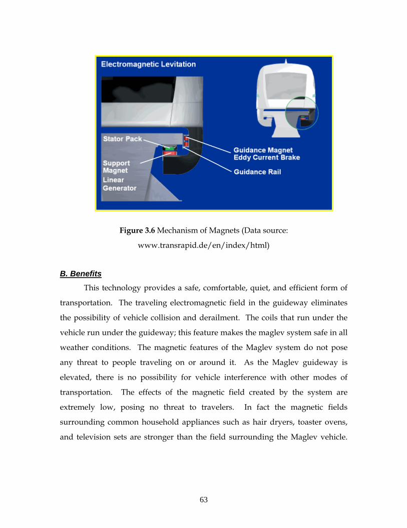
Figure 3.6 Mechanism of Magnets (Data source:
www.transrapid.de/en/index/html)
B. Benefits
This technology provides a safe, comfortable, quiet, and efficient form of
transportation. The traveling electromagnetic field in the guideway eliminates
the possibility of vehicle collision and derailment. The coils that run under the
vehicle run under the guideway; this feature makes the maglev system safe in all
weather conditions. The magnetic features of the Maglev system do not pose
any threat to people traveling on or around it. As the Maglev guideway is
elevated, there is no possibility for vehicle interference with other modes of
transportation. The effects of the magnetic field created by the system are
extremely low, posing no threat to travelers. In fact the magnetic fields
surrounding common household appliances such as hair dryers, toaster ovens,
and television sets are stronger than the field surrounding the Maglev vehicle.
63

Thus, travelers with pacemakers can travel without worry. Even credit cards
carried by the passengers will remain unaffected.13
In addition to being safe, passengers will also be comfortable. The jerking
and bumping associated in other forms of travel are eliminated with the
Maglev system. Regardless of the speed of travel, passengers riding on Maglev
vehicles have the flexibility of traveling without seatbelts. They are even free to
move about the vehicle for the duration of their trip.
The Maglev system also severely reduces the noise that is produced by
other forms of transportation. The levitation of the Maglev vehicle eliminates the
noise that is created by friction in systems of transportation where vehicle and
guideway contact are necessary. Thus, the only discernable noise generated is
wind noise. Further more, since the Maglev vehicle has a sleek aerodynamic
design, the noise it generates is considerably less than the noise generated by
high speed trains, even when the Maglev vehicle is traveling at speeds above 300
mph.14
The high speeds of Maglev travel could benefit its travelers through
convenience and economics. With the fast inter-city travel provided by Maglev,
people may live further from their jobs than they currently do. As people are
able to move further away from the city, opportunities in commercial and
residential real estate will expand. Residential prices could stabilize, and new
industries could develop in remote areas, creating new jobs. The economy
would benefit as new markets open up and perishable goods are transported
faster and cheaper via the Maglev system than via contemporary systems.15
13 The Baltimore-Washington Maglev Project. Ed. BW Maglev. 2001. <http://www.bwmaglev.com>. 14 Port Authority. Ed. Port Authority of Allegheny County. 23 June 2002. <http://www.portauthority.org/maglev/faq.html>, 15 Maglev 2000 of Florida Corporation. 23 June 2002. <http://www.maglev2000.com/works/how-08.html>.
64

As the Maglev system could provide alternatives to transport people and
fright, the demand on highways system will decline, resulting in reduced
congestion, highway maintenance costs, and mobile source of pollution. 16
When compared with other forms of transportation, the Maglev system
seems to be better on many counts. In addition to its safety features mentioned
earlier, the Maglev system has also been described as "the world's safest available
means of high-speed transport." Traveling by maglev is 20 times safer than
traveling by airplane, 250 times safer than traveling by conventional railway
systems, and 700 times safer than traveling by car.17
Maglevs are faster and potentially more economical than other rail
systems. Maglev vehicles can run up to 311 mph, while other high speed rail
systems typically reach only 185 mph. Maglev systems also posses acceleration
and deceleration rates that are four times greater than other rail systems. Thus
Maglev vehicles can stop more frequently and lose less time between stops. An
elevated Maglev system uses 85% less land than other high speed rail systems. It
also loses less energy and has less wear and tear due to its frictionless travel, a
feature that also keeps its maintenance costs below other rail systems.18
The anticipated cost of riding Maglev trains is 45-64 cents a mile, varying
region to region. The cost of construction currently is high; however, as the
technology matures, the cost of construction should go down. The Maglev
system being constructed in Pennsylvania has an estimated cost of $2.8 billion,
and the price for the Maryland project is $3.4 billion.
C. Projects
Three projects to build Maglev systems are currently underway in the
United States:
16 Ibid. 17 Ibid. 18 Port Authority.
65

1. Old Dominion University Project: This 0.7 mile intra-university campus project
for The Old Dominion University in Virginia will be the first operational Maglev
project in the U.S. The system is currently undergoing test runs and should be
operational by the end of 2002.
2. Pennsylvania Maglev Project: This 45 mile project will link Pittsburgh Airport
to Pittsburgh and its eastern suburbs.
3. Maryland Department of Transportation: This 40 mile project will link Camden
Yard in Baltimore and Baltimore-Washington International Airport to Union
Station in Washington, D.C.
In addition to these three projects underway, at least five other projects
have been proposed:
1. California-Nevada Super Speed Train Commission: This 42-mile project will
link Las Vegas, Nevada to Primm, Nevada.
2. Florida Department of Transportation: This 20-mile project will link Port
Canaveral to the Space Center and the Titusville Regional Airport
3. Greater New Orleans Expressway Commission: This 40-mile project will link
New Orleans Union Passenger Terminal to the airport and runs across Lake
Ponchartrain to the fast-growing northern suburbs.
4. Georgia/Atlanta Regional Commission: The first 40 miles of this 110-mile
project will run from Atlanta to Chattanooga, Tennessee.
5. State of California: This 70 to 75-mile system will connect Los Angeles
International Airport to Union Station in downtown Los Angeles to Ontario
Airport and runs further east into Riverside County.
In addition to the projects in the United States mentioned above, there are
a number of similar projects in other countries as well:
66

1. Germany: In Germany, a Maglev system by Transrapid has been deployed
along a test track. The Transrapid Maglev is propelled, guided, and levitated by
magnetic forces along a T-shaped guideway.
2. Japan: This Maglev system runs above a U-shaped guideway. Magnets are
positioned along the sides of the train and along the inside of the guideway. The
vehicle rolls on rubber tires until it reaches 100 kilometers per hour, and then it is
levitated and propelled electromagnetically.
3. China: The city of Shanghai is constructing a version of Germany's Transrapid
that will travel 33 kilometers between downtown Shanghai and Pudong
International Airport.
Conclusion
Maglev systems provide exciting alternatives for both intra and inter city
travel. They are safe, economical, and environmentally sound. Their
construction and utilization will help reduce congestion, pollution and highway
maintenance. It also has the potential to provide many other economic benefits.
3.4 Personal Air-Transport System Introduction
The Jetsons’ mode of transportation has finally arrived. In this section,
we will discuss two different options for personal air transportation systems:
Skycar and Solo Trek.
Skycar19: Moller International has developed a variety of technologies for
personal air transportation. Of these technologies, we will discuss two: the M150
Skycar and the M400 Skycar. Both Skycars posses VTOL (vertical takeoff and
landing) capability and are "easy to maintain, cost effective, and reliable."20
19 All of the information in this section comes from Moller International's Website that can be located at <http://www.moller.com>. 20 Moller International. 23 June 2002. <http://www.moller.com/skycar>.
67

Two engine possibilities exist for the use of Skycars. The engine that is
currently being employed is a rotary engine that uses aluminum housings,
peripheral porting, and an air-cooled rooter. The second engine possibility that
is being developed is a turbo-charged or super-charged fuel injected 2-cycle
engine.
According to Moller International, the current cost of each Skycar is
approximately $500,000. However, it is estimated that the prices will drop to
$60,000 when Skycars are mass produced.
M150 Skycar: The Moller M150 Skycar is built for single person use. Figure 3.7
from Moller.com displays a prototype of the M150 Skycar that was shown at a
motor show in Essen Germany.
Figure 3.7 Picture of M150 Skycar (Data source:
http://www.moller.com/skycar/m150/)
The following chart illustrates specifications particular to the M150 Skycar:
Passengers 1 Max.Mileage
(Gasoline/Alcohol) 45 / 30 mpg
Maximum Speed
375 mph Range (Gasoline/Alcohol) 675 / 450 mi
Cruise Speed 335 mph Take-Off Distance 0 ft
Gross Weight 850 lbs Landing Distance 0 ft
Empty Weight 560 lbs Dimensions (LxWxH) 12'x 8'x 5'
Table 3.1 Specifications of M150 Skycar (Data source: moller.com)
68
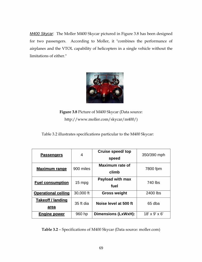
M400 Skycar: The Moller M400 Skycar pictured in Figure 3.8 has been designed
for two passengers. According to Moller, it "combines the performance of
airplanes and the VTOL capability of helicopters in a single vehicle without the
limitations of either."
Figure 3.8 Picture of M400 Skycar (Data source:
http://www.moller.com/skycar/m400/)
Table 3.2 illustrates specifications particular to the M400 Skycar:
PPaasssseennggeerrss 4 Cruise speed/ top
speed 350/390 mph
MMaaxxiimmuumm rraannggee 900 milesMaximum rate of
climb 7800 fpm
FFuueell ccoonnssuummppttiioonn 15 mpg Payload with max
fuel 740 lbs
OOppeerraattiioonnaall cceeiilliinngg 30,000 ft Gross weight 2400 lbs
TTaakkeeooffff // llaannddiinngg
aarreeaa35 ft dia Noise level at 500 ft 65 dba
EEnnggiinnee ppoowweerr 960 hp Dimensions (LxWxH): 18' x 9' x 6'
Table 3.2 – Specifications of M400 Skycar (Data source: moller.com)
69

The benefits of both Skycars are easy to see. Both allow for personal
convenience and time flexibility unavailable by other air transportation systems.
Both are operated on regular automated gasoline, a feature that keeps them cost
efficient and easy to maintain. Skycars are also designed to be relatively quiet.
They possess a multiple ducted fan arrangement that generates little noise "by
using modest thrust loading and tip speeds."
When compared to other modes of transportation, the infrastructure costs
of Skycars is clear. The following chart from Moller.com illustrates one such a
comparison.
Comparison of Skycar & existing modes of transportation
200 miles high speed rail
route : $4 billion
200 miles skycar system : $0.5 billion
Single ferry costs : $80 million
Fleet of 35 skycars : $14 million (handling the same amount of
people)
Jet’s fuel efficiency : 20 pmpg (80% seat occupancy)
Skycar fuel efficiency : 42 pmpg (60% seat occupancy)
Table 3.3 – Comparison of Skycar with other modes of transportation
(Data source: moller.com)
In addition to these benefits, Skycars are also touted as being safe. Moller
International has equipped them with a variety of safety features that cover
virtually every potential problem possible.
70

Moller International has listed the following safety features:
Dual Engines: If an engine fails, the M400 Skycar has seven other engines
available. Each engine is controlled by a computer, and only one is needed for
successful flight and landing.
Redundant Computer Stabilization Systems: The M400 Skycar is equipped with
three computers, and only one is needed to operate the engine. If one computer
should go out, two more are available to operate the Skycar.
Redundant Fuel Monitoring: In Skycars, fuel is constantly monitored for quantity
and quality. If a problem arises regarding fuel, the driver is notified with
sufficient warning.
Aerodynamically Stable: In the unlikely event that insufficient power is available
to hover, the Skycar's aerodynamic ability and good slide slope allows the pilot
to maneuver to a safe area before having to employ the airframe parachutes.
Automated Stabilization: The Skycar's computer system eliminates any
undesirable movement related to wind. The driver need only worry about speed
and direction.
Inherent Simplicity of the Engines: The rotary engines require very little
maintenance with little change of breaking down.
Enclosed Fans: The enclosed fans and engines provide very little risk of injury to
persons standing near the Skycar.
Dual Parachutes: Even in the most desperate of situations, Skycar passengers
can feel confident about their safety. A parachute at the front of the Skycar and a
parachute at the back of it will safely guide the vehicle and its passengers to the
ground in the unlikely event that there is total power failure.
With these considerations, Skycars are advertised as realistic modes of
transportation. However, in a post 9/11 era, it is difficult to imagine how this
mode would be allowed to operate freely in our airspace. Further, the ability of
71

the average automobile driver, most of whom display poor driving skills, to
become an expert pilot is highly questionable.
Solo Trek21:
Figure 3.9 Picture of Solo Trek (Data source: http://www.solotrek.com/)
Millennium Jet Inc.'s Solo Trek XFV (Exo-Skeletor Flying Vehicle),
pictured above in Figure 3.9 is another option to personal air transportation.
Unlike the Skycar, the Solo Trek vehicle transports its single passenger in the
standing position. Like the Skycar, it possesses VTOL capability, and will likely
be used primarily by the military, paramilitary, or emergency services.
The pilot straps himself into Solo Trek, enters his weight and other
security information, and prepares for an easy, efficient, and safe ride. Using
two hand-controls, Solo Trek’s pilot manipulates the machine to take off
vertically, fly to his destination area, and land. This contraption can hover for
up to 2 hours, reach speeds up to 70 knots, and travel up to 120 nautical miles
without refueling.
21 All of the information on Solo trek comes from SoloTrek' website that can be accessed at <http://www.solotrek.com>
72

The engine of SoloTrek uses "heavy fuel," such as kerosene, JP4, Jp5, or
JP8. The engine engages two counter rotating fixed pitch ducted fans that lift the
passenger and transport him to his destination. The machine is quiet, easy to
operate, and easy to maintain.
Table 3.4 details the specifics of SoloTrek XFV:
Length : 60” Width : 104”
Height : 90” Empty weight : 275 lb.
Normal Takeoff weight
: 553 lb. Max gross weight
: 710 lb.
Operator/Pilot : 1 Operator weight : 105-245 lb.
Operator size : 5’ – 6’6” Fuel capacity : 15 gal
Engine power : 120–140 hp Fuel type : JP, Diesel
Max speed : 80 mph Fan operating speed
: 3500-4000
rpm
Cruise speed : 50 –70 mph Max hover altitude
: 8,000 ft
Max Endurance : 2 hrs Max Range : 150 miles
Table 3.4 Specifications of Solo Trek XFV (Data source: solotrek.com)
SoloTrek has been customized to cover a large range of safety concerns.
For one, its control system can be geared for different levels of pilot experience
including novice, intermediate, and advanced. The machine has been built to
carry all male and female pilots within the 5 to 95 percentile range of sizes and
73

weights. Outside of personal concerns, measures are being taken to ensure the
safety of the operator and those around him. A security system is being
developed that would prevent its unauthorized use. The controls of SoloTrek
also prevent the pilot from manipulating the machine to perform any unsafe
maneuvers. If something begins to go wrong with the machine, a system will
alert its pilot to land as quickly as possible. In the event that something with the
machine goes drastically wrong, SoloTrek XFV's "ballistic pilot extraction system
will deploy automatically to provide an additional level of safety for the pilot."
Conclusion
Both SoloTrek XFV and Skycar provide alternatives for personal
air transportation. Their use by security and medical personnel could potentially
improve response time for incident management. Civilians could enjoy them for
their personal convenience and recreation. While civilians use is possible, most of
its uses will likely be in the military and police sectors. SoloTrek XFV offers
exciting possibilities for recreational use, but like the Skycar, its use by the
general populace is questionable.
3.5 Urban Transit Technologies Introduction
Automated People Movers (APMs) is a confusing category of
transportation technology in that several different technologies have been
grouped under its name. Included in this grouping are Personal Rapid Transit
Systems (PRTs), PRTs use the general idea behind APMs; however, PRTs are
envisioned to be more flexible as they can carry smaller groups of people without
requiring a fixed schedule. In this section, we will focus on PRTs and include a
short section on projects that are related to both PRTs and APMs. To understand
74
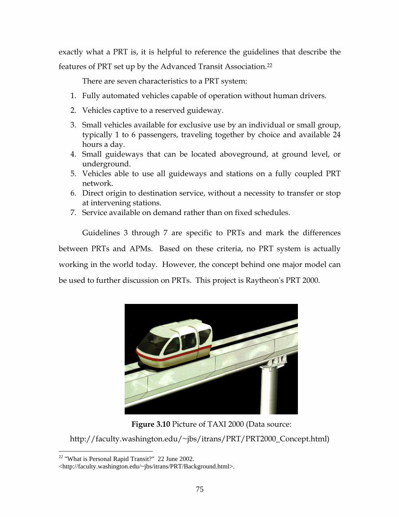
exactly what a PRT is, it is helpful to reference the guidelines that describe the
features of PRT set up by the Advanced Transit Association.22
There are seven characteristics to a PRT system:
1. Fully automated vehicles capable of operation without human drivers.
2. Vehicles captive to a reserved guideway.
3. Small vehicles available for exclusive use by an individual or small group, typically 1 to 6 passengers, traveling together by choice and available 24 hours a day.
4. Small guideways that can be located aboveground, at ground level, or underground.
5. Vehicles able to use all guideways and stations on a fully coupled PRT network.
6. Direct origin to destination service, without a necessity to transfer or stop at intervening stations.
7. Service available on demand rather than on fixed schedules.
Guidelines 3 through 7 are specific to PRTs and mark the differences
between PRTs and APMs. Based on these criteria, no PRT system is actually
working in the world today. However, the concept behind one major model can
be used to further discussion on PRTs. This project is Raytheonʹs PRT 2000.
Figure 3.10 Picture of TAXI 2000 (Data source:
http://faculty.washington.edu/~jbs/itrans/PRT/PRT2000_Concept.html) 22 "What is Personal Rapid Transit?" 22 June 2002. <http://faculty.washington.edu/~jbs/itrans/PRT/Background.html>.
75

In 1993 Raytheon bought the rights to the TAXI 2000 PRT system concept
shown in Figure 3.10. The project was renamed PRT 2000 and was scheduled for
implementation in 2000. However, the project lost funding in 1999 and was
unable to be completed. Nevertheless, the concept behind PRT 2000 can give us
an idea of the possibilities behind PRT systems.
A. Operation of the PRT 200023
The PRT 2000 system consists of lightweight steel guideways and uses
electric motor propulsion and microprocessor control to run small vehicles
capable of carrying groups of up to six people directly to their destinations.
Figure 3.11 illustrates the mechanism of PRT 2000. The system's off-line stations
and integrated network eliminates the need for waiting and line transfers,
hassles that are common to other modes of public transportation. The system's
computerized network delivers passengers to their destinations seamlessly.
Vehicles wait for passengers at off-line stations. Passengers purchase their
tickets for their ride at a machine that is similar to an ATM machine. The
passengers enter their destination information and are given prices accordingly.
After paying for their trip, passengers are given tickets on which their
destinations are encoded. Once passengers enter the vehicle, they insert their
ticket into a slot that reads it. Their journey begins when their vehicle senses an
opening on the main track. Once on the main track, passengers travel non-stop
through an integrated system of guideways until they reach their destination.
After the passengers abandon the vehicles, they either remain at the station of
their last destination or are rerouted by a computer system to stations that are
running low on vehicles.
23 All information on PRT 2000 comes from the University of Washington's web pages entitled "PRT 2000 System Concept" that can be found at <http://www.faculty.washington.edu/jbs/itrans/PRT/PRT2000_Concept.html>.
76

Figure 3.11 Mechanism of PRT 2000, (Data source:
http://faculty.washington.edu/~jbs/itrans/PRT/PRT2000_Concept.html)
B. Benefits of the PRT 2000
One of the benefits to the PRT 2000 is that it is passenger friendly. Because
waiting and line transfers are not necessary, the stress that is typically associated
with other major forms of public transportation is eliminated. The ride itself is
also pleasant. The cars provide room for storing luggage, and seats for each
passenger. Travel is smooth, quiet, and vehicles are available on demand.
Because of the technology employed, the PRT 2000 can run under any weather
conditions. Construction of a system like the PRT 2000 would not interfere with
passengers traveling on roads as the guideways are elevated.
The PRT system also addresses environmental concerns. With
passengers traveling by PRT 2000, the congestion and pollution associated with
highway traffic could be reduced drastically. Because of the use of electric
77

propulsion and steel guideways, the PRT 2000 would not contribute to either
noise or air pollution.
Other Projects
While the PRT 2000 may be seen as an ideal model for PRT systems, other
projects of APMs also provide insight into possibilities for future modes of
transportation. Two types of PRT systems are shown in Figure 3.12. The two
systems that we will briefly describe are Cabintaxi's PRT system and The
Morgantown System.
Figure 3.12 Two types of PRT System
Cabintaxi: The Cabintaxi PRT system that was built in Hagen, Germany in the
1970s illustrates the way a PRT system can make the most of its guideway space.
In this system, vehicles are both suspended below and supported above a
guideway that runs above ground. Cars were designed to travel at 18 mph with
a 2.5 second interval between cars that allowed for emergency braking without
78
collision under all circumstances. While the system was successfully tested,
budgetary cuts in 1979 prohibited its public release.24
The Morgantown System: This system connects the University of West Virginia
with the Morgantown Central Business District. While it is not a PRT system, it
resembles a PRT system more closely than any other working APM system.
Rather than transporting individuals and small groups, the Morgantown System
transports large groups of up to 21 travelers. Built in the 1970s, this system
continues to run successfully today.25
Conclusion
While the Morgantown System is currently the only APM that comes close
to resembling a PRT system, the possibilities for future PRT systems are strong.
While the public often seems unreceptive to other possible modes of public
transportation, research indicates that the PRT 2000 would be quite popular. The
PRT's convenient use makes it irresistible to potential passengers. The
implementation of either PRT systems or other kinds of APMs could alleviate
highway congestion and benefit the traveling public. PRT systems and APMs
have been envisioned for decades and it is likely that the twenty-first century
may finally witness their implementation.
3.6 Freight Pipeline Introduction
Freight pipeline is a generic term used to describe a variety of pipeline
systems through which solids, liquids, and gas can be transported over varying
distances. The concept of tube transportation is not new. For the last two
hundred years pipelines have been used to transport grains, coal, sand, and
minerals. Pipelines of the past have carried these materials for short distances 24 "Cabintaxi PRT System." 22 June 2002. <http://faculty.washington.edu/jbs/itrans/cabin.htm>. 25 "History of PRT." 22 June 2002. <http://www.faculty.washington.edu/~jbs/itrans/PRT/History.html>
79

in pipes with relatively small diameters. Pipelines of the future offer larger
diameters and possess the capability of transporting goods for long distances.
Freight pipeline systems may run on, above, or below ground.
A. Operation
In freight pipeline systems, close fitting capsules or trains of capsules
carry freight through tubes that run underground. These capsules may be
propelled through the pipelines by any one of four different sources of power.
The four different approaches to energizing freight pipeline are 1) hydraulic
capsule pipeline, 2) pneumatic capsule pipeline, 3) electro-magnetic/linear
induction, and 4) maglev technology.
1. Hydraulic Capsule Pipeline (HCP): HCP uses water, oil, or other liquid to
transport closed capsules. HCP is limited in that only capsules with small
diameters can be transported in this manner.
2. Pneumatic Capsule Pipeline (PCP): The freight pipeline system that has
been studied most extensively thus far uses pneumatic blowers as the source of
power. This type of pipeline was employed for approximately fifty years,
starting at the beginning of the twentieth century. During this time period, five
major cities in the United States (Boston, Chicago, New York, Philadelphia, and
St. Louis) employed PCP to transport U.S. mail and parcels between each city's
main post office and its branches. Over time, the pipe systems and their
equipment wore down, and the technology was replaced with trucks, our current
mode for transporting goods.
While PCP has a history of successful use, it requires booster pumps to
transport cargo beyond a distance of several miles. Research has also shown that
PCP systems are also extremely noisy and are not energy efficient. Within a
80
pneumatic pipeline, cargo can travel between 40 and 60 mph. The diameter for a
pneumatic pipeline tube is 2 meters.
3. Linear Induction Propulsion: Linear induction motors are electrical
machines that convert electrical energy directly to in translation motion. The use
of linear induction, or linear synchronic propulsion, has been proposed as an
alternative means of moving capsules within an air filled pipeline. In this
system, an electromagnetic thrust would be induced in each capsule as it passes
over magnetic induction coils set in the pipeline. All capsules pass through the
pipelines at the same speed, and a constant volume of air is maintained between
each capsule. Using linear induction propulsion, a speed of up to around 60
mph can be obtained.
4. Maglev technology: Maglev, a combination of super conducting magnets
and linear motor technology, may be used as a means of transporting goods via
pipelines. Using Maglev technology, capsules could be propelled through
pipelines that are four to six feet in diameter. Capsules could be transported
within a speed range of 120 to 180 mph.
B. Benefits
Freight pipeline systems would drastically improve the transportation of
goods throughout the U.S. Through pipeline systems, freight could be
transported quickly and cheaply, impervious to weather conditions. With a
reduction in the number of trucks carrying freight, the potential for accidents on
highways would also be reduced.
When compared to trucks, freight pipelines are arguably a much better
mode of transportation. In 1996, more than 200,000 highway accidents involved
81

medium and heavy trucks. These accidents resulted in 5,400 deaths.26 The
implementation of freight pipelines as the major means for transporting goods
could eliminate these deaths and improve traffic conditions for all. Freight
pipelines are also environmentally friendly on account of both air and noise
pollution.27
C. Current Projects
A number of projects are currently being conducted in regards to freight
pipeline systems, primarily by the Capsule Pipeline Research Center and the
Federal Highway Administration (FHWA).
Subtrans: The FHWA is currently developing and investigating the possibilities
of a freight transportation system called SUBTRANS. The SUBTRANS system
runs freight-carrying capsules on steel rails in a tube that is about two meters in
diameter. Linear induction motors electrically propel the capsules. The capsules
travel along the main route at a constant speed of 60 mph until they either reach
their destinations or are transferred to another route or terminal. Capsules may
be transferred from one route to the next at the same speed of travel using
electromagnetic switching. The system could carry up to 1875 capsules per hour,
almost equivalent to 16,500 metric tons. After the capsules reach their
destination, they can temporarily be used to store the materials they have
carried.28
Fast Tube System: Richard J. Earle came up with the idea behind this system
that proposes to transport both people and freight in capsule cars through a
26 "The Future of Freight: Research Explores Underground Pipeline System." Texas Transportation Researcher 36.2 (2000). 24 July 2002. <http://www.tti.tamu.edu/researcher/v36n2/underground_freight.stm>. 27 Ibid. 28 Lawrence Vance and Milton K. Mills. "Tube Freight Transportation." Public Roads Online. Autumn 1994. 24 June 2002. <http://www.tfhrc.gov/pubrds/fall94/p94au2.1.htm>
82

pipeline system. Cars with wheels will travel on tracks at a speed of up to 250
mph and deliver passengers to their destination without stopping. Earle
envisions a system of pipelines with tubes for acceleration, deceleration, and line
transfer. Still in the design stage, Fast Tube System is currently looking for
financial backing .
Capsule Pipeline Research Center (CPRC): CPRC was established in 1991 to
study and develop new pipeline technology for underground transportation of
freight. CPRC conducts research in hydraulic capsule pipeline and pneumatic
capsule pipeline. CPRC has two main laboratories, one at Missouri University
Research Park and one at Missouri University's Holstein Farm. The laboratory at
Research Park has an 8-inch diameter, 430 foot length steel pipe for testing
hydraulic capsule pipeline. The laboratory on Holstein Farm has a 3,500 foot
length system.
The laboratory on Holstein Farm is a coal log pipeline pilot plant. At the
plant, coal is compacted into cylinders and transported through a pipeline
system that uses water to move the coal. The high pressure compaction
technology used to compact coal can also be used to compact many other
materials.
D. Research Institutions
In addition to the University of Missouri, several other research
organizations are contributing to the study of freight pipeline systems. These
organizations include Tokyo University, Delft University of Technology, Texas
A&M University, and The International Freight Pipeline Society.
Tokyo University: Tokyo University and the Japanese government have been
developing ideas for underground freight pipeline systems for quite some time.
83

Their most recent proposal is for a smart tube system that would propel capsules
using maglev/linear induction through a semi-vacuum pipeline.
Delft University of Technology: This research institution in the Netherlands has
been conducting research on freight pipelines since the 1980s. Their research
investigates the control technology that is needed to run electric powered cars in
a 5 feet diameter tunnel that connects the main international airport to the freight
terminal.
Texas A&M University: Texas A&M's college of engineering and TTI are
investigating the possibilities of a subterranean freight pipeline system that
would consist of 2 meters of reinforced concrete pipes that are capable of holding
pallet-carrying vehicles.
International Freight Pipeline Society: The International Freight Pipeline Society,
or IFPS, is a research foundation that is conducting technical seminars and
calling for technical papers on freight pipeline.
Conclusion
Freight pipeline systems are currently being investigated by many
institutions. The general consensus is that compared to freight-trucks, they offer
a clean and efficient alternative for freight transportation.
3.7 Automobile Ferry System
Introduction
An automobile ferry system provides a means for travelers to drive their
passenger vehicles on to another mode and let this other mode take them (and
their vehicle) to their destination. Such a system could travel along a link for
84

only a few miles (to span a congested urban corridor) or hundreds of miles to
span intercity distances.
Intercity travel-by-ferry has been conceptualized by a German company
as a number of "pods"moving on magnetic tracks carrying their individual cars, and
self-organizing to form a train as they travel long distances at high speed (upwards of 300
mph). The high speed is made feasible because of magnetic levitation (maglev) and
propulsion technology. Chapter 5 provides more information about both the maglev
technology, and the company, TransRapid.
A company in Houston has proposed an intracity system to ferry cars
across a short but congested link in an urban setting. However, instead of using
maglev technology, they employ (regular) rubber-wheeled trailers powered by
linear induction motors (LIM). The motor itself is situated on the guide-way
railing. Figure 3.13, below displays a picture of the Automobile Transport Unit
(A2). The tractive force of the LIM is transferred to the trailer by an "arm"
connector. Automobiles drive up on to the trailer and, which is then moved by
the LIM to the destination. The system is marketed by A2 Engineering Corp.,
and most of the specifications discussed in the following sections are provided
by them. Some of the unresolved issues with this system are discussed in the
final s
ections of this chapter.
Figure 3.13: Picture showing Automobile Transport Unit (A2)
85

A. Important Features
• Capacity to move 400,000 vehicles per day doubling the freeway capacity.
• Automated operation eliminates the element of driver error.
• Electrically powered reduces mobile source emission.
B. Components
The four components of the A2 system are:
1. Elevated steel guideway which is fast, lightweight and easy to erect.
2. A carrier or trailer which transports the driver and other occupants in
their own car.
3. Linear Induction Motors (LIMs) that pull the carriers along the guideway
using electric power.
4. Local sensors and controllers that signal the motors and carriers to
perform automated functions without relying on central computer control.
The guideway consists of two lanes, a main lane that runs continuously at
70 mph without stopping and an access/exit lane. A steel rail outside each lane
carries LIM. The guide way can be deployed at 16 feet from ground level.
C. Working
There are four major tasks:
1. Driving on to a trailer
2. Automated Coupling
3. Automated Decoupling
4. Driving off the trailer
These tasks can be divided in three categories: Loading, Access and Exit
maneuver. These categories can be explained as follows:
86

Loading
From the service road cars enter the loading area. The driver keys in the
exit destination which can be changed while traveling. The car is remotely
weighed and the fare is displayed for the driver to pay by swiping a card or by
prepayment. The car moves ahead and stops at a safety arm for the loading
position.
A trailer (A2) towed by a LIM emerges halfway from under the loading
dock in a position for the car to roll down onto the deck. When the safety arm
goes up the driver releases the brakes and as the car is on a decline, it rolls
forward onto the deck. When the front wheels of the car touch the A2 stop plate
it moves forward allowing the rear wheels of the car to roll down onto the deck.
The driver pulls a console unit into the window which supplies air conditioning
or heat to the car and also contains a keypad for exit destination, 2-way radio for
communication with a central control room in case of emergency or to provide
information. The A2 signals to the main guideway that it is loaded and ready to
merge into the main traveling lane. The process of loading is estimated to take 10
seconds per car. A schematic showing the loading and unloading process for
the A2 is provided on the next page in Figure 3.14.
87

Figure 3.14: A schematic showing the process of loading and unloading of A2
88

Access
The traveling line has linear induction motors (LIMs) spaced every 30 feet,
moving at a fixed speed along a steel beam, which also serves as a guardrail. The
beam is located on the side of the track and two feet above the guideway surface.
It serves as an electric conductor and guide rail on which the LIMs ride. The
LIMs are fitted with a hydraulically controlled arm (cylinder) that serves as a
hitch to the A2. When A2 reaches at the preset position, a signal is sent to the
traveling lane to get the trailer attached to the empty arm. The attached LIM
accelerates to 70MPH and hands the A2 off to the LIM in the traveling lane. At
any given time the traveling lane may contain loaded A2s, empty A2s or
unattached LIMs.
A car drives onto an A2 causing it to signal an empty LIM in the traveling
lane to prepare for a pick-up. The next empty LIM to pass a controller sends a
signal back to the waiting A2 to accelerate to 72 MPH, which it does. As both
LIMs (the accelerating LIM pulling the loaded A2 and the empty LIM on the
main track) pass a pre-designated point they extend the pick-up arms so that
they almost touch in the center of the two lanes. Both extended arms have
sensory devices that control the speed of the accelerating LIM so that it moves up
against the empty arm. As soon as it touches the extended empty arm a
mechanical spring loaded hitch clasps the arm and simultaneously releases the
hitch from the acceleration LIM. At this point the transfer is completed. Both
LIMs retract the arms into normal positions, which is 90 degrees behind the 5
foot extended arm. The arms are extended by hydraulic pressure on a cylinder
and after 5 seconds the power is turned off the hydraulic pump causing the
cylinder to loose pressure and allow the arm to return to its’ normal trailing
position. This provides for the loaded A2 to be guided into the traveling lane or if
hookup failed, to be returned to the accelerating lane. The purpose is to avoid the
possibility of the A2 remaining halfway into each lane. If the hookup failed, the
A2 would be guided back into the accelerating lane where it would go down to
89

ground level and recycle back to the loading dock. Time lapse from acceleration
to hand off is 12 seconds. Figure 3.15, below presents a diagram explaining the
access of A2.
Figure 3.15: A schematic explaining the access of A2
90

The LIMs in the main lane, traveling at 70MPH, are held in position by
guideway and more importantly by a 5/8 inch cable linking all motors. This
makes it impossible for the motor to malfunction and collide with the A2 in front
or rear. If the tension in the cables is excessive, the motor speed is adjusted to
relieve it. Overall the speed is maintained by the electrical flow to the guideway.
Braking is supposed to be regenerative and the steering passive, simply
following the LIM tow arm. It is not clear how the regenerative power is utilized.
Exiting Maneuver
An A2 nearing the destination sends a signal ahead for an empty LIM in
the exit lane to accelerate to 68MPH. The timing is precise such that the loaded
A2 with the arm extended moves up against the extended arm of the empty LIM.
As soon as the A2 touches the extended arm the hitches are reversed and now
the empty LIM is hooked to the loaded A2. It comes to a stop allowing the car to
roll down.
D. Other Features
All loading ramps will maintain an inventory of empty A2s assuring that
there will always be one ready to load, with no waiting time. All unloading
ramps will likewise have an inventory of empty LIMs to receive exiting A2s. A
Central Control System will monitor the overall system and maintain the
inventory balance at each ramp.
LIMs are ideally suited for this service. Their high torque is used in high
performance roller coasters, aircraft launchers from ships and development work
to launch rockets, including the shuttle, horizontally.
Post tensioned beams are used for guide way construction, and corrosion
is prevented by use of weathering steel.
91

Holding Lot
A holding lot will buffer exiting cars. As soon as the lot reaches 75%
capacity traffic lights will be switched to allow the lot to empty, preventing any
backup on the system.
Off Peak Storage
The A2 system is based on pallet concept. When USDOT surveyed 137
possible transit systems the pallet concept was one of the top four considered.
But the reason it was not chosen was that switching vehicles in and out of
storage in off-peak times would be a massive logistics problem. This issue has
been resolved by parking empty A2s in the access lane.
As demand slows an empty A2 will pull out of the loading ramp and
move onto the access lane. It will move ahead until it approaches an empty A2
stopped in storage position. It will pull up within one foot of the A2 and stop.
Other A2s will follow as the demand slows. Up in front of the empty A2s is an
inventory of LIMs waiting to take loaded A2s from the main lane in the normal
exiting procedure. In the same way the inventory of LIMs will occasionally be
depleted and need to be resupplied. This is done by the first A2 in storage
speeding up to the main lane speed of 72 MPH and handing off the A2 to an
empty LIM on the main lane, exactly as if it was handing off a loaded A2
wanting access to the main lane. The empty LIM in the access lane moves ahead
and join the inventory queue. Figure 3.16, on the following page shows the off
peak storage of A2.
92

Figure 3.16: A schematic showing off peak storage of A2
93

End Of Line Turnaround
All A2s exit the main lane at the last unloading ramp. This is necessary
because the main lane LIMs run at 70 MPH and A2s can not turn at this speed.
The empty LIMS have no problem turning at high speed. When an A2 exits it
stops for the car to unload and if there is no car it proceeds around the track to
the opposite side of the loading ramp. Figure 3.17, below is a diagram
explaining End of Line Turnaround for A2.
Figure 3.17: A schematic explaining End of Line Turnaround for A2
94
Interchange
A2 changes to the main lane by following the access lane until the desired
direction is reached. At this point the A2 is automatically handed off to the main
lane in the selected direction. The exit destinations keyed in takes all this into
account and the A2 is programmed to exit and enter the main lane at an
appropriate time.
Speed Change
Main lanes run at 70MPH. A2s in the access lane can run at 68 to 72 MPH.
A2s in the high speed lane exit and the LIM slows to the lower speed and hands
the A2 off to the slow speed main lane.
E. Safety
As cars can’t leave the road, they can’t hit objects on the sides or roll over.
They can’t be hit head on or from the rear because they are mechanically
separated. They can’t be hit broadside because the guideway is grade separated.
In a power failure situation A2 comes to a controlled stop. The spring loaded
front stop plates will hold the car. The occupants can depart by a ladder leaving
their cars behind. Provisions will be made for emergency departure by lift
devices. If a single A2 loses power the cable linking it with other LIMs will tow it
along. When the power is reapplied it overcomes the spring action, the plates get
flat and the car can drive over them.
F. Benefits
It is convenient and comfortable and requires no transfers. The most
important aspect is having the use of personal car from the beginning to the end
of a trip. The elevated guideway can be erected in an existing right-of-way. 90%
of accidents are caused by driver error, 10% are caused by mechanical error,
these could be significantly reduced on the A2.
95

G. Design and Development
A2 Engineering Corp., Houston, TX, USA.
H. Model Survey
To test the working of A2 a survey was conducted by A2 Engineering
Corp. One of the most congested freeway section in the United States (the I-610
interchange with I-10 and Us-59) was selected as a model for the survey. The
average daily traffic on this section is 572,000 veh/day. No data was provided on
what the ATU would cost to ride the system. The results are as follows:
• 30% of all traffic were trucks
• 20% of the cars were going only to next exit
• 20% were the people who just don’t want to use anything new or different
• 30% or 171,000 vehicle per day will use the A2.
I. System Issues Not Covered Adequately
The maintenance and operational cost of the ATU system is not provided,
nor can it be easily estimated. Unlike Maglev systems, the ATU has many
moving parts which will be subject to wear and tear in the normal course of
operations. The trailers have pneumatic rubber tires which would require regular
maintenance and replacement. The LIMs and the mechanical linking arms
would also be subject to fatigue (similar systems deployed on roller coasters are
periodically taken off-line for maintenance.) The control system required to
activate the linking arm for merging to-and-from the main lane is not explained.
The effects of a support failure (such as failure of the columns due to accidental
or willful collision) could be catastrophic.
96

Conclusion
The ATU system is an innovative concept for ferrying automobiles
through congested urban areas. However, in practice, this may have the
undesired effect of simply moving the congestion from one link (the one spanned
by the ATU) to another (the link where the ATU line ends.) The engineering
components that make up the system are readily available. However, problems
(if any) associated with their integration into a smoothly working system are
difficult to predict, as is the MTBF (mean-time-before-failure) of the system and
its components.
97

Chapter 4
INTRACITY PERSONAL TRANSPORTATION—FUEL CELLS
4.1 Introduction
As noted in the last chapter, the increasing amount of fuel that is being
consumed by the transportation sector. While alternative means of transportation
clearly need to be sought, most Texans do not want to abandon their cars for
conventional methods of public transportation. Fuel cell vehicles provide the
opportunity to continue traveling in their cars while reducing both the consumption
of petroleum and the emission of green house gases.
4.2 Operation
Figure 4.1 Working of a Fuel Cell, (Data source:
<http://www.fuelcells.org/whatis.htm>)
Figure 4.1 illustrates the working of a fuel cell.1 A fuel cell is an electrochemical
device that produces electricity, heat and water by using a combination of hydrogen
and oxygen. On its most basic level, a fuel cell contains an electrolyte membrane, a
1 Fuel Cells 2000. 30 July 2002. Breakthrough Technologies Inc. 1 August 2002 <http://www.fuelcells.org/whatis.htm
98

cathode, and an anode. Hydrogen fuel enters into the anode, and a catalyst coating on
the anode causes the hydrogen atoms to split into protons and electrons. Oxygen from
the air enters the cathode and attracts the protons of hydrogen across the electrolyte.
Meanwhile the hydrogen electrons, prohibited from crossing over the electrolyte, form
an electrical current that is used for energy. The electrons then enter the cathode and a
catalyst causes them to reunite with the hydrogen protons and combine with the
oxygen to make water and heat. Water vapor is the waste that is released.
The hydrogen required for fuel cell systems in vehicles can come from a
variety of sources. Direct hydrogen in the form of liquid or gas simply enters the
system as discussed above. However, hydrogen that is obtained from gasoline, natural
gas, or methanol has to be converted on board the vehicle. This conversion requires a
reformer that adds bulk to the vehicle engine. A variety of institutions are currently
trying to eliminate the need for a reformer in fuel cell systems.
4.3 Advantages of Fuel Cells
Fuel cell vehicles have a number of advantages over internal combustion
vehicles. Because fuel cell engines operate electromechanically, they achieve better
fuel efficiency than internal combustion engines. In the long run, this efficiency will
reduce operating costs. Unlike internal combustion engines, fuel cell engines also
possess the capability of being pollution and odor free. The only byproduct of fuel
cell engines is water, thus the only emissions that is released from fuel cell vehicles
is water vapor. Of course, if hydrogen is obtained from gasoline, a viable option for
fuel cell vehicles, some greenhouse gases are emitted. They is less harmful, however,
than the greenhouse gases that are emitted from vehicles running on internal
combustion engines. Fuel cell engines are dependable, require little maintenance, and
are quieter than internal combustion engines.2
Fuel cells are also a better source of energy than batteries. While batteries
eventually run down, fuel cells keep running as long as fuel is provided. Since fuel
cells are also more resistant to elevated temperatures than batteries, they are more 2 "PEM Fuel Cells." Hpower Corp. 2001-2002. H Power Corporation. 23 July 2002 <http://www.hpower.com/index/shtml
99
dependable in extreme environments. Finally, while battery technology is nearing
the summit of its capabilities, fuel cell technology is in its initial stages of development,
full of possibilities.3
4.4 Types of Fuel Cells
There are several different types of fuel cells, generally categorized by the kind of
electrolyte they use. These include:
• Phosphoric Acid (PAFC)
• Proton Exchange Membrane (PEM)
• Molten Carbonate (MCFC)
• Sodium Borohydride (SBFC)
• Solid Oxide (SOFC)
• Hydrogen
• Alkaline
• Direct Methanol (DMFC)
• Regenerative fuel cells
• Zinc Air fuel Cells (ZAFC)
• Protonic ceramic fuel cells (PCFC)
Of these fuel cells, proton exchange membrane fuel cells and direct methanol fuel
cells will be discussed in further detail because they are more suitable for use in
vehicles.
4.5 Proton Exchange Membrane Fuel Cells
A Proton Exchange Membrane, or PEM, fuel cell is most probably the kind of
fuel cell that will be mass marketed first for vehicles. It has a solid-polymer
electrolyte, which is especially beneficial because it reduces corrosion and prevents
migration risks that are associated with liquid electrolyte fuel cells. It operates at
temperatures between the freezing and boiling points of water, a characteristic that
3 Ibid.
100

enables it to start up very quickly with the help of very little, if any, auxiliary
systems.4
Ford is currently developing what may very well be the first fuel cell vehicle
to be sold on the mass market. The P2000 is projected to run off of tanks for liquid or
gaseous hydrogen. The only emission from the vehicle is water vapor. The car is
scheduled for release in 2004.5
4.6 Direct Methanol Fuel Cells
Another possible fuel cell candidate for car use is a direct methanol
fuel cell. These fuel cells utilize methanol rather than hydrogen. The system does
not require a hydrogen storage tank, nor does it require a reformer. This feature
makes direct methanol fuel cells particularly attractive for vehicle use. However,
problems with direct methanol fuel cells need to be remedied before they can be
mass marketed as car engines.6
The power density, energy conversion efficiency, and fuel utilization of direct
methanol fuel cells need to be increased before they become available for mass
market. In order for these goals to be met, the amount of platinum catalyst needed
to attain a high energy levels needs to be lowered. Also, direct methanol fuel cells
have a problem with methanol passing through the membrane of the fuel cell
without producing electricity.7 However, some companies working with direct
methanol fuel cells claim that they have solved this problem.
4 Ibid. 5 "Fuel Cell Cars." Howstuffworks. 1998-2002. Howstuffworks, Inc. 25 July 2002 <http://www.howstuffworks.com/news-item10.htm 6 "Technical Advances Improve the Potential for a Fuel Cell which Eliminates the Need to Store or Generate Hydrogen." Office of Transportation Technologies. April 2001. 1 August 2002 <http://www.ott.doe.gov/success.html 7 Ibid.
101

Daimler Chrysler used a direct methanol fuel cell car when it achieved the
status of being the first company to produce a fuel cell vehicle to drive across the US.
They, and several other automotive companies are currently competing to be the
first to release direct methanol fuel cell vehicles onto the mass market.8
4.7 Cost of Fuel Cell Technology
To estimate the costs of fuel cell technology, a study written by J. Fernando
Contadini that was published by the Methanol Institute at Methanol.org was
consulted.9 In this section, brief summaries of this material are provided along with
the charts and the alphabetized notes accompanying them that are published.
The Methanol Institute's study looks at the integration of both methanol and
hydrogen powered fuel cell vehicles into the automobile industry for approximately the
next fifty years. The study considers that the market for automobiles will include
Hybrid Electric gasoline vehicles, conventional internal combustion vehicles, and
gasoline fuel cell vehicles in addition to methanol and hydrogen powered fuel cell
vehicles. The study also distinguishes between direct and indirect methanol fuel cell
vehicles. Indirect methanol systems utilize a reformer; direct methanol systems, as
discussed in the section on direct methanol fuel cells, do not need a reformer.
The first area of concern is the market penetration of alternate fuel vehicles.
The Methanol Institute has published three charts in consideration of the market
penetration of new vehicle technology. This first chart, shown in Figure 4.2, illustrates
the future possibilities for vehicles using advanced gasoline.
8 Methanol Institute. 23 July 2002 <http://www.methanol.org/f-index.html 9 Contadini, J. Fernando. "Social Cost Comparison Among Fuel Cell Vehicle Alternatives." MI: Fuel Cells. 1996-2002. Methanol Institute. 28 July 2002 <http://www.methanol.org/fuelcell/special/contadini_pg1.html
102

Figure 4.2 Market Penetration of Advanced Gasoline, (Data source: www.methanol.org)
As Figure 4.2 illustrates, fuel cell vehicles using advanced gasoline reach 100%
market share in 2027, skyrocketing from 0% only seven years earlier. ICV Hybrids
reach 60% in 2010 and stay there until 2021 when they begin to drop, reaching 0% in
2027. Imprv-ICV increase in market share from 25% in 2003 to 65% in 2006, drop to
40% in 2012, and fall to 0% in 2024. ICV-conv begin dropping from 70% market
share in 2003 to 0% market share by 2012.
Figure 4.3 considers the market share with hydrogen used as the fuel for fuel cell
vehicles.
Figure 4.3 Market Penetration of Hydrogen, (Data source: www.methanol.org)
103

Figure 4.3 illustrates that the integration of hydrogen as the fuel for fuel cell
vehicles tremendously alters the market share for fuel cell vehicles using gasoline.
In this scenario, fuel cell vehicles using gasoline only reach a market share of 40% in
2027 and fall fairly rapidly to 0% in 2033. Statistics for other engine types are slightly
altered, witnessing a more gradual decline in market share.
This third chart, Figure 4.4, considers the integration of fuel cell vehicles
powered by indirect methanol and direct methanol. Hydrogen has been excluded from
this analysis, excluding the possibility that both hydrogen and methanol could share the
market. This exclusion is necessary in order to truly compare the hydrogen and
methanol markets.
Figure 4.4 Market Penetration of Methanol, (Data source: www.methanol.org)
Figure 4.4 indicates indirect methanol fuel cell vehicles reach 20% by about 2016
and fall to 0% by 2027. Direct methanol fuel cell vehicles follow almost the exact
pattern of hydrogen fuel cell vehicles. The exception to this is that direct methanol fuel
cell vehicles do not begin to rise in market share until 2015 compared to hydrogenʹs
beginnings in 2003.
The second area of the Methanol report with which we are concerned is that
of the cost of new vehicles. This report from Methanol considers three studies done
on fuel cell vehicles that projected estimates on their individual costs. Table 4.1 is a
104

comparison of three reports and a given "assumed." The alphabetized notes come
directly from the Methanol report.
Vehicle Gasoline Methanol Hydrogen
($/car) ICV
convent.
ICV
Tech-
1
Hybrid
ICV
FCV Indirect
FCV
Direct
FCV bFCV
DTI
(1998)
18,000 - - 22,400
to
24,500
20,800
to
21,600
- 20,000
Ogden
(1998)
18,996 a 19,196 b
- 19,474
to
19,814
19,124
to
19,224
- 19,996
Lipman
(1999)
20,558 c - - - - 24,495 d
24,570 d
Assumed 18,996 19,196 20,194 e
21,800 20,500 20,000 20,000
Table 4.1 Comparison of cost of new vehicles, (Data source: www.methanol.org)
Assumptions
a. The study gives the incremental cost over the gasoline without specifying it. The assumed cost of $18,624.00 (1997$) is based on the average price for a new vehicle according to American Automobile Manufacturers Association (AAMA), (1997).
b. The cost is an increment of $200.00 over the cost of the conventional ICV. The value was established based on the comments found in Ogden (1994).
c. The Ford Taurus was chosen to represent this category. d. The cost is calculated for a maximum 300,000 vehicles. To represent much
higher production levels, the chosen study values are from the low case and high production volume scenario.
e. The cost assumed is based on the relation between the incremental cost of a Fuel Cell Hybrid Vehicle and the ICEHV found in Henry K. Ng et al (1996).
105

Table 4.1 illustrates, the individual costs for each vehicle come within a range of
$2,000 of each other.
The cost of vehicle maintenance is the next area of concern. While the
Methanol Institute does not provide data on vehicle maintenance, it does offer an
estimation of yearly vehicle maintenance costs based on different studies. These
estimates may be organized into the following list:
• Conventional ICEV--$516.00 • Hydrogen FCV--$434.00 • Indirect Methanol FCV--$450.00 • Hybrid Electric ICE Gasoline Vehicle--$452.00 • Gasoline Fuel Cell Vehicle--$530.00 • Direct Methanol FCV--$434.00
Maintenance costs for all vehicle types fall within $100.00 of each other. The
costs estimated for direct methanol fuel cell vehicles and hydrogen fuel cell vehicles
are the lowest, with Indirect Methanol fuel cell vehicles and hybrid electric ICE
gasoline vehicles falling close behind. The maintenance costs for Conventional
ICEVs and gasoline FCVs are estimated as the highest.
While vehicle maintenance will necessarily be important to consumers, so
will the cost of fuel. Table 4.2 from The Methanol Institute, compares estimates of fuel
prices based on several studies. The estimates for fuel costs have taken into
consideration price variables such as projected feedstock costs, conversion costs,
transportation storage and distribution costs, and taxes. Again, the notes associated
with Table 4.2 come directly from the Methanol Institute.
106

FUELS Hydrogen Methanol Gasoline
($/gal-eq) Centr.
Plant
Decentr.
Plants
Currently Future a
DTI - 0.98 0.94 1.27 0.80 to
1.20
Ogden 1.60 to
5.20
1.70 - 1.25 1.05
Lipman b - 1.05/1.32 1.37/1.90 1.37/1.90 -
Sigworth 3.30 - - 2.08 1.46
Kalhammer > 3.00 - - - -
Assumed c 3.00 to 1.70 1.00 1.50 to
1.20
1.20 to
1.40
Table 4.2 Comparison of fuel prices, (Data source: www.methanol.org)
Assumptions
a. After worldwide methanol demand increases over 5 x 10⁶ metric tons/year. b. High volume production. c. The initial cost of reformulated gasoline at $1.20 per gallon, and the incremental
cost of 1% a year until a constant cost of $1.40 per gallon in the future. Oil prices will remain constant due to increase in supply with the introduction of alternative fuels. For methanol from natural gas (NG), it assumes the cost of $1.00 per gal-geq until a fleet of 1.5 million methanol vehicles is achieved by 2007, and $1.50 per gal-geq for the following 10 years due to the necessity to build new plants. By 2017, a decremental cost of 2 % per year is applied until the cost reaches $1.20 per gal-geq. For hydrogen from NG, the initial cost of $3.00 per gal-geq was assumed, with the decremental cost of 2 % per year until it reaches $1.70 per gal-geq. Also, it is assumed that solar hydrogen will be introduced by 2020, at a cost of 2.20 per gal-geq, and will improve 2 % per year until $1.70 per gal-geq. No discount rate was applied. (all from Methanol Institute)
In addition to providing all of these cost estimates, the Methanol Institute
published Table 4.3 that illustrates a straight comparison of all of the different factors in
cost for reformulated gasoline, hydrogen, and methanol powered vehicles. This
comparison illustrates the estimates for cost over about the next fifty years. The
category "Private/Cost" is the combined total of new vehicle cost, maintenance cost,
and fuel cost. The category "Health Dam." considers the health damages associated 107

with the air pollution that is a result of the emissions of each vehicle type. The "Social"
category, the total of private costs and health damages, gives a final estimation on total
vehicle costs.
1998 US$
Billions
New
Vehicles
Maintenance Fuel Private/Cost
Health
Damage
Social
Cost Cost Cost (Monetary) Cost Cost
Reformulated.
Gasoline
19,846.68 7,994.76 4,445.87 32,287.31 720.50 33,007.81
Hydrogen 17,893.07 7,305.05 4,182.33 29,380.45 637.23 30,017.67
Methanol 18,240.73 7,306.99 4,017.96 29,565.68 633.58 30,199.27
Table 4.3: Comparison of cost for reformulated gasoline, hydrogen, and methanol
powered vehicles, (Data source: www.methanol.org)
As Table 4.3 illustrates, a change from reformulated gasoline to hydrogen or
methanol will save a tremendous amount of money in the future. Almost $3 trillion can
be saved on costs such as maintenance, fuel, and vehicle price. Costs related to health
damage are approximately $85 billion less for a community that drives on hydrogen or
methanol powered vehicles.
While health costs associated with gasoline powered vehicles are
tremendously higher than hydrogen and methanol fueled vehicles, the difference in
health costs between hydrogen and methanol fueled vehicles is relatively small.
Methanol powered vehicles are slightly more cost effective than hydrogen when it
comes to health damages.
However, hydrogen saves more money than methanol in the private cost
category. This result is mainly due to the costs of the actual vehicles. Figure 4.5 from
the Methanol Institute illustrates how much money is saved over a 50 year span in the
private cost category by hydrogen and methanol powered cars.
108

Figure 4.5 Savings ov
While Figure 4.5 m
slightly more than methano
According to the Me
the comparison of hydrogen
include the catalyst and sto
estimation on price differe
Institute’s information on th
the Office of Advanced Aut
a price breakdown of the i
fuel cell component costs
production increases. The i
uses reformulated gasoline
10 "Researchers Seek Realistic ManuEstimates. April 2002. Office of Ad<http://www.cartech.doe.gov/researc
Savings over Gasoline Scenario
er gasoline scenario, (Data source: www.methanol.org)
akes it seem as if hydrogen fuel cell vehicles will save
l fuel cell vehicles, the differences are very slight.
thanol Institute, other factors that need to be considered in
powered fuel vehicles and methanol powered fuel vehicles
rage needed for each. As the technology is new, an exact
nces is unlikely at this time. In addition to the Methanol
e market penetration and overall costs of fuel cell vehicles,
omotive Technologies, OAAT, was consulted in order to get
ndividual parts for fuel cell vehicles.10 Table 4.4 addresses
and demonstrates the way the costs will decrease as
nformation presented pertains to a PEM fuel cell system that
as fuel.
facturing Estimate for Automotive Fuel Cell System." OAAT-Fuel Cell Cost vanced Automotive Technologies. 23 July 2002 h/fuelcells/mfg-costs.html>
109

Reformer/Fuel Cell Cost Estimates
Annual Production Rate
500 10,000 30,000 500,000
Fuel Cell Stack $17,258 $9,618 $9,394 $8,509
Air Loop $1,160 $821 $734 $529
Water Loop $1,106 $832 $757 $605
Coolant Loop $620 $486 $450 $386
ATR $3,531 $1,945 $1,532 $1,322
Reformate Loop $1,172 $838 $739 $658
Fuel Loop $879 $616 $573 $466
Controls $719 $501 $442 $316
Misc./BOP $320 $240 $220 $150
System Assembly $723 $487 $442 $157
Total Cost $27,489 $16,384 $15,282 $13,099
Cost/kW $550 $328 $306 $262
Based on a 50kW-net system. All costs are preliminary, as DFMA optimization had not yet been completed. ATR and fuel cell stack examined in more detail than other system components. All costs include 10% cost contingency and markup to reflect profit, G&A.
Table 4.4 Reformer/Fuel cell Cost Estimate, (Data source:
<http://www.cartech.doe.gov/research/fuelcells/mfg-costs.html>)
Table 4.4 shows that total costs reach $27,489 with an annual production rate of
500. As the production rate increases to 500,000, the total cost decreases to $13,099.
Direct Technologies Inc., working with OAAT, is currently exploring ways to decrease
costs and is also looking at the costs for systems that use direct hydrogen.
110

4.8 Conclusion
Whether powered by gasoline, methanol, or liquid hydrogen, fuel cell
vehicles may play an important part in our intracity transportation in the near future.
Methanol and hydrogen powered vehicles are clearly the preferred choice for fuel
cell vehicles. Either source of fuel will reduce the costs associated with health
damages that can be attributed to air pollution.
111

Chapter 5
MAGNETIC LEVITATION (MAGLEV)
Figure 5.1 An illustration of proposed Maglev in Shanghai,
(Data source: Shanghai Maglev)
5.1 Introduction
Concerns voiced in chapter 2 about the damage to the environment and the
depletion of energy sources due to an increase in driving may be answered by
Maglev technology. Maglev systems can transport people and freight between
major cities without hurting the environment or consuming petroleum.
Maglev vehicles may reach speeds of 300 miles per hour and possess safety features
that answer concerns about other high speed rail options available today. Figure 5.1
provides an illustration of the proposed Maglev system in Shanghai.
112

5.2 Technology1
Figure 5.2 The three basic principles involved in Maglev,
(Data source: The Science of Maglev)
The technology behind Maglev operation is relatively simple. Maglev
vehicles operate with superconducting magnets, simple coils of superconducting
wire, and compact cryogenic coolers. Electric power from a substation is supplied to
the vehicle through the guideway. Batteries within the vehicle recharge the magnets
while they are in motion. The hardware required for Maglev operation is
dependable and commercially available. Figure 5.2 illustrates the three basic principles
involved in Maglev.
Maglev systems can be classified according to their physical structure and their
levitation and propulsion systems. Figure 5.3 illustrates the two basic types of
levitation systems: EMS (electromagnetic systems) and EDS (electrodynamic
systems).
1The information in this technology section has been summarized from a variety of sources, including: Freeman, Richard. "The Science of Maglev." The American Almanac. 1993. American Almanac Readings. 20 August 2002 <http://www.members.tripod.com The Pennsylvania Project—High Speed Maglev. 2002. Maglev, Inc. 20 August 2002 <http://www.maglevpa.com/propul.html Maglev2000 of Florida Corporation. 2001. 20 August 2002 <http://www.maglev2000.com/works/how.html
113

EMS systems run on a T-shaped ferromagnetic guideway and depend on
attractive force. Electromagnets line both sides of the vehicle, and ferromagnetic
stator packs are fixed along the underside of the guideway. When the
electromagnets are activated an electrical current passes through the guideway, the
electromagnets are attracted upward to the guideway, and the vehicle levitates.
Figure 5.3 The two basic types of levitations in Maglev,
(Data source: The Science of Maglev)
In contrast to the EMS systems, EDS systems use a U‐shaped guideway and
depend on repulsive force. The sidewalls of the guideway are lined with 8ʺ levitation
coils, and the vehicle contains superconducting magnets. The magnets run along the
center of the coils until an electric current is induced as the vehicle moves forward. The
electric current causes the coils to temporarily act as electromagnets that push the
vehicle upward. At the same time, the superconducting magnets pull them upward,
and the vehicle is levitated. Levitation systems require electronic monitoring that
ensures that a constant gap of about 10 mm is maintained between the vehicle and the
guideway.
The Maglev is propelled in a similar manner. Two kinds of motors can be
employed to propel a Maglev vehicle: a linear synchronous motor (lsm) or a linear
induction motor (lim). LSM uses long stator propulsion, while the LIM uses short
stator propulsion.
114

A system with an LSM uses an electrically powered linear motor winding in the
guideway. A system with a LIM uses a linear induction motor onboard the
vehicle. The LSM as shown in Figure 5.4 is preferred for high speed maglev
systems. However, the construction costs for the guideway are more expensive for this
kind of system. In contrast, systems with a LIM have higher operating costs as the LIM
is heavy and decreases the vehicle's payload capacity.
Figure 5.4 The linear motor winding guideway used by LSM,
(Data source: The Science of Maglev)
In both systems, power is ignited when a three phase alternating current,
controlled from a substation, is sent through the motors. The levitation magnets
within the systems are activated by this current, and the vehicles are propelled along
the guideway.
115
The speed of the vehicle is determined by the intensity of the electrical
current that is controlled from the substation. When the traveling field is slowed
down, the motor becomes a generator. The vehicle brakes smoothly and safely. If
the system or power fails, the vehicles are equipped with independent backup brakes.
As a Maglev vehicle is propelled down its guideway, the magnets that
levitate the vehicle also guide the vehicle by attraction or repulsion, depending on the
vehicle's system type. If the vehicle ever begins to move off center, sensors on the
guideway are activated to draw the vehicle back into its place.
5.3 Areas of Technological Development2
The following list emphasizes the areas in which the future of maglev technical
development will be focused:
• Magnets: High temperature superconductivity, cryogenics, low temperature refrigerators, and superconducting magnet design and construction.
• Materials: Fiber reinforced plastics for vehicles and structural concrete. • Electronics: Communication and high power solid-state controls. • Engineering: Vehicle design (aerodynamics and noise mitigation), precision
manufacturing, construction and fabrication of concrete structures.
5.4 Magnets3
Work is currently being done in the United States and other countries in
magnet technology. Superconducting magnets can be improved upon in order to
improve their efficiency for Maglev technology. The development of vibration
insensitive magnets would be beneficial for Maglev technology. Also, concerns
about the cryogenic refrigeration needed on-board the Maglev vehicles are being
addressed. Designs for systems using supercritical, rather than liquid, helium have
been proposed. This change would increase the efficiency of the cryogenic system.
Efforts are also underway to develop a high-temperature superconductor capable of
2 The list in this section has been taken from the following website: "The Potential for Maglev Applications." Inventors. 2002. About, Inc. 20 August 2002 <http://ww.inventors.about.com/library/inventors/blrailroads.htm 3 The information on Magnets has been summarized from the above website.
116

operating at a temperature above 77 degrees Kelvin. One of the system designs that
have been proposed might be capable of using conductors as they currently exist.
5.5 The Guideway4
The comfort of a ride on the Maglev vehicle depends on the guideway
structure. The guideways are made of high precision steel beams that are mounted
on bearings on concrete columns and foundations. A fixed bearing is fixed
underneath the center of the beam, and a loose bearing is placed at each end of the
beam. The loose bearings at the ends allow for thermal expansion. Accompanying
equipment for levitation, propulsion, guidance, and battery charging are welded
within the guideway beams. Typically, the beams are 203 feet long or 82 feet long.
Figure 5.5 The three main types of guideways,
(Data source: The Pennsylvania Project-High Speed Maglev)
Guideways usually run 7 to 66 feet above ground. For a guideway to be
constructed at a level higher than 66 feet, additional support structures such as bridges
would have to be employed. Figure 5.5 illustrates the three main types of guideways.
4 Information for this section has been taken from The Pennsylvania Project—High Speed Maglev.
117

5.6 Vehicle Structure5
The vehicles are made of aluminum or fiber reinforced plastic structures and
contain all of the necessary equipment including superconducting magnets,
cryogenic systems, and central communications and control systems. While the
vehicles vary in style depending on purpose (freight or passenger transport), the
basics are constant vehicle to vehicle.
End section Middle section
Length 26.99 m 24.77 m
Width 3.70 m 3.70 m
Height 4.16 m 4.16 m
Empty weight 48.0 t 47.0 t
Payload capacity 14.0 t 17.5 t
Passenger Capacity
(seated and standing)136 150
Total weight 62.0 t 64.5 t
Table 5.1 The specifics of the middle and end sections for Maglev vehicles,
(Data source: The Pennsylvania Project-High Speed Maglev)
Maglev trains are made up of separate sections, with a total possibility of 10
sections. Table 5.1 gives the specifics of the middle and end sections for Maglev
vehicles. The sections at the ends of the trains each contain a compartment for a
driver, an operation control system, and a payload area for passengers or freight.
Drivers do not drive the trains but watch the operator console to make sure the
vehicle is traveling according to plan. The middle sections are constructed in the 5 Ibid
118

same way as end sections; however, they vary vehicle to vehicle depending on the
purpose.
Passenger Vehicles6
The design of Maglev passenger vehicles provide a comfortable atmosphere for
travelers. The inside of the vehicles are bright and open, and travelers have
plenty of room to move around during their trip. The seating in passenger vehicles
is flexible, allowing the operator of the vehicle to tailor the arrangements to fit
individual needs. Seats can be broken up into first, business, and economy class
sections. There is room for 64 seats in first class and up to 126 for the economy class.
Seating arrangements can be constructed with or without tables and can be adjusted
to suit the needs of the customers. Maglev passenger vehicles also feature passenger
information and entertainment systems. Personal traveling necessities such as
telephones, restrooms, and on-board catering can easily be incorporated into the
structure of the vehicles.
Transrapid intercity trains can serve as examples of passenger vehicles.
These trains have room for overhead luggage, storage areas for larger luggage, on-
board toilet facilities, first class seating with 2 + 2 seating per row, and economy
class seating with 2 + 3 seating per row. The restroom facilities allow easy access for
passengers with limited mobility. They have closed-circuit fresh and waste water
systems, minimum water use flush systems, and are easy to clean and maintain.
Cargo Trains7
Cargo/freight trains can either carry all freight or can carry part freight and
part passengers. The vehicles are equipped to transport standard aircraft shipping
containers or pallets. They can carry a maximum of 17.5 metric tons of high priority
6 Ibid. 7 Ibid.
119

or express goods. Cargo trains, like passenger trains, can travel at speeds up to 300
miles per hour.
5.7 The Future of Maglev8
Proponents of Maglev envision a National Maglev Network that would
transport people and goods between major population areas. The implementation
of such a system would benefit the U.S. both environmentally and economically.
Because a National Maglev Network could transport freight more quickly than the
current trucking system, the U.S. could save time and money in transport costs.
Productivity would also increase.
While the implementation of a National Maglev Network is currently only a
vision, current research and development in the U.S. and other countries suggest
that such a network may come into reality in the future.
5.8 History9
Before looking at current projects, it is helpful to consider the history of
Maglev development throughout the U.S. and other countries. In the early 1900s
U.S. citizen Emile Bachelet came up with the first idea for magnetic levitation
transportation. He envisioned an EDS system; however, the power needed to
realize his plan was not available at the time. It would not be until the 1960s that
Bachelet's ideas for an EDS system would be realized.
In the meantime, an EMS system was planned in Germany. In 1922,
Herman Kemper conceived of the first attractive mode Maglev. Kemper worked on
his project for the next thirty years, producing a design for practical EMS Maglev in
1953. In 1969, the Transrapid was built.
The sixties proved to be productive for U.S. research in Maglev
technology as well.
8 Information in this section has been summarized from Maglev2000 of Florida Corporation. 9 Information in this section has been summarized from The Monorail Society—Technical Pages. 20 August 2002 >http://www.monorails.org/tMspages/TPMagIntro.html
120

In 1963, James Powell and Gordon Danby of Brookhaven National Laboratory
brought Bachelet's vision for an EDS system into reality. Powell and Danby
discovered that superconducting magnets would provide the power necessary for
Bachelet's ideas. In 1966, they presented their design for an EDS system with
discrete coils that ran on the guideway. Powell and Danby continued with their
work and were awarded a patent in 1968. The Japanese eventually implemented
Powell and Danby's concepts for their own Maglev system.
In 1965, the High Speed Ground Transportation (HSGT) Act was enacted in the
U.S. to provide funding for HSGT projects and research, including rail, air cushion
vehicles, and Maglev. Under this act, several Maglev projects, listed below, flourished
throughout the late sixties and early seventies. A continuous sheet guideway (CGS)
system in which the moving magnetic fields of vehicle magnets induce currents in a
continuous sheet of conducting material was conceptualized by groups from Stanford
University, Atomics International, and Sandia National Laboratories in 1969. One-
twenty-fifth scale models of this system were constructed and tested at speeds up to 27
miles per second by a variety of groups, including one from MIT.10 At the same time,
Rohr, Boeing, and Carnegie-Mellon University were developing an EDS system. In the
early 70s, the Federal Railway Administration (FRA) provided the Ford Motor
Company and the Stanford Research Institute with funding to develop EDS and EMS
systems. Eventually the linear electrical motor, used by all maglev prototypes today,
was developed as a result of FRA funding. However, in 1975, the federal government
discontinued the HSGT Act, bringing government sponsored Maglev research to an
end.
While very little research was done in the U.S. in the late 1970s and 1980s
on Maglev technology, countries such as Great Britain, Canada, Germany, and Japan
continued in their research and development. Of these countries, Germany and
10 The CSG concept is a part of the Magplane design.
121

Japan have garnered the most attention. The following timeline11 details Japan's
development of Maglev technology:
1972- Experimental superconducting maglev test vehicle ML-100 succeeded in 10 cm levitation.
1977- Test run of ML-500 vehicle on inverted-T guideway
1979- Unmanned ML-500 test vehicle achieved speed record of 517 km/h (321 mph)
1980- Test run of MLU001 vehicle of U-shaped guideway
1987- Speed of 400.8 km/h (249 mph) achieved by 2-car manned vehicle
1990- Yamanashi Maglev Test Line (YMTL) construction plan approved
1996- 18.4km section of YMTL completed; MLX01 (3 cars) delivered
1997- Tests of MLX01 started. Speed record of 550 km/h (342 mph) on 12/24/97
1999- New speed record of 552 km/h (343 mph) in Transrapid Maglev Test Line
Currently, Japan is using an EDS system design. In contrast, Germany uses
an EMS maglev design. The following list12 details the development of Maglev
technology in Germany:
1969- Transrapid 01- Built by Krauss-Maffei, first practical EMS levitation vehicle
1971- Transrapid 02- Operated by K-M on a 0.93 km track with EMS, max speed
164km/h
1972- Transrapid 03- Operated by K-M on .93 km track, max speed 140km/h
1973- Transrapid 04- Operated by K-M on a 2.4 km track, EMS support
1975- HMB1- First vehicle with long armature LSM and EMS by T-H
1976- HMB2- First passenger-carrying vehicle by Thyssen-Henshel
1979- Transrapid 05- Emsland Test Facility started; Carried passengers up to 75km/h
1983/4- Transrapid 06- First 21.5 km of Emsland opened; 302km/h achieved
11 This exact timeline may be found on the aformentioned website. 12 Ibid
122

1993- Transrapid 07- Achieves speed of 450 km/h
1999- Transrapid 08- Current system; Is the only COTS system available today.
Germany's Transrapid 07 system is planned for implementation in Orlando,
Florida. The early 1990s witnessed an increase in interest in Maglev in the U.S. The
following section details some of the recent and current Maglev projects in the U.S.
5.9 U.S. Projects13
In 1990, the U.S. Department of Transportation began generating interest in
Maglev technology when it submitted a report that considered the possibilities of
constructing a high speed intercity Maglev transportation system in the U.S. After
submitting the report, the U.S. Department of Transportation joined with several other
agencies, including the U.S. Army Corps of Engineers and the U.S. Department of
Energy, to form the National Maglev Institute (NMI).
As congestion and environmental problems continued to increase in the U.S.,
the possibilities for Maglev systems began to become clearer. In December of 1991,
the Intermodal Surface Transportation Efficiency Act (ISTEA) allotted $725 million
for a program to develop Maglev prototypes. Funding for Maglev research and
development continued to grow.
Initially, doubts about Maglev were voiced. Once these doubts were
answered, more funding became available for Maglev development and research. In
1998, Congress passed the Transportation Equity Act of the 21st Century. This act
allotted $218 billion for states and localities to use for surface transportation
assistance over the next six years. Section 1218 of this act created a National
Magnetic Levitation Transportation Technology Development Program. This
program sought out applications for a grant to fund Maglev development. Out of the
applications received, seven finalists were chosen. Funding for preconstruction
13 The following information has been summarized from Transrapid-USA. 20 August 2002 <http://www.transrapid-USA.com/flash_index.html
123
planning was provided to the seven finalists from Maryland, Pennsylvania, California,
Florida, Georgia, Louisiana and Nevada. Once a year of planning had passed, each of
the finalists submitted their proposals to the Federal Railroad Administration (FRA) in
June 2000. From these finalists, the FRA chose Pennsylvania and Maryland for the
implementation of Maglev technology. The remaining five were allotted almost $1
million each to further their projects.
The Maryland and Pennsylvania projects are currently in the Environmental
Impact Statement (EIS) stage of development. The Secretary of Transportation may
choose one of the projects for further design and construction. The technology for
both projects is being provided by Transrapid International.14 The systems being
proposed will use synchronous long strator linear motors. The projects are discussed
in further detail in the following two sections.
5.10 The Maryland Project15
Background
The Maryland Department of Transportation, District of Columbia, Baltimore
City, Baltimore County, and the Maryland Transit Administration have joined
together to work on this project. The 40 mile long system that is proposed will link
Camden Yard in Baltimore and Baltimore-Washington International (BWI) Airport, to
Union Station in Washington D.C. Stations will also be set up at the airport and near
the Capital Beltway. Figure 5.6 illustrates the areas covered by this envisioned system. The
system will work as a part of a larger transportation system that includes urban,
commuter and intercity bus and rail systems in Baltimore, Washington D.C., and the
BWI Airport.
14 In 1998 system houses Adtranz, Siemens, and Thyssen joined together to form Transrapid International. 15 Information in this section has been summarized from The Baltimore-Washington Maglev Project. 2001. BW Maglev. 20 August 2002 <http://www.bwmaglev.com
124

Figure 5.6 Proposed eastern seaboard Maglev corridor,
(Data source: The Baltimore-Washington Maglev Project)
If this system is implemented, the organizations involved hope to eventually
integrate it into a larger Maglev system that would serve the entire Northeast
Corridor between Boston, MA and Charlotte, NC. Some of the major cities served
would be: New York City, Philadelphia, Wilmington, Baltimore, Richmond and
Charlotte. The system, entitled the Eastern Seaboard Maglev Corridor, would be a
total of 800 miles long and would provide both passenger and freight transportation.
125

Alignment for the Maryland project was finalized at the end of May 2002.
Initially, the I-95 parallel alignment and the Baltimore-Washington Parkway parallel
alignments were considered for the project. However, these alignments have been
discarded. Currently, the Amtrak parallel alignment is being studied. The Amtrak
Parallel alignment, which runs through Prince George's County and Anne Arundel
County, is about 37.5 miles long with stations located at Baltimore-Washington
International Airport, downtown Baltimore, and the Union Station in Washington, D.C.
Project Costs
The cost estimates for the Maryland project include the following:
• Technology Systems, including vehicles, control system, propulsion system, communication system and energy system
• Guideway Structure, including superstructure, substructure and foundation • Passenger stations, maintenance facilities & substations • Operation & Maintenance costs • Replacement for various systems
Certain assumptions have also been made with regard to the cost estimates.
These assumptions are as follows:
• I-95-parallel alignment (this has now been discarded and the Amtrak parallel alignment has been retained for further study)
• 40 Mile long steel guideway • Stations at the three aforementioned locations. • 18 hour operation • Three section train sets
126

When projected to 2006, the total capital cost, based on a 40% contingency for
all civil/structural costs as well as operation and mechanics costs, is estimated at
$3.5-4 billion, or $88 million per mile. Figure 5.7 breaks down the variables for expected
cost.
Figure 5.7 Variables for expected cost (broken down) for Maryland Project,
(Data source: The Baltimore-Washington Maglev Project)
127

Project Benefits
The organizations involved with this project see both short and long term
benefits from its application. The construction of this system could help the Baltimore-
Washington area in their bid for the 2012 Olympics. With a Maglev system in place,
Olympic spectators and athletes could travel easily between the airport and event
locations. Maglev would also help the Baltimore-Washington area in general in terms
of business, recreation, tourism, and commuter travel, all of which are projected to
increase over the next forty years.
Additional benefits include:
• Meeting transportation demands from growing population, employment, tourism and air travel.
• Reducing congestion on area roadways. • Helping to reduce the need for additional airport and highway construction. • Supporting BWI Airport as a key economic engine of the State. • Distributing airline passengers evenly among the region's three airports. • Supporting Smart Growth principles by focusing transportation access to the
revitalized areas in Baltimore, and Washington, D.C. • Promoting tourism and convention activity, with a twenty-minute connection
between Baltimore and Washington D.C. • Supporting regional economic partnerships. • Supporting joint development and generation of employment. • Increasing employment opportunities, especially in new super-conducting
technology.
Environmental benefits will also be great. In the first year of the Maglev system's
operation, automobile travel could be reduced by 30,000 vehicle trips per day. This reduction
in vehicle trips will reduce congestion, gasoline consumption, and air pollution. By 2020,
pollution could be reduced by 83 tons of VOC per year, 1000 tons CO year, and 243 tons of
NOx per year. Gasoline consumption could be reduced by 39,000 gallons a day by 2020.
128

The projected benefits to cost ratio for this project is 2.34. Figure 5.8 compares the
benefits gained to the costs incurred.
Figure 5.8 Costs and benefits comparison for the Maryland Project,
(Data source: The Baltimore-Washington Maglev Project)
If this system is constructed, the envisioned extension of the Eastern Seaboard
corridor would also witness financial benefits. The estimated freight potential for this
corridor is 77 million tons by 2040, bringing in revenue of $12.2 billion. According to the
FRA, economic net benefits of $59.7 billion could be attributed to this corridor. The entire
corridor service would witness a benefits-to-cost ratio of 1.91.
Project Funding
The current system proposed will be funded largely by the federal, state, and
local governments. The federal government will provide a $950 million capital grant
for the construction of the project. Private companies will also be solicited for financial
contribution. Figure 5.9 illustrates the distribution of funds for the project.
129

□ Federal Grant
□ State, Local Contributions
□ Project Revenue Bonds
□ Other Private Sources
F
Ridership & Rev
Research
proposed syste
transportation f
those trips, the
related trips, 2
other markets
statistics compa
16 These statistics do
$2,000 million
igure 5.9 Distribution of funds for the Maryland Project,
(Data source: The Baltimore-Washington Maglev Project)
enue Survey
behind this project considered the potential ridership of the
m. The Maglev system would compete with other modes of
or trips longer than seven miles that run along the same route. Of
system anticipates catching 15 % of the business market from job
% of the commuter market between home and work, and 6% from
such as tourism and leisure travel16. Figure 5.10 illustrates these
red with other modes of transportation.
not include the potential ridership based solely out of curiousity.
130

Figure 5.10 Expected ridership by trip purpose for Maglev as compared to other modes,
(Data source: The Baltimore-Washington Maglev Project)
Based on potential ridership, Tables 5.2 and 5.3 have been constructed to indicate
the projected revenues that the system will generate.
YEAR RIDERS PASSENGER
MILES
CONSTANT $ INFLATED $
2010 12.9 343.8 226.2 318.6
2020 13.9 379.4 249.2 482.8
2040 15.9 441.2 297.5 855.3
Table 5.2 Annual Estimate (millions),
(Data source: The Baltimore-Washington Maglev Project)
131

For the proposed eastern seaboard corridor, the annual estimates are as follows:
YEAR RIDERSHIP (MILLIONS) REVENUE (BILLIONS)*
2020 57.5 4.0
2030 61.1 4.3
2040 65.0 4.5
*In constant dollars
Table 5.3 Eastern Seaboard Annual Estimate,
(Data source: The Baltimore-Washington Maglev Project)
Conclusions
The EIS stage is almost complete with the Maryland project. The final draft for
the project will be submitted in spring 2003. It remains to be seen whether this project
will be the first one implemented. Baltimore is ideally located and has the infrastructure
to support a Maglev system. Economically and environmentally, the system is
compatible with the region. The final decision, however, has not been made.
5.11 Pennsylvania Project17
Background
The Port Authority of Allegheny County and the Pennsylvania Department
of Transportation have joined together to work on the Pennsylvania project. This 47
mile elevated system will connect Pittsburgh with the suburbs of Greensburg and
Monroeville. It will have 7 vehicle sets of 3 vehicles each. Each vehicle set will be
able to carry 400 passengers, with approximately 140 passengers per vehicle. The
system will be designed with stations at downtown Pittsburgh, Greensburg,
Monroeville, and the Pittsburgh International Airport. The airport will have two
stations, one for people who want to leave their cars at the airport and travel by
17 The information in this section has been summarized from The Pennsylvania Project—High Speed Maglev.
132

Maglev for the day, and the other for airport passengers. The Maglev system will be
integrated into the larger transit system of Pennsylvania. Intermodal connectivity
will be provided at each Maglev station. Alignment for this project has not yet been
finalized. The decision for alignment will be made by November 2002. The three
proposed alignments are illustrated in Figure 5.11.
As with the Maryland project, the Pennsylvania project envisions its
proposed system as the first segment of a larger system. This larger system will
cross Pennsylvania from Pittsburgh to Philadelphia with stops in Johnstown,
Altoona, State College, Lewistown, Harrisburg, Lancaster, and Paoli. The system
will eventually extend farther in all directions. The Eastern link will extend all the
way up to the Northeast Corridor. A southern link will run to Wheeling,
Morgantown, Clarksburg, and Charleston, West Virginia. The western link will run
to Cleveland and Chicago. The Northern link will include Erie, Pennsylvania and
Buffalo, New York.
Figure 5.11 The three proposed alignments for the Pennsylvania Project,
(Data source: The Pennsylvania Project-High Speed Maglev)
133

Project Costs
The Pennsylvania project is expected to cost $2.8 billion, or $40 million per mile.
A complete break-down of the total costs is currently unavailable, but it will
generally follow the same trend as the Maryland project.
The following list details the variables that have been considered for the cost
estimate:
• Technology Systems, including vehicles, control systems, propulsion system, communications system and energy system
• Guideway Structure, including superstructure, substructure and foundation • Passenger Stations, maintenance facilities, and substations • Operation and Maintenance costs • Replacement for various systems
Project Benefits
The Pennsylvania Project could provide a vast amount of benefits to Pittsburgh
and other areas as the system expands. Those projected benefits include:
• Enhanced commuter quality of life due to reduced travel time. • Establishment of a secondary industry and help in the economic growth of the
region by creating more jobs. • Improved air quality of the region. According to an estimate, movement of 20%
of transportation needs to electrically powered transportation systems will result in approximately 10% improvement in the city's air quality.
• Avoidance of highway maintenance costs by diverting a large number of commuters from the highway to the Maglev system.
• Reduced dependence on foreign countries for energy supply. • Reduced travel times by almost a third. • Enhancements to the tourism industry as well as its associated industries. • Reduced congestion and traffic in the region.
134

Project Funding
The Pennsylvania Project is funded by the federal government, the state of
Pennsylvania, and private sponsors. TEA-21 has allocated $950 million to this Maglev
project. These funds may only be used to fund guideway construction, propulsion and
energy supply equipment. Other funds will come from state and private sponsors who
are slated to cover one-third of the total cost of $2.8 billion. Funds from these entities
might cover costs associated with other supporting infrastructure such as roads,
intermodal connections, and access ramps.
Ridership and Revenue Survey
The project team carried out two studies to determine the estimated ridership
for this proposed Maglev system. To be conservative, current ridership estimates
were reduced to 60% of the total to estimate project costs and ridership. The trip was
divided into segments with most people traveling one segment to their destination and
one segment returning from their destination. Daily one-way segment trips are
estimated at 67,000 trips when the entire system is operating. The estimated travel time
and cost between each segment are shown in Table 5.4:
SEGMENT TRAVEL TIME COST
PIA – Downtown Pittsburgh 7 mins. $5.00*
Downtown Pittsburgh – Monroeville 11 mins. $5.00*
Monroeville – Greensburg 6 mins. $5.00*
*Cost for each segment has been set as $5, inclusive of parking costs.
Table 5.4 The estimated travel time and cost between each segment,
(Data source: The Pennsylvania Project-High Speed Maglev)
Thus, a total of 67,000 one-way trips translate into approximately 35,000
round trips when the entire system is operating. The estimated number of passengers
making trips in each segment is as follows:
135

• Airport to/from Downtown: 15,600 (47%) • Downtown to/from Monroeville: 14,050 (42%) • Monroeville to/from Greensburg: 3,850 (11%)
As mentioned in Table 5.4, estimated cost of riding one segment is $5 and
includes the first 24 hours of parking. The estimated ridership represents
approximately 5% of work trips and 17% of non-work trips in the corridor the
system will serve.
Conclusions
Pittsburgh's cultural and industrial characteristics could make a Maglev system
extremely successful. As Pennsylvania has one of the highest rates of transit users in
the country, the ridership possibilities for Maglev are great. Also, Pittsburgh's
fabrication mills and steel industry would be extremely beneficial in the construction of
such a project.
Either the Baltimore or Pittsburgh project will be chosen by the federal
government for implementation. Regardless of which project is selected, the U.S.
will soon join the ranks of other countries that have employed Maglev systems.
5.12 Environmental Considerations
As Maglev Systems are being implemented in the U.S., it is necessary to evaluate
the impact they will have on the environment. As has been noted before, Maglev
systems will reduce air pollution and noise pollution. They may be implemented to use
land efficiently, and their electromagnetic technology does not pose any threat to the
environment or the people living near the Maglev guideways.
A reduction in air pollution is perhaps one of the most obvious environmental
effects of Maglev technology. If people move from their cars to Maglev systems for
intercity travel, greenhouse gas emissions from automobiles will be reduced. And
Maglev systems will not contribute to pollution as they are emission free.
136

Noise pollution18 will also be significantly reduced with the implementation
of Maglev vehicles. Since the Maglev vehicles do not come into contact with the
guideway, the friction that causes noise in other rail systems is eliminated. The only
noise that the Maglev produces is the sound that is generated by the aerodynamics
of the vehicle. Even at 300 mph, this sound is less than the sound associated with
other high speed rails.
Typical city center road traffic produces noise at 80 dB, whereas a Maglev
vehicle moving at 100 mph produces noise at 69 dB. Research from Germany claims
that the German Transrapid can hardly be heard when it is moving at a speed of 200
mph. Figure 5.12 provided by Transrapid International compares the noise produced
by the German Transrapid to the noise produced by high speed trains. As the chart
indicates, the Transrapid tends to produce 10 dB less noise than high speed trains.
Figure 5.12 Comparison between noise produced by Transrapid and high speed trains,
(Data source: Transrapid International)
18 Information on noise pollution has been summarized from Transrapid International. 20 August 2002. <http://www.transrapid.de/en/index.html-environment
137

Another environmental benefit of Maglev systems concerns the use of land19.
As Maglevs can run on elevated guideways, there is very little land interference.
Because Maglev vehicles are lightweight, the supporting guideways and pier
foundations are much smaller in Maglev systems than in conventional train systems.
Constructing new highways or new train systems would take up more land space
than Maglev systems. Because of Maglev's ability to climb higher grades, flood
plain management, as well as the area of cut and fill needed to achieve operating
grade elevations, will be minimized.
While the noise, air, and land effects of Maglev may be easily compared to the
environmental effects of other modes of transportation, the electromagnetic
technology20 behind Maglev is unlike the technology employed in other modes of
transportation. Fears about Maglev's magnetic field strength have been voiced.
However, the magnetic field strength associated with Maglev vehicles is
considerably less than the magnetic field strength associated with common household
appliances. Because the levitated air gap between the Maglev vehicle and the guideway
on which it runs is very small (from 3/8 of an inch to 4 inches), the electromagnetic field
is very well confined. Passengers are not exposed to magnetic fields in excess of the
earth's magnetic field. Life supporting apparatuses such as pacemakers are not affected
by Maglev systems. To put the magnetic field strength of Maglev in perspective, Figure
5.13 compares the magnetic field strength of Transrapid with the magnetic field
strength of household appliances.
19 Information in this paragraph has been summarized from Magplane: Transportation for the Information Age. 20 August 2002 <http://www.magplane.com/html/environ.htm 20 Informatin on effects of electomagnetic technology has been summarized from Transrapid International.
138

Figure 5.13 Comparison between magnetic field strength of Transrapid and that of household appliances, (Data source: Transrapid International)
As Figure 5.14 illustrates, the magnetic field strengths of Transrapid are less
significant than the ones of hair dryers, color TVs, and electric stoves.
5.13 Safety Features21
Maglev's safety features extend beyond the environmental realm. Maglev
technology and the design of Maglev systems ensure the safety of its passengers.
The superconducting magnets used in Maglev systems have a smaller failure rate than
the engines in jet aircrafts. Even if a Maglev system were to experience failure with one
or more of the magnets, the system would continue to run. As the superconducting
magnets used in Maglev systems work independently of one another, the failure of
one magnet does not result in system failure.
21 Information on safety has been summarized from The Pennsylvania Project—High Speed Maglev.
139

As Maglev guideway systems are powered from substations, concerns about
power failure are legitimate. If the power supplied to the guideway failed while a
train was traveling, the air drag would gradually slow the vehicle down, allowing it
to coast for several miles. Once Maglev vehicles reach speeds of 30 mph, they settle
down on auxiliary wheels and brake to a stop on the guideway. Once power is
restored to the guideway, the vehicles accelerate back up to their cruising speed.
Other safety concerns including collision, derailment, and fire hazards are
easily answered by Maglev technology. Because the vehicle design of Maglev
vehicles wrap around the guideway, it is impossible for a Maglev vehicle to be derailed.
As Maglevs cannot be derailed, they will not cause interference with other
modes of transportation. Elevated guideway systems also ensure that collisions
with other modes of transportation are avoided. Maglev vehicles cannot collide
with other Maglev vehicles either. The traveling magnetic field in the guideway
always propels the vehicle in the same direction at the same speed. A faster vehicle
will never run into the back of a slower vehicle. As the power is only turned on in
the section of the guideway the vehicle occupies, two vehicles cannot meet head-on.
Finally, as Maglev vehicles are fuel free, the danger associated with fire hazards in
other modes of transportation is eliminated.
5.14 Opposition to Maglev
Despite the safety features and environmental benefits of Maglev technology,
some critics oppose the implementation of Maglev vehicles by claiming that they are
less effective than high speed trains. These critics may argue that the U.S. should
implement high speed trains such as France's TGV22 (Train a Grande Vitesse)
instead of Maglev. According to these critics, Maglevs are more costly and slower
22 For instance, see: Stix, Gary. "Scientific American." 277.4 October 1997, p. 109. Ebsco Host 13 August 2002. <http://www.webbackup.epnet.com/citation.asp?tb=1&_ug=dbs=o=ln=en%2Dus+sid+C89Bff03%2
140

than high speed trains. The following paragraphs discuss some of the advantages and
disadvantages of Maglev vehicles compared to high speed trains.
France's TGV can reach speeds higher than 300 mph and is running
successfully in France. This speed rivals those of Maglev. In fact, TGV may be able
to offer faster travel than Maglev vehicles. TGV needs 27 times less power than
Maglev to achieve high speeds in sea level air.23 While high speed trains such as
TGV are more efficient in these conditions, their average speed may not be as high
as it seems. In order for TGV trains to reach speeds of 300 mph, they have to run on
new tracks.24 As the tracks age, the speed potential will decrease.
Other proponents of high speed rail systems suggest that Maglev systems
will not attract any more customers than current rail systems. However, the
attention surrounding the Maglev test track in Emsland, Germany disputes this
claim. During the World Expo 2000, the Tranrapid 08 set new visitor records.
Approximately 70,000 passengers were willing to travel for a day and pay $20 each
for a round trip ride in addition to their own personal travel costs to the site.25
The initial costs of constructing Maglev vehicles and their guideways is high.
Comparatively, some critics claim that high speed trains can be constructed and
implemented more cheaply. However, the operation and maintenance (O&M) costs
of Maglev vehicles are hypothesized to be less than those costs for high speed trains.26
Amtrak is currently witnessing high O&M costs due to problems with derailment
and cracks in vehicle hardware. Tracks for high speed trains are susceptible to heat
damage, a problem which may have caused the derailment of an Amtrak train in
23 Ibid. 24 Kinstlinger, Jack. "A Response to an article entitled 'An Evaluation of Maglev Technology and Its Comparison with High Speed Rail' by Vuchic and Casello." May 2002. University of Washington. 8 August 2002 <http://faculty.washington.edu/jbs/itrans/kinstlinger.htm 25 Ibid. 26 Ibid.
141

July 2002.27 In contrast, Maglev's frictionless guideways are resistant to wear and
tear caused by weather and operation. Thus, Maglev guideways will last longer than
tracks for high speed trains. A recent study by Southern California Council of
Governments reported that O&M costs for Maglev systems would be 65% less than
the O&M costs for high speed rail. The study also suggested that the
implementation of Maglev systems and guideways would be comparable to high
speed rail systems. To determine which system is truly more cost efficient, a Maglev
track has to be implemented.28
5.15 Conclusion
Until Maglev systems are implemented, a true comparison of Maglev and
other high speed rail systems is impossible. Maglevs offer exciting possibilities for
the future of transportation. They answer concerns about the environment and
energy shortages. They also offer promising safety features that other modes of
transportation cannot. The projects currently being planned in Pennsylvania and
Maryland will offer interesting insights into the realities of Maglev implementation.
If successful, these projects may lead to further development and implementation of
Maglev systems throughout the U.S.
27 Arnold, Lawrence. "Amtrak suspends most Acela Express Service for Repairs and Inspections." 2002. Associated Press. 16 August 2002. <http://www.sfgate.com/cgi-bin/article.cgi? 28 Kintslinger, Jack.
142

Chapter 6
CONCLUSIONS
The preceding chapters have discussed trends in transportation and
examined a few new and innovative technologies that would impact the planning
and operation of transportation systems. This chapter serves as a closure to this
report by readdressing the salient conclusions, and providing recommendations to
TxDOT.
6.1 Intracity Transportation
In the foreseeable future, the place of the personal automobile for intracity
transportation is secure. The infrastructure for autos (streets and highways) is
immutable, or for the most part, the population of the US is completely dependent
on the automobile for their day-to-day activities. Any change in this situation can
only be contemplated if there is a drastic transformation in the social and economic
structure of the US.
Even though there are no signs of a shift in the position of the automobile as
the prime mover of people, there are a number of new automotive technologies
which will likely impact planning for, and operation of the transportation system of
the future. As discussed in Chapter 4, the most prominent among these new
technologies is the development of alternate fuel vehicles.
Currently, all state DOTs depend almost entirely on revenues generated by a
tax on gasoline sales. The expected move to replace gasoline with alternate fuels
will have a negative impact on the revenues available to state DOTs. It is imperative
that TxDOT plan for alternate sources of revenues and devise methods for
implementing other forms of user-fees to replace the gasoline-tax. While it may take
2-3 decades to completely replace the currently ubiquitous IC engine, the impact of
143

drop in revenues from gas-tax due to alternate fuel vehicles will likely be felt within
the next 5-10 years.
6.2 Intercity Transportation
By all indications, Maglev systems will be the basis for the next revolution in
transportation. As detailed in Chapter 5, Maglev systems have the promise of
providing a fast and inexpensive means of intercity transportation. They also have
minimal environmental impacts, with low operational noise, low energy
consumption, and zero mobile-source emissions.
In light of the historical trends of transportation modes and infrastructure, the
time is ripe for a paradigm shift in how we transport people and goods over long
distances. Maglev technologies are ideally poised to be the next revolution in
transportation, and the first Maglev link between two cities in the U.S. will be
operational within the next 10 years.
Maglevs are already much more energy efficient compared to other current
modes of transportation traveling at similar speeds (300+ mph). Furthermore, the
much anticipated breakthrough in superconductivity will eventually render most
other transportation systems to be even more energy inefficient compared to
Maglev. TxDOT has traditionally not had an active role in the railroad or airway
infrastructure. But TxDOT should definitely carve for itself a major role in this next
transportation revolution. It is expected that by the second quarter of the 21st
century, Maglevs will eventually challenge the airways for market dominance in
intercity travel.
144

6.3 Recommendations
It is recommended that:
• TxDOT investigate alternate financing schemes and place less reliance on the gasoline tax as a means of funding
• TxDOT investigate the feasibility of Maglev systems and play an active role in
the development of the Maglev infrastructure in Texas
The first item will ensure the financial well-being of TxDOT through the next
decade. The second item will ensure that TxDOT will become a major player in the
Maglev transportation system of the future.
145

146

BIBLIOGRAPHY Chapter 1
Ausubel, Jesse, “Regularities in Technological Development: An Environmental View”, in Technology and Environment, (Ausubel, and Herman eds.), National Academy Press, Washnigton DC, USA (1989).
Fisher, John C. & Robert H Pry, “A Simple Substitution Model of Technological Change”, in Technological Forecasting and Social Change, Vol. III, Num. 1, (1971).
Grübler, Arnulf, “Time for a Change: On the Patterns of Diffusion of Innovation”, in Technological Trajectories and the Human Environment, (Ausubel, and Langford eds.), National Academy Press, Washnigton DC, USA (1997).
Grübler, Arnulf, The Rise and Fall of Infrastucture, Dynamics of Evolution and Technological Change in Transport, Heidelberg, Physica Verlag, (1990).
Grübler, Arnulf, & Nebojsa Nakicenovic, Evolution of Transport Systems: Past and Future, International Institute for Applied Systems Analysis, Laxenburg, Austria, (1991).
Grübler, Arnulf, & Nebojsa Nakicenovic, Long Waves, Technology Diffusion and Substitution, International Institute for Applied Systems Analysis, Laxenburg, Austria, (1991).
Herman, Robert, S. Ardekani, S. Govind and E. Dona. “The Dynamic Characterization of Cities”, in Cities and Their Vital Systems, Infrastructure Past, Present and Future, (Ausubel, and Herman eds.), National Academy Press, Washnigton DC, USA (1988).
Herman, Robert, and E. W. Montroll. A Manner of Characterizing the Development of Countries. Proceedings of the National Academy of Sciences, 69(10):3019-3023, (1972)
Haritos, Z. J., The Economic LongWave and Transportation. University of Toronto / York University, Toronto, Ontario, Canada, (1987).
Marchetti, Cesare, “Infrastructure for Movement”, in Technological Forecasting and Social Change, Vol. 32, Number 4, (1987).
Marchetti, Cesare, “Infrastructure for Movement: Past and Present”, in Cities and Their Vital Systems, Infrastructure Past, Present and Future, (Ausubel, and Herman eds.), National Academy Press, Washnigton DC, USA (1988).
147

Martino, J. P., Technological Forecasting for Decision Making, New York North-Holland, (1983).
Montroll, E. W., & N. S. Goel, “On the Volterra and Other Nonlinear Models of Interacting Populations”, Reviews of Modern Physics, Vol. 43, Num. 2, (1971).
Nakicenovic, Nebojsa, “Dynamics and Replacement of U.S. Transport Infrastructures”, in Cities and Their Vital Systems, Infrastructure Past, Present and Future, (Ausubel, and Herman eds.), National Academy Press, Washnigton DC, USA (1988).
URL <http://faculty.washington.edu/~jbs/itrans/> Chapter 2
<http://www.bts.gov>
<http://www.dot.state.tx.us>
The Surface Transportation Policy Project at <http://www.transact.org/Reports/constr99/sheetiv.htm>
Energy consumption: <http://www.eia.doe.gov>
<http://tti.tamu.edu>
Chapter 3
“Intelligent Transportation Systems” 22 June 2002. <http://www.iowaontrack.com/questions.html>
<http://itsdeployment2.ed.ornl.gov/its2000/definitsions.asp> "Actual Hands-off Steering: And Other Wonders of the Modern World"
published in Public Roads Online. The information can be accessed at <http://www.tfhrc.gov/pubrds/pr97-12/p32.htm>
"Beyond Cruise Control." The Economist 359.8227 (2001): 33-37. "The Ultimate in Crash Safety is Avoiding Crashes." 20 July 2000. 26 October
2001. <http://www.gm.com/cgi-bin/pr_display.pl?1510>
Your Next Car. 26 June 2002 <http://www.yournextcar.org/fuelcells.html>
148

Visualize. October 2001. 13 July 2002. <http://www.technologyreview.com/articles/visualize1001.asp>
Principle of Maglev. 21 May 1997. 23 June 2002. <http://www.rtri.or.jp/rd/maglev/html/english/
maglve_principle_E.html> <http://www.transrapid.de/en/index/html>
The Baltimore-Washington Maglev Project. Ed. BW Maglev. 2001.
<http://www.bwmaglev.com>
Port Authority. Ed. Port Authority of Allegheny County. 23 June 2002. <http://www.portauthority.org/maglev/faq.html>
Maglev 2000 of Florida Corporation. 23 June 2002.
<http://www.maglev2000.com/works/how-08.html> Moller International. 23 June 2002. <http://www.moller.com/skycar>.
<http://www.solotrek.com>. "What is Personal Rapid Transit?" 22 June 2002.
<http://faculty.washington.edu/~jbs/itrans/PRT/Background.html>. "PRT 2000 System Concept"
<http://www.faculty.washington.edu/jbs/itrans/PRT/ PRT2000_Concept.html>
"Cabintaxi PRT System" 22 June 2002.
<http://faculty.washington.edu/jbs/itrans/cabin.html>. "History of PRT" 22 June 2002
<http://www.faculty.washington.edu/~jbs/itrans/PRT/History.html> The End of Cheap Oil. Campbell, C. J., and J. H. Laherrere. Scientific American,
March 1998.
Chapter 4
Fuel Cells 2000. 30 July 2002. Breakthrough Technologies Inc. 1 August 2002 <http://www.fuelcells.org/whatis.html>
149

"PEM Fuel Cells." Hpower Corp. 2001-2002 H Power Corporation. 23 July 02 <http://www.hpower.com/index/shtml>
“Fuel Cell Cars.” Howstuffworks. 1998-2002. Howstuffworks, Inc. 25 July 02 <http://www.howstuffworks.com/news-item10.html> "Technical Advances Improve the Potential for a Fuel Cell which Eliminates
the Need to Store or Generate Hydrogen." Office of Transportation Technologies. April 2001. 1 August 2002 <http://www.ott.doe.gov/success.html >
Methanol Institute. 23 July 2002. <http://www.methanol.org/f-index.html>
Contadini, J. Fernado. "Social Cost Comparison Among Fuel Cell Vehicle Alternatives." MI: Fuel Cells. 1996-2002. Methanol Institute. 28 July 2002
<http://www.methanol.org/fuelcell/special/contadini_pg1.html>
Researchers Seek Realistic Manufacturing Estimate for Automotive Fuel Cell System." OAAT-Fuel Cell Cost Estimates. April 2002. Office of Advanced Automotive Technologies. 23 July 2002 <http://www.cartech.doe.gov/research/fuelcells/mfg-costs.html>
Chapter 5
<http://www.maglev2000.com/works/how-01.html> <http://www.monorails.org/tMspages/TPMagIntro.html> <http://www.maglev2000.com/> <http://www.maglev2000.com/today/today-01.html> <http://www.maglev2000.com/company/about-01.html> <http://www.maglev2000.com/today/today.html> <http://www.maglev2000.com/apps/applications.html> <http://www.maglev2000.com/works/how.html> <http://www.maglevpa.com/tech.html>
150

<http://www.transrapid.de/pdf/tri_engl.pdf> <http://www.kyrene.k12.az.us/itech/kmsitech/maglev.html> <http://members.tripod.com/~american_almanac/maglev.html> <http://www.calmaglev.org/page10.php?page=10> <http://www.rtri.or.jp/rd/maglev/html/english/ maglev_principle_E.html> <http://www.calpoly.edu/~cm/studpage/clottich/float.html> <http://ntl.bts.gov/DOCS/TNM.html> <http://www.acmaglev.com/technology.html> <http://www.maglevpa.com/propul.html> <http://www.dom.com/about/companies/vapower/maglev/how.jsp> <http://www.maglevpa.com/guideway.html> <http://inventors.about.com/library/inventors/blrailroad5.html> <http://www.makabusi.com/stories/storyReader$150> <http://www.siemens.com/page/1,3771,26013-0-18_3_246255-0,00.html> <http://www.thyssenkrupp-transrapid.de/download/SMT_e.pdf>
151