innovations in retirement financing

Innovations inRetirement FinancingEdited by Olivia S. Mitchell, Zvi Bodie, P. BrettHammond, and Stephen Zeldes

Pension Research CouncilThe Wharton School of the University of Pennsylvania

PENN

University of Pennsylvania Press

Philadelphia

Copyright ∫ ≤≠≠≤ The Pension Research Council of The Wharton School of the University ofPennsylvaniaAll rights reservedPrinted in the United States of America on acid-free paper

∞≠ Ω ∫ π ∏ ∑ ∂ ≥ ≤ ∞

Published byUniversity of Pennsylvania PressPhiladelphia, Pennsylvania ∞Ω∞≠∂-∂≠∞∞

Library of Congress Cataloging-in-Publication DataInnovations in retirement financing / edited by Olivia S. Mitchell . . . [et al.].

p. cm.Includes bibliographical references (p. ) and index.‘‘Pension Research Council publications’’ISBN ≠-∫∞≤≤-≥∏∂∞-∏ (alk. paper)∞. Retirement income—planning. ≤. Finance, personal. I. Mitchell, Olivia S. II. Wharton

School. Pension Research Council.HG∞πΩ.I∂∫∏∏ ≤≠≠≤≥≥≤.≠≤∂%≠∞—dc≤∞ ≤≠≠∞≠∑≥≥∫∏

Chapter 2Income Shocks, Asset Returns, andPortfolio Choice

Steven J. Davis and Paul Willen

Other chapters in this book stress the importance of portfolio allocationdecisions in managing the financial risks associated with asset accumulationand decumulation for retirement purposes (Leibowitz et al., this volume;Bernheim et al., this volume). In this chapter, we develop and apply a simplegraphical approach to portfolio selection that accounts for correlation be-tween asset returns and an investor’s labor income.∞ Our approach easilyhandles the realistic case in which income shocks are partly, but not fully,hedgeable.≤

We first show how the properties of labor income shocks and their cor-relation with asset returns affect portfolio choice. Next, we estimate theproperties of shocks to the occupation-level components of individual in-come and investigate their correlations with aggregate equity and bondreturns, selected industry-level equity returns, and the returns on portfoliosformed on firm size and book-to-market equity values. We then use thetheoretical framework and empirical results to calculate optimal portfolioallocations over the life cycle for workers in selected occupations.

Our analysis captures several important factors that influence portfoliochoice over the life cycle: the drawdown of human capital as a worker ages,the impact of labor income innovations on the present value of lifetimeresources, the increase in an investor’s effective risk aversion as incomesmoothing ability declines with age, and systematic life cycle variation inthe correlation between labor income shocks and asset returns. Each ofthese factors affects an investor’s optimal level of risky asset holdings, as weshow below.

According to the two-fund separation principle of traditional mean-variance portfolio analysis, all investors should hold risky financial assets inthe same proportions, with only the level of holdings differing across peo-ple. We show why and how this simple prescription breaks down when aninvestor has a risky income stream (from work or business ownership) that is

Income Shocks, Asset Returns, and Portfolio Choice 21

correlated with asset returns. We quantify this breakdown and several con-tributory factors, and we show that even moderate correlations betweenincome shocks and asset returns can drive large differences between opti-mal portfolio shares and the shares implied by a more traditional approachthat ignores risky labor income.

Portfolio Choice with Risky Labor Income

If an investor can only borrow and lend but cannot invest in risky assets, herconsumption is limited by the sum of her initial risk-free asset holdings (e.g.,government bonds) and the present discounted value of her current plusfuture labor income. Now suppose she can also invest in a risky asset thatoffers an expected rate of return greater than the risk-free interest rate. Ifshe borrows a dollar and invests it in the risky asset, then her expectedfuture income increases by the difference between the expected return onthe risky asset and the amount she has to pay back on the loan—in otherwords, by the excess return on the risky asset. The same point holds if shefinances the investment in the risky asset by drawing down her initial posi-tion in the risk-free asset. Either way, this increase in expected incomecomes at a cost, because the riskiness of future consumption also rises.

This tradeoff between higher risk and higher return is well known infinance and economics. Based on various characteristics such as age, wealth,and risk aversion, investors may be more or less willing to take on risk inorder to increase their expected level of consumption.

Age, Wealth, Risk Aversion, and Portfolio Choice

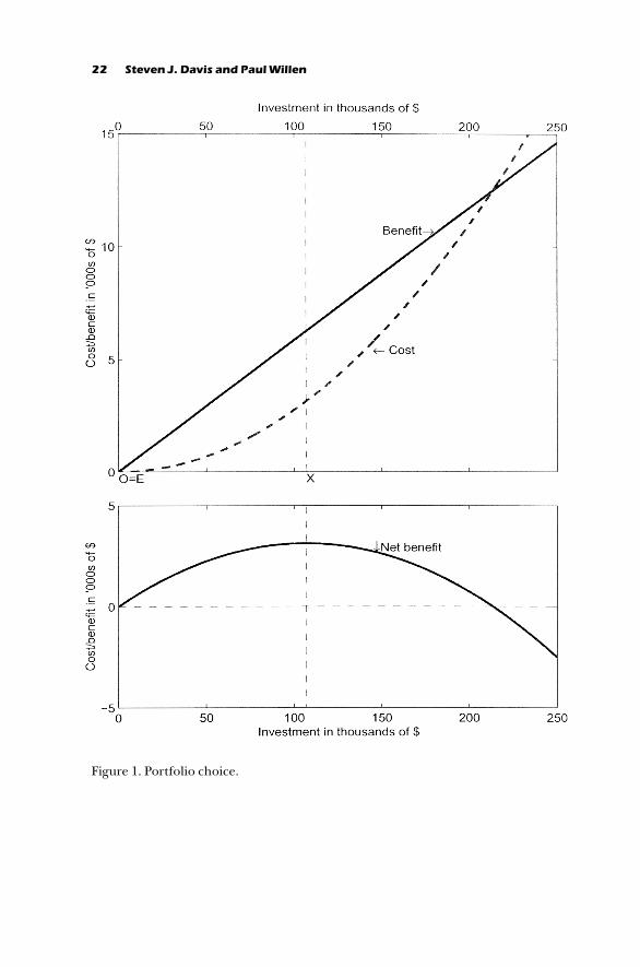
Let PVLR stand for the expected present value of lifetime earnings fromworking plus the present value of lifetime excess returns on risky assets.Investing in risky assets increases PVLR and thus the expected amount aninvestor can consume over her life cycle. In this sense, investing in riskyassets increases wealth. The solid line in Figure ∞ shows this wealth measureas a function of investment in a risky asset with an excess return of ∫ percent-age points.

But every dollar of investment in risky assets also increases the risk of herconsumption, as mentioned above. The dashed line in the top panel ofFigure ∞ shows the cost of increased consumption variability as a function ofinvestment in a risky asset with a standard deviation of ∞∑ percent. Wemeasure the cost as the amount of wealth that the investor would forgo toeliminate the consumption variability caused by the additional risky assetholdings. Suppose, for example, that you invest $∞≠,≠≠≠ in risky assets, andthis increases the variability of your future consumption by ∞≠ percent. Tomeasure the cost of the added risk, we ask how much additional income youwould require to compensate for the ∞≠ percent increase in consumptionvariability. Note that the slope of the cost curve increases with investment—

22 Steven J. Davis and Paul Willen

Figure ∞. Portfolio choice.


in contrast to the slope of the benefit curve, which is constant. The more ofa particular risk an investor takes on, the less willing she becomes to take onyet more of that same risk.≥

Given this tradeoff between risk and return, how should an investorchoose the optimal level of the risky asset? To answer this question, observethat the net benefit of the risky asset equals the difference between the solidand dotted lines—that is, between the benefit of higher expected consump-tion and the cost of higher risk. The bottom panel of Figure ∞ shows the netdifference between cost and benefit as a function of the amount invested.To maximize utility, an investor chooses the amount that maximizes the netbenefit, point X in Figure ∞. We call the distance from point O to point X aninvestor’s ‘‘desired exposure’’ to the risky asset.

Investors differ by age, wealth level, risk aversion, occupation, region, andmany other characteristics. How do these things affect portfolio choice?They do not affect the benefit of risky asset investment—a dollar investmentin a risky asset increases PVLR by the same amount for all people who facethe same risk-free interest rate. They typically do affect the cost to an inves-tor of taking on the type of risk implied by investments in the risky asset. Todevelop this point, we first discuss how age, wealth, and risk aversion affectthe cost of risky asset holdings. We then consider the role of labor incomeuncertainty, especially as it relates to an investor’s occupation.

Risk aversion. Some people find risk highly unpleasant, so that they arewilling to forego a relatively large amount of wealth to eliminate a givenamount of risk. Hence, the cost curve is higher and steeper for investorswith greater risk aversion (see Figure ≤). As a consequence, desired ex-posure is lower, other things equal.

Age. Younger investors have more time to smooth income or wealthshocks, so the cost of income variability is lower for younger persons. Forexample, a dollar shock to wealth for an investor who only expects to live foranother year results in a dollar shock to consumption. By contrast, a dollarshock to wealth for an investor who expects to live for another forty yearsresults in a very small shock to consumption. Thus for old people the costcurve (the dashed line) is higher and ‘‘desired exposure’’ is lower. A shorterplanning horizon, because of more advanced age or other reasons, affectsportfolio choice in much the same way as greater risk aversion.

Wealth. The more wealth you have, the less overall effect a dollar shock toyour wealth has on your consumption. If you lose $∑≠,≠≠≠ on the stockmarket and you have a net worth of $∞≠≠ million, that is not so bad. But ifyou lose $∑≠,≠≠≠ on the stock market and you have a net worth of $∑≠,≠≠≠,that is a disaster. Thus the less wealth you have, the higher and more steeplysloped is the cost curve and the lower your desired exposure. Increasedwealth affects portfolio choice in a similar way to decreased risk aversion.

Figure ≤ shows portfolio choice for two investors, one with high risk


Figure ≤. Portfolio choice with high and low risk aversion (RA).


aversion and the other with low risk aversion. The picture would look thesame if we compared high age and low age or low wealth and high wealth.

Risky Labor Income

The focus of this chapter is on risky labor income, particularly labor incomerisk tied to a worker’s occupation. How does the presence of risky laborincome affect portfolio choice? Unlike risk aversion, age, and wealth, riskylabor income does not change the shape of the cost curve. Rather, riskylabor income changes its location.

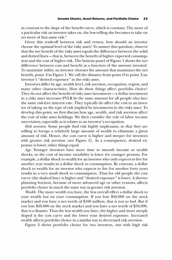
Consider the following example. Suppose an investor works for Ford. Sup-pose she knows that the price of Honda stock is negatively correlated withher labor income. When things go well for Honda—sales of Odyssey mini-vans increase, for example—Ford sales drop and bonuses shrink. Whenthings go poorly for Honda—the original Odyssey minivan was somethingof a dud—Ford sales increase and bonuses increase. Suppose she investssome money in Honda. When things go poorly at Ford (and well at Honda),her wealth and consumption fall by less than they would without the invest-ment in Honda. When things go well at Ford (and badly at Honda), herwealth and consumption increase by less than they would without the invest-ment in Honda. What has happened here? For the Ford employee, aninvestment in the risky Honda asset actually reduces the variability of herconsumption! Figure ≥ illustrates this graphically. The benefit of investingin a risky asset is still the same as before, but now the cost curve initiallyslopes down as she invests.

In the preceding example, our investor can increase her wealth and lowerher risk at the same time. This seems like a free lunch, and it is, but only upto a point. Since her exposure to Ford risk is fixed (determined by heremployment situation) the effects of added exposure to Honda risk even-tually swamp the reduction in Ford risk as she adopts larger positions in therisky Honda asset. Her net benefit is maximized at point X. To sum up,negative correlation between returns and labor income shifts the cost curvedown and to the right.

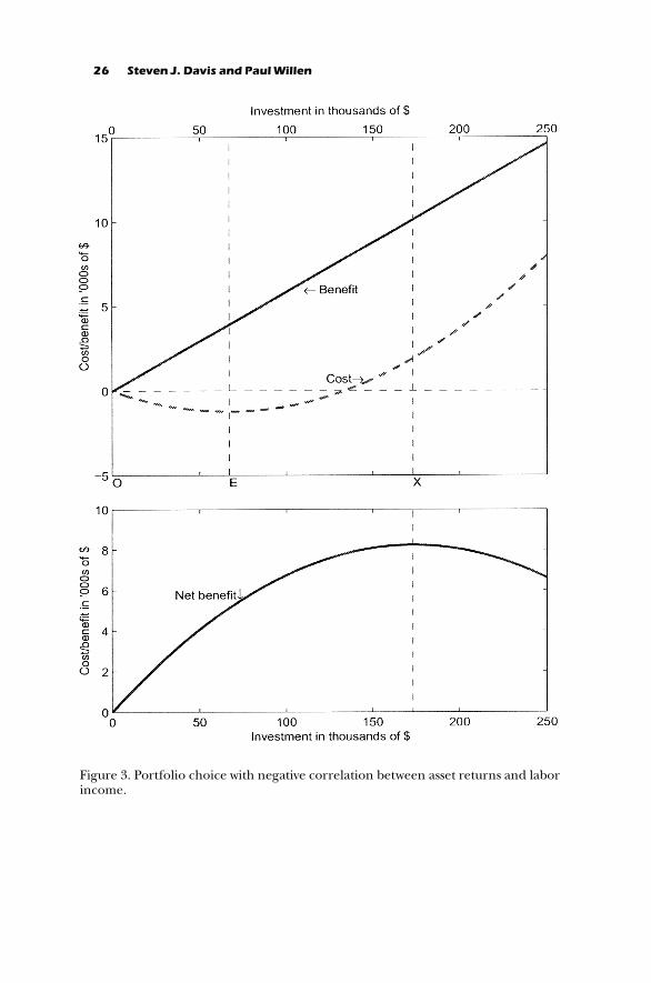
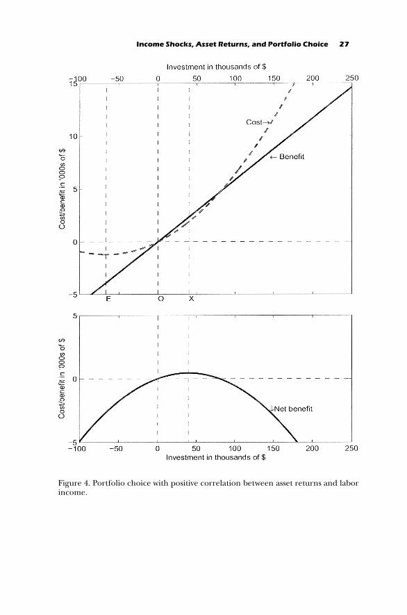
One can make a related argument for an investor who has labor incomethat is positively correlated with the returns on a risky asset. For example, aHonda employee may find that, by taking a short position in Honda stock,she can reduce the variability of her total income. But for any long positionthe cost is higher than it would be if she had no risky labor income at all, orrisky labor income that was uncorrelated with the returns on Honda stock.Figure ∂ illustrates this situation graphically. By taking a short position—that is, moving to the left of point O,—our investor sees her risk fall. But incontrast to the case of negative correlation in Figure ≥, now her benefit fallsas well. And for any positive investment the cost curve will be higher than itwould be in the absence of labor income risk.


Figure ≥. Portfolio choice with negative correlation between asset returns and laborincome.


Figure ∂. Portfolio choice with positive correlation between asset returns and laborincome.


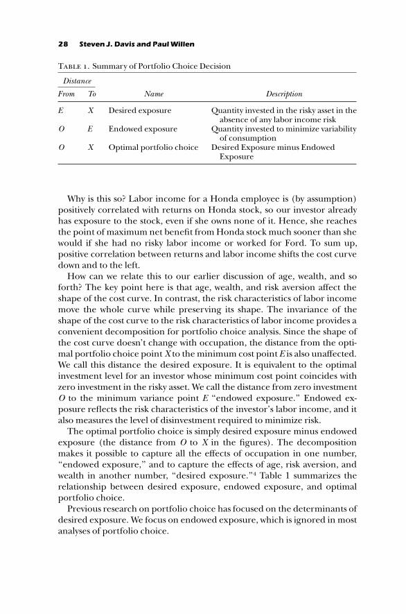
Table 1. Summary of Portfolio Choice Decision

Distance

From To Name Description

E X Desired exposure Quantity invested in the risky asset in theabsence of any labor income risk

O E Endowed exposure Quantity invested to minimize variabilityof consumption

O X Optimal portfolio choice Desired Exposure minus EndowedExposure

Why is this so? Labor income for a Honda employee is (by assumption)positively correlated with returns on Honda stock, so our investor alreadyhas exposure to the stock, even if she owns none of it. Hence, she reachesthe point of maximum net benefit from Honda stock much sooner than shewould if she had no risky labor income or worked for Ford. To sum up,positive correlation between returns and labor income shifts the cost curvedown and to the left.

How can we relate this to our earlier discussion of age, wealth, and soforth? The key point here is that age, wealth, and risk aversion affect theshape of the cost curve. In contrast, the risk characteristics of labor incomemove the whole curve while preserving its shape. The invariance of theshape of the cost curve to the risk characteristics of labor income provides aconvenient decomposition for portfolio choice analysis. Since the shape ofthe cost curve doesn’t change with occupation, the distance from the opti-mal portfolio choice point X to the minimum cost point E is also unaffected.We call this distance the desired exposure. It is equivalent to the optimalinvestment level for an investor whose minimum cost point coincides withzero investment in the risky asset. We call the distance from zero investmentO to the minimum variance point E ‘‘endowed exposure.’’ Endowed ex-posure reflects the risk characteristics of the investor’s labor income, and italso measures the level of disinvestment required to minimize risk.

The optimal portfolio choice is simply desired exposure minus endowedexposure (the distance from O to X in the figures). The decompositionmakes it possible to capture all the effects of occupation in one number,‘‘endowed exposure,’’ and to capture the effects of age, risk aversion, andwealth in another number, ‘‘desired exposure.’’∂ Table ∞ summarizes therelationship between desired exposure, endowed exposure, and optimalportfolio choice.

Previous research on portfolio choice has focused on the determinants ofdesired exposure. We focus on endowed exposure, which is ignored in mostanalyses of portfolio choice.


Measuring Endowed Exposure

The magnitude of an investor’s endowed exposure to a risky asset dependson three things:

Correlation. As we have discussed already, the higher the correlation, thehigher is endowed exposure.

Variability of income. The higher the variability of income, all else equal, thehigher is endowed exposure. Why? Return to our example. If you work forFord and your compensation is well insulated from the ups and downs ofFord’s fortunes, then the effect of a shock to Ford on your income will bevery small. Even if the correlation between Ford stock returns and yourincome is high, the potential for risk reduction is low, because you simplydon’t have very much risk to begin with.

Persistence. An investor’s lifetime consumption possibilities, as we alreadynoted, depend on the present value of her lifetime resources. A shock tolabor income obviously affects current labor income, but current labor in-come is typically only a small part of the present value of lifetime resources.In general, a shock to labor income today also conveys information about fu-ture labor income, and thus may have a large impact on lifetime resources.Consider a Ford employee who gets a reduced bonus because of poor salesone year. From a life cycle perspective, the reduced income this year is not soimportant. And if she expects the company to rebound quickly, this shockwill have little impact on her PVLR or her consumption. We call this a shockof low persistence. But if the reduced bonus presages major long-term cut-backs at the company, her lifetime resources may decline sharply—we callthis a shock of high persistence. The more persistent the shock, the more theshock affects PVLR and consumption, and the higher the endowed ex-posure to a given shock.

Persistence also depends on the retirement horizon. If a worker is onlyone year from retirement, a shock to income can only affect current in-come—so all shocks are of low persistence. Because of this horizon effect,labor income shocks effectively become less persistent as an investor ages.

When we actually go to the data below we measure persistence as theshock to the present value of lifetime resources of a dollar shock to laborincome this year. If a shock to labor income is highly persistent, then futurelabor income will be significantly affected and PVLR will change consid-erably—often by as much ≤≠ times the shock to current income. By contrast,if a shock to labor income is of low persistence, then future labor incomewon’t be greatly affected and PVLR will change by only a small amount.

To measure endowed exposure, therefore, we need to measure threethings: the variability of income shocks, the persistence of those shocks, andthe correlation of labor income shocks with stock returns or other riskyassets under consideration.


Multiple Risky Assets

So far, we have considered an investor investing in only one risky financialasset. In reality, investors have tens of thousands of risky financial assets tochoose from, from stocks in tiny start-up companies to mutual funds that tryto mimic the entire universe of stocks in the U.S. How can we analyze thesefinancial decisions? In the absence of labor income risk, this decision isactually remarkably simple. Consider two investors who have different levelsof risk aversion and no labor income risk. Using methods described above,we can calculate their optimal portfolios for each asset separately. For eachasset, the cost of risk curve will be higher for the more risk averse investor.Conveniently, the difference in costs across agents will be the same for eachasset—which means that the relative investment in any two stocks will be thesame—the ratio of shares held of Ford and Honda stock will be the same forall investors. This means that all investors will hold portfolios with identicalweights on individual stocks and mutual funds. This drastic simplification ofthe portfolio problem is known as the principle of two-fund separation, be-cause it says that a single mutual fund with the correct weights will enable allinvestors to implement optimal financial plans using just the mutual fundand a riskless bond.

When we add occupational or other sources of labor income risk, theprinciple of two-fund separation breaks down. Why? The key to two-fundseparation is that risk aversion, age, and wealth affect demand for all assetsby the same amount—they change the shape of the cost curve for everyasset in the same way. But labor income risk changes the location of the costcurve for each investor in a potentially different way. To return to our exam-ple, for a Ford employee, labor income risk moves her Ford cost curve to theleft and her Honda cost curve to the right—whereas for a Honda employee,labor income risk moves her Ford cost curve to the right and her Honda costcurve to the left. The ratio of holdings of Honda and Ford stock will nolonger, in general, be the same for different investors.

Limitations of Our Approach

Our approach makes many assumptions about life cycle portfolio choice. Itallows for unlimited borrowing of the riskless asset and unlimited short-salesof the risky asset. Short-sale restrictions on risky assets can be treated with-out great difficulty, but a proper treatment of borrowing constraints for theriskless asset complicates the analysis greatly in a many-period setting. Ourapproach also requires certain assumptions about the utility function andthe time series processes for labor income and asset returns, which allow usto consider each period separately. In other words, investors do not need toworry about the effects of their current choices on their choice sets in future


periods. (A mathematical treatment of these issues appears in Davis andWillen ≤≠≠≠b.)

Occuaption-Level Earnings Innovations

The chief empirical requirements of our approach are measures of (∞) cor-relation between labor income shocks and asset returns, (≤) variability ofincome shocks, and (≥) persistence of income shocks. It is interesting thatasset returns have received substantial attention from financial researchers,but only a handful of scholars have investigated their correlation with laboror proprietary business income. One such study, by Campbell et al. (∞ΩΩΩ),considers the correlation between aggregate equity returns and the perma-nent component of household income for three education groups. A sec-ond, by Davis and Willen (≤≠≠≠a), uses a synthetic panel to create demo-graphic groups defined by sex, educational attainment, and birth cohort.Although they use rather different empirical designs, both of these studiesfind that the correlation between labor income shocks and equity returnsrises with education. Heaton and Lucas (≤≠≠≠) emphasize a positive correla-tion between equity returns and the income of self-employed persons.∑

Whereas prior studies have relied on panel data sets or synthetic panelsconstructed from repeated cross sections as the basis for analysis, here wepursue a somewhat different empirical approach. In particular, we rely onthe repeated cross-section structure of the Current Population Survey toextract mean occupation-level income shocks, while controlling for a hostof observable worker characteristics. We then focus our empirical investiga-tion on the properties of the occupation-level shocks and their correlationwith asset returns.

Data Sources and Definitions

The Current Population Survey (CPS) randomly samples about ∏≠,≠≠≠ U.S.households every month. Among other items, the survey inquires aboutlabor earnings, employment status, hours worked, educational attainment,occupation, and demographic characteristics for each household member.The Annual Demographic Files in the March CPS contain individual dataon these items for the previous calendar year. Using the CPS March files, weestimate occupation-level components of individual annual earnings from∞Ω∏π to ∞ΩΩ∂.

To compute annual earnings, we use CPS data on wage and salary workersin the private and public sectors who were ≤≥ to ∑Ω years old in the earningsyear. Excluded from the earnings calculations are unincorporated self-employed persons, though we do include self-employment and farm in-come for persons who were mainly wage and salary workers. The sample is


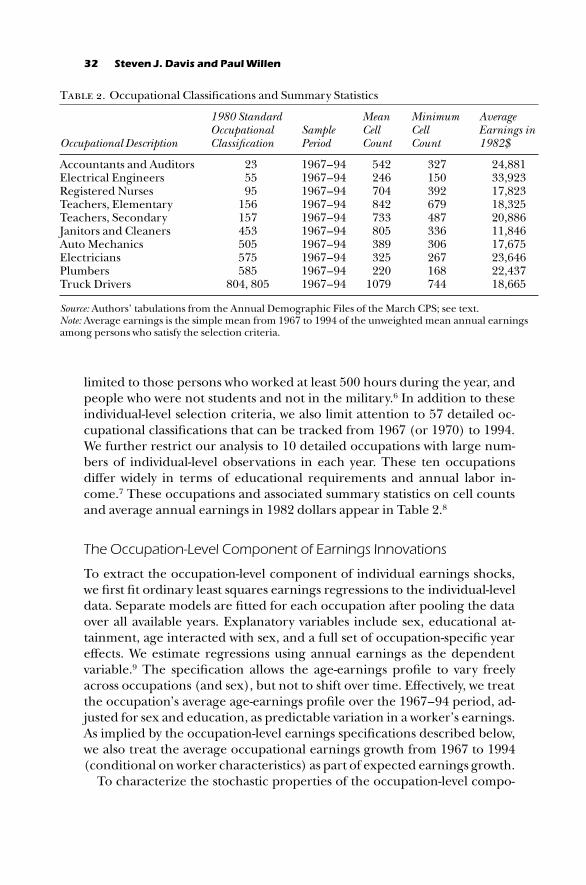
Table 2. Occupational Classifications and Summary Statistics

Occupational Description

∞Ω∫≠ StandardOccupationalClassification

SamplePeriod

MeanCellCount

MinimumCellCount

AverageEarnings in∞Ω∫≤$

Accountants and Auditors ≤≥ ∞Ω∏π–Ω∂ ∑∂≤ ≥≤π ≤∂,∫∫∞Electrical Engineers ∑∑ ∞Ω∏π–Ω∂ ≤∂∏ ∞∑≠ ≥≥,Ω≤≥Registered Nurses Ω∑ ∞Ω∏π–Ω∂ π≠∂ ≥Ω≤ ∞π,∫≤≥Teachers, Elementary ∞∑∏ ∞Ω∏π–Ω∂ ∫∂≤ ∏πΩ ∞∫,≥≤∑Teachers, Secondary ∞∑π ∞Ω∏π–Ω∂ π≥≥ ∂∫π ≤≠,∫∫∏Janitors and Cleaners ∂∑≥ ∞Ω∏π–Ω∂ ∫≠∑ ≥≥∏ ∞∞,∫∂∏Auto Mechanics ∑≠∑ ∞Ω∏π–Ω∂ ≥∫Ω ≥≠∏ ∞π,∏π∑Electricians ∑π∑ ∞Ω∏π–Ω∂ ≥≤∑ ≤∏π ≤≥,∏∂∏Plumbers ∑∫∑ ∞Ω∏π–Ω∂ ≤≤≠ ∞∏∫ ≤≤,∂≥πTruck Drivers ∫≠∂, ∫≠∑ ∞Ω∏π–Ω∂ ∞≠πΩ π∂∂ ∞∫,∏∏∑

Source: Authors’ tabulations from the Annual Demographic Files of the March CPS; see text.Note: Average earnings is the simple mean from ∞Ω∏π to ∞ΩΩ∂ of the unweighted mean annual earningsamong persons who satisfy the selection criteria.

limited to those persons who worked at least ∑≠≠ hours during the year, andpeople who were not students and not in the military.∏ In addition to theseindividual-level selection criteria, we also limit attention to ∑π detailed oc-cupational classifications that can be tracked from ∞Ω∏π (or ∞Ωπ≠) to ∞ΩΩ∂.We further restrict our analysis to ∞≠ detailed occupations with large num-bers of individual-level observations in each year. These ten occupationsdiffer widely in terms of educational requirements and annual labor in-come.π These occupations and associated summary statistics on cell countsand average annual earnings in ∞Ω∫≤ dollars appear in Table ≤.∫

The Occupation-Level Component of Earnings Innovations

To extract the occupation-level component of individual earnings shocks,we first fit ordinary least squares earnings regressions to the individual-leveldata. Separate models are fitted for each occupation after pooling the dataover all available years. Explanatory variables include sex, educational at-tainment, age interacted with sex, and a full set of occupation-specific yeareffects. We estimate regressions using annual earnings as the dependentvariable.Ω The specification allows the age-earnings profile to vary freelyacross occupations (and sex), but not to shift over time. Effectively, we treatthe occupation’s average age-earnings profile over the ∞Ω∏π–Ω∂ period, ad-justed for sex and education, as predictable variation in a worker’s earnings.As implied by the occupation-level earnings specifications described below,we also treat the average occupational earnings growth from ∞Ω∏π to ∞ΩΩ∂(conditional on worker characteristics) as part of expected earnings growth.

To characterize the stochastic properties of the occupation-level compo-


nent of individual earnings shocks, we fit autoregressive moving average(ARMA) models to the first-differenced values of the occupation-year ef-fects. We denote the occupation-year effects estimated in the first-stageearnings regressions as et, t = ∞Ω∏π, ∞Ω∏∫, . . . , ∞ΩΩ∂. Then we fit second-order moving average processes, following MaCurdy (∞Ω∫≤), who uses paneldata on individuals, and Davis and Willen (≤≠≠≠a), who use synthetic paneldata for demographic groups:

qet = a + ht + c∞ ht–∞ + c≤ ht–≤ .(∞)

Here ht denotes the time-t innovation to the occupation-level component ofindividual earnings shocks. These innovations and their correlation withasset returns are the main focus of the empirical investigation and theapplied portfolio analysis below.∞≠

Magnitude and Persistence of Earnings Innovations

The standard deviation of ht in equation (∞) quantifies the magnitude ofinnovations to the occupation-level component of individual earnings. Asdescribed earlier, we measure persistence as the shock to PVLR of a dollarshock to income. We refer to this persistence measure as the present valuemultiplier (PVM). The magnitude of the PVM depends on the persistenceof h (a function of c∞ and c≤), the risk-free rate of interest, and the numberof years remaining until retirement. By combining these elements, we caneasily calculate the magnitude of a typical shock to PVLR at a given age. Themagnitude of this shock declines with age, because fewer years remain untilretirement.

Table ≥ reports the present value multipliers on the occupation-levelearnings shocks at ages ≥≠ and ∑≠, assuming a real discount rate of ≤.∑ per-cent per year and retirement after age ∑Ω. To illustrate the calculation of theshock to PVLR implied by an occupation-level income innovation, considerthe example of the accountants and auditors occupation at age ≥≠. Accord-ing to Table ≥, the standard deviation of innovations to the occupation-levelcomponent of earnings is $∞,≠∫≠, or ∂.≥ percent of annual earnings. At age≥≠, the present value multiplier on this innovation is ≤≠.≠, so that the im-plied impact on PVLR amounts to ∞≠∫≠ (≤≠.≠) = $≤∞,∏≠≠. This figure is ∫πpercent of the average annual earnings for accountants and auditors re-ported in Table ≤. These calculations show that occupation-level earningsinnovations are of modest size, but the implied effects on the present valueof lifetime earnings are not.

Occupations differ in terms of magnitude and persistence of occupation-level earnings innovations. The standard deviation of the occupation-levelinnovations ranges from ≤.Ω to ∏.Ω percent of annual earnings. Plumbershave the most volatile occupation-level earnings component in both dollar


Tab

le 3

.Se

lect

ed S

tatis

tics f

or th

e O

ccup

atio

nal C

ompo

nent

of I

ndiv

idua

l Ear

ning

s, ∞

Ω∏∫–

∞ΩΩ∂

Occ

upati

onal D

escr

ipti

onSta

ndard

Dev

iati

onof

Labo

r In

com

e Shoc

ksSta

ndard

Dev

iati

onas

% o

f In

com

e

Pre

sen

t Valu

e M

ult

ipli

er a

t:

Age

≥≠

Age

∑≠

Acc

ount

ants

and

Aud

itors

∞≠∫≠

∂.≥∂

≤≠.≠

∫.≥

Ele

ctri

cal E

ngin

eers

∞≤∫≥

≥.π∫

∏.∫

≥.∂

Reg

iste

red

Nur

ses

∂∂∏

≤.∑≠

∂≠.≤

∞∑.Ω

Ele

men

tary

Sch

ool T

each

ers

∑≤∑

≤.∫∏

≤π.≤

∞∞.≠

Seco

ndar

y Sc

hool

Tea

cher

s∏≥

π≥.

≠∑≤≤

.∑Ω.

∂Ja

nito

rs a

nd C

lean

ers

∑∫≥

∂.Ω≤

∞≥.≥

∑.∫

Aut

o M

echa

nics

π∞∂

∂.≠∂

∞∫.Ω

∫.≠

Ele

ctri

cian

sΩ∑

∞∂.

≠≤∞≥

.≤∏.

∞Pl

umbe

rs∞∂

∑≥∏.

∂∫∞≤

.∫∑.

πT

ruck

Dri

vers

πΩ≠

∂.≤≥

∞∫.∑

∫.≠

Sou

rce:

Aut

hors

’ cal

cula

tions

, CPS

dat

a.N

otes

: For

eac

h oc

cupa

tion,

a se

cond

-ord

er m

ovin

g av

erag

e pr

oces

s is fi

t to

the

occu

patio

nal c

ompo

nent

of i

ndiv

idua

l ann

ual

earn

ings

in ∞

Ω∫≤

dolla

rs. T

he m

ovin

g av

erag

e pr

oces

s is e

stim

ated

by

(con

ditio

nal)

non

linea

r le

ast s

quar

es. S

ee D

avis

and

Will

en(≤

≠≠≠b

) fo

r an

exp

lana

tion

of h

ow th

e oc

cupa

tiona

l com

pone

nt o

f ind

ivid

ual e

arni

ngs i

s ide

ntifi

ed. P

rese

nt v

alue

mul

tiplie

rsco

mpu

ted

usin

g a

real

dis

coun

t rat

e of

≤.∑

per

cent

per

yea

r an

d as

sum

ing

retir

emen

t aft

er a

ge ∑

Ω.


and percentage terms, while registered nurses and elementary school teach-ers have the least volatile. Likewise, the present value multiplier at age ≥≠ is∏.∫ for plumbers and ∂≠.≤ for registered nurses. These two occupations areoutliers in terms of persistence. For the other occupations, the present valuemultipliers at age ≥≠ range from ∞≥ to ≤π. The last two columns in Table ≥show how the present value multiplier declines between ages ≥≠ and ∑≠,given the assumptions about discounting and retirement. The age-∑≠ multi-pliers are fairly sensitive to alternative assumptions about retirement age,but the basic point is not. As workers near retirement, earnings innovationshave smaller and smaller effects on lifetime resources.

Correlation Between Occupation-Level IncomeInnovations and Asset Returns

To investigate the correlation between occupation-level earnings innova-tions and aggregate equity returns, we next regress ht from equation (∞) onthe realized market rate of return during period t. Recall that we can use theslope coefficient in an ordinary least squares (OLS) regression of y on x togenerate an estimate of the correlation of x with y. Hence, we can usestandard regression methods to quantify the correlation between incomeshocks and equity returns and to test whether the relationship is statisticallysignificant.

Correlation with Aggregate Equity Returns

We find little evidence that occupation-level income innovations and aggre-gate equity returns are linearly related in annual data over the period ∞Ω∏∫to ∞ΩΩ∂. None of the ten occupations considered evinces a statistically signif-icant relationship between income innovations and returns on the value-weighted market portfolio (in regressions not detailed here).∞∞ As a check,we also considered the returns on several other broad-based equity indexes:the S&P ∑≠≠, the New York Stock Exchange, the Wilshire ∑≠≠≠, and a value-weighted composite of the New York Stock Exchange, American Stock Ex-change and NASDAQ. For each measure, we see the same pattern of little orno evidence for a relationship between occupation-level income innova-tions and contemporaneous aggregate equity returns.

This result is puzzling from the vantage point of standard economic theo-ries of growth, fluctuations, and asset pricing. Equilibrium models that obeystandard asset-pricing relationships and embed a conventional specificationof the aggregate production technology imply a high positive correlationbetween aggregate equity returns and shocks to labor income.∞≤ While wenote this puzzle here, it is not necessary to resolve it to pursue the remainderof our agenda.


Other Asset Return Measures

We also investigate the correlation between occupation-level income inno-vations and the returns on long-term government bonds and other assets.Bond returns are significantly correlated with income innovations for afew occupations. In most cases, bonds account for a greater fraction ofoccupation-level income innovations when the returns are measured innominal terms.

We examine two additional types of assets which might be highly corre-lated with labor income shocks. First, we sought to construct industry equityportfolios that respond sensitively to labor income shocks in particular oc-cupations. For example, demand shocks in the construction sector inducea positive correlation between equity returns in Construction industries(SICs ∞∑, ∞∏, ∞π) and occupation-level income innovations for ElectricalEngineers, Electricians, and Plumbers. More generally, industry-level de-mand shocks and factor-neutral technology shocks impart a positive corre-lation between returns on industry equity and occupation-level incomeinnovations.

However, prior reasoning alone cannot determine the sign, let alone themagnitude, of the correlation between industry equity returns and laborincome innovations for industry workers. For example, labor-saving tech-nological improvements in construction activity might be good for share-holders but bad for the earnings of Electricians and Plumbers. As anotherexample, the deregulation of the trucking industry during the ∞Ωπ≠s andearly ∞Ω∫≠s was bad news for many truck drivers (Rose, ∞Ω∫π) but good newsfor many trucking firms (Keeler, ∞Ω∫Ω). The basic point is that factor-biasedtechnology shifts (construction example) and rent shifting between ownersand workers (trucking example) impart a negative correlation betweenindustry-level equity returns and occupation-level income innovations.

Clearly the relationship between industry-level equity portfolios and la-bor income shocks is very much an empirical issue. Furthermore, if the mixof underlying shocks and economic response mechanisms changes overtime, the correlation between industry-level equity returns and occupation-level income innovations is likely to change. The weight of this concern isalso largely an empirical issue. No single study can definitively settle theseempirical issues, so our results in this regard are best viewed as one install-ment in a broader empirical inquiry.

We construct industry portfolios using firm-level equity returns and mar-ket values in the Center for Research in Security Prices (CRSP) database.For each occupation (except Janitors and Cleaners) we identify one or moreindustries that account for a large fraction of the occupation’s employment.In some cases, we had to omit natural SIC counterparts for particular oc-cupations, because CRSP contains no firm-level observations during part ofthe sample period.∞≥ Int he end, the SIC industry groups listed in Table ∂ are

Income Shocks, Asset Returns, and Portfolio Choice 37T

able

4.

Ass

et R

etur

n M

easu

res,

Defi

nitio

ns, a

nd S

umm

ary

Stat

istic

s

Vari

abl

eN

am

eD

escr

ipti

on

Mea

n A

nn

ual

Ret

urn

(%

),∞Ω∏∫

–Ω∂

Sta

ndard

Dev

iati

on o

fA

nn

ual R

etu

rnO

ccu

pati

on M

atc

h

SMB

Fam

a-Fr

ench

Siz

e Po

rtfo

lio, S

mal

l-Big

≠.≤

∞∑.∑

All

HM

LFa

ma-

Fren

ch B

ook-

to-M

arke

t Por

tfol

io, V

alue

—G

row

thSt

ocks

∑.Ω

∞≤.Ω

All

Bon

dsN

omin

al R

etur

n on

∞≠-

Year

Con

stan

t Mat

urit

y U

.S. G

ov-

ernm

ent B

onds

∫.∑

∞≠.∞

All

Aut

osR

eal R

etur

n on

SIC

≥π∞

(A

uto

Mfg

.)∏.

∂≤∑

.≠A

uto

Mec

hani

csE

lmac

hR

eal R

etur

n on

SIC

≥∏

(Ele

ctri

cal M

achi

nery

Man

ufac

turi

ng)

∑.∫

≤∞.∂

Ele

ctri

cal E

ngin

eers

Bui

ldR

eal R

etur

n on

SIC

s ∞∑,

∞∏,

∞π

(Con

stru

ctio

n)≥.

≤≤π

.∫E

lec.

Eng

s., E

lect

rici

ans,

Plum

bers

Frei

ght

Rea

l Ret

urn

on S

IC ∂

≤ an

d ∂π

≤, e

x. ∂

π≤∑

(Fre

ight

Tra

ns-

port

by

Roa

d)∏.

∂≤π

.∫T

ruck

Dri

vers

Tech

nica

lR

eal R

etur

n on

SIC

s ∫π∞

and

π≥≥

∏ (E

ngin

eeri

ng, A

rchi

tec-

tura

l and

Tec

hnic

al S

ervi

ces)

∫.∞

≥∞.Ω

Ele

ctri

cal E

ngin

eers

Edu

catio

nR

eal R

etur

n on

SIC

s ∫≤,

ex.

∫≤≥

, and

∫≥≥

(E

duca

tion

Ser-

vice

s)∏.

∂≥π

.∞E

lem

enta

ry a

nd S

econ

d-ar

y Te

ache

rsH

ealth

Rea

l Ret

urn

on S

IC ∫

≠ (M

edic

al, D

enta

l and

Hea

lthSe

rvic

es)

∞≤.∫

≥π.∞

Reg

iste

red

Nur

ses

Util

ity

Rea

l Ret

urn

on S

ICs ∂

∏ an

d ∂Ω

, ex.

∂Ω∑

(E

lect

rici

ty, G

as,

Stea

m, W

ater

Wor

ks)

∑.∂

∞∑.∫

Ele

ctri

cal E

ngin

eers

,E

lect

rici

ans,

Plu

mbe

rsFi

nanc

eR

eal R

etur

n on

SIC

s ∏≤,

∏π

(Inv

estm

ent B

anki

ng, S

e-cu

ritie

s Mar

kets

, Exc

hang

es)

π.Ω

∞Ω.∫

Acc

ount

ants

and

Aud

itors

Sou

rces

: Ret

urns

dat

a fo

r th

e SM

B a

nd H

ML

por

tfol

ios t

aken

from

»web

.mit.

edu

/kf

renc

h/

ww

w/

data

.libr

ary.

htm

l…; s

ee a

lso

Fam

a an

d Fr

ench

(∞Ω

Ω≥)

for

cons

truc

tion

of th

ese

port

folio

s. R

etur

ns d

ata

on B

onds

from

Cen

ter

for

Res

earc

h in

Sec

urit

y Pr

ices

; all

indu

stry

-leve

l ret

urn

seri

es c

onst

ruct

ed fr

omva

lue-

wei

ghte

d po

rtfo

lios o

f firm

-leve

l equ

ity

retu

rns i

n th

e C

ente

r fo

r R

esea

rch

in S

ecur

ity

Pric

es d

atab

ase;

see

Dav

is a

nd W

illen

(≤≠

≠≠a)

.N

otes

: Nom

inal

ret

urns

for

the

indu

stry

-leve

l mea

sure

s con

vert

ed to

rea

l ret

urns

usi

ng th

e G

DP

defl

ator

for

pers

onal

con

sum

ptio

n ex

pend

iture

s. D

ata

poin

ts m

issi

ng fo

r H

ealth

in ∞

Ω∏∫

and

for

Tech

nica

l in

∞Ω∫π

and

∞Ω∫

∫. L

ast c

olum

n lis

ts th

e oc

cupa

tion

for

whi

ch th

e re

turn

s mea

sure

is u

sed

as a

regr

esso

r.


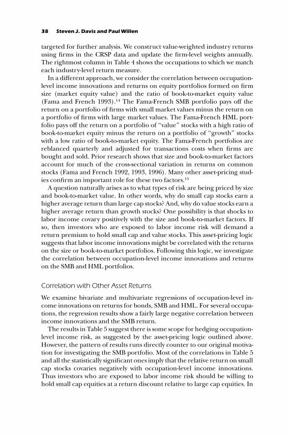
targeted for further analysis. We construct value-weighted industry returnsusing firms in the CRSP data and update the firm-level weights annually.The rightmost column in Table ∂ shows the occupations to which we matcheach industry-level return measure.

In a different approach, we consider the correlation between occupation-level income innovations and returns on equity portfolios formed on firmsize (market equity value) and the ratio of book-to-market equity value(Fama and French ∞ΩΩ≥).∞∂ The Fama-French SMB portfolio pays off thereturn on a portfolio of firms with small market values minus the return ona portfolio of firms with large market values. The Fama-French HML port-folio pays off the return on a portfolio of ‘‘value’’ stocks with a high ratio ofbook-to-market equity minus the return on a portfolio of ‘‘growth’’ stockswith a low ratio of book-to-market equity. The Fama-French portfolios arereblanced quarterly and adjusted for transactions costs when firms arebought and sold. Prior research shows that size and book-to-market factorsaccount for much of the cross-sectional variation in returns on commonstocks (Fama and French ∞ΩΩ≤, ∞ΩΩ≥, ∞ΩΩ∏). Many other asset-pricing stud-ies confirm an important role for these two factors.∞∑

A question naturally arises as to what types of risk are being priced by sizeand book-to-market value. In other words, why do small cap stocks earn ahigher average return than large cap stocks? And, why do value stocks earn ahigher average return than growth stocks? One possibility is that shocks tolabor income covary positively with the size and book-to-market factors. Ifso, then investors who are exposed to labor income risk will demand areturn premium to hold small cap and value stocks. This asset-pricing logicsuggests that labor income innovations might be correlated with the returnson the size or book-to-market portfolios. Following this logic, we investigatethe correlation between occupation-level income innovations and returnson the SMB and HML portfolios.

Correlation with Other Asset Returns

We examine bivariate and multivariate regressions of occupation-level in-come innovations on returns for bonds, SMB and HML. For several occupa-tions, the regression results show a fairly large negative correlation betweenincome innovations and the SMB return.

The results in Table ∑ suggest there is some scope for hedging occupation-level income risk, as suggested by the asset-pricing logic outlined above.However, the pattern of results runs directly counter to our original motiva-tion for investigating the SMB portfolio. Most of the correlations in Table ∑and all the statistically significant ones imply that the relative return on smallcap stocks covaries negatively with occupation-level income innovations.Thus investors who are exposed to labor income risk should be willing tohold small cap equities at a return discount relative to large cap equities. In


Table 5. Determinants of Endowed Exposure for SMB Portfolio, ∞Ω∏∫–Ω∂

Occupational Description CorrelationVariability(std. dev.)

PVM at Age≥≠

Accountants and Auditors –≠.≥π ∞≠∫≠ ≤≠.≠Electrical Engineers –≠.≥≥ ∞≤∫≥ ∏.∫Registered Nurses –≠.∞∂ ∂∂∏ ∂≠.≤Teachers, Elementary –≠.≥∏ ∑≤∑ ≤π.≤Teachers, Secondary –≠.≥Ω ∏≥π ≤≤.∑Janitors and Cleaners –≠.≥≤ ∑∫≥ ∞≥.≥Auto Mechanics –≠.∞≠ π∞∂ ∞∫.ΩElectricians ≠.≤≤ Ω∑∞ ∞≥.≤Plumbers –≠.≤∫ ∞∂∑≥ ∞≤.∫Truck Drivers ≠.≠≥ πΩ≠ ∞∫.∑

Source: Authors’ calculations; see text.Notes: All regressions estimated by ordinary least squares. For regression results, see Davis andWillen (≤≠≠≠b).

fact, the average return on small cap stocks is higher.∞∏ So, while the findingscan be useful for portfolio design purposes, they serve to heighten ratherthan resolve asset-pricing puzzles related to the return premium on smallcap stocks.

Life Cycle Portfolio Choice with Risky Labor Income: SomeExamples

We now solve the life cycle portfolio problem with risky labor income, draw-ing on the just presented empirical evidence to characterize the magnitude,persistence, and correlation properties of labor income shocks.

Preliminaries and Two-Fund Separation

Optimal portfolio allocations when asset returns and labor income areuncorrelated appear in Table ∏. The table considers three risky assets—market, size, and value portfolios—and uses a real risk-free return of ≥.∑percent per year. We do not impose short-sale constraints on risky assetholdings or restrictions on borrowing at the risk-free rate. Since two-fundseparation holds under these conditions, every investor has the same riskyasset portfolio shares, as shown in the top row. These shares depend on thejoint return distribution for the three assets, which we fit to the first twosample moments in the data. The table also displays optimal risky assetholdings at ages ∂≠ and ∏≠ for two occupations under various assumptionsabout relative risk aversion and expected returns.

We measure risk aversion using the Arrow-Pratt coefficient of relative riskaversion (RRA). To understand RRAs, consider the following experiment.


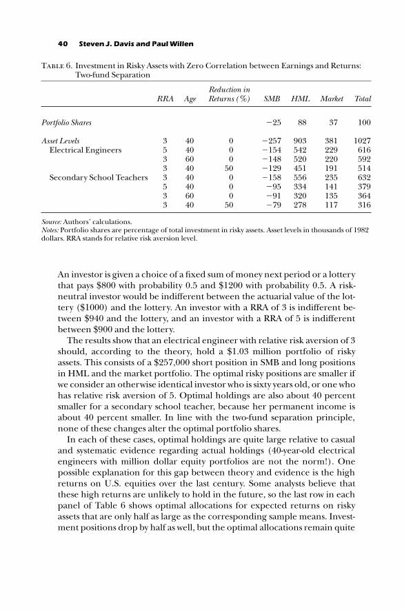
Table 6. Investment in Risky Assets with Zero Correlation between Earnings and Returns:Two-fund Separation

RRA AgeReduction inReturns (%) SMB HML Market Total

Portfolio Shares –≤∑ ∫∫ ≥π ∞≠≠

Asset Levels ≥ ∂≠ ≠ –≤∑π Ω≠≥ ≥∫∞ ∞≠≤πElectrical Engineers ∑ ∂≠ ≠ –∞∑∂ ∑∂≤ ≤≤Ω ∏∞∏

≥ ∏≠ ≠ –∞∂∫ ∑≤≠ ≤≤≠ ∑Ω≤≥ ∂≠ ∑≠ –∞≤Ω ∂∑∞ ∞Ω∞ ∑∞∂

Secondary School Teachers ≥ ∂≠ ≠ –∞∑∫ ∑∑∏ ≤≥∑ ∏≥≤∑ ∂≠ ≠ –Ω∑ ≥≥∂ ∞∂∞ ≥πΩ≥ ∏≠ ≠ –Ω∞ ≥≤≠ ∞≥∑ ≥∏∂≥ ∂≠ ∑≠ –πΩ ≤π∫ ∞∞π ≥∞∏

Source: Authors’ calculations.Notes: Portfolio shares are percentage of total investment in risky assets. Asset levels in thousands of ∞Ω∫≤dollars. RRA stands for relative risk aversion level.

An investor is given a choice of a fixed sum of money next period or a lotterythat pays $∫≠≠ with probability ≠.∑ and $∞≤≠≠ with probability ≠.∑. A risk-neutral investor would be indifferent between the actuarial value of the lot-tery ($∞≠≠≠) and the lottery. An investor with a RRA of ≥ is indifferent be-tween $Ω∂≠ and the lottery, and an investor with a RRA of ∑ is indifferentbetween $Ω≠≠ and the lottery.

The results show that an electrical engineer with relative risk aversion of ≥should, according to the theory, hold a $∞.≠≥ million portfolio of riskyassets. This consists of a $≤∑π,≠≠≠ short position in SMB and long positionsin HML and the market portfolio. The optimal risky positions are smaller ifwe consider an otherwise identical investor who is sixty years old, or one whohas relative risk aversion of ∑. Optimal holdings are also about ∂≠ percentsmaller for a secondary school teacher, because her permanent income isabout ∂≠ percent smaller. In line with the two-fund separation principle,none of these changes alter the optimal portfolio shares.

In each of these cases, optimal holdings are quite large relative to casualand systematic evidence regarding actual holdings (∂≠-year-old electricalengineers with million dollar equity portfolios are not the norm!). Onepossible explanation for this gap between theory and evidence is the highreturns on U.S. equities over the last century. Some analysts believe thatthese high returns are unlikely to hold in the future, so the last row in eachpanel of Table ∏ shows optimal allocations for expected returns on riskyassets that are only half as large as the corresponding sample means. Invest-ment positions drop by half as well, but the optimal allocations remain quite


large compared to observed holdings for the typical person. This portfoliopuzzle has received little attention in previous research because of thestrong proclivity to focus on portfolio shares and to disregard theoreticalimplications for the level of risky asset holdings.∞π

We believe that the resolution of this puzzle rests at least partly on theopportunity cost of investor funds. In computing the portfolio allocations inTable ∏, investors are allowed to borrow unlimited amounts at the risk-freeinterest rate. If, instead, investors must borrow at an interest rate that ap-proximates the expected return on risky assets, then the optimal risky assetposition is approximately zero when asset returns and labor income areuncorrelated. Many (potential) investors face an opportunity cost of fundsat least as great as the expected return on equities, so it is not surprising thathalf or more of all households have little or no holdings of risky financialassets.

Endowed Exposure and the Breakdown of Two-Fund Separation

Nonzero correlations between asset returns and labor income cause two-fund separation to break down in a particular way. To illustrate this point,Table π shows optimal allocations for seven occupations when we accountfor correlation with labor income shocks. Recall from above that optimalholdings in the zero-correlation case, ‘‘desired exposure,’’ depend only onrisk aversion, age, wealth, and asset returns. ‘‘Endowed exposure’’ gives therisky asset position implicit in the correlation between asset returns and theworker-investor’s labor income.

The results in Table ∑ above demonstrated that most occupational groupshave a negative endowed exposure to the SMB portfolio. As we explainedabove, the endowed exposure reflects the size and persistence of labor in-come innovations and their correlation with asset returns. Consequently,although income shocks for janitors and cleaners and electrical engineershave almost the same correlation with SMB, the endowed exposure of elec-trical engineers is much lower because their income shocks are more vari-able and more persistent.

To calculate an investor’s optimal portfolio, we simply subtract endowedexposure from desired exposure. Since endowed exposure is not propor-tional to desired exposure, two-fund separation fails. Other things equal,the bigger the endowed exposure the bigger the departure from the two-fund separation principle. Table ∫ illustrates this breakdown by showingoptimal portfolio shares under different assumptions about risk aversionand excess returns for each occupation that has a non-zero correlation withone or more of the assets. The base case uses sample average excess returnsand a relative risk aversion of ≥. Given these assumptions, the departuresfrom two-fund separation are modest. For example, the optimal shares for


Table 7. Endowed exposure, desired exposure and portfolio holdings

SBM HML Market Total

Accountants and Auditors Endowed Exposure –≥∏ ≠ ≠ –≥∏Desired Exposure –∞∫Ω ∏∏≤ ≤∫≠ π∑≥Portfolio position –∞∑≥ ∏∏≤ ≤∫≠ π∫Ω

Electrical Engineers Endowed Exposure –≤∫ ≠ ≠ –≤∫Desired Exposure –≤∑π Ω≠≥ ≥∫∞ ∞≠≤πPortfolio position –≤≤Ω Ω≠≥ ≥∫∞ ∞≠∑∑

Elementary School Teachers Endowed Exposure –∂≤ ≠ ≠ –∂≤Desired Exposure –∞≥Ω ∂∫∫ ≤≠∏ ∑∑∑Portfolio position –Ωπ ∂∫∫ ≤≠∏ ∑Ωπ

Secondary School Teachers Endowed Exposure –∑≤ ≠ ≠ –∑≤Desired Exposure –∞∑∫ ∑∑∏ ≤≥∑ ∏≥≤Portfolio position –∞≠∏ ∑∑∏ ≤≥∑ ∏∫∂

Janitors and Cleaners Endowed Exposure –∞≥ ≠ ≠ –∞≥Desired Exposure –Ω≠ ≥∞∑ ∞≥≥ ≥∑ΩPortfolio position –π∏ ≥∞∑ ∞≥≥ ≥π≤

Plumbers Endowed Exposure –∂∏ ≠ ≠ –∂∏Desired Exposure –∞π≠ ∑Ωπ ≤∑≤ ∏πΩPortfolio position –∞≤∂ ∑Ωπ ≤∑≤ π≤∑

Truck Drivers Endowed Exposure –≠ ∞∏ –≠ ∞∏Desired Exposure –∞∂∞ ∂Ωπ ≤∞≠ ∑∏∑Portfolio position –∞∂∞ ∂∫∞ ≤∞≠ ∑∑≠

Source: Authors’ calculations.Notes: Entries show endowed exposure, desired exposure and optimal portfolio position for indicatedrisky assets in thousands of ∞Ω∫≤$. Calculations assume a ∂≠-year-old investor who has a relative riskaversion of ≥.

electrical engineers never differ from the zero-correlation optimum bymore than three percentage points. For secondary school teachers, thetraditional zero-correlation portfolio understates SMB holdings by nine per-centage points.

Because these effects are small, a portfolio manager might be forgiven forignoring them. However, if one believes that high equity returns in recentdecades are an aberration, or that expected returns have declined in recentyears, then the effects of correlation on optimal portfolio shares becomemore important. As an example, the second line for each occupation inTable ∫ shows optimal portfolio shares when we set excess returns to one-half their sample averages. Recall that this change has no impact on theoptimal shares when two-fund separation holds. In particular, the optimalSMB share is –≤∑ percent under two-fund separation, regardless whetherwe scale down excess returns. This invariance result fails when we takecorrelation into account. As an example, the optimal SMB portfolio sharefor secondary school teachers is +≤ percent when excess returns are halftheir sample values and relative risk aversion is ∑. To understand this result,


Table 8. Risk Aversion, Excess Returns, and Optimal Portfolio Shares in the Case of ThreeRisky Assets

Reductionin Excess

Returns (%) RRA SMB HML Market

Accountants and Auditors ≠∑≠π∑

≥∑∑

–∞Ω–∫

∑

∫∂π∏∏π

≥∑≥≤≤∫

Electrical Engineers ≠∑≠π∑

≥∑∑

–≤≤–∞∑–∏

∫∏∫∞π∑

≥∏≥∂≥∞

Elementary School Teachers ≠∑≠π∑

≥∑∑

–∞∏≠

∞π

∫≤π≠∑∫

≥∑≥≠≤∑

Secondary School Teachers ≠∑≠π∑

≥∑∑

–∞∏≤

∞Ω

∫∞∏Ω∑π

≥∂≤Ω≤∂

Janitors and Cleaners ≠∑≠π∑

≥∑∑

–≤∞–∞∞–≠

∫∑∫∑π≠

≥∏≥≥≥≠

Plumbers ≠∑≠π∑

≥∑∑

–∞π–≤∞∂

∫≤π≤∏∞

≥∑≥≠≤∏

Truck Drivers ≠∑≠π∑

≥∑∑

–≤∏–≤∫–≥∞

∫∫∫π∫∑

≥∫∂∞∂∏

Source: Authors’ calculations.Notes: ‘‘Percent Reduction In Excess Returns’’ of ≠ means that expected returns on risky assets are set torealized sample values.A ∑≠ percent reduction means that the excess return (sample mean return minus a risk-free rate of≥.∑%) is set to half its sample value, and similarly for a π∑ percent reduction. RRA stands for relative riskaversion level. Entries in the last three columns show the percentage of risky financial asset holdings inthe indicated asset. All calculations assume an investor ∂≠ years old.

recall that the level of excess returns has no effect on ‘‘endowed exposure.’’So, as we reduce excess returns and hence desired exposure, the relative sizeof endowed exposure goes up.

Higher risk aversion has the same effect, and for much the same reason.Greater risk aversion lowers desired exposure but does not affect endowedexposure. The last line in each panel of Table ∫ shows optimal portfolioshares for the case of high risk aversion and low excess returns. In this case,the optimal portfolio shares sometimes differ substantially from the two-fund separation case. Based on traditional mean-variance analysis, a port-folio advisor would recommend a ≤∑ percent short position in SMB. Incontrast, the optimal position for secondary school teachers is a ∞π percentlong position in a plausible case that accounts for correlation between assetreturns and labor income.


Life Cycle Variation in Endowed Exposure

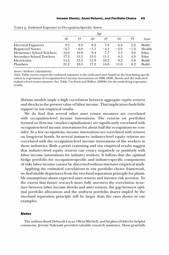
Endowed exposure to occupation-specific assets varies over the life cycle, asillustrated in Table Ω. Given an age-invariant correlation between laborincome innovations and asset returns, the endowed exposure declinesmonotonically with age as the worker-investor draws down the present valueof future labor income. This result follows immediately when the correla-tion between labor income innovations and asset returns is age invariant.∞∫

A final issue involves life cycle variation in the extent of departures fromtwo-fund separation. Other things equal, a declining path of endowed ex-posure leads to ever smaller departures from two-fund separation as aninvestor ages. However, income smoothing capacity also declines with age,which creates a countervailing force. In particular, age intensifies the effectof correlation on optimal portfolio shares, as we discussed above. So, for anygiven level of endowed exposure, the departure from two-fund separation isbigger for an older investor.

Conclusion and Discussion

When labor income and asset returns are correlated, investors are implicitlyendowed with certain exposures to risky financial assets. These endowedexposures have important effects on optimal portfolio allocation. The two-fund separation principle that governs optimal portfolio choice in a tradi-tional mean-variance setting breaks down when investors have endowedexposures to risky assets. In simple terms, an investor’s optimal portfolio canbe calculated as the difference between her desired exposure to risky assetsand her endowed exposure. Because investors typically differ in their en-dowed exposures, they also differ in their optimal portfolio allocations (lev-els and shares), even when they have the same tolerance for risk and thesame beliefs about asset returns.

Our graphical approach to portfolio choice over the life cycle accountsfor an investor’s endowed and desired exposures. The approach easily han-dles risky labor income, multiple risky assets, many periods, and severaldeterminants of portfolio choice over the life cycle. As an added virtue, thechief empirical inputs into the framework are easily estimated using simplestatistical procedures.

The empirical model relies on repeated cross sections to extractoccupation-level components of individual income innovations. Annualdata from ∞Ω∏∫ to ∞ΩΩ∂ yield little evidence that occupation-level incomeinnovations are correlated with aggregate equity returns. This finding,along with similar findings in other work, presents something of a puzzle forstandard equilibrium models of economic fluctuations, growth, and assetpricing. Given rational asset pricing behavior, frictionless financial markets,and standard specifications of the production technology, dynamic equi-


Table 9. Endowed Exposure to Occupation-Specific Assets

Age

≥≠ ≥∑ ∂≠ ∂∑ ∑≠ ∑∑ Asset

Electrical Engineers Ω.∑ ∫.Ω ∫.≤ π.∂ ∏.∂ ∑.≤ BuildRegistered Nurses –∏.π –∏.≠ –∑.∞ –∂.∞ –≤.Ω –∞.∂ HealthElementary School Teachers ∞≤.≤ ∞≠.Ω Ω.∂ π.π ∑.∑ ≥.≠ EducSecondary School Teachers ∞π.≤ ∞∑.∑ ∞≥.∑ ∞∞.∞ ∫.≥ ∂.Ω EducElectricians ∞∂.∑ ∞≥.≥ ∞∞.Ω ∞≠.≤ ∫.≤ ∑.∫ BuildPlumbers ≤∞.≤ ∞Ω.∑ ∞π.≥ ∞∂.∫ ∞∞.∫ ∫.≤ Build

Source: Authors’ calculations.Notes: Table entries report the endowed exposure to the indicated asset based on the best-fitting specifi-cation in regressions of occupation-level income innovations on SMB, HML, Bonds and the indicatedindustry-level return measure. See Table π in Davis and Willen (≤≠≠≠b) for the underlying regressionresults.

librium models imply a high correlation between aggregate equity returnsand shocks to the present value of labor income. That implication finds littlesupport in our empirical results.

We do find that several other asset return measures are correlatedwith occupation-level income innovations. The returns on portfoliosformed on firm size (market capitalization) are significantly correlated withoccupation-level income innovations for about half the occupations we con-sider. In a few occupations, income innovations are correlated with returnson long-term bonds. In several instances, industry-level equity returns arecorrelated with the occupation-level income innovations of the workers inthose industries. Both a priori reasoning and our empirical results suggestthat industry-level equity returns can covary negatively or positively withlabor income innovations for industry workers. It follows that the optimalhedge portfolio for occupation-specific and industry-specific componentsof risky labor income cannot be discerned without intensive empirical study.

Applying the estimated correlations to our portfolio choice framework,we find sizable departures from the two-fund separation principle for plausi-ble assumptions about expected asset returns and investor risk aversion. Tothe extent that future research more fully uncovers the correlation struc-ture between labor income shocks and asset returns, the gap between opti-mal portfolio allocations and the uniform portfolio shares impled by thetwo-fund separation principle will be larger than the ones shown in ourexamples.

Notes

The authors thank Deborah Lucas, Olivia Mitchell, and Stephen Zeldes for helpfulcomments. Jeremy Nalewaik provided valuable research assistance. Davis gratefully


acknowledges research support from the University of Chicago Graduate School ofBusiness.

∞. This paper draws heavily on Davis and Willen (≤≠≠≠b). We direct the interestedreader to that paper for a more thorough mathematical treatment of the issues andthe approach developed herein.

≤. Bodie, Merton, and Samuelson (∞ΩΩ≤) derive analytical solutions for portfoliochoice in a continuous time finite horizon setting with fully hedgeable labor incomerisks. Much other work adopts computationally-intensive approaches to the portfolioimplications of unhedgeable or partly hedgeable labor income risks. (For example,see Cocco, Gomes, and Maenhout ∞ΩΩΩ for analysis in a finite horizon setting, andHeaton and Lucas ∞ΩΩπ, Viceira ∞ΩΩ∫ and Haliassos and Michaelides ∞ΩΩΩ in infinitehorizon settings.)

≥. For the utility specification that underlies our analysis, absolute risk aversion isunaffected by wealth shocks, and an investor’s cost of a particular risk is unaffectedby uncorrelated risks. However, an increase in the particular risk under consider-ation reduces the investor’s willingness to take on more of that same risk. If theinvestor has constant relative risk aversion, then an increase in uncorrelated risksalso reduces the investor’s willingness to take on more of any particular risk.

∂. Endowed exposure depends on the number of years to retirement, as we discussmore fully below, but this horizon effect on endowed exposure is distinct from theage effect on desired exposure.

∑. Other studies investigate the issue at a more aggregated level in an internationalsetting. Botazzi, Pesenti, and van Wincoop (∞ΩΩ∏) consider the covariance of na-tional labor income shocks with financial asset returns, and Baxter and Jermann(∞ΩΩπ) consider their covariance with the returns on hypothetical claims to a coun-try’s capital stock. Davis, Nalewaik, and Willen (≤≠≠≠) consider the covariance be-tween national output shocks and a variety of domestic and foreign asset returns for∞∫ industrialized countries.

∏. We also exclude persons who report an hourly wage less than π∑ percent of thefederal minimum. We handle top-coded earnings observations in the same manneras Katz and Murphy (∞ΩΩ≤).

π. The detailed occupational classification schemes in the CPS underwent majorchanges over time. Where possible, we constructed a uniform classification schemefrom ∞Ω∏π or ∞Ωπ≠ to ∞ΩΩ∂ based on the occupational descriptions in the CPS docu-mentation and an examination of changes over time in occupational cell counts andmean occupational earnings. We omitted individual-level observations that met anyof the following occupation-level selection criteria: (∞) the occupational group couldnot be extended back to ∞Ωπ≠ or earlier in a consistent manner; (≤) self-employedpersons account for a large fraction of occupational employment (examples includephysicians, dentists, lawyers, and farmers); (≥) the occupational category was vague(examples include ‘‘General Office Supervisors’’ and ‘‘Financial Managers’’); and(∂) the number of individual-level observations in the occupation had a mean an-nual cell count less than ∞≠≠ or a minimum annual cell count less than ∑≠. Theseselection criteria reduced the number of individual-level observations by about one-half. From these ∑π occupations, we selected for further analysis ∞≠ occupations withlarge cell counts and a consistent definition back to ∞Ω∏π.

∫. All earnings are expressed in ∞Ω∫≤ dollars using the GDP deflator for personalconsumption expenditures.

Ω. A log earnings specification is more commonly used by empirical researchers,but the specification in natural units fits more closely with our underlying theoreticalmodel. In Davis and Willen (≤≠≠≠b), we show that log specifications yield results thatare highly similar to specifications in natural units.


∞≠. The empirical approach abstracts from potential selection issues associatedwith worker mobility across occupational groups, as well as mobility between theemployment and not working. As a consequence, our estimates of the stochasticprocess for the occupation-level component of individual earnings may be incorrecteven for infra marginal workers who do not move. A more complicated treatment ofthese issues requires long panel data sets. Davis and Willen (≤≠≠≠a) construct longtimes series for synthetic persons defined in terms of sex, birth cohort, and educa-tional attainment; alternatively, one could use a true panel such as the Panel Surveyof Income Dynamics. In practice, the true panel approach has serious limitationsimposed by the nature and limited size of available surveys.

∞∞. The data were taken from Professor French’s web site »web.mit.edu/kfrench/www/data.library.html….

∞≤. By ‘‘conventional’’ we mean a production technology that is approximatelyCobb-Douglas over capital and labor. Given a stable Cobb-Douglas technology and acompetitive economy, factor income shares are constant over time. Hence, if thesame discount rates apply to future capital and labor income, and asset prices reflectfundamentals, the unobserved value of aggregate human capital fluctuates in amanner that is perfectly correlated with the observed value of claims to the aggre-gate capital stock. Models with these ingredients are standard, but they are hard toreconcile with the emerging body of work that finds how correlations between aggre-gate equity returns and labor income innovations.

∞≥. For example, SIC ∫π≤ (Accounting and Auditing) is a natural industry counter-part for the Accounting and Auditing occupation, but CRSP contains no firm-levelobservations for SIC ∫π≤ during much of the sample.

∞∂. These data are obtained from Professor French’s web site »web.mit.edu/kfrench/www/data.library.html….

∞∑. For references to related work see Fama and French (∞ΩΩ≤, ∞ΩΩ≥, ∞ΩΩ∏).Cochrane (≤≠≠≠) reviews the asset-pricing evidence related to size and book-to-market factors and provides references to more recent work.

∞∏. Table ∂ shows a very modest return premium on small cap stocks during oursample period. As others have observed, the realized premium on small cap stockshas declined in recent decades. The average annual value of the Fama-French SMBportfolio return was about ∫ percentage points from ∞Ω∏∂ to ∞Ω∫≠ and –∂ percent-age points from ∞Ω∫∞ to ∞ΩΩ∂.

∞π. Davis, Nalewaik, and Willen (≤≠≠≠) discuss this portfolio puzzle in connectionwith the gains to international trade in risky financial assets.

∞∫. This covariance is allowed to vary smoothly with age in Davis and Willen(≤≠≠≠a), but they find only modest life cycle variation for demographic groupsdefined in terms of sex, education and birth cohort. Given their findings, and sincetheir empirical design is better suited for uncovering age effects of this sort, weimposed an age-invariant covariance structure in this paper.

References

Ameriks, John and Stephen P. Zeldes. ≤≠≠≠. ‘‘How Do Household Portfolio SharesVary with Age?’’ Columbia University Working Paper, Columbia University. May ≤≤.

Baxter, Marianne and Urban J. Jermann. ∞ΩΩπ. ‘‘The International DiversificationPuzzle Is Worse Than You Think.’’ American Economic Review ∫π, ∞ (March): ∞π≠–∫≠.

Bernheim, B. Douglas, Lorenzo Forni, Jagadeesh Gokhale, and Laurence J. Kotli-koff. This volume. ‘‘An Economic Approach to Setting Retirement Saving Goals.’’

Bodie, Zvi, Robert C. Merton, and William F. Samuelson. ∞ΩΩ≤. ‘‘Labor Supply Flex-


ibility and Portfolio Choice in a Life Cycle Model.’’ Journal of Economic Dynamicsand Control, ∞∏: ∂≤π–∂∂Ω.

Botazzi, Laura, Paolo Pesenti, and Eric van Wincoop. ∞ΩΩ∏. ‘‘Wages, Profits, and theInternational Portfolio Puzzle.’’ European Economic Review ∂≠, ≤: ≤∞Ω–∑∂.

Campbell, John Y., João F. Gomes, Francisco J. Gomes, and Pascal J. Maenhout. ∞ΩΩΩ.‘‘Investing Retirement Wealth: A Life-Cycle Model.’’ NBER Working Paper π≠≤Ω.

Canner, Niko, N. Gregory Mankiw, and David N. Weil. ∞ΩΩ∫. ‘‘An Asset AllocationPuzzle.’’ American Economic Review ∫π, ∞ (March): ∞∫∞–Ω∞.

Cocco, Joao, Francisco J. Gomes, and Pascal Maenhout. ∞ΩΩΩ. ‘‘Consumption andPortfolio Choice over the Life-Cycle.’’ Harvard University Working Paper.

Cochrane, John H. ≤≠≠≠. ‘‘New Facts in Finance.’’ In Economic Perspectives. Chicago:Federal Reserve Bank of Chicago.

Davis, Steven J. and Paul Willen. ≤≠≠≠a. ‘‘Using Financial Assets to Hedge LaborIncome Risks: Estimating the Benefits.’’ University of Chicago and PrincetonWorking Paper.

———. ≤≠≠≠b. ‘‘Occupation-Level Income Shocks and Asset Returns: Their Covari-ance and Implications for Portfolio Choice.’’ NBER Working Paper πΩ≠∑.

Davis, Steven, Jeremy Nalewaik, and Paul Willen. ≤≠≠≠. ‘‘On the Gains to Interna-tional Trade in Risky Financial Assets.’’ NBER Working Paper ππΩ∏.

Davis, Steven J., Wendy Edelberg, Jeremy Nalewaik, and Paul Willen. ≤≠≠≠. ‘‘TheOpportunity Cost of Funds and Cross-Sectional Variation in Risky Asset Hold-ings.’’ In progress, University of Chicago Graduate School of Business.

Dréze, Jacques H. and Franco Modigliani. ∞Ωπ≤. ‘‘Consumption Decisions UnderUncertainty,’’ Journal of Economic Theory ∑: ≥≠∫–≥∑.

Fama, Eugene F. and Kenneth F. French. ∞ΩΩ≤. ‘‘The Cross-Section of ExpectedStock Returns.’’ Journal of Finance ∂π, ≤ ( June): ∂≤π–∏∑.

———. ∞ΩΩ≥. ‘‘Common Risk Factors in the Returns on Stocks and Bonds.’’ Journal ofFinancial Economics ≥≥: ≥–∑∏.

———. ∞ΩΩ∏. ‘‘Multifactor Explanations of Asset-Pricing Anomalies.’’ Journal of Fi-nance ∑∞, ∞ (March): ∑∑–∫∂.

Fama, Eugene F. and William Schwert. ∞Ωππ. ‘‘Human Capital and Capital MarketEquilibrium.’’ Journal of Financial Economic ∂, ∞ ( January): Ω∑–∞≤∑.

Haliassos, Michael and Alexander Michaelides. ∞ΩΩΩ. ‘‘Portfolio Choice and Liquid-ity Constraints.’’ Working Paper, University of Cyprus.

Heaton, John and Deborah Lucas. ∞ΩΩπ. ‘‘Market frictions, Savings Behavior andPortfolio Choice.’’ Macroeconomic Dynamics ∞, ∞: π∏–∞≠∞.

———. ≤≠≠≠. ‘‘Portfolio Choice and Asset Prices: The Importance of EntrepreneurialRisk,’’ Journal of Finance ( June).

Ingersoll, Jonathan E., Jr. ∞Ω∫π. Theory of Financial Decision Making. Totowa, N.J.:Rowman & Littlefield.

Jagannathan, R. and Narayana R. Kocherlakota. ∞ΩΩ∏. ‘‘Why Should Older PeopleInvest Less in Stocks Than Younger People?’’ Federal Reserve Bank of MinneapolisQuarterly Review ≤≠, ≥: ∞∞–≤≥.

Katz, Lawrence F. and Kevin M. Murphy. ∞ΩΩ≤. ‘‘Changes in Relative Wages, ∞Ω∏≥–∫π:Supply and Demand Factors.’’ Quarterly Journal of Economics ∞≠π: ≥∑–π∫.

Keeler, Theodore E. ∞Ω∫Ω. ‘‘Deregulation and Scale Economies in the U.S. TruckingIndustry.’’ Journal of Law and Economics ≥≤: ≤≤Ω–∑∑.

Leibowitz, Martin L., J. Benson Durham, P. Brett Hammond, and Michael Heller.This volume. ‘‘Retirement Planning and the Asset/Salary Ratio.’’

MaCurdy, Thomas E. ∞Ω∫≤. ‘‘The Use of Time Series Processes to Model the ErrorStructure of Earnings in a Longitudinal Data Analysis,’’ Journal of Econometrics ∞∫:∫≥–∞∞∂.


Rose, Nancy L. ∞Ω∫π. ‘‘Labor Rent Sharing and Regulation: Evidence from theTrucking Industry.’’ Journal of Political Economy Ω∑: ∞∞∂∏–π∫.

Samuelson, Paul A. ∞Ω∏Ω. ‘‘Lifetime Portfolio Selection by Dynamic Stochastic Pro-gramming.’’ Review of Economics and Statistics ∑∞: ≤≥Ω–∂≥.

Viceira, Luis. ∞ΩΩ∫. ‘‘Optimal Portfolio Choice for Long-Horizon Investors with Non-tradable Labor Income.’’ Harvard University Working Paper, Cambridge, Mass.

Willen, Paul. ∞ΩΩΩ. ‘‘Welfare, Financial Innovation and Self Insurance in DynamicIncomplete Market Models,’’ Princeton University Working Paper, Princeton, N.J.May.

innovations in retirement financing

Documents