innovation in the asset management industry: risk ... alpha • institutional rigidities:...

Innovation in the Asset Management Industry: Risk Measurement and Risk Management

Robert C. Merton

Harvard Business School

European Colloquia Series: Towards a New Architecture

London

January 28, 2010

• Components of

Best Performing

Risky Assets

Only Portfolio:

•Diversification

Risk Modulation

•Risk Modulation

through Hedging or

Leveraging

•Market Timing

Active Management

Passive

Well-Diversified

Efficient

Portfolio

“Efficient Exposures”

Superior Performing

Micro Aggregate

Excess-Return

Portfolio

“Alpha Engines”

Active

Asset-Class

Allocation

Macro Sector

Market Timing

Super

Efficient

Portfolio of

Risky Assets

Riskless

Asset

Portfolio

Optimal

Portfolio of

Assets

Alter Shape of

Payoffs on

Underlying

Optimal Portfolio

Structured

Efficient Form

of Payouts to

Client

(Optimal

Combination of

Risky Assets)

Domain of Investment Management: Stages

of Production Process

(Derivative

Securities with

Non-Linear

Payoffs)

Households

Entrepreneurs

Endowment

Corporation

Client

• Risk Modulation

through Insurance

or non-linear

leverage

• Pre-programmed

dynamic trading

• “Building Block”

State-Contingent

Securities to create

specialized payout

patterns

• Tax efficient

• Regulatory efficient

• Liquidity allocation

Copyright © 2010 by Robert C. Merton 2

Generating Superior Investment Performance:

What is Alpha?

Traditional Alpha-Seeking

• Depends on being faster, smarter, better models or better information-inputs

• Is it sustainable? Is it scalable?

• The Cost of Active Investing

• Non-economic costs and benefits

Alpha which becomes Specialized Beta

• Performance improvement over benchmark which can be replicated by passive

strategies

• Hedging needs of classes of Investors: Interest rate, volatility changes, liquidity, human

capital

• Momentum, liquidity-event risk, small cap vs. large cap stocks, value vs. growth stocks

Financial-Services Alpha

• Institutional rigidities: regulations, charter, accounting, tax

• Depends on being lightly regulated, strong credit-standing, long-horizon, flexible liquidity

needs, large pool of assets, reputational capital and sponsorship value

• Is it sustainable? Is it scalable?

• Is it a comparative advantage of the provider of the service?

Copyright © 2010 by Robert C. Merton

3

Calculating “True” Fees for Alpha:

Performance and Alpha/Beta Mix Pre-fee Return on Portfolio: f M fR R R R w

w fraction in “pure” alpha and Mw = fraction in “pure” beta

= fraction in benchmark

=

Volatility “scale” active portfolio, so that it has same total volatility as benchmark

#1 Annual Fee (2%, 20%) = 2.0% + .2 Call ( 2 , dividend = 2%, r, E = 1)

#2 Annual Fee (1.25%, 20%) = 1.25% + .2 Call ( 2 , dividend = 1.25%, r, E = 1)

M = 15% r = 5% Fee Paid #1 = 3.47%

21w Fee Paid #2

0.000 1.000 2.81%

0.300 0.954 2.95%

0.500 0.866 3.24%

0.658 0.810 3.46%

0.700 0.714 3.93%

0.800 0.600 4.68%

0.900 0.436 6.45%

1.000 0.000


4

Effects of Infrequent Trading and Stale Prices

on Performance Measurement S&P 500 Weekly

Returns January 1995-December 1999

Average

Annual

Arithematic

Return

Annual

Standard

Deviation

Correlation

with

S&P 500

Beta Alpha

S&P 500 (0

week no trade) 24.3% 14.9% 1.000 1.000 0.0%

S&P 500 (1

week no trade) 24.0% 14.1% 0.486 0.460 9.9%

S&P 500 (2

week no trade) 24.3% 14.8% 0.329 0.324 12.7%

S&P 500 (3

week no trade) 24.2% 15.3% 0.253 0.259 13.8%

(0 week no trade) means the security trades (or is marked) once every week

(1 week no trade) means the security trades (or is marked) once every two weeks

(2 week no trade) means the security trades (or is marked) once every three weeks

(3 week no trade) means the security trades (or is marked) once every four weeks


5

1.25

1.00

0.75

0.50

0.25

0.00

Esti

mate

d B

eta

(β

)

0 1 2 3

15%

10%

5%

0%

Esti

mate

d A

lph

a (

α)

0 1 2 3

Security: Standard & Poor’s 500

Number of Nontraded Weeks

per Traded Week

Number of Nontraded Weeks

per Traded Week

Weekly Returns January 1995 - December 1999


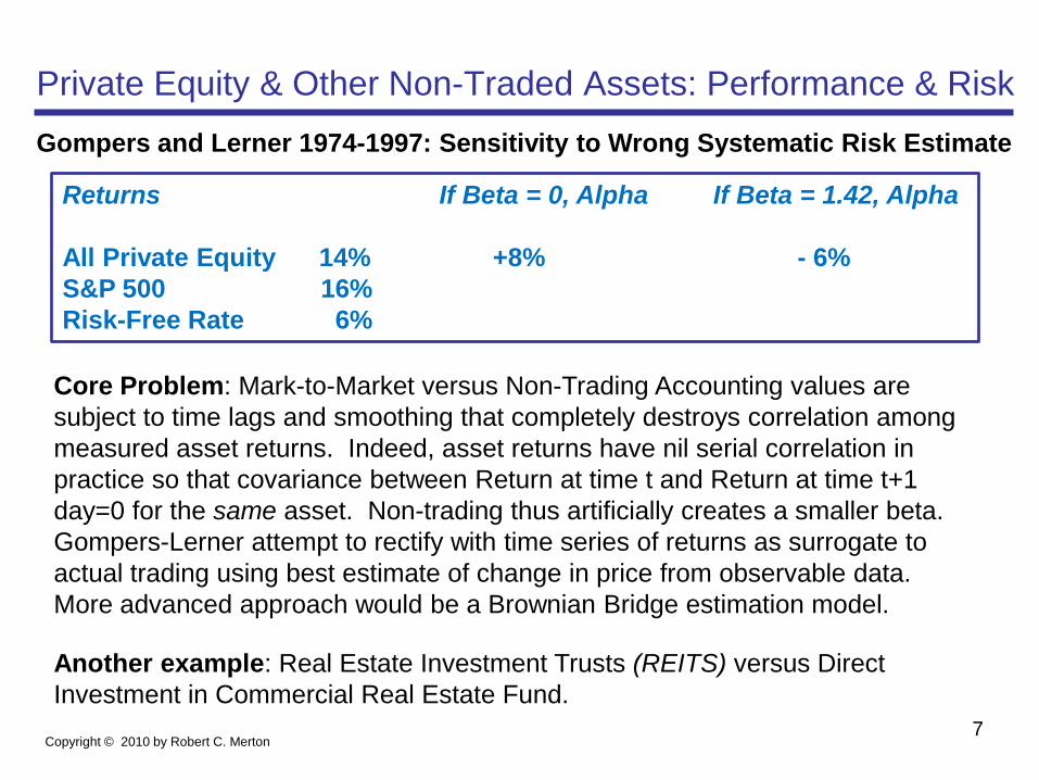
Private Equity & Other Non-Traded Assets: Performance & Risk

Returns If Beta = 0, Alpha If Beta = 1.42, Alpha

All Private Equity 14% +8% - 6%

S&P 500 16%

Risk-Free Rate 6%

Core Problem: Mark-to-Market versus Non-Trading Accounting values are

subject to time lags and smoothing that completely destroys correlation among

measured asset returns. Indeed, asset returns have nil serial correlation in

practice so that covariance between Return at time t and Return at time t+1

day=0 for the same asset. Non-trading thus artificially creates a smaller beta.

Gompers-Lerner attempt to rectify with time series of returns as surrogate to

actual trading using best estimate of change in price from observable data.

More advanced approach would be a Brownian Bridge estimation model.

Another example: Real Estate Investment Trusts (REITS) versus Direct

Investment in Commercial Real Estate Fund.

Gompers and Lerner 1974-1997: Sensitivity to Wrong Systematic Risk Estimate


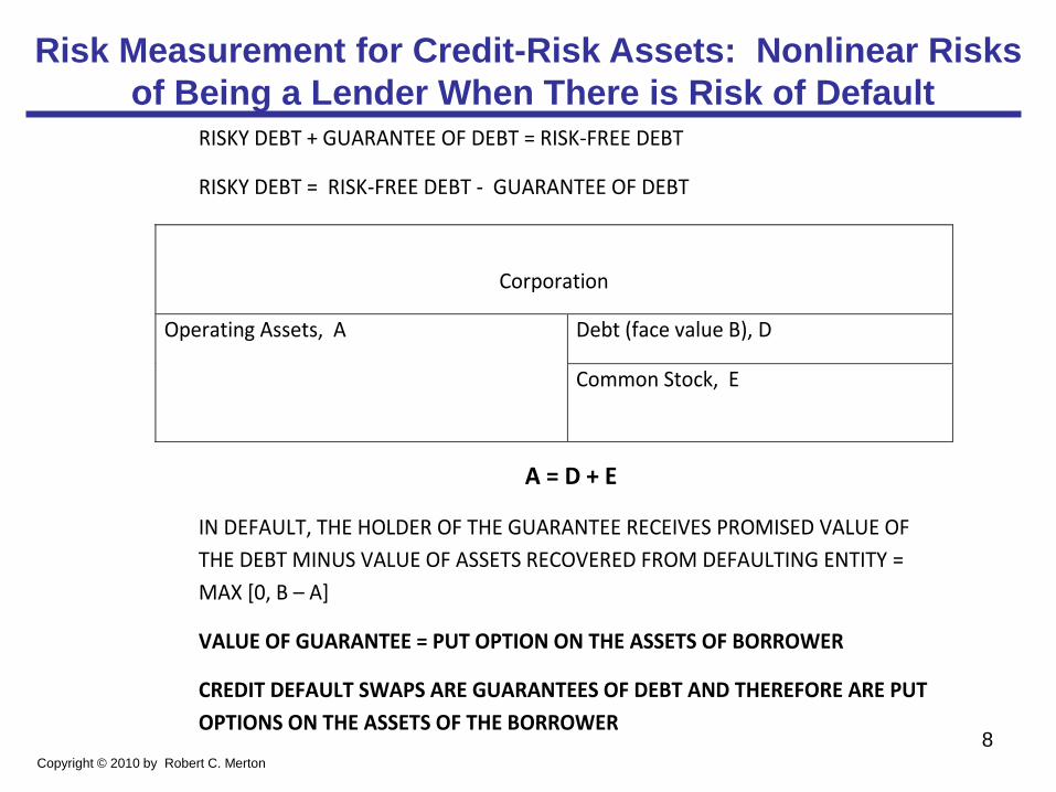
Risk Measurement for Credit-Risk Assets: Nonlinear Risks

of Being a Lender When There is Risk of Default

8 Copyright © 2010 by Robert C. Merton

RISKY DEBT + GUARANTEE OF DEBT = RISK-FREE DEBT

RISKY DEBT = RISK-FREE DEBT - GUARANTEE OF DEBT

A = D + E

IN DEFAULT, THE HOLDER OF THE GUARANTEE RECEIVES PROMISED VALUE OF

THE DEBT MINUS VALUE OF ASSETS RECOVERED FROM DEFAULTING ENTITY =

MAX [0, B – A]

VALUE OF GUARANTEE = PUT OPTION ON THE ASSETS OF BORROWER

CREDIT DEFAULT SWAPS ARE GUARANTEES OF DEBT AND THEREFORE ARE PUT

OPTIONS ON THE ASSETS OF THE BORROWER

Corporation

Operating Assets, A Debt (face value B), D

Common Stock, E

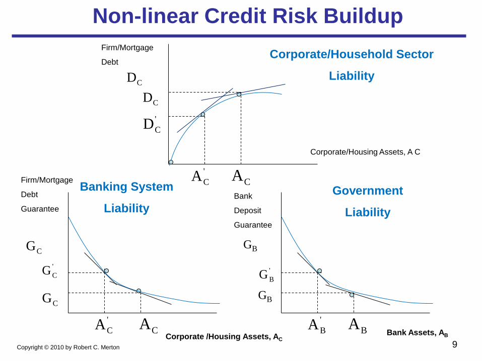
Non-linear Credit Risk Buildup

Firm/Mortgage

Debt

Guarantee

Bank

Deposit

Guarantee

GB

'

BA

'

BG

GB

BA

'

CG

CG

'

CA CA

CG


'

CA CA

'

CD

CD

Firm/Mortgage

Debt

CD

Corporate/Household Sector

Liability

Banking System

Liability

Government

Liability

Corporate/Housing Assets, A C

Bank Assets, AB Corporate /Housing Assets, AC

9

Performance Measurement: Market Timing and

Nonlinear Risk Hedge Funds

For Perfect Market Timing and No Borrowing or Short-Selling

Measuring Return to Market Timing

Call Returnp f m f pR R a b R R c e

Hedge Fund Relative-Value Strategy [risk level change is negatively

correlated with returns]



,

,

p f m f

m f f m

R R Max O R R

R R Max O R R

,p f m f m f pR R a b R R c Max O R R e

Hedge Fund Momentum/Stop-Loss Strategy [risk level change is positively

correlated with returns]

Market Timing [A “free” call or a “free” put]


10

Beyond VAR: Put Option Price for the Portfolio

as a Tail-Risk Indicator

What is the minimum value of our portfolio at the end of time h with probability

1 – p? V (p, h)

What is the amount that the portfolio could lose it or more with probability p at

the end of time h? VaR (p, h) = V (0) – V (p,h)

Put Option Price Reflects Rare-But-Significant Events

• Robust with respect to probability distribution

• Intuitive because the put price is the price of insuring the downside tail

• Reflects a price for insurance versus self-insurance amount of capital

• Jarrow and Van Deventer, GARP Risk Professional, August 2009

Value-at-Risk (VaR): Summary Risk Measure

V(h)

(p, h) V(0) (h)


Integrated Systemic Risk Policy: Refinancing

Ratchet Effect 1996-2006

• Trend #1: rising U.S. home prices

• Trend #2: declining U.S. interest rates

• Trend #3: increasing efficiency of mortgage refinancing

• Each trend taken individually is beneficial or benign

• All three trends superimposed creates unintended

synchronization of homeowner leverage

• Leveraging can be done incrementally, but deleveraging

cannot due to indivisibility of owner-occupied residential

housing

• Result: residential mortgage market is six times more

vulnerable and estimated losses of $1.2 - $1.5 trillion

between June 2006 and December 2008 12


innovation in the asset management industry: risk ... alpha • institutional rigidities:...

Documents