inland lakes sediment trends: sediment analysis results ... · inland lakes sediment trends:...

Inland Lakes Sediment Trends:

Sediment Analysis Results for Two Michigan Lakes

Final Report: 2000-2001

Crystal Lake Littlefield Lake

Project Team:

Sharon S. Yohn1

David T. Long1

John P. Giesy2

Joel D. Fett1

Kurunthachalam Kannan2

1Environmental & Aqueous Geochemical Laboratories Department of Geological Sciences

Michigan State University East Lansing, Michigan 48824-1115

[email protected]

2Aquatic Toxicology Laboratory Department of Zoology

Michigan State University East Lansing, Michigan 48824-1115

[email protected]

Inland Lakes Sediment Trends: Sediment Analysis Results for Two Michigan Lakes 1

Inland Lakes Sediment Trends: Sediment Analysis Results

for Two Michigan Lakes Table of Contents Acknowledgements......................................................................................... 2 Introduction...................................................................................................... 2 Summary ......................................................................................................... 2 Methods........................................................................................................... 3 Results............................................................................................................. 6

210Pb and sedimentation rates..................................................................... 6 Crystal Lake .............................................................................................. 6 Littlefield Lake........................................................................................... 7

Population densities..................................................................................... 9 Organics..................................................................................................... 10 Chemical sediment chronologies.............................................................. 12

Changes in watershed inputs and within lake production.................... 12 Biogeochemical dynamics...................................................................... 13 Anthropogenic inputs.............................................................................. 14

Concentrations .................................................................................... 14 Anthropogenic accumulation rates..................................................... 24 Sources for anthropogenic elements.................................................. 33

Lead.................................................................................................. 34 Copper.............................................................................................. 37 Cadmium .......................................................................................... 40 Zinc ................................................................................................... 40

Porewater................................................................................................... 46 Sampling recommendations ......................................................................... 47 Works Cited................................................................................................... 48


Inland Lakes Sediment Trends: Sediment Analysis Results for Two Michigan Lakes

Acknowledgements This study was made possible by a grant from the Michigan Department of Environmental Quality, and through the assistance of Neal Godby and Bill Taft. The lakes discussed in this report were sampled on the Environmental Protection Agency’s Research Vessel Mudpuppy, with the assistance of its crew. Metals analysis on the inductively coupled plasma mass spectrometer would not have been possible without Dr. Lina Patino, and our thanks to Lydia Scholle for much assistance in the lab and library.

Introduction Contaminated sediments can directly impact bottom-dwelling organisms and represent a continuing source of toxic substances in aquatic environments that may impact wildlife and humans through food or water consumption (Catallo et al., 1995). Therefore, an understanding of the trends of toxic chemical (e.g., polychlorinated biphenyls, Hg) accumulation in the environment is necessary to assess the current state of Michigan’s surface water quality and to identify potential future problems. A common fate of chemicals in a lake is to associate with fine-grained particulate matter and settle to the bottom (Evans and Rigler, 1983). As this deposition occurs over time, sediments in lakes become a chemical tape recorder of the temporal trends of toxic chemicals in the environment as well as of general environmental change over time (von Guten et al., 1997). Sediment trend monitoring is consistent with the framework for statewide surface water quality monitoring outlined in the January 1997 report prepared by the Michigan Department of Environmental Quality entitled, “A Strategic Environmental Quality Monitoring Program for Michigan’s Surface Waters” (Strategy). A key goal of the Strategy is to measure trends in the quality of Michigan’s surface waters, and one activity designed to examine these trends is the collection and analysis of high-quality sediment cores. This report details the activities and findings of the second year of the sediment trend component of the Strategy, and builds upon the results from the five lakes sampled in 1999 (Year 1)(Simpson et al., 2000). The analytical method for mercury analysis is still being refined, and an addendum to this report will be issued that includes all data and information pertinent to mercury.

Summary Sediment cores were collected from two lakes in 2000 to evaluate the spatial and temporal variations in lake sediment quality in Michigan, and as a continuation of the trend monitoring component of the Strategy (Simpson et al., 2000). Sediment cores were collected from one site in each lake, dated with 210Pb and 137Cs, and analyzed for a suite of metals and organic compounds. Analysis for a suite of metals rather than just target anthropogenic metals (e.g., Pb, Cu) allows for interpretations about the sources for different chemicals. Additionally, porewater was collected from each of the two lakes and analyzed for a similar suite of metals. Spatial data (watershed size and shape, and population densities within the watersheds) were collected for the


two lakes sampled, as well as the five lakes sampled previously. Additional data were collected on the history of the production and consumption of several anthropogenic elements. These results were compared to sediment chemical chronologies to determine sources for anthropogenic metals to the environment. Key findings include:

• Because Littlefield Lake has a disturbed 210Pb profile, the sediment core could not be dated, nor sedimentation rates or focusing factors calculated using 210Pb. Therefore, dates for this lake were estimated using the stable lead profile. Littlefield Lake is a carbonate rich lake (Murphy and Wilkinson, 1980), which may have been mined for marl. This could cause significant disturbance in the 210Pb profile.

• The oldest sediment from Crystal Lake is from 1732, and this lake has a relatively deep mixing zone (6 cm).

• Population densities in most watersheds increased over time, with Cass Lake currently (1990) having the highest population densities and Gratiot Lake the lowest.

• Concentrations of total polyaromatic hydrocarbons (PAHs) in Crystal and Littlefield Lakes are higher than all lakes sampled in Year 1, with the exception of Cass Lake.

• Both Crystal and Littlefield Lakes had one sample with most elements having anomalously high (Crystal Lake) or low (Littlefield Lake) concentrations. The causes of these unusual concentrations are unclear.

• Most element accumulation patterns can be characterized as being influenced by watershed inputs, biogeochemical dynamics, or anthropogenic activities.

• Anthropogenic concentration profiles, anthropogenic inventories, population density correlations, and production consumption data were used to infer some of the dominant sources for lead, copper, cadmium and zinc to inland lakes in Michigan.

• Porewater profiles indicate that remobilization of some elements is occurring, but metals are at concentrations below human health action levels.

Methods Sediment cores were collected from Crystal (Montcalm County) and Littlefield (Isabella County) Lakes in 2000 (Fig. 1). Sediment cores were collected from the deepest portion of each lake using a MC-400 Lake/Shelf Multi-corer. Cores were described and examined for color, texture, and signs of zoobenthos and other disturbance. Cores were then extruded and sectioned at 0.5 cm intervals for the top 8 cm, and at 1 cm intervals for the remainder of the core. Sediment cores were collected in a similar fashion from 6 lakes during the summer of 2001 (Cadillac, Crystal [Benzie County], Hubbard, Mullett, Pawpaw and Whitmore Lakes) (Fig. 1). Analysis of these six lakes will be described in the 2001-2002 report.

210Pb was measured on one sub-core from each lake to determine porosity, accumulated dry mass, sedimentation rates, sediment ages and focusing factors (Freshwater Institute in Winnipeg, Manitoba, Canada). Results from Crystal Lake were verified using 137Cs. Sediments were frozen, freeze-dried and digested by nitric acid in a CEM-MDS-81D microwave (Hewitt and Renyolds, 1990). Standard reference material (NIST SRM 8704 Buffalo River Sediment) and procedural blanks were processed to test for accuracy and contamination. The concentrated-acid digests were filtered through an acid-washed, distilled-deionized water (DDW) rinsed 0.40 µm polycarbonate filter. Samples were then analyzed using a Micromass Platform inductively coupled, plasma, mass spectrometer with hexapole technology (ICP-MS-HEX).

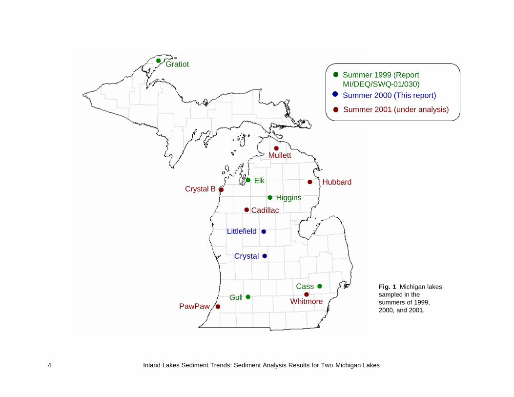
Gratiot

Elk

GullCass

Higgins

Littlefield

Crystal

PawPawWhitmore

Cadillac

Crystal BHubbard

Mullett

Summer 1999 (Report MI/DEQ/SWQ-01/030)Summer 2000 (This report)

Summer 2001 (under analysis)

Fig. 1 Michigan lakes sampled in the summers of 1999, 2000, and 2001.

4 Inland Lakes Sediment Trends: Sediment Analysis Results for Two Michigan Lakes


Sediments were analyzed for a suite of metals and metalloids including Mg, Al, K, Ca, Ti, V, Cr, Mn, Fe, Co, Ni, Cu, Zn, As, Se, Rb, Sr, Mo, Cd, Ba, Pb, and U. High concentrations of calcium in the digested sediment (1500 ppm) made it necessary to add calcium to the standards to match the sample matrix. There were measurable levels of strontium in the calcium standard, making it impossible to quantify strontium levels. However, the trends of strontium are valid, and therefore results are reported in relative concentrations. Another sub-core was sectioned and used for analysis of organic contaminants. There was insufficient material for analysis in the topmost sediments, so the first two sections were combined, and the third and fourth sections were combined. Forty grams of sediment (wet) was homogenized with ≈160 g of anhydrous sodium sulfate and extracted with methylene chloride and hexane (3:1, 400 mL) in a Soxhlet apparatus for 16 h. Sulfur was removed by treating the extracts with activated copper granules. Extracts were then concentrated and passed through a glass column packed with activated Florisil (10 g). The first fraction, eluted with 100mL hexane, contained polychlorinated biphenyls (PCBs), 1,1-dichloro-2,2-bis(p-dichlorodiphenyl)ethylene (p,p’-DDE) and hexachlorobenzene (HCB). The second fraction was eluted with 100 mL of 20% methylene chloride in hexane and contained hexachlorocyclohexane (HCH) isomers (α-, β-, γ-), 1,1-dichloro-2,2-bis(p-chlorophenyl)ethane (p,p’-DDD), dichlorodiphenyltrichloroethane (p,p’-DDT) and chlordane compounds, toxaphene and 16 polycyclic aromatic hydrocarbons (PAHs). The third fraction, eluted with 100 mL of 50% methanol and 50% methylene chloride, contained nonylphenol, octylphenol and other polar compounds. Tetrachloro-m-xylene (TCMX) and PCB 30 were spiked as internal standards to check for recoveries of analytical procedure. Other QA/QC procedures include matrix spikes and analytical blanks. The fourth sub-core was used for the collection of porewater. The sediment core was squeezed 5-6 cm, forcing water through Porex into syringes placed every 1 cm (10 samples) then 2 cm (10 samples) from the top. The collected water was filtered through an acid washed, DDW rinsed 0.40 µm polycarbonate filter and preserved with nitric acid and gold (for mercury analysis). These solutions were analyzed on the ICP-MS-HEX in a similar fashion as the digested sediments. These solutions had significantly lower concentrations of major elements than the digested sediments, eliminating the matrix effects. All spatial data were collected from secondary sources, and were in, or were projected into the Michigan GEOREF coordinate system: oblique Mercator projection, datum NAD83, spheroid GRS 1980. Sources for data included the United States Geological Survey, Michigan Maps and Information (TIGER base data), and Michigan Department of Natural Resource’s spatial data

Porewater collection


library. Census data at the township scale were used for population density calculations. Population data were collected from 1830-1990, but only data after 1870 were used. Watersheds were delineated around each of the seven lakes of interest using Arc/INFO (Boutt et al., 2001). Watersheds generally only encompassed a portion of each township; therefore, to determine population densities within the watershed, it was essential to estimate as accurately as possible where people were living within the township. Thus dasymetric mapping was used to estimate population distribution. Areas that are state owned (surface or fee rights) or areas covered by lakes were considered as non- livable areas. It was assumed that the population was evenly distributed throughout the remaining livable area within each census tract. Anthropogenic accumulation rates of metals were plotted versus population density, and correlation analysis was performed using a best fit, least squares regression line. There are several weaknesses with this type of analysis, and therefore results must be interpreted with care. It was assumed that the population was evenly distributed throughout all areas that were not state owned or water. The preference of people to live near a lake (Stewart, 1994) was not accounted for, causing an underestimation of population densities within watersheds. Additional error was incurred when delineating the watersheds, particularly for lakes with little topography (e.g., Cass Lake). Finally, no attempt was made to account for seasonal increases in population, which may be significant around some of the lakes. All production / consumption data were collected from the Minerals Yearbook, United States Department of the Interior. Analysis included all available data from 1859-1999. Data are for the entire United States unless designated as specific to one state or Canada (Appendix B).

Results 210Pb and sedimentation rates

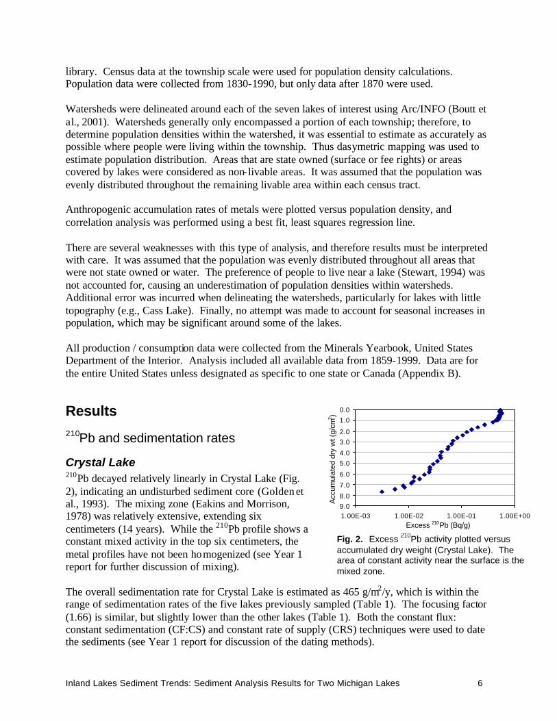
Crystal Lake 210Pb decayed relatively linearly in Crystal Lake (Fig. 2), indicating an undisturbed sediment core (Golden et al., 1993). The mixing zone (Eakins and Morrison, 1978) was relatively extensive, extending six centimeters (14 years). While the 210Pb profile shows a constant mixed activity in the top six centimeters, the metal profiles have not been homogenized (see Year 1 report for further discussion of mixing). The overall sedimentation rate for Crystal Lake is estimated as 465 g/m2/y, which is within the range of sedimentation rates of the five lakes previously sampled (Table 1). The focusing factor (1.66) is similar, but slightly lower than the other lakes (Table 1). Both the constant flux: constant sedimentation (CF:CS) and constant rate of supply (CRS) techniques were used to date the sediments (see Year 1 report for discussion of the dating methods).

0.0

1.0

2.0

3.0

4.0

5.0

6.0

7.0

8.0

9.01.00E-03 1.00E-02 1.00E-01 1.00E+00

Excess 210Pb (Bq/g)

Acc

umul

ated

dry

wt (

g/cm

2 )

Fig. 2. Excess 210Pb activity plotted versus accumulated dry weight (Crystal Lake). The area of constant activity near the surface is the mixed zone.


Table 1. Selected data determined from 210Pb dating, including the oldest section in the core, the focusing factor and average sedimentation rate for lakes sampled in 1999 and 2000. Lake Oldest Section Focusing Factor Ave Sed rate (g/m2/y) Cass 1971 6.00 3480 Elk 1279 2.05 420 Gratiot 1823 2.49 260 Gull 1496 1.78 500 Higgins 1729 2.02 240 Crystal 1732 1.66 465

The 210Pb dating technique was verified using 137Cs. 137Cs is an artificial radionuclide that was produced by atmospheric testing of nuclear weapons in the late 1950s and early 1960s. The peak level of fallout occurred in 1963, and the location of the 137Cs peak in the sediment can be used to verify the accuracy of 210Pb dating (Walling and Qingping, 1992). In Crystal Lake the 137Cs peak occurs in 1982 (CF:CS) or 1977 (CRS). Both dating methods place the cesium peak too recently, but no modifications of the dating methods (e.g., use of the segmented CF:CS (Heyvaert et al., 2000)) significantly altered the date of the cesium peak. Error in the dating may be due to the extensive mixing zone (6 cm, 137Cs peak occurs at 8 cm). Because a more reasonable 137Cs date was obtained from the CRS dating method, these dates will be used throughout the report. The CRS model will tend to propagate errors in 210Pb analysis to the assignment of dates (Heyvaert et al., 2000). This may cause dating errors, particularly for older sediments that are more prone to 210Pb analysis error. However, since this technique seems more appropriate for the younger sediments, it will be used for further analyses. Samples older than 1783 were dated by assuming that the sedimentation rate remained the same as the final sample and should be considered estimations.

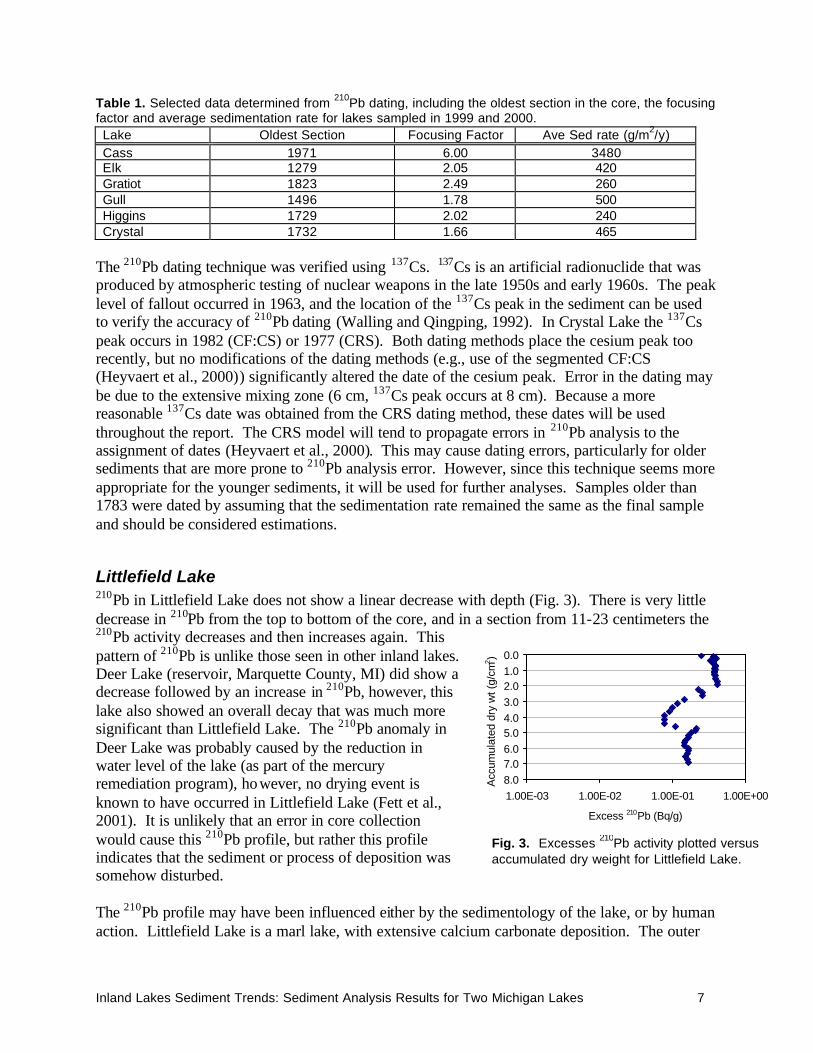
Littlefield Lake 210Pb in Littlefield Lake does not show a linear decrease with depth (Fig. 3). There is very little decrease in 210Pb from the top to bottom of the core, and in a section from 11-23 centimeters the 210Pb activity decreases and then increases again. This pattern of 210Pb is unlike those seen in other inland lakes. Deer Lake (reservoir, Marquette County, MI) did show a decrease followed by an increase in 210Pb, however, this lake also showed an overall decay that was much more significant than Littlefield Lake. The 210Pb anomaly in Deer Lake was probably caused by the reduction in water level of the lake (as part of the mercury remediation program), however, no drying event is known to have occurred in Littlefield Lake (Fett et al., 2001). It is unlikely that an error in core collection would cause this 210Pb profile, but rather this profile indicates that the sediment or process of deposition was somehow disturbed. The 210Pb profile may have been influenced either by the sedimentology of the lake, or by human action. Littlefield Lake is a marl lake, with extensive calcium carbonate deposition. The outer

0.01.02.03.04.05.06.07.08.01.00E-03 1.00E-02 1.00E-01 1.00E+00

Acc

umul

ated

dry

wt (

g/cm

2 )

Excess 210Pb (Bq/g)

Fig. 3. Excesses 210Pb activity plotted versus accumulated dry weight for Littlefield Lake.


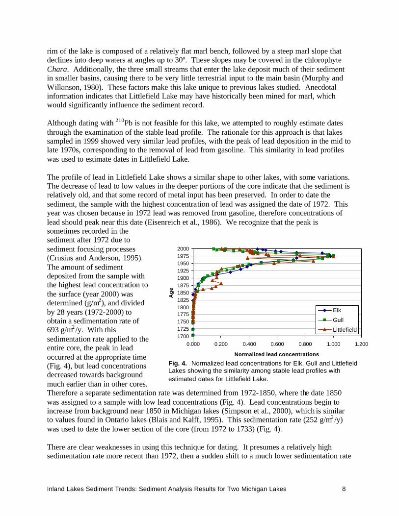
rim of the lake is composed of a relatively flat marl bench, followed by a steep marl slope that declines into deep waters at angles up to 30º. These slopes may be covered in the chlorophyte Chara. Additionally, the three small streams that enter the lake deposit much of their sediment in smaller basins, causing there to be very little terrestrial input to the main basin (Murphy and Wilkinson, 1980). These factors make this lake unique to previous lakes studied. Anecdotal information indicates that Littlefield Lake may have historically been mined for marl, which would significantly influence the sediment record. Although dating with 210Pb is not feasible for this lake, we attempted to roughly estimate dates through the examination of the stable lead profile. The rationale for this approach is that lakes sampled in 1999 showed very similar lead profiles, with the peak of lead deposition in the mid to late 1970s, corresponding to the removal of lead from gasoline. This similarity in lead profiles was used to estimate dates in Littlefield Lake. The profile of lead in Littlefield Lake shows a similar shape to other lakes, with some variations. The decrease of lead to low values in the deeper portions of the core indicate that the sediment is relatively old, and that some record of metal input has been preserved. In order to date the sediment, the sample with the highest concentration of lead was assigned the date of 1972. This year was chosen because in 1972 lead was removed from gasoline, therefore concentrations of lead should peak near this date (Eisenreich et al., 1986). We recognize that the peak is sometimes recorded in the sediment after 1972 due to sediment focusing processes (Crusius and Anderson, 1995). The amount of sediment deposited from the sample with the highest lead concentration to the surface (year 2000) was determined (g/m2), and divided by 28 years (1972-2000) to obtain a sedimentation rate of 693 g/m2 /y. With this sedimentation rate applied to the entire core, the peak in lead occurred at the appropriate time (Fig. 4), but lead concentrations decreased towards background much earlier than in other cores. Therefore a separate sedimentation rate was determined from 1972-1850, where the date 1850 was assigned to a sample with low lead concentrations (Fig. 4). Lead concentrations begin to increase from background near 1850 in Michigan lakes (Simpson et al., 2000), which is similar to values found in Ontario lakes (Blais and Kalff, 1995). This sedimentation rate (252 g/m2 /y) was used to date the lower section of the core (from 1972 to 1733) (Fig. 4). There are clear weaknesses in using this technique for dating. It presumes a relatively high sedimentation rate more recent than 1972, then a sudden shift to a much lower sedimentation rate

1700172517501775180018251850187519001925195019752000

0.000 0.200 0.400 0.600 0.800 1.000 1.200

Normalized lead concentrations

Ag

e

Elk

Gull

Littlefield

Fig. 4. Normalized lead concentrations for Elk, Gull and Littlefield Lakes showing the similarity among stable lead profiles with estimated dates for Littlefield Lake.


immediately after 1972. It is likely that there were several shifts in sedimentation in a disturbed lake such as Littlefield. This dating technique is novel and the dates obtained must be considered a very rough estimation. Because of this, data are plotted versus depth for concentration profiles in Appendix A. Additionally, it is impossible to determine a focusing factor from the 210Pb data, so a focusing factor of two was estimated by averaging all other lakes, with the exception of Cass.

Population densities Watershed sizes vary greatly among the seven lakes sampled (Table 2). Elk Lake has the largest watershed, followed by Higgins Lake. The other lakes have relatively small watersheds compared to these, with Crystal Lake having the smallest. Population densities in 1990 also vary greatly among lakes. The Cass Lake watershed has a significantly higher population density than the other lakes, while the Gratiot Lake watershed has a significantly smaller population density (Table 2).

Table 2. Area of lakes sampled, with sampling depth, watershed area and population densities for 1990.

Lake area Sampling

depth Watershed

area Population

density (1990)

(acres) (ft) (acres) (people/km2) Cass 1280 120 2,251 720.0 Crystal 724 55 1,697 29.7 Elk 7730 193 29,840 35.1 Gratiot 1438 78 6,498 0.6 Gull 2030 110 3,667 54.4 Higgins 9600 136 22,726 57.8 Littlefield 183 70 2,621 11.5

The pattern of population densities over time also varies among lakes (Fig. 5). The Cass Lake watershed population densities have increased significantly since the 1920’s, with greater increases since the 1960’s. Population densities in the Higgins Lake watershed have also increased significantly since 1960, though the values are much lower than Cass Lake. Both Crystal and Littlefield Lakes show relatively little increase in population densities over time in their watersheds, though Crystal Lake has consistently higher population densities than Littlefield Lake. Population densities around Gull

1860

1880

1900

1920

1940

1960

1980

2000

0 10 20 30 40 50 60 70 80

Population density (people/km2)

Dat

e

Gull

Elk

Gratiot

Higgins

Cass / 10

Crystal

Littlefield

Fig. 5. Changes in population density over time for the watersheds of seven lakes in Michigan. Population densities for Cass Lake were divided by 10.

Watershed


Lake began increasing in 1940, but from 1980-90 increased at a much lower rate, indicating a reduction of development around the lake. Population densities around Gratiot Lake were highest in 1860, and decrease to the present, potentially indicating the influence of extensive copper mining. Population densities around Elk Lake peak in the 1900s, decrease, and then increase to the present. The peak in population density around 1900 corresponds to the aluminum peak in the early 1900s, and may show the influence of extensive logging in the area. The relationship between population densities and anthropogenic elements will be examined below.

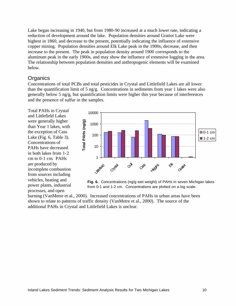
Organics Concentrations of total PCBs and total pesticides in Crystal and Littlefield Lakes are all lower than the quantification limit of 5 ng/g. Concentrations in sediments from year 1 lakes were also generally below 5 ng/g, but quantification limits were higher this year because of interferences and the presence of sulfur in the samples. Total PAHs in Crystal and Littlefield Lakes were generally higher than Year 1 lakes, with the exception of Cass Lake (Fig. 6, Table 3). Concentrations of PAHs have decreased in both lakes from 1-2 cm to 0-1 cm. PAHs are produced by incomplete combustion from sources including vehicles, heating and power plants, industrial processes, and open burning (VanMetre et al., 2000). Increased concentrations of PAHs in urban areas have been shown to relate to patterns of traffic density (VanMetre et al., 2000). The source of the additional PAHs in Crystal and Littlefield Lakes is unclear.

Fig. 6. Concentrations (ng/g wet weight) of PAHs in seven Michigan lakes from 0-1 and 1-2 cm. Concentrations are plotted on a log scale.

1

10

100

1000

10000

Littlefi

eldCrys

tal GullCa

ss

Higgins Elk

Gratiot

To

tal P

AH

s (n

g/g

)

0-1 cm

1-2 cm


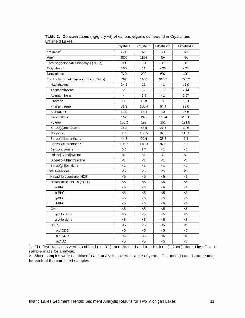
Table 3. Concentrations (ng/g dry wt) of various organic compound in Crystal and Littlefield Lakes. Crystal 1 Crystal 2 Littlefield 1 Littlefield 2

cm depth1 0-1 1-2 0-1 1-2

Age2 2000 1998 NA NA

Total polychlorinated biphenyls (PCBs) < 1 < 1 <1 <1

Octylphenol 100 11 <20 <20

Nonylphenol 720 200 692 409

Total polyaromatic hydrocarbons (PAHs) 767 1008 665.7 776.9

Naphthalene 24.8 21 <1 13.9

Acenaphthylene 5.5 6 1.32 2.14

Acenaphthene 4 3.8 <1 5.07

Fluorene 11 12.9 4 15.4

Phenanthrene 81.9 100.4 64.4 99.6

Anthracene 12.9 14.4 10 13.6

Fluoranthene 197 248 198.4 266.8

Pyrene 156.2 192 152 191.8

Benzo[a]anthracene 26.2 52.5 27.6 39.6

Chrysene 90.5 136.5 87.6 118.2

Benzo[b]fluoranthene 44.8 99.6 33.2 2.5

Benzo[k]fluoranthene 105.7 118.3 87.2 8.2

Benzo[a]pyrene 6.5 2.7 <1 <1

Indeno[123cd]pyrene <1 <1 <1 <1

Dibenzo(a,h)anthracene <1 <1 <1 <1

Benzo[ghi]perylene <1 <1 <1 <1

Total Pesticides <5 <5 <5 <5

Hexachlorobenzene (HCB) <5 <5 <5 <5

Hexachlorohexanes (HCHs) <5 <5 <5 <5

a-BHC <5 <5 <5 <5

b-BHC <5 <5 <5 <5

g-BHC <5 <5 <5 <5

d-BHC <5 <5 <5 <5

CHLs <5 <5 <5 <5

g-chlordane <5 <5 <5 <5

a-chlordane <5 <5 <5 <5

DDTs <5 <5 <5 <5

p,p' DDE <5 <5 <5 <5

p,p' DDD <5 <5 <5 <5

p,p' DDT <5 <5 <5 <5

1. The first two slices were combined (cm 0-1), and the third and fourth slices (1-2 cm), due to insufficient sample mass for analysis. 2. Since samples were combined1 each analysis covers a range of years. The median age is presented for each of the combined samples.


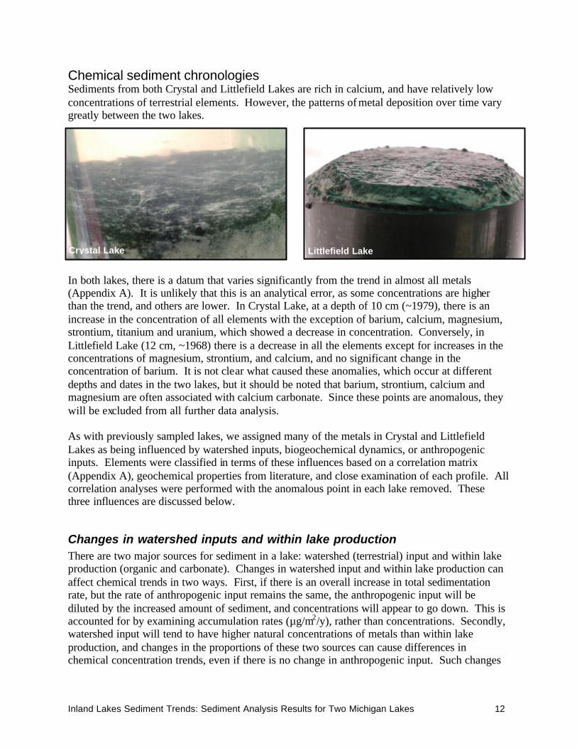
Chemical sediment chronologies Sediments from both Crystal and Littlefield Lakes are rich in calcium, and have relatively low concentrations of terrestrial elements. However, the patterns of metal deposition over time vary greatly between the two lakes.

In both lakes, there is a datum that varies significantly from the trend in almost all metals (Appendix A). It is unlikely that this is an analytical error, as some concentrations are higher than the trend, and others are lower. In Crystal Lake, at a depth of 10 cm (~1979), there is an increase in the concentration of all elements with the exception of barium, calcium, magnesium, strontium, titanium and uranium, which showed a decrease in concentration. Conversely, in Littlefield Lake (12 cm, ~1968) there is a decrease in all the elements except for increases in the concentrations of magnesium, strontium, and calcium, and no significant change in the concentration of barium. It is not clear what caused these anomalies, which occur at different depths and dates in the two lakes, but it should be noted that barium, strontium, calcium and magnesium are often associated with calcium carbonate. Since these points are anomalous, they will be excluded from all further data analysis. As with previously sampled lakes, we assigned many of the metals in Crystal and Littlefield Lakes as being influenced by watershed inputs, biogeochemical dynamics, or anthropogenic inputs. Elements were classified in terms of these influences based on a correlation matrix (Appendix A), geochemical properties from literature, and close examination of each profile. All correlation analyses were performed with the anomalous point in each lake removed. These three influences are discussed below.

Changes in watershed inputs and within lake production There are two major sources for sediment in a lake: watershed (terrestrial) input and within lake production (organic and carbonate). Changes in watershed input and within lake production can affect chemical trends in two ways. First, if there is an overall increase in total sedimentation rate, but the rate of anthropogenic input remains the same, the anthropogenic input will be diluted by the increased amount of sediment, and concentrations will appear to go down. This is accounted for by examining accumulation rates (µg/m2/y), rather than concentrations. Secondly, watershed input will tend to have higher natural concentrations of metals than within lake production, and changes in the proportions of these two sources can cause differences in chemical concentration trends, even if there is no change in anthropogenic input. Such changes

Crystal Lake Littlefield Lake


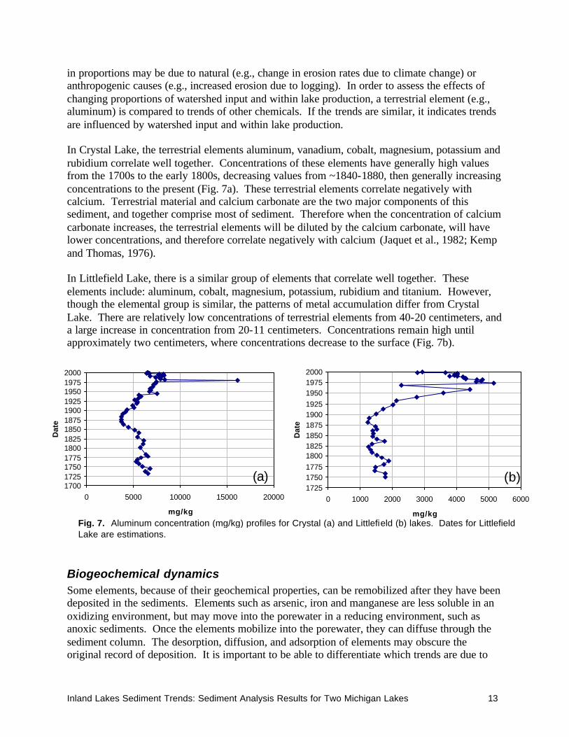
in proportions may be due to natural (e.g., change in erosion rates due to climate change) or anthropogenic causes (e.g., increased erosion due to logging). In order to assess the effects of changing proportions of watershed input and within lake production, a terrestrial element (e.g., aluminum) is compared to trends of other chemicals. If the trends are similar, it indicates trends are influenced by watershed input and within lake production. In Crystal Lake, the terrestrial elements aluminum, vanadium, cobalt, magnesium, potassium and rubidium correlate well together. Concentrations of these elements have generally high values from the 1700s to the early 1800s, decreasing values from ~1840-1880, then generally increasing concentrations to the present (Fig. 7a). These terrestrial elements correlate negatively with calcium. Terrestrial material and calcium carbonate are the two major components of this sediment, and together comprise most of sediment. Therefore when the concentration of calcium carbonate increases, the terrestrial elements will be diluted by the calcium carbonate, will have lower concentrations, and therefore correlate negatively with calcium (Jaquet et al., 1982; Kemp and Thomas, 1976). In Littlefield Lake, there is a similar group of elements that correlate well together. These elements include: aluminum, cobalt, magnesium, potassium, rubidium and titanium. However, though the elemental group is similar, the patterns of metal accumulation differ from Crystal Lake. There are relatively low concentrations of terrestrial elements from 40-20 centimeters, and a large increase in concentration from 20-11 centimeters. Concentrations remain high until approximately two centimeters, where concentrations decrease to the surface (Fig. 7b).

Biogeochemical dynamics Some elements, because of their geochemical properties, can be remobilized after they have been deposited in the sediments. Elements such as arsenic, iron and manganese are less soluble in an oxidizing environment, but may move into the porewater in a reducing environment, such as anoxic sediments. Once the elements mobilize into the porewater, they can diffuse through the sediment column. The desorption, diffusion, and adsorption of elements may obscure the original record of deposition. It is important to be able to differentiate which trends are due to

172517501775180018251850187519001925195019752000

0 1000 2000 3000 4000 5000 6000

mg/kg

Dat

e

1700172517501775180018251850187519001925195019752000

0 5000 10000 15000 20000

mg/kg

Dat

e

Fig. 7. Aluminum concentration (mg/kg) profiles for Crystal (a) and Littlefield (b) lakes. Dates for Littlefield Lake are estimations.

(a) (b)


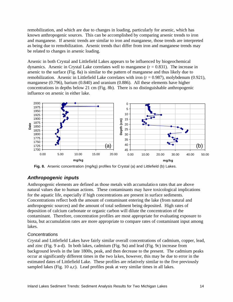
remobilization, and which are due to changes in loading, particularly for arsenic, which has known anthropogenic sources. This can be accomplished by comparing arsenic trends to iron and manganese. If arsenic trends are similar to iron and manganese, those trends are interpreted as being due to remobilization. Arsenic trends tha t differ from iron and manganese trends may be related to changes in arsenic loading. Arsenic in both Crystal and Littlefield Lakes appears to be influenced by biogeochemical dynamics. Arsenic in Crystal Lake correlates well to manganese (r = 0.831). The increase in arsenic to the surface (Fig. 8a) is similar to the pattern of manganese and thus likely due to remobilization. Arsenic in Littlefield Lake correlates with iron (r = 0.987), molybdenum (0.921), manganese (0.796), barium (0.840) and uranium (0.886). All these elements have higher concentrations in depths below 21 cm (Fig. 8b). There is no distinguishable anthropogenic influence on arsenic in either lake.

Anthropogenic inputs Anthropogenic elements are defined as those metals with accumulation rates that are above natural values due to human actions. These contaminants may have toxicological implications for the aquatic life, especially if high concentrations are present in surface sediments. Concentrations reflect both the amount of contaminant entering the lake (from natural and anthropogenic sources) and the amount of total sediment being deposited. High rates of deposition of calcium carbonate or organic carbon will dilute the concentration of the contaminant. Therefore, concentration profiles are most appropriate for evaluating exposure to biota, but accumulation rates are more appropriate to compare rates of contaminant input among lakes.

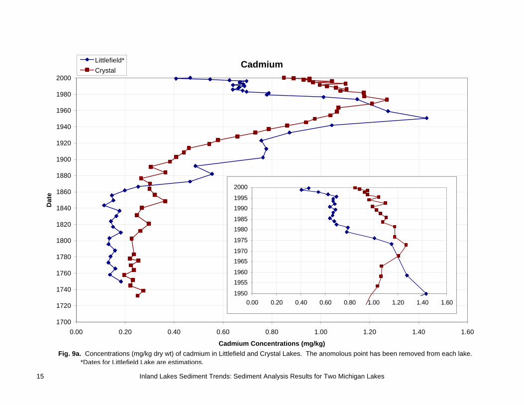
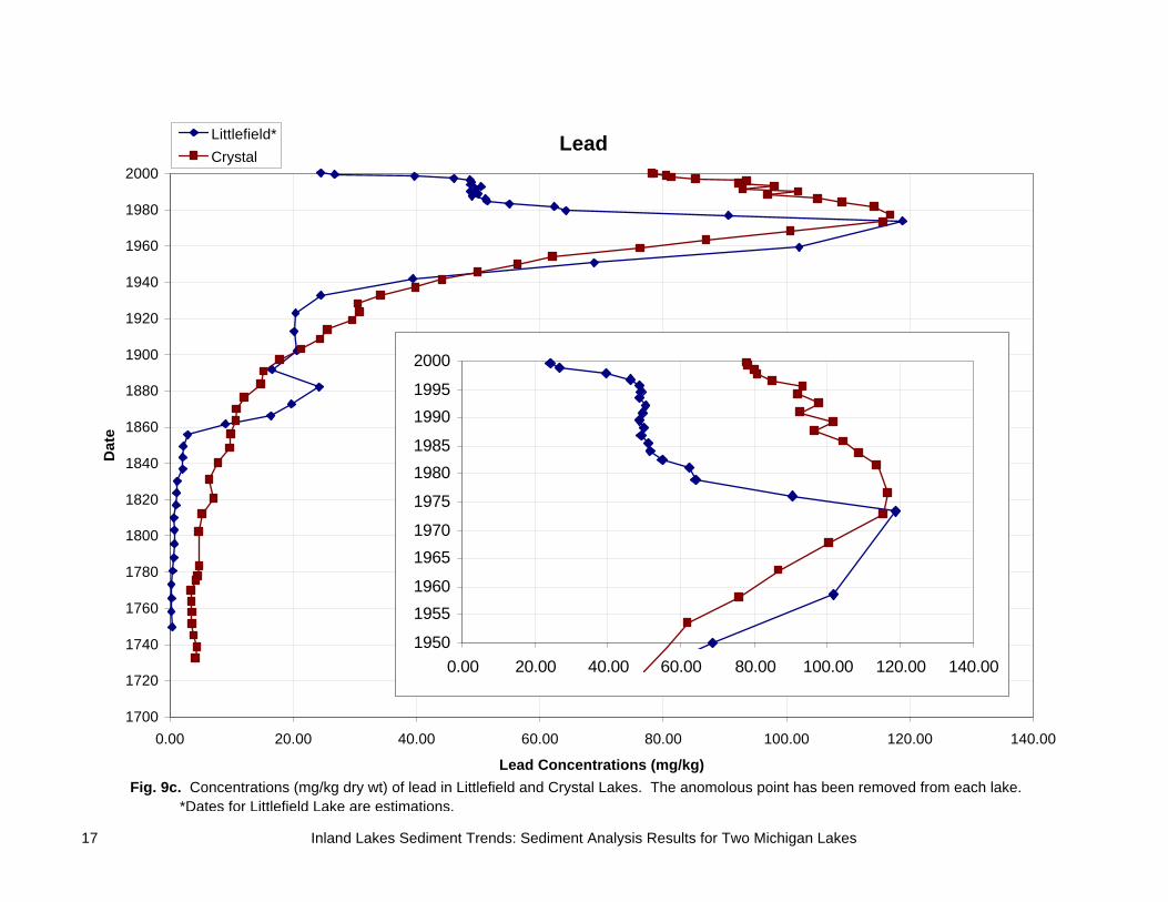
Concentrations Crystal and Littlefield Lakes have fairly similar overall concentrations of cadmium, copper, lead, and zinc (Fig. 9 a-d). In both lakes, cadmium (Fig. 9a) and lead (Fig. 9c) increase from background levels in the late 1800s, peak, and then decrease to the present. The cadmium peaks occur at significantly different times in the two lakes, however, this may be due to error in the estimated dates of Littlefield Lake. These profiles are relatively similar to the five previously sampled lakes (Fig. 10 a,c). Lead profiles peak at very similar times in all lakes.

1700172517501775180018251850187519001925195019752000

0.00 5.00 10.00 15.00 20.00

mg/kg

Dat

e

0

5

10

15

20

25

30

35

40

450.00 10.00 20.00 30.00 40.00 50.00

mg/kg

Dep

th (

cm)

Fig. 8. Arsenic concentration (mg/kg) profiles for Crystal (a) and Littlefield (b) Lakes.

(a) (b)


Cadmium

1700

1720

1740

1760

1780

1800

1820

1840

1860

1880

1900

1920

1940

1960

1980

2000

0.00 0.20 0.40 0.60 0.80 1.00 1.20 1.40 1.60

Cadmium Concentrations (mg/kg)

Dat

e

Littlefield*

Crystal

Fig. 9a. Concentrations (mg/kg dry wt) of cadmium in Littlefield and Crystal Lakes. The anomolous point has been removed from each lake. *Dates for Littlefield Lake are estimations.

1950

1955

1960

1965

1970

1975

1980

1985

1990

1995

2000

0.00 0.20 0.40 0.60 0.80 1.00 1.20 1.40 1.60


Copper

1700

1720

1740

1760

1780

1800

1820

1840

1860

1880

1900

1920

1940

1960

1980

2000

0.00 5.00 10.00 15.00 20.00 25.00

Copper Concentrations (mg/kg)

Dat

e

Littlefield*

Crystal

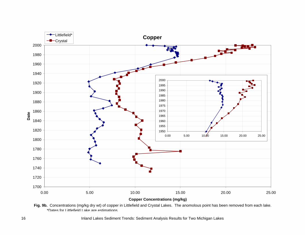
Fig. 9b. Concentrations (mg/kg dry wt) of copper in Littlefield and Crystal Lakes. The anomolous point has been removed from each lake. *Dates for Littlefield Lake are estimations.

1950

1955

1960

1965

1970

1975

1980

1985

1990

1995

2000

0.00 5.00 10.00 15.00 20.00 25.00


Lead

1700

1720

1740

1760

1780

1800

1820

1840

1860

1880

1900

1920

1940

1960

1980

2000

0.00 20.00 40.00 60.00 80.00 100.00 120.00 140.00

Lead Concentrations (mg/kg)

Dat

e

Littlefield*

Crystal

Fig. 9c. Concentrations (mg/kg dry wt) of lead in Littlefield and Crystal Lakes. The anomolous point has been removed from each lake. *Dates for Littlefield Lake are estimations.

1950

1955

1960

1965

1970

1975

1980

1985

1990

1995

2000

0.00 20.00 40.00 60.00 80.00 100.00 120.00 140.00


Zinc

1700

1720

1740

1760

1780

1800

1820

1840

1860

1880

1900

1920

1940

1960

1980

2000

0.00 50.00 100.00 150.00 200.00 250.00

Zinc Concentrations (mg/kg)

Dat

e

Littlefield*

Crystal

Fig. 9d. Concentrations (mg/kg dry wt) of zinc in Littlefield and Crystal Lakes. The anomolous point has been removed from each lake. *Dates for Littlefield Lake are estimations.

1950

1955

1960

1965

1970

1975

1980

1985

1990

1995

2000

0.00 50.00 100.00 150.00 200.00 250.00


Cadmium

1700

1720

1740

1760

1780

1800

1820

1840

1860

1880

1900

1920

1940

1960

1980

2000

0.00 0.50 1.00 1.50 2.00 2.50

Cadmium Concentrations (mg/kg)

Dat

eLittlefield* Crystal CassElk Gratiot GullHiggins

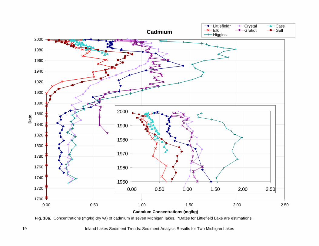
Fig. 10a. Concentrations (mg/kg dry wt) of cadmium in seven Michigan lakes. *Dates for Littlefield Lake are estimations.

1950

1960

1970

1980

1990

2000

0.00 0.50 1.00 1.50 2.00 2.50


Copper

1700

1720

1740

1760

1780

1800

1820

1840

1860

1880

1900

1920

1940

1960

1980

2000

0.00 10.00 20.00 30.00 40.00 50.00 60.00 70.00 80.00

Copper Concentrations (mg/kg)

Dat


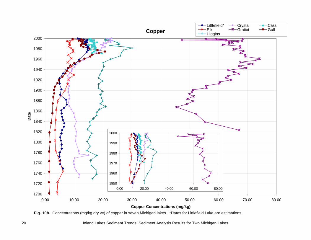
Fig. 10b. Concentrations (mg/kg dry wt) of copper in seven Michigan lakes. *Dates for Littlefield Lake are estimations.

1950

1960

1970

1980

1990

2000

0.00 20.00 40.00 60.00 80.00


Lead

1700

1720

1740

1760

1780

1800

1820

1840

1860

1880

1900

1920

1940

1960

1980

2000

0.00 20.00 40.00 60.00 80.00 100.00 120.00 140.00 160.00 180.00 200.00

Lead Concentrations (mg/kg)

Dat


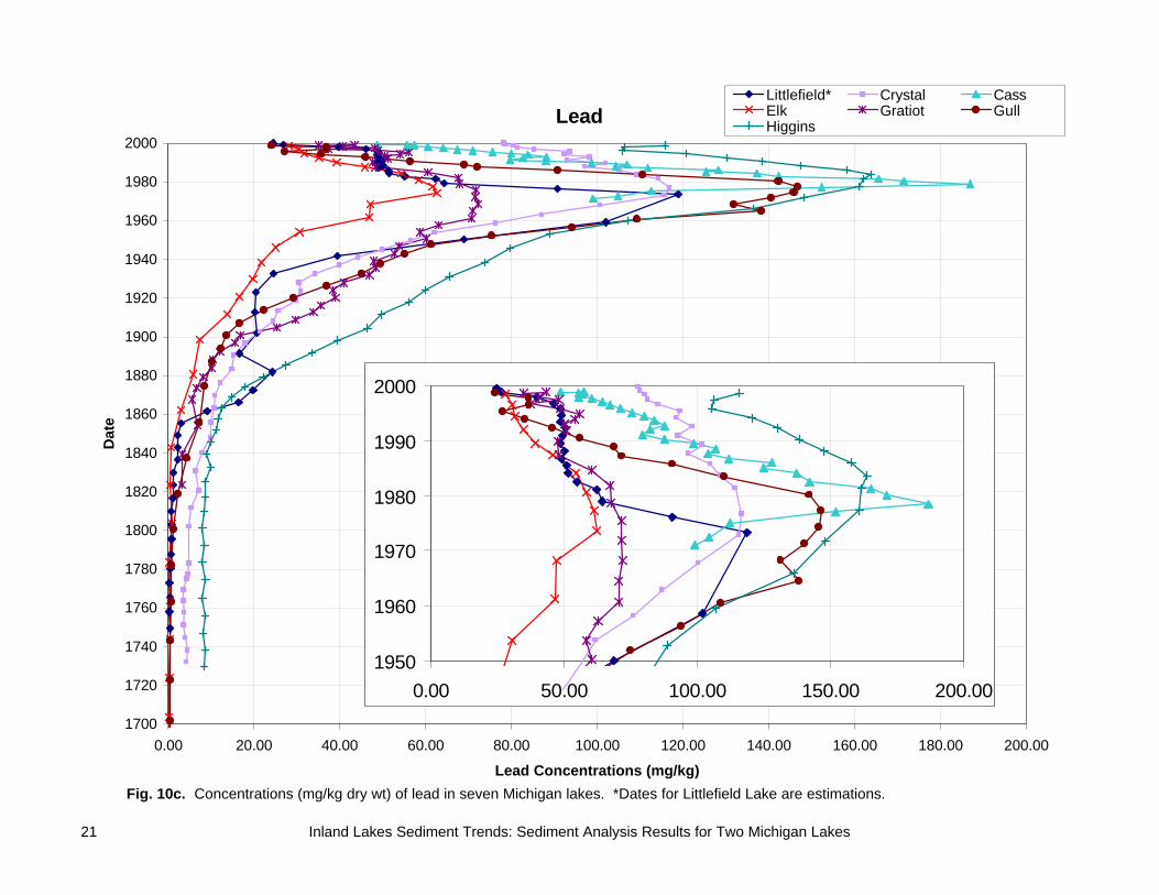
Fig. 10c. Concentrations (mg/kg dry wt) of lead in seven Michigan lakes. *Dates for Littlefield Lake are estimations.

1950

1960

1970

1980

1990

2000

0.00 50.00 100.00 150.00 200.00


Zinc

1700

1720

1740

1760

1780

1800

1820

1840

1860

1880

1900

1920

1940

1960

1980

2000

0.00 50.00 100.00 150.00 200.00 250.00

Zinc Concentrations (mg/kg)

Dat


Fig. 10d. Concentrations (mg/kg dry wt) of zinc in seven Michigan lakes. *Dates for Littlefield Lake are estimations.

1950

1960

1970

1980

1990

2000

0.00 50.00 100.00 150.00 200.00 250.00


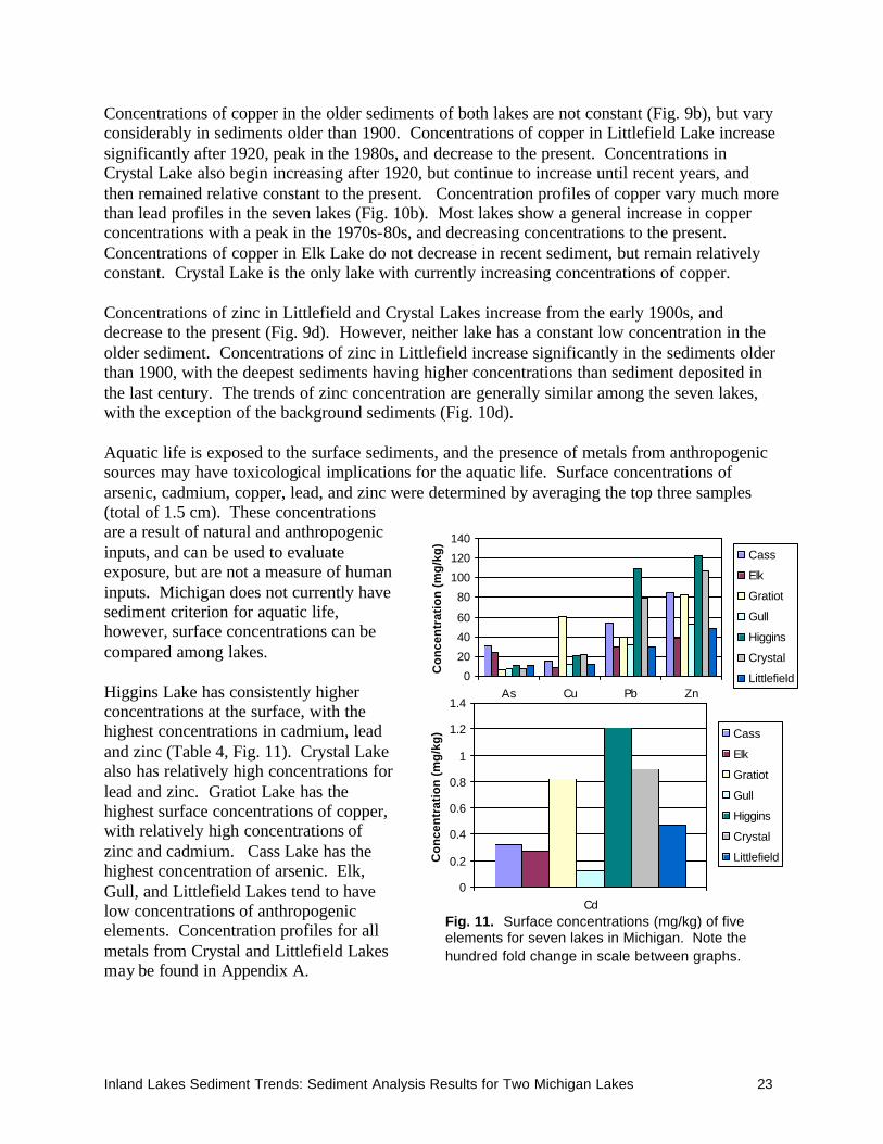
Concentrations of copper in the older sediments of both lakes are not constant (Fig. 9b), but vary considerably in sediments older than 1900. Concentrations of copper in Littlefield Lake increase significantly after 1920, peak in the 1980s, and decrease to the present. Concentrations in Crystal Lake also begin increasing after 1920, but continue to increase until recent years, and then remained relative constant to the present. Concentration profiles of copper vary much more than lead profiles in the seven lakes (Fig. 10b). Most lakes show a general increase in copper concentrations with a peak in the 1970s-80s, and decreasing concentrations to the present. Concentrations of copper in Elk Lake do not decrease in recent sediment, but remain relatively constant. Crystal Lake is the only lake with currently increasing concentrations of copper. Concentrations of zinc in Littlefield and Crystal Lakes increase from the early 1900s, and decrease to the present (Fig. 9d). However, neither lake has a constant low concentration in the older sediment. Concentrations of zinc in Littlefield increase significantly in the sediments older than 1900, with the deepest sediments having higher concentrations than sediment deposited in the last century. The trends of zinc concentration are generally similar among the seven lakes, with the exception of the background sediments (Fig. 10d). Aquatic life is exposed to the surface sediments, and the presence of metals from anthropogenic sources may have toxicological implications for the aquatic life. Surface concentrations of arsenic, cadmium, copper, lead, and zinc were determined by averaging the top three samples (total of 1.5 cm). These concentrations are a result of natural and anthropogenic inputs, and can be used to evaluate exposure, but are not a measure of human inputs. Michigan does not currently have sediment criterion for aquatic life, however, surface concentrations can be compared among lakes. Higgins Lake has consistently higher concentrations at the surface, with the highest concentrations in cadmium, lead and zinc (Table 4, Fig. 11). Crystal Lake also has relatively high concentrations for lead and zinc. Gratiot Lake has the highest surface concentrations of copper, with relatively high concentrations of zinc and cadmium. Cass Lake has the highest concentration of arsenic. Elk, Gull, and Littlefield Lakes tend to have low concentrations of anthropogenic elements. Concentration profiles for all metals from Crystal and Littlefield Lakes may be found in Appendix A.

0

20

40

60

80

100

120

140

As Cu Pb Zn

Co

nce

ntr

atio

n (

mg

/kg

)

Cass

Elk

Gratiot

Gull

Higgins

Crystal

Littlefield

Fig. 11. Surface concentrations (mg/kg) of five elements for seven lakes in Michigan. Note the hundred fold change in scale between graphs.

0

0.2

0.4

0.6

0.8

1

1.2

1.4

Cd

Co

nce

ntr

atio

n (

mg

/kg

) Cass

Elk

Gratiot

Gull

Higgins

Crystal

Littlefield


Table 4. Surface (1.5 cm) concentrations (mg/kg) of five elements for seven lakes in Michigan. mg/kg As Cd Cu Pb Zn

Cass 30.76 0.32 15.35 53.73 85.39 Elk 23.94 0.27 8.77 29.92 38.41 Gratiot 6.64 0.82 60.95 39.53 82.44 Gull 7.64 0.12 11.63 32.42 52.37 Higgins 10.48 1.21 21.05 109.14 122.12 Crystal 7.32 0.9 21.94 78.88 106.48 Littlefield 11.51 0.47 12.16 30.14 49.02

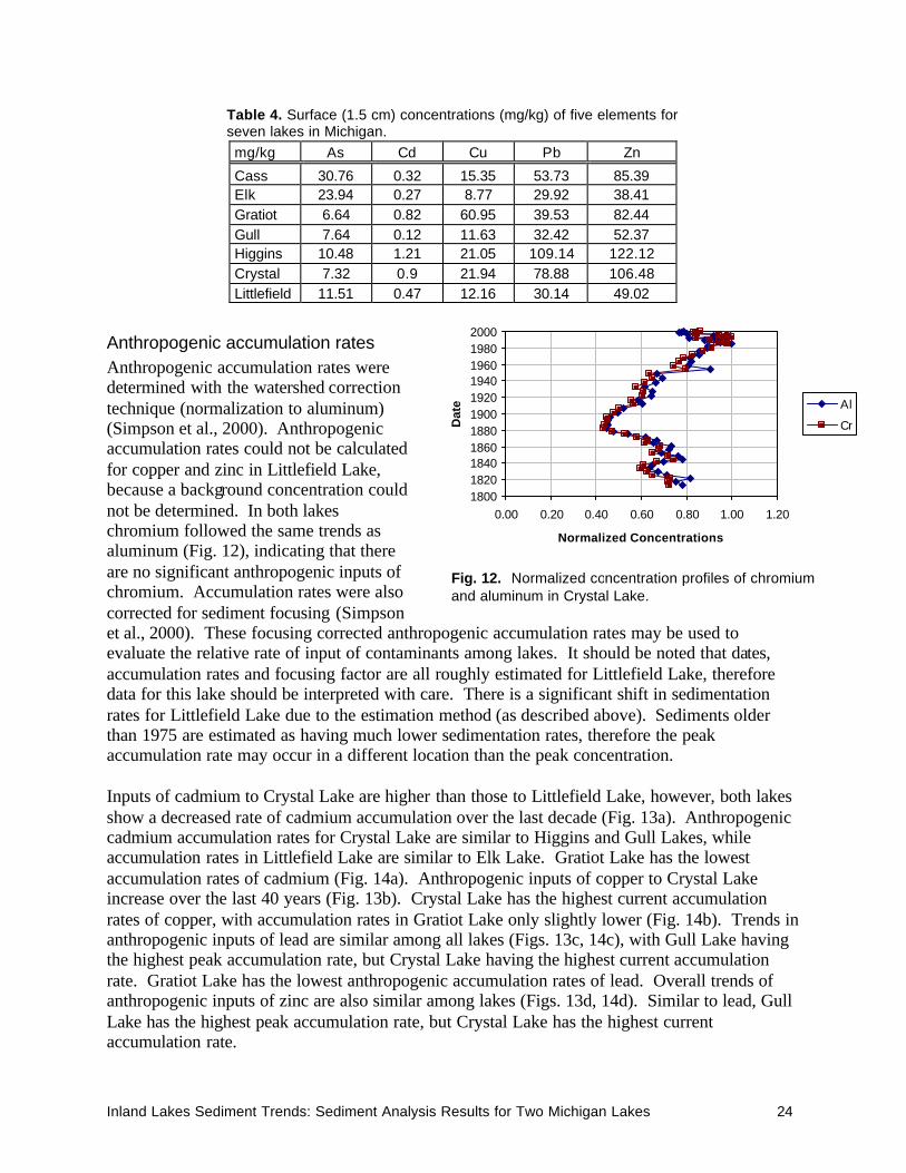
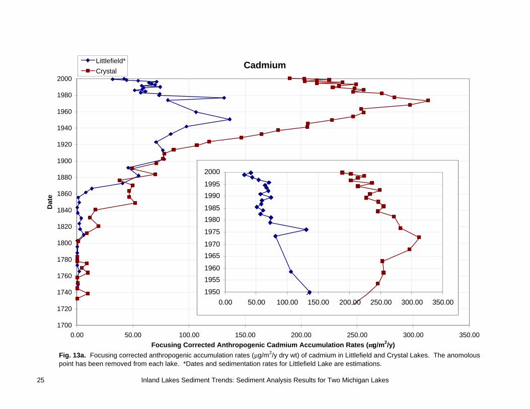
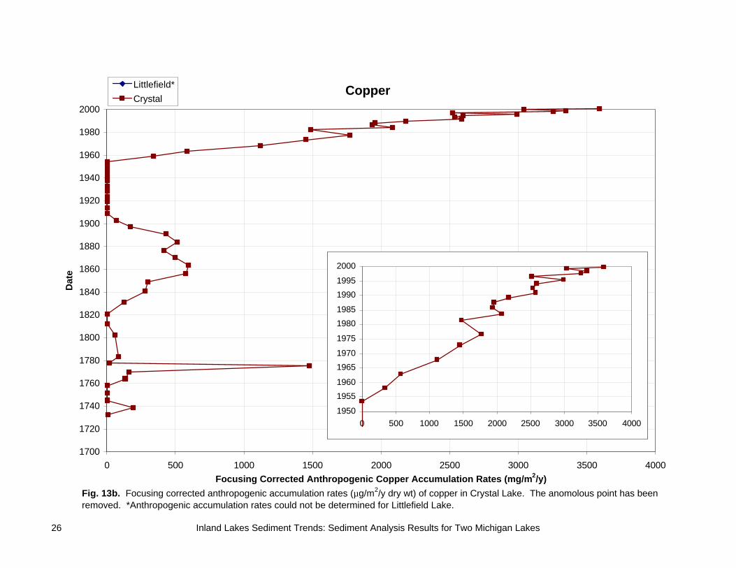
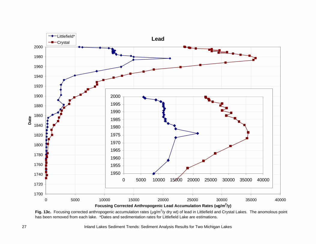
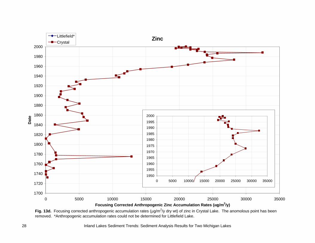
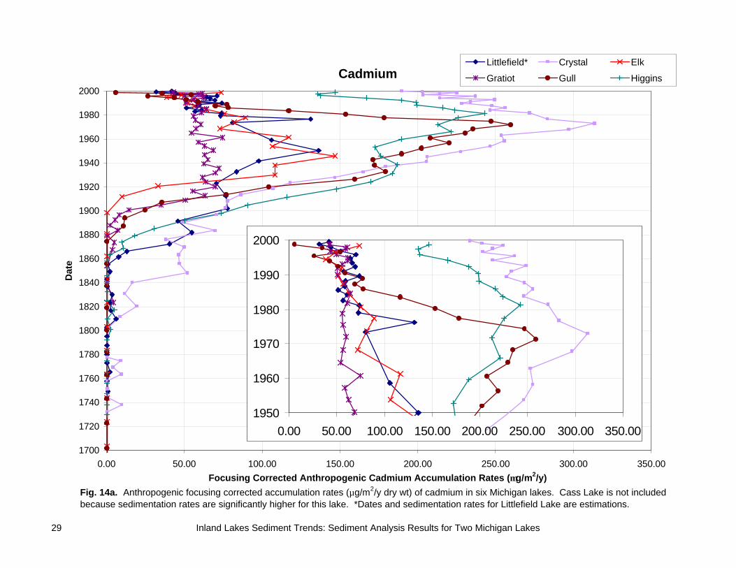
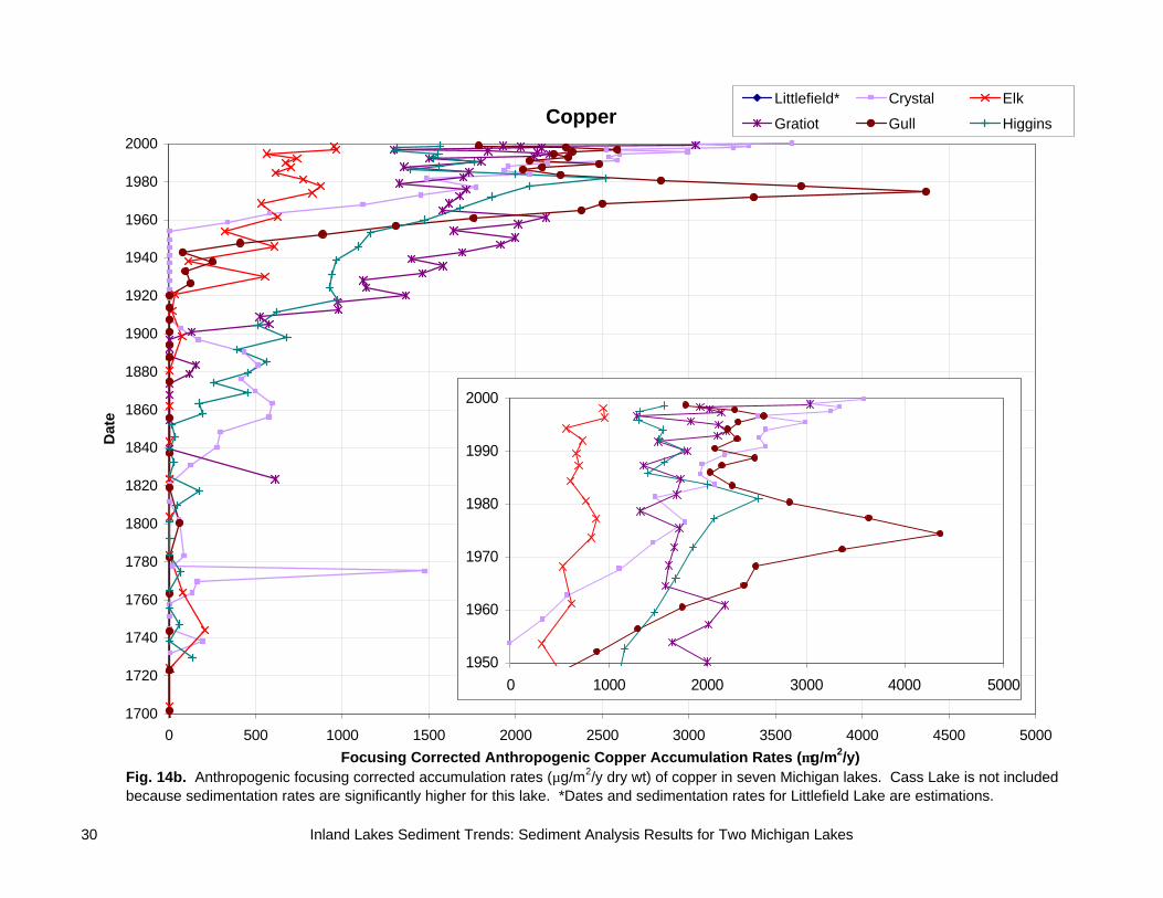
Anthropogenic accumulation rates Anthropogenic accumulation rates were determined with the watershed correction technique (normalization to aluminum) (Simpson et al., 2000). Anthropogenic accumulation rates could not be calculated for copper and zinc in Littlefield Lake, because a background concentration could not be determined. In both lakes chromium followed the same trends as aluminum (Fig. 12), indicating that there are no significant anthropogenic inputs of chromium. Accumulation rates were also corrected for sediment focusing (Simpson et al., 2000). These focusing corrected anthropogenic accumulation rates may be used to evaluate the relative rate of input of contaminants among lakes. It should be noted that dates, accumulation rates and focusing factor are all roughly estimated for Littlefield Lake, therefore data for this lake should be interpreted with care. There is a significant shift in sedimentation rates for Littlefield Lake due to the estimation method (as described above). Sediments older than 1975 are estimated as having much lower sedimentation rates, therefore the peak accumulation rate may occur in a different location than the peak concentration. Inputs of cadmium to Crystal Lake are higher than those to Littlefield Lake, however, both lakes show a decreased rate of cadmium accumulation over the last decade (Fig. 13a). Anthropogenic cadmium accumulation rates for Crystal Lake are similar to Higgins and Gull Lakes, while accumulation rates in Littlefield Lake are similar to Elk Lake. Gratiot Lake has the lowest accumulation rates of cadmium (Fig. 14a). Anthropogenic inputs of copper to Crystal Lake increase over the last 40 years (Fig. 13b). Crystal Lake has the highest current accumulation rates of copper, with accumulation rates in Gratiot Lake only slightly lower (Fig. 14b). Trends in anthropogenic inputs of lead are similar among all lakes (Figs. 13c, 14c), with Gull Lake having the highest peak accumulation rate, but Crystal Lake having the highest current accumulation rate. Gratiot Lake has the lowest anthropogenic accumulation rates of lead. Overall trends of anthropogenic inputs of zinc are also similar among lakes (Figs. 13d, 14d). Similar to lead, Gull Lake has the highest peak accumulation rate, but Crystal Lake has the highest current accumulation rate.

18001820184018601880190019201940196019802000

0.00 0.20 0.40 0.60 0.80 1.00 1.20

Normalized Concentrations

Dat

e Al

Cr

Fig. 12. Normalized concentration profiles of chromium and aluminum in Crystal Lake.


Cadmium

1700

1720

1740

1760

1780

1800

1820

1840

1860

1880

1900

1920

1940

1960

1980

2000

0.00 50.00 100.00 150.00 200.00 250.00 300.00 350.00Focusing Corrected Anthropogenic Cadmium Accumulation Rates (µg/m2/y)

Dat

e

Littlefield*

Crystal

Fig. 13a. Focusing corrected anthropogenic accumulation rates (µg/m2/y dry wt) of cadmium in Littlefield and Crystal Lakes. The anomolous point has been removed from each lake. *Dates and sedimentation rates for Littlefield Lake are estimations.

1950

1955

1960

1965

1970

1975

1980

1985

1990

1995

2000

0.00 50.00 100.00 150.00 200.00 250.00 300.00 350.00


Copper

1700

1720

1740

1760

1780

1800

1820

1840

1860

1880

1900

1920

1940

1960

1980

2000

0 500 1000 1500 2000 2500 3000 3500 4000Focusing Corrected Anthropogenic Copper Accumulation Rates (mg/m2/y)

Dat

e

Littlefield*

Crystal

Fig. 13b. Focusing corrected anthropogenic accumulation rates (µg/m2/y dry wt) of copper in Crystal Lake. The anomolous point has been removed. *Anthropogenic accumulation rates could not be determined for Littlefield Lake.

1950

1955

1960

1965

1970

1975

1980

1985

1990

1995

2000

0 500 1000 1500 2000 2500 3000 3500 4000


Lead

1700

1720

1740

1760

1780

1800

1820

1840

1860

1880

1900

1920

1940

1960

1980

2000

0 5000 10000 15000 20000 25000 30000 35000 40000Focusing Corrected Anthropogenic Lead Accumulation Rates (µg/m2/y)

Dat

e

Littlefield*

Crystal

Fig. 13c. Focusing corrected anthropogenic accumulation rates (µg/m2/y dry wt) of lead in Littlefield and Crystal Lakes. The anomolous point has been removed from each lake. *Dates and sedimentation rates for Littlefield Lake are estimations.

1950

1955

1960

1965

1970

1975

1980

1985

1990

1995

2000

0 5000 10000 15000 20000 25000 30000 35000 40000


Zinc

1700

1720

1740

1760

1780

1800

1820

1840

1860

1880

1900

1920

1940

1960

1980

2000

0 5000 10000 15000 20000 25000 30000 35000Focusing Corrected Anthropogenic Zinc Accumulation Rates (µg/m2/y)

Dat

e

Littlefield*

Crystal

Fig. 13d. Focusing corrected anthropogenic accumulation rates (µg/m2/y dry wt) of zinc in Crystal Lake. The anomolous point has been removed. *Anthropogenic accumulation rates could not be determined for Littlefield Lake.

1950

1955

1960

1965

1970

1975

1980

1985

1990

1995

2000

0 5000 10000 15000 20000 25000 30000 35000


Cadmium

1700

1720

1740

1760

1780

1800

1820

1840

1860

1880

1900

1920

1940

1960

1980

2000

0.00 50.00 100.00 150.00 200.00 250.00 300.00 350.00Focusing Corrected Anthropogenic Cadmium Accumulation Rates (µg/m2/y)

Dat

eLittlefield* Crystal Elk

Gratiot Gull Higgins

Fig. 14a. Anthropogenic focusing corrected accumulation rates (µg/m2/y dry wt) of cadmium in six Michigan lakes. Cass Lake is not included because sedimentation rates are significantly higher for this lake. *Dates and sedimentation rates for Littlefield Lake are estimations.

1950

1960

1970

1980

1990

2000

0.00 50.00 100.00 150.00 200.00 250.00 300.00 350.00


Copper

1700

1720

1740

1760

1780

1800

1820

1840

1860

1880

1900

1920

1940

1960

1980

2000

0 500 1000 1500 2000 2500 3000 3500 4000 4500 5000Focusing Corrected Anthropogenic Copper Accumulation Rates (µg/m2/y)

Dat



Fig. 14b. Anthropogenic focusing corrected accumulation rates (µg/m2/y dry wt) of copper in seven Michigan lakes. Cass Lake is not included because sedimentation rates are significantly higher for this lake. *Dates and sedimentation rates for Littlefield Lake are estimations.

1950

1960

1970

1980

1990

2000

0 1000 2000 3000 4000 5000


Lead

1700

1720

1740

1760

1780

1800

1820

1840

1860

1880

1900

1920

1940

1960

1980

2000

0 5000 10000 15000 20000 25000 30000 35000 40000 45000Focusing Corrected Anthropogenic Lead Accumulation Rates (µg/m2/y)

Dat



Fig. 14c. Anthropogenic focusing corrected accumulation rates (µg/m2/y dry wt) of lead in six Michigan lakes. Cass Lake is not included because sedimentation rates are significantly higher for this lake. *Dates and sedimentation rates for Littlefield Lake are estimations.

1950

1960

1970

1980

1990

2000

0 10000 20000 30000 40000 50000


Zinc

1700

1720

1740

1760

1780

1800

1820

1840

1860

1880

1900

1920

1940

1960

1980

2000

0 5000 10000 15000 20000 25000 30000 35000 40000 45000Focusing Corrected Anthropogenic Zinc Accumulation Rates (µg/m2/y)

Dat



Fig. 14d. Anthropogenic focusing corrected accumulation rates (µg/m2/y dry wt) of zinc in six Michigan lakes. Cass Lake is not included because sedimentation rates are significantly higher for this lake. *Dates and sedimentation rates for Littlefield Lake are estimations.

1950

1960

1970

1980

1990

2000

0 10000 20000 30000 40000 50000


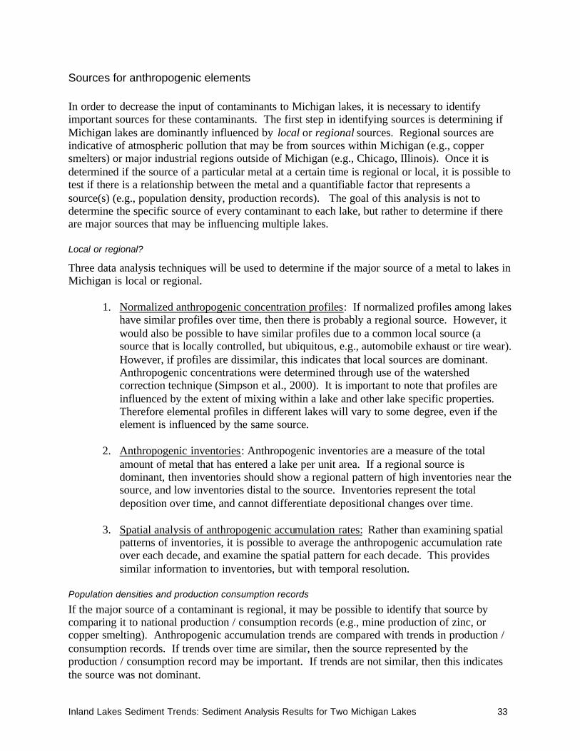
Sources for anthropogenic elements In order to decrease the input of contaminants to Michigan lakes, it is necessary to identify important sources for these contaminants. The first step in identifying sources is determining if Michigan lakes are dominantly influenced by local or regional sources. Regional sources are indicative of atmospheric pollution that may be from sources within Michigan (e.g., copper smelters) or major industrial regions outside of Michigan (e.g., Chicago, Illinois). Once it is determined if the source of a particular metal at a certain time is regional or local, it is possible to test if there is a relationship between the metal and a quantifiable factor that represents a source(s) (e.g., population density, production records). The goal of this analysis is not to determine the specific source of every contaminant to each lake, but rather to determine if there are major sources that may be influencing multiple lakes. Local or regional?

Three data analysis techniques will be used to determine if the major source of a metal to lakes in Michigan is local or regional.

1. Normalized anthropogenic concentration profiles: If normalized profiles among lakes have similar profiles over time, then there is probably a regional source. However, it would also be possible to have similar profiles due to a common local source (a source that is locally controlled, but ubiquitous, e.g., automobile exhaust or tire wear). However, if profiles are dissimilar, this indicates that local sources are dominant. Anthropogenic concentrations were determined through use of the watershed correction technique (Simpson et al., 2000). It is important to note that profiles are influenced by the extent of mixing within a lake and other lake specific properties. Therefore elemental profiles in different lakes will vary to some degree, even if the element is influenced by the same source.

2. Anthropogenic inventories: Anthropogenic inventories are a measure of the total

amount of metal that has entered a lake per unit area. If a regional source is dominant, then inventories should show a regional pattern of high inventories near the source, and low inventories distal to the source. Inventories represent the total deposition over time, and cannot differentiate depositional changes over time.

3. Spatial analysis of anthropogenic accumulation rates: Rather than examining spatial

patterns of inventories, it is possible to average the anthropogenic accumulation rate over each decade, and examine the spatial pattern for each decade. This provides similar information to inventories, but with temporal resolution.

Population densities and production consumption records

If the major source of a contaminant is regional, it may be possible to identify that source by comparing it to national production / consumption records (e.g., mine production of zinc, or copper smelting). Anthropogenic accumulation trends are compared with trends in production / consumption records. If trends over time are similar, then the source represented by the production / consumption record may be important. If trends are not similar, then this indicates the source was not dominant.


Population densities within a lake’s watershed may serve as a proxy for many potential sources, such as sewage, wear from tires, or gasoline emissions. If a relationship at a time interval exists between population densities and anthropogenic accumulation rates of some metal, this would indicate a local common source is dominant. If there is no relationship with population density, it may indicate that there is a unique source to each lake, or that some other factor (e.g., land use in the watershed) that has not yet been evaluated is more appropriate to describe the source. It is important to note that in the following analyses dates, sedimentation rates, and focusing factor for Littlefield Lake were all estimated. Therefore all data for Littlefield Lake must be interpreted with care. Additionally, the anomalous points in Crystal and Littlefield Lakes have been removed for analysis. Lead

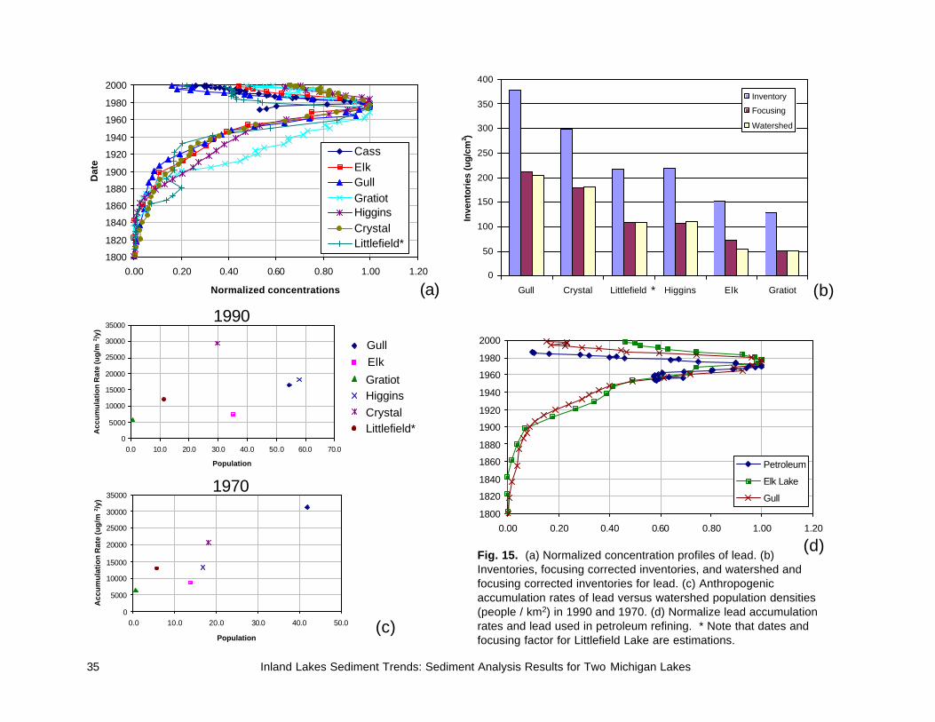
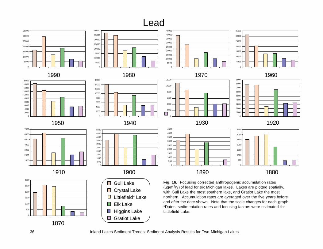
Lead in all of the lakes shows a general increase to the late 1970s, and decreasing concentrations to the present. Normalized anthropogenic concentration profiles are very similar among lakes (Fig. 15a). All lakes have concentrations that increase from background between 1800-1840, increase at a similar rate until the mid to late 1970s and decrease to the present. The rate of decrease differs between lakes. The similarity in these profiles indicates that common local and/or regional sources were dominant from the 1800s to the 1970s, and that local sources or lake processes are dominant in influencing patterns of decreasing lead from the 1970s to the present. Inventories of lead show a definite regional trend, increasing from the north to south in a regular pattern (Fig. 15b). This indicates that a significant portion of the lead that has entered these lakes over time is due to some regional source located to the southwest of Michigan. Spatial analysis of anthropogenic accumulation rates shows a distinct spatial pattern from 1940-1980 (Fig. 16). Littlefield Lake deviates some from the south – north decreasing pattern, but dates, focusing factor and sedimentation rates are all estimated for this lake. Therefore, a regional source appears to be dominant for the deposition of lead to lakes in Michigan for much of the last century, with the pattern changing in the last decade. There is a relationship between population densities and lead accumulation rates in 1970 and 1960 (r2 = 0.812 and 0.843 respectively) (Fig. 15c [note that all population density figures show trends in 1990 and the year with the best correlation between accumulation rates and population densities]). All other dates show little relationship between population densities and lead. This supports the hypothesis that there is some common local source for lead in the 1960s-70s. However, population also correlates with the spatial distribution, with the highest population in the south and decreasing to the north. Because of the similar profiles among the lakes, it seems likely that regional sources are more important than local sources.

1800

1820

1840

1860

1880

1900

1920

1940

1960

1980

2000

0.00 0.20 0.40 0.60 0.80 1.00 1.20

Normalized concentrations

Dat

e

CassElkGullGratiotHigginsCrystalLittlefield*

0

50

100

150

200

250

300

350

400

Gull Crystal Littlefield Higgins Elk Gratiot

Inve

ntor

ies

(ug/

cm2 )

Inventory

Focusing

Watershed

0

5000

10000

15000

20000

25000

30000

35000

0.0 10.0 20.0 30.0 40.0 50.0 60.0 70.0

Population

Acc

um

ula

tio

n R

ate

(ug

/m2 /

y)

0

5000

10000

15000

20000

25000

30000

35000

0.0 10.0 20.0 30.0 40.0 50.0

Population

Acc

um

ula

tio

n R

ate

(ug

/m2 /

y)

1990

1970

1800

1820

1840

1860

1880

1900

1920

1940

1960

1980

2000

0.00 0.20 0.40 0.60 0.80 1.00 1.20

Petroleum

Elk Lake

Gull

(a) (b)

(c)

(d)Fig. 15. (a) Normalized concentration profiles of lead. (b) Inventories, focusing corrected inventories, and watershed and focusing corrected inventories for lead. (c) Anthropogenic accumulation rates of lead versus watershed population densities(people / km2) in 1990 and 1970. (d) Normalize lead accumulation rates and lead used in petroleum refining. * Note that dates and focusing factor for Littlefield Lake are estimations.


Gull

Higgins

Littlefield*Crystal

Gratiot

Elk

*

0

5000

10000

15000

20000

25000

30000

35000

Gull Crystal Littlefield Higgins Elk Gratiot0

5000

10000

15000

20000

25000

30000

35000

40000


0

5000

10000

15000

20000

25000

30000

35000

40000

45000


5000

10000

15000

20000

25000

30000

35000


0

2000

4000

6000

8000

10000

12000

14000

16000

18000

20000


0

2000

4000

6000

8000

10000

12000

14000

16000


2000

4000

6000

8000

10000

12000


1000

2000

3000

4000

5000

6000

7000

8000

9000


0

500

1000

1500

2000

2500

3000

3500

4000

4500

5000


500

1000

1500

2000

2500

3000

3500

4000

4500


500

1000

1500

2000

2500

3000

3500


0

500

1000

1500

2000

2500

3000


Lead

0

1000

2000

3000

4000

5000

6000

7000


1990 1980 1970 1960

1950 19301940 1920

1910 188018901900

1870

Fig. 16. Focusing corrected anthropogenic accumulation rates (µg/m2/y) of lead for six Michigan lakes. Lakes are plotted spatially, with Gull Lake the most southern lake, and Gratiot Lake the mostnorthern. Accumulation rates are averaged over the five years before and after the date shown. Note that the scale changes for each graph. *Dates, sedimentation rates and focusing factors were estimated for Littlefield Lake.


Gull LakeCrystal LakeLittlefield* LakeElk LakeHiggins LakeGratiot Lake


Use of lead in petroleum refining shows a very similar trend to the patterns of lead accumulation within the inland lakes (Fig. 15d). The increase of lead in petroleum refining from the 1950s to the 1970s is very similar to the pattern of increased lead deposition in the lakes, but the decrease in the use of lead in gasoline occurs at a faster rate. This may indicate that there are other sources for lead than use in gasoline, or that lake processes (e.g., mixing) are influencing the profile. It is likely that both of these factors contribute to the differences between the profiles. Overall, inputs of lead to inland lakes in Michigan appear to be influenced significantly by regional atmospheric deposition from Chicago, Illinois and Gary, Indiana industrial areas. However, it appears that local sources have become more important in the last decade (lack of spatial pattern), but this source is not related to population density. Copper

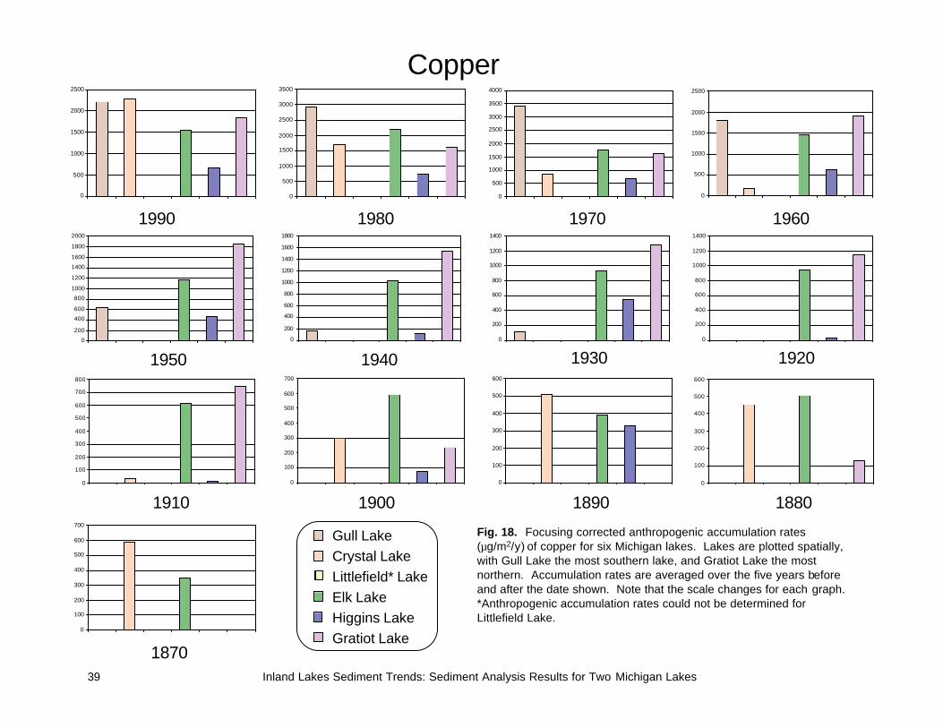
Unlike lead, copper profiles vary greatly among lakes (Fig. 17a). Elk, Gull and Higgins Lakes have high concentrations in the 1970s and generally decrease to the present, though copper in Elk Lake increases in the 1990s. Gratiot Lake has a very broad peak, while Crystal Lake increases to the surface. These differences in profiles indicate that local sources are more important than a regional source. Copper inventories support this conclusion, as there is no apparent regional trend (Fig. 17b). Gratiot Lake has the highest inventory, due to the extensive copper mining that occurs in that region. Accumulation rates also lack a spatial pattern and indicate the importance of local sources (Fig. 18). There is a correlation between population densities and anthropogenic accumulation rates in the 1970s (r2 = 0.960), if Gratiot Lake is removed from the analysis (Fig. 17c). There is little relationship during any other decade. This indicates that there potentially was some important common local source in the 1970s. This relationship only exists for one decade, and therefore must be due to a source that was only dominant for few years, or spurious correlation. Data for additional lakes will clarify the strength of this correlation. There is no close relationship between any production or consumption data (mining, smelter and refinery production, apparent consumption) and the trends within the lakes. There are some large scale similarities in the profiles (general patterns of increasing until the 1970s), but it does not appear that the dominant source of copper is related to these sources. Overall, copper input to inland lakes in Michigan appears to be influenced dominantly by local sources that are unique to each lake. It is possible that in the 1970s there was a common local source such as wastewater. Addition of copper sulfate as a weed deterrent and for simmer’s itch control is a possible local source of copper to lakes in Michigan. It is likely that regional atmospheric deposition contributes some copper to inland lakes, but this does not appear to be the dominant source. The dominant source of copper to Gratiot Lake is probably the extensive copper mining in the region, but these mines and smelters do not appear to have significantly influenced the other lakes studied.

0

500

1000

1500

2000

2500

3000

3500

4000

0.0 10.0 20.0 30.0 40.0 50.0 60.0

Population

Acc

um

ula

tio

n R

ate

(ug

/m2 /y

)

0

500

1000

1500

2000

2500

0.0 10.0 20.0 30.0 40.0 50.0 60.0 70.0

Population

Acc

um

ula

tio

n R

ate

(ug

/m2 /y

)

0

10

20

30

40

50

60

Gull Crystal Higgins Elk Gratiot

Inve

nto

ries

(u

g/c

m2 )

Inventory

Focusing

Watershed

1800

1820

1840

1860

1880

1900

1920

1940

1960

1980

2000

0.00 0.20 0.40 0.60 0.80 1.00 1.20


Dat

e

Cass

Elk

Gull

Gratiot

Higgins

Crystal

1990

1970

(a) (b)

(c)

Fig. 17. (a) Normalized concentration profiles of copper. (b) Inventories, focusing corrected inventories, and watershed and focusing corrected inventories for copper. (c) Anthropogenic accumulation rates of copper versus watershed population densities (people / km2) in 1990 and 1970. * Note that dates for Littlefield Lake are estimations.


Gull

Higgins

Littlefield*Crystal

Gratiot

Elk

Copper

0

500

1000

1500

2000

2500


500

1000

1500

2000

2500

3000

3500


500

1000

1500

2000

2500

3000

3500

4000


0

500

1000

1500

2000

2500


0

200

400

600

800

1000

1200

1400

1600

1800

2000


0

200

400

600

800

1000

1200

1400

1600

1800


200

400

600

800

1000

1200

1400


200

400

600

800

1000

1200

1400


0

100

200

300

400

500

600

700

800


0

100

200

300

400

500

600

700


100

200

300

400

500

600


100

200

300

400

500

600


0

100

200

300

400

500

600

700


Copper

1990 1980 1970 1960

1950 19301940 1920

1910 188018901900

1870

Fig. 18. Focusing corrected anthropogenic accumulation rates (µg/m2/y) of copper for six Michigan lakes. Lakes are plotted spatially, with Gull Lake the most southern lake, and Gratiot Lake the mostnorthern. Accumulation rates are averaged over the five years before and after the date shown. Note that the scale changes for each graph. *Anthropogenic accumulation rates could not be determined for Littlefield Lake.




Cadmium

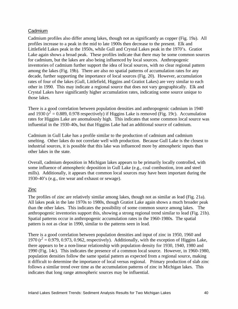
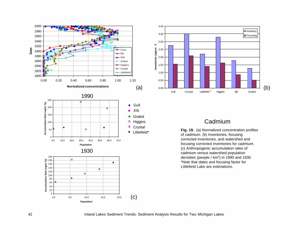
Cadmium profiles also differ among lakes, though not as significantly as copper (Fig. 19a). All profiles increase to a peak in the mid to late 1900s then decrease to the present. Elk and Littlefield Lakes peak in the 1950s, while Gull and Crystal Lakes peak in the 1970’s. Gratiot Lake again shows a broad peak. These profiles indicate that there may be some common sources for cadmium, but the lakes are also being influenced by local sources. Anthropogenic inventories of cadmium further support the idea of local sources, with no clear regional pattern among the lakes (Fig. 19b). There are also no spatial patterns of accumulation rates for any decade, further supporting the importance of local sources (Fig. 20). However, accumulation rates of four of the lakes (Gull, Littlefield, Higgins and Gratiot Lakes) are very similar to each other in 1990. This may indicate a regional source that does not vary geographically. Elk and Crystal Lakes have significantly higher accumulation rates, indicating some source unique to those lakes. There is a good correlation between population densities and anthropogenic cadmium in 1940 and 1930 (r2 = 0.889, 0.978 respectively) if Higgins Lake is removed (Fig. 19c). Accumulation rates for Higgins Lake are anomalously high. This indicates that some common local source was influential in the 1930-40s, but that Higgins Lake had an additional source of cadmium. Cadmium in Gull Lake has a profile similar to the production of cadmium and cadmium smelting. Other lakes do not correlate well with production. Because Gull Lake is the closest to industrial sources, it is possible that this lake was influenced more by atmospheric inputs than other lakes in the state. Overall, cadmium deposition in Michigan lakes appears to be primarily locally controlled, with some influence of atmospheric deposition in Gull Lake (e.g., coal combustion, iron and steel mills). Additionally, it appears that common local sources may have been important during the 1930-40’s (e.g., tire wear and exhaust or sewage). Zinc

The profiles of zinc are relatively similar among lakes, though not as similar as lead (Fig. 21a). All lakes peak in the late 1970s to 1980s, though Gratiot Lake again shows a much broader peak than the other lakes. This indicates the possibility of some common source among lakes. The anthropogenic inventories support this, showing a strong regional trend similar to lead (Fig. 21b). Spatial patterns occur in anthropogenic accumulation rates in the 1960-1980s. The spatial pattern is not as clear in 1990, similar to the patterns seen in lead. There is a good correlation between population densities and input of zinc in 1950, 1960 and 1970 (r2 = 0.979, 0.973, 0.962, respectively). Additionally, with the exception of Higgins Lake, there appears to be a non-linear relationship with population density for 1930, 1940, 1980 and 1990 (Fig. 14c). This indicates the presence of a common local source. However, in 1960-1980, population densities follow the same spatial pattern as expected from a regional source, making it difficult to determine the importance of local versus regional. Primary production of slab zinc follows a similar trend over time as the accumulation patterns of zinc in Michigan lakes. This indicates that long range atmospheric sources may be influential.


Overall, zinc appears to be influenced both by regional atmospheric sources (e.g., zinc production and smelters), as well as common local sources (e.g from the wearing of tires or sewage input), and less by influences by unique local sources.

0

50

100

150

200

250

0.0 10.0 20.0 30.0 40.0 50.0 60.0 70.0

Population

Acc

um

ula

tio

n R

ate

(ug

/m2 /

y)

020

40

60

80100

120

140

160

180200

0.0 5.0 10.0 15.0 20.0

Population

Acc

um

ula

tio

n R

ate

(ug

/m2 /

y)

1800

1820

1840

1860

1880

1900

1920

1940

1960

1980

2000

0.00 0.20 0.40 0.60 0.80 1.00 1.20


Dat

e

1990

1930

(a) (b)

(c)

Fig. 19. (a) Normalized concentration profiles of cadmium. (b) Inventories, focusing corrected inventories, and watershed and focusing corrected inventories for cadmium. (c) Anthropogenic accumulation rates of cadmium versus watershed population densities (people / km2) in 1990 and 1930. *Note that dates and focusing factor for Littlefield Lake are estimations.


Gull

Higgins

Littlefield*Crystal

Gratiot

Elk

0.00

0.50

1.00

1.50

2.00

2.50

3.00

3.50

4.00


Inve

ntor

ies

(ug/

cm2 )

Inventory

Focusing

Cadmium

Cass

Elk

Gull

Gratiot

Higgins

Crystal

Littlefield *

*

0

50

100

150

200

250


50

100

150

200

250

300


50

100

150

200

250

300


50

100

150

200

250

300


0

50

100

150

200

250


20

40

60

80

100

120

140

160

180

200


0

20

40

60

80

100

120

140

160

180

200


20

40

60

80

100

120

140

160

180


0

20

40

60

80

100

120

140


10

20

30

40

50

60

70

80

90


0

10

20

30

40

50

60

70

80


10

20

30

40

50

60


0

5

10

15

20

25

30

35

40

45

50


Cadmium

1990 1980 1970 1960

1950 19301940 1920

1910 188018901900

1870

Fig. 20. Focusing corrected anthropogenic accumulation rates (µg/m2/y) of cadmium for six Michigan lakes. Lakes are plotted spatially, with Gull Lake the most southern lake, and Gratiot Lake the most northern. Accumulation rates are averaged over the five years before and after the date shown. Note that the scale changes for each graph. *Dates, sedimentation rates and focusing factors were estimated for Littlefield Lake.



0

5000

10000

15000

20000

25000

0.0 10.0 20.0 30.0 40.0

Population

Acc

um

ula

tio

n R

ate

(ug

/m2 /y

)

0

5000

10000

15000

20000

25000

30000

0.0 10.0 20.0 30.0 40.0 50.0 60.0 70.0

Population

Acc

um

ula

tio

n R

ate

(ug

/m2 /

y)

0

50

100

150

200

250

300

350

400

450

500

Gull Crystal Higgins Elk Gratiot

Inve

nto

ries

(ug

/cm

2 )

Inventory

Focusing

Watershed

1800

1820

1840

1860

1880

1900

1920

1940

1960

1980

2000

0.00 0.20 0.40 0.60 0.80 1.00 1.20


Dat

e

1990

1950

(a) (b)

(c)

Fig. 21. (a) Normalized concentration profiles of zinc. (b) Inventories, focusing corrected inventories, and watershed and focusing corrected inventories for zinc. Only watershed corrected inventories could be calculated for Crystal Lake. (c) Anthropogenic accumulation rates of zinc versus watershed population densities (people / km2) in 1990 and 1950. *Note that dates for Littlefield Lake are estimations.


Gull

Higgins

Littlefield*Crystal

Gratiot

Elk

Zinc

Cass

Elk

Gull

Gratiot

Higgins

Crystal

Littlefield *

0

5000

10000

15000

20000

25000

30000


5000

10000

15000

20000

25000

30000


0

5000

10000

15000

20000

25000

30000

35000

40000

45000


5000

10000

15000

20000

25000

30000

35000


0

5000

10000

15000

20000

25000


2000

4000

6000

8000

10000

12000

14000

16000


2000

4000

6000

8000

10000

12000

14000


2000

4000

6000

8000

10000

12000


0

1000

2000

3000

4000

5000

6000

7000

8000


1000

2000

3000

4000

5000

6000


0

500

1000

1500

2000

2500

3000

3500

4000

4500


500

1000

1500

2000

2500

3000

3500

4000

4500


0

1000

2000

3000

4000

5000

6000


Zinc

1990 1980 1970 1960

1950 19301940 1920

1910 188018901900

1870

Fig. 22. Focusing corrected anthropogenic accumulation rates (µg/m2/y) of zinc for six Michigan lakes. Lakes are plotted spatially, with Gull Lake the most southern lake, and Gratiot Lake the most northern. Accumulation rates are averaged over the five years before and after the date shown. Note that the scale changes for each graph. *Anthropogenic accumulation rates could not be determined for Littlefield Lake.




Porewater

Sediment chronologies of lakes provide excellent records of changes in chemical accumulation rates, of historical trends and current status, and of newly emerging issues. Surface sediment concentrations also give insight into potential exposure of organisms to chemicals. Often sediment concentrations of chemicals are linked to contaminants in the food chain. An important pathway is release of chemicals from the sediments to water, and then uptake of the water by organisms. Analysis of the porewater within the sediments might provide insights into the degree of this release, processes causing this release, and potential release from deeper sediments that might contain relatively high levels of contaminants.

In this study sediment porewater was analyzed for both Crystal and Littlefield Lakes. These data are some of the first porewater concentration data reported for Michigan’s inland lakes. Profiles of porewater chemical concentrations are shown in Appendix A. The data show that various processes are influencing chemical fate and mobility in the sediments. As more data are accumulated from porewater concentrations and profiles in other lakes, a better understanding of these influences will be obtained. However, some general observations can be made at this time.

In the top few centimeters of sediment, there are major geochemical changes that occur. Organic matter is decomposed, which uses the oxygen in the sediment, and changes the sediment from an oxidizing to a reducing environment. This will change the mobility of many metals, and metals may mobilize from the sediment into the porewater. For example, those metals that are associated with organic matter in the sediment can be released to the porewater as decomposition progresses. Those metals associated with iron and manganese oxy-hydroxides would be released to the porewater when these oxy-hydroxides dissolve because of the reducing conditions. Once in the porewater, metals may move from areas of high concentration to lower concentrations through diffusive flux and/or be readsorbed to other sediments phases. It is clear from the porewater profiles that changes in mobility do occur in the sediments of Crystal and Littlefield Lakes, and that there is mobilization of metals occurring.

One important concern that may be addressed through porewater data is whether or not there is a flux of an element from the sediments to the lake water and the degree to which this is occurring. Ideally this question is addressed by comparing the concentration of an element in the porewater to the concentration in the lake water. If the concentration in the porewater is higher, then diffusive flux will occur. However, even without lake water data, it is possible to draw conclusions for some major elements. If there is a trend in which the porewater concentrations of an element decrease to the surface, this concentration gradient would be evidence for the possible flux of the element from the sediment to the overlying lake water. For example, the porewater profiles for calcium, magnesium and phosphorous all indicate that there is a flux of these elements from the sediment to the lake.

The differences in some of the elemental porewater profiles between the lakes demonstrate the complexity of those processes influencing elemental mobility and thus the difficulty of making generalizations of elemental behavior in the lakes. For example, silica in the porewaters of Littlefield Lake increases with depth and then reaches relatively constant concentrations, while


silica generally increases towards the surface in Crystal Lake, with the last two samples decreasing. Additionally, iron profiles are dissimilar between lakes, with neither lake portraying what might be considered a “typical” iron porewater profile. The typical porewater profile has dissolved iron concentrations that are low near the surface sediments or almost negligible if these sediments are oxidized. Dissolved iron concentrations generally increase to a constant value with depth in the typical profile (Frey and Deevey, 1999; Salomons and Forstner, 1984). Both Littlefield and Crystal Lakes show a subsurface maximum, but then generally decrease with depth.

Further interpretation of porewater profiles will be possible after the examination of more inland lakes. Porewater profiles were collected from six additional lakes in the summer of 2001, and will be discussed in the 2001-2002 final report. However, it is possible to determine from these data that concentrations of anthropogenic elements (e.g., lead, copper), are below action levels (EPA maximum contaminant levels for drinking water) in terms of human health, but could provide possible long-term low level exposure.

Sampling recommendations The first factor that should be considered is the physical constraints of resampling a lake, or the minimum depth that should be deposited before sampling to definitively determine a trend. Only sampling 1.0 cm (two 0.5 cm samples) may not be sufficient to determine a trend. Four samples (2.0 cm) should provide enough data to reliably determine a trend. Therefore the minimum amount of time between sampling will be determined by the sedimentation rate, and the length of time needed to deposit 2.0 cm of new sediment (Table 5).

Table 5. Minimum number of years needed to deposit approximately 2 cm of new sediment for seven inland lakes in Michigan. * Littlefield estimated

Cass Elk Gratiot Gull Higgins Crystal Littlefield* 1 y 10 y 2 y 4 y 6 y 3 y 5 y

Another important consideration is the quality of the core. Littlefield Lake has a disturbed record, and cannot be dated. If this lake were resampled, 210Pb dating could not be used to determine the depth of new deposition. It would be possible to match element profiles to differentiate the depth of new deposition. However, unless there are particular contaminant concerns, resampling this lake is not recommended. An overall monitoring strategy should include:

1. Lakes of concern: lakes with increasing levels of contaminants to the surface, or concentrations of contaminants higher than most other Michigan lakes

2. Background lakes: lakes with low concentrations of contaminants with few point sources in the watershed. These lakes would provide background data on atmospheric deposition and provide a comparison for the lakes of concern. Ideally, these lakes would be spatially dispersed throughout Michigan.

It is not appropriate to make final recommendations on which lakes to monitor until all the preliminary sampling is done, however, some of the lakes may be classified as lakes of concern


or background lakes. Classifying a lake as “of concern” is not an evaluation of the toxicity of the sediments. The lakes that have been most affected by anthropogenic activities are classified as lakes of concern. Cass Lake has clearly been influenced by human activities, and has relatively high concentrations of anthropogenic elements near the surface. Concentrations of anthropogenic elements are also higher than most lakes in Higgins and Crystal Lakes. Of the lakes sampled, these three lakes show the greatest impact from human actions. Elk Lake has consistently low concentrations of contaminants. Gratiot Lake also has low anthropogenic accumulation rates. These two lakes appear to be the “cleanest” of the lakes sampled. After all the preliminary lakes are sampled, it will be possible to determine the lakes with the greatest issues of concern, and other lakes to serve as monitors of contaminants entering lakes with few known point sources.

Works Cited Blais, J. M., and Kalff, J., 1995, The influence of lake morphometry on sediment focusing:

Limnology and Oceanography, v. 40, p. 582-588. Boutt, D. F., Hyndman, D. W., Pijanowski, B. C., and Long, D. T., 2001, Identifying potential

land-use derived solute sources to stream baseflow using groundwater models and GIS: Ground Water, v. 39, p. 24-34.

Catallo, W. J., Schlenker, M., Gambrell, R. P., and Shane, B. S., 1995, Toxic chemicals and trace metals from urban and rural Louisiana lakes: recent historical profiles and toxicological significance: Environmental Science and Technology, v. 29, p. 1439-1446.

Crusius, J., and Anderson, R. F., 1995, Sediment focusing in six small lakes inferred from radionuclide profiles: Journal of Paleolimnology, v. 13, p. 143-155.

Eakins, J. D., and Morrison, R. T., 1978, A new procedure for the determination of lead-210 in lake and marine sediments: International Journal of Applied Radiation and Isotopes, v. 29, p. 531-536.

Eisenreich, S. J., Metzer, N. A., and Urban, N. A., 1986, Response of atmospheric lead to decreased use of lead in gasoline: Environmental Science and Technology, v. 20, p. 171-174.

Evans, R. D., and Rigler, F. H., 1983, A test of lead-210 dating for the measurement of whole lake soft sediment accumulation: Canadian Journal of Fisheries and Aquatic Sciences, v. 40, p. 506-515.

Fett, J. D., Long, D. T., Simpson, S. J., and Patino, L. C., 2001, Temporal Trends in Deer Lake Sediments, Marquette County, Michigan, Michigan Department of Environmental Quality.

Frey, D. G., and Deevey, E. S., 1999, Metals and models: Digenetic modelling in freshwater lacustrine sediments: Journal of Paleolimnology, v. 44, p. 227-251.

Golden, K. A., Wong, C. S., Jeremiason, J. D., Eisenreich, S. J., Sanders, M. G., Hallgren, J., Swackhammer, D. L., Engstrom, D. R., and Long, D. T., 1993, Accumulation and


preliminary inventory of organochlorines in Great Lakes sediments: Water Science Technology, v. 28, p. 19-31.

Hewitt, A. D., and Renyolds, C. M., 1990, Dissolution of metals from soils and sediments with a microwave-nitric acid digestion technique: Atomic Spectroscopy, v. 11, p. 1425-1436.

Heyvaert, A. C., Reuter, J. E., Slotton, D. G., and Goldman, C. R., 2000, Paleolimnological reconstruction of historical atmospheric lead and mercury deposition at Lake Tahoe, California-Nevada: Environmental Science and Technology, v. 34, p. 3588-3597.

Jaquet, J.-M., Davaud, E., Rapin, F., and Vernet, J.-P., 1982, Basic concepts and associated statistical methodology in the geochemical study of lake sediments: Hydrobiologia, v. 91.

Kemp, A. L. W., and Thomas, R. L., 1976, Cultural impacts on the geochemistry of the sediments of Lakes Ontario, Erie and Huron: Water, Air and Soil Pollution, v. 5, p. 469-490.

Murphy, D. H., and Wilkinson, B. H., 1980, Carbonate deposition in a central Michigan marl lake: Sedimentology, v. 27, p. 123-135.

Salomons, W., and Forstner, U., 1984, Metals in the hydrosphere: Berlin, Springer-Verlag, 349 p.

Simpson, S. J., Long, D. T., Geisey, J. P., and Fett, J. D., 2000, Inland lakes sediment trends: sediment analysis results for five Michigan Lakes, MI/DEQ/SWQ-01/030: East Lansing, MI, Department of Environmental Quality, p. 17.

Stewart, S. I., 1994, The seasonal home location decision process: toward a dynamic model: Unpub. Ph.D. thesis, Michigan State University, 156 p.

VanMetre, P. C., Mahler, B. J., and Furlong, E. T., 2000, Urban sprawl leaves its PAH signature: Environmental Science and Technology, v. 34, p. 4064-4070.

von Guten, H. R., Sturm, M., and Moser, R. N., 1997, 200-year record of metals in lake sediments and natural background concentrations: Environmental Science and Technology, v. 31, p. 2193-2197.

Walling, D. E., and Qingping, H., 1992, Interpretation of caesium-137 profiles in lacustrine and other sediments: the role of catchment-derived inputs: Hydrobiologia, v. 235, p. 219-230.

Appendices available upon request

inland lakes sediment trends: sediment analysis results ... · inland lakes sediment trends:...

Documents