infrastructure in the 21st century economy

arm

U.S. Army Corps of Engineers Water Resources Support Center Institute for Water Resources

Infrastructure in the 21st Century Economy An Interim Report - Volume 2 Three Conceptual Papers Exploring the Link Between Public Capital and Productivity

[ DISTRIBUTION STATEMENT II

.Approved tor public leieoMl DumcuooQ Unlimited

OTIC QUALITY INSPECTED 8

Federal Infrastructure Strategy Program

February 1994 IWR Report 94-FIS-8

Federal Infrastructure Strategy Reports

This is the eighth in a series of interim reports which will be published by the U.S. Army Corps of Engineers during the Federal Infrastructure Strategy program, a three-year effort to explore the development of an integrated or multi-agency Federal infrastructure policy. This report introduces and provides an overview of Phase II of a study to assess the impacts of infrastructure on economic growth and productivity.

Other reports in the series thus far include:

Framing the Dialogue: Strategies. Issues and Opportunities (IWR Report 93-FIS-l);

Challenges and Opportunities for Innovation in the Public Works Infrastructure. Volumes 1 and 2. (IWR Reports 93-FIS-2 and 93-FIS-3);

Infrastructure in the 21st Century Economy: A Review of the Issues and Outline of a Study of the Impacts of Federal Infrastructure Investments (IWR Report 93-FIS-4);

Federal Public Works Infrastructure R&D: A New Perspective (IWR Report 93-FIS-5);

The Federal Role in Funding State and Local Infrastructure: Two Reports on Public Works Financing (IWR Report 93-FIS-6);

Infrastructure in the 21st Century Economy: An Interim Report - Volume 1 - The Dimensions of Public Works' Effects on Growth and Industry (IWR Report 93-FIS-7); and

Infrastructure in the 21st Century Economy: An Interim Report - Volume 3 - Data on Federal Capital Stocks and Investment Flows (IWR Report 93-FIS-9);

The program will culminate with a summary report to be published in 1994. The interim documentation contained herein is not intended to foreclose or preclude the program's final conclusions and recommendations. Within this context, comments are welcome on any of these reports.

For further information on the Federal Infrastructure Strategy Program, please contact Robert A. Pietrowsky, Program Manager at :

U.S. Army Corps of Engineers Institute for Water Resources Casey Building 7701 Telegraph Road Alexandria, VA 22315-3868

The Federal Infrastructure Strategy study team includes Cameron E. Gordon, Economic Studies Manager and James F. Thompson, Jr., Engineering Studies Manager. The program is overseen by Dr. Eugene Z. Stakhiv, Chief, Policy and Special Studies Division, and Kyle Schilling, Director of the Institute.

Reports may be ordered by writing (above address) or calling Ms. Arlene Nurthen, IWR Publications, at (703)355-3042.

The Federal Infrastructure Strategy Program

INFRASTRUCTURE IN THE 21ST CENTURY ECONOMY:

AN INTERIM REPORT - VOLUME 2 THREE CONCEPTUAL PAPERS

EXPLORING THE LINK BETWEEN PUBLIC CAPITAL AND PRODUCTIVITY

By

Charles R. Hulten University of Maryland

David Aschauer Bates College

M. Ishaq Nadiri New York University and

National Bureau for Economic Research

Accesion For

NTIS CRA&I DTIC TAB Unannounced Justification

D D

By Distribution /

Availability Codes

Dist

h-l

Avail and/or Special

February 1994 IWR Report 94-FIS-8



TABLE OF CONTENTS

ACKNOWLEDGEMENTS v

PURPOSE OF THIS REPORT vii

ABOUT THE AUTHORS ix

PUBLIC CAPITAL AND ECONOMIC GROWTH: THE MICRO-MACRO LINKAGES - Charles R. Hulten 1

PUBLIC CAPITAL, PRODUCTIVITY, AND MACROECONOMIC PERFORMANCE: A LITERATURE REVIEW - David A. Aschauer 43

INFRASTRUCTURE CAPITAL AND PRODUCTIVITY ANALYSIS: COST- AND PROFIT-FUNCTION APPROACHES - M. Ishaq Nadiri 107

® TABLE OF CONTENTS iii



ACKNOWLEDGEMENTS

This report presents the interim developments in a study of the economic impacts of Federal infrastructure investments in transportation, water resources and supply, and waste management and is one element of a broad administrative directive, undertaken by the U.S. Army Corps of Engineers, and known as the Federal Infrastructure Strategy (FIS).

Special thanks are given to members of the interagency advisory panel which reviewed and analyzed many products and guided the study since its inception. Members in that panel which participated in the interim review meeting came from the Bureau of Reclamation of the U.S. Department of the Interior, the Federal Aviation Administration, Federal Highway Administration and Federal Rail Administration of the Department of Transportation, the Economic Research Service of the U.S. Department of Agriculture, the U.S. Department of the Army, the U.S. Office of Management and Budget, Jack Faucett Associates, the Upjohn Institute of Employment Studies, and the National Science Foundation. Representatives of the U.S. Environmental Protection Agency also provided guidance and useful input. The study's current progress would not have been possible without the vision and contributions of Dr. Charles Hulten of the University of Maryland at College Park, Dr. David Aschauer of Bates College, and Dr. M. Ishaq Nadiri of New York University, and the efforts of staff at Apogee Research, Inc.

Policy guidance for the FIS program is provided by the Office of the Assistant Secretary of the Army (Civil Works) through Dr. Robert N. Stearns, Deputy Assistant Secretary for Project Management, while program execution is overseen by the Corps of Engineers Directorate of Civil Works through Donald Kisicki, Chief, Office of Interagency and International Activities.

The Corps Institute for Water Resources (IWR) has detailed management responsibility for the FIS program under the direction of Dr. Eugene Z. Stakhiv, Chief, Policy and Special Studies Division, and the FIS Study Team which includes Mr. Robert A. Pietrowsky, Program Manager, Mr. Cameron Gordon, Economic Studies Manager, and Mr. James F. Thompson, Jr., Engineering Studies Manager. Mr. Kyle Schilling is Director of the Institute.

This report is presented in three volumes and was prepared under the supervision of Mr. Cameron Gordon, who also wrote the introduction to Volume 1 and prepared the paraphrase proceedings in that volume. Ms. Arlene Nurthen of IWR deserves recognition for her efforts in editing and formatting this report for publication.

® ACKNOWLEDGEMENTS v



PURPOSE OF THIS REPORT

The Federal Infrastructure Strategy (FIS) Program is a collaborative interagency study facilitated by the U.S. Army Corps of Engineers Institute for Water Resources designed to develop and stimulate implementation of an effective policy for managing and maintaining the nation's public works. This report presents developments in one element of that study, namely an effort to delineate and understand the effects of Federal infrastructure investments on the structure and functioning of the U.S. economy and the overall quality of life.

This interim report is a follow-up to a July 1993 publication entitled Infrastructure in the 21st Century Economy: A Review of the Issues and Outline of a Study of the Impacts of Federal Infrastructure Investments (IWR Report 93-FIS-4). That first report described the beginning of the effort in which the Corps presented a "strawman" scope of work to three different panels composed of professional economists and other staff from Federal agencies, Congress and academia, and solicited participation in devising a concrete research plan.

This report describes developments since that initial workplan was articulated and is printed in three volumes. This volume (Volume 2) contains the three technical papers which developed and documented the three research approaches which form this study.

* The first paper, by Dr. Charles Hulten of the University of Maryland at College Park, describes the different theoretical ways in which public capital moves through the economy and suggests that a model known as a Computable General Equilibrium (CGE) model be used to capture and delineate these effects.

* The second paper, by Dr. David Aschauer of Bates College, analyzes how public capital affects the overall economy in the long-run. He describes what is called a dynamic endogenous growth model which will be used to capture these long-term effects and estimate the "optimal" long-run level of public investment as well as how this optimum can be affected by different methods of financing (e.g. deficit versus taxes).

* The third paper, by Dr. Ishaq Nadiri of New York University, addresses the effect of public capital on specific industries and describes an econometric framework, using what are known as cost functions, for estimating infrastructure's impact on productivity within and across different sectors of the economy.

Volume 1 contains an overview of the research effort as it is now being implemented, namely three related research tracks to capture the different dimensions of infrastructure's effects on the economy. The

® PURPOSE OF THIS REPORT vii

introduction to this volume lays out the separate research tracks - one for "telling the story" of how infrastructure investment affects economic structure, one for estimating those impacts numerically, and one for measuring the long-run impact on the macreoconomy - and describes the process which resulted in this research design. Following the introduction is a paraphrase proceedings of the panel meeting, held in October of 1993, in which the research design was analyzed and discussed.

Volume 3 contains the details of a database on public capital collected and developed by Apogee Research, Inc. These data, and other information currently being collected, will feed into all three research tracks, providing for consistency in each of those efforts in the data being analyzed (though one approach may need additional data that another does not). The datasets which have been collected are on investment flows (i.e. annual investments) and capital stocks (collections of annual investments, netting out depreciation) for Federal expenditures in the areas of transportation, water resources and supply, and waste management.

viii PURPOSE OF THIS REPORT ®



ABOUT THE AUTHORS

Dr. Charles Hulten is a Professor of Economics at the University of Maryland at College Park and a Research Associate with the National Bureau of Economic Research, with both places since 1985. Prior to joining the University of Maryland, Dr. Hulten worked for the Urban Institute and Johns Hopkins University, as well as serving as a Visiting Scholar at the American Enterprise Institute. Dr. Hulten has written extensively on regional growth and productivity and the economics of infrastructure investment, among other topics.

Dr. David Aschauer is Elmer W. Campbell Professor of Economics at Bates College. Prior to joining Bates he was a Senior Economist with the Federal Reserve Bank of Chicago and has taught in the graduate schools of the University of Michigan, Northwestern University, and the University of Chicago. He is best known for his work using an aggregate production function to model the economic impacts of public capital investment.

Dr. M. Ishaq Nadiri is currently the Jay Gould Professor of Economics at New York University, where he has been since 1970, and a Research Associate with the National Bureau of Economic Research in New York City. He holds a Ph.D. from the University of California, Berkeley, and has written extensively in the fields of economics of technological change and productivity growth; investment theory and modelling; monetary economics; and applied econometrics.

® ABOUT THE AUTHORS ix



PUBLIC CAPITAL AND ECONOMIC GROWTH: THE MICRO-MACRO LINKAGES

by

Charles R. Hulten, Ph.D. University of Maryland at College Park

October 1993

Report prepared for Apogee Research, Inc. for the U.S. Army Corps of Engineers under Contract DACW72-90-D-0001.

® THE MICRO-MACRO LINKAGES 1

TABLE OF CONTENTS

I. INTRODUCTION 5

II. MODELING THE MACRO-MICRO LINK 7 A. A Simple Economy with Public Capital 7 B. The Production Possibility Frontier and Optimal Public Policy 9 C. Benefit-Cost Analysis 11 D. The Macro Production Function Approach 14 E. Aggregation of Multiple Public Goods 17 F. Dynamic Equilibrium Models 18 G. Public Capital as a Consumer Good 19

III. EXTERNALITIES AND INCREASING RETURNS TO SCALE 21 A. Spillover Externalities 21 B. Increasing Returns to Scale 23

IV. PARTIAL PUBLIC GOODS AND CONGESTION 27 A. The Theory of Public "Clubs" 27 B. Departures from Optimal Policy 27 C. Increasing Returns and Build In Advance of Need 30

V. NETWORK CAPITAL AND SPATIAL EQUILIBRIUM 31 A. Network Issues 31 B. A Closer Look at Output Effects 33 C. Benefit-cost Analysis and the Macro Approach 34

VI. CONCLUSION 37

REFERENCES 39

LIST OF FIGURES

Figure II.1 12 Figure II.2 12 Figure II.3 13 Figure II.4 13 Figure II.5 16 Figure IV.l 28 Figure IV.2 29 Figure V 32


LIST OF TABLES

Table III

4 THE MICRO-MACRO LINKAGES (R)

I. INTRODUCTION

The Office of Management and Budget has "recommended" benefit-cost analysis as the basic tool to use in evaluating government programs and projects (OMB Circular No. A-94). Despite this endorsement, benefit-cost analysis is not always employed at all levels of government, and when it is used, it is sometimes ignored (Goodstein (1993)). This gap between the OMB mandate and actual practice has many causes: the great difficulty in valuing some costs and benefits (e.g., the value of saving a human life), bureaucratic inertia, and political objectives ("demonstration" projects). But there is also an underlying belief that benefit-cost analysis does not always lead to the right result, particularly when very large, capital-intensive programs like the Interstate Highway System are considered. Many of the benefits of large programs are thought to be indirect and thus hard to pin down, and therefore very hard to measure accurately. Thus, many large projects may be rejected by the benefit-cost approach when the true benefits (direct and indirect) justify acceptance of the project.

The emergence of the macro "production function" approach to assessing the benefits of public investment seems to confirm this criticism. The strong correlation between aggregate output and various aggregate measures of public capital suggests that the total effect of public capital on output growth is far stronger than indicated by benefit-cost analysis. By implication, the indirect effects of public investments are very large, and benefit-cost procedures need to be amended or supplemented to account for these important effects.1

Benefit-cost supporters, however, point to a host of econometric problems with the macro production-function approach, and to studies that suggest that the true macro impact of public investment is much smaller than reported in some of the early macro studies. Moreover, many observers have asked the following questions: if there really are significant indirect effects that are missed by benefit-cost analysis, where does one go to find them? Where does one look to see them in action? Or are they discernible only as statistical constructions obtained from an abstract analysis?

These are important issues. For, if those macro production function results that find huge rates of return to public investment are correct, then conventional benefit-cost analysis may miss more than it measures. In this case, reliance on benefit-cost procedures commits the public sector to a systematic under-investment in public capital, and raises the following question: why carry out expensive and time consuming project analysis when it leads to the wrong result? On the other hand, if it is the macro analysis that is flawed, to jettison benefit-cost analysis is to eliminate an important tool of effective government and commit the nation to wasteful building programs at a time when government budgets are greatly constrained.

The over-arching goal of the U.S. Army Corps of Engineers' project on "Assessing the

1 For stylistic reasons, we will use the terms "public capital" and "infrastructure" interchangeably. Although there is a large overlap between the two, they are actually quite different. A significant fraction of the nation's infrastructure is located in the regulated utility sector and owned by private investors, while much of the stock of public capital does not fit the traditional definition of "infrastructure" as social overhead capital. However, given the focus of this paper, we will use the terms to signify those types of capital for which a public benefit-cost analysis might be relevant.

(Q\ THE MICRO-MACRO LINKAGES 5

Economic Effects of Planned Federal Infrastructure Investments" is to sort out these issues. Three general goals are set out in the Scope of Work on this project, and they are to: (1) develop and compare the macro production/cost function method of estimating total rates of return on federally- supported capital projects with the corresponding benefit-cost method; (2) develop simulations of the actual impacts of those investments; and (3) compare the forecasts of the two methods with the simulations of the actual effects.

This report takes up the benefit-cost aspect of goal (1) in the Scope of Work, and describes the idealized benefit-cost analysis in the context of the underlying economic model envisioned in (2). Some comments on the macro production are offered at the same time. Goal (2) is also addressed by considering various aspects of the underlying microeconomic structure that might give rise to a divergence between benefit-cost analysis and the macro production approach. The aspects considered in this paper include an analysis of some of the difficulties that arise when: (a) trying to link (aggregate) micro production functions to a macro production function when the micro technologies are not identical and products and inputs are heterogeneous; (b) when there are spillover externalities at the micro level among producers; (c) when there are internal and external economies of scale; (d) when there is jointness of use in public facilities (i.e., public capital as a congestible public good); (e) when there are complementarities and substitution in spatial networks of interlocking investments.

A valid treatment of the macro-micro link must consider each of the five problem areas set out above, because any of the five can cause the micro and macro analyses of public capital to give divergent results, and each does so in a different way. For example, the macro production-function analysis will give different results from the benefit-cost approach if there are external scale economies among micro units of production. In this case, the macro estimates are likely to be the more valid, and the required "fix" for benefit-cost analysis will require some macro estimation. On the other hand, the problems of partial public goods and congestion are likely to be more accurately reflected in micro analysis. Finally, if network externalities are important, then both the conventional macro production model and benefit-cost analysis are likely to give biased results relative to the true impact of public capital.

Each area has its own literature, which is reviewed in the following sections. Section II develops a model of the micro production structure of a stylized two-sector economy, and reviews aggregation theory in the context of this structure (issue (a)). We then turn to issues (b) and (c), and review the literature on the "new growth theory," which has direct relevance for the issue of the micro-macro link. Section IV considers the problems posed by partial public goods and congestion (d), while Section V deals with the issue of network externalities (e). The various problems with implementing benefit-cost analysis are not reviewed, since they have been treated extensively in other papers and reports (for example, Corps of Engineers (1991) and Lewis (1991)).

The objective of this paper is, in fact, more than a review of relevant literatures under Goal (1) of the Corps of Engineers Scope of Work. The literature survey in each section is intended to be read in the context of Goal (2) as an attempt to lay the groundwork for a simulation model of the economy that is appropriate for assessing the alternative approaches to program analysis. One result of focusing on Goal (2) is that the material presented in the following sections is often of a technical nature. An effort has been made to minimize the use of mathematical notation, but the essential framework is intentionally analytical in its nature.

6 THE MICRO-MACRO LINKAGES ®

II. MODELING THE MACRO-MICRO LINK

A. A Simple Economy with Public Capital

We start by modeling the productivity of public capital in an economy with two industries, one of which uses public capital and one which does not. The first is composed of M firms, each producing a homogeneous output, Yj, using the technology ^'(L^K^G) that exhibits constant returns to scale in labor, L„ privately operated plant and equipment, Ki; and publicly provided capital, G. The total amount of labor and capital used in Industry Y is Ly = E L; and KY = E Ki; respectively, and total industry output is Y = E Yj. Public capital is treated as a pure public good, so each firm gets the same amount, G. These assumptions are summarized in the top panel of Table ILL

Production in the X sector takes places in N firms, each of which has a constant-returns-to-scale production function ^'(L^Kj) that uses labor and private capital, but no public capital. As shown in the second panel of the Table, the total amount of labor and capital used in Industry X is L* = E L;

and Kx = E K;, respectively, and total output is X = E X;.

Industries X and Y are both assumed to be perfectly competitive, which is to say, the firms in both industries maximize profits taking the prevailing output and input prices as given. Since production takes place under constant returns, the value of output is equal to the cost of labor and capital.

Thus, for a firm in Industry X,

(II. 1) PXX; = P^ + PKR,,

where PL is labor's wage and PK is the user cost (or gross return to capital). In Industry Y,

(II.2) PYY = PLL, + PKK,

We assume here that the public input is provided to firms in Industry Y free of charge, and that it raises the marginal product of labor and capital in Industry Y.

Note that the factor prices PL and PK are assumed to be the same for all firms in both industries. By the assumption of perfect competition, relative prices are equal to marginal products, implying

AY P AY P (II. 3) —l=fjiZZi=lÄ

AL. Py'A£(. PY

and

01.4) AX, P^ A^ Px

AL-px'AK~Px

(QS THE MICRO-MACRO LINKAGES 7

TABLE II.l

INDUSTRY Y:

Production Functions

Total Industry Labor Input:

Total Industry Capital Input:

Total Public Input:

Total Industry Output:

INDUSTRY X:

Production Functions

Total Industry Labor Input:

Total Industry Capital Input:

Total Industry Output:

GOVERNMENT:

Production Function:

AGGREGATE ECONOMY:

Production Possibility Frontier:

Real GDP:

Total Labor Input:

Total Capital Input:

M firms

N firms

8 THE MICRO-MACRO LINKAGES (Ä)

Yt =.V(LpKi,G) i = 1.....M

M

LY = E Z, i

M

KY = E K, l

G. = G2 = ■■ = Gu = G

M

Y = E 7.

X. = 4%,K) i = l,...,N

Lx = E L,

Kx = E K,

X = E X

G = 0 (Z^/O

F(Y,X,L,K,) = 0

Fy7 + P^ = PLL + P^

L = LY + Lx + Lc

K =KY + KX + KG

These conditions imply an optimal allocation of labor and capital among the firms of industries X and Y, for a given government policy about the quantity of G to produce.

The stock of public capital is produced by the government sector using the constant returns to scale production function G = ß(LG,KG). The government decides on the quantity of G it wants to provide, and then enters the factor markets to hire the LQ and KG needed to produce this amount. To do this, it must raise PLLG + PKKG dollars in tax revenue, which it is assumed to do using lump sum (non-distortionary) taxation. The government is thus faced with the following problem: the more G it provides, the greater the output of Y for given levels of LY and KY, but, labor and capital are also drawn out of the production of X and Y in order to produce more G and, because full employment is assumed, this reduces the output of X and Y. The net effect depends on the relevant elasticities.2

B. The Production Possibility Frontier and Optimal Public Policy

The economy described in the preceding subsection is one in which the private sector functions competitively, and the government acts as a supplier of an intermediate input to one of the private industries. The government's main problem is to decide how much of the public good - infrastructure - to provide, and this raises the issue of optimal infrastructure policy: what is the optimal amount of G in this model? Or, put differently, what is the optimal quantity of G that benefit-cost analysis is supposed to discover?

The optimal amount of infrastructure is part of a constrained optimization problem which also determines the optimal amounts of X and Y. The relevant constraints are the production functions of

2 There are, of course, other ways of modeling the government sector. For example, instead of assuming constant returns to scale in the production of good Y, public capital might give rise to increasing returns, a more appealing assumption for many types of public sector goods. Or, increasing returns may occur in the production of G. We turn to these possibilities in a subsequent section. Moreover, we have assumed that public capital is produced by the government in a static model. But, any analysis of capital formation should really take place in a dynamic model in which the savings decision is modelled, and which allows for separate industries producing both G and K investment goods.

We have assumed that the public good is operated by the government without charge and financed by a lump-sum tax. Alternatively, we could have assumed that a user fee PG is charged, in which case a term PGI would be added to the right-hand side of equation (II.2), and G would be treated as a purchased intermediate input, like steel. We might also allow for the production of G by private "contractor" firms, in which case the government raises the needed revenue, buys G from the contractors (e.g., military aircraft), and operates the facility for the benefit of the private sector. Or, the government could arrange for the private contractor to operate the facility (e.g., garbage collection) or could allow for private operation and finance with government regulation (e.g., public utilities).

These are all possible institutional arrangements that could be incorporated into the model. The exact characteristics of the public good, in terms of rivalness, excludability, and scale economies will dictate which is desirable. For the current purposes, a simple model of government production is sufficient.


Table II. 1 and the total quantities of labor and capital. These constraints are summarized in the production possibility frontier F(Y,X;L,K,G) = 0, which describes the maximal combinations (Y,X) that can be produced given technology and the total endowments of labor and capital, and public policy about G.

The nature of this constraint is explored in Figure II. 1, which shows the production possibility frontiers associated with two different levels of the public good. At the lower level GAB, the production possibility frontier is represented by the curve AB. When the public good is increased to GCD, two things occur. Less labor and capital are available for producing X and Y directly, and the frontier is shifted inward on this account. At the same time, the extra G increases the productivity of the remaining capital and labor in Industry Y, and this shifts the frontier outward in the direction of the Y axis. The result is the curve CD. The overall "envelope" production possibility frontier is the envelope of the subfrontier defined for successive levels of G, represented by the outer curve EF in Figure II. 1

The government's choice of public capital stock is thus a choice of which subfrontier to select within the overall production possibility frontier. The optimal choice is determined by consumer preferences for the final demand goods X and Y. We will assume, for simplicity of exposition, that there is only one consumer, whose preferences are summarized by the utility function U = U(X,Y). By limiting our analysis to the case of one consumer, we avoid the problem of income distribution.3

We could also allow for the consumer to obtain direct utility from the public good, by putting G in the utility function. This would involve adding a third axis to Figure II. 1.

The highest level of the utility index U(X,Y) that can be attained given the production possibility frontier is shown as point b in Figure II.2 (which takes Figure II. 1 intact and adds indifference curves). This is the point of tangency between the indifference curve IT and the frontier EF (and also CD). The implied optimal public policy is therefore GCD. If this amount of public capital is provided, the competitive market will reach a competitive equilibrium at the optimal point b, under the assumptions set out above.

If, on the other hand, consumer preferences were such that the point of tangency occurred at c rather than b, the optimal public policy would be GAB. In this situation, the government might fix the level of production at GAB, and maintain it at this level after preferences have shifted to b, where the optimal policy is to produce GDC units. This possibility bears directly on the main issues of this paper, since the suboptimal policy has the effect of limiting the production possibility set to the frontier AB. This suboptimal government policy constrains the economy to combinations of X and Y the subfrontier AB, not the "envelope" frontier EF. The resulting equilibrium is at the point a, the tangency between the indifference curve II and the subfrontier AB.

In other words, government policy can lead to a suboptimal outcome, since point b lies on a higher indifference curve, and is attainable if only the government were to expand the supply of public capital.

3 The extension of this analysis to the case of more than one consumer is set out in the classic review of welfare economics by Francis Bator (1957)). The extension is analytically straight-forward, but is a source of many problems in practice.

10 THE MICRO-MACRO LINKAGES (j$)

C. Benefit-Cost Analysis

The suboptimal position represented by the point a in Figure II.2 is interesting from the standpoint of benefit-cost analysis. There is clearly a gap between the utility II attained at the point a and the utility that might be achieved at point b, IT. It is thus natural to ask: would the conventional benefit-cost analysis of the stock of government capital measure this gap correctly and attain the optimal point b. Or, is there some systematic bias in the conventional analysis that would lead the government to provide more or less than the optimal amount of G.

Figure II.3 provides a start at answering this question by showing the relative output prices that prevail at the points a and b (this Figure retains frontiers EF and AB of the preceding Figure as well as the indifference curves, but adds relative price lines and drops frontier CD). The slope of price line PP is the ratio of the price of Y to the price of X when the economy is at a, PY/PX; likewise, the slope of P'P' is P'y/P'x, me output price ratio at b. According to Figure II.3, the price of Y falls relative to the price of X, reflecting, in part, the effects of increasing G on lowering the marginal cost of producing Y and, in part, the demand conditions implicit in consumer preferences. The production of both X and Y expand in passing from a to b, and since Industry X uses no public capital and therefore cannot benefit directly from the increase in G, private capital and/or labor must flow into this industry. Since the government also uses more private capital and labor, these inputs must leave the production of Y. In other words, the provision of more G to Industry Y makes private capital and labor so much more productive that less of these inputs are needed.

The inter-industry flow of private inputs will generally change the relative price of private capital and labor, PK/PL. Just how much depends on the parameters of the various production functions; the analysis is not shown here, but the shift in input and factor prices can be represented graphically and used in simulation models (see Bator (1957) and Jones (1965) for classic expositions of this issue).

What this has to say about benefit-cost analysis is evident in Figure II.4, where the production possibility frontier EF and AB have been removed, leaving only the indifference curves and the price lines. The benefits of passing from a to b are now seen clearly as a standard problem in measuring Hicksian consumers' surplus. The distance between the indifference curves at a and b can be measured either by the compensating variation or the equivalent variation. The equivalent variation is found by shifting the "old" price line PP upward until the line QQ is tangent to the "new" indifference curve IT at c; the difference is the amount that the consumer would be willing to pay at the old prices and new level of utility rather than be forced to return to a from b. The compensating variation is distance between the "new" price line P'P' and the shifted line Q'Q' which is tangent to II at d; it is the amount that the consumer would be willing to pay at the.new prices and old level of utility to get to b from a.4

4 In formal terms, the equivalent variation is the difference between the expenditure function computed at the old and new prices, with the new level of utility taken as the point of reference. The compensating variation is the difference between the expenditure function computed at the old and new prices, with the old level of utility taken as the point of reference.

(O) THE MICRO-MACRO LINKAGES 11

B D F Y

Figure II. 1

Figure II.2

12 THE MICRO-MACRO LINKAGES @

Figure II.3

Figure II.4

(O) THE MICRO-MACRO LINKAGES 13

The benefit of increasing the public capital stock from GAB to GCD thus involves standard consumers' surplus theory. The cost side is also straight-forward, because the increase in G is achieved by a reallocation of K and L, with the total amount of private resources held constant. The total cost in terms of aggregate K and L is the same whether GAB is produced or GCD. Starting from a, a procedure of finding the maximum equivalent variation will lead to the optimal point b; any G larger than GCD will have a smaller equivalent variation, etc.

This analysis could also be carried out using the area under the Hicksian demand curve with the recognition that input and output prices are changing mutatis mutandis. Diewert (1986) provides a detailed exposition of the computation of consumers surplus, etc., from using a profit function approach.

An alternative "micro" approach would be to analyze benefits and costs of incremental units of G from the standpoint of the government sector. Each additional unit of G costs the government (or its contractor) the marginal cost of acquiring the capital and labor needed to produce the extra unit. A micro benefit-cost analysis would balance this cost against the benefits measured in terms of the price PG that could be (or is) obtained. This is equal to the sum of the value of marginal product (VMP) of public capital (PY AY/AG) realized by the individual producers of Y that could be measured in order to establish a shadow price. An application of this strategy (which is conceptually equivalent to maximizing shadow profits) would also lead (in principle) to the right point, b.

But, as always, "the Devil is in the details." Estimating the demand for public capital is no easy task, and when considering large changes in G, a sequential analysis of incremental changes using ceteris paribus assumptions about prices is likely to be wrong. Moreover, when prices and quantities are changing mutatis mutandis, it is important not to overcount the benefits by tracing general equilibrium effects and valuing the changes in K and L, and in X and Y.

But, with these caveats in mind, it seems reasonable to conclude that benefit-cost procedures would, in principle, lead to the right answer in the very simple model set out in Table II. 1. That is, the nature of the economic structure per se does not lead to the expectation that benefit-cost analysis will systematically understate the true benefits and lead to an under-provision of the public good. This conclusion will change when we consider complications - externalities, and spatial and network effects - in the following sections.

D. The Macro Production Function Approach

The preceding paragraphs examined the question of whether the conventional benefit-cost analysis would measure the utility gap between a and b correctly. A similar question can be asked of the macro production function approach. Would government planners, using estimates of the macro impact of public capital on real output,

(II.5) Ln Z = ß + ßL Ln L + j8G Ln K + ßG Ln G + e

be led to the optimal point b, or, would this analysis lead the government to provide more or less than the optimal amount of G?

14 THE MICRO-MACRO LINKAGES (£)

One aspect of this problem involves the definition of the output index, Z. Under standard national income accounting procedures, Z is defined as constant price GDP, or, for the United States, GDP measured in 1987 prices. This is equivalent, in the framework of Table II. 1, to the index

(H.6) Z=PXX+PYY

where Px and PY are constant price indices for goods X and Y, respectively. The variable Z can be represented graphically in Figure II.5. Assume that in the "base" year the economy is at the_ suboptimal point a. The price line PP that goes through a defines GDP in that year as Za = PxXa + P~YYa, and the price system of the base year is used to evaluate all subsequent combinations of the goods X and Y.

Thus, at b, constant price GDP is equal to Zb = PxXb + PYYb. This is represented in Figure II.5 by the line RR through b, which is parallel to PP. The line RR is drawn to the right of the line QQ, which defines the equivalent variation. This portrays a well-known property of the Laspeyres fixed weight index: it tends to overstate the true change in the quantity index, since it ignores the substitution that takes place along the indifference curve because the price ratio has changed (to the slope of P'P').

This leads to the conclusion that the estimation of the parameter jSG using regression methods generally leads to biased results. Under what conditions does the bias disappear? This is equivalent to asking: under what conditions can the production possibility frontier F(X,Y;L,K,G) = 0 be expressed as an aggregate production function Z(X,Y) = f(K,L;G), where Z(X,Y) is a known function of observable prices and quantities, like a Laspeyres index? The answer from classical aggregation theory is "almost never" (Fisher (1969), Diewert (1980)). The formal requirement for exact aggregation involves the Leontief condition on the independence of relative marginal products, and this is so stringent that it is rarely invoked directly.

Another approach is to exploit the assumption that inputs are allocated to their most profitable employment. Thus, if total capital is optimally allocated among the firms producing X and Y, the marginal product must be the same in all uses. The same holds for labor inputs. One might thus define the aggregate production function in terms of the common marginal products, i.e., let the slope of the aggregate function equal the common slope of the individual production functions. This is the famous surrogate production function approach, and it is known to run afoul of the "reswitching" problem.

It is, however, instructive to examine the following possibility. Suppose that the firm-level production functions in Industry Y, ¥'(■), have the Cobb-Douglas form:

(II.7) Log Y, = ai0+ aiLLog L; + c^Log K, + aiGLog G.

and suppose that capital and labor are allocated optimally among firms. Under what circumstances can the production function for the whole industry (note that this is not the production possibility frontier) be expressed as


X

0

Figure II. 5

(II.8) Log Y = a0 + «L Log LY + aK Log KY + aG Log G ,

again with Y = E Yh LY = E Li; and KY = E K,. It can be shown that sufficient conditions include constant returns to capital and labor and identical (up to a constant) production functions, i.e., aih = aL , OK = c% , aiG = aG. These are strong conditions, and others might be found, although there is no guarantee that for any specific functional form for the aggregate, there is an easily expressed "closed" form for the individual production functions (or vice versa).

There are also difficulties when public capital is not a pure public good, i.e., when G is not identical for all firms. The problem, here, is that public capital cannot be assumed to be optimally allocated among firms (that is precisely the problem to be analyzed). When public capital has partial private good characteristics (e.g., G; differs among firms in Industry Y because of congestion), there is clearly no presumption that there will be equal marginal products AY/AG,.

The aggregation approach of Lau (1977) and Muellbauer (1975), described in Jorgenson (1990), is yet another candidate. This approach extends the representative consumer approach by modeling the distribution of consumer and producer characteristics, and incorporating the result into

16 THE MICRO-MACRO LINKAGES (j$\

an aggregate model. It provides an appealing approach to the aggregation problem when the distribution of relevant characteristics is known.

E. Aggregation of Multiple Public Goods

We have thus far concentrated on aggregation across firms and industries. There is, however, another form of aggregation that must be considered: aggregation across inputs. There are many types of labor and private capital, just as there are many types of public capital ~ too many, indeed, to make any analysis, macro or micro, feasible if the fullest detail is represented. Some aggregation is thus inevitable, even in micro studies, and some input categories must be lumped together to make the analysis tractable. Little harm is done as long as this aggregation does not systematically bias the results, and as long as the issue under consideration refers to the aggregated input and not its components.

The problem this type of aggregation poses for the analysis of public infrastructure can be illustrated by the following example. Suppose that there are two type of public infrastructure, highways (H) and railroads (R), and that both can be used to produced output (Y). The production function is now Y; = f(Li,Ki,H,R). The question is then: can the two types of public capital be collapsed into a single measure G? It is well known in general aggregation theory that a single measure of G is possible if, and only if, the production function is weakly separable in the following way: Yj = f(Li,Ki,G(H,R)). The aggregate G(H,R) exists when the Leontief aggregation condition is satisfied, i.e., when the marginal rate of substitution between H and R is independent of K and L (Hulten (1991) provides a review of the literature on capital measurement and aggregation).

This is, as noted above, a very stringent assumption, since the tradeoff between highways and railroads is independent of the number of trucks and railroad cars. Intuitively, it requires that whenever one additional train can produce the same output as 10 trucks, exchanging one for the other leaves the value assigned to (correctly) aggregated public capital, G(H,R), unchanged. This invariance property will generally not occur unless the Leontief condition is met and, without invariance, an exchange of H for R, which leaves output unchanged, may cause the (falsely) aggregated measure of public capital to rise or fall. In this case, the marginal product of G may erroneously appear to be positive or negative.

When the Leontief condition holds, the Divisia index is the conceptually correct way to construct the aggregate input index (Hulten (1973)), although, in practice, the translog discrete approximation is used (Diewert (1976)). This is, however, hard to apply to the aggregation of public capital, because the weights of the Divisia (or translog) index are computed using competitive cost shares. But, the determination of public capital's cost share is "part of the problem," and therefore cannot be used to find the solution. Some approximations are possible, or the analysis can be disaggregated. But the expedient that is usually followed - that of simply adding up constant dollar amounts - is not generally adequate.

Moreover, even if Divisia aggregation can be made to work, there is another problem. The elasticity of output with respect to aggregate public capital may be aG, but this does not indicate the individual values of aH or aR. In other words, knowing that the output elasticity of transportation capital is 0.15 in a given industry does not reveal how much additional output will occur if the stock


of highways is increased by one percent, because the highway elasticity may be greater or less than 0.15.

The complementarity versus substitutability of public inputs is also a problem for benefit-cost analysis. Suppose that one government agency analyzed the benefits of having more highways, and another agency independently studied the benefits of having more railroad capacity. Both might arrive at the conclusion that the benefits are large. But, when both construction programs are undertaken simultaneously, the total benefit is less than the sum of the parts because of the substitutability of highways and railroads. If, on the other hand, the programs are complementary, the total benefit will be larger than the sum of the parts.

F. Dynamic Equilibrium Models

The model set out in this section is inherently static. The production possibility frontier is fixed, and the only dynamic - or time related - aspects of the analysis are (1) movements along the frontier as the economy adjusts to a change in preferences, or (2) movements to (or away from) the frontier as the government changes its infrastructure policy. The range of possible dynamic effects is thus very limited and, in particular, there is no explanation of how the basic "givens" - the total endowments of labor and private capital, and the available technology for producing goods - unfold over time and how they affect the equilibrium path followed by the economy.

This last subject is the province of growth theory. In this type of theory, the production possibility frontier shifts over time because of population growth, capital accumulation from savings, and advances in productive efficiency from technological and managerial improvements. There are several branches of growth theory, as discussed in-the recent survey by Sala-i-Martin (1990), including the Solow-Swan model, the Cass-Koopmans optimal growth model, and the newer "endogenous" growth theory (which, as we will see below, has two distinct branches). Each of these variants provides a different description of the dynamic behavior of the economy, and where the Solow-Swan and Cass-Koopmans models allow for convergence to a balanced-growth equilibrium path (the dynamic analogue of the point b in our static model), endogenous growth models generally stress divergent growth paths.

The paper by Hulten (1993) describes the optimal infrastructure policy in the Cass-Koopmans growth model, based on the seminal paper by Arrow and Kurz (1970). One of the main results is that the "explanatory" variables on the right-hand side of the basic macro regression II.5 are no longer exogenous, including infrastructure policy, G. This corresponds to the simple intuition that the richer the society, the larger the total amount of saving, and thus the larger the stock of capital, public and private. If the infrastructure policy is optimal, the social rates of return on public and private capital will be equal, so that the optimal quantity of G depends on the amount of output, as well as the other way round. The attempt to estimate the output elasticity of public capital, ßG, in a regression like II.5 will therefore: (1) confuse the direction of causality, (2) be subject to simultaneous equations bias, or (3) fail because public and private capital grow at the same rate on the balanced growth path, thus causing the regression to be "singular."

These problems need to be addressed in any dynamic analysis of the economy. And, the tension between benefit-cost analysis and the macro production-function approaches must ultimately

18 THE MICRO-MACRO LINKAGES (QS

be confronted in a dynamic context, because the benefit-cost analysis of infrastructure capital has an inherent time dimension. The standard benefit-cost problem involves a present value calculation in which the stream of net benefits is compared to cost (an alternative expression of the equal rate-of- return rule). Any realistic comparison of benefit-cost principles and macro estimates of output elasticities must therefore recognize the capital-theoretic nature of the former, and that the role of the macro analysis which, if carried out correctly, is to feed into the present-value calculation.

G. Public Capital as a Consumer Good

We note, in closing this section, that we have thus far treated public capital as a producer good, and ignored any direct benefit to the consumer. But much of the stock of public capital is jointly used by consumers and producers, so this is not an appealing limitation. A more general analysis would allow G to enter the utility function directly. This introduces a third dimension in the graphs of Figures II. 1 to II.5, and puts an additional term into the equivalent and compensating variations of Figure II.4. This is not hard to do in principle, but the practical problems are, of course, very difficult.

The extension of the analysis to allow for direct consumer benefit (or cost) is an important issue for the comparison of the benefit-cost analysis and macro approaches, because much of the direct benefit does not appear in measured GDP (e.g., shorter commute times from road improvements, an enhanced sense of safety from flood walls, etc.). Thus, some, if not much, of the benefit from public capital is not in the dependent variable of the macro regression, but would be included in the ideal benefit-cost analysis.


III. EXTERNALITIES AND INCREASING RETURNS TO SCALE

The analysis of the preceding section suggests that benefit-cost analysis and macro production theory are not fundamentally at odds. Implementation errors could introduce a wedge between the two, but the net direction of the bias is unclear. In the case of production-function analysis, a systematic error arises because estimates of GDP are subject to aggregation bias and tend to overstate the contribution of the various inputs, including public capital. And, any analysis based on measured GDP will tend to understate total benefits if some benefits are excluded from measured output. On the other hand, benefit-cost analysis is also subject to implementation bias that could go either way: chasing general equilibrium effects could result in double counting, while other benefits may go unrecorded.

This conclusion is, however, valid only for a world in which all economic interactions are taken into account by the relevant decision makers - that is, when there are no significant externalities. Externalities are, however, a fact of economic life that must be taken into account in any policy analysis (except, possibly, by advocates of the universal applicability of the Coase Theorem). Indeed, the very concept of "Pigovian externality" was devised to deal with the central issue of this paper: the wedge between aggregate and individual outcomes. It is thus natural to look to this concept in modeling the link between the micro analysis of public capital and the macro production approach.

This investigation is all the more compelling because much of the recent literature on endogenous growth has stressed the role of externalities and the gap between individual perceptions (and incentives) and aggregation outcomes as a limit to sustained growth. In this section, we deal with the important class of externalities - spillovers - and the related issue of increasing returns to scale. Subsequent sections are devoted to partial public goods and congestion externalities, and to spatial equilibrium and network externalities.

A. Spillover Externalities

The example of the apple grower and the honey producer is a classic case of spillover externalities. The honey producer's bees pollinate the blossoms of the apple orchard and thereby increase apple production, while bees carry away nectar from the apple blossoms to make honey. The production decisions of each producer thus affect the other, but neither has an incentive to take this interaction into account. The apple grower cannot monitor the honey producer's bees and charge a fee for the nectar taken away, nor can the honey producer charge for the bee's services as pollen distributors. This leads to a situation in which private profit maximization leads to less apples and honey than is socially optimal - i.e., than would be produced if the two producers merged and "internalized" the externality.

This example is a special case of the situation in which one producer enters the production function of other producers or the utility functions of consumers. If, for example, private capital is the source of the externality, the capital used by the i* firm enters the production function of the j* firm, and the latter's production function has the form Yj = ^'(LJ.KJ.GJKJ). The source of the spillover may also be the output of the i* firm, or the labor input, in which cases these are the variables that enter the other firm's production functions instead of K,. In any event the micro

(S) THE MICRO-MACRO LINKAGES 21

economic representation of the externality is the presence of one producer's inputs or output in other producers' production functions.

The macroeconomic consequence of this interaction has been described in detail in a series of papers on "endogenous growth." The seminal paper by Romer (1986) makes private capital, generalized to include knowledge capital, the source of spillovers between firms. Other firms cannot be excluded from using technological knowledge developed by any one firm, and since this applies equally to all firms, the total knowledge produced by all firms enters the production function of each firm. In the notation of the preceding section, this leads to the firm-level production functions in Industry Y of the following form:

(111.1) Log Y| = ai0+ «nLog Ls + aKLog K, + «axEKj + aiGLog G.

The individual firm does not have control over the spillover variable E Kj5 and takes it as given. At the industry-wide level of aggregation, however, total capital KY enters twice - once as a summation of direct capital inputs, and again as the spillover variable. Assuming that the elasticities are the same for all firms, this yields

(111.2) Log Y = a0+ aJLog LY + aKLog KY + o^Log KY + aG Log G ,

where, as before, Y = EYi,LY = E L, and KY = E K,.

This formulation is of immediate relevance for a discussion of the micro-macro nexus. Because the spillover is taken as being outside the firm's control, the individual elasticity of output with respect to private capital is aK and the aggregate direct elasticity is aK. This determines the private (gross) return to capital for each level of output. On the other hand, total output elasticity is «K+a^K, and it is this magnitude that determines the gross social return. The wedge between the micro-private view of the relevant output elasticity and the macro-social view is the essence of the spillover externalities. Moreover, if each firm proceeds to maximize profits while ignoring spillover benefits, suboptimal equilibrium is attained.

This paradigm has been applied to human capital (labor) externalities by Lucas (1988) and could, in principle, be applied to public capital. If G is the source of externalities, the benefit-cost analysis of derived demand for G from the individual production functions III.l might miss the spillover effect, while an analysis of the macro production function III.2 would capture the effect. This is one of the main arguments in favor of the macro approach.

There are, however, some important caveats to this conclusion. Public capital is treated as a public good in the model of Table II. 1, and therefore does not fit the spillover story very well because, as a public good, it already enters all production functions. There might be an externality problem of the sort described above if private producers were left to provide for G, but government is the source of public capital, and makes its allocation decision in light of the public good aspect of G. It is not necessarily the case that benefit-cost analysis will miss the public good aspect of public capital.

The government may, of course, fail to perceive the full extent of the "publicness" of G; G might enter the production functions of other industries (e.g., X in Table II. 1), or private consumers,


and it is possible that benefit-cost analysis might mismeasure the extent of public good benefits. And, there may be congestion-type spillovers if G is a partial public good, or G may enhance the effect of Lucas-Romer labor-capital externalities. For example, the construction of schools and improved telecommunication networks may enhance human capital and knowledge externalities. However, while these effects are possible, their existence should be investigated and not assumed to be true a priori.

One final aspect of the public capital-externality problem has figured prominently in the new growth literature. This is the public finance model of public capital developed by Barro (1990), and surveys by Barro and Sala-i-Martin (1992). In this model, the public input G is financed by a flat tax on all capital, so that the two types of capital are effectively tied together: G = TK. If, in addition, the model achieves a balanced growth path, the ratio of K to aggregate output Z is constant, implying K = ffZ, so that G is a constant fraction of aggregate output with an implicit flat tax rate of TO: G = TcrZ. In this situation, the conceptual analogue of the production function III.2 is

(III.3) Log Y = aQ+ aLLog Ly + QfcLog KY + aa Log G , = a0+ aLLog Ly + aKLog KY + aG Log TKY , = a0+ aG Log T + aLLog LY + (aK+ aG) Log KY .

This is the endogenous model in a different form. It provides a feedback mechanism which automatically acts to keep public and private capital in a given balance. Barro (1990) shows that the optimal balance occurs when aK = aG = T . This obviates the need for benefit-cost analysis.

B. Increasing Returns to Scale

The preceding remarks have stressed the static role of externalities in driving a wedge between private and social returns, and the consequent misallocation of resources. The recent literature on externalities and growth emphasizes the dynamic role of increasing returns to scale in limiting a society's growth potential. In this paradigm, externalities may give rise to increasing returns and increasing returns can, in turn, lead to multiple equilibria. If the economy is stuck at a low income equilibrium, a policy jolt like infrastructure investment might be sufficient to cause the economy to jump to a higher income growth path.

To formalize this idea, we note that the link between externalities and increasing returns is more or less explicit, as shown in equation III.2. To highlight the pure role of externalities, we will temporarily assume that there is no public capital (aG = 0), that there is only one good in the economy, so that III.2 is an aggregate production function, and that production takes place under constant returns to scale in the private inputs (aL+aK= 1). In this case, III.2 can be written as

(III.4) Log y = a0+ (aK+aj;K) Log kY

where y = Y/L and k = K/L. If the spillover parameter is greater than zero, overall production must take place under increasing returns to scale, because aL+aK=l necessarily implies that aL+aK+aZK is greater than one.


If, in addition, the spillover variable has the property that aEK = 1 - aK, the result in the well-known "AK" of Rebelo (1991) of endogenous growth theory

(III.5) Log y = oo+-Log kY .

In this form, it is clear that capital formation drives economic growth: a one percent increase in capital stock increases aggregate output by exactly the same amount. A "feedback" then occurs as the extra output generates additional savings and thus more capital per worker, causing ky to increase. This, in turn, leads to an increase in output, and so on.

It is also possible that the externality feature of the problem can put the economy on an inferior (lower income) path. With an "AK" production function like III.5, the optimal growth path can be shown to depend on the wedge between the marginal product of capital and the consumer rate of time discount (see the survey by Sala-i-Martin (1990) or Barro and Sala-i-Martin (1992)). The larger the wedge, the more rapid the rate of growth product of capital. If private producers ignore the externality and assume a smaller wedge prevails, the free market attains a suboptimal path.

The mechanism by which multiple equilibria are generated is not, however, limited to the case of externalities. Murphy, Shleiffer, and Vishny (1989) develop a model in which increasing returns to scale interact with expectations to produce low-income and high-income equilibria. Roughly speaking, when the market is too small, no firm that acts in isolation from other producers has the incentive to invest, because the market cannot absorb the additional output at the required rate of return. But, if all firms act together, increasing returns to scale comes into play and the size of the market is expanded sufficiently to justify the investment. This formalizes the well-known Rosenstein- Rodan model of economic development in which a "big push" triggers self-fulfilling expectations and subsequent economic growth.

Krugman (1991) shows that this "big push" effect is not limited to investment, but is an intrinsic aspect of "external economies of scale" (i.e., the situation in which individual firms operate under constant returns to scale while interactions lead to increasing returns in the aggregate). Krugman considers the case of two industries operating under increasing returns: if workers expect one to grow, they will locate in that industry under the expectation that increasing returns will make workers more efficient in that industry, because it has a larger work force. This expectation is self- fulfilling and the entire work force ends up in one industry. But, it might have gone the other way if the workers had had the same expectations about the other industry. Krugman shows that the transitional dynamics of this model can be quite complicated, but the essence of the result is the same as the "big push" model: different equilibria will prevail according to expectations by each agent about the behavior of other agents.

This class of model also applies to public capital. If government decision makers do benefit- cost analysis under the expectation that incomes will remain low, a benefit-cost analysis may find that the investment should not be undertaken, and the failure to invest in public capital validates this conclusion, as in the model of Murphy, Shleiffer, and Vishy. If, on the other hand, government undertakes a large program of public investment, this can lead to a surge of growth which validates the decision to invest (Hulten (1993) provides a formal growth model that embodies this effect). It is a formalization of the notion "build it and they will come."


The possibility of multiple equilibria is one of the fundamental problems with benefit-cost analysis. There are numerous situations in which the "build it and they will come" argument is transparent boosterism, but there are also situations in which a burst of public investment will trigger such a shift in the scale or structure of economic activity that a cautious benefit-cost analysis would utterly miss. This is, indeed, what many people have in mind when they point to the pro-growth effects of major infrastructure spending programs like the Interstate Highway System.


IV. PARTIAL PUBLIC GOODS AND CONGESTION

A. The Theory of Public "Clubs"

Infrastructure capital has thus far been treated as a pure public good, implying that an equal amount is consumed by all users. However, this is not the only plausible assumption about public capital. School buildings, for example, resemble private buildings in the way they are used, and could be treated as a private input, in the Samuelson sense that the total number of buildings is partitioned among the various users. In terms of the notation of Table II. 1, the "privateness" condition would be expressed as G = G, + ... + GM, rather than G = G[ = ... = GM. Since there are no free rider problems in the private input case, the conditions for marketing G would be same as any other input, and benefit-cost analysis is equivalent to private profit maximization.

Moreover, much of the stock of public capital comes in the form of networks of individual investments. We will turn to the network aspects of infrastructure in a subsequent section, and focus in this section on the fact that most types of infrastructure are neither pure private or pure public inputs. Instead, they fall in the continuum of "publicness" between the polar cases, and are thus "partial public goods," or "club" goods.

As noted in Hulten (1993), on which this section is based, a public swimming pool is the standard example of a club good. Once a pool of a given size is built, the first members to join the swim "club" find that they have the facility almost to themselves. Adding a few more members hardly diminishes the original group's consumption, so the good exhibits non-rivalness and is thus like a pure public good. Optimality requires that the Samuelson condition hold - i.e., that the marginal benefits realized by the users of the public good be summed to get the aggregate marginal benefit. As more users join the club, they spread the capital and operating costs of the facility over more members, but they also add to the congestion in the pool, and their addition thus diminishes the benefits of others. This congestion externality (the marginal damage to other users in terms of reduced utility or output) must be included in the computation of net marginal benefits from the new user when summing the marginal products to get the total. In the limit, the pool becomes so crowded that additional use has a negative total marginal product.

This example of the swimming pool applies to a broad range of public capital (roads, waterways, etc.). In each case, the size of the facility is fixed in the short-run, and users are "admitted" on demand. The total benefits received from using the facility are the sum of the individual benefits so long as congestion does not occur, because the facility can accommodate multiple users (this is the hallmark of this type of capital). But, when congestion does occur, the benefits of some users are reduced and the publicness of the facility is eroded.

Another way of framing the club issue is to note that congestion causes the flow of services to differ from the stock of capital invested in the facility. Two swimming pools may be identical in size, configuration, etc., and represent the same amount of money invested, but the services flowing from the facilities may be quite different if one is heavily congested and the other is not. This, in turn, may lead to a situation in which the marginal product of further investment in the uncongested facility is zero while the marginal product of investment in the other facility is quite large.


This possibility is illustrated by the following example drawn from Hulten (1993). The production functions associated with two input clubs are shown in Figure IV. 1 - a small club OA corresponding to the stock of infrastructure GA and the larger club OB corresponding to GB > GA. As depicted, the addition of private capital K to the fixed stock of infrastructure is subject to diminishing marginal returns, so both OA and OB have a concave shape. However, congestion becomes a factor beyond the point a in the small club, and OA thus falls below OB beyond that point. The effects of congestion continue to grow with larger K, and the marginal product of private capital becomes negative beyond the point d.

Figure IV. 1

The production function associated with the larger input club OB exactly tracks the first up to the point a, reflecting the fact that neither club is congested and there is thus no advantage to size. At levels of private capital beyond a, however, the larger club remains uncongested and the production function OB lies above OA. But the larger club ultimately becomes congested and beyond b falls below OC, the locus of uncongested production.

The principal difference between Figure IV. 1 and the usual production function representation, shown in Figure IV.2, lies in the segment Oa, the range of private capital input for which both sizes of infrastructure club yield the same quantity of output. Because the marginal product of infrastructure is approximately the vertical distance between OA and OB (the additional output Q for given K), the marginal product of infrastructure is always positive in Figure IV.2, but


that marginal product is zero in Figure IV. 1 for clubs OA and OB up to point a. Since optimality requires that the marginal social products of public and private capital be equal, and since the marginal product of private capital is positive, it follows that the optimally sized club experiences some degree of congestion.

This suggests that the club feature of infrastructure capital changes the analysis of Section II very little, with the proviso that (1) the optimal policy is always followed, and (2) that infrastructure capital can be adjusted continuously and without cost. Neither proviso is very plausible for our analysis of the infrastructure policy decision, as we shall see in the following subsections.

Figure IV.2

B. Departures from Optimal Policy

If the optimal infrastructure policy were known a priori, there, would be little need to debate the accuracy of the benefit-cost versus macro production-function approaches to determining the optimal stock. The problem at hand, however, is to determine whether a given stock, like GAB in Figure II.2 is, in fact, optimal given technology, preferences, and the endowments of private capital and labor. And, if it is not, to determine whether the benefit-cost and macro approaches lead to the optimal amount.

Evaluation of Figures IV. 1 and IV.2 suggests that both the benefit-cost analysis of infrastructure projects and the macro approach are affected by congestion. A benefit-cost analysis of a given "club" facility must forecast more than just the future demand for the facility, not only the


degree of congestion, but also the associated congestion costs. It may also involve the difficult problem of valuing the cost of human life, if growing congestion causes more fatal accidents, for example.

The macro production approach is, however, more seriously affected. The basic problem, here, is that the measured public capital stock elasticity ßG in equation II.5 is not invariant to the degree of facility use. The parameter ßG will be close to zero (as on the segment Oa in Figure IV. 1), if the facility has a low degree of congestion (and a smaller facility could produce the same output equally as well). Or, ßG could be very large if the facility is highly congested, in which case adding new capacity could have a major impact on output. Thus, a simple regression model, which ignores congestion, cannot be counted on to produce a reliable estimate.

C. Increasing Returns and Build In Advance of Need

These problems are compounded by the fact that the capacity of most infrastructure facilities cannot be adjusted continuously to meet changes in demand. For example, once a road system has been established, the basic configuration is largely determined and it is very difficult make major alterations, like adding a second "Main Street" to a downtown area. Moreover, it is almost always less expensive to build one large road or bridge than it is to first build a smaller one and then expand it (adding lanes to a bridge is particularly expensive). As a result, there is a strong incentive to build capacity in advance of need.

The build-in-advance-of-need strategy leads to a further disconnection between infrastructure stocks and flows. In terms of Figure IV. 1, an expected increase in future demand may make it optimal to build a facility of size OB even when production takes place far to the left of the point Oa, and a smaller facility OA would serve equally as well. In this case, the build-in-advance-of-need strategy may cause the stock of public capital G to grow more rapidly than it otherwise would during certain periods, followed by a period of slower-than-normal growth.' This further muddies the interpretation of the parameter ßG, and may bias it downward.

However, this is not the only possibility. If the construction of the lumpy facility is triggered by a surge in output growth, output and public capital may appear to be strongly correlated and thus produce a large estimate of ßG. But, in this case, much of this correlation is in fact due to the reverse effect of output on public capital.


V. NETWORK CAPITAL AND SPATIAL EQUILIBRIUM

A. Network Issues

The preceding section introduced the distinction between the stock of public capital and the flow of capital services. The decision to invest is a decision to add to the existing stock, but it is the flow of services from that stock that determines the production of output. A wedge between stock and flow certainly occurs with private capital, but is greatly accentuated with many types of public capital, which are "club" goods used jointly by producers and consumers.

This section, which is also based on Hulten (1993), extends this analysis by noting another characteristic of most infrastructure facilities: they frequently come in the form of interlocking networks of investments. Roads and bridges, water distribution and waste disposal facilities, telephone systems, and electricity generation networks, are all made up of interdependent components, and the productivity of any one component depends on the configuration of the whole system (i.e., which nodes are linked). Moreover, each component is itself a joint-use "club", so the remarks of the preceding section apply for each segment of the network, with the additional implication that the flow of services from any one link depends on capacity constraints on other links in the system and on the degree of utilization of other parts of the network.

The relation between networks and aggregate economic performance has been explored in the macroeconomic literature on "incomplete markets." The basic issue in the literature is the flow of information among agents in the market place, with explicit allowance for the possibility that the inability for agents to communicate can lead to a "coordination failure." Coordination failures occur when producers do not bring goods to the market place because they think that demand is inadequate, while potential buyers do not come because they believe that the supply will not be there (note the similarity between this situation and the Krugman expectational equilibrium described previously). The relevant literature is summarized in Durlauf (1992), who also works out a set of equilibrium conditions within a network using a highly mathematical mode of analysis (graph theory).

The situation with infrastructure networks is similar, but more complicated. The issue is not just the existence of any given link, but the capacity of that link in relation to the distribution of supply and demand over the network, and the capacity of other network links. The ability of a firm, which is located at any point in a road network, to produce output depends not only on the existence of roads to other places, but on their capacity and configuration as well.

Since the overall goal of this project is to forge a link between individual infrastructure investments and aggregate output growth, it is natural to examine the impact of investment when firms are distributed around a network. This leads to the question of whether there exists a network analog of the elasticity of output ßG. Or, put differently, what is the effect on the total quantity of output, and the distribution of output among nodes, of adding another dollar (or another $1 million) to the existing system?

The simple network portrayed in Figure V is an attempt to get at these issues by expanding the model of Table II. 1 to a spatial dimension. This network consists of two sets of nodes, designated A and B, each of which contains nodes with different amounts of economic activity. The


nodes are connected by links (e.g., roads) which run between some, but not all, points, and some of the roads may be congested. The two goods, X and Y, are produced in varying amounts by firms residing at the nodes in A and B. The total amount of capital and labor is fixed, as before, but is allocated across space as well as across industries. The government provides G, as before, but in addition to determining how much G to provide, it must also determine where to provide it.

Figure V

The desired amount of the investment is guided by the magnitude of the elasticity ßG, but the issue is now complicated by the fact that this elasticity is no longer a single number, but is instead a vector of numbers indicating the impact on total output Y of investing in each possible link in the network. There is, in other words, a separate elasticity ßG for each possible connection in the network of Figure V.

The problem is further complicated by the fact that each of the separate /3G's is a total derivative, taken over all of the changes in output that occur at each mode. To compute this number for any possible link, it is necessary to compare old equilibrium distribution of output with new equilibrium after the addition to the network. This is very complicated because the new capacity causes output to shrink at some nodes and expand at others.

The range of possibilities can be illustrated by the following examples. Suppose that a road is added to an already well-developed network, like the B nodes of Figure V (for example, a road between B3 and B6). Since the B nodes are already well served by links, and the advantages of connectivity are likely to have been realized by the existing connections, the new connection is not


likely to trigger an explosion of growth. The most probable outcome is a substitution effect as traffic switches to the shorter link B3-B6 from the B3-B1-B6 and B3-B2-B6 alternatives.

Adding a link between Al and Bl, on the other hand, may have a very different effect on total output. This link opens up new markets to both A and B firms, and this may increase the possibility of exploiting interaction externalities or increasing returns to scale. While some degree of substitution may exist in traffic flows and output may be reduced at some nodes, these effects may be dominated by the overall output expansion and flow complementarities (e.g., traffic flows between Al and A2 as well as Bl and B2 expand as firms at A2 and B2 move to penetrate the expanded market).

There may also be little or no effect on total output growth and traffic flows if a link is built between two nodes that were so distantly connected that there was little internodal travel (e.g., nodes A3 and A6). And, it is possible that Braess's Paradox may occur, in which case the addition of a link causes a reduction in traffic flows (see Bass (1992)). This occurs when the new link aggregates the effects of capacity bottlenecks by drawing traffic into the bottleneck in such a way that all routes are affected.

B. A Closer Look at Output Effects

The actual impact of an investment on network flows will tend to be a combination of these effects, with different parts of the network affected in different ways. And there will be different effects in the short run, when output is held constant, and long run, when output at each node changes to reflect the new network possibilities. The nature of the impact will depend on the mechanism by which output is expanded and the location and amount of the public investment.

The general mechanisms by which public capital affects output growth that were described in preceding sections are at work in the network case. The addition of a network link like Al-Bl may significantly lower transportation costs and lead to a more efficient allocation of capital and labor (the analog of the move from a to b in Section II). Or, a new link like A3-A6 may allow for positive spillovers of technical knowledge among firms in the two nodes, or possibly allow for a better match of skills and employers. Increasing returns to scale may also come into play as the network expands, either in the form of (1) internal increasing returns as an expanded market allows greater specialization in technology and inputs, or (2) external economies if a Murphy-Shleifer-Vishny Big Push is triggered. There may also be informational gains of the type described by Durlauf.

There may also be purely spatial effects. In the location model developed by Krugman (1992), the addition of capacity to a network can have a major impact on the distribution of economic activity among the nodes. There are two industries in the Krugman model, one of which is location specific ("agriculture," which we might take to be Industry X in Table II. 1), and an industry in which firms can relocate ("manufacturing" or Y). Manufactured goods can be shipped at a constant percentage transportation cost and manufacturing workers are mobile among nodes, whereas agricultural goods are assumed to be transferable among nodes at no cost, but agricultural workers are immobile. Production takes place under increasing returns to scale and monopolistic competition.

Krugman shows that manufacturing will either be concentrated at one (or a few) nodes or widely dispersed according to the relative magnitude of three parameters: (1) the cost of transporting


manufactured goods, (2) the amount of "immobile" or "resident" demand for manufactured goods by agricultural workers, and (3) the degree of increasing returns to scale in manufacturing production. If transport costs are high, immobile demand large, or increasing returns small, manufacturing industries will tend to be dispersed to serve the immobile demand. If, on the other hand, immobile demand is small, transport costs are low, or returns to scale are large, manufacturing will concentrate to exploit the efficiency of increasing returns and the immobile demand will be served by transporting manufactured goods throughout the network.

This model implies that the addition of a new link to an existing network can have a major impact on the location of economic activity. If manufacturing is initially dispersed among the nodes of Figure V, the provision of a link (say between Al and Bl) may have a major impact if transport costs are lowered to the point that the balance among Krugman's three factors shifts in favor of concentration. In this case, some nodes will experience a substantial shrinking, and others an explosion of growth. The overall effect will be to expand manufacturing output, since the concentration of production leads to increased efficiency through increasing returns to scale.

C. Benefit-cost Analysis and the Macro Approach

The situation described immediately above poses a problem for applied benefit-cost analysis. Such an analysis might examine the flows on the new link between Al and Bl and conclude that they are large. An expanded analysis would also find that the flows on most other links are increased, but would also observe that capital and labor have exited from most nodes and the production of manufactured goods ceased. How this all gets counted depends on the scope of the analysis, but the true benefit to society arises from the increased efficiency achieved from exploiting the increasing returns to scale arising from concentration. An analysis of traffic flows in the network may well overstate this benefit.

The macro production approach may also lead to biased results when networks are considered. The public capital variable G in the production function Y, = ^'(L^K^G) is no longer a single variable, but a matrix of all possible connections of the network nodes. There is thus no single output elasticity, but as many elasticities as there are possible connections. A regression of output on private input and a perpetual inventory estimate of public capital (or the dual estimation using prices and public capital as a quasi-fixed input) will at best retrieve a subset of the past elasticities. This will be of little help in assessing the benefits of new network investments, which may have larger or smaller elasticities than the average of past investments.

To sharpen this point, suppose that an analysis is made of the linkage of Al to Bl using the macro production approach. A large correlation might be found, but this would be of little relevance for assessing the desirability of a new link between B3 and B6.

This problem may be mitigated if network investments were always made optimally - i.e., public investment is pushed to the point where net present value is zero in every year. But, this is a rather strong assumption to make about network investments. As noted in the discussion of "clubs," it gives the wrong result when a build-in-advance-of-need strategy is optimal (and, the complementarity of network links enhances this strategy - widening one segment of a congested highway will most likely require widening adjacent segments). It also presumes perfect foresight about future needs


and/or flexibility in reconfiguring the network. But the experience of many American cities (e.g., Cleveland) suggests perfect foresight is not a good assumption, and investment in network infrastructure is not easily reversed. Once "Main Street" has been established, it takes a long time to change the configuration of a city. One consequence of irreversibility is that the basic Leontief conditions for capital aggregation are violated in networks. The interdependence of network links implies that the marginal product of any link shifts as segments are added or expanded. This, in turn, implies that there is no single measure of public capital that is suitable for insertion in an aggregate production function (thus, for example, the perpetual inventory approach to measuring public capital does not work).

But, what is perhaps the most telling point, if the macro approach is forced to assume that networks unfold according to optimal investment decisions, what is the rationale for the macro analysis? Why not continue to rely on the criteria that were successful in the past in generating the right public investment decision?


VI. CONCLUSION

The basic challenge of the Corps of Engineers Project on Infrastructure and Productivity is to find a way of comparing the microeconomic and macroeconomic approaches to evaluating public investment decisions. Three goals set out in the Scope of Work to meet this challenge are: develop and compare the macro production/cost function methods of estimating total rates of return on federally-supported capital projects with the corresponding benefit-cost method; develop simulations of the actual impacts of those investments; and compare forecasts of the two methods with simulations of the actual effects.

This report contributes to goals (1) and (2) by placing benefit-cost analysis in the context of a microeconomic model that is suitable for the simulations called for in Phase (3) of the project. Econometric estimates obtained from the other efforts under way in this project could be used to provide the macro "baseline." Various configurations of the model of Table II. 1 of this paper could then be simulated to see what values of the underlying micro parameters would be consistent with the macro baseline. This is one way to see whether the macro estimates are consistent with plausible values of the micro parameters.

Conversely, the impacts of public investment could be simulated at the micro level, for various sets of parameter values and for alternative configurations (spillover externalities, increasing returns to scale, network and congestion effects). The resulting data could then be aggregated to national totals, and the aggregate data used to obtained macro estimates of public capital elasticities. These synthetic parameter estimates could then be compared to the actual estimates, and to the underlying micro effects of public capital to understand the magnitude and direction of the biases involved in aggregation.

Benefit-cost procedures could also be tested in this micro simulation model. The simulated outcome from a given public investment could be compared to the results of benefit-cost procedures to observe the size and direction of the biases in this approach to public investment decisions. These results could then be compared to the biases implied by the macro approach.

These methods of comparison would, of course, depend on the models employed and the range of parameter values used in the simulations. As a result, they cannot prove that either approach is flawed, or that one is better than the other. This type of simulation can, however, provide insights into the nature of the problem, and help build an intuition about the source and potential magnitude of the various biases to which the benefit-cost and macro production-functions approaches are subject.


REFERENCES

NEW AND OLD GROWTH THEORY REFERENCES

Barro, Robert J., "Government Spending in a Simple Model of Endogenous Growth," Journal of Political Economy. 98, No. 5, Pt. 2, 1990, S103-S125.

Barro, Robert J. and Xavier Sala-i-Martin, "Public Finance in Models of Economic Growth", Review of Economic Studies. No. 59, 1990, 645-661.

Cass, David, "Optimum Growth in an Aggregative Model of Capital Accumulation," Review of Economic Studies. 32, July 1965, 233-240.

Durlauf, Steven N., "An Incomplete Markets Theory of Business Cycle Fluctuations," Proceedings of the 1992 Australasian Economic Modeling Conference, forthcoming.

Koopmans, T.C., "On the Concept of Optimal Economic Growth," Pacifica Academia Scientiarus, Rome, 1965, 276-279.

Krugman, Paul,"Increasing Returns and Economic Geography," Journal of Political Economy, 99, 1991, 483-499.

Krugman, Paul,"History versus Expectations," Quarterly Journal of Economics. 106, 1991, 651-667.

Lucas, Robert E. Jr., "On the Mechanics of Economic Development," Journal of Monetary Economics. 22, 1988, 3-42.

Levine, Ross and David Renelt, "A Sensitivity Analysis of Cross-Country Growth Regressions," American Economic Review. September 1992, pp.942-963.

Murphy, Kevin M., Andrei Shleifer, and Robert W. Vishny, "Industrialization and the Big Push," Journal of Political Economy. 97, No. 5, 1989, 1003-1026.

Rebelo, Sergio T, "Long-Run Policy Analysis and Long-Run Growth," Journal of Political Economy. 99, No. 3, 1991, 500-521.

Romer, Paul M., "Increasing Returns and Long-Run Growth," Journal of Political Economy. 94, No. 5, 1986, 1002-1037.

Romer, Paul M., "Endogenous Technical Change," Journal of Political Economy. 98, No. 5, Pt. 2, 1990, S71-S102.

Sala-i-Martin, Xavier (1990a). "Lecture Notes on Economic Growth (I): Introduction to the Literature and Neoclassical Models," National Bureau of Economic Research Working Paper 3563, Cambridge Massachusetts.


Sala-i-Martin, Xavier (1990b). "Lecture Notes on Economic Growth (II): Five Prototype Models of Endogenous Growth," National Bureau of Economic Research Working Paper 3564, Cambridge Massachusetts.

Solow, Robert M.,"A Contribution to the Theory of Economic Growth," Quarterly Journal of Economics, 70, February 1956, 65-94.

Swan, T.W. "Economic Growth and Capital Accumulation," The Economic Record, XXXII, 1956, 334-361.

PRODUCTION FUNCTION AND PRODUCTIVITY THEORY REFERENCES

Diewert, W. Erwin, "Exact and Superlative Index Numbers," Journal of Econometrics, 4, 1976, 115-145.

Diewert, W. Erwin, "Aggregation Problems in the Measurement of Capital," in The Measurement of Capital. Dan Usher ed., Studies in Income and Wealth, Volume 45, Chicago: Chicago University Press for the National Bureau of Economic Research, 1980, 443-538.

Fisher, Franklin M., "The Existence of Aggregate Production Functions," Econometrica, 1969, 553- 577.

Hulten, Charles R.,"Divisia Index Numbers," Econometrica, 41, 1973, 1017-1025, 1973.

Hulten, Charles R, "The Measurement of Capital," in Ernst R. Berndt and Jack E. Triple«, eds., Fifty Years of Economic Measurement, Studies in Income and Wealth, Volume 54, Chicago: Chicago University Press for the National Bureau of Economic Research, 1990, 119-152.

Jorgenson, Dale W., Gollop, Frank M., and Fraumeni, Barbara M., Productivity and U.S. Economic Growth, Cambridge, MA: The Harvard University Press, 1987.

Jorgenson, Dale W., "Aggregate Consumer Behavior and the Measurement of Social Welfare," Econometrica, 58, 1990, 1007-1040.

Lau, Lawrence J., "Complete Systems of Demand Functions Through Duality," in Frontiers of Quantitative Economics, Michael D. Intrilligator, Vol. IIIA, Amsterdam: North Holland, 1977.

Leontief, Wassily W., "Introduction to a Theory of the Internal Structure of Functional Relationships," Econometrica, 15, October 1947, 361-373.

Muellbauer, John, "Aggregation, Income Distribution, and Consumer Demand," Review of Economic Studies, 42, 525-543.

40 THE MICRO-MACRO LINKAGES (g)

PUBLIC CAPITAL AND GROWTH REFERENCES

Arrow, Kenneth J. and Mordecai Kurz, Public Investment, the Rate of Return, and Optimal Fiscal Policy, Baltimore: The Johns Hopkins Press (for Resources for the Future), 1970.

Aschauer, David Alan, "Government Spending and the 'Falling Rate of Profit'", Economic Perspectives, Federal Reserve Bank of Chicago, 12, May/June 1988.

Aschauer, David A., "Ts Public Expenditure Productive?," Journal of Monetary Economics, 23, 1989a, 177-200.

Aschauer, David Alan, "Public Investment and Productivity Growth in the Group of Seven," Economic Perspectives, Federal Reserve Bank of Chicago, 13, 1989b.

Aschauer, David Alan, "Why is Infrastructure Important?", The Third Deficit, Alicia Munnell, ed., Federal Reserve Bank of Boston, Series No. 34: Boston, Massachusetts, 1990.

Bass, Thomas, "Road to Ruin," Discover, May 1992, 56-61.

Boadway, Robin, "Similarities and Differences between Public Goods and Public Factors, Public Finance. 28, 1973, 245-257.

Diewert, W. Erwin, The Measurement of Economic Benefits of Infrastructure Services. Lecture Notes in Economics and Mathematical Systems, M. Beckmann and W. Krelle, eds., Springer- Verlag, Berlin, 1986.

Holtz-Eakin, Douglas, "Public Sector Capital and the Productivity Puzzle," National Bureau of Economic Research, Working Paper No. 4144, 1992.

Hulten, Charles R., "Optimal Growth with Public Infrastructure Capital: Implications for Empirical Modeling," paper prepared for the World Bank Project on the Marginal Productivity of Infrastructure Investment, revised for presentation at the 1993 National Bureau of Economic Research Summer Institute, May 1993.

Hulten, Charles R. and Robert M. Schwab, "Regional Productivity Growth in U.S. Manufacturing: 1951-1978," American Economic Review. 74, 1984, 152-162.

Hulten, Charles R. and Robert M. Schwab, "Joint Tests of Endogenous Growth and Technological Convergence: U.S. Manufacturing Industries, 1970-86," paper presented at the January 1993 meetings of the American Economic Association, Anaheim CA.

Meade, James E., "External Economies and Diseconomies in a Competitive Situation," Economic Journal. 62, 1952, 54-67.

Munnell, Alicia H., "Why Has Productivity Growth Declined? Productivity and Public Investment," New England Economic Review, January/February 1990a.

(j$) THE MICRO-MACRO LINKAGES 41

Munnell, Alicia H., "How Does Public Infrastructure Affect Regional Economic Performance?", New England Economic Review, September/October 1990b.

Nadiri, M. Ishaq and Theofanis P. Mamuneas, "The Effects of Public Infrastructure and R&D Capital on Cost Structure and Performance of U.S. Manufacturing Industries," National Bureau of Economic Research Working Paper 3887, Cambridge MA., October 1991.

BENEFIT-COST AND OTHER REFERENCES

Bator, Francis, "The Simple Analytics of Welfare Maximization," American Economic Review, 1957, 22-59.

Bator, Francis, "The Anatomy of Market Failure," Quarterly Journal of Economics, 72, 1958, 351-379.

Coase, Ronald, "The Problem of Social Cost," Journal of Law and Economics, October 1960, 1-44.

Goodstein, Eban, "Benefit-Cost at EPA," Skidmore College, Sarasota Springs, NY, unpublished manuscript, 1993.

Hoehn, John P. and Alan Randall, "Too Many Proposals Pass the Benefit Cost Test," American Economic Review, June 1989, 544-551.

Jones, Ronald, "The Structure of Simple General Equilibrium Models," Journal of Political Economy, 73, 1965, 557-572.

Lewis, David, Primer on Transportation. Productivity, and Economic Development, NCHRP Report 342, Transportation Research Board, Washington, D.C., September 1991.

Samuelson, Paul A., "The Pure Theory of Public Expenditure" Review of Economics and Statistics, 37, 1955, 350-356.

Samuelson, Paul A., "Social Indifference Curves," Quarterly Journal of Economics, 70, 1956, 1-22.

U.S. Army Corps of Engineers, National Economic Development Procedures Manual - Overview Manual for Conducting National Economic Development Analysis, The Greely-Polhemus Group for the Institute for Water Resources, IWR Report 91-R-ll, October 1991.

Willig, Robert D., "Consumer's Surplus Without Apology," American Economic Review, 66, 1976, ' 589-597.

42 THE MICRO-MACRO LINKAGES tfj)



PUBLIC CAPITAL, PRODUCTIVITY, AND MACROECONOMIC PERFORMANCE:

A LITERATURE REVIEW

by

David A. Aschauer, Ph.D. Bates College

October 1993

Report prepared for Apogee Research, Inc., for the U.S. Army Corps of Engineers under Contract DACW72-90-D-0001.

® PUBLIC CAPITAL AND MACROECONOMIC PERFORMANCE 43

TABLE OF CONTENTS

I. INTRODUCTION 47

I. Public Capital and Productivity 49

II. Public Capital and Macroeconomic Performance 65

III. Proposed Research Strategy 78

REFERENCES 101

ENDNOTES 105

LIST OF FIGURES

Figure 1 48 Figure 2 50 Figure 3 73 Figure 4 75 Figure 5 91 Figure 6 95 Figure 7 98

LIST OF TABLES

Table 1: Table 2:

Table 3 Table 4 Table 5

Case Studies of the Link Between Transportation and Economic Productivity 58 Production Function Estimates of the Output Elasticity of Public Capital by Level of Geographic Aggregation 61 Highway Investment and Trucking 63 Output Effects of Public Investment 69 Research Strategy Characteristics 79


Public Capital, Productivity, and Macroeconomic Performance: A Literature Review

I. INTRODUCTION

In recent years, a substantial research effort has been focused on determining the contribution of public infrastructure capital to macroeconomic performance. This research initiative appears to have sprung from the recognition of two facts about public infrastructure spending in the United States. First, public nonmilitary capital accumulation, expressed as a percentage of output or of the government budget, peaked in the latter half of the 1960's and, as a result, has been seen as a potential explanatory force in the productivity growth slowdown of 1970's and 1980's. Second, over the past few decades the United States has devoted a smaller share of gross domestic product to public infrastructure than other industrialized countries, which has led to the possibility that public capital might partly explain the relatively low rate of productivity growth in the United States vis-a-vis other countries such as Japan and Germany.

The bulk of this research effort has been centered on estimating the contribution of public capital to private production. In this work, the public infrastructure-streets and highways, mass transit, water and sewer systems, and the like—is taken as a factor of production, along with labor and private capital, in the private sector production process (Arrow and Kurz (1970), Aschauer (1989a), Barro (1990)). Analytically, we have the aggregate production function

Y = A-f(L,K,KG) (1)

where 7 denotes the level of aggregate output of the economy, A (often termed multifactor or total factor productivity) reflects the existing state of technology, L denotes the labor force, K denotes the private sector capital stock (typically restricted to business equipment and structures), and K° denotes the stock of public infrastructure capital.

The basic intent is to obtain an estimate of the output elasticity of public capital

K° r aK°

in order to assess the role of public capital in determining output and productivity movements.

The empirical results in this area of the literature are rather diverse. A number of authors (e.g., Aschauer (1989a), Eberts (1986), Garcia-Mila and McGuire (1990), Munnell (1990a, 1990b)) find that the public capital stock is significantly correlated with output; in the words of Munnell (1991), "the big news is that a strong, positive, statistically significant relationship exists between the stock of public capital and private activity, and it shows up in study after study after study." As an illustration, Figure 1 shows the close relationship between the (detrended) public capital stock and the


eo

o 00

m r--

o a>

u 3 Of)

m to

o CO 0)

m in

o in

48 PUBLIC CAPITAL AND MACROECONOMIC PERFORMANCE (($)

(detrended) level of total factor productivity for the post-World War II period in the United States. As the figure suggests, the results of some empirical studies {e.g., Aschauer (1989a), Munnell (1990a)) indicate that the reduction in the pace of public capital accumulation during the 1970's and 1980's is indeed potentially capable of explaining a very substantial portion of the slowdown in productivity growth in the United States over the same period of time. The findings of some other studies (e.g., Aschauer (1989c), Ford and Poret (1991)) suggest that cross country differences in productivity growth can also be partly explained by differences in levels of infrastructure spending. As another illustration, Figure 2 indicates that the relatively low productivity growth (here, measured as the growth rate of gross domestic product per employed person) in the United States during the 1970's and 1980's is associated with a relatively low level of public nonmilitary investment spending during the same period of time.

These empirical studies, linking movements in private sector productivity to trends in public capital investment, raise a number of questions which demand further discussion and which motivate further research. First, there are valid concerns about the statistical reliability of the results. Pertinent questions which arise include: Is the strong correlation between public capital and productivity reflective of a true causal role for public investment spending? Is the estimated magnitude of effect of public capital too large? Is the public capital stock acting as a proxy for other omitted variables?

Second, the empirical finding that public capital is productive, even if valid, tells the analyst little about the manner and degree to which public investment spending is likely to affect overall macroeconomic performance. Other considerations must also be addressed. For example, it is necessary to obtain knowledge about the specific channels by which public investment affect economic growth; the permanence of any improvement in output or economic growth; and the importance of the chosen means of financing public capital.

Consequently, this literature review is composed of three substantive sections. The first section contains a discussion of some of the statistical concerns which have been raised over the empirical linkage between public capital and productivity. In the second section, the result that public capital is productive is taken for granted and the discussion centers on some theoretical points regarding the linkage between productive public capital and overall macroeconomic performance. The third section suggests a research strategy which is intended to deal with some of the more important statistical and theoretical considerations which are inherent in the existing body of research.

I. Public Capital and Productivity

As stated above, the empirical literature now contains a relatively wide range of estimates of the impact of public capital on productivity, with estimated output elasticities of public capital, 0KG, variously implying a marginal product of public capital well in excess ofthat of private capital (e.g., Aschauer (1989a), Fernald (1992), and Kocherlakota and Yi (1992)), approximately equal to that of private capital (e.g., Munnell (1990b)), well below that of private capital (e.g., Eberts (1986)), and, in a smaller number of instances, even negative (e.g., Hulten and Schwab (1991a)). Some economists argue that the wide range of estimates render the results useless from the policy perspective (Aaron (1991)). Others point to potential statistical problems and assert that the empirical results are built on "fragile statistical foundations" and should be viewed with extreme skepticism (Jorgenson (1991)). A few economists even conclude that "there is no statistically significant relationship between public capital and productivity" (Tatom (1993)). The purpose of this section is to discuss some of the


productivity growth

Japan

France A • W-Germany v

W)

U.K.$ f Italy

# Canada

U.S.

0 12 3 4 5 6

public investment / gross domestic product

50 PUBLIC CAPITAL AND MACROECONOMIC PERFORMANCE (g)

statistical considerations which have led these economists to be skeptical of the public capital- productivity linkage.

A. A true causal linkage?

One reason for some skepticism about the ability of public investment to improve private sector productivity is the problem of reverse causation. Certainly, a logical case can be made that public investment may well be responding to changes in the private economy instead of initiating them. For instance, one could argue that during the past couple of decades slower growth in productivity, per capita income, and tax revenue induced the government at all levels to reduce spending on public capital projects. Pushed to its logical extreme, this suggests that the significant fall-off in public investment between the 1960's and the 1970's and early 1980's-from nearly 2% to less than 1/2 of 1 % of output—was a result, not a cause, of the slump in productivity growth during the same period. Stated differently, it could be said that the correlation between public capital and productivity is reflective of a demand-side rather than supply-side causal relationship.

Of course, there is nothing special about public capital in terms of the possibility of reverse causation; similar concerns have been raised with respect to private capital. In the words of William Baumöl, Sue Anne Batey Blackman, and Edward Wolff (1989), a country

with an abundant supply of plant and equipment can be expected as a consequence to be in a position to produce a relatively large output. But the other side of the story is the observation that an economy with a larger output is in a better position to build plant and equipment. Which of these two relationships plays the preponderant role in the observed close relationship between capital and output is a subject of debate in the literature....1

Nevertheless, in their policy conclusions, Baumöl, Batey Blackman, and Wolff assert that "it seems farfetched to discount altogether the association so tight as that [between growth in labor productivity and in the capital labor ratio] as some indication of the power of capital accumulation to enhance the growth of labor productivity. "2 And they go on to estimate that it would be possible to achieve a particular productivity target-parity with major international competitors to the United States through the year 2020-by boosting the rate of growth of the private capital stock. Similarly, it would seem farfetched to discount, at least completely, the efficacy of lifting labor productivity growth through public capital accumulation.

Further, at a heuristic level the demand side/reverse causation argument has its own problems. There are some economists who argue that in the United States the productivity growth slowdown began as early as 1965. There are even some who take the position that the productivity slowdown is a result of a mis-measurement of factor inputs or of output-a case of "statistical myopia." But these economists represent a distinct minority in the profession. Indeed, it seems safe to say that the consensus view of the economics profession is that the productivity growth slowdown is real and that it began in the early 1970's. But public nonmilitary investment spending, relative to gross national product, reached a peak in the period between 1965 and 1968. So while it is possible, perhaps even likely, that in the latter part of the 1970's and in the 1980's slow productivity growth hampered investments in public capital, it is unlikely that sluggish productivity growth represented the initial cause of decline in public investment expenditure. To argue otherwise, it would seem necessary to


maintain that the productivity slowdown was anticipated by public-sector decision-makers some five to seven years prior to its actual occurrence and that they responded by reducing spending well before their budgets were actually squeezed by sluggish growth in tax revenues.

At a more formal level, there are at least four approaches to ascertaining the direction of causation between movements in public capital and productivity: a disaggregation of public capital into functional categories; simultaneous equation modeling; Granger causation techniques; and cost function estimation.

1. Disaggregation of public capital

On a priori grounds, it would be expected that those functional categories of public capital which are likely to benefit the private economy the most (specifically, a core infrastructure of surface and air transportation facilities, and of water and sewer systems) should turn out to carry the largest amount of explanatory power for output and productivity-both in terms of magnitude of effect as well as statistical significance. In line with this argument, using aggregate U.S. data, Aschauer (1989a) finds that the output elasticity of core infrastructure capital equals 0.24, much larger than the output elasticities of other buildings (0.04), hospitals (0.06), conservation and development structures (0.02), and educational buildings (0.01). .Further, only infrastructure capital is related to productivity in a statistically significant fashion.

Yet, as the authors of the Congressional Budget Office (CBO) study, How Federal Spending for Infrastructure and Other Public Investments Affects the Economy (1991) correctly argue, not too much weight should be given to these separate aggregate estimates since the various functional categories of the public capital stock-the core infrastructure, other buildings (such as office buildings and courthouses), hospitals, educational buildings, conservation and development structures-display similar time series behavior. There is simply not enough information in the aggregate time series that would allow us to go far in determining the relative importance of the various categories of public capital. This rationalizes the use of cross-sectional data since such data can be expected to contain a higher degree of variation across categories of public capital. Munnell (1990b) employs data for the forty-eight contiguous states over the period 1970 to 1986 and estimates separate output elasticities for highways, water and sewer systems, and other public capital. She finds that, on average, the output elasticities of highways and of water and sewer systems are each statistically significant while that of other public capital is quantitatively minor and statistically insignificant.

Eisner (1991) uses Munnell's (1990b) data set to determine the specific contribution of the cross- section and time series variation in the data. On the basis of his findings, Eisner asserts that "it is clear, on the one hand, that those states that have more capital have greater output, even after taking into account both their amounts of labor (nonagricultural employment) and private capital. On the other hand, no evidence was found that states that have more public capital one year than another have more output during the year with more public capital." He adds that this "latter finding is hardly any comfort to those who would argue that increasing public capital will increase output and income." But what Eisner's (1991) results really indicate is the importance of disaggregating public capital into functional categories. While it is true that his time series regressions yield an output elasticity of total public capital of -0.007 (T-statistic of 0.234), he also obtains output elasticities for highways of 0.083 (T-statistic of 2.337), of water and sewer systems of (0.071 (T-statistic of 4.754), and of other public capital of -0.081 (T-statistic of 4.629). So, despite the argument in the CBO

52 PUBLIC CAPITAL AND MACROECONOMIC PERFORMANCE @

study, there would appear to be evidence that the core infrastructure is more significantly related to output and productivity than other inherently less productive public capital facilities.3

2. Simultaneous equation modeling

Another approach to resolving the causality question would be to directly confront the issue by explicitly modeling the simultaneous relationship between public capital investment and productivity. Duffy-Deno and Eberts (1991) use this approach for a sample of twenty-eight metropolitan areas in the United States during the first half of the 1980's. Although they make use of personal income data and do not directly estimate production function coefficients, their results indicate that a one percent increase in the public capital stock induces a 0.094 percent increase in personal income per capita. On the basis of their results, they conclude that "the contribution of public capital stock to economic growth clearly outlasts its initial construction phase."

3. Granger causation techniques

A third way to determine the direction of causation between public capital and productivity is to employ Granger-causation techniques. By this approach, a variable Xt is considered to (Granger) cause another variable Y, if it has an influence on Y over and above the influence of the lagged values of Yt, or of Yt_h i = 1,2,.... The idea is that if the past YH are responsible for determining X„ then the addition of Xt to the regression will not help to explain Yt. Using roughly the same aggregate data set as in Aschauer (1989a), Holtz-Eakin (1988) looked at the association between public capital accumulation and private sector productivity growth and found that to a significant extent public investment spending Granger causes productivity growth. As might be expected from the words of Baumol, Batey Blackman, and Wolff, though, Holtz-Eakin did find evidence of causation running in the opposite direction as well.

4. Cost function estimation

A fourth strategy to minimize the likelihood of the estimated elasticities merely picking up a demand- side linkage between public capital and productivity would be to estimate cost functions rather than production functions. In general terms, such a cost function would be

C = C(Y,w,r,KG;t) <3>

where C = cost of production, Y = output, w = wage rate, r = user.cost of (private) capital, K0 = public capital, and t = time (capturing disembodied technological progress). The purpose would be to obtain an estimate of the shadow value of public capital, yKG, measured as

■to ■ -^» »


This shadow value is a direct monetary measure of the reduction in cost of production resulting from a given increase in public capital; as such, it would indicate how much a particular firm would be willing to pay for the additional public capital. The associated shadow share of costs

^KG 1KGK (5)

shows the percentage change in costs of production due to a given percentage increase in public capital. This shadow share can be compared to output elasticities from production function models. Such a comparison will be made below. For the present purpose, however, note that the estimate of yKC or of SKG will not directly involve any relationship between output, Y, and the public capital stock, K0; instead, Y is allowed to have a separate, distinct influence on costs of production, C. Here, the finding of a significant shadow value, or shadow share, of public capital in private sector costs would seem to largely undermine the demand-side argument. Specifically, if we are to believe that the correlation between public capital and private output or productivity is merely evidence of a demand-side budgetary linkage, then why is it when we hold fixed the level of output, an increase in the public capital stock reduces costs of production?4

A number of researchers have used this approach to estimate the impact of public capital on costs. Morrison and Schwartz (1991) use U.S. state-level data for the total manufacturing sector over the period 1971 to 1987 and find a significant shadow share of public capital. Nadiri and Mamuneas (1991) use aggregate data on twelve manufacturing industries for the U.S. from 1970 to 1986 and find positive social rates of return on infrastructure capital. Using annual data over the period 1960 to 1988, Berndt and Hansson (1991) estimate an aggregate cost function for Sweden and obtain positive shadow share estimates. Conrad and Seitz (1992) find significant shadow values of public capital for three industries-manufacturing, construction, and trade and transport-in Germany over the period 1960 to 1988. Lynde and Richmond (1991) find that public capital significantly reduces average costs of production in the United Kingdom's manufacturing industries over the period 1966.1 to 1990.2 (quarterly data). Shah (1992) estimates a positive shadow value for public capital in a study of twenty-six Mexican manufacturing industries using data from 1970 to 1987.

B. A spurious correlation?

A second reason for concern about the statistical association between public capital and private sector productivity-or costs of production-arises when interpreting the results from the time series studies such as those of Aschauer (1989a), Munnell (1990a), Nadiri and Mamuneas (1991), and Berndt and Hannson (1991). Many aggregate time series, such as output and productivity, capital stocks, employment, and costs of production, tend to grow in magnitude as time progresses. This clearly presents a problem for statistical work. Consider, for example, the relationship between output and unemployment. On average, both of these variables have increased over the post World War II period in the United States: real gross national product has risen from $1 trillion in 1946 to over $4 trillion in 1991; unemployment has climbed from 2.3 million to 8.3 million individuals. During periods of rapid increases in output, however, unemployment tends to decline. So a simple regression of unemployment on output would confound a long-run positive effect with a short-run negative effect. If the short-run fluctuations in output were relatively minor, then the long-run relationship

54 PUBLIC CAPITAL AND MACROECONOMIC PERFORMANCE (Q)

would dominate and the regression would indicate a positive relationship between unemployment and output. A researcher then might offer the erroneous policy conclusion that the route to lowering unemployment would be to pursue policies which would lower output.

Presumably, in this particular case no one would take the researcher's policy conclusion seriously. But the same sort of problem might well arise in a different context and, due to lack of prior information, a similarly naive policy conclusion might be seriously considered. The point is that statistical work relating time series on macroeconomic variables must be conducted in a manner which will allow the researcher to properly account for the possibility of spurious correlations such as the positive association of output and unemployment in the above example. According to Aaron (1990),

Time series are dominated by trend and produce marvelous fits that tend to distract one from their meager power to explain much of the relevant variance. The econometric devices used to avoid these problems are many and varied: detrending, differencing, ratioing, and various econometric tricks.

This criticism has been pointed at the time series evidence from the production function studies of Aschauer (1989a) and Munnell (1990a). Indeed, Aaron notes that "Aschauer's original paper...uses none of these devices." While the statement is not quite correct-Aschauer (1989a) allowed for time trends and made use of variables expressed in ratio form-the point being raised by Aaron and others such as Jorgenson (1991) and Hulten and Schwab (1991a) is a crucial one. One response, followed by these latter researchers, is to argue that the time series data on the levels of productivity, public capital and other variables are nonstationary and, consequently, that it is necessary to perform the empirical work on the basis of growth rates or annual changes in the variables over time-in Aaron's terms, to use the econometric device of first-differencing the data. As it turns out, this transformation is not enough, by itself, to completely undermine the aggregate time series results of Aschauer (1989a)-the growth rate of output remains highly correlated with the growth rate of infrastructure capital. Indeed, the relationship between public capital accumulation and output growth is only sharply attentuated after the introduction of other variables-oil prices in the case of Hulten and Schwab (1991a) and Tatom (1991), the dollar-yen exchange rate and a break in trend in the case of Aaron (1990). Even so, these researchers view their findings to be strong enough to undermine the infrastructure-productivity hypothesis.

Still, two issues which are often neglected need to be addressed. First, the switch from estimation in levels to estimation in growth rates is not as innocuous as it might appear, since it completely changes the nature of the underlying question to be addressed. An analogy can be drawn from the literature on the effects of monetary policy on the price level. While not all economists would agree with Milton Friedman that "inflation is always and everywhere a monetary phenomenon," most would subscribe to the position that there is a long-run positive relationship between the money supply and the price level. Yet, most of the same economists would not expect that in the short-run—within the span of a year-an increase in the money supply would be likely to have a major impact on the price level. Thus, an estimation procedure which attempts to associate the contemporaneous growth rate of the money supply with the inflation rate-the growth rate of the price level-is not well-designed to provide an answer to the policy question: what is the long-run effect of an increase in the money supply on the price level?


Similarly, one would not expect that there would be a strong contemporaneous relationship between the growth rate of public capital and the growth rate of output or productivity; on the contrary, by causing disruptions in the transportation network, work on highways and other types of infrastructure construction might well dampen productivity growth in the same or even the next year. In Eisner's (1991) words, "who would reasonably expect that adding a new sewer system or a new highway to a state's public capital stock at the beginning of a year would add to the state's output that year?" Yet this is the type of effect which estimation in growth rates is designed to capture, and not the long-run effect of an improved public capital stock on the productive capabilities of the private economy.

Second, as shown by Engel and Granger (1987), the relevant consideration is not whether the individual variables are nonstationary but rather if they are co-integrated; that is, the important question is whether or not the production function acts as a co-integrating relationship rendering output, private inputs, and the public capital stock jointly stationary. If so, then the estimated coefficients of the production function reveal the long run relationship between factor inputs and product. In this context, the formal evidence on co-integration is mixed. In particular, Blinder (1991) provides direct evidence that the production function acts as a co-integrating regression; yet Tatom (1991) finds that public capital and output are not co-integrated variables.

3. Too large an impact?

Even if one accepts on theoretical and empirical grounds that public infrastructure helps determine private sector output, productivity, and costs of production, the concern remains that the estimated impact is too large. For example, the results in Aschauer (1989a) and Munnell (1990a) imply that a one percent increase in the public capital stock will increase private sector output by as much as one- third of one percent-an amount which is seen by a number of well-respected economists as being "implausible," (Aaron 1990), "grossly inflated" (Schultze (1990), or which "strains credulity" (Montgomery, 1990).

Of course, lacking alternative evidence on the impact of public capital on productivity and costs, it is difficult to say what is plausible or implausible. Indeed, those who argue that the estimated effect of public infrastructure is too large rarely provide direct evidence to support their position. Those who do present such evidence refer to the results of cost-benefit studies which imply much lower average returns to public capital investments.

It is true that the elasticity estimates from the macroeconomic studies yield an estimate of the return to public capital in the range of three times that of private capital and that these estimates are, indeed, high when compared to those of conventional cost-benefit analyses. Yet, this could conceivably be due to deficiencies in cost-benefit methods which tend to understate the true return to public capital accumulation. Such potential defects in the actual practice of cost-benefit analysis include: an inappropriately high rate of discount for public projects; inherent difficulties in capturing general equilibrium effects; and the actual process of project selection.

(a) An inappropriately high rate of discount for public projects. In order to perform cost-benefit analysis, it is necessary to account for the fact that the project costs are borne in the present while the project benefits are spread out over time. Since individuals are impatient-they can be said to have a positive rate of time preference-it is necessary to discount the future stream of benefits to make a valid comparison of current costs and future benefits. Ogura and Yohe (1977) demonstrate that in a


setting with a distorting tax on private capital, if public capital and private capital are complementary inputs to the private production function, then the correct discount rate for public projects lies below the rate of time preference. This result arises because the completed public facility will raise the productivity of private capital which, in turn, will induce higher national savings and private investment than would arise in the absence of the complementarity. Much of the empirical work contains evidence of a complementary relationship between private and public capital. Aschauer (1988, 1989b) finds that an increase in public capital prompts a one-tenth of a percentage point increase in the rate of return to the national stock of private non-financial corporate capital. Deno (1988) estimates a translog profit function for U.S. manufacturing and isolates a positive role for public capital in influencing private profits. In a study of manufacturing output at the metropolitan level, Eberts (1986) employs a translog production function and obtains a complementarity between private and public capital. Munnell (1990b) and Eisner (1991) find strong complementarities for water and sewer systems but a weak substitution between streets and highways and private capital. Using a cost-function approach, Berndt and Hannson (1991), Conrad and Seitz (1992), Lynde and Richmond (1991), Morrison and Schwartz (1991), and Shah (1992) all find that public capital is private capital "using" rather than "saving;" that is, an increase in public capital boosts the profit- maximizing level of private capital.

(b) Inherent difficulties in capturing general equilibrium effects in partial equilibrium analysis. By their nature, infrastructure facilities are likely to have not only direct benefits but also indirect benefits which are hard to isolate and accurately calculate. In the words of a recent report to the Transportation Research Board (Hickling (1990)), the spur which public investment provides

...to labor productivity and growth is not fully captured in Benefit-Cost analysis, either because of limitations in the theoretical framework or because of benefit estimation methodologies. The growing suspicion among transportation policymakers and engineers is that either one or both is indeed the case; and that as a result even the most proficient use of Benefit-Cost analysis creates the risk that "the sum of all infrastructure decisions taken according to the strict rules of net present value maximization will fail to achieve the level and mix of transportation investments that maximize productivity, national economic growth, and welfare."

One clear example is to be found in a study by Quarmby (1989), which considers a detailed example of the potential cost reductions to a food retailer resulting from a road network improvement. In this case, the cost savings arise as time savings to the retailer's vehicles (traditional user benefits) and as restructuring benefits as the retailer is able to capture economies of scale by reducing the number of its food depots. The quantitative significance of the restructuring benefits leads Quarmby to the conclusion that it is "doubtful whether current methods of cost/benefit assessment fully account for the benefits of network improvements, which may include structural changes in distribution logistics." This is merely one example of the way in which infrastructure investment works to improve the productive atmosphere (Meade (1952)), thereby allowing firms to capture economies of scale and achieve productivity gains. Many other examples pertaining to transportation investments can be found in the Federal Highway Administration (FHWA) study, Case Studies of the Link Between Transportation and Economic Productivity (1991). The results of these case studies are summarized in Table 1. A review of these examples reveals that the benefits are wide-ranging, both in terms of type of productivity effect and in terms of the industries which are affected. For instance, executives at Wal-Mart emphasize the importance of the Interstate Highway network to their firm's customer


TABLE 1: CASE STUDIES OF THE LINK BETWEEN TRANSPORTATION AND ECONOMIC PRODUCTIVITY

Name of Case Study Industry Type of Productivity Effect

Koley's Medical Supply, Inc. Omaha, NE

Wholesale Distribution

Productivity improvements achieved by their hospital customers through stockless purchasing depend on good transportation access

Coca-Cola Midwest Eagan, MN

Soft Drink High quality highways facilitate the use of rolling warehouses, creating productivity gains by reducing product handling costs and allowing the elimination of remote warehouses

James River Corporation Berlin, NH

Paper Improvements to Route 115 increased transportation reliability and encouraged more carriers to come to the plant, allowing the plant to increase production and operate more efficiently

Campbell Soup Company Camden, NJ

Food Higher productivity achieved through JIT deliveries by suppliers depends on reliable transportation

Dole Fresh Fruit Wilmington, DE

Food Improved access roads to the Port of Wilmington Improved truck traffic flow to port facilities, leading to more effective operations at their banana importing terminal

Aladdin Mills Dalton, GA

Carpet An effective highway network helps make the company more competitive and facilitates labor access from adjacent communities

R.D. Werner Company Mercer County, PA

Metal Parts Relocation of State Route 4017 allowed more efficient organization of production and also will allow expansion of plant

General Motors Corporation Auto Production system based on JIT shipping of components substantially increased dependence on effective highway transportation

Xerox Corporation Rochester, NY

Copier The Interstate highway network facilitates nationwide shipping of its product by long haul trucking from a single manufacturing site

Hewlett Packard Palo Alto, CA

Computer Because of high housing costs, employees must commute longer distances making good highways essential for labor access

Digital Equipment Corporation, MA and NH

Computer An effective transportation network between their headquarters in MA and NH, allowed cost-effective expansion into NH

Wal-Mart Stores, Inc. Bentonville, AR

Discount Retail Productivity gains and improved customer service achieved through its quick response program are facilitated by the Interstate Highway network

Federal Express, Ltd. Memphis, TN

Small Package <3ood ground access to airports is essential to efficient operation of its "hub and spoke" system

Bank of Boston Canton, MA

Financial Construction of Route 128 and access to commuter rail allowed the bank to increase efficiency by locating its back office activities away from the bank headquarters in downtown Boston

Source: Apogee Research (1990)

58 PUBLIC CAPITAL AND MACROECONOMIC PERFORMANCE (n)

service capabilities, while those at Hewlett Packard note how a reliable transportation network is critical to their ability to access highly skilled labor. The studies also point out how improvements in transportation are often linked to technological advancements in communications and logistics management, as well as to the ability to shift production efficiently from one to another product line to exploit changes in consumer demand or in input supply. Taken together, it seems plausible that at the aggregate level such diverse indirect benefits could have significant effects on private sector productivity, perhaps as large again as the benefits found by conventional analysis.

(c) The actual process of project selection. In many cases, cost-benefit analysis is not even undertaken. To cite an example from the area of water and waste-water facilities, "methods of assessing the costs and benefits of pollution control have not generally been applied by the states on a regular, continuing basis" (National Water Quality Inventory, 1984 (1985)). When cost-benefit studies are undertaken for the purpose of project selection, in actual practice the analysis is often performed using high real, or inflation-adjusted discount rates. The U.S. Office of Management and Budget, for instance, long required the use of a 10 percent discount rate for evaluating federal projects. Correctly interpreted, this represents a 10 percent real discount rate; in the present value calculations future benefits are expressed in real terms, so that consistency would demand the use of a real and not nominal discount rate. Perhaps more fundamentally, the usual practice is not to evaluate and fund separate projects if they pass the cost-benefit test; rather, the parties responsible for choosing projects have a fixed amount of resources to allocate, leading to the possibility that a number of projects-even some justifiable on narrow cost-benefit grounds-are in fact left unfunded. For these reasons, the use of cost-benefit estimates to judge the "plausibility" of direct empirical estimates appears somewhat tenuous.

Other analysts argue that while many empirical studies "have found statistical evidence that public capital influences private output," the magnitude of public capital's impact is "quite small" (How Federal Spending for Infrastructure and Other Public Investments Affects the Economy (1991)). However, a number of adjustments must be made to perform a proper comparison across the different studies, and after such adjustments are made, the various estimates turn out to be much closer in magnitude than an initial view may suggest.

Three sorts of adjustment are necessary. First, it is not typically the case that the definition of the public capital stocks is the same across studies. In some cases, the public capital stock is limited to highways (Garcia-Mila and McGuire (1990)) while in others it is more inclusive, perhaps a core infrastructure including not only highways but also water and sewer systems, mass transit, airports, and water and sewer systems (Aschauer (1989a)). In this situation, it is becomes necessary to adjust the estimated output elasticities of the various types of public capital in the following manner. Consider two types of public capital, K01 and K02. Define the elasticity of output with respect to the total public capital stock as 6KC and the elasticities of output with respect to K01 and K02 as 0KC1 and 6KC2, respectively. Assuming that the two types of public capital have the same rate of return, or marginal product, in private sector production, we have that the output elasticity of the total public capital stock equals the sum of the output elasticities of the separate types of public capital, or

0 = QKG1+QKG2 (6)


Aschauer (1989a) explicitly tests and fails to reject this constraint. The results of Munnell (1990b) appear to be consistent with the constraint: for example, when Munnell decomposes the public capital stock into three separate categories-streets and highways, water and sewer systems, and "other," she obtains separate elasticity estimates of 0.06, 0.12, and 0.01, respectively, to be compared to an elasticity estimate for the total public capital stock of 0.15. Eisner's (1991) results show a similar pattern.

Thus, even if the two types of public capital were to have the same rate of return, so that the composition of public capital were efficient, the output elasticity of the total public capital stock would be expected to be larger than that of individual components of public capital. On these grounds, it is inappropriate to follow the lead of Jorgenson (1991) and simply compare elasticities of different types of public capital. If, instead, one were to correctly compare, say, the output elasticity of highway capital alone, one typically finds much closer estimates; for example, Garica-Mila and McGuire (1990) estimate the highway elasticity to equal 0.04 while Munnell (1990b) estimates it to equal 0.06.

Second, it is necessary to take account of differences in geographic scope of analysis. Indeed, as Table 2 shows, the estimates of the output elasticities of public capital arising from production function studies using a similar definition of public capital show a systematic relationship with level of government.5 In particular, the estimates tend to be larger at the federal level than at the state level and higher at the state level than the municipal level. This is to be expected since the benefits of infrastructure are likely to spill over across jursidictional lines. As stated by Munnell (1991), "because of leakages, one cannot capture all the payoff to an infrastructure investment by looking at a small geographic area."

Finally, while some studies involve aggregate private output, others involve only the manufacturing sector (Morrison and Schwartz (1991)) or even a subset of manufacturing industries (Nadiri and Mamuneus (1991)). As the benefits of infrastructure can be expected to fall not just on manufacturing but across all industries, it would be necessary to gross up the marginal benefits of public capital found in manufacturing in some fashion.

In their work, Morrison and Schwartz (1991) generate an analogue to Tobin's q measure for private capital to assess the optimality of the provision of public capital by state governments in the eastern, midwestern, southern, and western regions of the United States. Tobin's q relates the marginal benefit of an additional unit of private capital to the user cost of private capital; if the q ratio exceeds unity a firm is under-invested in capital goods, while if it falls short of unity the firm has overinvested in capital. Morrison and Schwartz calculate the social cost of public capital, pKG, as

PKG = P,G-(r + V (7)


TABLE 2: PRODUCTION FUNCTION ESTIMATES OF THE OUTPUT ELASTICITY OF PUBLIC CAPITAL BY LEVEL OF GEOGRAPHIC AGGREGATION

Researcher Elasticity Geographic Level

Aschauer (1989a) 0.39 National

Holtz-Eakin (1988) 0.39 National

Munnell (1990a) 0.34 National

Costa, Ellson, Martin (1987) 0.20 State

Eisner (1991) 0.17 State

Mera (1973) 0.20 Regions (Japan)

Munnell (1990b) 0.15 State

Duffy-Deno and Eberts (1989) 0.08 Metropolitan areas

Eberts (1986, 1990) 0.03 Metropolitan areas

Author's note: Results from first-difference model used by Aaron (1990), Hulten and Schwab (1991), and other critics are not included because they yielded implausible coefficients on the private inputs. Source: Munnell (1993)

where pIG is the relative price of new public capital goods, r is a rate of interest on municipal bonds, and 5 is an estimate of the physical depreciation rate on public capital. The marginal benefit of public capital is estimated as the shadow value of public capital, yKG (see above), which yields the public sector q variable

_ 7KG l KG

(8) 'KG

Morrison and Schwartz find that qKG almost always exceeds unity over the period from 1971 to 1987 across all four regions of the United States and therefore conclude that "it appears that infrastructure investment has almost invariably been too low for social optimization." And, as discussed above and as the authors recognize, these computations may significantly underestimate the social benefits of public capital since the shadow value, yKC, pertains only to the manufacturing sector—ignoring the benefits to other types of businesses. Assume, for example, that on average the rates of return to public capital in other sectors of the economy are the same as in the manufacturing sector. In this situation, it would be appropriate to multiply the estimated qKG obtained for the manufacturing sector by the ratio of total private business output to manufacturing output to gauge the extent to which public capital is undersupplied. Since manufacturing output currently constitutes only twenty percent


of private output, the implied degree of underprovision of public capital turns out to be quite substantial.

Nadiri and Mamuneas (1991), who consider the aggregate impact of public investment on twelve two- digit manufacturing industries, compute a social rate of return to public capital as a weighted average of returns across the twelve industries. They estimate a social rate of return to infrastructure capital of 0.068, lower than analogous rates of return to private capital. Similar to statements by Morrison and Schwartz (1991), they note that "these publicly financed capital services provide benefits to other producers in the economy..." so that "when appropriately measured, the economy-wide rates of return on these public capital services are likely to be larger." Indeed, the output of the twelve two-digit industries in their sample constitutes approximately three-quarters of total manufacturing output and only one-sixth of total private sector output, so that if the returns to other manufacturing and other industries were, on average, equal to those in their sample, the social rate of return would be equal to 0.091 (1.33 times 0.068) and 0.408 (6 times 0.068) respectively. Interestingly, the former result would be rather close to the implied social rate of return in Morrison and Schwartz (1991) while the latter would be in the same range as the aggregate estimates of Aschauer (1989a) and Munnell (1990a).

There is some evidence that the rate of return on public capital may be as high or higher in other industries than it has been found to be in manufacturing. For instance, Holtz-Eakin (1988) finds the output elasticity of public capital to be higher in service industries than in goods-producing industries. Keeler and Ying (1988) relate United States trucking industry costs to Federal Aid highway investments over the period 1950 to 1973. The findings of Keeler and Ying allow them to assert that "it is clear that the benefits of highway investments between 1950 and 1973 were positive...." More pertinently, they perform a simulation exercise which indicates that had there been no highway investment over the sample period, "by 1973, with a 1950-level infrastructure, the typical Class I motor carrier in the United States would have had costs 19 percent higher than what their costs in fact were." Keeler and Ying also attempt to calculate benefit-cost ratios of Federal Aid highway investments over this period. Table 3 summarizes their results under the different assumptions about the elasticity of demand for trucking services (higher trucking costs could have been expected to translate into higher prices for trucking services and, as a result, a lower demand for those services) and the interest rate used to discount future benefits. The benefit cost ratios range from a minimum of 0.34, with a significant demand elasticity of -2 and a high (real) interest rate of 12 percent, to a maximum of 0.81, with a relatively inelastic demand for trucking and a lower interest rate of 6 percent. Thus, based on these results, it can be argued that as much as three-quarters of the Federal Aid highway investments during the 1950's and 1960's can be rationalized on the basis of reductions in trucking costs alone. This, of course, implies a significant rate of return of highway investments in the trucking industry.

The results of Conrad and Seitz (1992), although they are based on German data and not directly comparable to the results based on United States data, nevertheless provide some guidance on the magnitude of the rate of return to public capital across industrial sectors. In particular, Conrad and Seitz find that the rate of return to infrastructure is roughly equal in the manufacturing and trade and transport industries (0.056 and 0.055, respectively) and somewhat smaller in the construction industry (at 0.031). Aggregating across these three industries, the rate of return to infrastructure capital is 0.014, or approximately as high as the rate of return to private capital.

62 PUBLIC CAPITAL AND MACROECONOMIC PERFORMANCE (j$S

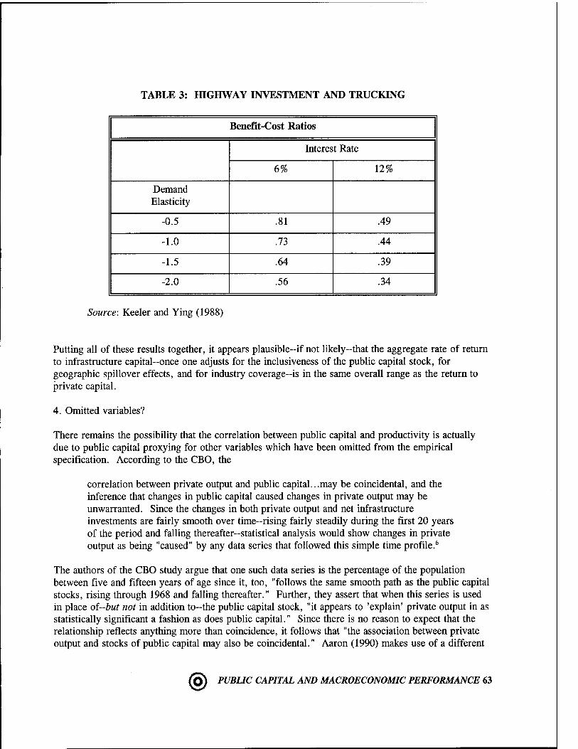
TABLE 3: HIGHWAY INVESTMENT AND TRUCKING

Benefit-Cost Ratios

Interest Rate

6% 12%

Demand Elasticity

-0.5 .81 .49

-1.0 .73 .44

-1.5 .64 .39

-2.0 .56 .34

Source: Keeler and Ying (1988)

Putting all of these results together, it appears plausible~if not likely-that the aggregate rate of return to infrastructure capital—once one adjusts for the inclusiveness of the public capital stock, for geographic spillover effects, and for industry coverage-is in the same overall range as the return to private capital.

4. Omitted variables?

There remains the possibility that the correlation between public capital and productivity is actually due to public capital proxying for other variables which have been omitted from the empirical specification. According to the CBO, the

correlation between private output and public capital...may be coincidental, and the inference that changes in public capital caused changes in private output may be unwarranted. Since the changes in both private output and net infrastructure investments are fairly smooth over time-rising fairly steadily during the first 20 years of the period and falling thereafter—statistical analysis would show changes in private output as being "caused" by any data series that followed this simple time profile.6

The authors of the CBO study argue that one such data series is the percentage of the population between five and fifteen years of age since it, too, "follows the same smooth path as the public capital stocks, rising through 1968 and falling thereafter." Further, they assert that when this series is used in place of—but not in addition to—the public capital stock, "it appears to 'explain' private output in as statistically significant a fashion as does public capital." Since there is no reason to expect that the relationship reflects anything more than coincidence, it follows that "the association between private output and stocks of public capital may also be coincidental." Aaron (1990) makes use of a different


data series-the yen/dollar exchange rate-to make essentially the same point. Aaron compares the predictive power of the public capital stock and the exchange rate and concludes that "the statistical support for the significance of an extremely improbable variable, the yen/dollar exchange rate, is just as strong as the support for a result the magnitude of which I regard as equally implausible."

The methodology used by the authors of the CBO study is to search for data series which will attenuate the relationship between public capital and output without providing any theoretical justification for the relevance of such variables. Indeed, the lack of theoretical motivation is viewed as something of a virtue. Yet without any theoretical rationale, any data series becomes admissible, and the ability of such researcher to find one or more data series to accomplish his goal will be constrained only by his desire to debunk a particular theory.

That having been said, it can be reasonably argued that the CBO and Aaron overstate their respective cases. It is true that various demographic variables-by themselves-perform in a manner similar to public capital in the statistical models. But what is also true is that when both the public capital and the demographic series are included in the models, the public capital series inevitably dominates; indeed, the demographic variables have no additional statistically significant explanatory power for output once public capital is included. It is also true that the yen/dollar exchange rate seems to "cause" productivity. But in order to eliminate the importance of the public capital stock for productivity, Aaron finds it necessary to not only include the yen/dollar exchange rate but also to convert to growth rates and to add dummy variables for 1966 and for 1974. It seems hardly surprising that with this much effort it is possible to overturn a particular empirical result.

Other researchers have taken what might be considered a preferable approach to the problem of omitted variables. Tatom (1991) argues that movements in the price of energy should be expected to have had an important impact on productivity overthe post-World War II period and, in accord with his view, adds the real price of oil as an additional explanatory variable in the aggregate productivity model of Aschauer (1989a). Tatom presents empirical results which seem to indicate that the addition of the oil price variable completely eliminates the importance of public capital in the statistical model, which leads him to conclude that "the hypothesis that public capital has a positive private sector marginal product cannot be supported."

Yet a closer, technical look at Tatom's methodology reveals a contradiction within his theoretical model. On the one hand, he assumes that firms maximize profit, so that oil should be employed as an intermediate input up to the point where its marginal product equals its real price. On the other hand, Tatom uses value added, and not total output, as his output measure. In this circumstance, oil- as an intermediate input-should "drop out" of his empirical model and should not directly influence productivity. Admittedly, there are other reasons why the steep increases in oil prices in the 1970's might have impacted on productivity-such as the rise in oil prices rendering the existing capital stock partially obsolete-but the point is that the way in which Tatom enters oil in his empirical model is theoretically unjustified. If one recognizes the above contradiction and correctly respecifies the model, one finds that oil price fluctuations and the public capital stock are key determinants of productivity. Specifically, the point estimate on public capital is equal to 0.23 and highly statistically significant (with an associated T-statistic of 5.75). Thus, Tatom's rather extreme results are to be seen as arising not because of the omission of oil prices but rather because of an incorrectly specified theoretical model.

64 PUBLIC CAPITAL AND MACROECONOMIC PERFORMANCE tfj)

Finally, it is not always the case that the inclusion of other variables diminishes the importance of public capital. Hulten and Schwab (1991b) use state level data for manufacturing and find little role for growth in the public capital stock in determining growth in total factor productivity. Yet Nadiri and Mamuneas (1991) find that when the capacity utilization rate and growth in the stock of research and development capital are added into the empirical model, the elasticity of output with respect to public capital is estimated at 0.29 and is statistically significant. The addition of the capacity utilization rate is justified since it captures movements in productivity over the business cycle. The growth in the stock of research and development spending has been shown to be an important determinant of productivity growth by a great number of researchers.

II. Public Capital and Macroeconomic Performance

The focus of the previous section of this review is on the importance of the public capital stock to productivity-variously, to labor productivity, to the productivity of the private capital stock, or to multifactor productivity (the amount of output produced by a certain combination of labor and private capital). The fundamental policy question is of the type: will a specific increase in the public capital stock (say, the capacity of the nation's transportation network) allow individual workers and firms in the economy to produce goods and services more efficiently?

While the primary question, as posed, is fundamentally one of microeconomic scope, it cannot be adequately answered apart from an overall macroeconomic environment. Any large scale public investment project will carry along with it macroeconomic effects on quantity variables such as the overall levels of output, employment, and private investment spending as well as price variables such as the general price level, wages, and interest rates. These quantity and price movements will be likely to affect the productivity measures listed above.

Consequently, this section of the review discusses the impact of changes to the public capital stock in a general equilibrium macroeconomic setting. Basically, there are two approaches to thinking about the effects of various shocks to the macroeconomy. Traditionally, the impact of public spending on the economy-public consumption or public investment-has been modelled in a non-market clearing setting, where the focus has been on the effects of government expenditure on the aggregate demand for goods and services. Under this approach, an increase in public expenditure raises the total demand for goods and services which, in turn, boosts the general price level. Given the current wage structure, the real wage is depressed-reducing unit costs of production-and profit-maximizing firms respond by increasing employment and output. The subsequent increase in incomes then supports an increase in consumption spending which then fosters a secondary increase in production and incomes. As this process continues ad infinitum, the initial increase in government spending can be seen to precipitate a much larger expansion in output-the multiplier process of traditional Keynesian models.

As described above, an increase in public investment spending would have the effect of dampening the productivity of labor. This conclusion rests on three standard assumptions of non-market clearing models: the (relative) fixity of the wage structure; the condition that profit maximizing firms will employ labor so as to equate the marginal product of labor to the real wage; and the principle of a diminishing marginal product of labor. Under this set of assumptions, as the real wage is depressed, firms find it optimal to increase employment until the productivity of the last worker hired falls to a level which just matches the lower real wage.


From the perspective of the current report, there are a number of difficulties with this traditional, non-market clearing approach. Perhaps most importantly, the conventional approach is better suited for studying the short run impact of public investment spending on output and employment rather than the long run effect of changes in the public capital stock on the level and/or the growth rate of output and productivity.

As a result, the discussion in this section of the report revolves around a market clearing macroeconomic model constructed along the lines of the model to be found in the work of Baxter and King (1993). Only the basic structure of the model will be sketched out here; details can be found in the papers cited above. In the model economy, there are two agents: a representative agent whose production and consumption decisions represent the private economy; and the government whose fiscal decisions regarding taxation and government expenditure are taken as exogenous by the representative agent.

The representative agent gains utility from consumption and suffers disutility from work effort. Importantly, he is bound by a time constraint-which implies that the total amount of time available must be expended at work or at leisure--and a resource constraint-which implies that after-tax income from the production of goods and services must be used for consumption, C, or for saving in the form of investment spending, I, on new private capital goods. This latter constraint can be represented as

C + I = (l-t)-Y + TR (9)

where Y represents income from production, t a tax rate on that income, and IK transfers (which, if negative, is taken to represent lump-sum taxes).

The government is similarly bound by a resource constraint which states that tax receipts must equal public investment spending, f , and transfers, 77?:

fY = IG + TR (10)

As specified, the public finance side of the model is simplified along two dimensions. First, consistent with the scope of the report, all public expenditure on goods and services is on investment goods; public consumption spending is ignored. Second, as the model admits an equivalence between transfer payments (or lump sum taxes) and debt issuance to finance a particular stream of government purchases of goods and services as in Barro (1974), it does not allow the possibility of debt finance of government purchases; however, we will discuss the likely impact of debt finance of public capital expenditures in a subsequent section.

The production of goods and services is accomplished by the utilization of labor, L, private capital, K, and public capital, K° in the Cobb-Douglas production function


Y = AftL, K,KG) = A-LVK(KGfKG <U>

As discussed in Aschauer (1989a), it is convenient to consider two possibilities regarding the degree of returns to scale in the production function. One is to allow for constant returns to scale over all inputs, private plus public, which is represented by the condition dL + 6K + 0KG = 1. In this case, if the private factors of production are paid according to their marginal products, the total output of goods and services will not be fully exhausted-there will be rents attributable to the public capital stock which would have to be appropriated by the private factors of production in some manner. Another case, which does allow for output to be fully exhausted when the private factors of production are compensated consistent with their marginal products, would be to allow for constant returns to scale across private inputs, 0L + BK = 1 and, consequently, increasing returns to scale over private and public inputs together. Presently, it is assumed that there are constant returns across private inputs.

When taken together, the individual resource constraints (9) and (10) and production function (11) yield the economy-wide resource constraint

C + / + IG = A-LVK(KGfKG <12>

or the standard output identity which states that output can be used for the purpose of consumption, investment in new private capital, or government spending (here, on new public capital).

The economy's equilibrium is characterized by the resource constraints above and by private sector efficiency conditions of two forms-one static and the other dynamic. The static efficiency condition requires that private sector choices of consumption spending and employment be such that any loss in utility due to increased work effort (due to foregone leisure time) be just matched by a gain in utility in the form of higher consumption. This condition can be expressed as

MUL = (l-t)-MPL-MUc (13)

where the left-hand side denotes the amount of utility lost due to an extra hour's work effort and the right-hand side denotes the amount of utility gained-as the product of the income generated by an extra hour's work effort, the after-tax marginal product of labor (l-t)MPL, and the marginal utility of consumption, MUC. It is important to recognize that in this expression the marginal utility of consumption and disutility of work effort are determined by the chosen amounts of consumption and work effort, while the marginal product of labor depends on the levels of employment, private capital, and public capital. For instance, an increase in consumption will tend to reduce the marginal utility of consumption, and an increase in work effort will tend to raise the marginal dis-utility of work effort at the same time that it lowers the marginal product of labor. Similarly, an increase in either the private or public capital stock will tend to raise the marginal product of labor.


The dynamic efficiency condition requires that private sector choices of consumption over time be such that any loss in current utility resulting from the decision to save and invest in new capital be matched by a gain in future utility as the proceeds from the investment are consumed. This condition is given by

MUC = (l-t)-MPK-MUc+1 (14>

where the left-hand side shows the loss in current utility and the right-hand side shows the gain in future utility as the product of the gain in future income, or the after-tax marginal product of capital (l-t)MPK, and the marginal utility of future consumption, MUC+1. Note that the marginal utility of current consumption is a function of current consumption and work effort, that the marginal utility of future consumption is a function of future consumption and work effort, and that the marginal product of capital is a function of the future levels of work effort and private and public capital stocks.

A. Direct and indirect effects of public capital spending

A key aspect of the model traced out above is that an increase in public investment and in the public capital stock can be expected to affect the levels of output and productivity in both direct and indirect ways. Consider, for example, a permanent increase in the level of public investment spending financed by an increase in lump sum taxes. The direct effect arises because changes in the public capital stock alter the level of output by making the private labor and capital inputs more or less productive; we can rewrite the production function as

Y = A-{KGfKG\LQLKQK\ = a{iV9*] (15)

to show that an increase in public capital (and an increase in a) works just like an increase in total factor productivity (or an increase in A). Conceptually, this effect of public capital is like an improvement to the transportation network which allows more output (e.g., delivery services in a certain period of time) to be obtained from given quantities of labor (e.g., truckdrivers) and private capital (e.g., trucks). This direct effect will be larger the larger is the value of the public capital efficiency parameter, 0KG. The indirect effect arises because an increase in the public capital stock will also affect the marginal products of labor and private capital which, in turn, influences the chosen quantities of the private inputs. Heuristically, an increase in the transportation network as above may also raise the marginal products of labor and private capital and consequently induce an increase in the levels of employment (e.g., more truck drivers are hired), private investment, and the private capital stock (e.g., to operate more trucks).

Baxter and King (1993) have computed the long run effects of an increase in public investment spending on output for a benchmark macroeconomic model. Table 4 shows the direct and indirect impacts on output. The direct effect rises with the value of the government capital productivity parameter, from zero in the case of unproductive government "investment" with 0KG = 0, to unity in the case where the government efficiency parameter equals the share of public investment in output,


TABLE 4: OUTPUT EFFECTS OF PUBLIC INVESTMENT

Multiplier Values AY/Af

0KG Direct (1)

K adjusts (2)

K, L adjust (3)

0.00 0.00 0.00 1.16

0.01 0.20 0.34 1.45

0.03 0.50 0.86 1.90

0.05 1.00 1.72 2.64

0.10 2.00 3.45 4.12

0.20 4.00 6.90 7.09

0.40 8.00 13.79 13.02

Source: Baxter and King (1993).

0KG = IG/Y = 0.05, and higher as government capital becomes more productive. Clearly, the government investment "multiplier," AY/AF behaves according to

Ay iG

< (>) 1 as Qvr < (>) —. AIG Y

(16)

Thus, the level of output net of government investment, Y -1° is left unchanged when the government capital efficiency parameter equals the share of public investment in output, while it decreases (increases) for lower (higher) values of the efficiency parameter. As long as the efficiency parameter exceeds (or equals) the current share of public investment in output, an increase in public investment spending can be said to be self-financing in the sense that there is an expansion of the level of output net of government resource use.7

The second and third columns of the table show the effects of the same increase in public investment spending taking into account the indirect effect on the private capital stock (the second column) and the private capital stock and labor together (the third column). Holding fixed the amount of labor services, the increase in output generated by an increase in public investment spending is seventy-two percent higher (e.g., 0.34 = 1.72 x 0.20) due to the induced increase in the marginal product of private capital and expansion in private investment spending. Consequently, the government spending multiplier exceeds unity as long as the efficiency parameter exceeds 0.029; government investment is now self-financing even if the efficiency parameter lies substantially below the share of public investment in output. Note also that these effects on output translate directly into effects on the productivity of labor since in columns (1) and (2) the level of employment is kept unchanged.


Finally, allowing for a response of private capital and labor yields an even larger increase in output (except at the highest value of the public capital efficiency parameter). Now, an increase in the public capital stock raises the marginal products of private capital (generating an increase in the private capital stock and output as time passes) and labor (generating an increase in employment and output). The reason for a smaller output effect (13.02 rather than 13.79) for the highest value of the efficiency parameter (0KG = 0.40) lies in the response of the consumer/worker in terms of his chosen level of work effort. At such a level of the government efficiency parameter, an increase in public investment is so productive and generates such an increase in wealth that the typical worker chooses to work less and to take more leisure time; with less work effort, the level of attained output is commensurately reduced.

The most significant aspect of the table is that government investment multipliers may quite easily exceed unity and, in this sense, government investment spending can be seen to be self-financing under a fairly wide range of values for the public capital stock efficiency parameter. Indeed, when both labor and private capital are allowed to expand, the public investment multiplier exceeds unity (AY/Af = 1.16) even when government capital is unproductive. This rise in net output represents an optimal response to the burden of higher government spending; the consumer/worker decreases consumption (by fifteen percent) but increases saving by more (by thirty-one percent) which requires an increase in work effort and output (by sixteen percent). Consequently, the fact that the government spending multiplier exceeds unity should hardly be seen as a rationale for increased government spending; unambiguously, the result of such higher public investment would be a decline in social welfare.

One set of estimates of output multipliers for nonmilitary public investment, military investment, and government consumption spending can be found in Aschauer (1990). This paper utilizes aggregate data for the United States over the period 1949 to 1985 to run regressions of the form

Y = a + ßr + yIG + ö-Z + vY <17)

where Y is output, f is public nonmilitary investment, t is a time trend and the a, ß, y, 8 are coefficients.8 The set of Z-variables varies, but includes public consumption spending, military spending, money growth, and the government budget deficit. In general, the estimates turn out to be consistent with the theoretical framework and with relatively high values of the public capital efficiency parameter 0KG. Specifically, the multipliers for nonmilitary investment are found to significantly exceed unity (ranging between 3.72 and 7.64) while multipliers for government consumption and military investment are found to lie below unity (ranging between 0.22 and 0.24 for government consumption and 0.21 and 0.66 for military investment).

In a recent contribution, Flores de Frutos and Pereira (1993) report an estimate of the elasticity of the growth rate of aggregate output with respect to the growth rate of the public capital stock for the United States over the period 1956 to 1989 to be equal to 0.99. The relationship between the output multiplier for public investment and this elasticity may be shown to be


e - -** • ™ (18) WKG AIG Y

In 1989, the net public nonmilitary capital stock equalled $1,941 billion (1987$) while gross domestic product equalled $4,837 billion, yielding a ratio of public capital to output of 0.40. Along with the elasticity estimate of 0.99, this implies an output multiplier for government investment spending of 2.475. This implied estimate is somewhat below the lowest estimate of Aschauer (1990), but de Frutos and Pereira employ a distinctively different methodology than Aschauer (1990), and so it is perhaps not surprising that the estimates are also somewhat different. The results of the two studies are alike, however, in that both estimates are consistent with the notion that public investment spending is productive and self-financing.

One implication of this discussion is that in order to accurately gauge the impact of public investment spending on output (or productivity) it will be necessary to go beyond the simple estimation of the output elasticity of public capital. While it is true that the output effects are generally larger the larger is the underlying output elasticity, it is also true that multipliers in excess of unity can be associated with output elasticities well below the level consistent with zero net use of resources by the government.

B. Short-run versus long-run effects of public capital spending

The multipliers discussed in the previous section pertain to the long-run impact of permanent increases in public investment, whereby output, private investment, and consumption achieve higher steady-state levels. In the transition to these higher long-run values, as the economy moves to a new steady state, different effects on these and other variables can be expected.

For example, Aschauer (1989b) provides a stylized dynamic model of the economy to capture the short-run and long-run effects of an increase in public investment on private investment (or the growth rate of the private capital stock). The empirical model is composed of two equations of the form

/ = c0 + <y/(-l) + c2-<j) + c3-IG + Vj (19)

(j) = c4 + c5-t + Cg-liL&T + c7*-ln£G + Cg-c« + v. (20)

where 4> is the marginal product of private capital, cu is the capacity utilization rate, and v7 and v^ are error terms. In this model, a change in the level of public investment has two separate effects on the level of private investment. First, an increase in public investment depresses the level of private investment since the representative agent in the economy is concerned with the national (public plus private) investment rate rather than the private investment rate per se. Accordingly, an increase in public investment which would raise the national investment rate brings forth an equal-sized reduction in private investment; from this perspective, public investment decisions turn out to be irrelevant to the rate of national investment and, in the empirical model above, the coefficient c3 would be


expected to lie in the neighborhood of -1. In fact, when the model is applied to data for the aggregate U.S. economy over the period 1953 to 1986, this coefficient is estimated to lie in the range of (-1.02, -0.72).

Second, the same increase in public investment raises the level of private investment as (r) the induced increase, over time, in the public capital stock raises the marginal product of private capital and (ii) the rise in the marginal product of capital provides an incentive for increased private investment spending. In the empirical model, the coefficients c7 and c2 would be expected to be positive; upon estimation, they are found to be in the range (0.79, 0.81) and 0.09, respectively.

Figure 3 illustrates the simulated impact of a permanent increase in public investment on private investment (measured as the growth rate of the private capital stock). The solid line depicts the actual historical time path for private investment. The dotted line shows a simulated time path for private investment where the level of public investment is raised by 1 percent (of the net private capital stock) during the years between 1970 to 1986. As is evident, the immediate impact of higher public capital expenditure is to reduce the level of private investment by nearly the same amount. This is because the direct, ex ante crowding out effect discussed above occurs immediately, while the indirect effect on private investment through the rate of return to private capital arises in subsequent years. However, by 1974, the simulated level of private investment climbs above the historical path and, thereafter, remains at a higher level. As a result of persistently higher investment, by 1986 the simulated level of the net private capital stock is 4.5 percent above its historical level.

Although these results are informative, it is important to recognize that the theoretical analysis in Aschauer's (1989b) study is based on a two period optimizing model. In such a model, it is only possible to consider the impact of a temporary increase in public investment since the additional output generated by any first period private or public investment must be consumed in the second period. In this sense, Baxter and King's (1993) model is better equipped to show the effects of a permanent increase in public investment spending. Figure 4 shows the impacts of such a permanent rise in public capital expenditure under the assumption of zero net resource use in the long run-that is, under the condition that the share of public investment in output is equal to the output elasticity of public capital (IG/Y = 0KG). In the figure, the circles denote the direct response of output, private investment, and labor input under the assumption that the marginal products of private capital and labor are unaffected; the triangles denote the total response of these variables when the indirect effects of public capital (working through impacts on the marginal products of the private inputs) are included.

As can be seen, the immediate impact of a rise in public investment is to raise output by approximately 0.6 percent (as one commodity unit equals 1 percent of initial output) and to boost employment by approximately 1 percent. The direction of the impact on private investment depends on whether or not the return to private capital is allowed to respond to the change in public investment. Holding fixed the rate of return to private capital, private investment tends to decline by a small (nearly trivial) amount; a decline because the rise in public investment represents a drain on the resources available for private consumption and private investment, and by a small amount because the resource drain is highly persistent and the representative agent has little cause to reallocate his lifetime resources intertemporally.


CD 00

CO CO

o CO

- t=

p

CO CO

in u>

- a

- 81

to to

CO m

'CU S- 3 0D


Thus, the immediate impact of the increase in public investment is to lower, and not to raise the level of labor productivity since the positive output response of 0.6 percent is outweighed by a positive employment response in excess of 1 percent. The limited extent of the rise in output is the outcome of a fall in private demand for output as private consumption falls by approximately 0.4 commodity units and private investment changes by somewhat less than 0.1 commodity units.

As time passes, however, the level of labor productivity begins to rise in both economies as output continues on an upward path and employment declines (immediately in the case of the triangle economy and after three or four years in the circle economy). In both economies, the level of labor productivity is higher in the new steady state-by 1 percent in the triangle economy, with output rising by 1 percent and labor input returning to its original level, and by approximately 1.8 percent in the circle economy, with output rising by 2.6 percent and employment rising by 0.8 percent.

One empirical implication arising from this discussion is that it is critically important to distinguish between the short-run and long-run effects of public investment on productivity. Above, the output elasticity of public capital is positive and so public investment is productive. Nevertheless, the temporary impact of an increase in public investment is to lower rather than raise the observed level of the productivity of labor. In the short run, labor input rises and private consumption falls-both rather dramatically-as the representative agent responds to the drain on the economy's resources resulting from the increase in public investment spending. Only over time, as the rise in public investment represents a smaller and smaller net drain on the economy's resources, does the level of labor productivity rise along with public investment and the public capital stock.

C. Level versus growth effects of public investment spending

In the traditional neoclassical model of economic growth (e.g., Solow (1956)), public policies such as a change in the rate of public investment spending can have effects on the long-run level-but not the long-run growth rates-of output and productivity. Public policies can influence the growth rate of output or productivity only in the transitional phase as the economy moves from one to another long- run equilibrium (or steady-state). In particular, there is no possibility of a linkage between the rate of public investment and long-run economic growth in this class of models since the latter is completely determined by exogenously determined factors such as population growth and technological progress. The simulation results presented in Figure 4 fall into this category as the permanent increase in public investment spending merely results in an increase in the long-run level of output; the growth rate of output gradually tails off to zero as time passes.

More recently, a new class of economic growth models has been developed (Romer (1986), Rebelo (1991)) in which public policy changes can impact the long-run rate of growth of output or productivity. The key feature of this class of model is that the net return to private capital stocks is bounded away from zero, which puts certain requirements on the form of the production function. Consider, for example, the Baxter and King (1993) specification of the production function

Y = F(L, K, KG) = A-L*LK\KGfKG (21)


A. Public Investment 9<odc B. Direct Output Response

o O

C. Output

3 1.5

08

06

D. Consumption

• a-» •

c -> 02 •

• X • fc E o o

0

-02

V

• •

^ A

-0.4

J1K

• *

2 4 S 8 10 12 14 16 18 20

Years

E. Investment F. Laoor Input

o E E o o

a6 .•""

as • • • 0-4 •

• 0.3 •

• 02

4»

m

0

•

0 2 4 S 8 10 12 14 16 18 20

Years

0 2 4 6 8 10 12 14 16 18 20

Figure 4

(S) PUBLIC CAPITAL AND MACROECONOMIC PERFORMANCE 75

along with the auxiliary condition that the government invests in public capital so as to maintain a constant ratio of public to private capital

<h = 9. (22) K

Substitution of equation (22) into equation (21) then allows

Y = A,^

>KG,L

QLK

QK+

QKG ^^

so that the output elasticity of private capital is equal to 0K + 0KG rather than 0K since the private decision to increase the private capital stock brings forth an increase in government capital which is itself productive. Now, in the simulations contained in Baxter and King (1993), the sum of the output elasticities of private and public capital is fixed at 0.25, reflecting the assumptions of a sharply diminishing returns to private capital (with 0K = 0-20) and zero net resource use of public capital (with 0KG = 0.05). But suppose that private capital exhibited a less severe degree of diminishing returns and/or public capital were extraordinarily productive so that 0K + 0KG = 1. Then the production function can be written as

Y = A-$KG

'LQL

K (24)

which implies that the marginal product of private capital will be constant and equal to

dK

In this instance, an increase in the steady state ratio of public to private capital (which requires an increase in the public investment rate) will raise the returns to private capital, stimulate private investment, and raise the long-run growth rate of output and labor productivity.

It is useful to compare the paths for output (or productivity) for an exogenous growth model (similar to Baxter and King (1993) yet with a fixed labor force) and an endogenous growth model as sketched out above. In the former (0K + 0KG = 0.25 < 1) economy, an increase in the public investment rate will cause a temporary increase in the rate of growth of output and productivity and a permanent, but bounded increase in output and productivity levels. In the latter (0K + KG = 1) economy, however, an increase in the ratio of public to private capital and the associated increase in public investment will cause a permanent increase in the growth rates of output and productivity and an unbounded increase in output and productivity levels.


Clearly, then, in order to gauge the long-run effects of an increase in public investment it is necessary to determine if the economy is better characterized by an exogenous or endogenous model framework. To date, only a limited amount of work in the area of research on public capital has been directly related to this question. Kocherlakota and Yi (1992) study the long-run effects of six government policies (changes in tax rates, in money growth, in tariff rates, in military and nonmilitary equipment investment, in nonmilitary structural investment, and in governmental educational expenditures) using aggregate time series data from 1917 to 1985. They find that only two policies-permanent changes in structural investment and educational spending-have an impact on the long-run economic growth rate. In particular, the estimates show that a one percentage point increase in the public investment rate implies a permanent increase of 2.4 percentage points in the growth rate of output. Hulten and Schwab (1992) look for evidence of spillover effects from public capital on private capital accumulation using regional manufacturing data over the period from 1970 to 1986 and conclude that the evidence "lends little support to the argument that public capital externalities (whereby an increase in public capital raises the returns to private capital) are an important engine of growth." Holtz-Eakin (1993) includes public investment in an exogenous growth framework and uses state-level data over the period from 1970 to 1986 to estimate the impact of changes in the rate of public investment on economic growth. He concludes that from "the perspective of public sector capital accumulation, a robust bottom line emerges: the data do not assign an important quantitative role in explaining the growth patterns of states."

D. The financing of public investment spending

The previous discussion assumes that the financing of public investment spending is accomplished through lump-sum or non-distortionary taxation. This, of course, is an unrealistic assumption- typically, public investments are financed through increases in user fees or tax rates on labor and capital income.

In a neoclassical setting, the analysis in Baxter and King (1993) suggests that the economic impacts of changes in public investment spending will be quite sensitive to the choice of means of finance. In the neoclassical model, an increase in tax rates will reduce the incentives to work, save, and invest which, in turn, will typically reduce the positive effect of government spending (productive or otherwise) on output. For example, Baxter and King (1993) simulate the impact of permanent increases in unproductive government spending financed by an increase in income tax rates. In the benchmark model, they find that the government spending multiplier is reduced from AY/AG = 1.16 under lump-sum taxation to AY/AG = -1.10 and conclude that "evidently the public finance decision is central to the effects of government purchases."

In an endogenous growth setting, Barro (1990) shows how the economic growth rate responds to tax- financed changes in government spending. In his model, a rise in the level of productive government spending raises the marginal product of private capital, stimulates private investment, and boosts economic growth. However, the increase in government spending also requires a rise in the tax rate on income which, in turn, reduces the after-tax return to capital and acts to deter investment and growth. At low levels of government spending, the productivity enhancing effect of government spending dominates the tax effect and the after-tax marginal product of capital rises. This rise in the return to investment stimulates private capital accumulation and raises the economic growth rate. But at sufficiently high levels of government spending, the tax effect overwhelms the productivity effect, the after-tax return to capital is depressed, and private investment and the growth rate decline. In


Barro's (1990) model, the economic growth rate is maximized when the ratio of productive public expenditure to output equals the output elasticity of government spending, or when the marginal product of public expenditure equals unity.

The important implication is that the impact of increases in inherently productive public sector inputs on the level and growth rate of output depends on the means of financing such spending. Consequently, the finding that public capital is productive is,then, hardly sufficient to ensure that boosting public investment spending will raise the long-run level of output or stimulate long-run economic growth.

III. Proposed Research Strategy

In this section, a research strategy is laid out which focuses on the long-run effects of public capital on the level or growth rate of output (or productivity). Two models are proposed. The first is a neoclassical growth model with regional spillover effects of public capital. In this model, changes in local or regional public investment influence the level of output in the long run and the growth rate of output in the short- and intermediate-runs (i.e., in the transition phase between long-run equilibria). The second is an endogenous growth model where public capital is financed by an income tax. In this model, changes in the public capital stock alter the long-run growth rate of output as long as the government sector is not choosing the level of public capital in an optimal fashion.

These two models are intended to address a number of the statistical and theoretical considerations contained in the previous sections of this review, such as: spurious correlation; the magnitude of effect of public capital; the endogenity of the public capital stock; direct versus indirect effects of public capital; short-run versus long-run effects; and level versus growth effects of public capital. Table 5 briefly describes how the proposed research strategy addresses some of these considerations.

A. The neoclassical model with public capital and regional spillovers

The research strategy sketched out here synthesizes recent work in the economic growth literature as represented by Mankiw, Romer, and Weil (1992), Brum (1992), and especially Chua (1992). The thrust of the approach is to relate productivity levels to investment rates and to capital stocks in a neoclassical growth model setting (as in Mankiw, Romer, and Weil (1992)), to introduce public capital (as in Brum (1992)), and to allow for regional spillover effects (as in Chua (1992)). In each of these aforementioned papers, evidence has been gathered on the appropriateness of the neoclassical economic growth model when it is augmented to include human capital, public capital, or regional spillovers. Mankiw, Romer and Weil (1992) obtain estimates of the output elasticities of physical and human capital which substantiates the appropriateness of the neoclassical model; in particular, they find evidence of a conditional convergence of a country's output per worker to a long run or steady state value. In the same sort of setting, Brum (1992) finds evidence that the output elasticity of public capital is comparable to that of private capital. Chua (1992) obtains evidence of regional spillover effects from private capital. The high degree of success of the previous empirical work in this area of investigation allows a presumption of success for the proposed research strategy.


TABLE 5: RESEARCH STRATEGY CHARACTERISTICS

Consideration Research Strategy Characteristic

Spurious correlation due to nonstationarity of data

Relate productivity levels and growth rates to public investment rate

Spurious correlation due to omitted variables

Include state-specific influences on productivity other than public capital

Endogenity of public capital stock due to correlation between per capita income and public capital stock

Relate public capital stock to public investment and private investment rates and to population growth

Magnitude of estimate of return to public capital stock

Estimate degree of external effect across state boundaries

Short-run versus long-run effects

Estimate rate of convergence of productivity to change in public investment

Level versus growth rate effects Estimate returns to scale in private production

Consider the level of per worker output in a particular state economy (y) and the average level of per worker output in the associated regional economy (y). The regional economy may be defined by the Bureau of Economic Analysis divisions (of which there are eight), by the Bureau of the Census regions (four) or divisions (twelve), or by groups of bordering states (e.g., the region for Illinois would be composed of Illinois, Wisconsin, Iowa, Missouri, and Indiana). The basic intent is to estimate the extent to which the public capital stock of a region is a determinant of the productivity of individual states within that region (say, Massachusetts).

Let the production function for a particular state be given by

Y = A-flL, K, KG) A.T} ®K ®KG

K^K

KCT ^KG (26)

While this particular specification of the production function involves only one form of private capital and one form of public capital, it is a straightforward exercise to incorporate additional types of capital in the analysis.

In per worker terms, the production function (26) may be rewritten as

6*-» 9* y = A-k Kkg (27)


where lower case letters are used to denote the per worker analogue of the respective upper case variable. Next, allow the level of multifactor productivity in a particular state to be a positive function of the public capital stock of the region as in

A = kg' (28>

Of course, other state or regional factors {e.g., industrial structure, weather, demographics) may also be important determinants of total factor productivity. These factors, presently omitted to focus attention on the role of public capital, can be readily included in the actual empirical analysis.

Substitution for total factor productivity (equation (28)) in the production function (equation (27)) then yields

y = kW°W (29>

The standard neoclassical growth model assumes a constant rate of growth of the labor force and a constant depreciation rate on physical capital. Here, the labor force growth rate and the depreciation rate on private and public capital are denoted by X and 8, respectively. For simplicity of exposition, it is assumed that population growth rates are identical for individual state economies and for the associated regional economy. This assumption may be relaxed in the empirical analysis. Similarly, it is assumed that the depreciation rates on private and public capital are identical.

The private and public capital stocks, specified in per worker terms, will accumulate over time at rates given by

* = oKy - (X+Ö)k (30) dt

and

^ = oKGy - (X+Ö)kg (3D

where aK and aKG are the shares of state output which are invested in private and public capital, respectively. Note that for a fixed rate of (private or public) investment, the growth rate of the (private or public) capital stock will be lower the higher is the labor force growth rate, X, or the physical depreciation rate, 8.

Now, average output per worker in a particular region is given as the geometric average of output per worker in the individual states comprising the region. Thus,

80 PUBLIC CAPITAL AND MACROECONOMIC PERFORMANCE £<))

1 K

lay = -i]Tlrry (32)

Rewrite the state level production function (29) in logarithmic form and substitute to get

_ i R _ ty = ^E t6**+ ®KGkg + eksi

K 1

In similar fashion, define k and kg as the geometric average of the private and public capital stocks in individual states of the associated region. Then average regional output may be seen to be given by

lny = e^lnÄ + {QKG+z)\nkg (34)

Thus, the elasticity of average regional output with respect to public capital is equal to 0KG + e while the elasticity of state level output with respect to public capital is 0KG; average regional output and productivity levels internalize the externality associated with the regional public capital stock. Note that by direct extension-now treating regional economies rather than state economies as the basic unit of observation-it is possible to obtain an analogous expression for average national output per worker as in

]nyN = ö^lnA" + (QKG+e+r\)\nkgN (35)

where yN, k", kgN are the geometric averages of regional output and private and public capital stocks per worker and t\ measures the external effect of the national public capital stock on regional output. Since the output elasticities increase with the level of aggregation, from 0KG at the state level to 0KG + e at the regional level and finally to 0KG+ e + rj at the national level, the conceptual framework is consistent with the geographic pattern of elasticity estimates which were presented in Table 2 above.

The evolution of the regional private and public capital stocks can be determined as follows. As with output, the average private capital stock is given by

R

\ok = -Yhik (36)

Differentiating this last expression yields

(8) PUBLIC CAPITAL AND MACROECONOMIC PERFORMANCE 81

R 1 dk _ J_^ ^dk (37) I dt Ri k dt

After substituting in equation (37) from the individual state capital accumulation equation (30) and rearranging, we obtain

^ = n.v - tt+Ätf (38) — = Ojj - (A+6)&

where

s.-iE'^xl) <M> i?V & y

is the regional private investment rate. Note that a precise calculation of the regional investment rate requires data on private capital stocks of individual states.

By a similar calculation, the evolution of the regional public capital stock is given by

^ = 0^ - (A+6)^ (40) at

where

■±t°*tix$> (41) °KG Rr " *8 y

is the regional public investment rate. As with the regional private investment rate, an exact calculation of the regional public investment rate will require state level data on public capital stocks.

In this neoclassical model, the economy will achieve a steady state or long-run equilibrium when the net private and public capital stocks per worker are constant, or when

82 PUBLIC CAPITAL AND MACROECONOMIC PERFORMANCE ($)

M=dkg = dk = dkg=0 (42)

dt dt dt dt

Under these conditions, the steady state capital stocks for the regional economy can be computed as

fop = ^°KG + V-QKG-*)^ - fr(*+S) (43)

—,. lno^ + O^kid) - ln(A+6) ]nkgss = *° *®—1 (44)

1-

QK-

QKG~

C

and, by substitution into the regional production function, the steady state level of regional output is obtained as

]nyss = (6^+e^+E)lno^ + W " (yQgg+e)lnq+5) (4g)

Inspection of equation (45) indicates that the level of regional output increases with increases in the regional ratio of public to private capital and with the regional public investment rate and decreases with increases in the population growth rate or the physical depreciation rate on capital.

Solutions for the steady state capital stocks and output for an individual state can be derived in a similar fashion. These are:

Injfe« = lnqgG+(1-ejcG)ln<l)+ elno^+ö^ehKt) ln(A+5) (46)

1-Ve^ (1-6,-e^Xl -6,-6^-e) l-ve^-e

]nkgSS = fo°KG+QK]n,b+ elno^+e^kKJ) ln(A+6) (47)

1-Qr6KG C1-0*-0«^1-6*"6«?-8) 1_W~E

(A) PUBLIC CAPITAL AND MACROECONOMIC PERFORMANCE 83

= 9^ +(V6rG)mo*G^ elno^-e^eliMj)

i-VV a-8,-6^(1-e,-ero-e) (48)

((ö^e^xi-e^-e^-e)^) +

(1-0^-0^(1-0^-0^-0

The level of output per worker in an individual state can be seen to increase with increases in state- specific investment rates and to decrease with increases in the population growth rate and the depreciation rate. As a result of the spillover effect of regional public capital, however, the level of state output also increases with increases in the regional public investment rate and in the regional private investment rate. On a cursory look, the latter effect might seem surprising since there are no direct spillover effects from regional private capital built into the model. However, note that an increase in the regional private investment rate will induce an increase in the steady state level of the regional public capital stock which, in turn, will raise the level of output in any given state in that same region.

1. Empirical implementation

Consider the empirical version of the theoretical equation (48) for the output level of a particular state:

hiy" = a + bZ + qm^ + cJnoKG .+ c3ln<j> + cJnoKG + c5ln(A+6) + vy (49)

where a is a constant term, the Zy variables denote state-specific factors affecting the steady state level of output (e.g., resource endowments, climate, or overall fiscal stance as given by government consumption and/or tax rates), the c, coefficients are as specified in the theoretical model above, and vy is a random error term.

This model can be estimated by ordinary least squares, with the structural coefficients (0K, 0KG, e) retrieved from the estimates of the ct. For example, we could obtain an estimate of the output elasticity of the private capital stock as

6 = !± (50) * c3

where hats denote estimated values of the relevant coefficients.

84 PUBLIC CAPITAL AND MACROECONOMIC PERFORMANCE ß)

Note, however, that (ignoring the constant a and the &,) the model involves three parameters to be estimated (0K, 0KG, e) from five coefficient estimates (c„..., c5). Consequently, estimation by ordinary least squares will not yield a unique set of parameter estimates.

Alternatively, the model can be estimated by non-linear least squares in unrestricted and restricted form. The unrestricted version of the model would involve setting

e* . = dK+Ql C, = — C = — C- = - (51)

and leaving c4 and c5 unrestricted. The restricted version of the model would involve setting Cj through c3 as above but also setting

c _ -OK* C _ (Q

K+

QKG)V-VK-QKG-Z)+

* (52) 4 a-veâ-ve^-e)' 5 (l-eê^xi-eê^-e)

In the unrestricted model, there is an equal number of parameters and independent variables, while in the restricted model there are two fewer parameters than independent variables. Thus, a likelihood' ratio statistic, distributed as a chi-square random variable with two degrees of freedom, can be computed and a test performed to determine the appropriateness of the restrictions implied by the model.

A gain in the efficiency of the parameter estimates can be obtained by jointly estimating the output equation given above along with an equation for the public capital stock given as

]nkgss = d + e-ZKG +/1ln<|> +/2lnoTO + /3ln<j> + f^ö KG +/5ln(A+ö) + vkg (53)

where of is a constant term, the Zkg are state-specific variables which influence the steady-state public capital stock, the j^ are coefficients specified in the theoretical model above, and v^ is an error term. The model composed of the output and public capital equations involves ten independent variables (apart from the constant terms and the Zy and Zkg variables) and three parameters to be estimated. Consequently, a likelihood ratio test with seven degrees of freedom can be performed to judge the adequacy of the model.

2. Transition equations for output

As discussed in a previous section, in recent years a number of economists have turned away from the neoclassical growth model in favor of endogenous growth models. The attraction of endogenous


growth models is that they allow an economy to grow indefinitely rather than force the economy to converge on a particular steady state level of output. The specific assumption that gives endogenous growth models this attractive feature is that there are "non-diminishing returns to reproducible factors of production."

In the present neoclassical model with public capital spillovers, the regional economy will have diminishing returns to reproducible factors of production (private and public capital) as long as the sum of the output elasticities of private and public capital (including the latter's spillover effect) exceeds unity, or (l-0K-0KG-e) > 0. In this situation, the regional economy will converge on the steady state output level at an associated geometric rate equal to (l-6K-6KG-e)(k+8). Suppose, however, that the public capital spillover effect were sufficiently large that e = (1-0K-0KG)- In this alternative situation, constant returns to the reproducible factors arises and the regional economy will grow at a unceasing rate. So the estimate of e is important not just for determining the true output elasticity of public capital but also for determining whether a change in the public investment rate will induce a temporary or a permanent increase in economic growth.

It would appear that the previously obtained estimates of 0K, 0KG, and e can provide sufficient information for deciding in favor of the neoclassical growth model or the endogenous growth model. But the empirical analysis sketched out above is predicated on the assumption that the various state and regional economies have already achieved their steady state levels of output per worker. Since any one, or more, of these economies might be on the transition path to their ultimate steady state positions, the parameter estimates obtained from the above model may turn out to be inaccurate.

Fortunately, it is possible to derive an equation which specifies the level of output at any point in time along the transition path to the steady state. This equation can then be estimated using data on the observed level of actual output rather than the unobserved level of steady state output. For a particular state economy behaving according to the model of the previous section, the level of output at any point in time can be shown to be given by

lny = lny0 + (l-e^Ony"-^ - («^-e^W'-lnyo) (54)

where y0, y0 are state and regional output levels in some initial year, yss and y" denote the respective steady state output levels which were given above as

k_M = (QK+dKG+e)hi^KG + ö^lnÄ - (e^e^+eMA+d) (55)

86 PUBLIC CAPITAL AND MACROECONOMIC PERFORMANCE (Ä)

d^n^>+(QK+dKG)\naKG e\no K-QKe\nfy

(56)

(1-6,-6^(1-6,-6^-e)

and where ßx and ß2 are parameters which determine the rate of convergence of output to its steady state level.

The elimination of the (unobserved) steady state levels of state and regional output allows the specification

fry = £(y0> yv ♦» °KG> *> °KG> X+6

> PI» P2) (57)

which, as before, can be estimated by non-linear least squares in unrestricted and restricted form. As there are five parameters to be estimated (0K, 0KG, e, ßu ß2) and seven independent variables there are two degrees of freedom to conduct a test of the appropriateness of the restrictions.

Further, it can be shown that the convergence parameters are not free parameters but rather are equal to

Pi = (l-e^-e^XA+ö); ß2 = (l-e^-ö^-eXA+ö) (58)

so that the model can be estimated in an even more restricted form with only three parameters to be estimated (0K) 0KG, e) with seven independent variables. Acceptance of these restrictions, along with a positive (yet sufficiently small) estimated value for the parameter e, would appear to offer strong confirmation of the appropriateness of modeling the economy along neoclassical lines augmented by public capital spillovers.

B. An endogenous growth model with public capital

In this section, an endogenous growth model is constructed in order to consider the long-run effects of public capital on economic growth. The model is similar to that of Barro (1990) but allows the public capital stock, rather than the flow of public expenditure, to enter the private sector production function.


In this model, the representative agent maximizes a constant intertemporal elasticity of substitution utility function over an infinite planning horizon as given by

{ l-o

where c represents consumption, -a the constant elasticity of the marginal utility of consumption, and p the rate of time preference.9 The agent has access to a Cobb-Douglas production function

y - kW*K m

where y is output, k is a broad measure of private capital (inclusive of tangible and human capital), and kg is public infrastructure capital.10 All variables are expressed in per worker terms. Thus, the production function exhibits constant returns to scale across the private and public capital inputs, but increasing returns to scale across raw labor and capital. The model ignores technological progress, population growth, and depreciation of private or public capital in order to bring out the essential points in the clearest manner.

The government purchases and maintains the stock of public capital which enters as an input to the private sector production function (60). At an initial point in time, the government is viewed as choosing a particular level of public capital, kg0. The initial purchase of government sector capital is assumed to be financed by the sale of perpetuities at a coupon rate of r percent. Subsequently, the government is taken to maintain a particular ratio of public to private capital

* = M (61) k

which requires an increase in the public capital stock over time at the rate

kg = ykg

where y is the rate of growth of the private capital stock.

88 PUBLIC CAPITAL AND MACROECONOMIC PERFORMANCE (gj

It is assumed that the government levies a tax on private production at rate t for the purpose of financing (i) the on-going public expenditure needed to maintain the public capital stock ratio against growth in the private capital stock and (ii) the interest payments on the initial stock of debt. Accordingly, the government budget constraint is

£#o + [^8 e~rsds = ft-y e rsds. (63)

where s denotes time.

Given steady state growth at the rate 7, the government budget constraint reduces to11

r-kg0 = t-y0. (64)

The representative agent maximizes utility as given in equation (59) taking the public capital stock and the tax rate as beyond his influence. The maximization of utility is subject to a standard resource constraint which determines the level of private capital accumulation as the difference between after- tax income from production and private consumption12

<W-e* - r (65) k = (l-t)kKkg VK - c

In this environment, the steady state equilibrium involves a common growth rate of consumption, public and private capital, and per worker output given by

Y = -Ki-OM»1"6* - p]. (66) a

Evidently, the common growth rate of consumption, capital, and output depends positively on the ratio of public to private capital and negatively on the tax rate. In order to determine the net effect of government capital accumulation on economic growth, it is necessary to eliminate the tax rate from the growth rate expression in equation (66).

This elimination of the tax rate is accomplished in the following manner. First, note that in equilibrium the government's maintenance of a particular ratio of public to private capital, 4>, implies that private sector output may be written as


y = k\g^ - k\k^^ = k^ (67)

As a further equilibrium condition, the representative agent must be willing to hold the available stocks of debt and private capital. Consequently, the interest rate on government perpetuities must equal the net of tax return to private capital, so that

i-e* (68) (.i-WA

The steady state budget constraint in equation (64) and the level of output in equation (67) may be solved for the tax rate as a function of the interest rate on public debt and the public capital stock ratio

t = rV* (69)

which, after substituting into equation (68) allows us to obtain the steady state equilibrium interest rate as

r = 9^ (70) 1+6^'

Finally, from equations (66) and (70) we get the solution for the growth rate of per worker output as a function of the public capital ratio:

Y = 1[ W"' - p]. (71)

Figure 5 traces out the relationship between the growth rate, y, and the ratio of public to private capital, <j>, for a particular value of the output elasticity of private capital, 0K The growth rate initially rises with the ratio of public to private capital, reaches a maximum, and then falls toward zero. The intuition, similar to that described above in the model of Barro (1991), is straightforward. Consider an increase in <j> induced by a marginal increase in the public capital stock. For a given tax rate, the increase in the ratio of public to private capital increases the after- tax marginal product of capital in the amount13


o

CD

O

CO

o

[^

o O

CD b O

"5 LO D_ O o

o IT)

"NI- _u 0>

3 CO -Q Ml

13 to ü_

rO O

CM

O

o

q O

CO r^ CD m ro CSJ

ip.MOjß XjlAQOnpOJcJ

(3) PUBLIC CAPITAL AND MACROECONOMIC PERFORMANCE 91

Taken alone, this increase in the marginal product of capital would be conducive to growth. However, the increase in the public capital stock also requires a rise in the tax rate which, in turn, reduces the after-tax return to capital in the amount

4(1-')/*], _ (i-e,M> ' (72) db t = t l+e^

4(i-^], _= M~* (73)

d<\> fk=fk (l+e^)2'

This decrease in the after-tax marginal product of capital, when taken by itself, would deter growth. At low levels of <f>, the productivity effect in equation (71) dominates the tax rate effect in equation (72), and the after-tax marginal product of capital rises. This rise in the return to investment, in turn, stimulates private capital accumulation and raises the growth rate. But at sufficiently high levels of <j>, the tax effect overwhelms the productivity effect, the after-tax return to capital is depressed, and private investment and the growth rate decline.14

Specifically, the growth rate of consumption rises with the ratio of public to private capital from a minimum of 7min = -pia to reach a maximum of

Y 1 26r „ ,1-0 max x r n K/-X n \L u.

a [ Ca-e*re* - Pi- <74>

Equations (72) and (73) can be used to show that the maximal growth rate of per worker output, y™3*, corresponds to a ratio of public to private capital given by

^max = Q^l [■ K] (75) 9*


When the tax rate function is evaluated at the ratio of public to private capital which maximizes the economic growth rate, <^max, we obtain

Combining equations (74) and (75) then yields the result that the economic growth rate is maximized when the government chooses a ratio of public to private capital so as equate the after-tax marginal product of private capital to the marginal product of public capital:

(!-#*=/, (77)

where fx denotes the marginal product of input x (x = k, g) and we have used the fact that for the Cobb-Douglas specification of the production function the output elasticities of private and public capital are equal to 0K and 1-0KG, respectively.

It is instructive to compare the decentralized steady state equilibrium derived above with the centralized steady state equilibrium obtained by having the government choose not only the public capital stock but also the time path for private consumption. This will generate an alternative relationship between the growth rate of per worker output and the public capital ratio since the government will take into account the external effect of any induced increase in public capital on the marginal product of private capital. In the present case, the relevant resource constraint is given by

k = (i-m1-*«- c (78)

which differs from the resource constraint for the decentralized problem in that the production function is given by

y = k*'-°< <">


since the government internalizes the response of public capital to movements in private capital which is needed to maintain a particular value of <f> = kg/k. In this case, after solving for the centralized economic growth rate, we obtain

Y = I[i!^ - p]. (80) ö (1 +*)

Figure 6 traces out the relationship between the growth rate and the public capital ratio for a particular production function (the solid line) and compares it to the decentralized case (the dotted line). Just as with the decentralized case, the growth rate initially rises, reaches a maximum, and then declines with the capital stock ratio. In the present case, however, the economic growth rate is maximized at a value of

rax = ire^i-e*)1-9* - p] (8D

and at a ratio of public to private capital given by

<j)max = ^ 9^ (82)

which turns out to be equivalent to the condition that the pre-tax marginal product of private capital be equated to the marginal product of public capital:

fk fg- (83)

A comparison of the decentralized and centralized outcomes reveals two informative results. First, equations (71) and (80) show that the centralized growth rate is uniformly higher than the decentralized growth rate by the percentage point amount

_ q-e^d)1-9* m Y Y 0(1+40(1+0^)'


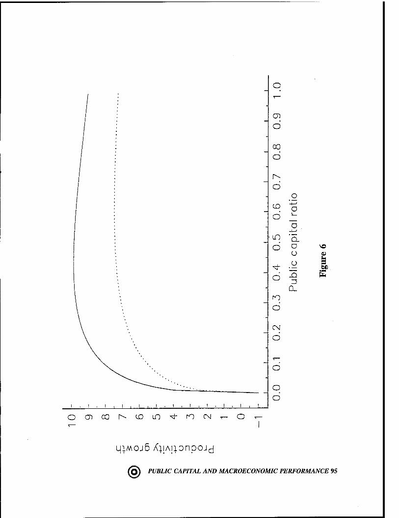
o

/ -

U]

/ d

/ CO

/ O

'

1 -

d

CO

d

■LO

d

d P

ublic

capital

ratio

Fig

ure

6

rO

- d

CM

- d

N^ d

I f 1,1,1.1

'"•-: o d

i i , i , i 1 1

c ) en CO N CD Lf) ^- rO CM T— o ■c—

1

q^.MOjß Ä^iAiionp OJd

(j$S PUBLIC CAPITAL AND MACROECONOMIC PERFORMANCE 95

This result arises because in the centralized case the government takes account of the positive effect of public capital on the return to private capital, which results in a higher chosen level of private investment spending and higher growth.

Second, by comparing equations (75) and (82), it is evident that the growth-maximizing ratio of public to private capital is higher in the decentralized case than in the centralized case by a percentage amount equal to

<|)ma*-frmax = (1-9*) (85)

In the centralized equilibrium, the government accumulates public capital in an amount that generates an external benefit to private capital which just offsets the depressing effect of a higher tax rate, and the maximal growth rate arises where the pre-tax marginal product of private capital equals the marginal product of government capital. In the decentralized case, however, the external benefit is overlooked by the representative agent, and the maximal growth rate arises where the after-tea marginal product of private capital matches the marginal product of private capital. This implies that in the decentralized case there is too little private capital accumulation for a given level of public capital accumulation which, in turn, results in too high of a ratio of public to private capital.

So far, we have looked for public capital ratios which maximize steady state growth within a particular governmental jurisdiction. However, much of the empirical work on economic growth is undertaken on the basis of cross-sectional data at the state, regional", or international levels. It may be expected that production functions may vary across jurisdictions and, as a consequence, that different levels of the public capital ratio may turn out to maximize economic growth.

To investigate this point further, consider a situation where there are a large number of different governmental jurisdictions indexed by i = 1, 2, 3,.... The production function in each jurisdiction is then given by

y. = *eV8'' (86) ' i i

Let each government choose the (centralized) growth-maximizing ratio of public to private capital, expressed as

max _ (1"V (87) 1 6.

96 PUBLIC CAPITAL AND MACROECONOMIC PERFORMANCE (rfo

which from equation (81) can be seen to generate the maximum growth rate in jurisdiction i as

?f* = hiß^Ki-e^ - p]. (88)

For purposes of comparison, it is useful to rewrite this result as a function of <£,, as in

.max icj).1^ (89) Y = -[— - p]

1 a l+<p

Figure 7, which contains a graph of equation (89), shows how the growth rate varies as the growth-maximizing ratio of public to private capital varies across jurisdictions. (For comparison, the decentralized and centralized steady state relationships between growth and the public capital ratio-for a particular production function—are also shown as the dotted and dash-dotted curves, respectively). In the limiting case where public capital is unproductive~or, where 0Ki = 1 and </>, = 0-the growth rate equals (1 - p)la, which conforms to the standard "Ak" endogenous growth model (note that in the present model, A has been normalized to unity). Evidently, as the growth-maximizing public capital ratio rises, the growth rate initially declines, reaches a minimum, and subsequently rises. Differentiation of equation (89) yields the result

*h __ yriogAj (90) d$t o 1 +<|).

which implies that across jurisdictions the maximal growth rate reaches a minimum at (/>, = 1 or at 0Ki

= (1- dK:) = 0.5. Departing from the minimizing value of #,- in either direction, the marginal product of private capital rises, which improves the incentive to invest and results in higher growth. For points to the left of <j>,■ = 1, private capital is relatively productive (0Ki > (1 - 0K)) and a lower level of public capital relative to private capital raises the marginal product of capital. For points to the right of 4>j = 1, public capital is relatively productive (6Ki < (1 - 6Kl)) and a higher level of public capital relative to private capital raises the marginal product of private capital.


q CN

CO

CO

CN o

a o o_ <-

a o l>

CO o u

o =5 (3D

CO

o

V-

o

CN

o

o o

en r-- m ro en r^- m ro

qiMOJD X^iAiionpoj^

98 PUBLIC CAPITAL AND MACROECONOMIC PERFORMANCE @

1. Empirical implementation

Consider the nonlinear relationship

Y = fM, Zy, eK) (9i)

which relates the ratio of public to private capital to output (or productivity) growth. Other variables which might be expected to affect total factor productivity (e.g., public sector consumption, sectoral composition of output) are included in Zy.

This equation may be estimated by non-linear least squares under the various restrictions implied by equations (71), (80), and (89) respectively in an attempt to discriminate among four cases:

Case 1. Production functions are identical across jurisdictions and governments do not choose the growth-maximizing ratio of public to private capital. In this case, the relationship between y and <j> is given by equation (71).

Case 2. Production functions are identical across jurisdictions and governments choose the growth- maximizing public capital ratio. The growth rate is identical across jurisdictions and is given by equation (80).

Case 3. Production functions vary across jurisdictions and governments choose public capital so as to maximize growth. The growth rate is related to the public capital ratio as in equation (89).

Case 4. Production functions vary across jurisdictions and governments do not choose the growth- maximizing public capital ratio. No clear relationship between growth and the public to private capital ratio is expected.

Various extensions to this model-as well as that of the previous section—can be pursued. For example, the exact nature of the interaction between public and private investment needs to specified in more detail. The endogenous growth model takes a simple view of the tax system—with either lump-sum taxes or a single tax on output used to finance public expenditure. The endogenous growth model may be amended to allow for geographical spillovers like those in the neoclassical model. And finally, it is necessary to account for the possibility of capital and labor mobility affecting the rate of convergence of particular industries or particular states to long-run levels of output.

Conclusion

In recent years, there has been considerable controversy in academic and policy circles regarding the impact of public investment on private sector productivity. At present, there is sufficient evidence on either side of the issue to allow a reasonable individual to argue that the rate of return to public capital is significantly higher or significantly lower than the rate of return on private capital.


In this review, it has been argued that the relationship between public capital accumulation and macroeconomic performance depends not only on the productivity of public capital but also on the overall macroeconomic environment. Two theoretical models, each of which may be implemented empirically, have been proposed to gain a better understanding of the effects of public investment on the macroeconomy.


References

Aaron, H. J. (1990) "Discussion" in Is There a Shortfall in Public Capital Investment? Federal Reserve Bank of Boston.

Arrow, K.J. and Kurz, M. (1970) Public Investment, the Rate of Return, and Optimal Fiscal Policy (Baltimore: The Johns Hopkins Press).

Aschauer, D. A. (1988) "Government Spending and the Falling Rate of Profit," Reserve Bank of Chicago Economic Perspectives, vol. 12, no. 3, 11-17.

. (1989a) "Is Public Expenditure Productive?" Journal of Monetary Economics, vol. 23, 177-200.

. (1989b) "Does Public Capital Crowd Out Private Capital?" Journal of Monetary Economics, vol. 23, 171-88.

. (1989c) "Public Investment and Productivity Growth in the Group of Seven" Federal Reserve Bank of Chicago Economic Perspectives, vol. 13, no. 5., 17-25.

(1990) "Is Government Spending Stimulative?" Contemporary Policy Issues, October.

Barro, R. J. (1974) "Are Government Bonds Net Wealth?" Journal of Political Economy, vol. 81, 1095-1117.

. (1990) "Government Spending in a Simple Model of Endogenous Growth," Journal of Political Economy, vol. 23, S103-125.

Baxter, M. and King, R. (1993) "Fiscal Policy in General Equilibrium," American Economic Review, forthcoming.

Baumöl, W. J., S. A. Batey Blackman, and E. N. Wolff (1989) Productivity and American Leadership: The Long View (Cambridge: MIT Press).

Berndt, E. R. and B. Hansson (1991) "Measuring the Contribution of Public Infrastructure Capital in Sweden," National Bureau of Economic Research Working Paper No. 3842.

Blinder, A. (1991) "Time Series Behavior of Productivity and Public Capital," presented at Federal Reserve Bank of Boston, June.

Brum, H. (1992) "Public Sector Capital Formation and Economic Growth: Evidence from Cross-Country Regressions." Mimeo. U.S. Government Accounting Office.

Chua, H. (1993) "Regional Spillovers and Economic Growth." Mimeo. Harvard University.


Case Studies of the Link Between Transportation and Economic Productivity (1991), Federal Highway Administration, U.S. Department of Transportation.

Conrad, K. and H. Seitz (1992) "The Economic Benefits of Public Infrastructure" Institut fur Volkswirtschaftslehre und Statistik, Universität Mannheim Discussion Paper No. 469-92.

De Frutos, R. and A. Pereira (1993) "Public Capital and Aggregate Growth in the United States: Is Public Capital Productive?" Mimeo. University of California (San

Diego).

Deno, K. T. (1988) "The Effect of Public Capital on U.S. Manufacturing Activity: 1970 to 1978" Southern Economic Journal, vol. 53, 400-411.

Duffy-Deno, K. T. and R. W. Eberts (1991) "Public Infrastructure and Regional Economic Development: A Simultaneous Equations Approach," Journal of Urban Economics, vol. 30, 329-43.

Eberts, R. W. (1986) "Estimating the Contribution of Urban Public Infrastructure to Regional Growth," Federal Reserve Bank of Cleveland Working Paper No. 8610.

Engle, R. F. and C. W. J. Granger (1987) "Co-integration and Error Correction: Representation, Estimation, and Testing," Econometrica, 251-76.

Eisner, R. (1991) "Infrastructure and Regional Economic Performance: Comment," Mimeo. Northwestern University.

Fernald, David (1992) "How Productive is Infrastructure?" Mimeo. Harvard University.

Ford, R. and P. Poret (1991) "Infrastructure and Private Sector Productivity," OECD Department of Economics and Statistics Working Paper, January.

Garcia-Mila, T. and T. J. McGuire, (1990) "The Contribution of Publicly Provided Inputs to States' Economies," Regional Science and Urban Economics, forthcoming.

Hickling, J. Ltd. (1990) "Methodologies for Evaluating the Effects of Transportation Policies on the Economy," Transportation Research Board.

Holtz-Eakin, D. (1988) "Private Output, Government Capital, and the Infrastructure Crisis," Columbia University Discussion Paper No. 394.

. "Infrastructure in a Structural Model of Economic Growth," Mimeo. Syracuse University.


How Federal Spending for Infrastructure and Other Public Investments Affects the Economy (1991) U. S. Congressional Budget Office (Washington, D.C.: U. S. Government Printing Office).

Hulten, C. R. and R. M. Schwab (1991a) "Is There Too Little Public Capital?" prepared for American Enterprise Institute Conference on Infrastructure Needs and Policy Options for the 1990's, February.

. (1991b) "Public Capital Formation and the Growth of Regional Manufacturing Industries," University of Maryland, March.

. (1992) "Joint Tests of Endogensous Growth and Technological Convergence: U.S. Manufacturing Industries, 1970-86" Mimeo. University of Maryland.

Jorgenson, D. W. (1991) "Fragile Statistical Foundations: The Macroeconomics of Public Infrastructure Investment, prepared for American Enterprise Institute Conference on Infrastructure Needs and Policy Options for the 1990's, February.

Keeler, T. and J. Ying (1988) "Measuring the Benefits of a Large Public Investment," Journal of Public Economics, vol. 36, 69-85.

Kocherlakota, N. and K. Yi (1992) "The Long Run Effects of Government Policy on Growth Rates in the United States." Mimeo. University of Iowa.

Lynde, C. and J. Richmond, (1991) "The Role of Public Capital in Production," Mimeo. University of Essex.

Mankiw, N., Romer, D., and D. Weil (1992) "A Contribution to the Empirics of Economic Growth," Quarterly Journal of Economics, vol. 108, 407-437.

Meade, J. E. (1952) "External Economies and Diseconomies in a Competitive Situation," Economic Journal, vol. 62, 54-67.

Montgomery, W. D. (1990) "Public Infrastructure Investment: Lessons from the Past, Opportunities for the Future (Washington, D.C.: Congressional Budget Office).

Morrison, C. J. and A. E. Schwartz (1991) "State Infrastructure and Productive Performance," presented at the National Bureau of Economic Research, July.

Munnell, A. H. (1990a) "Why Has Productivity Growth Declined? Productivity and Public Investment" New England Economic Review, January/February, 3-22.

. (1990b) "How Does Public Infrastructure Affect Regional Economic Performance?" in Is There a Shortfall in Public Capital Investment?, Federal Reserve Bank of Boston.


. (1991) "Comment" prepared for American Enterprise Institute Conference on Infrastructure Needs and Policy Options for the 1990's, February.

Nadiri, M. I. and T. P. Mamuneas (1991) "The Effects of Public Infrastructure and R&D Capital on the Cost Structure and Performance of U.S. Manufacturing Industries," National Bureau of Economic Research Working Paper No. 3887.

National Water Quality Inventory, 1984 (1985) U. S. Environmental Protection Agency (Washington D.C.: Government Printing Office).

Ogura, S. and G. Yohe (1977) "The Complementarity of Public and Private Capital and the Optimal Rate of Return to Government Investment," Quarterly Journal of Economics, vol. 91, 651-62.

Quarmby, D. A. (1989) "The Retail Market and Freight Distribution," Journal of Transport Economics and Policy, vol. 23, 71-87.

Rebelo, S. (1991) "Long-Run Policy Analysis and Long-Run Growth," Journal of Political Economy, vol. 99, 500-521.

Romer, P. (1986) "Increasing Returns and Long-Run Growth," Journal of Political Economy, vol. 94, 1002-1037.

Schultze, C. L. (1990) "The Federal Budget and the Nation's Economic Health," in Setting National Priorities: Policy for the Nineties (Washington, D.C.: Brookings Institution).

Shah, A. (1992) "Dynamics of Public Infrastructure, Industrial Productivity and Profitability, Review of Economics and Statistics, February.

Solow, R. (1956) "A Contibution to the Theory of Economic Growth," Quarterly Journal of Economics, vol. 70, 65-94.

Tatom, J. (1991) "Public Capital and Private Sector Performance," Review, Federal Reserve Bank of St. Louis, May/June, 3-15.


ENDNOTES

1. See Baumol, Batey Blackman, and Wolff (1989), p. 167.

2. Ibid., p. 262.

3. See Eisner (1991) for further substantiation of this point.

4. Strictly speaking, to obtain valid estimates of the impact of public capital on costs of production it is necessary to take account of the potential endogeneity of output in the cost function by using an instrumental variables procedure.

5. Note that this table, taken from Munnell (1992), may be viewed as highly selective. In Munnell's words, "[r]esults from the first-difference model used by Aaron (1990), Hulten and Schwab (1991), and other critics are not included becuase they yielded implausible coefficients on the private inputs."

6. See How Federal Spending for Infrastructure and Other Public Investments Affects the Economy (1991).

7. Here, public investment is self-financing if a one dollar increase in public investment generates a one dollar or more increase in output and not (necessarily) tax revenues. So self-financing is to be taken in a resource sense and not a budgetary sense.

8. There is the valid concern that some or all of the variables in the regression equation (17) are nonstationary and, as a consequence, estimation in levels of the variables might generate spurious correlations between output and the explanatory variables. In the actual regressions, all variables are expressed relative to the private capital stock (e.g., Yis the ratio of output to private capital) to induce stationarity (see Romer (1989)). While it would also be possible to achieve stationarity by expressing the data in terms of first-differences, it is argued that to do so emphasizes the high- frequency (i.e., short-run) relationships rather than the desired low frequency (i.e., long-run) relationships in the data.

9. The approach expands on the model in Barro (1990) by focusing on the productive services of public capital rather than of flow government spending. The distinction is important from theoretical and policy perspectives. For instance, some researchers have drawn the (incorrect) conclusion from Barro's model that the "condition for productive efficiency is that the share of government capital in output is equal to its elasticity" and have performed "back-of-the-envelope" calculations to show that the U.S. has grossly underinvested in government capital.

10. It is straightforward to extend the analysis using a constant elasticity of substitution production function.

11. In this expression, the tax rate, t, can be viewed as consisting of two components. The government needs to service the initial stock of debt at the interest rate r and must finance on-going public investment at rate y to maintain the public capital ratio.


12. There is also a transversality condition to rule out explosive paths for consumption. This is given by the condition that the interest rate exceed the growth rate of income which is equivalent to p > 7(l-ff).

13. We use the result that the tax rate may be shown to equal

t = r.$ * = (p+ya)-<|) * = 1+e^d)

14. Note that if the income tax were replaced by a consumption tax growth in per worker output would be monotonically increasing in the public capital ratio in the amount

^ = e^i-e,)*"6'.

This is because in the present model the consumption tax acts as a lump sum tax, leaving only a beneficial effect of public capital on the return to capital.




INFRASTRUCTURE CAPITAL AND PRODUCTIVITY ANALYSIS

COST- AND PROFIT-FUNCTION APPROACHES

by

M. Ishaq Nadiri, Ph.D.

Department of Economics, New York University and

National Bureau for Economic Research

October 1993

Report prepared for Apogee Research, Inc., for the U.S. Army Corps of Engineers under Contract DACW72-90-D-0001.

® COST AND PROFIT FUNCTIONS AND SECTORAL PRODUCTIVITY 107

TABLE OF CONTENTS

I. Introduction Ill

II. What has been Learned from the Production Function Approach? 113

III. Why the Cost Function Approach? 119

IV. Estimates Based on the Cost (Profit) Function Approach 122 Effects of Public Capital on Employment and Private Capital 127 Optimal Provision of Public Capital and Its Rate of Return 129 Comparison Between Production Function and Cost Function Estimates 130

V. General Analytical Framework: The Roles of Demand, Relative Price, and Infrastructure Capital 132

VI. Proposed Econometric Model Specification and Data Requirement 137 Data Requirements . . . : 141

VII. Potential Research Output and Some Concluding Comments 142

REFERENCES 145

LIST OF TABLES

Table 1: Production Function Estimates 114 Table 2: Cost or Profit Function Estimates 123


I. Introduction

Since 1973 there has been major concern in the United States and other advanced industrial countries about the slowdown of productivity growth. There have been many attempts to identify the sources of this slowdown in the US. Many explanations have been offered, including:

• Changes in the composition of the labor force, mainly due to the entrance of women and minorities with lower levels of skill;

• Slowdown in growth of private capital stock, misallocation of its services, and underutilization of capacity;

• Increased energy prices;

• Slower investment in R&D capital;

• The shift to a service-oriented economy;

• Mismeasurement of output, particularly in service industries; and

• Decline in investment in public infrastructure.

This list can easily be extended to include many other explanations. Recently there has been a very lively discussion regarding the inadequacy of infrastructure capital as a cause of slowdown of productivity growth at the aggregate and industry levels.

Numerous studies have been undertaken to clarify the relationship between productivity growth and public infrastructure capital. These studies can broadly be classified as those which estimate a neoclassical production function augmented to include the publicly financed infrastructure capital stock as an input of production, and those which utilize the dual approach by estimating a cost or profit function. The second approach utilizes market data about the prices of private inputs and output, and treats public infrastructure capital as an unpaid factor of production. The nature of the data which have been used to estimate the production or cost functions is very diverse. Some studies use highly aggregate national and international data; others use regional and state level data. Some studies have used cross-section time series of metropolitan SMSA's, while others have employed industry-level data. The studies in each of the two categories often differ in their coverage of industries, geographic region, methodology and use of econometric estimation techniques, and the reported results often reflect these differences.

What is clear, however, is that no consensus has yet emerged to explain the causes of the slowdown of productivity growth, including the role played by infrastructure capital. The proponents of each cause often cast the argument as though there is a single explanation of the productivity slowdown. There is in fact no one explanation of the productivity slowdown phenomenon, rather a convolving of several factors, including those listed above and others not mentioned which may have been responsible for it. What has often been missing is a general framework to identify the probable effects of demand and supply forces that have contributed to the productivity growth slowdown. The


relative contributions of public infrastructure capital, or that of any other factor can best be evaluated within a general framework. The basic proposition of our approach is that a fully specified structural model is needed to evaluate the contribution of the various types of public sector capital to productivity growth. Most of the criticisms of the various studies reported in the literature could be accommodated within such an approach. Furthermore, since we will utilize data disaggregated in several dimensions, by industry, by functional use of the infrastructure, and by level of government, i.e. states, we will be able to analyze the influence of growth of regional (state) income, population, relative factor prices, technology and various types of public capital on regional and state growth rates of output and productivity by industry and states.

In this paper we attempt to:

• Review the findings reported in the literature on the effect of infrastructure capital productivity using the cost function framework;

• Contrast these findings with those reported using the production function framework;

• Propose a general methodology to decompose sources of total factor productivity growth, including the contribution of infrastructure capital; and

• Outline an econometric model that could be used to analyze the disaggregated data of industry, state, and type of infrastructure.

The rest of this paper is organized as follows. In Section II we briefly summarize the main results based on production function estimation about the effect of public infrastructure capital on productivity growth. Our review is necessarily brief, but the interested reader may consult the comprehensive surveys by David A. Aschauer (1993) and the Federal Highway Administration Discussion Paper (1992). Section III is devoted to a survey of the literature based on cost and profit function estimates. We first answer why this alternative approach is often adopted to estimate the contribution of public infrastructure capital to growth of output and productivity; next we discuss briefly the results reported in the literature based on cost or profit functions. Our aim is not to provide an exhaustive survey, but to emphasize the major findings of a number of studies. We also attempt to contrast these findings, wherever possible, with those based on the production function methodology.

In Section IV we provide an analytical framework for decomposing total factor productivity (TFP) into several components reflecting both demand and supply factors that affect growth of output and total factor productivity. It is in the presence of these factors that we evaluate the relative contribution of public infrastructure capital to productivity growth. This methodology allows us to put enough structure on the data in order to delineate the effect of a number of forces which both theory and logic suggest may affect growth of output and productivity. According to our proposed methodology, we can trace the effect of aggregate demand, population growth, rise in real factor prices, technical change, and types of infrastructure capital on TFP growth. Further, we can evaluate

112 COST AND PROFIT FUNCTIONS AND SECTORAL PRODUCTIVITY (g)

both the direct and indirect effects of various types of public infrastructure capital on productivity growth in the presence of the structural determinants just mentioned.

To decompose TFP into its components using the methodology developed in Section IV, we need to estimate the parameters of the demand and cost functions. We sketch the outline of the econometric model in Section V. We hope to estimate this model using the disaggregated data assembled by Apogee. The data requirements for estimating the model are briefly described in this section. They consist of cross-section time series data on prices and quantities of output and inputs of industries by state classification. The econometric model we have outlined is very general, accounting for industries and regional or state differences; it can be tailored to study one or several industries across all 48 states or specialized to deal with regional and state classification alone.

The potential findings from the proposed research strategy and some concluding comments are presented in Section VI.

II. What has been Learned from the Production Function Approach?

There is an extensive literature on the effect of public infrastructure capital on growth of output and productivity using the production function framework. The analysis falls into two categories: (a) aggregate production studies, and (b) regional or state level production function analysis. Table 1 presents some of the characteristic features of a number of studies that are based on production function estimation. This literature began with a paper by David Aschauer (1989a) which stimulated an extensive discussion of the kind and magnitude of the impact of infrastructure capital on output and productivity growth.5 He used an aggregate production function to argue that infrastructure capital financed by the public sector increased the capacity of the private sector to be more productive, and that public infrastructure investment stimulates private sector investment by enhancing the rate of return to private sector investment. Munnell (1990a) extended this line of argument, and her results generally support the proposition that there is a strong and significant effect of public capital on productivity.

Aschauer and Munnell employ aggregate time-series data on the United States to estimate the relationship between private output and the stock of nonmilitary public capital, which consists of the following equipment and structures: highways, streets, educational buildings, hospital buildings, sewer and water facilities, conservation and development facilities, gas, electric, and transit facilities, and other miscellaneous but nonmilitary structures and equipment. Aschauer finds that the elasticity of output with respect to public capital is 0.39. Munnell finds an elasticity of 0.33 for output per hour with respect to public capital. She uses the estimated coefficients of the aggregate production function to calculate annual percentage changes in multifactor productivity and concludes that the "drop in labor productivity has not been due to a decline in the growth rate of multifactor productivity or technical progress. Rather it has been due to a decline in the growth of public infrastructure."

5 For a recent review of the literature, see David A. Aschauer, "Public Capital, Productivity, and Macroeconomic Performance," October 1993.


Table 1: Production Function Estimates

PAPER EQUATION DATA COEFFICIENT* COMMENTS

ASCHAUER (1989)

Cobb-Douglas prod. func. and TFP regres. on t, g, cu

time series 1949-1985 private business economy

0.39- 0.36

0.37-0.41

Significant

CRS in all inputs, including public capital input

MUNNELL (1990a)

Cobb-Douglas prod. func. reproduces Aschauer

time series 1948-1987 private non- farm sector

0.34-0.41

Significant

CRS in all inputs; also priv. and publ. cap. coef. equal

MUNNELL (1990b)

Cobb-Douglas prod, func.??

cross-sect, time series 48 states 1970-1986

0.15 see Munnell 1991 and other references

MUNNELL (1991)

Cobb-Douglas prod. func.

cross-sect. Average 1970- 1986 states values

12 high endowm.

26 mid. endowm.

10 low endowm.

0.14

0.11

0.22

Significant

Returns to Scale

1.01

1.03

1.04

114 COST AND PROFIT FUNCTIONS AND SECTORAL PRODUCTIVITY (<J)

Table 1: Production Function Estimates (continued)


GARCIA-MILA AND McGUIRE (1988)


cross-sect, time series 14 annual obs. of 48 states gross state prod, labor, capital expenditures on education and highways

Highways:

0.045-0.044

Education:

0.16-0.072

Significant

Returns to Scale

1.04

Cannot reject increasing RTS

EBERTS (1988) Translog prod, func.

cross-sect, manufacturing 1958-1978 38 Metropolitan Areas

0.04

Significant

CRTS public and private capit. substitutes public and labor complem.

HULTEN AND SCHWAB (1991a)


First differ.

time series 1949-1985 same as Aschauer

0.42

Significant

0.028

Insignificant

(-) coeff. for labor?

TATOM (1991) Cobb-Douglas prod. func. including energy price

First differ.

time series 1974-1987 Business Sect. 0.146

Insignificant

CRTS


Table 1: Production Function Estimates (continued)


MERA (1972) Cobb-Douglas prod. rune.

Japan pooled data of regions and time 3 sectors

primary

secondary

tertiary

4 classifications of social overhead capital

0.22

0.20 (.50)

0.12-0.18

Significant

FORD AND TFP regressions USA and 11 Half of countries

PORET (1991) OECD countries time series and country cross- section

significant effect after 1960

Mixed support of Aschauer results

HULTEN AND TFP regression cross section public capital SCHWAB on g, t, and k time series insignif. in all (1991b) regional study

of Snow-Sun Belt 1970-1986 Gross output value added

regressions private capital insignif. in gross output regres. signif. in value added implying scale .88

Coefficient of infrastructure capital

116 COST AND PROFIT FUNCTIONS AND SECTORAL PRODUCTIVITY (j$)

Several criticisms of these results have been raised. Some have argued that the estimated elasticities and the implied marginal productivity of public capital are extremely high. The marginal productivity of public infrastructure capital based on Aschauer's estimates will exceed that of the private capital stock by several times, which seems highly implausible (Aaron (1990)). Others have argued that the aggregate time series correlation may not reflect a causal relation, but may reflect a spurious correlation, i.e., both labor productivity and public infrastructure spending have declined over the same period due to other forces (Aaron (1990) and Tatom (1991)). A third issue is that a reverse causation may exist between public infrastructure capital and productivity growth; it is argued that the positive coefficient estimated in various studies may result from the effect of productivity growth on infrastructure capital rather than the reverse. Also there is some evidence of a lack of robustness when more recent data are used to estimate the aggregate production function of Aschauer and Munnell.

There are a number of production-function studies that utilize data at the state level. The data consist of time-series cross-section of data on 48 states for several years. This richer body of data has certain advantages which mitigate the possibility of spurious correlation over time. As a whole, the studies based on state-level data support a small but positive relationship between public infrastructure and productivity.

Munnell's (1990b) elasticity coefficients: public capital 0.15; private capital, 0.31; and labor, 0.59; show that although public capital has a positive effect on output productivity, it is only half the size of the effect of private capital. For example, a 1 percent increase in public capital causes a 0.15 percent increase in output productivity, whereas a 1 percent increase in private capital causes a 0.31 percent increase in output productivity. However, calculating the marginal products shows that one more unit of public capital will increase output by the same amount as an additional unit of private capital. The results remain plausible when public capital is split into its three components- highways, water and sewer systems, and other. The first two, which are the largest part of core infrastructure, have much larger effects than does the "other" category. The coefficients are labor, 0.55; private capital, 0.31; highway stock, 0.06; water and sewer facilities, 0.12; and other public capital stock, 0.01.

Using Munnell's data, Eisner (1991) reports that: for all functions considered, the significance of public capital holds up when the data are arranged to reflect cross-sectional variation, but disappears when the data are arranged to allow for time-series variation. The data tell us that states with more public capital per capita have more output per capita, but that a state that increases its public capital in some year does not as a result get more output in that year. Therefore, Eisner regards the direction of causation between output and public capital as undecided and postulates that a lag structure will be needed to get a true time-series relationship between output and public capital.

Calculating manufacturing productivity growth rates for the years 1951 to 1978 for major regions of the United States, Hulten and Schwab (1984) test whether different rates of public capital growth correspond to different rates of productivity growth. They find that the differences in output growth are not due to differences of public infrastructure, but instead to variation in the rates of growth of capital and labor. In a later paper, Hulten and Schwab (1991) expand the analysis to


include the years 1978 to 1986, but their conclusion remains the same: public infrastructure has had little impact on regional economic growth.

These disparate results are likely due to whether the unobserved state-specific characteristics are controlled in the estimation process. Holtz-Eakin (1992) has tested the hypothesis that the positive and strong effect of infrastructure will diminish or disappear if the state-specific effects are accounted for. An interesting recent study which provides a feel of the range of estimates is performed by McGuire (1992). McGuire estimates four specifications of a state-level production function with public capital as an input: Cobb-Douglas with no control for State effects; Cobb-Douglas controlling for State fixed and random effects; and translog with no control for State effects. The drawback of a Cobb-Douglas production function is that it restricts the elasticity of substitution between each pair of input variables to equal 1. The four specifications of the model yield broadly similar results, with public capital having a positive and statistically significant effect on GSP. The elasticity ranges from 0.035 to 0.394 in McGuire's new estimates.

When public capital is split into its three component parts (highways, water and sewers, and other) highways has the strongest impact, with elasticities ranging from 0.121 to 0.370. Water and sewers has a much smaller but usually significant effect, and other public capital is not statistically significant or has a negative effect on private output. Indeed, some economists hypothesize that state- level data may systematically underestimate the productivity value of public capital, because such data cannot capture the aggregate effects of public capital as a system.

Similar findings have been reported by a number of production function studies which utilize even more disaggregated data. Studies by Eberts (1988), Eberts and Fogarty (1987), and Duffy-Deno and Eberts (1989) use data at the metropolitan level. They test the direction of causation between infrastructure capital and output and estimate the magnitude of the elasticity of output with respect to infrastructure capital. Their findings suggest that the causation runs mostly from infrastructure capital to output growth and there is a positive but considerably smaller elasticity of output with respect to public capital than those based on the aggregate production function relationship between infrastructure and growth of output and productivity.

From a reading of the evidence so far, based on production function studies it is possible to draw the following conclusions: (1) The early estimates based on aggregate production function analyses considerably overstated the magnitude of the effects of public infrastructure capital on growth of output and productivity; (2) The estimates on state level data indicate a much smaller contribution of infrastructure and that the composition of infrastructure capital matters; some types of infrastructure capital's contribution are larger than others; (3) There are serious estimation problems in both aggregate national time series studies and state and regional level studies that lead to highly disparate results; and (4) On the whole, it seems that the evidence points to a positive but small elasticity of output with respect to public infrastructure capital of about 0.10 to 0.20 at the national level and possibly a lower range at the regional level.

One reason for the wide range of estimates of the elasticity of output with respect to infrastructure capital based on production function estimates may be due to minimal modeling

118 COST AND PROFIT FUNCTIONS AND SECTORAL PRODUCTIVITY (cfo

structure imposed on the data. If enough structure is not imposed on the data, provided that the underlying data are not subject to serious or major measurement problems, the parameter estimates of the underlying production structure are likely to be biased and the estimates are not likely to be robust. In estimating production functions, whether using national aggregates or state level data, the production function is treated as a purely technological relationship between output and inputs, and firms' optimization decisions with respect to how much output to produce and what mix of inputs to use in the production process is not considered specifically. In reality, inputs and output are simultaneously determined when firms optimize (minimize) their profit (costs). When firms' optimization is explicitly considered, the marginal productivity conditions for the inputs should be estimated jointly with the production function. If the marginal conditions are not explicitly considered, the estimated production function parameters are likely to be seriously mismeasured.

III. Why the Cost Function Approach?

The production function approach has been used extensively to estimate the relationship between public infrastructure capital and productivity. Production estimates are easy to interpret, and production function analysis is familiar to many researchers. It is also claimed that the data requirements for estimating profit or cost functions are much greater than for estimating production functions. Some of these assertions, however, arise from certain misunderstandings.

First, duality theory assures that we can derive the underlying production function parameters from the cost or profit functions. Public capital stock as an unpaid input could enter the production function or cost function in a similar way based on the same theoretical rationale. Measurement of total factor productivity and labor productivity can be estimated using either of these two approaches. In general, in order to estimate the underlying technology of a production process, one can examine either the production function or the associated cost (or profit) function. Under certain regularity conditions, there is a unique correspondence between the production and cost functions, and all information about the underlying technology is contained in both functions (Shephard (1970), Diewert (1974), and Chambers (1988)). However, the dual approach is statistically convenient, as well as better for analytical purposes.

Second, while the data requirement for estimating cost functions may appear to be somewhat greater than those required for estimating production functions, in reality it poses no significant problems. Most of the data used in production analyses are often in nominal terms which have to be converted to real values using appropriate price deflators. In estimating cost functions, aside from these deflators, it may be necessary to gather data on wages and the interest rate, which are usually quite easily available.

Third, the reason production function estimation does not require exactly the same data set, as we noted earlier, is that the production function is treated as a purely technological relationship. But when firms optimize their production decisions they must equalize the marginal product of inputs to their prices. The estimating model would then include, besides the production function, the marginal productivity conditions for the inputs which involve prices of inputs and output. Thus, the


data requirement for estimating the production function and cost (profit) functions are the same whenever optimizing behavior is explicitly considered.

There are, however, certain advantages to the dual approach, i.e., estimating profit or cost functions: First, note that the production function expresses the output in terms of inputs. Thus it is explicitly assumed that output is an endogenous variable, while the inputs are exogenous variables. However, it is not clear why inputs should be considered exogenous. According to economic theory, given the price of inputs, firms will choose their inputs and output to maximize their profit, or, for a given output, to minimize their cost. 6

The cost- or profit-function approach, on the other hand, takes explicit account of the optimizing behavior of firms with respect to inputs, and prices are the only exogenous variables. In addition, in most studies on infrastructure, production is assumed to be of a Cobb-Douglas

6 Let P be the vector price of private inputs and assume that firms choose quantities of private inputs so as to minimize the private costs of producing output Y. Then, under certain regularity conditions (see for instance, Diewert (1974)), there exists a cost function given by

C = C (Y, P, S, T),

where Y is the gross output (value added), X is a vector of private inputs, S a vector of publicly- financed capital services, and T an index of exogenous technological (or other) stocks. Applying Shephard's lemma in (1) we get the conditional input demands

Xj (Y, P, S, T) = dC I dPj, V i.

Thus, it is clear that the inputs are endogenous variables and will depend on prices and other exogenous variables, including publicly-financed capital, S. Therefore, the estimation of a production function like Y = F (X, S, T) suffers from simultaneous equation bias, and the OLS estimates will be biased. If it is assumed that some private inputs are fixed in the short-run, then the short run cost function can be defined by

VC = VC (Y, P, Z, S, T),

where Z is the vector of fixed inputs. For the relationship between variable cost and long run total cost see, for instance, Varian (1984).

120 COST AND PROFIT FUNCTIONS AND SECTORAL PRODUCTIVITY (Q)

specification, which a priori imposes restrictive conditions of the substitutability of inputs. There is a need for more flexible functional forms.

The second reason for using the cost function is that it yields direct estimates of the various Allen-Uzawa elasticities of substitution. These parameters are the key to describing the pattern and degree of substitutability and complementarity among the factors of production. In the production function context, estimation of the elasticities of substitution requires that the matrix of production coefficients be inverted. This exaggerates the estimation errors and reduces the statistical precision of the computed elasticities of substitution (Nadiri and Schankerman (1981)). Furthermore, the effect of public capital on the demand for inputs can be directly estimated.7 If the effect is positive, the public capital and the private inputs are complements; if it is negative, the public capital and private inputs are substitutes.

The third advantage of the cost function approach is that joint estimation of the cost function and the derived demand for the inputs increases the degrees of freedom and enhances the statistical precision of the estimates. On the other hand, in principle one can of course estimate a production function together with the first-order conditions for profit maximization. However, one has to rely on the stronger hypothesis of profit maximization which might not be true (for instance, in regulated industries) instead of the weaker cost minimization hypothesis.

Finally, we can easily derive the marginal benefit of infrastructure capital from a cost function; the first derivative of cost with respect to public capital gives the marginal benefit, in terms of cost reductions, of public capital services.8 The sign of the cost derivative with respect to infrastructure capital will indicate the direction of the effect. If it is negative, an additional unit of public capital stock will make the firm better off; if it is positive, worse off. Under general conditions of convexity of the technology of the firms (see Diewert (1986)), the equation indicated in the footnote can be considered the demand for publicly-financed capital. Furthermore, we can test the notion whether the amount of infrastructure is optimal. Summing the marginal benefits of infrastructure over all firms, and equating the sum of marginal benefits with the marginal cost of infrastructure k, we can derive the optimal amount of infrastructure services. By comparing the

7 This is given by the second partial derivatives of cost function:

dX; / dSk = dCi / dPj dSk, V i, j

This condition shows the effect of public capital stock on the demand of private inputs.

8 That is, Bk (Y, P, S, T) = - dC I 3Sk, V k.

(CJS COST AND PROFIT FUNCTIONS AND SECTORAL PRODUCTIVITY 121

optimal amount of infrastructure capital services determined by the model and its actual level, it is possible to conclude whether there is an undersupply of infrastructure capital services in a particular geographical unit.

In general, the dual approach provides a richer framework to explicitly address such questions as: What is the effect of public capital on inputs of production? Does public capital have a crowding-out or crowding-in effect on private capital? What is the marginal benefit or willingness of the private sector to pay for an additional increase in public infrastructure? Is the level of publicly- provided capital optimal from the perspective of the private production sector?

IV. Estimates Based on the Cost (Profit) Function Approach

The number of studies using a cost function to analyze the contribution of infrastructure capital and other types of publicly financed capital are small compared to the number of studies based on the production function. Some of the important features of these studies are presented in Table 2. The dual approach has been applied in a set of diverse studies, using different types of data at the national and international level, state level data, and industry data, using different assumptions about the optimizing behavior of firms, and specifying different functional forms with special preference to the translog and generalized Leontief. In addition, different authors use different notions of public infrastructure. Some use the core infrastructure, others the total stock, and others adjust these stocks to reflect the collective nature of public capital investment.

For the United States, the cost function approach has been applied by Keeler and Ying (1988) to the trucking industry, Lynde and Richmond (1992) to the corporate business sector, and Nadiri and Mamuneas (1991) to disaggregate two-digit manufacturing industries. Also, Morrison and Schwartz (1991) estimate a variable cost function for the manufacturing sector by state, while Deno (1988) estimates a profit function for 36 metropolitan areas. For outside the US, Shah (1992) estimates a variable cost function for the Mexican manufacturing sector, Conrad and Seitz (1992) and Seitz (1992a, 1992b) estimate a cost function for West Germany's manufacturing, construction and trade sector, and finally Bernd and Hansson (1991) estimate a variable cost function for the private sector of Sweden. Even though a single estimate cannot be provided for the effect of public infrastructure on cost, and consequently, on its contribution to productivity, all studies reach the conclusion that publicly financed capital contributes positively to productivity in terms of cost savings.

Cost Elasticities

At the aggregate US level, Lynde and Richmond (1992) estimate a translog cost function using aggregate US nonfinancial corporate business sector data for the period 1958 to 1989. By imposing constant returns to scale in all inputs, public capital included, and by assuming that firms behave competitively, they estimate two cost-share equations: one for labor, and one for public capital. Due to the constant returns to scale assumption, they are able to define the cost share of public capital as one minus the output cost share. Their findings suggest that publicly financed infrastructure reduces the cost of the nonfinancial corporate business sector.


tu

01

o es

8 13

«3

o

o

1/1 o U

1

I I

o

I f O co ü

1 o 8

£>'

W 6

a

<L>

I o O

'o Tf

«d o

■§ CO

I t o U

CO

o U

Q W

w» c > (3J

CO 13 +-» o r> a U £»

u

o

oo o

'o ''S <o re W 2

o

CO

o u

.S

CO

o U

a U

£

e o es u

u a>

ft 13

O ST U U

S3

-'S ^

35 !> co £ & a.

o C Ö o o

o

A) o

O a>

■K +3 "2 H £ 3

o u

■s

Ö

a .2

<U S3

id S E

OH H

60U ° S CO i-^

9JJ.

s-s u §

5

«i

e ö u •a u 00

00

3 sfl *ri .S3 OV ^; I—c t—<

CO 3 „

j S3 w ^ S .3 1/3 « ^ oo

1-S o VO 0\

a) "o o

PH

~ 2

S3 B "3 I

u o

I SO

K

00 o

o u

9 S SSooS

00

a o .a vo 13 e o

^u^2^ CO

M

P Ä ^H PH

1. o

s <

p Z

Q co z a G> <^ ^ s^ pq •< o

oo 00

O z w Q

N H W co ^

Z 2

Q Z < psi w J w

00 00 0\

S?


T3 CU

g O

CS o

H.J C o S-

PH

o H-i «3 o U

O W

0)

4>

s

a CS U

l-l O

X! CB

o

X!

8 O

u 1) a

en

cs e

u o

3

c II V fcs cu £> Cu •rt O S o U 53 2

cfl " ON -4-»

a 1 " to *"* x> TO lO 3 on w ^

00 Ö

1 on

o U

•a o H

60 O en

•a

£ u H 2 on -t-> <*) O »Ö U PH U

1 cu cu cu &

d< on

■J3

a

a o

ID 1«

2 § tr 'en P 3

UZUW

ON « oo C I-H on

£ s ON -.-1

Q Z <; w p z 5

■§ on

oo 3

're on

o U

■a -t-> o H

oo o

o U

oo~ 3 T:

3 VD ON

3 "re >

D2 O <N cu CU ON -a co *-H TO

Q Z < w Q Z 5

00 II r» 3

;> £><^ TO on .a r>

CO o U

to ~ re o

o U

U S

T3 II 1) OH N w

0> • "3 M-H

O U

a ö 3 o

XI CO

.S3 c-~ T3 U ,O> b ON u ta So 2 tu o .-,

■§ s^ §«1 3 s £2 ,2 &

3

I O U

cs

.a vo

53 2

cu

:a o Xj C§ (S 3

on 53 q

o II

CU >> 3

O Tf CO

X> 1~? 3

on w 2

00 II 3

5 & on o i-H

CO o U

TO 53 o

■3 CU a; re

C) CO ■f-j ffS

3 3 TO

Pi 3 O

PH < TO u XS

ts ■a

_N

o .y H on & D

oo o

^ on

O PH u u

3 &

>—I

0)

00 3 ON

.3 K oo .J>

3 "V < 3 <N

•3 cu "o O

PH

NO 00 ON

&\a «3

3

o cu PH

on

Q Z <

Q < Z

on < w z

?* << ON


OJ

s IM OJ

ft 68 u

T3 U

g o o

s 13

»5 w s o

a o u

CM hi o w O U

v

es H

O

h-1

I 1)

I o U

en o

'■£ o O W

W

O o o

en <z> P || ?3 a & ft VO a o U

08

55 00

o

u >> ,—, p i

o o en

53 P CO

in T—1

3

■§ co W

o o

P II ■4 a & OH

o

a o to <N d o

U 55 °

p

t o U

to NO 03 O

53 <=>

Ö w

o p°

00

o U

p I CO

o U

Ö

■§ CO

o U

68 U

A

£

68 U

U 0) ft

•a o PH

4-1 o & fl g a 60 O d>

r> co

3S >> CO

•a o H

o U

•a u N

•a .a 1-4 <S

<-. a p s s ° O D <D U Ü J

•a N ,

"3 .a » ß „ O U S U Ü J

a e

o r- ON T—I

.P «i öo.a

s N

•a *

8 w

OH fa«

00 ■§ ft CO 52 £

be o

ON ON

SI H W to

X>

ON ON

N H W CO

T3 «i

to 'C P co Ö

•^ P o a xj ft & o|g s H ? o ft

o U

'S « > H

<L>

ss

t>0 Ö

'§ ^ ti « ^° 5 S O 4J p ■•-» .P

u.S'o co -a ft

cs ON ON

CO


Nadiri and Mamuneas (1991) estimate a translog cost function for 12 industries of the manufacturing sector at the two-digit level for the period 1955 to 1986. They pool the data across the industries, but allow for industry-specific effects and estimate the cost function together with the share equations for labor and capital inputs. Their findings indicate that an increase of public infrastructure as well as publicly financed R&D reduces the cost of the industries in their sample. However, Nadiri and Mamuneas had to adjust the public capital with the capacity utilization rate in order to capture the collective nature of public investment. In a revised version of their paper (1993), they find that this adjustment does not bias the direction of the effect, even though the magnitude is slightly affected. Nevertheless, Nadiri and Mamuneas estimate that the cost elasticity of public infrastructure varies from industry to industry within the range 0 to -.21.

Morrison and Schwartz (1991) estimate a variable cost function using US state level data for the total manufacturing sector over the period 1971 to 1987. They specify a generalized Leontief cost function, treating private and infrastructure capital as exogenous. They estimate a system of input- output equations for production labor, non-production labor and energy, and a short-run output price equation (p = mc) to incorporate profit maximization. The estimation is carried out for the regions- Northeast, North Central, South and West-, with pooling parameters for each state added as intercept terms on the estimating equations. Their results suggest that an increase of 1 percent of public capital reduces the cost from .15 percent in the Northeast to .25 percent in the West. In addition, the authors calculate the contribution of infrastructure to productivity growth for each region and state.

Deno (1988) estimates a translog profit function at the regional level of 36 standard metropolitan statistical areas for the manufacturing industries from 1970 to 1978. He estimates the effects of highway, sewer and water capital on output supply, and on unconditional demands of capital and labor. In order to take into account the collective nature of public capital, he multiplies the public capital stocks by the percentage of the metropolitan population that is employed in the manufacturing sector. His findings suggest that all types of public capital contribute positively to output growth, but that highway and sewer capital contribute the most to output growth, capital formation and employment. He finds that output supply responds strongly to total public capital with an elasticity of 0.69. The corresponding elasticities for specific types of capital are 0.31 for highway capital, 0.30 for sewer capital, and 0.07 for water capital.

In particular, for the US road freight transport industry Keeler and Ying (1988) estimate a translog cost function of regional truck firms for the period 1950 to 1973. They find that highway infrastructure has a significant effect on the productivity growth of the trucking industry, with substantial benefits of this investment, justifying about half of the cost of the Federal aid highway system. Dalenberg (1987) estimates cost functions across metropolitan areas and finds public capital and private capital to be complementary inputs. He finds that public capital lowers costs; however, he also finds, based on his estimates of the shadow price of public capital, that many SMSA's have overinvested in public capital from the manufacturing sector's point of view.

At the international level, Berndt and Hansson (1991) estimate a short-run (variable) cost function by specifying a labor requirement function and using aggregate data from the Swedish private sector, assuming that private capital as well as public capital are fixed in the short run. They find that public infrastructure and labor input are complements for the 1960's and 1980's, while they were substitutes for the 1970's. The authors conclude that the increase of public infrastructure reduces private costs. In addition the authors estimate the ratio of the optimal amount of infrastructure capital

126 COST AND PROFIT FUNCTIONS AND SECTORAL PRODUCTIVITY tfj)

to the existing capital stock by equating the marginal benefits of private and public capital with their corresponding rental prices and solving simultaneously for the optimal amounts of private and public capital. They find that for the period 1970 to 1988 there was excess infrastructure for the private production sector of the Swedish economy.

Lynde and Richmond (1993) estimate a translog cost for U.K. manufacturing for the period 1966-1990 using quarterly data. They control for nonstationary effects in the time-series and classify changes in productivity according to four parts: (i) changes in the public capital to labor ratio; (ii) changes in economies of scale; (iii) changes in prices of intermediate inputs, including energy; and (iv) changes in technology. They find an average elasticity of output with respect to public capital of 0.20 and they attribute approximately 40 percent of the productivity slowdown to the decline in the public capital to labor ratio. Their estimates indicate that there is a significant role for public capital in the production of value-added output of the manufacturing sector.

Shah (1992) estimates a translog variable cost function treating labor and materials as variable inputs and private capital and public capital as fixed inputs. Shah uses data from 1970 to 1987 for twenty-six Mexican three-digit manufacturing industries and takes into account, as do Nadiri and Mamuneas (1991) and Deno (1988), the usage of public infrastructure. Thus, he constructs the industry usage of public infrastructure to be proportional to public capital where the degree of proportionality is defined as the ratio of the industry's output to the output of all industries. He finds that the short run effect of infrastructure is to reduce variable cost implying that there is underinvestment in public capital.

Conrad and Seitz (1992) estimate a translog cost function together with a marginal revenue equal to marginal cost condition for the manufacturing, construction and trade, and transport sectors of West Germany for the period 1960 to 1988. They find that the estimate of the shadow price of infrastructure is .06 , 0.03 and .06 respectively, implying that there is substantial cost reduction. Similar results are reported by Seitz (1992a,b) for the effect of core and total public capital on the cost of 31 two-digit industries of the West German Manufacturing sector for the period 1970 to 1987. These results are generated by estimating a generalized Leontief cost function.

Effects of Public Capital on Employment and Private Capital

The public capital hypothesis asserts that public capital has both direct and indirect effects on the productivity of the private sector (see Tatom (1991b). The direct effect arises from the assumption that marginal product of public capital is positive, i.e., an increase of public capital services increase the private sector output. The indirect effect arises from the assumption that private and public capital are complements in production, i.e., the partial derivative of the marginal product of private capital with respect to public capital is positive. If private and public capital are complements, this hypothesis asserts that an increase of public capital raises the marginal productivity of private capital, and given the rental price of capital, private capital formation increases, further raising private sector output.

In the cost function framework the direct effect of infrastructure capital is measured by the magnitude of cost reduction, due to an increase of public capital. The indirect effect is given by the magnitude of its effect on demand for public sector factors of production. The sign of this effect will


determine whether infrastructure capital is biased toward one or another of the private inputs. To see the linkage between the direct and indirect effects note that at the optimum, for a given output, Y, the cost function is:

c (Y, p, s, T)= £ p, x;,

where Xi* is given by 3C / dPj . Differentiating the cost function with respect to S yields

dC - V P dX* ask *? ! 3Sk

which decomposes the cost change associated with an increase of public capital services into adjustment effects of private inputs. If now all private inputs are substitutes with public capital then an increase of public capital is always cost saving. The inverse, of course, is not true. As has been shown so far, the literature of the cost function framework reviewed supports the hypothesis that cost savings are associated with an increase of public capital. Hence, if one of the private inputs is a complement of public capital then cost savings can arise only if the substitution effects of the other private inputs outweigh the complementary effect (see also Seitz (1992b)).

It is clear that a priori no sign can be assigned to the indirect effect of public capital on the inputs of production. The sign and magnitude of the effect is an empirical question. It seems that the cost function literature supports the hypothesis that labor and public capital are substitutes. Lynde and Richmond (1992) find that the public capital elasticity of labor is about .45, Nadiri and Mamuneas (1991) estimate labor elasticities from 0 to 1.4, Seitz (1992a) an elasticity of .0004 for public roads, Seitz (1992b) estimates 0.15 for public capital and finally the same substitutability relationship is found by Conrad and Seitz (1992). Exceptions are Berndt and Hansson (1991) who find a short-run weak complementarity between labor and public capital and Shah (1992) who finds labor and public capital to be short and long-run weak complements. For the relationship between public capital and private capital there is no clear cut evidence. The studies are divided between Conrad and Seitz (1992), Seitz (1992a,b) and Lynde and Richmond (1992) who find that public capital and private capital are complements and Shah (1992) and Nadiri and Mamuneas (1991) who find that there are substitutes with elasticities from 0.005, and 0.02 to 1.4 respectively. Also, Nadiri and Mamuneas (1991) have estimated that public capital and intermediate inputs are complements for the US manufacturing sector, while Conrad and Seitz (1992) report that they are substitutes for West

128 COST AND PROFIT FUNCTIONS AND SECTORAL PRODUCTIVITY (Q)

Germany. Finally, Deno (1988) has estimated that labor and capital are both gross complements of public capital.9

Optimal Provision of Public Capital and Its Rate of Return

One question which has been raised in the literature and has important public policy implications is whether or not public capital is at its optimal level. In other words, is public capital under-supplied? Public capital can be considered as not only a public good, used as an intermediate input for the production of private goods, but also as providing services directly to the consumer. The optimal provision of public capital services in such cases will be given by the well-known Samuelson condition, as modified by Kaizuka (1965). This condition requires that public capital be provided at the point where the sum of marginal benefits of producers and consumers is equal to the marginal cost of providing one additional unit of public capital. However, the literature has so far emphasized only the producer benefits arising from infrastructure.

Ignoring the consumption sector, an alternative means of determining whether public capital is provided optimally is to consider the rate of return of public capital and compare it with the rate of return of public capital for the whole economy. The optimal provision of public capital requires that the rates of publicly provided and private capital be equalized. Thus, if the rate of return of public capital is higher than that of private capital, public capital is under-supplied and an increase of public investment is necessary. Nadiri and Mamuneas (1993a) find that the rate of return of public infrastructure implied by the manufacturing sector is about 7 percent, while the rate of return of private capital is about 9 percent. If, however, one considers that the industries of their sample is a small fraction of the economy's production sector, then the implied rate of return of infrastructure will exceed the rate of return of private capital.

Morrison and Schwartz (1991) take another approach. They compare the shadow price of public capital with the "user cost" of public capital, and find that Tobin's q ratio of public investment exceeds one, suggesting that infrastructure investment has been too low for social optimization for the manufacturing sector of all regions in their sample. Similarly Shah (1992) estimates a Tobin's q equal to 1.04 for the Mexican manufacturing sector, and concludes there is an indication of underinvestment of public capital.

Finally, Berndt and Hansson (1992), by equating the marginal benefit of public infrastructure with its ex-ante rental price, solve for the optimal capital stock and then calculate the ratio of the optimal capital stock to the actual public capital. They find that this ratio is above one for

9. Note that substitutability and gross substitutability are different notions. Gross substitutability allows for the adjustment of output(see Chambers (1988)). One input can be a substitute for another input, as well as a gross complement, as long as both are non-regressive, and the induced output effect overcomes the substitution effect.

COST AND PROFIT FUNCTIONS AND SECTORAL PRODUCTIVITY 129

the period 1960 to 1970, below one for the period 1970-1990, suggesting overinvestment, although the ratio is rising for the late 1980s. Thus they conclude that the "roads and highways were not as well maintained as had been the case in the 1970s and early 1980s" in Sweden.

Comparison Between Production Function and Cost Function Estimates

One important question which arises from these studies is if one is able to derive a "single" estimate of the effect of public infrastructure, in terms of magnitude, on the productivity of the private sector. Another important question is how the estimates from the cost function approach compare with the estimates of the production function approach. Both questions are difficult to answer because of the diverse data, assumptions employed, level of aggregation and available information provided by the authors.

First, the direct magnitude of the productivity effect in terms of the elasticity of cost with respect to public infrastructure is unfortunately not reported in many studies except in Morrison and Schwartz (1991) and Nadiri and Mamuneas (1993a) who report an elasticity of -.1 to -.3 and 0 to -.2 respectively. Therefore, if any comparison should be made it must be based only on those two studies. Second, in comparing these elasticities, which are based on a disaggregated level with the output elasticity generated from an aggregate production function, reported by Aschauer (1989a), there are two problems involved. One is the problem of proper aggregation and second is that the elasticity of cost with respect to output has to be known. It is easy to show that the public capital output elasticity is equivalent to the negative of the ratio of the elasticity of cost with respect to public capital over the cost elasticity of output.10

10 Under cost minimization the Lagrangian is given by

L (Y, P, S, T; X) = C (Y, P, S, T) + X [F(-) - Y],

Applying the envelope theorem, it is

3L / ask = ac / 9Sk + X Fj = 0, V j

8L I dY = dC I dY - X =0,

where Fj = dY/dSk and X is the Lagrangian multiplier. Multiplying the second condition by Sk / Y and using the third, the relationship between public capital output elasticity and public capital cost elasticity is given by

(continued...)

130 COST AND PROFIT FUNCTIONS AND SECTORAL PRODUCTIVITY (j§)

Based on the public capital cost elasticities of Nadiri and Mamuneas (1993a) and noting that the output of the twelve industries of their sample corresponds to about one sixth of private sector output, we can deduce from (9) that Nadiri and Mamuneas' estimates will imply a public capital output elasticity of about -.12. Similarly, the corresponding public capital output elasticity based on the cost elasticities of Morrison and Schwartz (1991) will be a weighted average from -.15 to -.27. Both these estimates are much lower that the elasticities based on the production function approach and reported by Aschauer (1989a) and Munnell (1990a). Note however that since Nadiri and Mamuneas' estimation is based on gross output rather than value added the output elasticities are not directly compatible with the other elasticities and are likely to be downwards biased.

10(... continued)

din Y / din Sk = -(din C / din Sk) / (din C / din Y ), V k,

which provides the linkage between the production function approach and cost function approach. This condition can be used to recover the public capital output elasticities from the public capital cost elasticities.

If there are constant returns to scale, then it is well known (see for instance, Champers (1988)) that aggregation of cost functions over firms or industries is consistent with an aggregate cost function and also note that there would be a one to one relationship between output and cost elasticity

(din C / din Y = 1). Then a straightforward comparison between public capital cost elasticities and output elasticities would be correct; otherwise it is not.

The cost elasticity of public capital of industry f is given by

f dC_f *± dSt C

f

and the cost elasticity of public capital for the economy is

^Ck dC< dS,

£cf = £ f eCk £cf

that is, a cost weighted average of individual industries. Assuming now that there are constant returns to scale, the cost share weights will be proportional to output shares and the left hand side of this condition will provide the output elasticity of public capital at the economy level from industry level elasticity estimates.


In a yet unpublished study, Nadiri and Mamuneas (1993b) have estimated a cost function using the aggregate non-farm business sector data for the US for the period 1950-1990. They estimate a translog cost function which includes three types of public sector capital, i.e., infrastructure capital, publicly financed educational capital, and publicly financed R&D capital. The results indicate an output elasticity of about 0.16 for infrastructure capital, 0.05 for educational capital, and 0.08 for the R&D capital. These elasticities suggest that other types of public capital have important and more or less the same degree of impact on productivity and output growth of the private sector. More importantly, the estimate from this study is comparable to those reported by Aschauer (1989a) and Munnell (1989a) for the US aggregate economy. The output elasticity of 0.16 in this study is about one third of the estimate suggested by Aschauer.

V. General Analytical Framework: The Roles of Demand, Relative Price, and Infrastructure Capital

In order to avoid attributing the productivity slowdown to a single or a few causes, it is necessary to develop a general framework which will allow an interplay of both supply and demand considerations in determining TFP growth. In the context of such a framework we can appropriately measure the relative contribution of public infrastructure to growth of output and productivity.

There are several advantages to such an analytical framework: (i) Almost no study of productivity analysis, whether based on production or cost functions, explicitly allows for the effect of aggregate demand on productivity growth; (ii) We can explicitly account for the contribution of an increase in real factor prices, such as real wages and rental prices of capital, that may generate downward pressure on productivity growth; (iii) The direct and indirect effects of publicly-financed infrastructure on the productivity growth of an industry can be properly delineated; (iv) We can isolate the role of autonomous technological change and assess its influence on output and productivity; and (v) We can assess the impact of public infrastructure and technology on demand for inputs such as demand for employment and private sector physical capital demand.

Our analytical framework, following the previous work of Nadiri and Schankerman (1981a,b), distinguishes between the contributions of output demand, relative input prices, technical

change and publicly financed capital to total factor productivity growth (TFP). Analyzing the relative contribution of these types of capital in the context of a comprehensive framework may provide reasonable answers to policy questions.

Let the production function of an industry be given by

(1) Y - F (X, S, T)

where Y is the output of the industry, X is an n-domain vector of traditional private inputs, S is an m-dimensional vector of infrastructure capital services, and T is the disembodied technology level.

The traditional measure of Total Factor Productivity growth (TFP) is defined by the path- independent Divisia index:


(2) TFP = Y - £ n; X. i = L,K

where X denotes the rate of growth and 11; = P, X; / Py Y is the value share of the ith private input.

Differentiating (1) with respect to time, and dividing by the output, we obtain

(3) Y = T JOL *x. + T J0L b. sk + 1 ** Y dX. Y ' Y 9Sk Y k Y 3T

Assuming cost minimization of all inputs, public included, and letting p be the price of ith private input and Qk the shadow price of public input k, we get the following first-order conditions:

(4) _^=Zi Vi dX; \x.

*-L=^L Vk dSk n

where \x is the Lagrangian multiplier, together with the envelope conditions

dC*

(5)

dY

dC* 3F = M

dT dT

(3) COST AND PROFIT FUNCTIONS AND SECTORAL PRODUCTIVITY 133

where C* = £ PiXi + J2 QÄ = c* (Y, P, Q, T) is the total cost function which includes the i k

shadow cost of the two types of public capital. Eliminating (x from (4) and (5) and substituting (4)-(5) in (3), we get

_gc*

(6) Y = r PjXi x. + y Q"Sk Sk + ~JF w V ac* Y * Y dc*_ Y k dC^_ ^ ~W dY dY

Firms, however, do not adjust the public capital stocks. They are exogenously given. What actually is observed is that firms minimize their private production cost subject to the production function (1). Let the optimal private cost of production, given the output level and public capital, be C = J2 PjX,

i

= C (Y, P, S, T). Then the marginal benefit of an increase of public capital at equilibrium will be given by

<7) "as: = Q>'

It is not difficult to show by using comparative statics that the total cost elasticity, -q * , is given by

= ainc^ = ainc /B /B

' ainY ainY ' '

where B = 1 - (EainC)/(ainSk) = 1-E?jck and T?C1C is the private cost elasticity with respect to public inputs, and y\ is the private cost elasticity. And the cost diminution due to technical change is

■j. = dlnC* = dlnC / ß

134 COST AND PROFIT FUNCTIONS AND SECTORAL PRODUCTIVITY (cjS

Following Caves et al. (1981), the total return to scale of the production function is defined as the proportional increase in output due to equiproportional increase of all inputs (private and public,

holding technology fixed), and is given by the inverse of rj * . The private returns to scale, i.e, the proportional increase in output due to equiproportional increase of private inputs holding public inputs and technology fixed,, is given by the inverse of rj. Thus, we identify two scale effects in our study, one internal and the other total, which is the sum of internal and external scale effects. Substituting (7) in (6) and then in (2) we have

(8) TFP = Cü-Lll) Y - -1 £ r,Jk - -if K KB k KB

where K = (PY Y)/C* = PY/AC* is the ratio of output price, PY, to average total cost, AC * . According to equation (8), TFP growth can be decomposed into three components: a gross total scale effect given by the first term; a public capital stock effect given by the second term; and the technological change effect given by the last term.

The next step is to further decompose the scale effect. We assume that the price of output is related to private marginal cost according to

(1+0) —

where 0 is a markup over the marginal cost. The markup will depend on the elasticity of demand as well as on the conjectural variations held by the firms within an industry. Using the definition of the output elasticity, r], along the private cost function, we obtain

(9) PY = (1 + 0) v ^

Time differentiating (9), the pricing rule implies


(10) PY = (1 + ff) + v + C - Y

where (•) denotes growth rate. Differentiating the private cost function with respect to time and using Shephard's lemma, we have

(ii) c =,Y + Enpi + ]y>cksk + f

P X where n. = ! - is the share of the ith input in private cost, C.

i

In order to obtain the equilibrium of Y we assume a log linear demand function (see Nadiri and Schankerman (1981a)) in the growth rate form

(12) Y=X + aPY+/3Z+(l-/3)N

where Z and N are the growth of aggregate income and population, respectively, and X reflects a demand time trend. Substituting (11) in (10) and the result in (12), we obtain the reduced form function for the growth rate of total factor productivity.

TFP = A [ aij + «(1 + 0) ] + AaElIjpi+ A [ X + bZ + (1 - b)N ]

i

(13)

* where A = — I [1 - a(r? - 1) ].

136 COST AND PROFIT FUNCTIONS AND SECTORAL PRODUCTIVITY (JJ)

Equation (24) decomposes TFP into the following components:

(i) a factor price effect Aa^ I^P; i

(ii) an exogenous demand effect A[A + bZ+(l-b)N];

(iii) a public capital effect [ Aa - — ] ]$T r;ck Sk; and KB k

(iv) disembodied technical change [ Aa - — ] f. KB

The underlying model is an equilibrium model in which there is minimization over all inputs and the level of public capital is adjusted at its optimal level by the government until it earns its social rate of return. The public capital and disembodied technical change effects can be further decomposed into direct and indirect effects. The direct effect of infrastructure k, for instance, is given by (?7Ck /

KB) Sk while the indirect effect is given by AarjCk Sk. Thus an increase of public infrastructure initially increases total factor productivity by reducing the private cost of production, which in turn leads to lower output price and higher output growth. Change in output growth in turn leads to changes in TFP growth.

The important parameters in (13) are the price and income elasticities of demand and the cost elasticities of the private cost function. Note that if the demand function is completely inelastic (a = 0) then shifts in the cost function due to real factor price changes, public capital, or disembodied technical change have no effect on output and hence TFP. Second if there are constant

returns to scale including the public inputs, t) * = K = 1, then (24) collapses to

TFP = -l5>cÄ - _Lt.

VI. Proposed Econometric Model Specification and Data Requirement

To carry out the decomposition of TFP growth into its various components as indicated by (13), two sets of parameter estimates are needed. We need to estimate the parameters of the demand function given by equation (12), which relates growth of output demand to changes in price of output and per capita income. We also need estimates of the cost elasticities of infrastructure capital and the two scale parameters. The output demand equation for each state or region, r, can be written as

(14) Yr = \ + at PYr + ßt Zr +(1 - ßT) Nr


where Y , P , Zr and Nr are state specific rate of change of output, price of output, total income, and population. It is possible, and perhaps desirable, to include the effect of infrastructure investment in the demand equation as well. The notion will be that states that invest in public infrastructure, i.e., have a higher propensity to invest in public sector capital, may induce growth of demand. This is a testable hypothesis that could be easily introduced. If, however, the influence of infrastructure capital on demand for output turns out to be statistically significant, it would be necessary to modify

the decomposition of TFP shown in equation (13) to incorporate the direct demand effect of public infrastructure capital.

For the estimation of the effect of infrastructure on the cost side, suppose that industry f in each region r produces output (Y) with private inputs X = (X, ,.., Xn) and rental prices P = (Pj ,.., Pn). In addition, industries of the region utilize infrastructure services which are provided by all levels of the government. Let S = (S, ,.., Sm ) be an m-dimensional vector of the infrastructure services that might be provided to the industries in the region free from user charges. We assume that the firms in the industry chose the private inputs to minimize their production cost subject to their production functions. The technology of the industry in a given region can be represented by a cost function which can be approximated by a continuous, twice differentiable, and linearly homogeneous function in private input prices of the following form:

C (P, Y, S) = { .5£ £ ^P.Pj/IX; fl,P,] + E b^ + byylX «•P* 1 Y

i j i i

(15) + £ £ CfcP.S* + £ £ dkf [E AP.] sksf} Y i k it. i

+ E biP + E c*[£ TiP]sk, i,j = l,..,n,k,* = l,..,m,

where ay - a^, d„ - d£k, and the parameters 9-„ a-„ ft, 7i are assumed to be exogenously given. This functional form is the symmetric generalized MacFadden cost function introduced by Diewert and Wales (1987), augmented to include infrastructure services. The cost function is dual to a well- behaved production function if it is nonnegative, monotonically increasing, homogeneous of degree one, and concave in input prices. If in addition, for some reference point P*> >0, Y*>0, S*>0, the following restrictions are satisfied

E h P* = o. i

£ o. P; * o, E «i Pi* * °> E ft pi* * °>and E Yi pi* * 0;

i i i i

138 COST AND PROFIT FUNCTIONS AND SECTORAL PRODUCTIVITY (j$)

then C (•) is a flexible, linearly homogeneous in input prices, cost function. The advantage of this functional form over the translog cost function is that if the estimated matrix A = [ay] is negative semidefmite, then the cost function will be concave in input prices. However, if the A is not negative semidefinite, we can impose concavity in input prices globally by a Cholesky factorization, without destroying the flexibility property of the cost function (See Diewert and Wales (1987) for a further discussion).

The system of estimating equations, introducing region and time subscripts r and t,

respectively, can be derived by applying Shephard's Lemma (Xj = dC I dP,)

(i6) xirt / Yrt = £ H pjrt / [ E öi pin ] - -5E E au p* Pjrt *■ / [£ 0, PJ2

j i i j i

+ b;j + byy a, Yrt + Y, Cu, Ste + £ £ dw ft Skrt Sfrl k k I

+ b, / Yrt + £ ck Ti S^ / Yrt + eirt , i, j = 1,.., N, k, I = 1,.., M, k

r = 1,..,R, t = 1,..,T

where ert = (elrt , . . . , e^ have zero mean and constant covariance matrix E for all r and t. This assumption seems reasonable enough since by dividing each input by the output reduces the degree of heteroskedasticity of errors. In addition, in order to capture regional and time specific effects, we can assume that the parameters b;; and c^ are state and time specific. Furthermore, to ensure invariant elasticity estimates the chosen parameters, 6, a, ß, y, should be measured in units of input. One candidate could be the average amounts of inputs over all samples. This system of conditional input demand equations (16) can be estimated by using an iterative seemingly unrelated regression technique. By introducing subscript f to (16) to index different industries, the model becomes general enough to identify the effect of different types of infrastructure provided by each state to each industry and over time.

However, potential problems might arise during the estimation process, due to unavailability of data or multicollinearity. The above model could then be modified to meet specific requirements. Suppose we were interested in estimating the contribution of publicly financed infrastructure capital in different industries across various states to the growth of output and productivity in a particular year. In such a case, no time series data are needed; the time subscript t in equation (16) can be dropped and the estimation can proceed with a cross-sectional analysis of data on industries and states.

One potential estimation problem which needs to be mentioned is the dimensionality of vector S. Since the different infrastructure services move together, this might create multicollinearity problems, and the parameters of different infrastructure services might be very difficult to identify. An alternative is to construct a pool of public capital variables by each region or state; that is


sr = £ wrk srk k = 1

where Wrk are some unknown parameters which can be specified by the investigator or estimated. m

For instance, if Wrk is assumed to be equal to one, then Sr = £ Sk , and it corresponds to the total k = 1

capital services provided by the region or state r.

The marginal benefit of infrastructure services can be calculated by taking the derivative of the cost function with respect to infrastructure service S^.

(17) -acrt / 3S* = -{£ ck Pir! + 2£ dkf l£ ft P] sfr[ } Yrt - [£ 7l Pj ck

Note that if the estimated matrix D = [dkf ] is positive semidefinite, then condition (17) can be interpreted as the demand of infrastructure. Also, if the user fee of infrastructure is known, say equal to Qrk , then condition (17) can be imposed on the estimation. Condition (17) is the shadow value or marginal benefit of each type of public capital by region. Index condition (17) by f to refer to industry f. This condition can then be used to estimate (i) the rate of return of each type of public capital by region; (ii) the rate of return of total public capital by region; (iii) the economy-wide rate of return, with proper aggregation, of different types of public capital and total public capital. By knowing the marginal cost of public capital (ignoring consumption), we can also directly estimate the optimal amount of different public capital that will equate the sum of marginal benefits to its marginal cost. That is,

aci it

3Sta

= K

where P^ is the marginal cost of public capital of type k of region r.

Finally, the indirect effects of the different types of infrastructure services on private inputs like capital and employment is given by


(18) axM / aste = { Cik + 2 52 4, ft Sfrt } Yrt + 7l ck . f

Thus we can test the so-called "public capital hypothesis" and estimate the effect of public infrastructure on private capital and labor.

Data Requirements

Apogee Research Inc. has undertaken to collect disaggregated data along several dimensions: by private two digit industries; by state; and by functional use of public infrastructure investment across states and over time.

In order to estimate the above model the following data are required: Data on quantities and price indices, across states and over time, on output, labor, and private capital stock for each 2-digit industry and state aggregates; data on public capital stock, their price deflators and depreciation rates by function and state and also data of state real and current income and state population characteristics. Gross State Product (GSP) data are available from Bureau of Economic Analysis (BEA) at the two-digit SIC level. Estimates of employment and labor earnings by state and industry, and personal income and population are also available from the same source.

Currently, Apogee is in the process of obtaining data on output, employment, hours worked, wage rate, private capital stocks for the two-digit industry level in each state, and public infrastructure capital by function for each state. Construction of infrastructure by functional categories are generated by the perpetual inventory method, which requires careful estimation for each category of capital of the benchmark capital stock, depreciation rate, investment expenditure and investment deflator. In addition, other data on public capital, by state, are available. Holtz-Eakin (1991) has constructed measures of public infrastructure by function of state and local governments in 50 states; Munnell (1990) has constructed the private sector capital by states, including estimates for manufacturing industries.

An important challenge in data construction may arise in constructing the user cost of private capital. To construct the user cost (rental price) of private capital it is necessary to have data on the acquisition prices of different types of capital investment, as well data of the depreciation rates of the private capital stock. In addition it is required that we have information about the discount rate and tax rate of private capital faced by each industry in each state. For instance the rental price of physical capital can be measured as pK = q^ (r+5K) [(1 - iK - uc z)/(l-uc)]+PT, where qK is the price deflator of investment, r is the discount rate which can be proxied by the rate of ten-year Treasury notes and be obtained from Citibase, 5K is the physical capital depreciation rate, iK is the investment tax credit, uc is the corporate income tax, z is the present value of capital consumption allowances, and PT is the property tax rate. The capital consumption allowances is defined asz = p(l-w ^/(r + p) (see Bernstein and Nadiri (1987, 1988, 1991)), where p is the capital consumption allowance rate obtained by dividing the capital consumption allowances by the capital stock, and w takes value 0, except for the periods in which the firms have to reduce the depreciable base of the assets. Not all of the required data may be available to construct the user cost of capital or some of the other variables. Some reasonable compromise and approximation will be necessary to construct the


variables of the model. In particular, data on business tax rates for two-digit industries at the state level may not be readily available. Data for the construction of the corporate income tax rate can be developed by extending the data given in Auerbach (1983) and Jorgenson and Sullivan (1981). Also data on business tax collection at the state level are available from Government Finances that can be used to compute average tax rates; statutory tax rates are published annually in Facts and Figures in Government Finance. It will also be desirable to have data on the usage of different infrastructure and user fees if they are available.

VII. Potential Research Output and Some Concluding Comments

The proposed research can be carried out in several phases subject to the availability of time and resources. The data and estimation requirements are very demanding. However, the potential results of the research project are also very promising. We can apply the model to any of the following possibilities:

1. One industry across all states;

2. State level analysis, no industry disaggregation;

3. Two or more industries across all states; and

4. All two-digit industries across all states.

The most promising would be to concentrate on option (1) or option .(2) as a pilot study, and, if time and resources permit, proceed with options (3) and (4). Each of these possibilities can be carried out using data on a cross-section of industries and states, or for cross-section time series data on these units of analysis. The preferable strategy would be to use the cross-section and time series data if the necessary data are available. In the estimation procedure, careful attention must be given to control for state- and industry-specific characteristics that have been pointed out by Holtz-Eakin (1992), as noted earlier. Deciding which estimation strategy to follow requires further discussion.

The potential research output that we hope to generate includes some of the following:

1. The impact of an increase in national income and/or state income on productivity growth.

2. The effect of state population growth on demand for output and productivity growth.

3. The role of real wages and other relative input prices on productivity growth in different industries across various states.


4. The direct effect of major types of infrastructure capital on cost structure of different industries and enhancement of productivity growth of different industries across states or regions.

5. The effect of infrastructure investment on employment and capital formation in the private sector industries across different states.

6. The contribution of various types of infrastructure capital to regional or state economic growth as measured by the growth of output, employment, and capital formation.

7. We may be able to test, by modifying our model, the effect of infrastructure investment on industry demand for output across states or regions. This would provide some evidence about whether there are direct demand inducement effects of infrastructure capital on the regional or state level.

8. We can measure the benefits of additional infrastructure in each state and calculate the rate of return on infrastructure capital in each state. We can compare the rate of return on public and private capital at the industry, state or regional level.

9. Furthermore, it is possible to measure productivity spillovers that may be generated from aggregate or "cross-border" spillovers from one state's provision of infrastructure (particularly highways) to neighboring states. The methodology for estimating such an effect has already been developed in a series of papers by Bernstein and Nadiri (1988, 1991) who have studied the spillover effect of R&D capital among various industries. We can calculate the "social" rate of return to a state infrastructure investment.

10. In this research, emphasis will be on disaggregate measures of the benefits of infrastructure capital. The disaggregations will be carried out along several dimensions: by private industry, by functional use of public infrastructure capital, and by level of state or region. The impact of different types of infrastructure capital is likely to differ across states or by industrial classification.

Several challenging tasks require careful attention: first, the appropriate data to estimate the model need to be checked for accuracy and consistency. Second, the results of the estimated model should be checked for robustness and reasonableness. Third, potential policy implications of the results need to be explored. Lastly, using the final version of the estimated model, a limited number of simulations need to be performed to evaluate potential effects of alternative policy options.


References

Aaron, HJ. (1990), Discussion of "Why is Infrastructure Important?" Pages 51-63 in A. Munnell, ed. Is There a Shortfall in Public Capital Investment? Federal Reserve Bank, Boston.

Apogee Research, Inc. (1989), Current literature on highway investment and economic development, prepared for the Federal Highway Administration.

Arrow, K. J. and M. Kurz (1970), Public Investment, the Rate of Return, and Optimal Fiscal Policy, Baltimore: The Johns Hopkins Press.

Aschauer, David Alan (1989a), "Does Public Capital Crowd Out Private Capital?" Journal of Monetary Economics 24 (1989) 171-188.

(1989b), "Is Public Expenditure Productive?" Journal of Monetary Economics, 23, 177- 200.

(1993), "Infrastructure and Productive Efficiency: A Literature Review," mimeo.

Berndt, Ernst R. and B. Hansson (1991), "Measuring the Contribution of Public Infrastructure Capital in Sweden," Paper Presented at IUI, Sweden, March.

Bernstein, Jeffrey I. and M. Ishaq Nadiri (1987), "Corporate Taxes and Incentives and the Structure of Production: A Selective Survey," in Jack M. Mintz and Douglas D. Purvis, ed., The Impact of Taxation on Business Activity, Kingston, Ontario: John Deutsch Institute for the Study of Economic Policy.

(1988), "Interindustry R&D Spillovers, Rates of Return and Production in High-Tech Industries," American Economic Review 78, 429-434.

(1991), "Product Demand, Cost of Production, Spillovers, and the Social Rate of Return to R&D," National Bureau of Economic Research Working Paper #3625 (February) and C.V. Starr Center Research Report #90-53 (December 1990).

Caves, D. W., L. R. Christensen, and J. A. Swanson (1981), "Productivity Growth, Scale Economics, and Capacity Utilization in U.S. Railroads, 1955-1974," American Economic Review 71(5), 994-1002.

Chambers, R.G. (1988), Applied Production Analysis: A Dual Approach, New York: Cambridge University Press.

Conrad, Klaus and Helmus Seitz (1992), "The Economic Benefits of Public Infrastructure." Institut fur Volkswirtschaftslehre und Statistik Universität Mannheim Discussion Paper 469-92, February.

(O) COST AND PROFIT FUNCTIONS AND SECTORAL PRODUCTIVITY 145

Deno, Kevin T. (1988), "The Effect of Public Capital on U.S. Manufacturing Activity: 1970 to 1978," Southern Economic Journal 55, 400-411.

Diewert, W.E. (1974), "Application of Duality Theory," in M.D. Intriligator and D.A. Kendric (eds.), Frontiers of Quantitative Economics, vol. II, Amsterdam: North-Holland.

(1986), The Measurement of the Economic Benefits of Infrastructure Services, New York: Springer Verlag.

and T.J. Wales (1987), "Flexible Functional Forms and Curvature Conditions," Econometrica 55 (1), 43-68.

Duffy-Deno, K.T. and R.W. Eberts (1991), "Public Infrastructure and Regional Economic Development: A Simultaneous Equations Approach," Journal of Urban Economics30, 329-43.

Eberts, Randall W. (1986), "Estimating the Contribution of Urban Public Infrastructure to Regional Growth," Federal Reserve Bank of Cleveland Working Paper 8610, December.

and M. Fogerty (1987), "Estimating the Relationship Between Local Public and Private Investment." Working Paper 8703, Federal Reserve Bank, Cleveland, OH.

Eisner, Robert (1991), "Infrastructure and Regional Economic Performance: Comment," New England Economic Review, September/October, 47-58.

Federal Highway Administration (1992), "Assessing the Relationship Between Transportation Infrastructure and Productivity: Summary of Current Research: Part of a Highways and Economic Productivity Agenda," Searching for Solutions: A Policy Discussion Series, Number 4 (August). Office of Policy Development, Federal Highway Administration, Washington, D.C.

Holtz-Eakin, D. (1991), "New Estimates of State-Local Capital Stocks by State," mimeo, Syracuse University.

(1992), "Public-Sector Capital and the Productivity Puzzle," NBER WP No. 4122, July.

Hulten, Charles R. and Robert M. Schwab (1984), "Regional Productivity Growth in U.S. Manufacturing: 1951-1978," American Economic Review 74, 152-162.

(1991a), "Public Capital Formation and the Growth of Regional Manufacturing Industries," unpublished working paper, March.

Kaizuka, K. (1965), "Public Goods and Decentralization of Production," Review of Economics and Statistics 47, 118-120.

Keeler, T.E. and J. Ying (1988), "Measuring the Benefits of a Large Public Investment: the Case of the U.S. Federal-aid Highway System," Journal of Public Economics 36 (1) 64-86.


Lynde, Catherine and James Richmond (1992), "The Role of Public Capital in Production," Review of Economics and Statistics 74, 37-44.

(1993), "Public Capital and Long-Run Costs in U.K. Manufacturing;" The Economic Journal 103 (July), 880-893.

McGuire, T. (1992), "Highways and Macroeconomic Productivity: Phase Two." Final Report. Federal Highway Administration. Washington, D.C.

Morrison, Catherine and Amy Ellen Schwartz (1991), "State Infrastructure and Productive Performance," unpublished manuscript, July; December.

Munnell, A. H. (1990a), "Why Has Productivity Growth Declined? Productivity and Public Investment," New England Economic Review, Jan./Feb., 3-22.

(1990b), "How Does Public Infrastructure Affect Regional Economic Performance," New England Economic Review, Sep./Oct.

(1991), "Comments on 'Is There Too Little Capital? Infrastructure and Economic Growth,' by Charles R. Hulten and Robert M. Schwab," American Enterprise Institute Conference on' Infrastructure Needs and Policy Options for the 1990's, February.

Nadiri, M. Ishaq and Theofanis P. Mamuneas (1993a), "The Effects of Public Infrastructure and R&D Capital on the Cost Structure and Performance of U.S. Manufacturing Industries," C.V Starr Center RR #91-57, October (1991, revised).

(1993b), "Publicly-Financed Infrastructure, Human and R&D Capital, and Aggregate Productivity Growth," in progress

Nienhaus, M. (1991), "Highways and Macroeconomic Productivity: Phase One: The Current State of Research." Volpe National Transportation Systems Center Final Report, Federal Highway Administration, Washington, D.C.

Nadiri, I. M. and M. Schankerman (1981a), "Technical Change, Returns to Scale and Productivity Slowdown," American Economic Review 71 (2), 314-19.

(1981b), "The Structure of Production, Technological Change, and the Rate of Growth of Total Factor Productivity in U.S. Bell System," in Productivity Measurement in Regulated Industries, G. Cowing and R.E. Stevenson (eds.), Academic Press, New York.

Seitz, Helmut (1992a), "A Dual Economic Analysis of the Benefits of the Public Road Network," mimeo.

(1992b), "Public Capital and the Demand for Private Inputs," mimeo.

(S) C0ST AND PROFIT FUNCTIONS AND SECTORAL PRODUCTIVITY 147

Shah, A. (1992), "Dynamics of Public Infrastructure, Industrial Productivity and Profitability,"The Review of Economics and Statistics, 28-36.

Shephard, R.W. (1970), Theory of Cost and Production Functions, Princeton: Princeton University Press.

Tatom, John A. (1991a), "Public Capital and Private Sector Performance," unpublished working paper, March.

(1991b), "Should Government Spending on Capital Goods Be Raised," unpublished working paper, February.

Varian, H.R. (1984), Microeconomic Analysis, New York: W.W. Norton and Company.


REPORT DOCUMENTATION PAGE Form Approved

OMB No. 0704-0188

Public reporting burden for this collection of information is estimated to average 1 hour per response, including the time for reviewing Instructions, searching existing data sources, gathering and maintaining the data needed, and completing and reviewing the collection of information. Send comments regarding this burden estimate or any other aspect of this collection of information, including suggestions for reducing this burden, to Washington Headquarters Services, Directorate for Information Operations and Reports. 1215 Jefferson Davis Highway, Suite 1204. Arlington, VA 22202-4302. and to the Office of Management and Budget. Paperwork Reduction Project (0704-0188). Washington, DC 20503.

1. AGENCY USE ONLY (Leave blank) 2. REPORT DATE February 1994

3. REPORT TYPE ANO DATES COVERED

4. TITLE AND SUBTITLE Intrastructure in the 21st Century Economy: An Interim Report-Volume 2 Three Conceptual Papers Exploring the Link Between Public Capital and Productivity

6. AUTHOR(S) Hulten, Charles, R., David Aschauer, M. Ishaq Nadiri

5. FUNDING NUMBERS

7. PERFORMING ORGANIZATION NAME(S) AND ADDRESS(ES) USACE, Water Resources Support Center Institute for Water Resources Casey Building 7701 Telegraph Road Alexandria, VA 22315-3868

8. PERFORMING ORGANIZATION REPORT NUMBER

IWR Report 94-FIS-8

9. SPONSORING/MONITORING AGENCY NAME(S) AND ADDRESS(ES) USACE, Headquarters Directorate of Civil Works 20 Massachusetts Ave., NW Washington, DC 20314-1000

10. SPONSORING /MONITORING AGENCY REPORT NUMBER

11. SUPPLEMENTARY NOTES Available from National Technical Information Service (NTIS), 5285 Port Royal Road, Springfield, VA 22161 (703) 487-4650)

12a. DISTRIBUTION/AVAILABILITY STATEMENT

Approved for Public Release; unlimited

12b. DISTRIBUTION CODE

13. ABSTRACT (Maximum 200 words) This interim report is a follow-up to a July 1993 publication

entitled "Infrastructure in the 21st Century EconomyrA Review of the Issues and Outline of A Study of the Impacts of Federal Infrastruc- ture Investments"(Report 93-FIS-4). That first report described the beginning of the effort in which the Corps presented a "strawman" scope of work to threee different panels composed of professional economists and other staff from other Federal agencies, Congress and academia, and solicited participation in devising a concrete research plan.

This report describes developments since that initial workplan was articulated and is printed in three volumes. This volume (Volume 2) contains the three technical papers which developed and documented the three research approaches which form this study. The three papers discuss respectively: a Computable General Equilibrium (CGE) approach; an econometric cost function/productivity approach; and an endogenous dynamic growth approach.

14. SUBJECT TERMS

Micro-macro linkage, public goods, & congestion,net - work captial, spatial equilibrium, economic performance, public capital, cost & profit function

15. NUM8ER OF PAGES 158

16. PRICE CODE

17. SECURITY CLASSIFICATION OF REPORT

Unclassified

18. SECURITY CLASSIFICATION OF THIS PAGE

Unclassified

19. SECURITY CLASSIFICATION OF ABSTRACT

Unclassified

20. LIMITATION OF ABSTRACT

Unlimited NSN 7540-01-280-5500 Standard Form 298 (Rev. 2-89)

Prescribed by ANSI Std Z39-I8 298-102

Federal Infrastructure Strategy Program

infrastructure in the 21st century economy

Documents