infrastructure development and spending in the ifs … development and spending in the ifs base case...
TRANSCRIPT
5
Patterns of Potential Human Progress Volume 4: Building Global Infrastructure112
Infrastructure Development and Spending in the
IFs Base Case
countries do not proceed at a consistent pace toward improved infrastructure. consider china, whose recent story of infrastructure development is one of superlatives.1 By 2010, china had 1,194 kilometers of high-speed railroad (already nearly half that of Japan, the world’s leader), and a stunning 9,032 kilometers under construction. even given setbacks associated with safety on the rail network, the strength of china’s high-speed lines in the future is clear. highway construction has also proceeded at a blistering pace, increasing 30-fold since 1951 to create a total road length in 2011 of 4.2 million kilometers and over 83,230 kilometers of expressway. remarkably, 97 percent of china’s rural population now lives within two kilometers of an all-season road. in yet another arena, we estimate that in 2012 china overtook the united states to become the world leader in electrical generation capacity. With the main structure of the three gorges dam completed in 2006, china has the largest
power station in the world. about 90 percent of china’s population now has access to improved water and 65 percent to improved sanitation, compared to just 67 and 24 percent in 1990. and finally, access to mobile phones is already approaching universality.
China’s dramatic rate of infrastructure development in recent decades compares with slower rates of development in India, the other Asian giant, with the result that China has surpassed India in most measures of infrastructure stocks and infrastructure access. India is still planning the development of its first high-speed rail lines, for example, and is quite slowly building out its 3,633 kilometer-long Golden Quadrilateral expressway to link Delhi, Mumbai, Chennai, and Kolkata. Further, although India’s overall road density relative to land area is about three times that of China’s, 70 percent of India’s rural population (compared to 97 percent in China) lives within two kilometers of an all-season road. And finally, while about 90 percent of the populations
Infrastructure Development and Spending in the IFs Base Case 113
Despite unique current
circumstances and past infrastructure trajectories across
countries, there are broad patterns over
time that support our exploration
of infrastructure futures.
The IFs Base Case is a reference scenario portraying
a reasonable and internally
consistent dynamic evolution of trends
and typical patterns of development
across countries.
of both countries have access to sources of improved water, India’s access rate to improved sanitation facilities is only about 35 percent (compared to China’s 65 percent). As in China, India’s rate of mobile phone access is rapidly approaching universality, reflecting the recent dramatic growth in mobile telephony throughout the developing world.
The differences between China and India do not mean that India is not making progress with respect to infrastructure development, but rather that China has improved its infrastructure at an extraordinary rate in recent decades. Unique circumstances have made China’s leap possible (in particular, a policy-driven focus on infrastructure development by China’s centrally controlled government).
Inernational Futures (IFs) and other large-scale modeling systems are not capable of forecasting just where and when such “take-offs” might occur. We have much reason to believe, however, that countries tend to follow generally comparable paths toward development of infrastructure over the long run, especially as their incomes rise, and these paths are reflected in the IFs Base Case. Such paths, and changes in the driving variables that underlie them, allow us to explore questions about the future of infrastructure across individual countries and globally. For example, how will the world’s road networks evolve? How much more electricity generation capacity will there be? How will peoples’ access to clean water and sanitation change over time? Will information and communication technologies continue to become increasingly pervasive?
As we try to answer these questions for countries around the world, we would expect—given the generally comparable paths and broader patterns that are the foundation of our Base Case—that the current infrastructure gaps between the two Asian giants may begin to narrow at some point in our forecast horizon and, more generally, that low- and especially middle-income countries will become more like high-income ones. But how rapidly might such convergence happen?
Any pattern of convergence will depend on financing. So there is another critical question for us: how much will it cost to build and maintain likely infrastructure development? Not counting transfer payments to households,
the governments of the world today spend most of their resources in four general categories—defense, health, education, and infrastructure. In the global aggregate, these numbers are 2.7 percent of GDP on defense, 5.4 percent on health, 3.9 percent on education, and 3.4 percent on infrastructure.2 Given their focus on catching up, it is not surprising that low-income and lower-middle-income countries spend at a higher rate on infrastructure—we estimate public spending of about 5.8 percent of GDP in each of those two groupings, compared to only 2.6 percent in high-income countries.3 These are difficult rates for developing countries to maintain. Mobilizing private spending on top of such public rates is also not simple. To what extent will financial constraints restrict the ability of countries to meet the demand for infrastructure?
Our exploration of all these questions begins with a reference, or Base Case, scenario. The Base Case is a scenario portraying an internally consistent and reasonable dynamic evolution of current trends and typical patterns of development across countries. Unlike many previous studies, which only estimated the demand for infrastructure, this study focuses on the path jointly determined by both the demand for infrastructure and the funding available for it. Thus, the actual amount of infrastructure forecast will reflect fiscal constraints. This will be important to remember when we compare our results later in the chapter against other studies that did not explicitly consider such constraints.
We are also interested in how our forecasts compare to various formal and informal infrastructure goals and targets. Given the aspirational and generally aggressive nature of such targets, it would not surprise us if they are not met in a considerable number of countries in our Base Case, which does not presume any special effort to accelerate the development of infrastructure. In Chapter 6, we explore what countries would have to do to meet such targets, and what the broader developmental implications of doing so might be.
We are able to present only a subset of the results from our Base Case in the body of this report. The tables at the end of this volume provide more detailed information for the 183 countries included in the IFs system.
Patterns of Potential Human Progress Volume 4: Building Global Infrastructure114
Base Case ResultsIntroducing the IFs Base Case The IFs Base Case scenario is the output of the fully integrated IFs system. It is not a simple extrapolation of variables, but rather a dynamic, nonlinear depiction of the future given the structure of the model and our Base Case assumptions about model parameters. Because the IFs system represents multiple issue areas (see again Figure 4.2), infrastructure variables respond to changes in all areas of the model, including demographics, economics, and education, and in turn, recursively affect variables throughout the model. Among the most obvious consequences of this integration are that changes in infrastructure result in changes in population and GDP, which can either accelerate or retard further changes in infrastructure outcomes via positive and negative feedbacks.
The forecasts that IFs produces of key variables, such as population (total and urban), GDP per capita, and educational attainment, are thus foundational underpinnings of its infrastructure forecasts. B. Hughes et al. (2009: 56–71) explored the IFs forecasts of such variables, comparing them to other forecasts such as those of the United Nations Population Division and the International Monetary Fund. As a general rule, the IFs Base Case produces
behavior that tends to be quite similar to medium variant or reference forecasts of such analyses (see also B. Hughes 2004a and B. Hughes and Hillebrand 2006).
The current starting year for IFs forecasts is 2010.4 To the extent that historical data exist, all variables are assigned actual values for that year. For other data, we estimate 2010 values based either on recent country-level data and trends or cross-sectional relationships as described in Chapter 4. All values for future years are forecast by the model, so they may not match the most recent historical data (2011 or 2012) exactly. For the purposes of this volume, the forecast horizon extends through 2060.
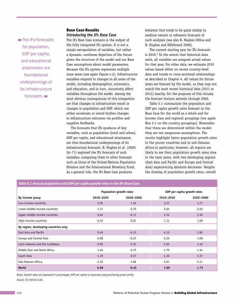
Table 5.1 summarizes the population and GDP per capita growth rates forecast in the Base Case for the world as a whole and for income class and regional groupings (see again Box 2.1 on the country groupings). Remember that these are determined within the model; they are not exogenous assumptions. The results highlight faster population growth rates in the poorer countries and in sub-Saharan Africa in particular; however, all regions are likely to see their population growth rates slow in the later years, with two developing regions (East Asia and Pacific and Europe and Central Asia) experiencing absolute decreases. Despite the slowing of population growth rates, overall
The IFs forecasts for population, GDP per capita,
and educational attainment are
foundational underpinnings of its infrastructure
forecasts.
Table 5.1 Annual population and GDP per capita growth rates in the IFs Base Case
Population growth rates gdP per capita growth rates
By income group 2010–2030 2030–2060 2010–2030 2030–2060
Low-income countries 2.05 1.45 3.23 3.71
Lower-middle-income countries 1.31 0.70 3.64 2.93
Upper-middle-income countries 0.44 -0.11 3.34 2.36
High-income countries 0.35 0.01 1.13 1.09
By region, developing countries only
East Asia and Pacific 0.49 -0.13 4.15 2.83
Europe and Central Asia 0.08 -0.23 2.26 1.08
Latin America and the Caribbean 0.95 0.33 2.05 1.42
Middle East and North Africa 1.46 0.75 1.79 1.34
South Asia 1.19 0.57 4.36 3.37
Sub-Saharan Africa 2.32 1.66 2.61 3.11
World 0.96 0.49 1.89 1.73
Notes: Growth rates are expressed in percentages; GDP per capita is measured using purchasing power parity.
Source: IFs Version 6.61.
Infrastructure Development and Spending in the IFs Base Case 115
population size will continue to increase, and associated with that increase is continued urbanization (not shown in Table 5.1). Globally, the urban share of total population is forecast to grow from just over 50 percent in 2010 to nearly 70 percent in 2060, reflecting increases in all income groups and regions. East Asia and Pacific (which includes China) and South Asia (which includes India) have the fastest growth in GDP per capita, at least in the period out to 2030. With the notable exception of the low-income economies, this growth also slows later in the horizon.
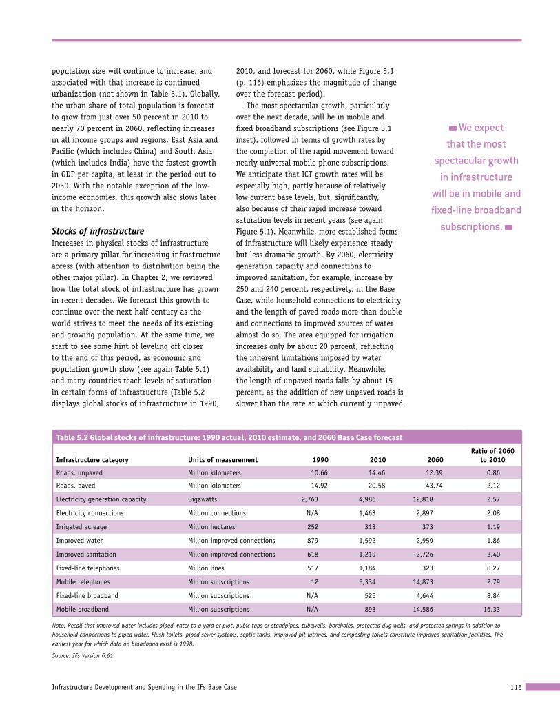
Stocks of infrastructureIncreases in physical stocks of infrastructure are a primary pillar for increasing infrastructure access (with attention to distribution being the other major pillar). In Chapter 2, we reviewed how the total stock of infrastructure has grown in recent decades. We forecast this growth to continue over the next half century as the world strives to meet the needs of its existing and growing population. At the same time, we start to see some hint of leveling off closer to the end of this period, as economic and population growth slow (see again Table 5.1) and many countries reach levels of saturation in certain forms of infrastructure (Table 5.2 displays global stocks of infrastructure in 1990,
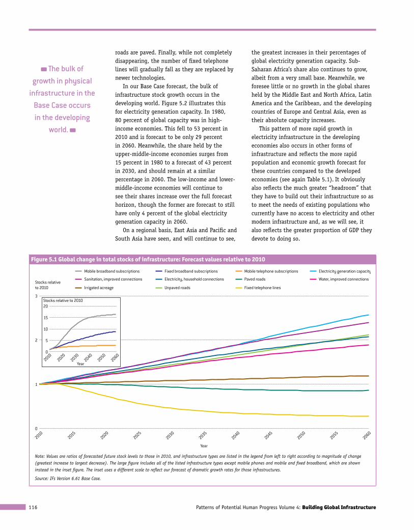
2010, and forecast for 2060, while Figure 5.1 (p. 116) emphasizes the magnitude of change over the forecast period).
The most spectacular growth, particularly over the next decade, will be in mobile and fixed broadband subscriptions (see Figure 5.1 inset), followed in terms of growth rates by the completion of the rapid movement toward nearly universal mobile phone subscriptions. We anticipate that ICT growth rates will be especially high, partly because of relatively low current base levels, but, significantly, also because of their rapid increase toward saturation levels in recent years (see again Figure 5.1). Meanwhile, more established forms of infrastructure will likely experience steady but less dramatic growth. By 2060, electricity generation capacity and connections to improved sanitation, for example, increase by 250 and 240 percent, respectively, in the Base Case, while household connections to electricity and the length of paved roads more than double and connections to improved sources of water almost do so. The area equipped for irrigation increases only by about 20 percent, reflecting the inherent limitations imposed by water availability and land suitability. Meanwhile, the length of unpaved roads falls by about 15 percent, as the addition of new unpaved roads is slower than the rate at which currently unpaved
We expect that the most
spectacular growth in infrastructure
will be in mobile and fixed-line broadband
subscriptions.
Table 5.2 Global stocks of infrastructure: 1990 actual, 2010 estimate, and 2060 Base Case forecast
infrastructure category units of measurement 1990 2010 2060ratio of 2060
to 2010
Roads, unpaved Million kilometers 10.66 14.46 12.39 0.86
Roads, paved Million kilometers 14.92 20.58 43.74 2.12
Electricity generation capacity Gigawatts 2,763 4,986 12,818 2.57
Electricity connections Million connections N/A 1,463 2,897 2.08
Irrigated acreage Million hectares 252 313 373 1.19
Improved water Million improved connections 879 1,592 2,959 1.86
Improved sanitation Million improved connections 618 1,219 2,726 2.40
Fixed-line telephones Million lines 517 1,184 323 0.27
Mobile telephones Million subscriptions 12 5,334 14,873 2.79
Fixed-line broadband Million subscriptions N/A 525 4,644 8.84
Mobile broadband Million subscriptions N/A 893 14,586 16.33
Note: Recall that improved water includes piped water to a yard or plot, pubic taps or standpipes, tubewells, boreholes, protected dug wells, and protected springs in addition to household connections to piped water. Flush toilets, piped sewer systems, septic tanks, improved pit latrines, and composting toilets constitute improved sanitation facilities. The earliest year for which data on broadband exist is 1998.
Source: IFs Version 6.61.
Patterns of Potential Human Progress Volume 4: Building Global Infrastructure116
roads are paved. Finally, while not completely disappearing, the number of fixed telephone lines will gradually fall as they are replaced by newer technologies.
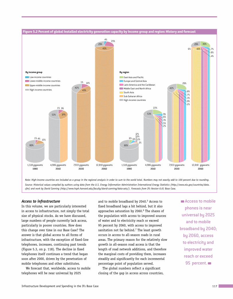
In our Base Case forecast, the bulk of infrastructure stock growth occurs in the developing world. Figure 5.2 illustrates this for electricity generation capacity. In 1980, 80 percent of global capacity was in high-income economies. This fell to 53 percent in 2010 and is forecast to be only 29 percent in 2060. Meanwhile, the share held by the upper-middle-income economies surges from 15 percent in 1980 to a forecast of 43 percent in 2030, and should remain at a similar percentage in 2060. The low-income and lower-middle-income economies will continue to see their shares increase over the full forecast horizon, though the former are forecast to still have only 4 percent of the global electricity generation capacity in 2060.
On a regional basis, East Asia and Pacific and South Asia have seen, and will continue to see,
the greatest increases in their percentages of global electricity generation capacity. Sub-Saharan Africa’s share also continues to grow, albeit from a very small base. Meanwhile, we foresee little or no growth in the global shares held by the Middle East and North Africa, Latin America and the Caribbean, and the developing countries of Europe and Central Asia, even as their absolute capacity increases.
This pattern of more rapid growth in electricity infrastructure in the developing economies also occurs in other forms of infrastructure and reflects the more rapid population and economic growth forecast for these countries compared to the developed economies (see again Table 5.1). It obviously also reflects the much greater “headroom” that they have to build out their infrastructure so as to meet the needs of existing populations who currently have no access to electricity and other modern infrastructure and, as we will see, it also reflects the greater proportion of GDP they devote to doing so.
The bulk of growth in physical
infrastructure in the Base Case occurs in the developing
world.
Figure 5.1 Global change in total stocks of infrastructure: Forecast values relative to 2010
Fixed telephone lines
Fixed broadband subscriptions
Unpaved roads
Paved roads
Mobile broadband subscriptions Mobile telephone subscriptions Electricity generation capacity
Electricity, household connections
Irrigated acreage
Water, improved connectionsSanitation, improved connectionsStocks relative to 2010
3
0
1
2
20102015
20202025
20602050
20402030
20552045
2035
Year
Stocks relative to 201020
15
0
5
10
20102020
20602050
20402030
Year
2
3
Stoc
ks re
lativ
e to
201
0
Mobile broadband subscriptions Fixed broadband subscriptions Mobile telephone subscriptions Sanitation, improved connections Electricity, household connections Paved roads Irrigated acreage Unpaved roads Fixed-line telephone lines
Note: Values are ratios of forecasted future stock levels to those in 2010, and infrastructure types are listed in the legend from left to right according to magnitude of change (greatest increase to largest decrease). The large figure includes all of the listed infrastructure types except mobile phones and mobile and fixed broadband, which are shown instead in the inset figure. The inset uses a different scale to reflect our forecast of dramatic growth rates for those infrastructures.
Source: IFs Version 6.61 Base Case.
Infrastructure Development and Spending in the IFs Base Case 117
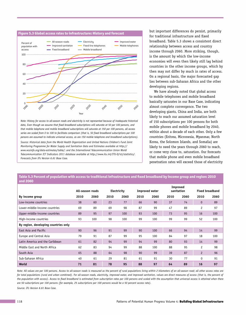
Access to infrastructureIn this volume, we are particularly interested in access to infrastructure, not simply the total size of physical stocks. As we have discussed, large numbers of people currently lack access, particularly in poorer countries. How does this change over time in our Base Case? The answer is that global access to all forms of infrastructure, with the exception of fixed-line telephones, increases, continuing past trends (Figure 5.3, on p. 118). The decline in fixed telephones itself continues a trend that began soon after 2000, driven by the penetration of mobile telephones and other substitutes.
We forecast that, worldwide, access to mobile telephones will be near universal by 2025
and to mobile broadband by 2040.5 Access to fixed broadband lags a bit behind, but it also approaches saturation by 2060.6 The shares of the population with access to improved sources of water and to electricity reach or exceed 95 percent by 2060, with access to improved sanitation not far behind.7 The least growth occurs in access to all-season roads in rural areas. The primary reason for the relatively slow growth in all-season road access is that the length of road network additions, and therefore the marginal costs of providing them, increases steadily and significantly for each incremental percentage point of population served.
The global numbers reflect a significant closing of the gap in access across countries,
Figure 5.2 Percent of global installed electricity generation capacity by income group and region: History and forecast
Low-income countriesLower-middle-income countries
Upper-middle-income countries
1980 2030
By income group
1,518 gigawatts 7,933 gigawatts
1%
1%
1%
14%
9%
43%
37%
15%4%
80%
53%
42%
6%
2%
22%
9%6%
5%2%
53%
29%
8%7%3%
42%
3%
80%
East Asia and PacificEurope and Central AsiaLatin America and the Caribbean
South Asia
Middle East and North Africa
Sub-Saharan AfricaHigh-income countries
By region
206012,818 gigawatts
4%23%
43%
29%
2060
30%
7%8%4%
16%6%
29%
12,818 gigawatts2010
4,986 gigawatts
High-income countries
20307,933 gigawatts
20104,986 gigawatts
19801,518 gigawatts
2%2%
2%6%
9%2%
Note: High-income countries are included as a group in the regional analysis in order to sum to the world total. Numbers may not exactly add to 100 percent due to rounding.
Source: Historical values compiled by authors using data from the U.S. Energy Information Administration International Energy Statistics (http://www.eia.gov/countries/data.cfm) and work by David Canning (http://www.hsph.harvard.edu/faculty/david-canning/data-sets/). Forecasts from IFs Version 6.61 Base Case.
Access to mobile phones is near
universal by 2025 and to mobile
broadband by 2040; by 2060, access to electricity and improved water reach or exceed 95 percent.
Patterns of Potential Human Progress Volume 4: Building Global Infrastructure118
but important differences do persist, primarily for traditional infrastructure and fixed broadband. Table 5.3 shows a consistent direct relationship between access and country income through 2060. More striking, though, is the amount by which the low-income economies will even then likely still lag behind countries in the other income groups, which by then may not differ by much in rates of access. On a regional basis, the major forecasted gap lies between sub-Saharan Africa and the other developing regions.
We have already noted that global access to mobile telephones and mobile broadband basically saturates in our Base Case, indicating almost complete convergence. The two developing giants, China and India, are both likely to reach our assumed saturation level of 150 subscriptions per 100 persons for both mobile phones and mobile broadband by 2040, within about a decade of each other. Only a few countries (Eritrea, Micronesia, Myanmar, North Korea, the Solomon Islands, and Somalia) are likely to need the years through 2060 to reach, or come very close to, saturation. Our forecasts that mobile phone and even mobile broadband penetration rates will exceed those of electricity
Table 5.3 Percent of population with access to traditional infrastructure and fixed broadband by income group and region: 2010 and 2060
all-season roads electricity improved waterimproved sanitation fixed broadband
By income group 2010 2060 2010 2060 2010 2060 2010 2060 2010 2060
Low-income countries 38 60 23 77 66 90 37 74 0 89
Lower-middle-income countries 69 89 69 98 87 99 47 89 2 97
Upper-middle-income countries 89 95 97 100 93 100 73 95 16 100
High-income countries 93 100 98 100 99 100 99 99 52 100
By region, developing countries only
East Asia and Pacific 90 96 91 99 90 100 66 94 14 99
Europe and Central Asia 79 91 87 99 95 100 84 97 18 100
Latin America and the Caribbean 61 82 94 99 94 99 80 93 14 99
Middle East and North Africa 62 83 94 99 88 100 88 95 2 98
South Asia 65 88 64 98 90 99 39 87 2 96
Sub-Saharan Africa 40 61 29 81 61 91 30 77 0 91
World 71 81 78 95 88 97 64 89 16 97
Note: All values are per 100 persons. Access to all-season roads is measured as the percent of rural populations living within 2 kilometers of an all-season road; all other access rates are for total populations (rural and urban combined). For all-season roads, electricity, improved water, and improved sanitation, values are direct measures of access (that is, the percent of the population with access). Access to fixed broadband is estimated from subscription rates per 100 persons and scaled with the assumption that universal access is attained when there are 50 subscriptions per 100 persons (for example, 25 subscriptions per 100 persons would be a 50 percent access rate).
Source: IFs Version 6.61 Base Case.
Figure 5.3 Global access rates to infrastructure: History and forecast
Improved sanitation Fixed-line telephonesFixed broadband
Mobile telephonesAll-season roads Electricity Improved water
Mobile broadband
Percent of population with access
100
0
20
40
60
80
19902060
20502040
20102000
20302020
Year
Note: History for access to all-season roads and electricity is not represented because of inadequate historical data, Even though we assume that fixed broadband subscriptions will saturate at 50 per 100 persons, and that mobile telephone and mobile broadband subscriptions will saturate at 150 per 100 persons, all access series are scaled from 0 to 100 to facilitate comparison (that is, 50 fixed broadband subscriptions per 100 persons are assumed to indicate universal access, as are 150 mobile telephone and broadband subscriptions).
Source: Historical data from the World Health Organization and United Nations Children’s Fund Joint Monitoring Programme for Water Supply and Sanitation Data and Estimates available at http://www.wssinfo.org/data-estimates/table/; and the International Telecommunication Union World Telecommunication ICT Indicators 2011 database available at http://www.itu.int/ITU-D/ict/statistics/. Forecasts from IFs Version 6.61 Base Case.
Infrastructure Development and Spending in the IFs Base Case 119
in a very short time, and continue to outstrip them for much of our forecast horizon, may be surprising—after all, it takes electricity to charge the phones. The fact is, however, that recent data suggest that many countries—including Chad, Kenya, Liberia, Rwanda, Sierra Leone, Uganda, and Vanuatu—already have higher access rates for mobile telephones than for electricity. In such countries, where the mobile phone penetration rate can be several times that of electricity, mechanisms such as communal charging stations and electricity access from relatives and friends can provide battery recharging capability.
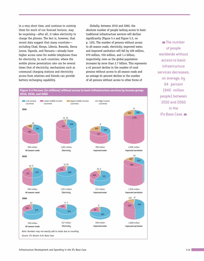
Globally, between 2010 and 2060, the absolute number of people lacking access to basic traditional infrastructure services will decline significantly (Figure 5.4 and Figure 5.5, on p. 120). The number of persons without access to all-season roads, electricity, improved water, and improved sanitation will fall by 400 million, 970 million, 550 million, and 1.4 billion, respectively, even as the global population increases by more than 2.7 billion. This represents a 42 percent decline in the number of rural persons without access to all-season roads and an average 64 percent decline in the number of all persons without access to other forms of
The number of people
worldwide without access to basic infrastructure
services decreases, on average, by
64 percent (840 million
people) between 2010 and 2060
in the IFs Base Case.
Figure 5.4 Persons (in millions) without access to basic infrastructure services by income group: 2010, 2030, and 2060
Low-incomecountries
Lower-middle-incomecountries
Upper-middle-incomecountries
High-incomecountries
2010
Electricity1,491 million
75
628
21
767
Electricity1,011 million
20
271689
31
Electricity517 million
6
431
4
77
Improved sanitation2,482 million
11
1,291
518662
Improved sanitation1,956 million
24
982
622327
Improved sanitation1,068 million
17
420 499
132
All-season roads964 million
16
367120
461
All-season roads854 million
2030
6
371 425
52
All-season roads559 million
2060
373164
22
Improved water789 million
8
317
280184
Improved water531 million
35
321
6
168
Improved water240 million
9
183
48
Note: Numbers may not exactly add to totals due to rounding.
Source: IFs Version 6.61 Base Case.
Patterns of Potential Human Progress Volume 4: Building Global Infrastructure120
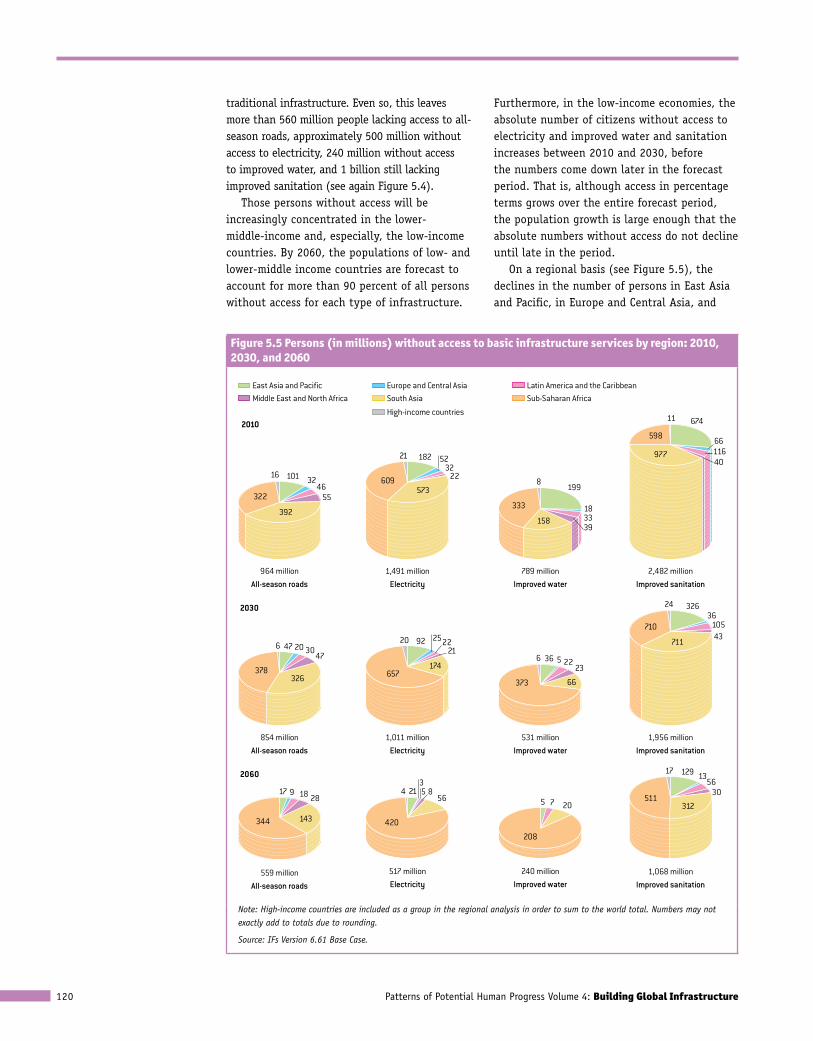
traditional infrastructure. Even so, this leaves more than 560 million people lacking access to all-season roads, approximately 500 million without access to electricity, 240 million without access to improved water, and 1 billion still lacking improved sanitation (see again Figure 5.4).
Those persons without access will be increasingly concentrated in the lower-middle-income and, especially, the low-income countries. By 2060, the populations of low- and lower-middle income countries are forecast to account for more than 90 percent of all persons without access for each type of infrastructure.
Furthermore, in the low-income economies, the absolute number of citizens without access to electricity and improved water and sanitation increases between 2010 and 2030, before the numbers come down later in the forecast period. That is, although access in percentage terms grows over the entire forecast period, the population growth is large enough that the absolute numbers without access do not decline until late in the period.
On a regional basis (see Figure 5.5), the declines in the number of persons in East Asia and Pacific, in Europe and Central Asia, and
Figure 5.5 Persons (in millions) without access to basic infrastructure services by region: 2010, 2030, and 2060
East Asia and Pacific Europe and Central Asia Latin America and the CaribbeanMiddle East and North Africa South Asia Sub-Saharan Africa
High-income countries2010
55
All-season roads964 million
101
All-season roads854 million
2030
All-season roads559 million
2060
3246
392
322
16
47 20 3047
326378
6
17 9 18 28
143344
Improved sanitation2,482 million
Improved sanitation1,956 million
Improved sanitation1,068 million
674
6611640
977
598
11
32636
10543
711
710
24
1713
5630
312511
129
3222
Electricity1,491 million
Electricity1,011 million
Electricity517 million
182 52
573609
21
92 252221
174657
20
213
856
420
4 5
Improved water
Improved water789 million
Improved water531 million
240 million
199
183339
158
333
8
36 5 2223
66373
6
5 7 20
208
Note: High-income countries are included as a group in the regional analysis in order to sum to the world total. Numbers may not exactly add to totals due to rounding.
Source: IFs Version 6.61 Base Case.
Infrastructure Development and Spending in the IFs Base Case 121
in South Asia without access to electricity, improved water, and improved sanitation are approximately 80 to 90 percent between 2010 and 2060. That still leaves a significant number of people, such as 129 million in East Asia and Pacific and 312 million in South Asia, without access to improved sanitation, due to the large populations in these regions. Latin America and the Caribbean and the Middle East and North Africa perform as well in reducing the numbers of persons without access to electricity and improved water, but see lesser declines, about 25 to 50 percent respectively, for access to improved sanitation. Meanwhile, the decreases in those without access in sub-Saharan Africa are only about 15 to 40 percent, depending on the type of infrastructure. As a result, by 2060 we anticipate that large majorities of those who still lack access to traditional infrastructure will live in sub-Saharan Africa.
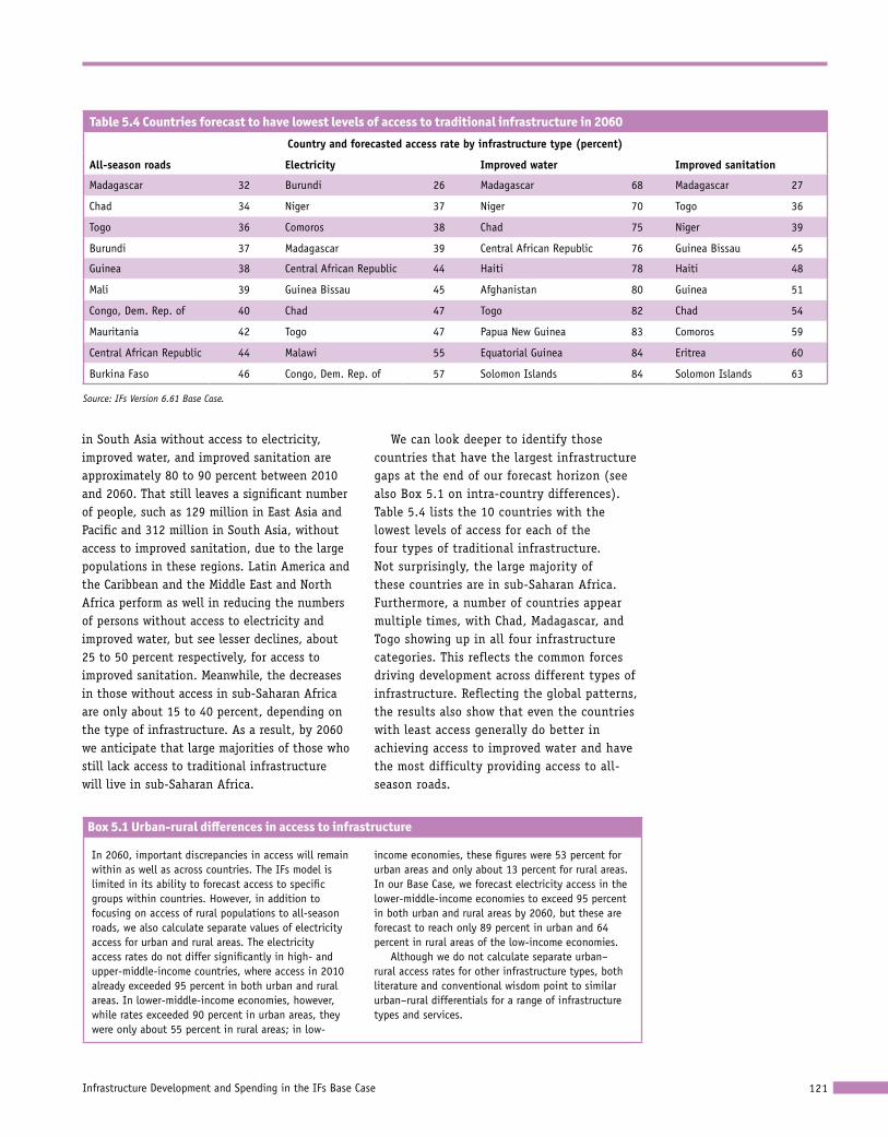
We can look deeper to identify those countries that have the largest infrastructure gaps at the end of our forecast horizon (see also Box 5.1 on intra-country differences). Table 5.4 lists the 10 countries with the lowest levels of access for each of the four types of traditional infrastructure. Not surprisingly, the large majority of these countries are in sub-Saharan Africa. Furthermore, a number of countries appear multiple times, with Chad, Madagascar, and Togo showing up in all four infrastructure categories. This reflects the common forces driving development across different types of infrastructure. Reflecting the global patterns, the results also show that even the countries with least access generally do better in achieving access to improved water and have the most difficulty providing access to all-season roads.
Table 5.4 Countries forecast to have lowest levels of access to traditional infrastructure in 2060
country and forecasted access rate by infrastructure type (percent)
all-season roads electricity improved water improved sanitation
Madagascar 32 Burundi 26 Madagascar 68 Madagascar 27
Chad 34 Niger 37 Niger 70 Togo 36
Togo 36 Comoros 38 Chad 75 Niger 39
Burundi 37 Madagascar 39 Central African Republic 76 Guinea Bissau 45
Guinea 38 Central African Republic 44 Haiti 78 Haiti 48
Mali 39 Guinea Bissau 45 Afghanistan 80 Guinea 51
Congo, Dem. Rep. of 40 Chad 47 Togo 82 Chad 54
Mauritania 42 Togo 47 Papua New Guinea 83 Comoros 59
Central African Republic 44 Malawi 55 Equatorial Guinea 84 Eritrea 60
Burkina Faso 46 Congo, Dem. Rep. of 57 Solomon Islands 84 Solomon Islands 63
Source: IFs Version 6.61 Base Case.
Box 5.1 Urban-rural differences in access to infrastructure
In 2060, important discrepancies in access will remain within as well as across countries. The IFs model is limited in its ability to forecast access to specific groups within countries. However, in addition to focusing on access of rural populations to all-season roads, we also calculate separate values of electricity access for urban and rural areas. The electricity access rates do not differ significantly in high- and upper-middle-income countries, where access in 2010 already exceeded 95 percent in both urban and rural areas. In lower-middle-income economies, however, while rates exceeded 90 percent in urban areas, they were only about 55 percent in rural areas; in low-
income economies, these figures were 53 percent for urban areas and only about 13 percent for rural areas. In our Base Case, we forecast electricity access in the lower-middle-income economies to exceed 95 percent in both urban and rural areas by 2060, but these are forecast to reach only 89 percent in urban and 64 percent in rural areas of the low-income economies.
Although we do not calculate separate urban–rural access rates for other infrastructure types, both literature and conventional wisdom point to similar urban–rural differentials for a range of infrastructure types and services.
Patterns of Potential Human Progress Volume 4: Building Global Infrastructure122
Spending on infrastructureInfrastructure, and access to it, have high costs for countries. Box 5.2 summarizes how we estimate infrastructure spending (see again Chapter 4 for a more complete description). Building on our discussion of the ongoing transitions in the physical types and patterns of global infrastructure, forecasting of spending allows us to (1) consider the likely evolution of total infrastructure spending globally; (2) explore the changing size of infrastructure spending in global and national economies; and (3) drill down into infrastructure-specific spending.
Global spending totals In our Base Case, global infrastructure spending over the next 50 years is over $171 trillion in year 2000 constant dollars. Our value of $46 trillion from 2010–2030 is very much in line
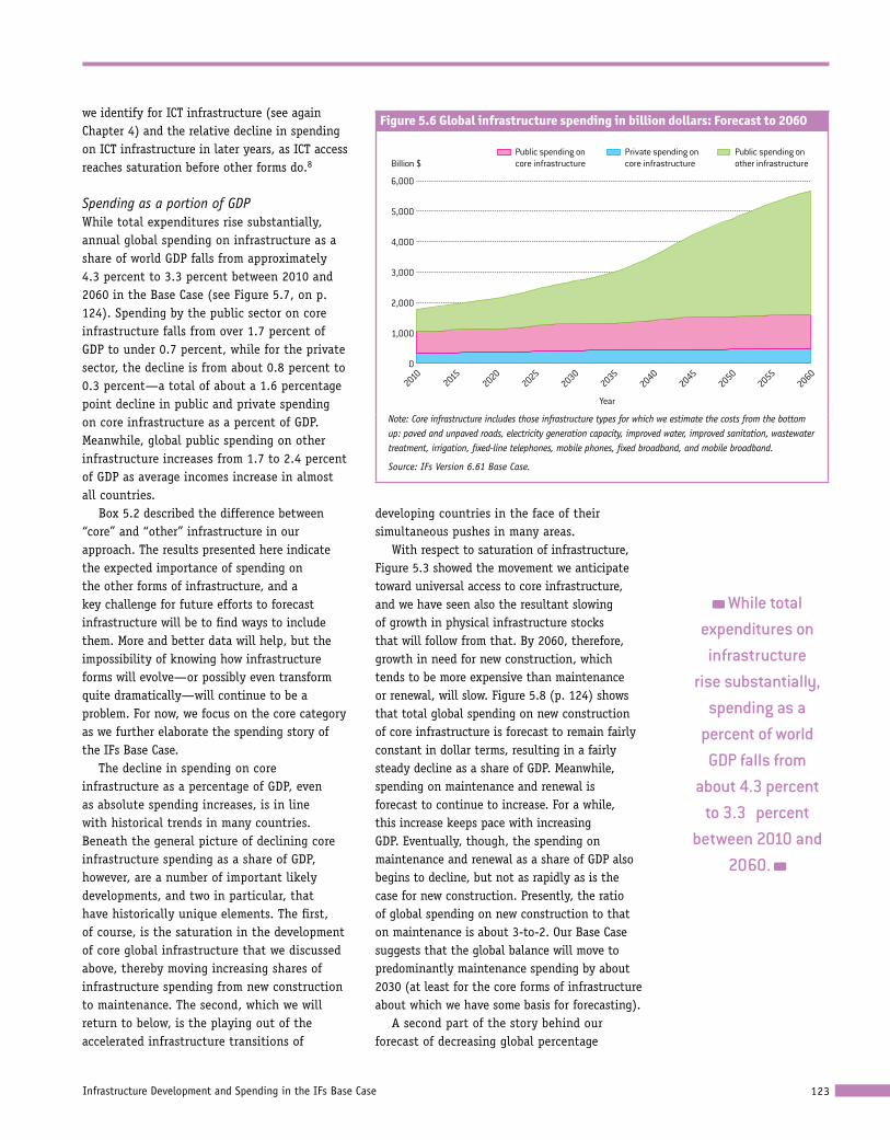
with an earlier Organisation for Economic Co-operation and Development (OECD) estimate of $53 trillion from 2000–2030 (Stevens, Schieb, and Andrieu 2006: 29). Annual spending gradually increases from $1.8 trillion in 2010 to $5.6 trillion in 2060 (see Figure 5.6). The bulk of this increase is due to increased public spending on “other” infrastructure (see again Box 5.2), which grows from just over $700 billion in 2010 to $4 trillion in 2060, a more than 500 percent increase. Meanwhile, the annual public and private spending on “core” infrastructure, that is, those infrastructure types we model explicitly, only increases by 60 and 40 percent, respectively, over this period. The global ratio of public to private spending on core infrastructure starts at a bit over 2-to-1, rising to about 2.40-to-1 by 2060. This gradual shift to a larger public contribution is due to a combination of the greater current private share
In the Base Case, global
infrastructure spending over the next 50 years is
over 171 trillion in 2000 dollars.
Box 5.2 Estimating infrastructure spending in IFs
In Chapter 2, we described the difficulty in finding comprehensive and comparable data on infrastructure spending, and in Chapter 4 we explained our approach to estimating spending on infrastructure in our base year (2010), as well as in our forecast years. In brief, we estimate spending for two broad categories of infrastructure: those types of infrastructure explicitly identified in our modeling, which we refer to as “core” infrastructure,* and “other” infrastructure, for example, railroads, airports, and seaports. Other infrastructure would also include new not-yet-known forms with potentially transformative importance, including assisting in shifts toward sustainable infrastructures for the future. Spending for the core category is estimated from the bottom-up, based on levels of physical infrastructure and assumptions about unit costs and lifetimes for each type of infrastructure. We calculate spending on new construction and on maintenance separately and use infrastructure-specific share parameters to divide the spending between public and private sources. For spending in the other infrastructure category, we consider only that portion provided by the public sector (which we assume is almost all of it) and estimate this as a simple function of GDP per capita.
Some key assumptions of our approach are:
■■ The infrastructure-specific unit costs, lifetimes, and public shares do not vary across country, time, income level, or existing levels of infrastructure.
■■ For the most part** the spending is attributed to the year that the infrastructure is completed and “comes online”—that is, we do not try to spread out the spending on new construction over the life of individual projects, which is often many years.
■■ Only public sector spending is used when calculating the balance between spending demands and available funds.
■■ Any shortfalls in public spending are matched by proportionate reductions in private sector spending except for ICT, which remains unchanged.
The spending values for the starting year of forecasts (2010) are estimated from historical data on growth in the amount of physical infrastructure. While these are not forced to match the few existing estimates of actual spending, our analysis showed that the numbers were roughly comparable.
Finally, all spending figures in dollars are presented in year 2000 constant dollars based on market exchange rates. Spending as a percentage of GDP is determined by the spending in dollars divided by GDP based on market exchange rates.
* Core infrastructure includes paved and unpaved roads, electricity generation capacity, improved water, improved sanitation, wastewater treatment, irrigation, fixed-line telephones, mobile phones, fixed broadband, and mobile broadband.
** When exceptional spending surges are forecast, we spread their translation into additional capacity across several years (see Chapter 4).
Infrastructure Development and Spending in the IFs Base Case 123
we identify for ICT infrastructure (see again Chapter 4) and the relative decline in spending on ICT infrastructure in later years, as ICT access reaches saturation before other forms do.8
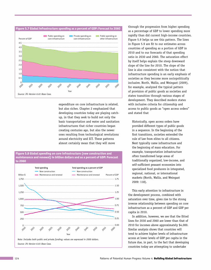
Spending as a portion of GDP While total expenditures rise substantially, annual global spending on infrastructure as a share of world GDP falls from approximately 4.3 percent to 3.3 percent between 2010 and 2060 in the Base Case (see Figure 5.7, on p. 124). Spending by the public sector on core infrastructure falls from over 1.7 percent of GDP to under 0.7 percent, while for the private sector, the decline is from about 0.8 percent to 0.3 percent—a total of about a 1.6 percentage point decline in public and private spending on core infrastructure as a percent of GDP. Meanwhile, global public spending on other infrastructure increases from 1.7 to 2.4 percent of GDP as average incomes increase in almost all countries.
Box 5.2 described the difference between “core” and “other” infrastructure in our approach. The results presented here indicate the expected importance of spending on the other forms of infrastructure, and a key challenge for future efforts to forecast infrastructure will be to find ways to include them. More and better data will help, but the impossibility of knowing how infrastructure forms will evolve—or possibly even transform quite dramatically—will continue to be a problem. For now, we focus on the core category as we further elaborate the spending story of the IFs Base Case.
The decline in spending on core infrastructure as a percentage of GDP, even as absolute spending increases, is in line with historical trends in many countries. Beneath the general picture of declining core infrastructure spending as a share of GDP, however, are a number of important likely developments, and two in particular, that have historically unique elements. The first, of course, is the saturation in the development of core global infrastructure that we discussed above, thereby moving increasing shares of infrastructure spending from new construction to maintenance. The second, which we will return to below, is the playing out of the accelerated infrastructure transitions of
developing countries in the face of their simultaneous pushes in many areas.
With respect to saturation of infrastructure, Figure 5.3 showed the movement we anticipate toward universal access to core infrastructure, and we have seen also the resultant slowing of growth in physical infrastructure stocks that will follow from that. By 2060, therefore, growth in need for new construction, which tends to be more expensive than maintenance or renewal, will slow. Figure 5.8 (p. 124) shows that total global spending on new construction of core infrastructure is forecast to remain fairly constant in dollar terms, resulting in a fairly steady decline as a share of GDP. Meanwhile, spending on maintenance and renewal is forecast to continue to increase. For a while, this increase keeps pace with increasing GDP. Eventually, though, the spending on maintenance and renewal as a share of GDP also begins to decline, but not as rapidly as is the case for new construction. Presently, the ratio of global spending on new construction to that on maintenance is about 3-to-2. Our Base Case suggests that the global balance will move to predominantly maintenance spending by about 2030 (at least for the core forms of infrastructure about which we have some basis for forecasting).
A second part of the story behind our forecast of decreasing global percentage
Figure 5.6 Global infrastructure spending in billion dollars: Forecast to 2060
Private spending on core infrastructure
Public spending on core infrastructure
Public spending on other infrastructureBillion $
6,000
0
1,000
2,000
3,000
4,000
5,000
20102060
20402030
20502055
20452035
20202025
2015
Year
Note: Core infrastructure includes those infrastructure types for which we estimate the costs from the bottom up: paved and unpaved roads, electricity generation capacity, improved water, improved sanitation, wastewater treatment, irrigation, fixed-line telephones, mobile phones, fixed broadband, and mobile broadband.
Source: IFs Version 6.61 Base Case.
While total expenditures on
infrastructure rise substantially,
spending as a percent of world
GDP falls from about 4.3 percent
to 3.3 percent between 2010 and
2060.
Patterns of Potential Human Progress Volume 4: Building Global Infrastructure124
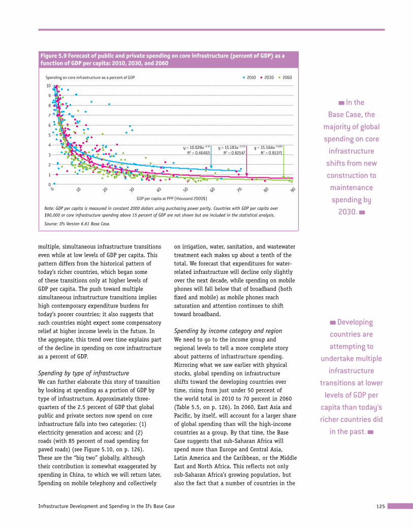
expenditure on core infrastructure is related, but also richer. Chapter 2 emphasized that developing countries today are playing catch-up, in that they seek to build not only the basic transportation and water and sanitation infrastructures that richer countries began creating centuries ago, but also the newer ones resulting from technological revolutions around electricity and ICT. These patterns almost certainly mean that they will move
through the progression from higher spending as a percentage of GDP to lower spending more rapidly than did current high-income countries. Figure 5.9 helps us see this pattern. The lines in Figure 5.9 are fit to our estimates across countries of spending as a portion of GDP in 2010 and to our forecasts of that spending ratio in 2030 and 2060. The saturation effect by itself helps explain the steep downward slope of the line for 2010. The slope of the line is also consistent with the notion that infrastructure spending is an early emphasis of societies as they become more sociopolitically inclusive. North, Wallis, and Weingast (2009), for example, analyzed the typical pattern of provision of public goods as societies and states transition through various stages of development. They described modern states with inclusive criteria for citizenship and access to public goods as “open access orders” and stated that
Historically, open access orders have provided different types of public goods in a sequence. In the beginning of the first transitions, societies extended the rule of law from elites to all citizens. Next typically came infrastructure and the beginning of mass education. For example, transportation infrastructure often transformed large areas of traditionally organized, low-income, and self-sufficient peasant economies into specialized food producers in integrated, regional, national, or international markets (North, Wallis, and Weingast 2009: 118).
This early attention to infrastructure in the development process, combined with saturation over time, gives rise to the strong inverse relationship between spending on core infrastructure as a percent of GDP and GDP per capita in 2010.
In addition, however, we see that the fitted lines for 2030 and 2060 are lower than that of 2010 for incomes above approximately $4,000. Similar analysis shows that countries will tend to achieve higher levels of infrastructure access at lower levels of GDP per capita in the future due, in part, to the fact that developing countries today are attempting to undertake
Figure 5.7 Global infrastructure spending as a percent of GDP: Forecast to 2060
Private spending on core infrastructure
Public spending on core infrastructure
Public spending on other infrastructurePercent of GDP
4.5
0
0.5
1.0
1.5
2.0
2.5
3.5
3.0
4.0
20102060
20402030
20502055
20452035
20202025
2015
YearSource: IFs Version 6.61 Base Case.
Figure 5.8 Global spending on core infrastructure (new construction and maintenance and renewal) in billion dollars and as a percent of GDP: Forecast to 2060
Total spending Total spending as a percent of GDP
New construction Maintenance and renewal
New construction Maintenance and renewalBillion $ Percent of GDP
1,750 1.75
1.50
1.25
1.00
0.75
0.50
0.25
0.000
500
250
750
1,000
1,250
1,500
20102060
20502055
20402030
20452035
20202025
2015
Year
Note: Includes both public and private funding; values are expressed in 2000 dollars.
Source: IFs Version 6.61 Base Case.
Infrastructure Development and Spending in the IFs Base Case 125
multiple, simultaneous infrastructure transitions even while at low levels of GDP per capita. This pattern differs from the historical pattern of today’s richer countries, which began some of these transitions only at higher levels of GDP per capita. The push toward multiple simultaneous infrastructure transitions implies high contemporary expenditure burdens for today’s poorer countries; it also suggests that such countries might expect some compensatory relief at higher income levels in the future. In the aggregate, this trend over time explains part of the decline in spending on core infrastructure as a percent of GDP.
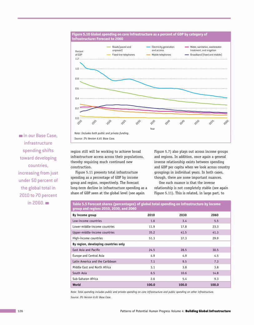
Spending by type of infrastructureWe can further elaborate this story of transition by looking at spending as a portion of GDP by type of infrastructure. Approximately three-quarters of the 2.5 percent of GDP that global public and private sectors now spend on core infrastructure falls into two categories: (1) electricity generation and access; and (2) roads (with 85 percent of road spending for paved roads) (see Figure 5.10, on p. 126). These are the “big two” globally, although their contribution is somewhat exaggerated by spending in China, to which we will return later. Spending on mobile telephony and collectively
on irrigation, water, sanitation, and wastewater treatment each makes up about a tenth of the total. We forecast that expenditures for water-related infrastructure will decline only slightly over the next decade, while spending on mobile phones will fall below that of broadband (both fixed and mobile) as mobile phones reach saturation and attention continues to shift toward broadband.
Spending by income category and regionWe need to go to the income group and regional levels to tell a more complete story about patterns of infrastructure spending. Mirroring what we saw earlier with physical stocks, global spending on infrastructure shifts toward the developing countries over time, rising from just under 50 percent of the world total in 2010 to 70 percent in 2060 (Table 5.5, on p. 126). In 2060, East Asia and Pacific, by itself, will account for a larger share of global spending than will the high-income countries as a group. By that time, the Base Case suggests that sub-Saharan Africa will spend more than Europe and Central Asia, Latin America and the Caribbean, or the Middle East and North Africa. This reflects not only sub-Saharan Africa’s growing population, but also the fact that a number of countries in the
Figure 5.9 Forecast of public and private spending on core infrastructure (percent of GDP) as a function of GDP per capita: 2010, 2030, and 2060
2010 2030 2060Spending on core infrastructure as a percent of GDP
10
0
2
1
3
4
5
6
9
7
8
0 906040 80705020 3010
GDP per capita at PPP (thousand 2000$)
y = 10.028x–0.47
R2 = 0.46465y = 15.183x–0.713
R2 = 0.82147y = 15.564x–0.802
R2 = 0.81371
Note: GDP per capita is measured in constant 2000 dollars using purchasing power parity. Countries with GDP per capita over $90,000 or core infrastructure spending above 15 percent of GDP are not shown but are included in the statistical analysis.
Source: IFs Version 6.61 Base Case.
In the Base Case, the
majority of global spending on core
infrastructure shifts from new construction to
maintenance spending by
2030.
Developing countries are attempting to
undertake multiple infrastructure
transitions at lower levels of GDP per
capita than today’s richer countries did
in the past.
Patterns of Potential Human Progress Volume 4: Building Global Infrastructure126
region still will be working to achieve broad infrastructure access across their populations, thereby requiring much continued new construction.
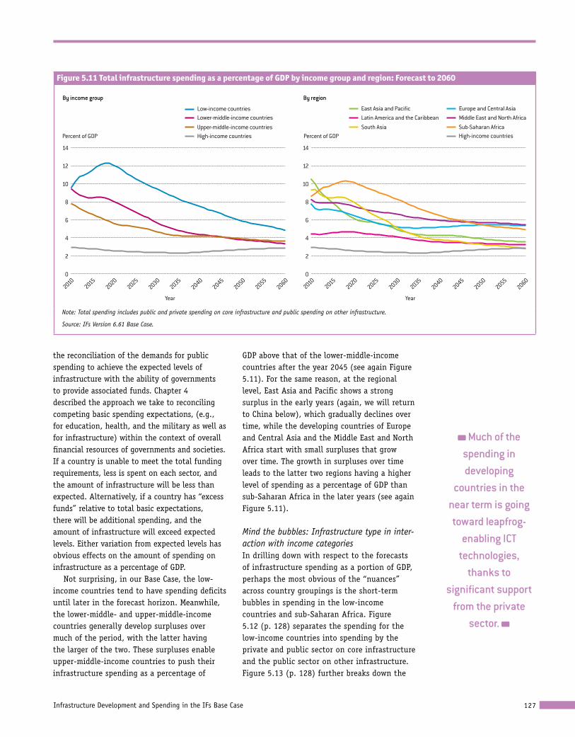
Figure 5.11 presents total infrastructure spending as a percentage of GDP by income group and region, respectively. The forecast long-term decline in infrastructure spending as a share of GDP seen at the global level (see again
Figure 5.7) also plays out across income groups and regions. In addition, once again a general inverse relationship exists between spending and GDP per capita when we look across country groupings in individual years. In both cases, though, there are some important nuances.
One such nuance is that the inverse relationship is not completely stable (see again Figure 5.11). This is related, in large part, to
In our Base Case, infrastructure
spending shifts toward developing
countries, increasing from just under 50 percent of
the global total in 2010 to 70 percent
in 2060.
Figure 5.10 Global spending on core infrastructure as a percent of GDP by category of infrastructure: Forecast to 2060
Fixed-line telephones Broadband (�xed and mobile)Mobile telephones
Roads(paved and unpaved)
Electricity generation and access
Water, sanitation, wastewater treatment, and irrigationPercent
of GDP1.2
0.0
0.4
0.2
0.6
0.8
1.0
20102015
20202025
20602050
20402030
20552045
2035
Year
Note: Includes both public and private funding.
Source: IFs Version 6.61 Base Case.
Table 5.5 Forecast shares (percentages) of global total spending on infrastructure by income group and region: 2010, 2030, and 2060
By income group 2010 2030 2060
Low-income countries 1.6 3.4 5.5
Lower-middle-income countries 11.9 17.8 23.3
Upper-middle-income countries 35.2 41.5 41.3
High-income countries 51.3 37.3 29.9
By region, developing countries only
East Asia and Pacific 24.5 28.5 30.5
Europe and Central Asia 4.9 4.9 4.5
Latin America and the Caribbean 7.1 9.5 7.3
Middle East and North Africa 3.1 3.8 3.8
South Asia 6.5 10.6 14.8
Sub-Saharan Africa 2.6 5.4 9.3
World 100.0 100.0 100.0
Note: Total spending includes public and private spending on core infrastructure and public spending on other infrastructure.
Source: IFs Version 6.61 Base Case.
Infrastructure Development and Spending in the IFs Base Case 127
Much of the spending in developing
countries in the near term is going toward leapfrog-
enabling ICT technologies,
thanks to significant support
from the private sector.
the reconciliation of the demands for public spending to achieve the expected levels of infrastructure with the ability of governments to provide associated funds. Chapter 4 described the approach we take to reconciling competing basic spending expectations, (e.g., for education, health, and the military as well as for infrastructure) within the context of overall financial resources of governments and societies. If a country is unable to meet the total funding requirements, less is spent on each sector, and the amount of infrastructure will be less than expected. Alternatively, if a country has “excess funds” relative to total basic expectations, there will be additional spending, and the amount of infrastructure will exceed expected levels. Either variation from expected levels has obvious effects on the amount of spending on infrastructure as a percentage of GDP.
Not surprising, in our Base Case, the low-income countries tend to have spending deficits until later in the forecast horizon. Meanwhile, the lower-middle- and upper-middle-income countries generally develop surpluses over much of the period, with the latter having the larger of the two. These surpluses enable upper-middle-income countries to push their infrastructure spending as a percentage of
GDP above that of the lower-middle-income countries after the year 2045 (see again Figure 5.11). For the same reason, at the regional level, East Asia and Pacific shows a strong surplus in the early years (again, we will return to China below), which gradually declines over time, while the developing countries of Europe and Central Asia and the Middle East and North Africa start with small surpluses that grow over time. The growth in surpluses over time leads to the latter two regions having a higher level of spending as a percentage of GDP than sub-Saharan Africa in the later years (see again Figure 5.11).
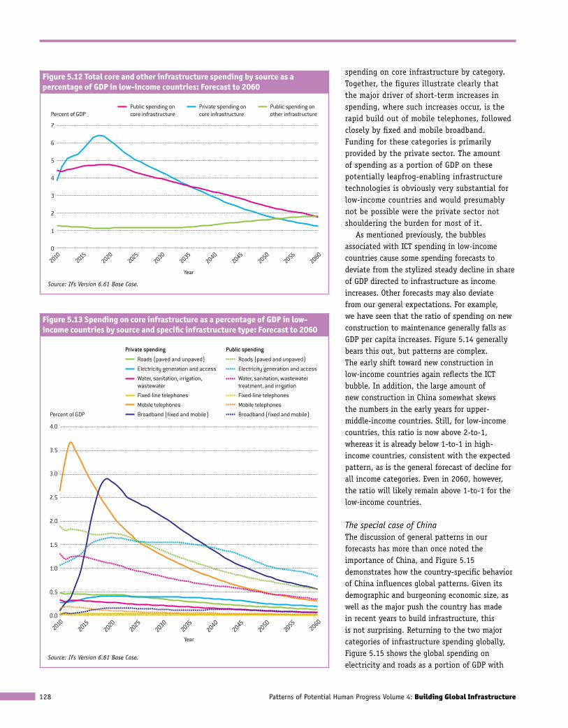
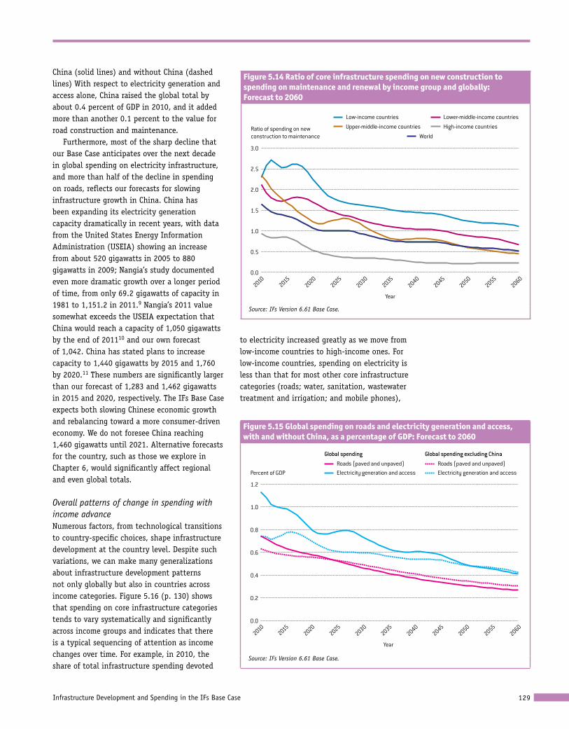
Mind the bubbles: Infrastructure type in inter-action with income categoriesIn drilling down with respect to the forecasts of infrastructure spending as a portion of GDP, perhaps the most obvious of the “nuances” across country groupings is the short-term bubbles in spending in the low-income countries and sub-Saharan Africa. Figure 5.12 (p. 128) separates the spending for the low-income countries into spending by the private and public sector on core infrastructure and the public sector on other infrastructure. Figure 5.13 (p. 128) further breaks down the
Figure 5.11 Total infrastructure spending as a percentage of GDP by income group and region: Forecast to 2060
Percent of GDP Percent of GDP
14
0
2
4
6
8
10
12
20102040
20302060
20452050
20552035
20202025
2015
Year
14
0
2
4
6
8
10
12
20102040
20302060
20452050
20552035
20202025
2015
Year
East Asia and Paci�c Europe and Central AsiaLatin America and the CaribbeanSouth Asia Sub-Saharan Africa
High-income countries
Middle East and North Africa Low-income countries
By income group By region
Lower-middle-income countries
Upper-middle-income countriesHigh-income countries
Note: Total spending includes public and private spending on core infrastructure and public spending on other infrastructure.
Source: IFs Version 6.61 Base Case.
Patterns of Potential Human Progress Volume 4: Building Global Infrastructure128
spending on core infrastructure by category. Together, the figures illustrate clearly that the major driver of short-term increases in spending, where such increases occur, is the rapid build out of mobile telephones, followed closely by fixed and mobile broadband. Funding for these categories is primarily provided by the private sector. The amount of spending as a portion of GDP on these potentially leapfrog-enabling infrastructure technologies is obviously very substantial for low-income countries and would presumably not be possible were the private sector not shouldering the burden for most of it.
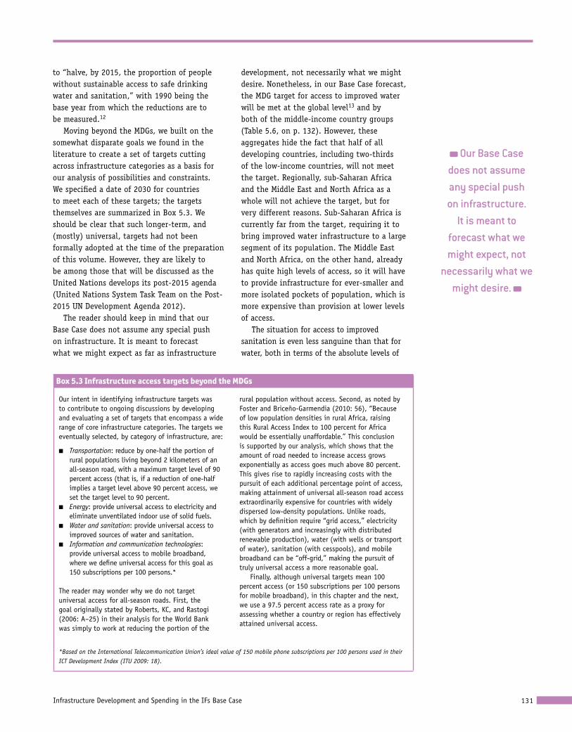
As mentioned previously, the bubbles associated with ICT spending in low-income countries cause some spending forecasts to deviate from the stylized steady decline in share of GDP directed to infrastructure as income increases. Other forecasts may also deviate from our general expectations. For example, we have seen that the ratio of spending on new construction to maintenance generally falls as GDP per capita increases. Figure 5.14 generally bears this out, but patterns are complex. The early shift toward new construction in low-income countries again reflects the ICT bubble. In addition, the large amount of new construction in China somewhat skews the numbers in the early years for upper-middle-income countries. Still, for low-income countries, this ratio is now above 2-to-1, whereas it is already below 1-to-1 in high-income countries, consistent with the expected pattern, as is the general forecast of decline for all income categories. Even in 2060, however, the ratio will likely remain above 1-to-1 for the low-income countries.
The special case of China The discussion of general patterns in our forecasts has more than once noted the importance of China, and Figure 5.15 demonstrates how the country-specific behavior of China influences global patterns. Given its demographic and burgeoning economic size, as well as the major push the country has made in recent years to build infrastructure, this is not surprising. Returning to the two major categories of infrastructure spending globally, Figure 5.15 shows the global spending on electricity and roads as a portion of GDP with
Figure 5.12 Total core and other infrastructure spending by source as a percentage of GDP in low-income countries: Forecast to 2060
Private spending on core infrastructure
Public spending on core infrastructure
Public spending on other infrastructurePercent of GDP
7
0
1
2
3
4
5
6
20102060
20402030
20502055
20452035
20202025
2015
Year
Source: IFs Version 6.61 Base Case.
Figure 5.13 Spending on core infrastructure as a percentage of GDP in low-income countries by source and specific infrastructure type: Forecast to 2060
Private spending
Roads (paved and unpaved)
Electricity generation and access
Water, sanitation, irrigation, wastewater
Mobile telephones
Broadband (�xed and mobile)
Fixed-line telephones
Public spending
Roads (paved and unpaved)
Electricity generation and access
Water, sanitation, wastewater treatment, and irrigation
Mobile telephones
Broadband (�xed and mobile)
Fixed-line telephones
Percent of GDP
4.0
0.0
1.5
1.0
0.5
2.0
2.5
3.0
3.5
20102060
20402050
20302045
20552035
20202025
2015
Year
Source: IFs Version 6.61 Base Case.
Infrastructure Development and Spending in the IFs Base Case 129
China (solid lines) and without China (dashed lines) With respect to electricity generation and access alone, China raised the global total by about 0.4 percent of GDP in 2010, and it added more than another 0.1 percent to the value for road construction and maintenance.
Furthermore, most of the sharp decline that our Base Case anticipates over the next decade in global spending on electricity infrastructure, and more than half of the decline in spending on roads, reflects our forecasts for slowing infrastructure growth in China. China has been expanding its electricity generation capacity dramatically in recent years, with data from the United States Energy Information Administration (USEIA) showing an increase from about 520 gigawatts in 2005 to 880 gigawatts in 2009; Nangia’s study documented even more dramatic growth over a longer period of time, from only 69.2 gigawatts of capacity in 1981 to 1,151.2 in 2011.9 Nangia’s 2011 value somewhat exceeds the USEIA expectation that China would reach a capacity of 1,050 gigawatts by the end of 201110 and our own forecast of 1,042. China has stated plans to increase capacity to 1,440 gigawatts by 2015 and 1,760 by 2020.11 These numbers are significantly larger than our forecast of 1,283 and 1,462 gigawatts in 2015 and 2020, respectively. The IFs Base Case expects both slowing Chinese economic growth and rebalancing toward a more consumer-driven economy. We do not foresee China reaching 1,460 gigawatts until 2021. Alternative forecasts for the country, such as those we explore in Chapter 6, would significantly affect regional and even global totals.
Overall patterns of change in spending with income advanceNumerous factors, from technological transitions to country-specific choices, shape infrastructure development at the country level. Despite such variations, we can make many generalizations about infrastructure development patterns not only globally but also in countries across income categories. Figure 5.16 (p. 130) shows that spending on core infrastructure categories tends to vary systematically and significantly across income groups and indicates that there is a typical sequencing of attention as income changes over time. For example, in 2010, the share of total infrastructure spending devoted
to electricity increased greatly as we move from low-income countries to high-income ones. For low-income countries, spending on electricity is less than that for most other core infrastructure categories (roads; water, sanitation, wastewater treatment and irrigation; and mobile phones),
Figure 5.15 Global spending on roads and electricity generation and access, with and without China, as a percentage of GDP: Forecast to 2060
Global spending Global spending excluding China
Electricity generation and accessRoads (paved and unpaved)
Electricity generation and accessRoads (paved and unpaved)
Percent of GDP
1.2
0.0
0.2
0.4
0.6
0.8
1.0
20102060
20502055
20402030
20452035
20202025
2015
Year
Source: IFs Version 6.61 Base Case.
Figure 5.14 Ratio of core infrastructure spending on new construction to spending on maintenance and renewal by income group and globally: Forecast to 2060
Low-income countries
Upper-middle-income countries
World
Lower-middle-income countries
High-income countriesRatio of spending on new construction to maintenance
3.0
0.0
1.5
1.0
0.5
2.0
2.5
20102040
20502030
20452055
20602035
20202025
2015
Year
Source: IFs Version 6.61 Base Case.

Patterns of Potential Human Progress Volume 4: Building Global Infrastructure130
while for upper-middle- and high-income countries it represents the single greatest share. At the same time, we can see that the share of spending devoted to water, sanitation, wastewater treatment, and irrigation steadily diminishes as income levels increase. Spending on ICT follows a similar pattern, decreasing significantly as incomes rise, reflecting the head start high-income countries currently enjoy with respect to modern forms of ICT and the rapid catch-up underway everywhere else.
Figure 5.16 also shows that the spending patterns of developing countries, in general, will move toward convergence with high-income countries as spending shifts from water-related infrastructure and ICT to electricity and roads. At the same time, it shows that different income groups will progress at different rates, with low- and lower-middle income countries even in 2060 still spending a significantly
greater share on water and ICT and less on electricity and roads than upper-middle- and high-income countries. Spending by today’s upper-middle-income countries, on the other hand, will closely resemble that of today’s high-income countries. In short, we expect that current differences in the patterns of core infrastructure spending across income groups will diminish (but not disappear) over our forecast horizon, and that regional patterns, in general, will reflect this evolution.
Comparing Base Case Results to TargetsIn Chapter 1, we reviewed a wide range of sources to find existing or proposed international or regional infrastructure goals and targets. The most immediate of these is Target 7.C of the Millennium Development Goals (MDGs), which is for developing countries
Figure 5.16 Distribution of core infrastructure spending by infrastructure type and income group: 2010, 2030, and 2060
Roads (paved and unpaved) Electricity generation and access Water, sanitation, wastewater treatment, and irrigationMobile telephones Broadband (�xed and mobile)Fixed-line telephones
Share of spending on core infrastructure (%)
100
0
60
40
20
80
90
50
30
10
70
2010 20602030Low-income countries
2010 20602030Lower-middle-income countries
2010 20602030Upper-middle-income countries
2010 20602030High-income countries
Note: Spending is total of public and private sources.
Source: IFs Version 6.61 Base Case.
China’s efforts to build out its infrastructure networks are
having, and will continue to have, a major impact on
global patterns of provision and
spending.
Infrastructure Development and Spending in the IFs Base Case 131
to “halve, by 2015, the proportion of people without sustainable access to safe drinking water and sanitation,” with 1990 being the base year from which the reductions are to be measured.12
Moving beyond the MDGs, we built on the somewhat disparate goals we found in the literature to create a set of targets cutting across infrastructure categories as a basis for our analysis of possibilities and constraints. We specified a date of 2030 for countries to meet each of these targets; the targets themselves are summarized in Box 5.3. We should be clear that such longer-term, and (mostly) universal, targets had not been formally adopted at the time of the preparation of this volume. However, they are likely to be among those that will be discussed as the United Nations develops its post-2015 agenda (United Nations System Task Team on the Post-2015 UN Development Agenda 2012).
The reader should keep in mind that our Base Case does not assume any special push on infrastructure. It is meant to forecast what we might expect as far as infrastructure
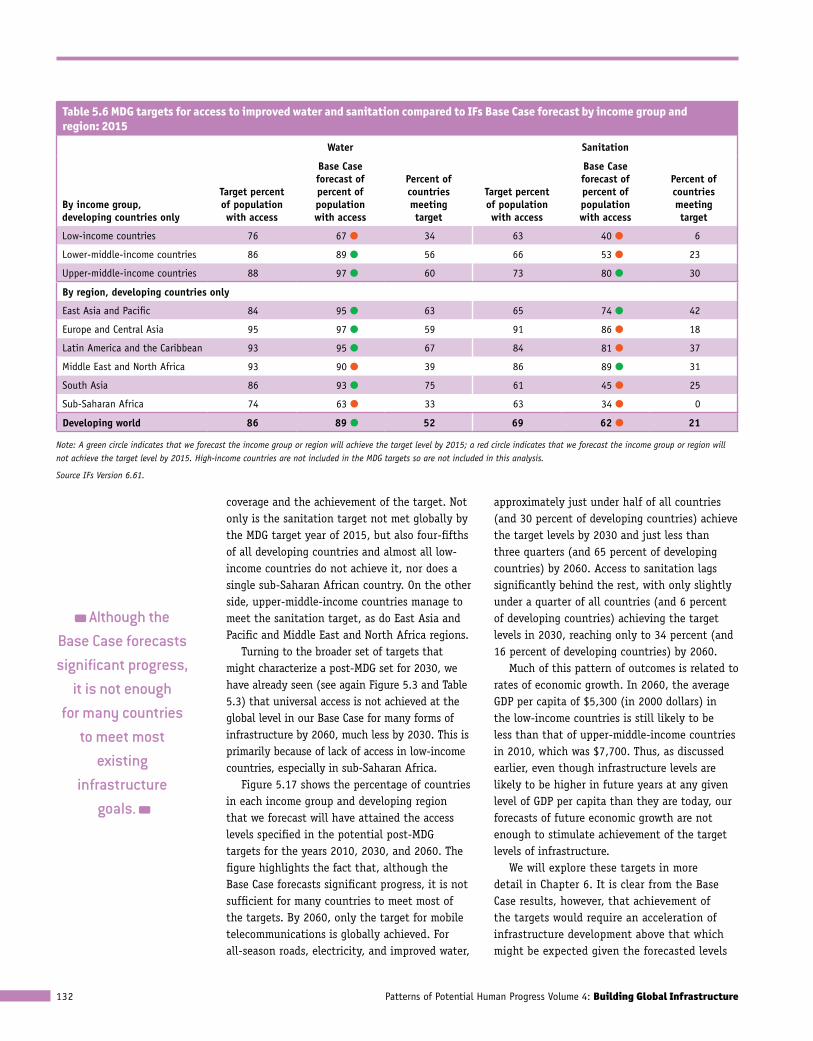
development, not necessarily what we might desire. Nonetheless, in our Base Case forecast, the MDG target for access to improved water will be met at the global level13 and by both of the middle-income country groups (Table 5.6, on p. 132). However, these aggregates hide the fact that half of all developing countries, including two-thirds of the low-income countries, will not meet the target. Regionally, sub-Saharan Africa and the Middle East and North Africa as a whole will not achieve the target, but for very different reasons. Sub-Saharan Africa is currently far from the target, requiring it to bring improved water infrastructure to a large segment of its population. The Middle East and North Africa, on the other hand, already has quite high levels of access, so it will have to provide infrastructure for ever-smaller and more isolated pockets of population, which is more expensive than provision at lower levels of access.
The situation for access to improved sanitation is even less sanguine than that for water, both in terms of the absolute levels of
Box 5.3 Infrastructure access targets beyond the MDGs
Our intent in identifying infrastructure targets was to contribute to ongoing discussions by developing and evaluating a set of targets that encompass a wide range of core infrastructure categories. The targets we eventually selected, by category of infrastructure, are:
■■ Transportation: reduce by one-half the portion of rural populations living beyond 2 kilometers of an all-season road, with a maximum target level of 90 percent access (that is, if a reduction of one-half implies a target level above 90 percent access, we set the target level to 90 percent.
■■ Energy: provide universal access to electricity and eliminate unventilated indoor use of solid fuels.
■■ Water and sanitation: provide universal access to improved sources of water and sanitation.
■■ Information and communication technologies: provide universal access to mobile broadband, where we define universal access for this goal as 150 subscriptions per 100 persons.*
The reader may wonder why we do not target universal access for all-season roads. First, the goal originally stated by Roberts, KC, and Rastogi (2006: A–25) in their analysis for the World Bank was simply to work at reducing the portion of the
rural population without access. Second, as noted by Foster and Briceño-Garmendia (2010: 56), “Because of low population densities in rural Africa, raising this Rural Access Index to 100 percent for Africa would be essentially unaffordable.” This conclusion is supported by our analysis, which shows that the amount of road needed to increase access grows exponentially as access goes much above 80 percent. This gives rise to rapidly increasing costs with the pursuit of each additional percentage point of access, making attainment of universal all-season road access extraordinarily expensive for countries with widely dispersed low-density populations. Unlike roads, which by definition require “grid access,” electricity (with generators and increasingly with distributed renewable production), water (with wells or transport of water), sanitation (with cesspools), and mobile broadband can be “off-grid,” making the pursuit of truly universal access a more reasonable goal.
Finally, although universal targets mean 100 percent access (or 150 subscriptions per 100 persons for mobile broadband), in this chapter and the next, we use a 97.5 percent access rate as a proxy for assessing whether a country or region has effectively attained universal access.
*Based on the International Telecommunication Union’s ideal value of 150 mobile phone subscriptions per 100 persons used in their ICT Development Index (ITU 2009: 18).
Our Base Case does not assume any special push on infrastructure.
It is meant to forecast what we might expect, not
necessarily what we might desire.
Patterns of Potential Human Progress Volume 4: Building Global Infrastructure132
coverage and the achievement of the target. Not only is the sanitation target not met globally by the MDG target year of 2015, but also four-fifths of all developing countries and almost all low-income countries do not achieve it, nor does a single sub-Saharan African country. On the other side, upper-middle-income countries manage to meet the sanitation target, as do East Asia and Pacific and Middle East and North Africa regions.
Turning to the broader set of targets that might characterize a post-MDG set for 2030, we have already seen (see again Figure 5.3 and Table 5.3) that universal access is not achieved at the global level in our Base Case for many forms of infrastructure by 2060, much less by 2030. This is primarily because of lack of access in low-income countries, especially in sub-Saharan Africa.
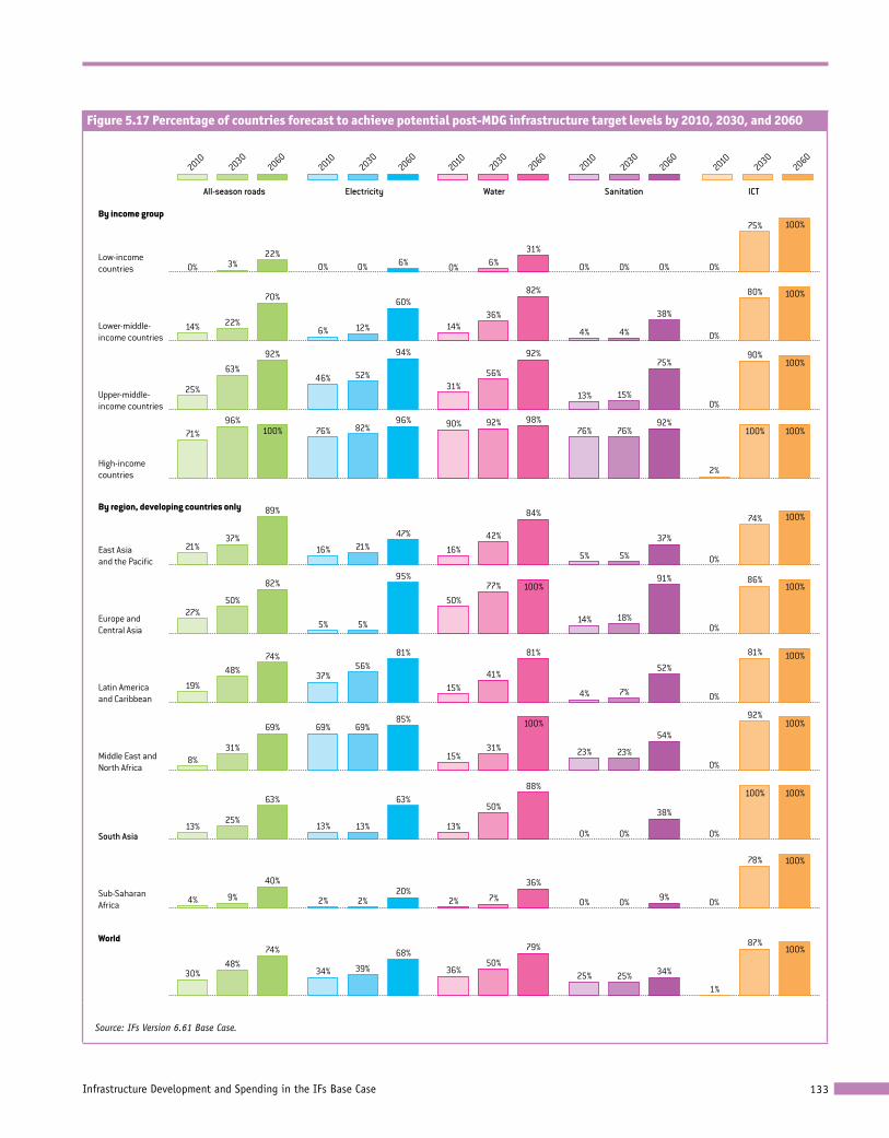
Figure 5.17 shows the percentage of countries in each income group and developing region that we forecast will have attained the access levels specified in the potential post-MDG targets for the years 2010, 2030, and 2060. The figure highlights the fact that, although the Base Case forecasts significant progress, it is not sufficient for many countries to meet most of the targets. By 2060, only the target for mobile telecommunications is globally achieved. For all-season roads, electricity, and improved water,
approximately just under half of all countries (and 30 percent of developing countries) achieve the target levels by 2030 and just less than three quarters (and 65 percent of developing countries) by 2060. Access to sanitation lags significantly behind the rest, with only slightly under a quarter of all countries (and 6 percent of developing countries) achieving the target levels in 2030, reaching only to 34 percent (and 16 percent of developing countries) by 2060.
Much of this pattern of outcomes is related to rates of economic growth. In 2060, the average GDP per capita of $5,300 (in 2000 dollars) in the low-income countries is still likely to be less than that of upper-middle-income countries in 2010, which was $7,700. Thus, as discussed earlier, even though infrastructure levels are likely to be higher in future years at any given level of GDP per capita than they are today, our forecasts of future economic growth are not enough to stimulate achievement of the target levels of infrastructure.
We will explore these targets in more detail in Chapter 6. It is clear from the Base Case results, however, that achievement of the targets would require an acceleration of infrastructure development above that which might be expected given the forecasted levels
Although the Base Case forecasts significant progress,
it is not enough for many countries
to meet most existing
infrastructure goals.
Table 5.6 MDG targets for access to improved water and sanitation compared to IFs Base Case forecast by income group and region: 2015
Water sanitation
By income group, developing countries only
target percent of population with access
Base case forecast of percent of population with access
Percent of countries meeting target
target percent of population with access
Base case forecast of percent of population with access
Percent of countries meeting target
Low-income countries 76 67 l 34 63 40 l 6
Lower-middle-income countries 86 89 l 56 66 53 l 23
Upper-middle-income countries 88 97 l 60 73 80 l 30
By region, developing countries only
East Asia and Pacific 84 95 l 63 65 74 l 42
Europe and Central Asia 95 97 l 59 91 86 l 18
Latin America and the Caribbean 93 95 l 67 84 81 l 37
Middle East and North Africa 93 90 l 39 86 89 l 31
South Asia 86 93 l 75 61 45 l 25
Sub-Saharan Africa 74 63 l 33 63 34 l 0
developing world 86 89 l 52 69 62 l 21
Note: A green circle indicates that we forecast the income group or region will achieve the target level by 2015; a red circle indicates that we forecast the income group or region will not achieve the target level by 2015. High-income countries are not included in the MDG targets so are not included in this analysis.
Source IFs Version 6.61.
Infrastructure Development and Spending in the IFs Base Case 133
Figure 5.17 Percentage of countries forecast to achieve potential post-MDG infrastructure target levels by 2010, 2030, and 2060
By income group
By region, developing countries only
Low-income countries
Upper-middle-income countries
Lower-middle-income countries
High-income countries
East Asia and the Paci�c
Europe and Central Asia
Latin America and Caribbean
South Asia
Sub-Saharan Africa
World
Middle East and North Africa
All-season roads
3%22%
22%14%
0%
70%
6%31%
36%14%
0%
82%
56%31%
92%
4%4%
38%
0%0% 0%
15%13%
75%
75%
90%
100%
2%
0%
0%
0%
0%
0%
0%
0%
0%
0%
80%
100%
100%
100%
100%
100%
100%
100%
100%
100%
100%
100%
6%
60%
12%6%
0%0%
63%
25%
92% 94%
52%46%
42%16%
84%
77%
41%
31%
50%
7%
50%
50%
15%
15%
13%
2%
36%
100%
81%
100%
88%
36%
79%
5%5%
37%
18%14%
91%
7%4%
52%
23%23%
54%
25%25%
0%0%
0%0%
34%
38%
9%
74%
86%
81%
92%
100%
78%
87%
1%
37%
50%
48%
31%
25%
9%
48%
21%
27%
19%
8%
13%
4%
30%
89%
82%
74%
69%
63%
40%
74%
47%
95%
81%
85%
63%
20%
68%
21%
5%
56%
69%
13%
2%
39%
16%
5%
37%
69%
13%
2%
34%
92%90% 98%76%76%
92%96%71% 100%
96%82%76%
Electricity Water Sanitation ICT
20102030
20602010
20302060
20102030
20602010
20302060
20102030
2060
Source: IFs Version 6.61 Base Case.
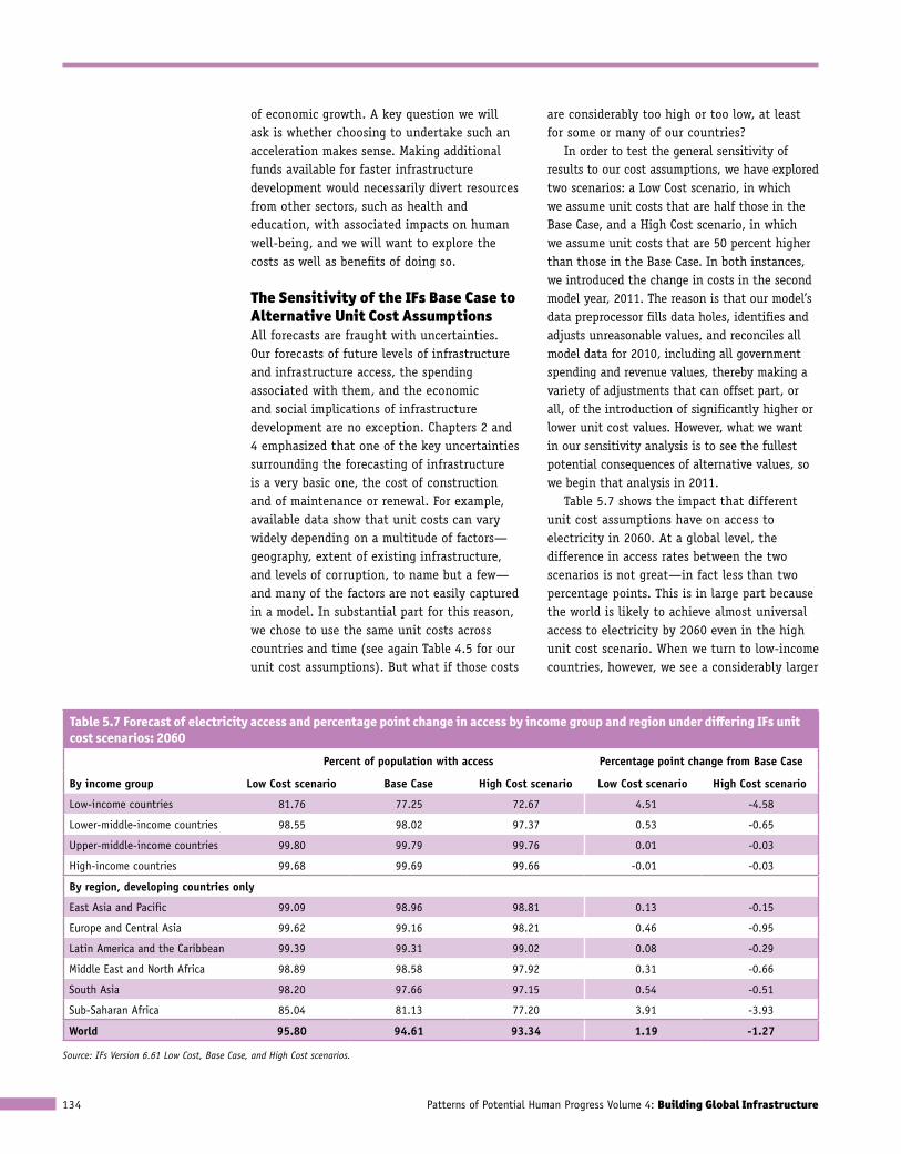
Patterns of Potential Human Progress Volume 4: Building Global Infrastructure134
of economic growth. A key question we will ask is whether choosing to undertake such an acceleration makes sense. Making additional funds available for faster infrastructure development would necessarily divert resources from other sectors, such as health and education, with associated impacts on human well-being, and we will want to explore the costs as well as benefits of doing so.
The Sensitivity of the IFs Base Case to Alternative Unit Cost AssumptionsAll forecasts are fraught with uncertainties. Our forecasts of future levels of infrastructure and infrastructure access, the spending associated with them, and the economic and social implications of infrastructure development are no exception. Chapters 2 and 4 emphasized that one of the key uncertainties surrounding the forecasting of infrastructure is a very basic one, the cost of construction and of maintenance or renewal. For example, available data show that unit costs can vary widely depending on a multitude of factors—geography, extent of existing infrastructure, and levels of corruption, to name but a few—and many of the factors are not easily captured in a model. In substantial part for this reason, we chose to use the same unit costs across countries and time (see again Table 4.5 for our unit cost assumptions). But what if those costs
are considerably too high or too low, at least for some or many of our countries?
In order to test the general sensitivity of results to our cost assumptions, we have explored two scenarios: a Low Cost scenario, in which we assume unit costs that are half those in the Base Case, and a High Cost scenario, in which we assume unit costs that are 50 percent higher than those in the Base Case. In both instances, we introduced the change in costs in the second model year, 2011. The reason is that our model’s data preprocessor fills data holes, identifies and adjusts unreasonable values, and reconciles all model data for 2010, including all government spending and revenue values, thereby making a variety of adjustments that can offset part, or all, of the introduction of significantly higher or lower unit cost values. However, what we want in our sensitivity analysis is to see the fullest potential consequences of alternative values, so we begin that analysis in 2011.
Table 5.7 shows the impact that different unit cost assumptions have on access to electricity in 2060. At a global level, the difference in access rates between the two scenarios is not great—in fact less than two percentage points. This is in large part because the world is likely to achieve almost universal access to electricity by 2060 even in the high unit cost scenario. When we turn to low-income countries, however, we see a considerably larger
Table 5.7 Forecast of electricity access and percentage point change in access by income group and region under differing IFs unit cost scenarios: 2060
By income group
Percent of population with access Percentage point change from Base case
low cost scenario Base case high cost scenario low cost scenario high cost scenario
Low-income countries 81.76 77.25 72.67 4.51 -4.58
Lower-middle-income countries 98.55 98.02 97.37 0.53 -0.65
Upper-middle-income countries 99.80 99.79 99.76 0.01 -0.03
High-income countries 99.68 99.69 99.66 -0.01 -0.03
By region, developing countries only
East Asia and Pacific 99.09 98.96 98.81 0.13 -0.15
Europe and Central Asia 99.62 99.16 98.21 0.46 -0.95
Latin America and the Caribbean 99.39 99.31 99.02 0.08 -0.29
Middle East and North Africa 98.89 98.58 97.92 0.31 -0.66
South Asia 98.20 97.66 97.15 0.54 -0.51
Sub-Saharan Africa 85.04 81.13 77.20 3.91 -3.93
World 95.80 94.61 93.34 1.19 -1.27
Source: IFs Version 6.61 Low Cost, Base Case, and High Cost scenarios.
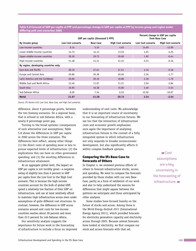
Infrastructure Development and Spending in the IFs Base Case 135
difference, about 9 percentage points, between the two framing scenarios. On a regional basis, that is echoed in sub-Saharan Africa, with a nearly 8 percentage point gap.
Turning to the broad systemic consequences of such alternative cost assumptions, Table 5.8 shows the differences in GDP per capita in 2060 across the three scenarios. The differences here reflect, among other things (1) the direct costs of spending more or less to pursue expected levels of infrastructure; (2) the implications this can have on other government spending; and (3) the resulting differences in infrastructure attainment.
At an aggregate global level, the impact on GDP per capita is not terribly great—a negative swing of slightly less than 6 percent in GDP per capita from the Low Cost to the High Cost scenario. This is because the high-income countries account for the bulk of global GDP, spend a relatively low fraction of their GDP on infrastructure, and can at least relatively afford to maintain high infrastructure access even under assumptions of quite different cost structures. In contrast, however, the difference in GDP across scenarios around unit costs for low-income countries reaches about 28 percent and more than 23.5 percent for sub-Saharan Africa.
Our sensitivity analysis suggests the importance for future work in the forecasting of infrastructure to include a focus on improved
understanding of unit costs. We acknowledge that it is an important source of uncertainty in our forecasting of infrastructure futures. We see too that the interaction of infrastructure costs and economic growth emphasizes once again the importance of analyzing infrastructure futures in the context of a fully integrated system in which infrastructure not only responds to broader socioeconomic development, but also significantly affects it within complex feedback systems.
Comparing the IFs Base Case to Forecasts of OthersIn Chapter 4, we reviewed previous efforts of others to forecast infrastructure stocks, access, and spending. We want to compare the forecasts provided by those studies with our own Base Case, partly as a form of validation of our work and also to help understand the reasons for differences that might appear between the patterns we anticipate and those anticipated by other analyses.
Some studies have focused heavily on the future of stocks and access. Among those is the World Energy Outlook 2011 (International Energy Agency 2011), which provided forecasts for electricity generation capacity and electricity access through 2025. Because several forecasts have looked at electricity, we first compare our stock and access forecasts with that set.
Table 5.8 Forecast of GDP per capita at PPP and percentage change in GDP per capita at PPP by income group and region under differing unit cost scenarios: 2060
By income group
gdP per capita (thousand $ PPP)Percent change in gdP per capita
from Base case
low cost scenario Base case high cost scenario low cost scenario high cost scenario
Low-income countries 6.14 5.34 4.65 14.99 -12.99
Lower-middle-income countries 14.72 14.12 13.52 4.25 -4.25
Upper-middle-income countries 30.30 29.73 29.60 1.92 -0.44
High-income countries 51.48 51.31 51.23 0.33 -0.16
By region, developing countries only
East Asia and Pacific 28.19 27.61 27.51 2.10 -0.36
Europe and Central Asia 20.86 20.38 20.02 2.36 -1.77
Latin America and the Caribbean 20.60 20.16 19.80 2.18 -1.79
Middle East and North Africa 12.40 11.97 11.51 3.59 -3.84
South Asia 16.95 16.38 15.80 3.48 -3.54
Sub-Saharan Africa 8.26 7.34 6.53 12.56 -10.97
World 21.97 21.28 20.74 3.24 -2.54
Source: IFs Version 6.61 Low Cost, Base Case, and High Cost scenarios.
Cost assumptions
are a key uncertainty in
the forecasting of infrastructure.
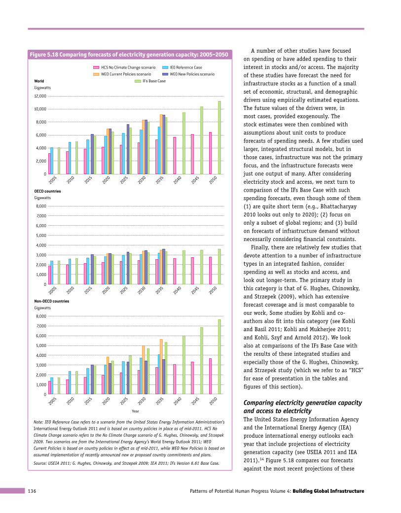
Patterns of Potential Human Progress Volume 4: Building Global Infrastructure136
A number of other studies have focused on spending or have added spending to their interest in stocks and/or access. The majority of these studies have forecast the need for infrastructure stocks as a function of a small set of economic, structural, and demographic drivers using empirically estimated equations. The future values of the drivers were, in most cases, provided exogenously. The stock estimates were then combined with assumptions about unit costs to produce forecasts of spending needs. A few studies used larger, integrated structural models, but in those cases, infrastructure was not the primary focus, and the infrastructure forecasts were just one output of many. After considering electricity stock and access, we next turn to comparison of the IFs Base Case with such spending forecasts, even though some of them (1) are quite short term (e.g., Bhattacharyay 2010 looks out only to 2020); (2) focus on only a subset of global regions; and (3) build on forecasts of infrastructure demand without necessarily considering financial constraints.
Finally, there are relatively few studies that devote attention to a number of infrastructure types in an integrated fashion, consider spending as well as stocks and access, and look out longer-term. The primary study in this category is that of G. Hughes, Chinowsky, and Strzepek (2009), which has extensive forecast coverage and is most comparable to our work, Some studies by Kohli and co-authors also fit into this category (see Kohli and Basil 2011; Kohli and Mukherjee 2011; and Kohli, Szyf and Arnold 2012). We look also at comparisons of the IFs Base Case with the results of these integrated studies and especially those of the G. Hughes, Chinowsky, and Strzepek study (which we refer to as “HCS” for ease of presentation in the tables and figures of this section).
Comparing electricity generation capacity and access to electricityThe United States Energy Information Agency and the International Energy Agency (IEA) produce international energy outlooks each year that include projections of electricity generation capacity (see USEIA 2011 and IEA 2011).14 Figure 5.18 compares our forecasts against the most recent projections of these
Figure 5.18 Comparing forecasts of electricity generation capacity: 2005−2050
8,000
0
5,000
4,000
3,000
2,000
1,000
6,000
7,000
5,000
4,000
3,000
2,000
1,000
6,000
7,000
20052010
20402030
20452050
20352020
20252015
20052010
20402030
20452050
20352020
20252015
20052010
20402030
20452050
20352020
20252015
Year
WEO Current Policies scenario
IFs Base Case
WEO New Policies scenario
GigawattsWorld
Gigawatts
Non-OECD countries
12,000
0
GigawattsOECD countries
8,000
4,000
2,000
6,000
8,000
10,000
0
IEO Reference CaseHCS No Climate Change scenario
Note: IEO Reference Case refers to a scenario from the United States Energy Information Administration’s International Energy Outlook 2011 and is based on country policies in place as of mid-2011. HCS No Climate Change scenario refers to the No Climate Change scenario of G. Hughes, Chinowsky, and Strzepek 2009. Two scenarios are from the International Energy Agency’s World Energy Outlook 2011; WEO Current Policies is based on country policies in effect as of mid-2011, while WEO New Policies is based on assumed implementation of recently announced new or proposed country commitments and plans.
Source: USEIA 2011; G. Hughes, Chinowsky, and Strzepek 2009; IEA 2011; IFs Version 6.61 Base Case.
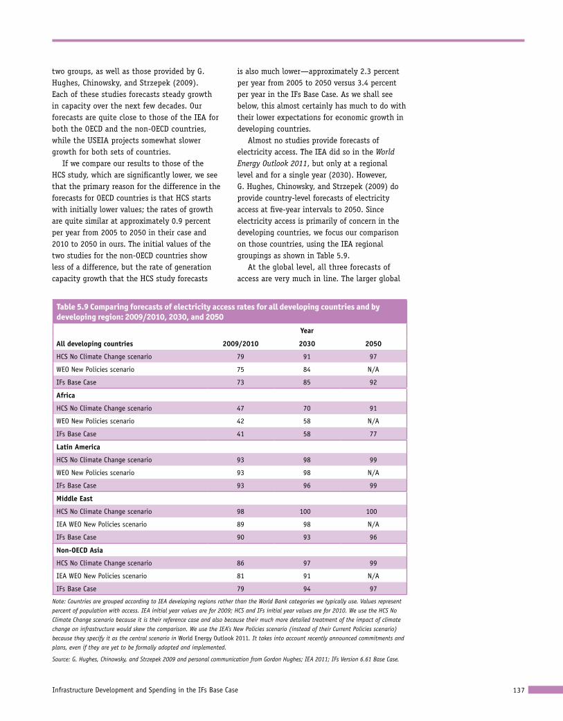
Infrastructure Development and Spending in the IFs Base Case 137
two groups, as well as those provided by G. Hughes, Chinowsky, and Strzepek (2009). Each of these studies forecasts steady growth in capacity over the next few decades. Our forecasts are quite close to those of the IEA for both the OECD and the non-OECD countries, while the USEIA projects somewhat slower growth for both sets of countries.
If we compare our results to those of the HCS study, which are significantly lower, we see that the primary reason for the difference in the forecasts for OECD countries is that HCS starts with initially lower values; the rates of growth are quite similar at approximately 0.9 percent per year from 2005 to 2050 in their case and 2010 to 2050 in ours. The initial values of the two studies for the non-OECD countries show less of a difference, but the rate of generation capacity growth that the HCS study forecasts
is also much lower—approximately 2.3 percent per year from 2005 to 2050 versus 3.4 percent per year in the IFs Base Case. As we shall see below, this almost certainly has much to do with their lower expectations for economic growth in developing countries.
Almost no studies provide forecasts of electricity access. The IEA did so in the World Energy Outlook 2011, but only at a regional level and for a single year (2030). However, G. Hughes, Chinowsky, and Strzepek (2009) do provide country-level forecasts of electricity access at five-year intervals to 2050. Since electricity access is primarily of concern in the developing countries, we focus our comparison on those countries, using the IEA regional groupings as shown in Table 5.9.
At the global level, all three forecasts of access are very much in line. The larger global
Table 5.9 Comparing forecasts of electricity access rates for all developing countries and by developing region: 2009/2010, 2030, and 2050
all developing countries
Year
2009/2010 2030 2050
HCS No Climate Change scenario 79 91 97
WEO New Policies scenario 75 84 N/A
IFs Base Case 73 85 92
africa
HCS No Climate Change scenario 47 70 91
WEO New Policies scenario 42 58 N/A
IFs Base Case 41 58 77
latin america
HCS No Climate Change scenario 93 98 99
WEO New Policies scenario 93 98 N/A
IFs Base Case 93 96 99
Middle east
HCS No Climate Change scenario 98 100 100
IEA WEO New Policies scenario 89 98 N/A
IFs Base Case 90 93 96
non-oecd asia
HCS No Climate Change scenario 86 97 99
IEA WEO New Policies scenario 81 91 N/A
IFs Base Case 79 94 97
Note: Countries are grouped according to IEA developing regions rather than the World Bank categories we typically use. Values represent percent of population with access. IEA initial year values are for 2009; HCS and IFs initial year values are for 2010. We use the HCS No Climate Change scenario because it is their reference case and also because their much more detailed treatment of the impact of climate change on infrastructure would skew the comparison. We use the IEA’s New Policies scenario (instead of their Current Policies scenario) because they specify it as the central scenario in World Energy Outlook 2011. It takes into account recently announced commitments and plans, even if they are yet to be formally adopted and implemented.
Source: G. Hughes, Chinowsky, and Strzepek 2009 and personal communication from Gordon Hughes; IEA 2011; IFs Version 6.61 Base Case.
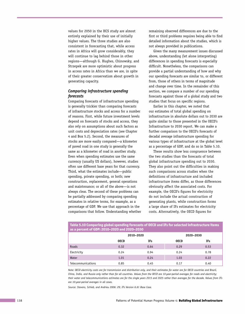
Patterns of Potential Human Progress Volume 4: Building Global Infrastructure138
values for 2050 in the HCS study are almost entirely explained by their use of initially higher values. The three studies are also consistent in forecasting that, while access rates in Africa will grow considerably, they will continue to lag behind those in other regions—although G. Hughes, Chinowsky, and Strzepek are more optimistic about progress in access rates in Africa than we are, in spite of their greater conservatism about growth in generating capacity.
Comparing infrastructure spending forecastsComparing forecasts of infrastructure spending is generally trickier than comparing forecasts of infrastructure stocks and access for a number of reasons. First, while future investment levels depend on forecasts of stocks and access, they also rely on assumptions about such factors as unit costs and depreciation rates (see Chapter 4 and Box 5.2). Second, the measures of stocks are more easily compared—a kilometer of paved road in one study is generally the same as a kilometer of road in another study. Even when spending estimates use the same currency (usually US dollars), however, studies often use different base years for that currency. Third, what the estimates include—public spending, private spending, or both; new construction, replacement, general operations and maintenance; or all of the above—is not always clear. The second of these problems can be partially addressed by comparing spending estimates in relative terms, for example, as a percentage of GDP. We use that approach in the comparisons that follow. Understanding whether
remaining observed differences are due to the first or third problems requires being able to find detailed information about the studies, which is not always provided in publications.
Given the many measurement issues discussed above, understanding (let alone interpreting) differences in spending forecasts is especially difficult. Nonetheless, the comparisons can provide a partial understanding of how and why our spending forecasts are similar to, or different from, those of others in terms of magnitude and change over time. In the remainder of this section, we compare a number of our spending forecasts against those of a global study and two studies that focus on specific regions.
Earlier in this chapter, we noted that our estimates of total global spending on infrastructure in absolute dollars out to 2030 are quite similar to those presented in the OECD’s Infrastructure to 2030 report. We can make a further comparison to the OECD’s forecasts of decadal average infrastructure spending for various types of infrastructure at the global level as a percentage of GDP, and do so in Table 5.10.
These results show less congruence between the two studies than the forecasts of total global infrastructure spending out to 2030. They also point out the difficulties in making such comparisons across studies when the definitions of infrastructure and included infrastructure items differ, as those differences obviously affect the associated costs. For example, the OECD’s figures for electricity do not include the actual construction of generating plants, while construction forms a large share of IFs estimates for electricity costs. Alternatively, the OECD figures for
Table 5.10 Comparing global spending forecasts of OECD and IFs for selected infrastructure items as a percent of GDP: 2010–2020 and 2020–2030
2010–2020 2020–2030
oecd ifs oecd ifs
Roads 0.32 0.64 0.29 0.53
Electricity 0.24 0.94 0.24 0.78
Water 1.01 0.24 1.03 0.22
Telecommunications 0.85 0.45 0.17 0.40
Note: OECD electricity costs are for transmission and distribution only, and their estimates for water are for OECD countries and Brazil, China, India, and Russia only rather than for all countries. Values from the OECD are 10-year-period averages for roads and electricity; their water and telecommunications estimates are for the single years 2015 and 2025 rather than averages for the decade. Values from IFs are 10-year-period averages in all cases.
Source: Stevens, Schieb, and Andrieu 2006: 29; IFs Version 6.61 Base Case.
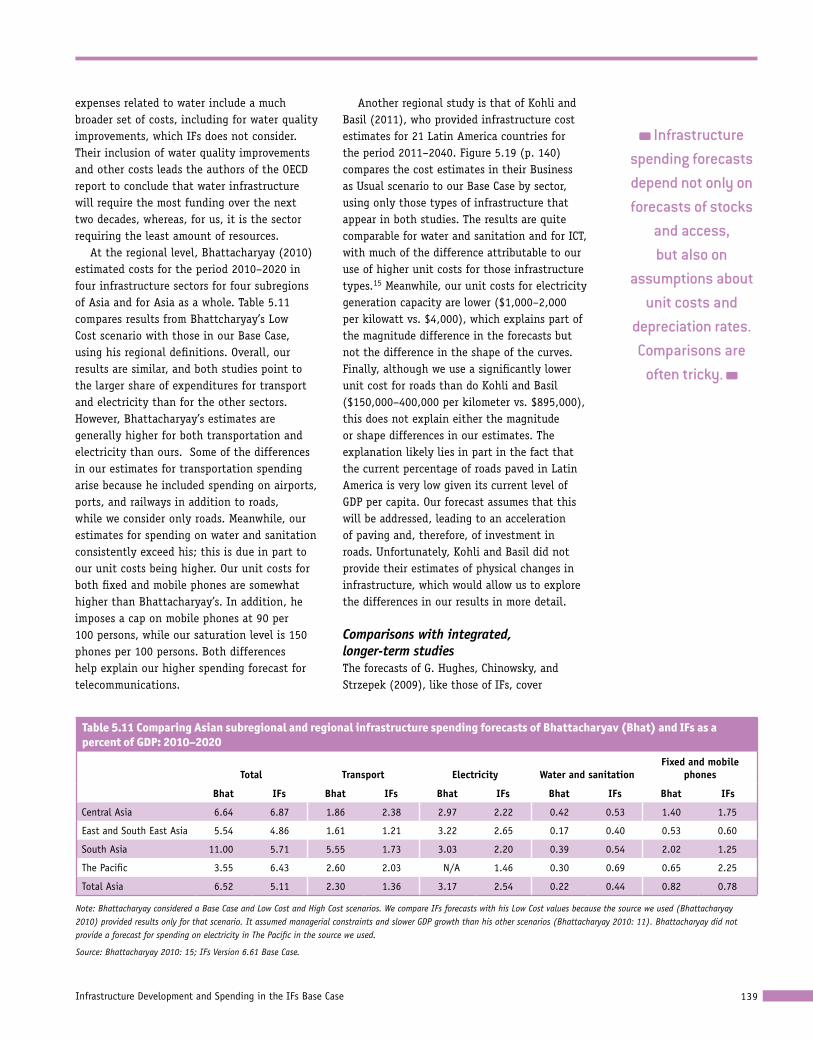
Infrastructure Development and Spending in the IFs Base Case 139
Infrastructure spending forecasts depend not only on forecasts of stocks
and access, but also on
assumptions about unit costs and
depreciation rates. Comparisons are
often tricky.
expenses related to water include a much broader set of costs, including for water quality improvements, which IFs does not consider. Their inclusion of water quality improvements and other costs leads the authors of the OECD report to conclude that water infrastructure will require the most funding over the next two decades, whereas, for us, it is the sector requiring the least amount of resources.
At the regional level, Bhattacharyay (2010) estimated costs for the period 2010–2020 in four infrastructure sectors for four subregions of Asia and for Asia as a whole. Table 5.11 compares results from Bhattcharyay’s Low Cost scenario with those in our Base Case, using his regional definitions. Overall, our results are similar, and both studies point to the larger share of expenditures for transport and electricity than for the other sectors. However, Bhattacharyay’s estimates are generally higher for both transportation and electricity than ours. Some of the differences in our estimates for transportation spending arise because he included spending on airports, ports, and railways in addition to roads, while we consider only roads. Meanwhile, our estimates for spending on water and sanitation consistently exceed his; this is due in part to our unit costs being higher. Our unit costs for both fixed and mobile phones are somewhat higher than Bhattacharyay’s. In addition, he imposes a cap on mobile phones at 90 per 100 persons, while our saturation level is 150 phones per 100 persons. Both differences help explain our higher spending forecast for telecommunications.
Another regional study is that of Kohli and Basil (2011), who provided infrastructure cost estimates for 21 Latin America countries for the period 2011–2040. Figure 5.19 (p. 140) compares the cost estimates in their Business as Usual scenario to our Base Case by sector, using only those types of infrastructure that appear in both studies. The results are quite comparable for water and sanitation and for ICT, with much of the difference attributable to our use of higher unit costs for those infrastructure types.15 Meanwhile, our unit costs for electricity generation capacity are lower ($1,000–2,000 per kilowatt vs. $4,000), which explains part of the magnitude difference in the forecasts but not the difference in the shape of the curves. Finally, although we use a significantly lower unit cost for roads than do Kohli and Basil ($150,000–400,000 per kilometer vs. $895,000), this does not explain either the magnitude or shape differences in our estimates. The explanation likely lies in part in the fact that the current percentage of roads paved in Latin America is very low given its current level of GDP per capita. Our forecast assumes that this will be addressed, leading to an acceleration of paving and, therefore, of investment in roads. Unfortunately, Kohli and Basil did not provide their estimates of physical changes in infrastructure, which would allow us to explore the differences in our results in more detail.
Comparisons with integrated, longer-term studies The forecasts of G. Hughes, Chinowsky, and Strzepek (2009), like those of IFs, cover
Table 5.11 Comparing Asian subregional and regional infrastructure spending forecasts of Bhattacharyav (Bhat) and IFs as a percent of GDP: 2010–2020
total transport electricity Water and sanitationfixed and mobile
phones
Bhat ifs Bhat ifs Bhat ifs Bhat ifs Bhat ifs
Central Asia 6.64 6.87 1.86 2.38 2.97 2.22 0.42 0.53 1.40 1.75
East and South East Asia 5.54 4.86 1.61 1.21 3.22 2.65 0.17 0.40 0.53 0.60
South Asia 11.00 5.71 5.55 1.73 3.03 2.20 0.39 0.54 2.02 1.25
The Pacific 3.55 6.43 2.60 2.03 N/A 1.46 0.30 0.69 0.65 2.25
Total Asia 6.52 5.11 2.30 1.36 3.17 2.54 0.22 0.44 0.82 0.78
Note: Bhattacharyay considered a Base Case and Low Cost and High Cost scenarios. We compare IFs forecasts with his Low Cost values because the source we used (Bhattacharyay 2010) provided results only for that scenario. It assumed managerial constraints and slower GDP growth than his other scenarios (Bhattacharyay 2010: 11). Bhattacharyay did not provide a forecast for spending on electricity in The Pacific in the source we used.
Source: Bhattacharyay 2010: 15; IFs Version 6.61 Base Case.
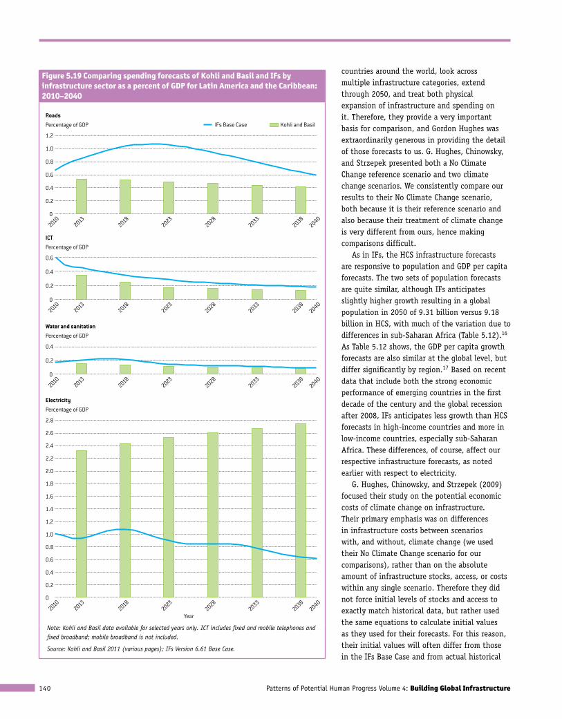
Patterns of Potential Human Progress Volume 4: Building Global Infrastructure140
countries around the world, look across multiple infrastructure categories, extend through 2050, and treat both physical expansion of infrastructure and spending on it. Therefore, they provide a very important basis for comparison, and Gordon Hughes was extraordinarily generous in providing the detail of those forecasts to us. G. Hughes, Chinowsky, and Strzepek presented both a No Climate Change reference scenario and two climate change scenarios. We consistently compare our results to their No Climate Change scenario, both because it is their reference scenario and also because their treatment of climate change is very different from ours, hence making comparisons difficult.
As in IFs, the HCS infrastructure forecasts are responsive to population and GDP per capita forecasts. The two sets of population forecasts are quite similar, although IFs anticipates slightly higher growth resulting in a global population in 2050 of 9.31 billion versus 9.18 billion in HCS, with much of the variation due to differences in sub-Saharan Africa (Table 5.12).16 As Table 5.12 shows, the GDP per capita growth forecasts are also similar at the global level, but differ significantly by region.17 Based on recent data that include both the strong economic performance of emerging countries in the first decade of the century and the global recession after 2008, IFs anticipates less growth than HCS forecasts in high-income countries and more in low-income countries, especially sub-Saharan Africa. These differences, of course, affect our respective infrastructure forecasts, as noted earlier with respect to electricity.
G. Hughes, Chinowsky, and Strzepek (2009) focused their study on the potential economic costs of climate change on infrastructure. Their primary emphasis was on differences in infrastructure costs between scenarios with, and without, climate change (we used their No Climate Change scenario for our comparisons), rather than on the absolute amount of infrastructure stocks, access, or costs within any single scenario. Therefore they did not force initial levels of stocks and access to exactly match historical data, but rather used the same equations to calculate initial values as they used for their forecasts. For this reason, their initial values will often differ from those in the IFs Base Case and from actual historical
Figure 5.19 Comparing spending forecasts of Kohli and Basil and IFs by infrastructure sector as a percent of GDP for Latin America and the Caribbean: 2010–2040
20102018
20282040
20132023
20332038
IFs Base Case Kohli and Basil
Year
1.2
1.0
0.8
0.6
0.4
0.2
0
Percentage of GDP
Roads
20102018
20282040
20132023
20332038
0.6
0.4
0.2
0
Percentage of GDP
ICT
20102018
20282040
20132023
20332038
0.4
0.2
0
Percentage of GDP
Water and sanitation
20102018
20282040
20132023
20332038
2.8
2.6
2.4
2.2
2.0
1.8
1.6
1.4
1.2
1.0
0.8
0.6
0.4
0.2
0
Percentage of GDP
Electricity
Note: Kohli and Basil data available for selected years only. ICT includes fixed and mobile telephones and fixed broadband; mobile broadband is not included.
Source: Kohli and Basil 2011 (various pages); IFs Version 6.61 Base Case.
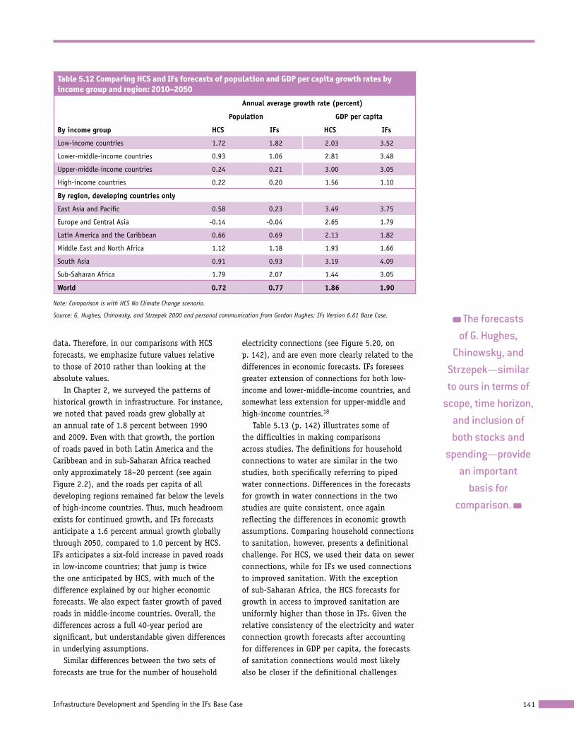
Infrastructure Development and Spending in the IFs Base Case 141
The forecasts of G. Hughes,
Chinowsky, and Strzepek—similar to ours in terms of
scope, time horizon, and inclusion of both stocks and
spending—provide an important
basis for comparison.
data. Therefore, in our comparisons with HCS forecasts, we emphasize future values relative to those of 2010 rather than looking at the absolute values.
In Chapter 2, we surveyed the patterns of historical growth in infrastructure. For instance, we noted that paved roads grew globally at an annual rate of 1.8 percent between 1990 and 2009. Even with that growth, the portion of roads paved in both Latin America and the Caribbean and in sub-Saharan Africa reached only approximately 18–20 percent (see again Figure 2.2), and the roads per capita of all developing regions remained far below the levels of high-income countries. Thus, much headroom exists for continued growth, and IFs forecasts anticipate a 1.6 percent annual growth globally through 2050, compared to 1.0 percent by HCS. IFs anticipates a six-fold increase in paved roads in low-income countries; that jump is twice the one anticipated by HCS, with much of the difference explained by our higher economic forecasts. We also expect faster growth of paved roads in middle-income countries. Overall, the differences across a full 40-year period are significant, but understandable given differences in underlying assumptions.
Similar differences between the two sets of forecasts are true for the number of household
electricity connections (see Figure 5.20, on p. 142), and are even more clearly related to the differences in economic forecasts. IFs foresees greater extension of connections for both low-income and lower-middle-income countries, and somewhat less extension for upper-middle and high-income countries.18
Table 5.13 (p. 142) illustrates some of the difficulties in making comparisons across studies. The definitions for household connections to water are similar in the two studies, both specifically referring to piped water connections. Differences in the forecasts for growth in water connections in the two studies are quite consistent, once again reflecting the differences in economic growth assumptions. Comparing household connections to sanitation, however, presents a definitional challenge. For HCS, we used their data on sewer connections, while for IFs we used connections to improved sanitation. With the exception of sub-Saharan Africa, the HCS forecasts for growth in access to improved sanitation are uniformly higher than those in IFs. Given the relative consistency of the electricity and water connection growth forecasts after accounting for differences in GDP per capita, the forecasts of sanitation connections would most likely also be closer if the definitional challenges
Table 5.12 Comparing HCS and IFs forecasts of population and GDP per capita growth rates by income group and region: 2010–2050
By income group
annual average growth rate (percent)
Population gdP per capita
hcs ifs hcs ifs
Low-income countries 1.72 1.82 2.03 3.52
Lower-middle-income countries 0.93 1.06 2.81 3.48
Upper-middle-income countries 0.24 0.21 3.00 3.05
High-income countries 0.22 0.20 1.56 1.10
By region, developing countries only
East Asia and Pacific 0.58 0.23 3.49 3.75
Europe and Central Asia -0.14 -0.04 2.65 1.79
Latin America and the Caribbean 0.66 0.69 2.13 1.82
Middle East and North Africa 1.12 1.18 1.93 1.66
South Asia 0.91 0.93 3.19 4.09
Sub-Saharan Africa 1.79 2.07 1.44 3.05
World 0.72 0.77 1.86 1.90
Note: Comparison is with HCS No Climate Change scenario.
Source: G. Hughes, Chinowsky, and Strzepek 2000 and personal communication from Gordon Hughes; IFs Version 6.61 Base Case.
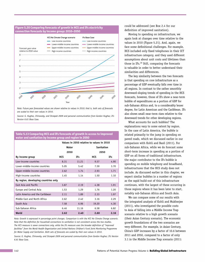
Patterns of Potential Human Progress Volume 4: Building Global Infrastructure142
could be addressed (see Box 2.4 for our definition of improved sanitation).
Moving to spending on infrastructure, we again look at changes over time relative to the values in 2010 (Figure 5.21). And, again, we face some definitional challenges. For example, HCS included only fixed telephones in their ICT infrastructure category, and they used different assumptions about unit costs and lifetimes than those in IFs.19 Still, comparing the forecasts is valuable in order to better understand their similarities and differences.
The key similarity between the two forecasts is that spending on core infrastructure as a percentage of GDP eventually falls over time in all regions. In contrast to the rather smoothly downward-sloping trends of spending in the HCS forecasts, however, those of IFs show a near-term bubble of expenditures as a portion of GDP for sub-Saharan Africa and, to a considerably lesser degree, for Latin American and the Caribbean. IFs also shows small near-term rises relative to the downward trends for other developing regions.
What accounts for such bubbles? The explanations vary to some extent by region. In the case of Latin America, the bubble is related primarily to the jump in spending on paved roads, which we discussed earlier in our comparison with Kohli and Basil (2011). For sub-Saharan Africa, while we do forecast some short-term increase in spending as a portion of GDP on all forms of traditional infrastructure, the major contributor to the IFs bubble is spending on mobile telephony and broadband, infrastructures that the HCS study does not include. As discussed earlier in this chapter, we expect similar bubbles in a number of regions as the rapid build-out of this infrastructure continues, with the largest of these occurring in those regions where it has been later to start, notably sub-Saharan Africa and South Asia.
We can compare some of our results with the integrated analysis of Kohli and Mukherjee (2011), who investigated the possible costs to Asia of falling into a Middle Income Trap scenario relative to a high growth scenario (their Asian Century scenario). The economic growth foundations of the two scenarios are very different. For example, in Asian Century, China’s GDP increases by a factor of 10.6 between 2011 and 2050, compared to a factor of only 3.1 in the Middle Income Trap scenario (2011:
Figure 5.20 Comparing forecasts of growth in HCS and IFs electricity connection forecasts by income group: 2010–2050
IFs Base CaseHCS No Climate Change scenario
Low-income countriesLower-middle-income countriesUpper-middle-income countries
High-income countries
Low-income countriesLower-middle-income countriesUpper-middle-income countries
High-income countriesForecast year value relative to 2010 value
8
1
2
3
4
5
6
7
20102050
20402030
20452035
20202025
2015
Year
Note: Future year forecasted values are shown relative to values in 2010; that is, both sets of forecasts are scaled to their own values in 2010.
Source: G. Hughes, Chinowsky, and Strzepek 2009 and personal communication from Gordon Hughes; IFs Version 6.61 Base Case.
Table 5.13 Comparing HCS and IFs forecasts of growth in access to improved water and sanitation by income group and region in 2050
By income group
Values in 2050 relative to values in 2010
Water sanitation
2050 2050
hcs ifs hcs ifs
Low-income countries 8.31 11.21 9.57 4.90
Lower-middle-income countries 5.05 5.42 7.59 3.70
Upper-middle-income countries 2.62 1.74 2.93 1.71
High-income countries 1.45 1.14 1.50 1.10
By region, developing countries only
East Asia and Pacific 3.87 2.19 4.38 1.91
Europe and Central Asia 1.53 1.29 1.76 1.20
Latin America and the Caribbean 2.11 1.89 2.33 1.97
Middle East and North Africa 2.62 2.42 3.16 2.29
South Asia 7.58 6.96 19.20 4.30
Sub-Saharan Africa 6.46 11.16 6.58 6.82
World 2.62 2.40 2.60 2.16
Note: Growth is expressed in percentage point changes. Comparison is with the HCS No Climate Change scenario. Note that the definition for household connections to sanitation is not consistent across the two studies. The HCS measure is sewer connections only, while the IFs measure uses the broader definition of “improved facilities” from the World Health Organization and United Nations Children’s Fund Joint Monitoring Programme for Water Supply and Sanitation. Both sets of forecasts are scaled by their own values in 2010.
Source: G. Hughes, Chinowsky, and Strzepek 2009 and personal communication from Gordon Hughes; IFs Version 6.61 Base Case.
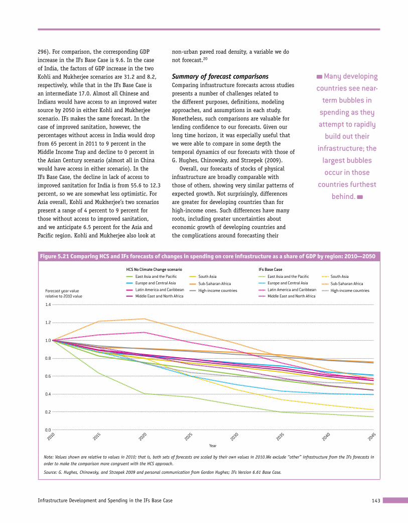
Infrastructure Development and Spending in the IFs Base Case 143
296). For comparison, the corresponding GDP increase in the IFs Base Case is 9.6. In the case of India, the factors of GDP increase in the two Kohli and Mukherjee scenarios are 31.2 and 8.2, respectively, while that in the IFs Base Case is an intermediate 17.0. Almost all Chinese and Indians would have access to an improved water source by 2050 in either Kohli and Mukherjee scenario. IFs makes the same forecast. In the case of improved sanitation, however, the percentages without access in India would drop from 65 percent in 2011 to 9 percent in the Middle Income Trap and decline to 0 percent in the Asian Century scenario (almost all in China would have access in either scenario). In the IFs Base Case, the decline in lack of access to improved sanitation for India is from 55.6 to 12.3 percent, so we are somewhat less optimistic. For Asia overall, Kohli and Mukherjee’s two scenarios present a range of 4 percent to 9 percent for those without access to improved sanitation, and we anticipate 6.5 percent for the Asia and Pacific region. Kohli and Mukherjee also look at
non-urban paved road density, a variable we do not forecast.20
Summary of forecast comparisons Comparing infrastructure forecasts across studies presents a number of challenges related to the different purposes, definitions, modeling approaches, and assumptions in each study. Nonetheless, such comparisons are valuable for lending confidence to our forecasts. Given our long time horizon, it was especially useful that we were able to compare in some depth the temporal dynamics of our forecasts with those of G. Hughes, Chinowsky, and Strzepek (2009).
Overall, our forecasts of stocks of physical infrastructure are broadly comparable with those of others, showing very similar patterns of expected growth. Not surprisingly, differences are greater for developing countries than for high-income ones. Such differences have many roots, including greater uncertainties about economic growth of developing countries and the complications around forecasting their
Many developing countries see near-
term bubbles in spending as they attempt to rapidly
build out their infrastructure; the
largest bubbles occur in those
countries furthest behind.
Figure 5.21 Comparing HCS and IFs forecasts of changes in spending on core infrastructure as a share of GDP by region: 2010—2050
IFs Base CaseHCS No Climate Change scenario
East Asia and the Paci�cEurope and Central AsiaLatin America and Caribbean
South AsiaEast Asia and the Paci�cEurope and Central AsiaLatin America and Caribbean
South Asia
Sub-Saharan Africa
High-income countries
Sub-Saharan Africa
Middle East and North Africa Middle East and North Africa High-income countriesForecast year value
relative to 2010 value
1.4
0.0
0.2
0.4
0.6
0.8
1.0
1.2
20102040
20302045
20352020
20252015
Year
Note: Values shown are relative to values in 2010; that is, both sets of forecasts are scaled by their own values in 2010.We exclude “other” infrastructure from the IFs forecasts in order to make the comparison more congruent with the HCS approach.
Source: G. Hughes, Chinowsky, and Strzepek 2009 and personal communication from Gordon Hughes; IFs Version 6.61 Base Case.
Patterns of Potential Human Progress Volume 4: Building Global Infrastructure144
degree of attention to infrastructure given the many competing demands for their resources.
With respect to spending on infrastructure, the forecasts made by IFs and other studies differ more significantly. Yet, especially when considering the sometimes very different specifications of the infrastructure analyzed, of the unit costs, and presumably (but not always explicitly) of underlying physical system growth, the differences are generally reasonable. Furthermore, there tends to be agreement that, as countries become richer and complete their build-outs of systems, spending on core infrastructure as a share of GDP will decline. This also leads us generally to anticipate both lower shares of GDP directed to infrastructure in higher-income countries at any given point in time than in lower-income ones and decreasing shares of GDP spent within most countries over time (however, there can be bubbles of spending as a share of GDP for low-income countries as they accelerate the build-out process).
ConclusionOur Base Case forecast indicates that, over the next half century, we can expect countries to increase their stocks of core infrastructure as well as their rates of access to core infrastructure services, even as populations grow. Still, significant numbers of people will continue to lack access to basic infrastructure services. For example, we forecast that in 2060 approximately 250 million people will not have access to an improved source of drinking water, half a billion people will not have access to electricity or live within two kilometers of an all-season road, and 1 billion people will not have access to improved sanitation. The vast majority of these people will be in low-income and lower-middle-income countries in sub-
Saharan Africa and elsewhere. In fact, in the IFs Base Case, most developing countries will not achieve the proposed targets of universal, or near-universal, access to these services by 2030, and many will not achieve them even by 2060.
The formulations within IFs that determine the basic levels of infrastructure development that we expect are rooted in historical patterns of relationship between actual infrastructure development and the underlying drivers of it, such as population and income size. Thus, our forecasts are not of some unconstrained concept of demand. What individuals, after all, would not want all-season roads, electricity, household connections to water and sanitation, and high-quality information and communication technologies? The reality is, of course, that both private and public spending on infrastructure are constrained by alternative demands on limited budgets. Private purses are also devoted to food, shelter, and other needs and wants, and are largely driven by the expectation of private returns. Public purses must also support other public services such as health, education, and defense. Many governments find it impossible to meet even the constrained infrastructure expectations of our forecasting functions.
These realities and Base Case forecasting results raise obvious questions about the infrastructure targets discussed in the literature and summarized in Box 5.3. Are they achievable? What are the benefits and costs of achieving them? If greater spending would provide benefits (ideally larger than the costs), what assistance would governments need from other investors—public and private, domestic and international—in order to realize these benefits, and is this likely to be forthcoming? We explore these questions in our next chapter.
Our forecasts of physical
infrastructure are broadly comparable
with existing forecasts, showing
very similar patterns of expected
growth.
Studies tend to agree that as
countries become richer and complete
their build-outs of systems,
spending on core infrastructure as a percentage of GDP
will decline.
Infrastructure Development and Spending in the IFs Base Case 145
1 Comparative numbers come primarily from various databases in IFs and from the website and blogs of Rita Nangia at http://www.infranomics.org; see, for example, Rita Nangia, “Bloomberg: ‘In God we trust. Everyone else, bring data,’” Infranomics, http://www.infranomics.org., 21 April 2012. Insights from Kim and Nangia (2010), augmented with selected public sources. Express road information also from “Expressways of China” at http://en.wikipedia.org/wiki/Expressways_of_China#cite_note-0; “India’s Highway,” National Geographic, May 2012 at http://ngm.nationalgeographic.com/2008/10/india-highway/belt-text/2. Electricity from “China Overtakes U.S. to Become World’s Biggest Energy Consumer,” Financial Times, 20 July 2010: 1; and “Lights and Action: China is Parlaying Its Hunger for Power into Yet More Economic Clout,” The Economist, 29 April 2010: 72 (reporting on analysis by Edward Chen of Credit Suisse). High-speed rail from “High-speed Rails in the World by Country,” The Washington Post at http://www.washingtonpost.com/wp-srv/world/highspeedrail.html (table using 2009 data from the International Union of Railways); and “Japan Inc. Shoots Itself in the Foot on Bullet Train,” Financial Times, 9 July 2010: 14.
2 These are estimates from IFs, and the data from which we derive these estimates present many challenges.
3 We estimate that combined public and private expenditures for all infrastructure (both “core” and “other”) total about 4.3 percent of global GDP, ranging from an average of 9.5 percent of GDP in low- and lower-middle-income countries to 2.9 percent in high-income countries.
4 The World Bank has continued to use 2000 dollars for its monetary variables at market exchange rates when expressing values in constant dollars, so we also continue that practice. For consistency, we also use 2000 dollars for monetary variables at purchasing power parity.
5 We assume that multiple subscriptions push the saturation or universal access level for mobile telephony up to about 150 subscriptions per 100 persons (see again Chapter 4). In reality, of course, there will always be some persons without access to modern infrastructure, if only by choice.
6 We assume a saturation level for fixed broadband of 50 subscriptions per 100 persons (see again Chapter 4).
7 Of course, global access rates mask some real regional disparities, particularly with respect to sanitation and all-season roads (see Table 5.3).
8 In spite of the importance of the issue of privatization and the heat it often generates in public debate, we make no assumptions in our forecasting about possible privatization (or re-nationalization) of infrastructure sectors. Hence, the shift in spending across infrastructure types, to which we assign different public-private spending shares (see Table 4.5), determines the overall public-private balance in our forecasts.
9 See http://www.eia.gov/cfapps/ipdbproject/IEDIndex3.cfm?tid=2&pid=2&aid=7; Rita Nangia, “Bloomberg: ‘In God We Trust. Everyone Else, Bring Data,’” Infranomics, http://www.infranomics.org., 21 April 2012.
10 Du Juan, “Nuclear Power to Become ‘Foundation’ of Country’s Electrical System,” China Daily, 7 December 2011.
11 Judy Hua and Tom Miles, “China Power Sector to Boom as Oil Sector Goes Slower,” Reuters, 6 January 2011.
12 See http://mdgs.un.org/unsd/mdg/Host.aspx?Content=Indicators/OfficialList.htm.
13 In fact, the World Health Organization and the United Nations Children’s Fund (2012) announced that the global drinking water target was met by 2010.
14 In Infrastructure to 2030, the OECD used the projections from an earlier IEA reference scenario for their analysis of investment needs for electricity (see Morgan 2006).
15 For example, Kohli and Basil (2011) used unit costs for mobile phones that began at $111 per subscription and fell to $45 per subscription as penetration increased. Our unit cost for mobile phones is a constant $125 per subscription.
16 Both HCS and IFs population forecasts have ties to the median variant population forecasts of the UN Population Division (UNPD). The HCS analysis
used median variant forecasts from the UNPD’s 2006 Revision; we used values from the 2010 Revision as a foundation from which we generated our own forecasts (generally quite close to the median variant). The 2010 Revision had generally higher forecasts than the 2006 Revision, especially for Africa.
17 The HCS analysis constructed its GDP per capita forecasts by averaging those of five integrated assessment models (G. Hughes, Chinowsky and Strzepek 2009: 8); IFs produces its own GDP per capita forecasts.
18 This may seem at odds with the fact that Table 5.9 shows HCS forecasting higher electricity access than IFs in a number developing regions in 2030. However, HCS also starts from higher computed historical levels of access. The forecasted percentage point growth in access is actually higher in most regions in the IFs Base Case.
19 The assumptions G. Hughes, Chinowsky, and Strzepek (2009) used about unit costs and lifetimes are presented in Chapter 4 in the tables of Appendix 4A. HCS used a basic set of unit costs and lifetimes that differs somewhat from ours. They also applied a country-specific adjustment factor to the unit costs that adjusted each country’s unit costs for all forms of infrastructure uniformly. Finally, in some scenarios, they adjusted the unit costs in future years as a function of expected climate changes; however, we compare results with IFs to their No Climate Change scenario.
20 In additional work, Kohli, Szyf, and Arnold (2012) presented details about their integrated model and provided results from three scenarios, supplementing two related to the earlier Kohli and Mukherjee (2011) study with a third scenario built around convergence patterns to best-practice global productivity levels. The 2012 study presented information on the same infrastructure categories as the Kohli and Mukherjee 2011 study that we refer to in this chapter; however, the complexity of the third scenario makes it quite difficult to compare with the IFs Base Case.