information to users the quality of this reproduction is...

An analytical study of the electroencephalogramin sevoflurane and enflurane anesthesia

Item Type text; Thesis-Reproduction (electronic)

Authors Gale, Amy Ash, 1960-

Publisher The University of Arizona.

Rights Copyright © is held by the author. Digital access to this materialis made possible by the University Libraries, University of Arizona.Further transmission, reproduction or presentation (such aspublic display or performance) of protected items is prohibitedexcept with permission of the author.

Download date 07/05/2018 13:45:00

Link to Item http://hdl.handle.net/10150/278297

http://hdl.handle.net/10150/278297

INFORMATION TO USERS

This manuscript has been reproduced from the microfilm master. UMI

films the text directly from the original or copy submitted. Thus, some

thesis and dissertation copies are in typewriter face, while others may

be from any type of computer printer.

The quality of this reproduction is dependent upon the quality of the copy submitted. Broken or indistinct print, colored or poor quality

illustrations and photographs, print bleedthrough, substandard margins,

and improper alignment can adversely affect reproduction.

In the unlikely event that the author did not send UMI a complete

manuscript and there are missing pages, these will be noted. Also, if

unauthorized copyright material had to be removed, a note will indicate

the deletion.

Oversize materials (e.g., maps, drawings, charts) are reproduced by

sectioning the original, beginning at the upper left-hand corner and

continuing from left to right in equal sections with small overlaps. Each

original is also photographed in one exposure and is included in

reduced form at the back of the book.

Photographs included in the original manuscript have been reproduced

xerographically in this copy. Higher quality 6" x 9" black and white

photographic prints are available for any photographs or illustrations

appearing in this copy for an additional charge. Contact UMI directly

to order.

University Microfilms International A Bell & Howell Information Company

300 North Zeeb Road. Ann Arbor. Ml 48106-1346 USA 313/761-4700 800/521-0600

Order Number 1352354

An analytical study of the electroencephalogram in sevoflurane and enflurane anesthesia

Gale, Amy Ash, M.S.

The University of Arizona, 1993

U M I 300 N. ZeebRd. Ann Arbor, MI 48106

AN ANALYTICAL STUDY OF THE

ELECTROENCEPHALOGRAM

IN SEVOFLURANE AND ENFLURANE

ANESTHESIA

by

Amy Ash Gale

A Thesis Submitted to the Faculty of the

DEPARTMENT OF ELECTRICAL AND COMPUTER ENGINEERING

In Partial Fulfillment of the Requirements For the Degree of

MASTER OF SCIENCE WITH A MAJOR IN ELECTRICAL ENGINEERING

In the Graduate College

THE UNIVERSITY OF ARIZONA

19 9 3

2

STATEMENT BY AUTHOR

This thesis has been submitted in partial fulfillment of requirements for an advanced degree at the University of Arizona and is deposited in the University Library to be made available to borrowers under rules of the Library.

Brief quotations from this thesis are allowable without special permission, provided that accurate acknowledgment of source is made. Requests for permission for extended quotation from or reproduction of this manuscript in whole or in part may be granted by the head of the major department or the Dean of the Graduate College when in his or her judgment the proposed use of the material is in the interests of scholarship. In all other instances, however, permission must be obtained from the author.

This thesis has been approved on the date shown below:

SIGNED

APPROVAL BY THESIS DIRECTOR

Kenneth C. Mylrea Professor of

Electrical and Computer Engineering Date

3

ACKNOWLEDGEMENTS

I would like to thank my husband, Andy, for his great patience, strength, and wisdom throughout our U of A years. I would also like to thank my family for their enormous encouragement and support.

Thank you to Mr. Rich Watt, Dr. Mohammad -Navabi, and Mr. Gene Maslana for invaluable help and guidance, and to the Sevo Study Group at University Medical Center. And thank you to Photometries Advanced Technologies.

Without all of you, this goal would not be realized.

DEDICATION

For Eab

5

TABLE OF CONTENTS

LIST OF FIGURES 7

LIST OF TABLES . 9

ABSTRACT 11

1. INTRODUCTION 12 1.1 THE ELECTROENCEPHALOGRAM AND ANESTHESIA:

OVERVIEW AND HISTORICAL BACKGROUND 12 1.2 PHYSIOLOGY OF THE ELECTROENCEPHALOGRAM 15 1.3 EEG TECHNOLOGY 18 1.4 PRELIMINARY ANALYSIS OF THE EEG WAVEFORM 2 0 1.5 MULTIVARIATE EEG ANALYSIS 2 3

2. MATERIALS AND METHODS 2 8 2.1 CLINICAL PROTOCOLS 28

2.1.1 PROTOCOL ONE 28 2.1.2 PROTOCOL TWO 2 9

2 . 2 EEG DATA COLLECTION PROTOCOL 3 0 2.3 PRIMARY ANALYSIS OF EEG DATA 33 2.4 DISCRIMINANT FUNCTION ANALYSIS 34

3. RESULTS : PROTOCOL ONE CASES 3 8 3.1 UNIVARIATE STATISTICAL RESULTS 38

3.1.1 Anesthetic Group Differences 38 3.1.2 Differences Between Duration

of Anesthetic Period 42 3.2 DISCRIMINANT ANALYSIS RESULTS 4 6


of Anesthetic Period 49 4. RESULTS : PROTOCOL TWO CASES 53

4.1 UNIVARIATE STATISTICAL RESULTS 53 4.2 DISCRIMINANT ANALYSIS RESULTS 63

5. DISCUSSION 68 5.1 PROTOCOL ONE CASES 68


of Anesthesia 7 0 5.2 PROTOCOL TWO CASES 71

6. CONCLUSIONS 74

6

TABLE OF CONTENTS — Continued

7. FUTURE WORK ; 76

APPENDIX A ASYST SOURCE CODE 77

APPENDIX B C SOURCE CODE 94

APPENDIX C SPSS PROCEDURES 110

REFERENCES 112

7

LIST OP FIGURES

1. EEG Waveform 17

2. Block Diagram of ABM-2 EEG Monitor 19

3. Spectral Analysis of EEG Waveform 22

4. Electrode Placement 31

5. Data Collection System 32

6. Average Power 4-8 Hz Band Protocol One Cases - 40

7. Average Power 13-25 Hz Band Protocol One Cases 4 0

8. Average Spectral Edge Frequency Protocol One Cases 41

9. Average Zero-crossing Frequency Protocol One Cases 41

10. Sevo Cases Average Power 4-8 Hz Band Protocol One 9-hour Cases 44

11. Sevo Cases Average Power 13-25 Hz Band Protocol One 9-hour Cases 44

12. Sevo Cases Avg. Spectral Edge Frequency Protocol One 9-hour Cases 45

13. Sevo Cases Avg. Zero-crossing Frequency Protocol One 9-hour Cases 45

14. Avg. Spectral Edge Freq. (1.0-1.5 MAC) Protocol Two Cases Controlled Vent 58

15. Avg. Spectral Edge Freq. (1.0-2.0 MAC) Protocol Two Cases Controlled Vent 58

16. Average Power 4-8 Hz Band (1.0-1.5 MAC) Protocol Two Cases Spont. Vent 61

8

LIST OF FIGURES — Continued

17. Average Power 4-8 Hz Band (1.0-2.0 MAC) Protocol Two Cases Spont. Vent 61

18. Average Power 8-13 Hz Band (1-1.5 MAC) Protocol Two Cases Spont. Vent 62

LIST OF TABLES

9

1. Age and Weight of the 26 First Protocol Subjects by Anesthetic 29

2. Age and Weight of the 4 Second Protocol Subjects 3 0

3. Summary Data from First Protocol Cases 39

4. Summary Data from Sevoflurane 9-hour Cases 43

5. Most Significant 9 Frequencies For Discriminating Between Anesthetics 47

6. Percentage of Correctly Classified Cases By Anesthetic Type 48

7. Most Significant 6 Frequencies For Discriminating Between Duration of Anesthesia Sevo Cases 50

8. Most Significant 5 Frequencies For Discriminating Between Duration of Anesthesia Enflurane Cases 50

9. Percentage of Correctly Classified Cases By Duration of Anesthetic Period Sevo Cases 51

10. Percentage of Correctly Classified Cases By Duration of Anesthetic Period Enflurane Cases 52

11. Summary Data from Controlled Vent. Phase 1.0 - 1.5 MAC EEG Parameters 55

12. Summary Data from Controlled Vent. Phase 1.5 - 2.0 MAC EEG Parameters 56

13. Summary Data from Controlled Vent. Phase Cardiovascular Parameters 57

10

LIST OP TABLES — Continued

14. Summary Data from Spont. Vent. Phase 1.0 - 1.5 MAC EEG Parameters 59

15 Summary Data from Spont. Vent. Phase 1.5 - 2.0 MAC EEG Parameters 60

16. Most Significant 8 Frequencies For Discriminating Between MAC Levels Controlled Vent. Phase 64

17. Most Significant 7 Frequencies For Discriminating Between MAC Levels Spontaneous Vent. Phase 65

18. Percentage of Correctly Classified Cases By Anesthetic Level Controlled Vent. Phase 66

19. Percentage of Correctly Classified Cases By Anesthetic Level Spontaneous Vent. Phase 67

11

ABSTRACT

The objective of this thesis is to investigate how the

human Electroencephalogram (EEG) is affected by anesthetic

agents. The ultimate goal of the research is to improve

clinical understanding of the EEG during anesthesia, and to

determine the value of quantitative analytical techniques for

generalizing or differentiating among anesthetic agents.

Power spectrum and time domain analysis were conducted on

EEG waveforms from 30 human, male volunteer subjects during

sevoflurane and enflurane general anesthesia. Univariate

parametric statistics and Discriminant Function Analysis (DFA)

were performed to analyze and classify EEG spectral content.

Statistically significant differences were found between

the two anesthetics, duration of anesthetic period, and

anesthetic depth levels. DFA classification of EEG epochs by

anesthetic condition group was performed with a high degree of

accuracy, especially when the stepwise analysis method was

used.

12

CHAPTER 1

INTRODUCTION

1.1 THE ELECTROENCEPHALOGRAM AND ANESTHESIA: OVERVIEW AND HISTORICAL BACKGROUND

Careful monitoring of the patient's vital signs during

surgical anesthesia is mandatory to maintain adequate but safe

anesthetic depth, and to ensure the safety of the patient.

The clinical practice of general anesthesia began in 1846 when

William Morton, a Boston dentist, first demonstrated ether

anesthesia at Massachusetts General Hospital[1]. Patient

monitoring in these early days involved simple palpation of

the pulse and visual inspection of the patient's skin color,

eye movements, and respiration. In the early 1900s the

introduction of the blood pressure cuff allowed its

measurement[2]. Major technological advances, mostly in the

last forty years, improved the quality of patient monitoring

from these simple techniques to an array of monitoring devices

capable of assessing a large group of physiologic variables.

Currently, the set of physiologic data usually monitored

during surgical anesthesia includes heart function through the

electrocardiogram, blood pressures, and blood gas parameters

through capnography and pulse oximetry. Although it contains

13

information about individualized anesthetic depth and possible

cerebral disfunction, the electroencephalogram (EEG) is not

routinely monitored[3].

For over 100 years the EEG has challenged investigators.

A British physiologist, Richard Caton, reported electrical

currents in the brains of animals in 1875[2]. In 1929 Hans

Berger, the German psychiatrist who became known as the father

of electroencephalography, published his first report on EEG

in humans. Berger's study of EEG was mainly concerned with

the psychiatric inferences, and it was not . until later

investigators repeated his findings that researchers began to

search for the neural origins of brain wave activity. In 1937

results of the first extensive study on the correlation

between anesthesia and EEG changes were published; after

summarizing the effects of ether anesthesia the authors

concluded

"Electroencephalography may therefore be of value in controlling depth of anesthesia and sedation."1

In the 1940s, with that era's technical advances of the

pen writer and the differential amplifier, the diagnostic and

clinical use of the EEG began. Computational analysis of the

EEG, based on the idea of modeling brain waves mathematically,

freed EEG research from the idea that interpretation of the

1 F.A. Gibbs, W.G. Lennox, "Effect on the Electroencephalogram of Certain Drugs Which Influence Nervous Activity," Arch. Intern. Med. Vol. 60, p. 165, July 1937.

14

EEG waveform was only possible by a trained

neuroelectrophysiologist. Computerization of data analysis

and compact microprocessor-based EEG analyzers have furthered

EEG understanding.

The value of EEG as an intraoperative monitor has been

debated since the very early days of its study. Currently the

use of EEG monitoring during anesthesia is limited, partly

because visual assessment of the raw waveform is difficult.

Interpretation of intraoperative EEG changes is plagued by

inter-drug differences, and the indistinguishable effects of

conditions such as hypothermia and lack of oxygen supply to

body tissues. The most important indication for EEG

monitoring at present is for use with patients at risk of

cerebral ischemia (reduced blood flow), especially in carotid

surgery.[3-5] Since sedation of the brain is the goal of

anesthesia, it would seem wise to include EEG in the set of

routinely monitored parameters.

The relationship between the EEG and depth of anesthesia

has been the subject of much research. The basic relation

involving the slowing of EEG wave patterns with increasing

anesthetic depth is well documented. The effect of variance

between different anesthetics, ambiguities involving patient

condition, and the lack of data about patient variation,

however, is considered problematic. The issue is complicated

by the fact that "anesthetic depth" seems to be

15

undefinable[6].

The search for an accurate, reliable way to measure depth

of anesthesia is almost as old as anesthesia itself. The

standard quantity to predict depth of inhalation anesthetics,

minimum alveolar concentration (MAC), is defined as the

concentration of the anesthetic agent in alveolar gas (the gas

in the air sacs of the terminal air passageways of the lungs)

necessary to prevent movement in 50% of patients when an

incision is made. Clinical signs such as pupil size, body

movement, respiratory movements, and blood pressure remain the

only other used gauge of anesthetic depth. MAC is not an

ideal depth measure because it is a statistical definition of

depth; EEG could offer a more individual measure.

Despite the difficulties, many researchers feel there is

unexploited potential in the ability of EEG to effectively

monitor depth of anesthesia[5]. This possibility deserves

more research.

1.2 PHYSIOLOGY OF THE ELECTROENCEPHALOGRAM

The EEG waveform is generated from within the cerebral

cortex. Alterations in the electrical charge of the membrane

of cortical neurons produce.the electrical activity which is

measured as the EEG[7]. These nerve cells have a resting

potential, or voltage difference between the cell interior and

extracellular space, of 50 to 100 mV. Impulses from

16

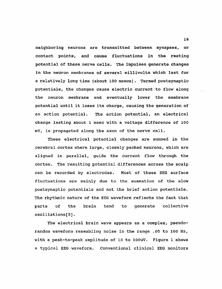
neighboring neurons are transmitted between synapses, or

contact points, and cause fluctuations in the resting

potential of these nerve cells. The impulses generate changes

in the neuron membranes of several millivolts which last for

a relatively long time (about 100 msecs). Termed postsynaptic

potentials, the changes cause electric current to flow along

the neuron membrane and eventually lower the membrane

potential until it loses its charge, causing the generation of

an action potential. The action potential, an electrical

change lasting about 1 msec with a voltage difference of 100

mV, is propagated along the axon of the nerve cell.

These electrical potential changes are summed in the

cerebral cortex where large, closely packed neurons, which are

aligned in parallel, guide the current flow through the

cortex. The resulting potential differences across the scalp

can be recorded by electrodes. Most of these EEG surface

fluctuations are mainly due to the summation of the slow

postsynaptic potentials and not the brief action potentials.

The rhythmic nature of the EEG waveform reflects the fact that

parts of the brain tend to generate collective

oscillations[5].

The electrical brain wave appears as a complex, pseudo

random waveform resembling noise in the range .05 to 100 Hz,

with a peak-to-peak amplitude of 10 to lOOuV. Figure 1 shows

a typical EEG waveform. Conventional clinical EEG monitors

17

EEG Uavefom : S12 point tpooh < 2.0 s > 1

0

-1 500 300 0 100

Points

Figure 1 EEG Waveform

have a frequency response of about 1 to 30 Hz.

Traditionally neurologists have categorized EEG waveforms

as delta, theta, alpha, and beta wave patterns. The

approximate bandwidths of these frequencies are, delta: 0.5 to

4 Hz, theta: 4 to 8 Hz, alpha: 8 to 13 Hz, and beta: above 13

Hz. Beta wave patterns are usually associated with an alert,

awake state of consciousness, and alpha patterns with an

awake, eyes-closed condition. Delta frequencies occur during

deep sleep and in organic brain disease; theta waves occur in

drowsy/sleep conditions and have been correlated with certain

emotional states such as disappointment and frustration[8].

Common anesthetic agents such as ether, enflurane, and

nitrous- oxide produce EEG changes which are similar to the

changes which occur in EEG with loss of consciousness in

sleep. As anesthetic depth increases, the EEG shows slower

activity with waveforms that progressively decrease in

18

frequency and increase in amplitude. A burst-suppression

pattern often occurs in deep anesthesia. This pattern

consists of bursts of high-voltage delta and theta waves,

possibly with intermixed spikes, separated by periods of no

noticeable activity or low-voltage delta/theta waves. At the

deepest levels of anesthesia, there is no EEG electrical

activity.

1.3 EEG TECHNOLOGY

EEG technology has evolved to produce many forms of EEG

recording devices. Compact computer-based EEG analyzers are

the latest introduction; they can display and analyze the EEG

signal from different perspectives by adding computational

capabilities and software extensions to the EEG recorder.

Computerized quantitative EEG analysis is being investigated

for clinical use but is still primarily viewed as an extension

of routine visual inspection[9].

Critical components of the generalized EEG machine

include the input board, input selector switches, calibration

pulses, amplifiers, filters, and the writing or display unit.

The standard EEG machine receives the electrical signal from

scalp electrodes; the input board connects the electrodes to

the input selector switches which select pairs of electrodes

as input to each amplifier in the system. The selector

switches can also select a calibration pulse of known voltage

19

Front Pc

Control* V i d e o Display Umt

EMG Anolog

ADC-board

Video Output

Dual EEG -

ZZZZ I/O bus

CPU - board

E 2 Printer Output

Figure 2 Block Diagram of ABM-2 EEG Monitor

as the input to each recording channel. Differential

amplifiers are used to amplify the voltage difference between

the input electrodes and to reject interference. The

differential amplifiers used have a high voltage gain (usually

about 120 dB) , high input impedance (current designs use above

107 ohms), and high common-mode rejection ratio[3].

The filters in the EEG machine are used to reduce

artifact and preserve the frequency range of interest for the

complex EEG signal. Band pass filters are commonly used; a 60

Hz notch filter is often employed to eliminate power line

interference. The analog EEG signal can be recorded using a

pen writing device and strip chart paper, or on magnetic tape.

Figure 2 shows a block diagram of an EEG'monitor used in this

20

study[10].

1.4 PRELIMINARY ANALYSIS OF THE EEG WAVEFORM

Interpretation of the EEG waveform can be accomplished by

visual inspection, or by automated processing. The first step

in computer analysis is to digitize the EEG waveform at a

minimum of the Nyguist frequency for a short epoch to produce

a finite number of data points. The EEG epoch is usually a

two to 16 second interval[11]. The resulting numerical array

can be treated statistically, using either time or frequency

domain analysis to quantify the information in the EEG.

Time domain analysis uses the original EEG voltage

waveform and calculates such parameters as average signal

amplitude, zero-crossing frequency, and burst suppression

ratio. Signal amplitude can be measured in several ways,

including average peak-to-peak amplitude and RMS amplitude of

the EEG. Zero-crossing analysis involves finding the points

where the EEG tracing crosses the zero-voltage line and

counting the frequency of this occurrence. Burst suppression

analysis measures the proportion of a certain epoch which

represents electrical suppression. The obsolete cerebral

function monitor (CFM) was based on another time-domain

technique. It manipulated a single channel of EEG to produce

an output voltage, termed cerebral function, that was supposed

to vary with changes in EEG; the monitor is no longer used

21

because this mapping proved unreliable[3].

Frequency domain analysis makes use of the spectral

content of the EEG epoch. The technique used is termed power-

spectrum analysis (PSA). Spectral decomposition of the EEG is

performed by computing the Fourier transform of each epoch of

data; this produces the frequency content of the data by

separating the band-limited EEG signal into a finite number of

sine waves whose sum is the original waveform. The EEG signal

is assumed to be a continuous periodic waveform. To estimate

the Fourier transform of a function from a finite number of

sampled points, the discrete Fourier transform of the N points

hk is

N - 1

Hn = E hke2,rjkn/N

k = 0

where n = -N/2, . N/2, belonging in the Nyquist critical

frequency range. hk is calculated by

N - 1

hk = 1/N E Hne-2*jkn/N

n — 0

The Fast Fourier Transform (FFT) is used; it generates a

distinct number of data points based on the epoch of digitized

sample points. The final step in PSA is to calculate the

22

power spectrum for the epoch by squaring and adding the real

and imaginary parts of each of the individual frequency

components. This is based on Parseval's theorem, where the

total power in a signal is

Total power = .„/ | H (f) |2 df

where H(f) is the signal as function of frequency[12]. The

result is a set of frequency bins, expressed in uV2/Hz, each

of which contains the power of the EEG signal at that specific

frequency. Figure 3 shows the power spectrum of the EEG

Sptctral Analysis of EEG ItevefoPM Average FFT of eight tpoohs <312 points each)

P ®'20-l M E 0.15-

8.10 -

0.05 -

25 0 5 10 15 Frequency (HZ>

Figure 3 EEG Power Spectrum

waveform shown in Figure 1.

This data can be used to extract such spectral features

as absolute band powers, median power frequency, spectral edge

frequency, and absolute peak frequency. Absolute band power

23

approximates the area under the spectrum curve between the

upper and lower frequencies of that bandwidth; it is often

calculated for the common delta, theta, alpha, and beta

frequency bands. Median power frequency is defined as the

frequency which bisects the power spectrum. Spectral edge

frequency is that frequency below which a specified

percentage, usually 90 to 95%, of the power in the spectrum

resides. The absolute peak frequency is the frequency that

displays the peak value in a certain epoch or a selected

frequency band.

As an alternative to these statistical distribution

measures for interpretation of the frequency spectrum, the EEG

power spectrum can be displayed in a useful manner. The two

most common real time spectral displays are the compressed

spectral array (CSA) and the density spectral array (DSA).

CSA is a linear display which produces a three-dimensional

graph of frequency versus amplitude versus time. DSA is a

grey-scale display which uses color variations to represent

power at each frequency of an EEG epoch.

1.5 MULTIVARIATE EEG ANALYSIS

Time domain and frequency domain investigative techniques

such as zero-cross detection and spectral analysis are in a

sense primary analytical methods for EEG study[13]. These

strategies produce univariate descriptors of EEG (zero

24

crossing frequency, median frequency, spectral edge frequency,

etc). Multivariate techniques have the capability of

including correlations between several parameters to increase

the information content of the analysis. Multivariate methods

can also be used to perform classification tasks by producing

a single value from many input variables. Artificial Neural

Network (ANN) pattern classification and Discriminant Function

Analysis (DFA) are two of these techniques.

Neural network analysis requires training of the networks

to establish complicated processing patterns which produce an

output value. ANNs have shown promising results in EEG

pattern classification for estimation of anesthetic and

sedation level[14-15]; much research is still needed, however,

to provide an adequate database for ANN training. Research is

also needed to further establish guidelines by which to

determine an optimal combination of the many network factors

such as network architecture, error threshold, momentum, and

learning rate.

DFA, by contrast, is a classical statistical approach

based on a known theoretical framework. This classification

technique is useful for distinguishing patterns containing

many features and dependent variables, where significant

differences among groups can be due to the effect of any

combination of these variables. DFA extracts good-classifying

features by indicating which variables are most important in

25

creating the differences between groups. Information

contained in many independent variables is summarized in a

single index by forming a linear combination of these

independent variables. This linear combination becomes the

basis for assigning classification cases to groups.

DFA derives a function which best discriminates between

groups; its equation is

D = B0 + B,X, + B2X2 + . . . + BpXp

where the X's are the independent variable values and the B's

are the weights, or coefficients estimated from the data.

These weights are chosen so that the between-groups sum of

squares to within-groups sum of squares ratio is a maximum.

This ensures that the values of the discriminant equation are

as different as possible between the groups. Once the

discriminant score is found, a case can be classified into a

group.

The categorizing technique often used is Baye's rule,

where the probability that a classification case with a

discriminant score D belongs to group i is

P (D | Gj) P (Gj)

P (Gj | D) = g

E P (D | Gj) P (G,) i = 1

26

In the equation, P ( G j ) is the a priori probability, or the

likelihood that a case belongs to a group, given no previous

information. This probability can be estimated by several

methods. P(D|Gi) is the conditional probability of D given the

group, and is calculated by assuming the case belongs to a

given group and then estimating the probability of the

resulting discriminant score. P(Gi|D) represents the a

posteriori probability, which is the estimate of how likely it

is that the case belongs to that group.

DFA can be used to select the best variables for group

separation and thus produce good predictor variables. The

stepwise algorithm is a commonly used method for variable

selection. It combines features from two other popular

algorithms, forward entry and backward elimination selection.

The stepwise method considers variables one at a time; it

first considers the best discriminating variable and then adds

the one best variable at a time, until all variables are

entered or until the differentiating power of the discriminant

equation is maximized. Several criteria can be used for

variable selection, including minimization of Wilks' lambda,

Rao's V, and Mahalanobis' distance[16].

DFA can also be used with classification analysis to test

the value of the discriminant function. In this method, the

original scores of the cases used to generate the discriminant

equations are individually plugged back into the function to

27

see if the case's score falls closest to its actual or

predicted group centroid.

28

CHAPTER 2

MATERIALS AND METHODS

2.1 CLINICAL PROTOCOLS

Thirty ASA Physical Status 1 male subjects were included

in this research. These participants were volunteers in a

University of Arizona Medical Center study, approved by the

Human Subjects Committee, to evaluate the effects of the

inhalation anesthetics sevoflurane and enflurane on renal

concentrating ability and cardiovascular and hemodynamic

function. Each subject was included in one of the two

separate protocols for the study.

2.1.1 Protocol One

In the first protocol, 26 subjects were randomly selected

to receive either sevoflurane or enflurane general anesthesia.

Subjects were intravenously induced with propofol and

administered the muscle relaxants succinylcholine and DTC

before intubation. The anesthetic agent, either sevoflurane

or enflurane, was delivered in a mixture of 30-40% oxygen.

The subjects were artificially ventilated at a rate of five to

seven breaths per minute. Fourteen subjects (seven of each

29

anesthetic agent) were maintained at an anesthetic level of 1-

1.2 MAC for a duration of 2.5 to three hours. The remaining

twelve subjects (six sevoflurane and six enflurane) were

maintained at the same 1-1.2 MAC level for eight to 9.6 hours.

Table 1 shows the mean age and weight of the first protocol

subjects in each anesthetic group.

Table 1

Sevoflurane Enflurane

Mean Age 25.4 ± 4.5 yr 26.1 ± 3.7 yr Age Range 21 - 35 yr 22 - 34 yr

Mean Weight 79.2 ± 7.0 kg 73.8 ± 8.4 kg Weight Range 68 - 90 kg 64 - 97 kg

Table 1. Age and Weight of the 26 First Protocol Subjects by Anesthetic

2.1.2 Protocol Two

In the second protocol four subjects received

sevoflurane general anesthesia at varying anesthetic levels.

The subjects were randomly selected to receive the sevoflurane

with one of two background gas mixtures, either 100% oxygen,

or 60% nitrous oxide and 40% oxygen. The subjects were

induced via mask with the anesthetic and 100% oxygen. The

muscle relaxant vecuronium was administered to facilitate

intubation. A transesophageal echocardiograph transducer was

positioned in the esophagus, and a catheter placed in the

30

pulmonary artery for cardiac output measurement. The

anesthetic period included three phases for a total of five to

seven hours of anesthesia.

In the first phase the subjects were artificially

ventilated at a rate of 4-12 breaths per minute and adjusted

to achieve 1.0, 1.5, and 2.0 MAC for 50 minutes at each

anesthetic level. In the second phase the ventilator was set

to allow spontaneous ventilation and the subjects were again

adjusted to the 1.0, 1.5, and 2.0 MAC levels for the 50 minute

periods. In the final phase the subjects were returned to

controlled ventilation and the MAC level varied again. Table

2 shows the mean age and weights for the second protocol

subject group.

Table 2

Mean Age 25.7 ± 3.5 Age Range 22 - 30

Mean Weight 73.2 ± 7.1 Weight Range 68 - 83

Table 2. Age and Weight of the 4 Second Protocol Subjects

2.2 EEG DATA COLLECTION PROTOCOL

After prepping the subject's skin with Nuprep ECG and EEG

skin prepping gel a five-lead set of disposable silver/silver

31

Negative Elsdrods Right

Etoctrode Plaoement

Figure 4

chloride surface electrodes was attached to the frontal and

temporal areas of the forehead. Figure 4 shows a diagram of

the electrode placement. The electrodes were connected

through shielded leads to a brain activity monitor and two

channels, right and left cerebral hemisphere, of EEG waveform

were recorded on FM tape.

Two EEG monitors were used for this study. A Puritan-

Bennett Datex ABM-2 Anesthesia and Brain Activity Monitor was

used for all 2 6 cases of the first protocol; a Neurometries

Lifescan EEG Monitor was employed for the four cases of the

second protocol. The zero to 4.7 volt analog output from the

ABM-2, or the -400 mV to +400 mV analog output from the

Lifescan was connected to a Hewlett Packard 3964A

Instrumentation Recorder calibrated for that voltage range.

32

ABM-2 or Ufescan

* HP 3964A Recorder

Subject EEG Monitor

FM Recorder

Data Collection System

Figure 5

The frequency response of the ABM-2 monitor is 1.5 to 25 Hz

and of the Lifescan is 0.5 to 30 Hz. In all EEG monitors the

specified frequency range attempts to optimize the tradeoff

between artifact and actual signal; most noise at the lower

frequencies is due to motion artifact (electode battery

effect) , and above 25 Hz is due to EMG activity. A block

diagram of the data collection system is shown in Figure 5.

From the recorded EEG waveforms a set number of

contiguous 16 second, 4096-point epochs of EEG was digitized

at 256 Hz for each case. The epochs were chosen by case

documentation and visual inspection to be free of artifact.

The digitization was performed using ASYST software on an IBM-

PC with a Data Translation 2801 12-bit, 16-channel analog-to-

digital converter installed. For each of the 26 cases from

33

the first study protocol ten epochs (five left and five right

hemisphere) were digitized. In addition, for most (9 of 12)

of the nine hour first protocol cases a second set of ten

epochs was recorded and processed; these epochs were taken at

least 5.5 hours later in the anesthesia period than the first

set. For the four cases from the second protocol ten epochs

(five left and five right) were recorded and digitized for

each anesthetic level/ventilation mode combination. The ASYST

digitization source code is included in Appendix A.

2.3 PRIMARY ANALYSIS OF EEG DATA

All EEG left and right channel data were treated

separately. Power-spectrum analysis was performed, as the FFT

average spectral signature of each 4096-point epoch was

calculated and stored as a 64-point array. This was done in

two steps; the FFT and power spectrum was computed using ASYST

software (included in Appendix A). The resulting 256-point

spectral content arrays were then further processed, using

software written in C, to produce the average spectral

signature 64-point arrays. Each component of these arrays

corresponds to 0.5 Hz, with a DC to 32 Hz frequency range

included.

C software (included in Appendix B) was then used to

extract eight parameters. From the digitized raw waveform

34

files RMS amplitude and zero-crossing frequency (measured in

crossings/sec) were calculated. From the power spectrum files

EEG spectral signatures, consisting of average power in each

of four frequency bands (0-4 Hz, 4-8 Hz, 8-13 Hz, and 13-25

Hz) as a percent of total spectral power, were calculated.

Median frequency and spectral edge frequency (defined to be

the frequency below which 95% of the power in the spectrum

resides) were also computed. InStat statistical package

software was used to compare the eight parameters for

differences between anesthetics, duration of anesthetic

period, and anesthetic MAC level using Student's t-tests. For

reference, cardiovascular variables (heart rate, and systolic

and diastolic blood pressure) measured during the sample time

of the EEG recorded epoch were also compared for statistical

significance between the different anesthetic conditions.

2.4 DISCRIMINANT FUNCTION ANALYSIS

Discriminant Function Analysis of the 64-point EEG

spectral signatures was performed using SPSS software

statistical package. For the 26 subjects from the first study

protocol the analysis was done to classify the cases according

to anesthetic agent. DFA was also used on the 12 nine-hour

first protocol cases to classify the early-in-case (within the

second hour of the anesthesia period) spectral signature

35

versus the late-in-case (within the eighth hour of anesthesia)

signature; these were done separately for sevoflurane and

enflurane cases. The DFA was performed on the second study

protocol cases to classify each spectral signature according

to MAC level, done separately for controlled ventilation and

spontaneous ventilation phases.

For all instances, the DFA procedure was the same.

Initially all the data sets for that analysis run (for

example, the 2 6 spectral signatures for the anesthetic-type

classification) were used to calculate the discriminant

function weighting coefficients when the case type was known.

The predictability of the function was then tested by the

"leave-one-out" method, where all but one of the data sets are

used to calculate new weighting coefficients and the remaining

case (introduced as unknown case type) is classified using the

new coefficients.

The single case is classified as belonging to the group

whose centroid is closest to the discriminant score for that

case. By plugging the original variables of the left-out case

back into the new discriminant function, the reliability of

the initial function is tested, and an indication of

correlation among cases with like type is produced. This

predictability evaluation was done once for each of that

analysis-run's number of data sets, so that each case was

excluded and tested once.

In order to select the best variables, or EEG

frequencies, for group separation the stepwise analysis method

was then used. The minimization of Wilk's lambda variable

selection criterium was used to generate a set of the best

discriminating frequencies for group classification. Lambda

is a measure of the power of the already selected variables,

defined as the ratio of within-groups sum-of-squares to total

sum-of-squares. The number of steps allowed (related to

variables considered for inclusion) in the stepwise analysis

was set to the SPSS maximum; this is the maximum possible

without creating a loop in which a variable is repeatedly

cycled in and out[17]. This then generated a maximum,

variable by analysis-run, number of best-predictor

frequencies. For consistency in right/left EEG data

comparison, the number of frequencies included in the final

set of best variables was taken to be the smaller of the two

right/left groups.

The classifying ability of this set of significant

frequencies was then tested by again using the leave-one-out

method. The same procedure described above, excluding and

testing each case once, was used; this time the data set for

each case was made up of only the set of best predictor

frequencies. Subsets of these significant frequencies were

also tested to determine whether a subgroup could provide a

more accurate predictor. The theory being tested in this

37

frequency subset analysis was that perhaps some of the

frequencies in the 64-point EEG spectral signatures provide no

information, or possibly cloud the discriminant analysis.

38

CHAPTER 3

RESULTS : PROTOCOL ONE CASES

3.1 UNIVARIATE STATISTICAL RESULTS

3.1.1 Anesthetic Group Differences

Student's t-tests found statistically significant

differences (p < 0.05) between the anesthetics sevoflurane and

enflurane in several of the EEG parameters. Differences in

spectral edge frequency and average power in both the 4-8 Hz

frequency band and the 13-25 Hz frequency band were especially

significant, with a two-tailed p value of < .0001. Results

from the t-tests are summarized in Table 3. RMS amplitude,

and the delta and alpha frequency power were not significantly

different between anesthetics. Figures 6-9 are graphs of

the average data values for the statistically significant EEG

parameters.

Of the reference cardiovascular variables, measured

during the sample time of the EEG recorded epochs, only

diastolic blood pressure showed a difference between the two

anesthetic groups. It showed marginal significance (p < .09)

with a slightly higher diastolic blood pressure for the

sevoflurane cases than the enflurane cases.

39

Table 3

Sevoflurane Enflurane (top: right EEG (top: right EEG bottom: left) bottom: left)

Average 40.8 ± 7.9% 43.9 ± 12.2% P < .4587 power 0-4 Hz 44.9 ± 9.0% 44.7 ± 13.1% P < .9587

Average 29.3 ± 3.7% 19.5 ± 4.8% P < .0001** power 4-8 Hz 29.9 ± 3.4% 19.7 ± 4.5% P < .0001**

Average 24.1 ± 8.4% 28.0 ± 11.8% P < . 3486 power 8-13 Hz 21.2 ± 8.5% 27.9 ± 13 .7% P < . 1489

Average 5.2 ± 3 .2% 8.6 ± 2 .2% P < .0043** power 13-25 Hz 3.9 ± 1 . 3% 7.6 ± 2 .2% P < .0001**

Spectral 12.8 ± 1.8 HZ 15.0 ± 1.2 Hz P < .0017** edge freq. 12.1 ± 1.0 Hz 14.4 ± 1.4 Hz P < .0001**

Median 4.8 ± 8 .4 Hz 5.6 ± 2 .1 Hz P < .2078 freq.

4.4 ± 0 .8 HZ 5.6 ± 2 .4 HZ P < . 09*

Zero 7.1 ± 1 . 0 7.8 ± 1 . 1 P < . 09* cross freq. 6.9 ± 0 .8 7.9 ± 1 . 1 P < .0174**

RMS 0.15 ± . 03 0.14 ± .03 P < .5378 amplit.

0.15 ± . 05 0.14 ± .03 P < . 6209

** significant * marginally significant

Table 3. Summary Data from First Protocol Cases (26 total) showing differences in EEG parameters between anesthetics. Units of zero-cross freq. are crossings per sec, of RMS amplitude are scaled volts.

Average Power 4-8 Hz Band All Protocol 1 Cases (26 total)

35-

30-

(•

« 15-

Subject Case Number

ESS Sevoflurane (Right) 00 Enflurane (Right) KS Sevoflurane (Left) Bnflurane (Left)

Figure 6

Average Power 13-25 H2 Band All Protocol 1 Caees (26 total)

1 2 3 4 5 6 7 8 9 10 11 12 13

Subject Case Number

ESS Sevoflurane (Right) Bnflurane (Right) ES Sevoflurane (Left) Bnflurane (Left)

Figure 7

Average Spectral Edge Frequency All Protocol 1 Coses (26 total)

s h 0) Cn T3 W

17-

16-

15-

14-

13-

12-

1 1 - V •

D

*

P

D

•fr

•

Subject Case Number

Sevoflursne (Right) ^ Bnflurane (Right) Sevoflurane (Left) • Bnflur&ne (Left)

Figure 8

J2 U O 0* 0)

11

10-

C •H CO to 0 u V

>1 u e G) O1 0) M

0 u I 0 0) N

9-

8 -

7-

• +

Average Zero-crossing Frequency All Protocol 1 Cases (26 total)

V

* *

9 4 * A

+

• • * *

R *

—i 1 r~

1 2 3 4 5 6 7 8 9 10 11 12 13 Subject Case Number

Sevoflurane (Right) -+• Bnflurane (Right) *C Sevoflurane (Left) Q Bnflurane (Left)

Figure 9

42

3.1.2 Differences Between Duration of Anesthetic Period

Paired t-tests were used to determine differences between

duration of anesthetic period, since the change in anesthetic

condition was intra-subject. Significant differences were

found between the early-in-case and late-in-case EEG

parameters for the sevoflurane subject group but not for the

enflurane subjects. In the right channel EEG data, power in

the 4-8 Hz and 13-25 Hz bands, zero-crossing frequency, and

spectral edge frequency showed the lowest p values for the t-

tests. Median frequency and average power in the 0-4 Hz band

showed no significant differences. Table 4 summarizes the t-

test results for significantly different EEG parameters

between length of anesthetic phase (sevoflurane subjects

only).

Data for the most significantly different of these EEG

parameters are graphed in Figures 10 - 13. The cardiovascular

variable heart rate showed a marginally significant difference

(p < .07) between length of anesthesia for the sevoflurane

subjects only. Average heart rate was higher for the late-in-

case period than for early period.

Table 4

43

Early in case Late in case (top: right EEG (top: right EEG bottom: left) bottom: left)



Average 22.8 ± 5.4% 29.4 ± 10.6% P < .06* power 8-13 Hz 21.4 ± 7.6% 27.4 ± 0.1% P < .1983

Average 3.7 ± 0.9% 6.5 ± 0 .6% P < .0035** power 13-25 Hz 3.5 ± 1.4% 5.9 ± 2 .7% P < .0413**

Spectral 11.9 ± 0.9 Hz 14.0 ± 0.3 Hz P < .0016** edge freq. 12.0 ± 0.5 Hz 13.9 ± 1.4 HZ P < .0517*

Median 4.6 ± 0.6 HZ 5.6 ± 1 .9 HZ P < . 1656 freq.

4.4 ± 0.6 Hz 5.3 ± 2 .3 HZ P < .3853

RMS 0.14 ± .02 0.13 ± . 02 P < .0194** amplit.

0.13 ± .04 0.12 ± .04 P < .1042

Zero 6.7 ± 0.7 8.1 ± 0 .7 P < .0033** cross freq. 6.7 ± 0.6 8.3 ± 1 .2 P < .0264**


Table 4. Summary Data from Sevoflurane 9-hour Cases (5 total) showing significant differences in EEG parameters between duration of anesthesia. Units of RMS amplitude are scaled volts. Units of zero-cross frequency are in crossings/sec.

Sevo Cases Average Power 4-8 Hz Band Protocol 1 9-hour Cases (5 total)

I

Subject Case Number

| Early (Right BEG) | | Late (Right BBG) KS Barly (Left BBG) fTTTI Late (Left BBG)

Figure 10

Sevo Cases Average Power 13-25 Hz Band Protocol 1 9-hour Cases (5 total)

Subject Case Number

Boa Barly (Right BBG) HI Late <Ri9ht BBG) L.W Early (Left BBG) j^Q] Late (Left BBG)

Figure 11

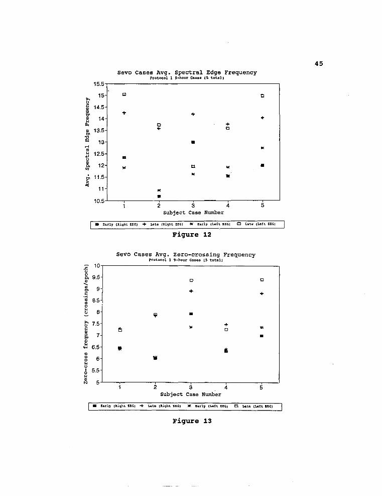
15.5-

u c 0) & 0) 14 b 0) Cn TJ W

CO M •P U SL l/J

tJ> £

10.5

Sevo Cases Avg. Protocol 1

Spectral Edge 9-hour Cases (5 total]

Frequency

a a

+ +

D •4-+ D

•

B

* a W. • * n

m m

2 3 4 Subject Case Number

Early (Right EEC) Ute (Right BEG) * Early (Left BBG) • Late (Left BBG)

Figure 12

Sevo Cases Avg. Zero-crossing Frequency Protocol 1 9-hour Cases (5 total)

X 0 o a Q>

G •H o (0 O o

>1 u c a) & 0) u

10-

9.5- Q •

9- +

8.5 J

8- •

7.5-s £ *

7- •

6.5- * i

6- ik

5.5-

1 2 3 4 Subject Case Number

5

• Early (Right BBG) •+ Late (Right BBG) W. BarLy (Left BBG) • Late (Left BBG)

Figure 13

3.2 DISCRIMINANT ANALYSIS RESULTS

46


The leave-one-out classification method correctly

classified 69.3% of the right EEG channel data and 76.9% of

the left channel data cases according to anesthetic group when

the full 64-point spectral signatures were used. When the set

of best discriminating frequencies, determined by the stepwise

analysis method, was used these percentages were notably

improved. Table 5 shows the most significant frequencies for

discriminating between anesthetic agents, determined by the

stepwise method for the 26 protocol one cases. Table 6

summarizes the classification results using the 64-point

spectral signatures and also the subsets of frequencies.

47

Table 5

Freq Spectral Actual Frequency Wilk's lambda # Array point Bin

R 1 9 4 - 4.5 HZ .602 I 2 6 2.5 - 3 HZ .356 G 3 61 30 - 30.5 Hz .290 H 4 22 10.5 - 11 HZ .154 T 5 60 29.5 - 30 Hz .130

6 26 12.5 - 13 HZ .111 E 7 18 8.5 - 9. HZ .083 E 8 34 16.5 - 17 Hz .077 G 9* 64 31.5 - 32 Hz .068

L 1 31 15 - 15.5 Hz .694 E 2 63 31 - 31.5 Hz .392 F 3 20 9.5 - 10 Hz . 347 T 4 34 16.5 - 17 Hz .287

5 32 15.5 - 16 Hz .255 E 6 56 27.5 - 28 Hz .239 E 7 50 24.5 - 25 Hz .216 G 8 22 10.5 - 11 Hz .200

9 30 14.5 - 15 Hz .177

* 15 significant frequencies were found for right EEG data by stepwise method

Table 5. Most Significant Nine Frequencies For Discriminating Between Anesthetics Determined by Stepwise Method Using All 26 Protocol One Cases

48

Table 6

Sevoflurane cases

(top: right EEG bottom: left)

Enflurane cases


Total cases


64 pt spect. sign.

69.2%

84.6%

69.2%

69.2%

69.2%

76.9%

top 9 freqs

92.3%

92.3%

100%

92.3%

96.1%

92.3%

top 6 freqs

92.3%

100%

100%

84.6%

96.1%

92.3%

top 84.6% 92.3% 88.5% 3 freqs 100% 76.9% 88.5%

Table 6. Percentage of Correctly Classified Cases By Anesthetic Type for Each subgroup, using All frequencies and Subsets

49

3.2.2 Differences Between Duration of Anesthetic Period

The leave-one-out method of case classification was done

separately for the two anesthetic groups. For sevoflurane

cases analysis with the full 64-point spectral signature

correctly categorized 90% of the right data sets and 88.9% of

the left data sets according to length of anesthesia. The

right EEG data showed perfect classification with the set of

significant frequencies, but left EEG data classification was

not improved with the stepwise significant frequencies.

In enflurane cases, 50% accurate right data results and

87.5% correct left results were obtained using all

frequencies. Both right and left results were improved with

the significant frequencies as input. Tables 7 and 8 display

the stepwise significant frequencies for sevoflurane and

enflurane groups respectively. Tables 9 and 10 show the

classification results for each anesthetic group.

50

Table 7


R 1 10 4.5 - 5 HZ .315 I 2 8 3.5 - 4 Hz .118 G 3 33 16 - 16.5 Hz .081 H 4 49 24 - 24.5 Hz .027 T 5 11 5 - 5.5 Hz .014

6* 45 22 - 22.5 Hz .005

1 2 0.5 - 1 Hz .669 L 2 6 2.5 - 3 Hz .303 E 3 4 1.5 - 2 Hz .135 F 4 24 11.5 - 12 Hz .032 T 5 23 11 - 11.5 Hz .015

6 10 4.5 - 5 Hz .007

* 7 significant frequencies were found for right EEG data by stepwise method

Table 7. Most Significant Six Frequencies For Discriminating Between Duration of Anesthesia Period Determined by Stepwise Method Using 9-hour Sevoflurane Cases (5 total)

Table 8


R 1 25 12 - 12.5 Hz .245 I 2 9 4 - 4.5 HZ . 114 G 3 39 19 - 19.5 HZ .041 H 4 37 18 - 18.5 Hz .007 T 5 21 10 - 10.5 Hz .002

L 1 64 31.5 - 32 Hz .481 E 2 14 6.5 - 7 Hz .114 F 3 2 0.5 - 1 Hz .045 T 4 49 24 - 24.5 Hz .004

5 3 1 - 1.5 Hz .001

Table 8. Most Significant Five Frequencies For Discriminating Between Duration of Anesthesia Period Determined by Stepwise Method Using 9-hour Enflurane Cases (4 total)

51

Table 9

Early in case

Late in case

Both sets




64 80% pt spect. 80% sign.

100%

100%

90%

88.9%

top 100% 6 freqs 80%

100%

75%

100%

77.8%

top 100% 100% 100%

freqs 80% 100% 88.9%

top 100% 100% 100%

freqs 80% 100% 88.9%

Table 9. Percentage of Correctly Classified Cases By Duration of Anesthetic Period for Sevoflurane 9-hour cases (5 total)

52

Table 10

Early in case

Late in case

Both sets




64 pt spect. sign.

50%

75%

50%

100%

50%

87.5%

top 5 freqs

100%

100%

100%

100%

100%

100%

top 100% 100% 100%

freqs 100% 100% 100%

top 75% 100% 87.5%

freqs 100% 100% 100%

Table 10. Percentage of Correctly Classified Cases By Duration of Anesthetic Period for Enflurane 9-hour cases (4 total)

53

CHAPTER 4

RESULTS : PROTOCOL TWO CASES

4.1 UNIVARIATE STATISTICAL RESULTS

Paired t-tests for significant differences in EEG

parameters between anesthetic levels were done separately for

the two ventilation mode phases of data. In the controlled

ventilation phase spectral edge frequency showed significant

difference between the 1.0 and 1.5 MAC level, and marginal

significance between 1.5 and 2.0 MAC. Zero-crossing frequency

and power in the 8-13 Hz band showed marginal significance

between the lightest and deepest MAC levels; the other EEG

parameters showed no statistically significant differences.

The reference cardiovascular variables all showed significance

between MAC levels. Tables 11 and 12 summarize the t-test

results for the EEG parameters and Table 13 for the

cardiovascular variables. Figures 14 - 15 graph the average

data for spectral edge frequency.

For the spontaneous ventilation phase, power in the 4-8

Hz band, and power in the 8-13 Hz band showed significant

differences between MAC levels. Spectral edge frequency and

zero-crossing frequency showed marginal significance, and the

54

other EEG parameters were not statistically different. None

of the cardiovascular variables were significantly different

between anesthetic levels. Results of the t-tests for this

ventilation phase data are summarized in Tables 14 and 15.

Figures 16 through 18 graph the average data for the most

significant EEG parameters. Burst suppression was observed at

anesthetic concentrations above 1.5 MAC during both

ventilation modes in two of the subjects.

Table 11

55

1.0 to 1.5 MAC

1.0 MAC 1.5 MAC (top: right EEG (top: right EEG bottom: left) bottom: left)





RMS 0.26 ± .07 0.30 ± .04 P < .3313 amplit.

0.27 ± .07 0.32 ± .05 P < .2652

Median 1.9 ± 0.1 Hz 2.2 ± 0.9 Hz P < .5428 freq.

2.0 ± 0.2 Hz 2.2 ± 0.8 Hz P < .5688

Spectral 12.0 ± 1.5 HZ 10.5 ± 1.4 HZ P < .0008** edge freq. 11.9 ± 1.6 Hz 10.3 ± 1.3 Hz P < .0059**

Zero 5.7 ± 0.8 5.3 ± 1.3 P < .2700 cross freq. 5.6 ± 0.8 5.1 ± 1.1 P < .1049


Table 11. Summary Data from Controlled ventilation phase showing significant differences in EEG parameters between 1.0 and 1.5 MAC levels. Units of zero-cross frequency are crossings/sec, of RMS amplit. are scaled volts.

56

Table 12

1.5 to 2.0 MAC






RMS 0.30 ± .04 0.28 ± .06 P < .5934 amplit.

0.32 ± .04 0.29 ± .06 P < .4552

Median 2.2 ± 0.9 Hz 2.1 ± 0.3 HZ P < .7679 freq.

2.2 ± 0.8 Hz 2.1 ± 0.2 HZ P < .8397

Spectral 10.5 ± 1.4 Hz 9.0 ± 0.5 Hz P < .0807* edge freq. 10.3 ± 1.3 Hz 9.0 ± 0.3 HZ P < .0919*



Table 12. Summary Data from Controlled ventilation phase showing significant differences in EEG parameters between 1.5 and 2.0 MAC levels. Units of zero-cross frequency are crossings/sec, of RMS amplit. are scaled volts.

57

Table 13

1.0 to 1.5 MAC

1.0 MAC 1.5 MAC

Systolic 102.7 ±8.4 92.5±8.9 p< .0440** blood pr.

Diastol. 57.3 ± 6.3 52.7±4.7 p< .0511* blood pr.

Heart 63.3 ± 9.9 71.3 ± 10.5 p < .0280** rate

1.5'to 2.0 MAC

1.5 MAC 2.0 MAC

Systolic 92.5 ± 8.9 85.1 ± 10.3 p < .0362** blood pr.

Diastol. 52.7 ± 4.7 50.8 ± 7.2 p < .2532 blood pr.

Heart 71.3 ± 10.5 78.7 + 10.3 p < .0001** rate


Table 13. Summary Data from Controlled ventilation phase showing significant differences in cardiovascular parameters between MAC levels. Units for blood pressures are in mm Hg, for heart rate is beats/min.

Avg. Spectral Edge Freq. (1.0-1.5 MAC) Protocol 2 Cams Controlled Vent.

cr 13

2 3

Subject Case Number

1.0 MAC (Right) + 1.5 MAC (Right) * 1.0 MAC (Uft) • 1.5 MAC (L«£t)

Figure 14

Avg. Spectral Edge Freq. (1.0-2.0 MAC) Protocol 2 Cases Controlled Vent.

>n 14

?r 13

2 3

Subject Case Number

1.0 HAC (Right) •+• 3.0 MAC (Right) *C 1.0 MAC (L«ft) C3 3.0 MAC (Loft)

Figure 15

Table 14

59

1.0 to 1.5 MAC






RMS 0.25 ± .14 0.22 ± .06 P < .7288 amplit.

0.26 ± .15 0.22 ± .06 P < .6252

Median 4.9 ± 5.4 Hz 3.7 ± 1.0 Hz P < .6540 freq.

4.3 ± 4.3 Hz 3.6 ± 0.8 Hz P < .7477

Spectral 13.0 ± 6.4 Hz 13.3 ± 2.4 HZ P < .9125 edge freq. 12.4 ± 6.2 Hz 13.1 ± 2.3 Hz P < .7884



Table 14. Summary Data from Spontaneous ventilation phase showing significant differences in EEG parameters between 1.0 and 1.5 MAC levels. Units of zero-cross frequency are crossings/sec, of RMS amplt. are scaled volts.

Table 15

60

1.5 to 2.0 MAC



Average 18.5 ± 5.5% 21.4 ± 5.7% P < .0757* power 4-8 Hz 19.0 ± 5.0% 21.3 ± 6.0% P < .1310

Average 21.3 ± 6.8% 12.0 ± 11.1% P < .1434 power 8-13 Hz 21.2 ± 5.4% 11.2 ± 10.1% P < . 1154

Average 5.8 ± 4.1% 2.2 ± 0.5% P < . 1453 power 13-25 Hz 5.6 ± 3.9% 2.0 ± 0.4% P < .1361

RMS 0.22 ± .06 0.25 ± .05 P < .3847 amplit.

0.22 ± .06 0.26 ± .04 P < .3637

Median 3.7 ± 1.0 HZ 3.2 ± 0.9 HZ P < .3202 freq.

3.6 ± 0.8 Hz 3.1 ± 0.8 Hz P < .2457

Spectral 13.3 ± 2.4 Hz 9.5 ± 0.6 Hz P < .08* edge freq. 13.1 ± 2.3 Hz 9.2 ± 0.8 HZ P < .08*

Zero 7.5 ± 1.2 5.5 ± 0.9 P < .1083 cross freq. 7.4 ± 1.0 5.3 ± 0.6 P < .06*


Table 15. Summary Data from Spontaneous ventilation phase showing significant differences in EEG parameters between 1.5 and 2.0 MAC levels. Units of zero-cross frequency are crossings/sec, of RMS amplt. are scaled volts.

Average Power 4-8 Hz Band (1.0-1.5 MAC) Protocol 2 Cases Spontaneous Vent.

2 3 Subject Case Number

IRS8S 1.° HAC (Right) BB 1.5 HAC (Right) ̂ 1.0 KAC (Left) |_|_U 1.5 MAC (Left)

Figure 16

Average Power 4-8 Hz Band (1.0-2.0 MAC) Protocol 2 Cases Spontaneous Vent.

2 3 Subject Case Number

S5S 1.0 KAC (Right) I | 2.0 HAC (Right) ESi .o KAC (Left) rm 2.0 KAC (Left)

Figure 17

Average Power 8-13 Hz Band (1-1.5 MAC) Protocol 2 Cases Spontaneous Vent.

Subject Case Number

l^g 1.0 MAC (Right) BH !-5 MAC (Right) ^ 1.0 MAC (Left) ITTI 1.5 MAC (Left)

Figure 18

63

4.2 DISCRIMINANT ANALYSIS RESULTS

DFA leave-one-out case classification was done separately

for the two ventilation mode EEG data sets. For the

controlled ventilation mode data, 75% of the right EEG data

and 41.7% of the left channel data were correctly categorized

by MAC level when the full 64-point spectral signature was

used. These percentages were improved when the stepwise

significant frequencies were used for discrimination.

In spontaneous ventilation mode data, analysis with the

full frequency spectrum accurately classified 25% of the right

data and 58.3% of the left data. Dramatic improvement in

these percentages was shown with the set of best-predictor

frequencies. Tables 16 and 17 present the significant

frequencies for controlled and spontaneous ventilation phase

EEG data. Tables 18 and 19 summarize the classification

results for these two data sets.

64

Table 16


R 1 21 10 - 10.5 HZ .634 I 2 8 3.5 - 4 HZ .219 G 3 42 20.5 - 21 Hz .047 H 4 15 7 - 7.5 Hz .017 T 5 2 0.5 - 1 Hz .006

6 17 8 - 8.5 Hz . 002 E 7 10 4.5 - 5 Hz . 0004 E 8 48 23.5 - 24 Hz .00008 G

L 1 21 10 - 10.5 Hz .600 E 2 8 3.5 - 4 Hz . 221 F 3 44 21.5 - 22 Hz . 068 T 4 50 24.5 - 25 Hz .035

5 16 7.5 - 8 Hz . 009 E 6 15 7 - 7.5 Hz .001 E 7 55 27 - 27.5 Hz . 0004 G 8 54 26.5 - 27 Hz .00008

Table 16. Most Significant Eight Frequencies For Discriminating Between MAC Levels Determined by Stepwise Method Using Controlled Ventilation Phase Data

65

Table 17


R 1 41 20 - 20.5 Hz .415 I 2 6 2.5 - 3 Hz . 161 G 3 26 12.5 - 13 Hz . 036 H 4 27 13.5 - 14 Hz . 015 T 5 40 19.5 - 20 Hz .007

6 21 10 - 10.5 Hz .002 7 11 5 - 5.5 Hz .0002

L 1 49 19.5 - 20 Hz .352 E 2 36 17.5 - 18 Hz . 079 F 3 27 13 - 13.5 Hz . 030 T 4 18 8.5 - 9 Hz . 009

5 28 13.5 - 14 Hz . 002 6 25 12 - 12.5 Hz . 001 7* 21 10 - 10.5 Hz . 0001

* Eight significant frequencies were found for left EEG data by stepwise method

Table 17. Most Significant Seven Frequencies For Discriminating Between MAC Levels Determined by Stepwise Method Using Spontaneous Ventilation Phase Data

66

Table 18

1.0 MAC 1.5 MAC 2.0 MAC All Data data data data sets

sign.

(top: right EEG data, bottom: left EEG)

64 75% 75% 75% 75% pt spect. 50% 25% 50% 41.73

top 75% 75% 100% 83.33 8 freqs 100% 100% 100% 100%

top 75% 75% 100% 83.3% 6 freqs 100% 100% 100% 100%

top 75% 75% 100% 83.33 3 freqs 75% 50% 75% 66.7%

Table 18. Percentage of Correctly Classified Cases By Anesthetic Level for Controlled Ventilation Phase Data

67

Table 19

1.0 MAC 1.5 MAC 2.0 MAC All Data data data data sets

(top: right EEG data, bottom: left EEG)

64 50% 0% 25% 25% pt spect. 100% 25% 50% 58.3% sign.

top 100% 100% 75% 91.7% 7 freqs 100% 100% 100% 100%

top 100% 100% 100% 100% 5 freqs 100% 100% 100% 100%

top 75% 100% 100% 91.7% 3 freqs 75% 75% 100% 83.3%

Table 19. Percentage of Correctly Classified Cases By Anesthetic Level for Spontaneous Ventilation Phase Data

68

CHAPTERS

DISCUSSION

5.1 PROTOCOL ONE CASES


The EEG spectral signatures of the sevoflurane and

enflurane subject groups differed significantly, indicating

that the two anesthetics have dissimilar effects on the human

EEG. The mean percent power in the low range of the frequency

spectrum was significantly higher in the sevoflurane subjects

than in the enflurane subjects. This was evidenced by the

sevoflurane subjects showing significantly lower spectral edge

frequency, lower median frequency, less average power in the

13-25 Hz band, and more average power in the 4-8 Hz band than

the enflurane subjects. Interpretation of these EEG changes

is complex and difficult[5] . It would seem safe to state that

enflurane anesthesia results in higher frequency cerebral

activity than sevoflurane anesthesia; perhaps this is

consistent with the fact that patients under enflurane

anesthesia sometimes exhibit EEG pattern seizure activity[1].

It is also possible that the difference in EEG spectral

signatures for the two anesthetic groups is due to a

69

fallacious assumption concerning the anesthetic depth level of

the subjects. It was assumed that the subjects in both groups

were at the same anesthetic depth level, since they were being

maintained at one MAC as determined by the anesthesiologist.

As was mentioned in the first chapter, MAC is only a

statistical predictor of depth, not an actual individual

measure of anesthetic depth. Perhaps the concentration

values, determined by prior research and used by the

anesthesiologist to determine the 1.0 MAC level, were

incorrect. This could result in the sevoflurane subjects

actually being at a different, possibly deeper, level of

anesthesia than the enflurane subjects.

Despite a fair amount of inter-subject diversity in

spectral signatures for each anesthetic subject group, DFA

produced a high percentage of correct case classification by

anesthetic agent when the best-predictor frequencies were

used. Categorization results using the full 64-point spectral

signatures were not as accurate, indicating the value of the

stepwise generation of significant frequencies technique.

Subsets of these best-predictor variables performed well also.

An interesting comparison between the t-test

statistically different (between anesthetics) power bands and

the frequencies selected as best-discriminating variables by

DFA was made. T-tests showed the theta and beta power bins to

be significant, and a majority (67%) of the DFA significant

70

frequencies belonged to those two frequency ranges.

5.1.2 Differences Between Duration of Anesthesia

Only the sevoflurane subjects showed significant

differences between duration of anesthetic period; the small

number of cases (5 subjects) made statistical significance

difficult to prove. Even so, the EEG recorded early in the

anesthetic period for these subjects showed significantly

lower spectral edge frequency, less average power in the 4-8

Hz range, and more average power in the 8-25 Hz range than the

EEG recorded at least 5.5 hours later. This indicates a

progressive increase in high frequency cerebral activity with

increased duration of 1.0 MAC sevoflurane anesthesia. Heart

rate also showed a slightly higher average value with longer

anesthetic period.

The increases in both cardiovascular and EEG activity

with increased duration of anesthesia for the sevoflurane

subjects suggests that these physiologic systems were able to

"bounce back", or stabilize from the effects of the anesthetic

over time. In the beginning stages of the anesthetic period

heart rate and EEG activity were depressed by the effect of

the anesthetic, but activity gradually increased with

prolonged anesthesia. This effect was not evident in the

enflurane subjects, perhaps indicating that the effects of

71

sevoflurane are more easily adjusted for by the body than

those of enflurane.

DFA also showed differences between length of anesthesia.

A high percentage of correct classifications by time in case

was made for the sevoflurane subjects; this percentage was

improved for right EEG data using the set of significant

frequencies, but not for left channel data.

DFA could correctly categorize 100% of the enflurane

cases by anesthetic duration using the best-predictor

frequencies. Since the t-tests did not show significant

differences between anesthetic length in EEG parameters for

the enflurane subjects, this would suggest that DFA can detect

subtle EEG differences more readily than standard univariate

statistics. The small number of these enflurane cases (4

subjects) is also a factor.

Rather surprisingly a subset of only the top two

significant frequencies provided better classification results

than when the full spectral signatures were used. This

supports the theory that many of the frequencies in the 64-

point EEG spectral signature provide no, or confusing,

information.

5.2 PROTOCOL TWO CASES

Changes with respect to anesthetic level in the EEG

72

spectral signatures for these subjects were consistent with

the literature for both the controlled and spontaneous

ventilation phases of the anesthetic period. Despite the

small number of cases (4), EEG recorded at lighter MAC levels

showed significantly less mean percent power in the lower

frequency ranges than EEG from deeper MAC levels.

Average percent power in the 8-13 Hz band showed

different trends for the two different ventilation phases:

there was more alpha activity at the 1.0 MAC level than for

deeper anesthetic concentrations during controlled

ventilation, and the reverse was true during spontaneous

ventilation. The reason for this is unclear, but is probably

related to end tidal C02 levels. During the spontaneous

ventilation phase the subjects have the added CNS stress of

increased C02 levels (a natural result of cessation of

artificial ventilation) which probably acts as a stimulus and

effectively reduces anesthetic depth. Cardiovascular

variables changes as expected with anesthetic level; again,

the relation to EEG is unclear.

In both ventilation phases the significantly different

EEG parameters demonstrated more changes between the first MAC

level increase (1.0 to 1.5 MAC) than the next increase,

suggesting threshold levels.

Despite considerable inter-subject spectral signature

diversity, DFA again correctly classified a high percentage of

73

EEG data cases by anesthetic level when the best-predictor

frequencies were used for discrimination. With such a small

number of cases, comparison between univariate statistics

(classification of anesthetic level by spectral edge

frequency) and DFA is difficult.

74

CHAPTER 6

CONCLUSIONS

Both the analytical techniques, univariate parametric

statistics and DFA, showed significant differences in EEG data

between anesthetic agents, duration of anesthetic period, and

anesthetic MAC level. of the set of eight standard EEG

parameters investigated, spectral edge frequency and percent

power in the 4-8 Hz and 13-25 Hz bands were the most valuable

for distinguishing between overall anesthetic conditions. The

0-4 Hz power bin, median frequency, and RMS amplitude

parameters held the least information for this study.

The DFA stepwise method of determining best-predictor

frequencies proved very accurate for classifying EEG data

according to anesthetic conditions. A possible concern is

raised involving the DFA methodology used when inspecting the

significant frequencies for the first protocol subjects. A

few of the best-predictor frequencies are of such high

frequency (above the frequency range of the EEG monitor used

for these cases) that they are suspect of being artifact or

noise. The full 64-point spectral signature range,

corresponding to DC to 32 Hz, should probably have been

75

reduced for these subjects.

Considerable inter-subject diversity in EEG spectral

signatures was observed. This confirms the difficulty of EEG

interpretation, and the need for more research and a larger

database. Typically, clinical studies are conducted using

small numbers of subjects; therefore the data collected in

this researach represents an important contribution to

clinical EEG understanding. The data collected for this

research is especially valuable since opportunities to observe

the effects of anesthetics on EEG during the ideal conditions

present for this clinical study (no surgery to cause motion

artifact, healthy subjects) are very rare.

76

CHAPTER 7

FUTURE WORK

A future study should include a larger population size

for the varied anesthetic level part of this research. In-

depth Neural Network Analysis of all the EEG data collected

for this project, already partially completed by Mr. Rich

Watt, may also yield useful findings. As mentioned in the

previous section, greater care should be taken to reduce

artifact in the data by reducing the spectral signature array

to match the frequency response of the EEG monitor being used.

Since considerable intra-subject variation in right and

left channel EEG was observed, it would be interesting to note

whether subjects are right or left-handed and include these

correlations in future research.

APPENDIX A

ASYST SOURCE CODE

ASYST DIGITIZATION CODE

79

\ EEG-S.PRG

\ this program performs digitization of analog input \ thanks to Dr. M. Navabi who wrote the majority of this code DEF.VUPORT FORGET.ALL

\ A-D board used is Data Translation 2801 DT2800 20 STRING FILENAME INTEGER DIM[ 4 096 , 2 ] ARRAY BUFFER.1 buffer INTEGER DIM[ 4096 , 2 ] ARRAY BUFFER.2 buffer REAL DIM[ 08500 ] ARRAY L.BUFFER.T REAL DIM[ 08500 ] ARRAY L.BUFFER.B INTEGER SCALAR EXIT.FLAG

SCALAR SAVE.FLAG SCALAR RATE SCALAR C SCALAR COUNT SCALAR L.COUNT SCALAR S.COUNT SCALAR OFFSET SCALAR SECONDS

\ Set up first data

\ Set up second data

\ Maximum size 11250

REAL

0 1 A/D.TEMPLATE FORE/BACK buffering 2 A/D.GAIN input range

BUFFER.1 BUFFER.2 DOUBLE.TEMPLATE.BUFFERS

CYCLIC at beginning

\ Set up a template for double

\ Set up for -2.5 to 2.5 volts

\ 2 a/d.gain ==> for 0 to 2.5

\ Assign the 2 buffers

\ If buffer is full, start filling other buffer

: SET.TASK.RATE INV 1000. *

(ms) DUP 53. / DUP 1 MODULO - 1 +

# 1 DUP 1 TASK.MODULO / TASK.PERIOD

/

\ [ Sample rate (Hz) — ] \ sample rate into time

\ Save it \ #times to cycle thru task

\ before doing task \ time between samplings

INIT.ACQ \ [ Sample rate (Hz) — ] FORE/BACK \ Set current template .2 CONVERSION.DELAY \ and delay between channel

80

samples A/D.INIT \ Init template

CLEAR.TASKS 1 TASK A/D.IN>ARRAY

using FORE/BACK

\ Clear task table \ task 1 is A/D to array

SET.TASK.RATE \ Set up task modulo and period

PRIME.TASKS \ Prepare tasks

VUPORT TOP VUPORT CENTER VUPORT BOTTOM VUPORT FULL

: SETUP.GRAPHICS GRAPHICS.DISPLAY \ Set up graphics TOP 0. .6 VUPORT.ORIG 1. .4 VUPORT.SIZE VUPORT.CLEAR OUTLINE BOTTOM 0. .2 VUPORT.ORIG 1. .4 VUPORT.SIZE VUPORT.CLEAR OUTLINE TOP AXIS.DEFAULTS VERTICAL AXIS.FIT.OFF GRID.OFF HORIZONTAL AXIS.FIT.OFF GRID.OFF NORMAL.COORDS 0.08 0.08 AXIS.ORIG 0.08 0.08 AXIS.POINT 0.88 0.88 AXIS.SIZE 8 8 AXIS.DIVISIONS HORIZONTAL 0 2 LABEL.POINTS LABEL.SCALE.OFF VERTICAL 0 4096 WORLD.SET HORIZONTAL 0 4096 WORLD.SET \ set h-axis for 4096 points VERTICAL 2 2 LABEL.POINTS VERTICAL -1. 0 5 LABEL.FORMAT 0.02 0.01 TICK.SIZE 0 0 TICK.JUST LABEL.SCALE.OFF XY.AXIS.PLOT L.BUFFER.T LINE.BUFFER.ON

81

BOTTOM AXIS.DEFAULTS VERTICAL AXIS.FIT.OFF GRID.OFF HORIZONTAL AXIS.FIT.OFF GRID.OFF NORMAL.COORDS 0.08 0.08 AXIS.ORIG 0.08 0.08 AXIS.POINT 0.88 0.88 AXIS.SIZE 10 10 AXIS.DIVISIONS HORIZONTAL 0 2 LABEL.POINTS LABEL.SCALE.OFF VERTICAL 0 4096 WORLD.SET HORIZONTAL 0 4096 WORLD.SET VERTICAL 2 2 LABEL.POINTS VERTICAL -1. 0 5 LABEL.FORMAT 0.02 0.01 TICK.SIZE 0 0 TICK.JUST LABEL.SCALE.OFF XY.AXIS.PLOT L.BUFFER.B LINE.BUFFER.ON

: PLOT.DATA 20 3 GOTO.XY ." TOP ERASE.LINES LINE.BUFFER.CLEAR VERTICAL 0 4 096 WORLD.SET HORIZONTAL 0 256 WORLD.SET

points DUP XSECT[ 1 ] sub[ 1 , 256 ,

ii

\ plot 1 out of every 16

16 ] 12 COLOR Y.DATA.PLOT

BOTTOM ERASE.LINES LINE.BUFFER.CLEAR VERTICAL 0 4 096 WORLD.SET HORIZONTAL 0 256 WORLD.SET \ plot 1 out of every 16

points XSECT[ 2 ] sub[ 1 , 256 , 16 ] 14 COLOR Y.DATA.PLOT

\ HORIZONTAL 0 102 4 WORLD.SET \ DUP XSECT[ 1 ] 2048 - FFT ZMAG \ DUP SUB[ 2 , 1024 , 1 ] []MAX 1.2 * DUP 60 1 goto.xy . \ VERTICAL 0 swap WORLD.SET \ ERASE.LINES \ LINE.BUFFER.CLEAR \ 12 COLOR SUB[ 2 , 1024 , 1 ] Y.DATA.PLOT \ XSECT[ 2 ] 2048 - FFT ZMAG \ 14 COLOR SUB[ 2 , 1024 , 1 ] Y.DATA.PLOT 4 096. RATE / SECONDS + SECONDS := 60 2 GOTO.XY SECONDS .

82

20 3 GOTO. XY .11 PRESS 'Q' TO QUIT

SETUP.FILE FILE.TEMPLATE END ." ENTER TWO DIGIT SUBJECT NUMBER, (e.g. 04):" "INPUT " E2_" "SWAP "CAT " .DAT" "CAT FILENAME ":= FILENAME DEFER> FILE.CREATE FILENAME DEFER> FILE.OPEN

\ digitize at specified input sampling rate : ACQ&PLOT \ [ Sample rate (Hz) — ]

DUP RATE := SETUP.FILE SETUP.GRAPHICS 0 EXIT.FLAG := 0 SAVE.FLAG := 0 SECONDS := INIT.ACQ \ Initialize for acq TRIGGER.TASKS \ Go

BEGIN \ Acquire until 'Q' is pressed

BEGIN ?key IF

key DUP 81 = 113 = OR IF 1 EXIT.FLAG := ELSE 1 SAVE.FLAG := THEN

THEN SAVE.FLAG 1 =

IF STACK.CLEAR ?BUFFER.A/B IF BUFFER.1 ELSE BUFFER.2 THEN APPEND.ARRAY>FILE 0 SAVE.FLAG :=

then 7BUFFER.SWITCH \ Loop around until array

is full UNTIL 7BUFFER.A/B \ Which array was filled? IF

BUFFER.1 ELSE

BUFFER.2

83

THEN

PLOT.DATA \ Plot the last filled array

1 EXIT.FLAG = UNTIL STOP.TASKS \ Done with background acq FILE.CLOSE

\ The following program will sample channels 0 and 1 of the A/D \ board with a sampling rate which should be put on the stack \ prior to calling the program. This program is different from \ ACQ&PLOT in that it stores automatically into a file with \ extension '.TMP'. The '.TMP' file should be converted to a \ '.DAT' file using a different subroutine.

: ACQ&STORE \ [ Sample rate (Hz) — ] DUP RATE := SETUP.FILE SETUP.GRAPHICS 0 EXIT.FLAG := 0 SAVE.FLAG := 0 SECONDS := INIT.ACQ \ Initialize for acq TRIGGER.TASKS \ Go

BEGIN \ Acquire until ' Q ' is pressed

BEGIN ?key IF

key DUP 81 = 113 = OR IF 1 EXIT.FLAG := THEN

THEN 7BUFFER.SWITCH \ Loop around until array

is full UNTIL ?BUFFER.A/B \ Which array was filled? IF

BUFFER.1 ELSE

BUFFER.2 THEN PLOT.DATA \ Plot the last filled

array SECONDS 16 / C := 16 17 18 24 25 26 31 32 33 39 40 41 54 55 56 89 90 91

84

121 122 123 128 129 130 139 140 141 C = C = C = C = C = C = C = C = C = C = C = C = C = C = C = C = C = C = C = C = C = C = C = C = C = C = C = OR OR OR OR OR OR OR OR OR OR OR OR OR OR OR OR OR OR OR OR OR OR OR OR OR OR IF

1 SAVE.FLAG := 20 3 GOTO.XY AUTOSAVING

THEN SAVE.FLAG 1 = IF

STACK.CLEAR 7BUFFER.A/B IF BUFFER.1 ELSE BUFFER.2 THEN APPEND.ARRAY>FILE 0 SAVE.FLAG :=

THEN 153 C = IF

1 EXIT.FLAG := THEN

1 EXIT.FLAG = UNTIL STOP.TASKS \ Done with background acq FILE.CLOSE

: CHOOSE ENTER TWO DIGIT SUBJECT NUMBER, (e.g. 04):"

"INPUT " E2_" "SWAP "CAT FILENAME ":= FILE.TEMPLATE END FILENAME " .DAT" "CAT DEFER> FILE.CREATE

GRAPHICS.DISPLAY \ Set up graphics TOP 0. .73 VUPORT.ORIG 1. .27 VUPORT.SIZE VUPORT.CLEAR CENTER 0. .46 VUPORT.ORIG 1. .27 VUPORT.SIZE VUPORT.CLEAR

85

BOTTOM 0. .19 VUPORT.ORIG 1. .27 VUPORT.SIZE VUPORT.CLEAR FULL 0. .2 VUPORT.ORIG 1. .8 VUPORT.SIZE

FILENAME " .TMP" "CAT DEFER> FILE.OPEN FILE.CONTENTS SWAP DROP DUP L.COUNT := 1 - COUNT := FILE.CLOSE BEGIN

FILENAME " .TMP" "CAT DEFER> FILE.OPEN L.COUNT COUNT - SUBFILE BUFFER.1 FILE>ARRAY

1 ] TOP 12 BUFFER.1 XSECT[ BUFFER.1 XSECT[ L.COUNT COUNT -BUFFER.1 XSECT[ BUFFER.1 XSECT[ L.COUNT COUNT -BUFFER.1 XSECT[ BUFFER.1 XSECT[ SCREEN.CLEAR 1 4 GOTO.XY ."

FOR COMBINATION) " #INPUT CASE 1 OF L.COUNT COUNT - SUBFILE BUFFER.1 FILE>ARRAY ENDOF 2 OF L.COUNT COUNT - 1 + SUBFILE BUFFER.1 FILE>ARRAY ENDOF 3 OF L.COUNT COUNT - 2 + SUBFILE BUFFER.1 FILE>ARRAY ENDOF 4 OF

2 4 GOTO.XY 1&2; 2 FOR 2&3) "

#INPUT DUP

COLOR Y.AUTO.PLOT 2 ] 14 COLOR Y.DATA.PLOT 1 + SUBFILE BUFFER.1 FILE>ARRAY 1 ] CENTER 12 COLOR Y.AUTO.PLOT 2 ] 14 COLOR Y.DATA.PLOT 2 + SUBFILE BUFFER.1 FILE>ARRAY 1 ] BOTTOM 12 COLOR Y.AUTO.PLOT 2 ] 14 COLOR Y.DATA.PLOT

WHICH BUFFER DO YOU WANT? (1, 2, 3, OR 4

" WHICH COMBINATION DO YOU WANT? ( 1 FOR

1 =

2 =

2 4

SUBFILE BUFFER.1 FILE>ARRAY 1 + SUBFILE BUFFER.2 FILE>ARRAY

IF L.COUNT COUNT L.COUNT COUNT

THEN IF L.COUNT COUNT

L.COUNT COUNT THEN GOTO.XY ." ENTER THE OFFSET IN THE FIRST ARRAY?

1 + 2 +

SUBFILE BUFFER.1 FILE>ARRAY SUBFILE BUFFER.2 FILE>ARRAY

#INPUT OFFSET BUFFER.1 SUB [ BUFFER.1 SUB[ BUFFER.2 SUB[ BUFFER.1 SUB[

OFFSET , 4096 OFFSET -1 , 4096 OFFSET - , 1 ; 1 , OFFSET , 1 ; ! ] 4 096 OFFSET - , OFFSET

i ; i ]

] : =

86

ENDOF ENDCASE FULL BUFFER.1 XSECT[ 1 ] 12 COLOR Y.AUTO.PLOT BUFFER.1 XSECT[ 2 ] 14 COLOR Y.DATA.PLOT FILE.CLOSE 2 4 GOTO. XY ." DO YOU WANT TO STORE THIS BUFFER? (

l=STORE, 0=REDO ) " #INPUT DUP 1 = IF

FILENAME " .DAT" "CAT DEFER> FILE.OPEN BUFFER.1 APPEND.ARRAY>FILE FILE.CLOSE COUNT 3 - COUNT :=

THEN COUNT 0 = UNTIL

: CHOOSE.512 ." ENTER TWO DIGIT SUBJECT NUMBER, (e.g. 04):" "INPUT " E2_" "SWAP "CAT FILENAME ":= FILE.TEMPLATE END FILENAME " .DAT" "CAT DEFER> FILE.CREATE

GRAPHICS.DISPLAY \ Set up graphics TOP 0. .73 VUPORT.ORIG 1. .27 VUPORT.SIZE VUPORT.CLEAR CENTER 0. .46 VUPORT.ORIG 1. .27 VUPORT.SIZE VUPORT.CLEAR BOTTOM 0. .19 VUPORT.ORIG 1. .27 VUPORT.SIZE VUPORT.CLEAR FULL 0. .2 VUPORT.ORIG 1. .8 VUPORT.SIZE

FILENAME " .TMP" "CAT DEFER> FILE.OPEN FILE.CONTENTS SWAP DROP DUP L.COUNT := 1 - COUNT := FILE.CLOSE BEGIN

87

FILENAME " .TMP" "CAT DEFER> FILE.OPEN L.COUNT COUNT - SUBFILE BUFFER.1 FILE>ARRAY BUFFER.1 XSECT[ 1 ] TOP 12 COLOR Y.AUTO.PLOT BUFFER.1 XSECT[ 2 ] 14 COLOR Y.DATA.PLOT L.COUNT COUNT - 1 + SUBFILE BUFFER.1 FILE>ARRAY BUFFER.1 XSECT[ 1 ] CENTER 12 COLOR Y.AUTO.PLOT BUFFER.1 XSECT[ 2 ] 14 COLOR Y.DATA.PLOT L.COUNT COUNT - 2 + SUBFILE BUFFER.1 FILE>ARRAY BUFFER.1 XSECT[ 1 ] BOTTOM 12 COLOR Y.AUTO.PLOT BUFFER.1 XSECT[ 2 ] 14 COLOR Y.DATA.PLOT SCREEN.CLEAR 1 4 GOTO. XY . " YOU MUST SELECT 8 SUB-BUFFERS OF 512 POINTS

EACH. " PCKEY DROP ?DROP FULL \ FULL-SCREEN VUPORT 0 S.COUNT := 4 1 DO

L.COUNT COUNT - I + 1 - SUBFILE BUFFER.2 FILE>ARRAY 9 1 DO

VUPORT.CLEAR BUFFER.2 SUB[ I 512 * 511 - , 512 , 1 ; ! ] DUP DUP

\ AXIS.DEFAULTS \ VERTICAL 0 4 096 WORLD.SET \ HORIZONTAL 0 512 WORLD.SET \ XY.AXIS.PLOT

XSECT[ 1 ] 12 COLOR Y.AUTO.PLOT XSECT[ 2 ] 14 COLOR Y.DATA.PLOT 12 FOREGROUND 70 1 GOTO.XY I . 15 FOREGROUND 1 3 GOTO.XY ." SO FAR YOU HAVE SELECTED: " S.COUNT . 1 4 GOTO.XY ." DO YOU WANT THIS SUB-BUFFER? (1=YES ,

0=NO) " #INPUT SCREEN.CLEAR 1 = IF

BUFFER.1 SUB[ S.COUNT 512 * 1 + , 512 , 1 ; ! ] := S.COUNT 1 + S.COUNT :=

ELSE DROP

THEN LOOP

LOOP BUFFER.1 XSECT[ 1 ] 12 COLOR Y.AUTO.PLOT BUFFER.1 XSECT[ 2 ] 14 COLOR Y.DATA.PLOT FILE.CLOSE 1 4 GOTO.XY . " DO YOU WANT TO STORE THIS BUFFER? (

l=STORE, 0=REDO ) " #INPUT DUP 1 = IF

88

FILENAME " .DAT" "CAT DEFER> FILE.OPEN BUFFER.1 APPEND.ARRAY>FILE FILE.CLOSE COUNT 3 - COUNT : =

THEN COUNT 0 = UNTIL

ASYST FFT CODE

90

\ FFT-S.PRG

\ this program does the fft of the 4096 point input files, and \ stores the result as a 256 point array representing the \ power spectrum \ Thanks again to Dr. Navabi DEF.VUPORT FORGET.ALL 20 STRING FILENAME INTEGER DIM[ 4096 , 2 ] ARRAY BUFFER.1 \ Set up data buffer REAL DIM[ 4096 ] ARRAY BUFFER

DIM[ 512 ] ARRAY FFT.BUFFER VUPORT TOP VUPORT BOTTOM

: SETUP.GRAPHICS GRAPHICS.DISPLAY \ Set up graphics TOP 0. .6 VUPORT.ORIG 1. .4 VUPORT.SIZE VUPORT.CLEAR OUTLINE BOTTOM 0. .2 VUPORT.ORIG 1. .4 VUPORT.SIZE VUPORT.CLEAR OUTLINE TOP AXIS.DEFAULTS VERTICAL AXIS.FIT.OFF GRID.OFF HORIZONTAL AXIS.FIT.OFF GRID.OFF NORMAL.COORDS 0.08 0.08 AXIS.ORIG 0.08 0.08 AXIS.POINT 0.88 0.88 AXIS.SIZE 8 8 AXIS.DIVISIONS HORIZONTAL 0 2 LABEL.POINTS LABEL.SCALE.OFF VERTICAL 0 4096 WORLD.SET HORIZONTAL 0 4096 WORLD.SET \ set h-axis for 4096 points VERTICAL 2 2 LABEL.POINTS VERTICAL -1. 0 5 LABEL.FORMAT 0.02 0.01 TICK.SIZE 0 0 TICK.JUST LABEL.SCALE.OFF XY.AXIS.PLOT BOTTOM AXIS.DEFAULTS VERTICAL AXIS.FIT.OFF GRID.OFF

91

HORIZONTAL AXIS.FIT.OFF GRID.OFF NORMAL.COORDS 0.08 0.08 AXIS.ORIG 0.08 0.08 AXIS.POINT 0.88 0.88 AXIS.SIZE 10 10 AXIS.DIVISIONS HORIZONTAL 0 2 LABEL.POINTS LABEL.SCALE.OFF VERTICAL 0 4096 WORLD.SET HORIZONTAL 0 4096 WORLD.SET VERTICAL 2 2 LABEL.POINTS VERTICAL -1. 0 5 LABEL.FORMAT 0.02 0.01 TICK.SIZE 0 0 TICK.JUST LABEL.SCALE.OFF XY.AXIS.PLOT

: PLOT.DATA 20 3 GOTO.XY ." TOP ERASE.LINES VERTICAL 0 4096 WORLD.SET HORIZONTAL 0 256 WORLD.SET

points DUP XSECT[ 1 ] sub[ 1 , 256 ,

ii

\ plot 1 out of every 16

16 ] 12 COLOR Y.DATA.PLOT

BOTTOM ERASE.LINES VERTICAL 0 4 096 WORLD.SET HORIZONTAL 0 256 WORLD.SET \ plot 1 out of every 16

points DUP XSECT[2 ] sub[ 1 , 256 , 16 ] 14 COLOR Y.DATA.PLOT HORIZONTAL 0 1024 WORLD.SET DUP XSECT[ 1 ] 2 048 - FFT ZMAG dup sub[ 2 , 1024 , 1 ] []max 1.2 * DUP 60 1 goto.xy . VERTICAL 0 swap WORLD.SET ERASE.LINES 12 COLOR SUB[ 2 , 1024 , 1 ] Y.DATA.PLOT XSECT[ 2 ] 2048 - FFT ZMAG 14 COLOR SUB[ 2 , 102 4 , 1 ] Y.DATA.PLOT

: GET.FILE.NAME ." ENTER TWO DIGIT SUBJECT NUMBER, (e.g. 21):" "INPUT " E2_" "SWAP "CAT FILENAME ":=

7

\ store as ascii 256 point array

92

: DISP&STORE.FFT 47 I + ASCII" "CAT " .DAT" "CAT DEFER> OUT>FILE 257 1 DO

FFT.BUFFER [ I ] DUP * . CR \ STORE AS POWER SPECTRUM LOOP OUT>FILE.CLOSE

7

\ do fft 512 points at a time : FFT.512 BUFFER 2048.0 / DUP 4096.0 / []SUM - BUFFER := BUFFER SUB[ 1 , 512 , 1 ] FFT ZMAG BUFFER SUB[ 512 , 512 , 1 ] FFT ZMAG + BUFFER SUB[ 1024 , 512 , 1 ] FFT ZMAG + BUFFER SUB[ 1024 512 + , 512 , 1 ] FFT ZMAG + BUFFER SUB[ 2 048 , 512 , 1 ] FFT ZMAG + BUFFER SUB[ 2048 512 + , 512 , 1 ] FFT ZMAG + BUFFER SUB[ 3072 , 512 , 1 ] FFT ZMAG + BUFFER SUB[ 3072 512 + , 512 , 1 ] FFT ZMAG + DUP FFT.BUFFER := SUB[ 1 , 256 , 1 ] Y.AUTO.PLOT 7

: DO.FFT GET.FILE.NAME SETUP.GRAPHICS FILENAME " .DAT" "CAT DEFER> FILE.OPEN FILE.CONTENTS SWAP DROP FILE.CLOSE -14 7 SCI.FORMAT 1 + 1 DO

FILENAME " .DAT" "CAT DEFER> FILE.OPEN I SUBFILE BUFFER.1 FILE>ARRAY FILE.CLOSE

\ left channel output file BUFFER.1 XSECT[ 1 ] BUFFER := FFT.512 FILENAME 11 LF" "CAT TOP DISP&STORE.FFT

\ right channel output file BUFFER.1 XSECT[ 2 ]

BUFFER := FFT.512 FILENAME " RF" "CAT BOTTOM DISP&STORE.FFT

20 3 GOTO.XY ." SUBFILE #" LOOP

APPENDIX B

C SOURCE CODE

95

C STATISTICAL ANALYSIS CODE

96

/* Stats.c */ /* 8-20-92 */

#include <stdio.h> #include <math.h> #include <string.h>

/* A.A. Gale */ /* This program performs the standard statistical analysis on the raw & fft

EEG data files. For raw data files : It calculates two standardized parameters : integrated amplitude and zero crossing frequency. Each data file

represents one 16 second epoch of right or left EEG data. For fft data files : It calculates 6 params : delta, theta, alpha, & beta power

bins, and median and spectral edge frequency. Program also creates avg. 64-point spectral signature

files. */

main()

FILE *fp, *fo; FILE *fa_r, *fa_l; char line[81]; char f_name[50], fo_name[50], name[50], fft_name[50]; char av_namel[50], av_namer[50]; int i; int s_done, m_done; /* flags */ float z_cross; /* zero crossing frequency */ int num_points; float value; float temp; double squared_amp, sum_squares; double variance; double rms_value; /* rms amplitude */ double t_power, m_power, s_power; double last_sum; double f_increment, d_ratio, diffl, diff2; double mn_freq, spec_freq; /* median &

spec, edge frequency */ double delta, theta, alpha, beta; /* frequency bins */

double zsum_r, zsuiti_l, ampsum_r, ampsum_l, dsum_r, dsum_l double tsum_r, tsum_l, asum_r, asum_l, bsum_r, bsum_l; double msum_r, msum_l, ssum_r, ssum_l; double avg_l[64], avg_r[64]; int g;

/* initialize everything */ zsum_r=0.0; zsum_l=0.0; ampsum_r=0.0; ampsum_l=0.0

dsum_r=0.0; dsum_l=0.0; tsum_r=0.0; tsum_l=0.0; asum_r=0.0; asum_l=0.o; bsum_r=0.o

bsum_l=0.0; msum__ir =0.0; msum_l =0.0'; ssum_r =0.0; ssum_l = 0.0;

/* initialize avg. arrays */ for (i = 0; i < 64; i++) {

avg_l[i] = 0.0; avg_r[i] = 0.0;

}

/* open raw data file and process */ printf ("Please enter input data file number, eg: 15A .\n") gets(line); sscanf(line,"%s" , name);

strcpy(fo_name,name) ; streat(fo_name/'.out") ; strcpy(av_namer, name); strcat(av_namer, ".rav"); strcpy(av_namel, name); strcat(av_namel, ".lav");

if ( ((fo = f open (fo_name, "w")) == NULL) |j ((fa_r fopen(av_namer, "w"))

== NULL) |] ((fa_l = fopen(av_namel, "w")) == NULL) ) {

printf("Can't open output files ", "%s", fo_name, "\n") exit(l);

}

for(g = 0; g < 10; g++) { /* initialization */ t_power = 0.0; sum_squares = 0.0; z_cross = 0.0; mn_freq = spec_freq = 0.0; num_points = 4 096;

strcpy(f_name, ""); strcpy(fft_name, "");

switch(g)

/* {

Set up files names for the 5 continuous epochs

case 0 : strcpy strcpy strcat strcat strcat strcat break;

case 1 : strcpy strcpy strcat strcat

strcat strcat break;






f_name, "e2"); fft_name, "e2"); fft_name, name); fft_name, "rfO.dat"); f_name, name); f name, "rOO.dat");

f_name, "e2"); fft_name, "e2"); fft_name, name); fft_name, "rfl.dat");

f_name, name); f_name, "rOl.dat");

f_name, "e2"); fft_name, "e2"); fft_name, name); fft_name, "rf2.dat");

f_name, name); f_name, "r02.dat");

f_name, "e2"); fft_name, "e2"); fft_name, name); fft_name, "rf3.dat");

f_name, f name,

name); "r03.dat");

f_name, "e2"); fft_name, Me2"); fft_name, name); fft_name, "rf4.dat");

strcat(f name, name);

strcat(f name, break;

case 5 : strcpy f_name, strcpy fft_name strcat fft_name strcat fft_name

strcat f_name, strcat f_name, break;



case 7 : strcpy f name, strcpy fft_name strcat fft_name strcat fft_name

strcat f name, strcat f_name, break;

case 8 : strcpy f name, strcpy fft name strcat fft_name strcat fft_name




•100.

"e2");

"e2"); name); "If2.dat"

"103.dat");

"104.dat");

} /* end switch */

if ((fp = fopen(f_name, "r")) == NULL) {

printf("Can't open input file ", "%s", f_name, "\n") exit(1);

} else {

/* Loop through and process raw data files */ for(i = 0; i < num_points; i++) {

fgets(line, 81, fp); line[strlen(line) - 1] = '\0'; sscanf(line, "%e"f Svalue);

/* calculate zero crossing frequency */ /* this is calculated in one direction only */ if (i > 0) { if ((temp >= 0) && (value < 0))

{ z_cross++;

} } temp = value;

/* calculate RMS amplitude */ squared_amp = value * value; sum_squares = sum_squares + squared_amp;

> /* end for */

/* calculate zero cross per second — 16 second epochs z_cross = z_cross/16.0;

/* calculate rms amplitude */ variance = sum_squares / num_points; rms_value = sqrt(variance); if (g < 5) {

zsum_r = zsum_r + z_cross; ampsum_r = ampsum_r + rms_value;

} else {

zsum_l = zsum_l + z_cross; ampsum_l = ampsum_l + rms_value;

101

}

fprintf(fo,"\n\n"); fprintf(fo,"%s%s%s%f\n", "Zero crossing frequency for ",

f_name, " is : z_cross);

fprintf(fo,"%s%lf\n", "RMS amplitude is : rms_value);

fclose(fp); } /* end else */

/* open and process fft files */

/* cut frequency range of interest to 0 to 32 Hz since this describes EEG range — thus only look at 64 points of

the 256 point fft files */

num_points = 64 ;

if ((fp= fopen(fft_name, "r")) == NULL) {

printf("Can't open file ", '^s", f_name, "\n"); exit(1);

} else { for (i = 0; i < num_points; i++) {

fgets(line, 81, fp); line[strlen(line) - 1] = '\0'; sscanf(line, "%e", &value); if (g < 5) avg_r[i] += value;

else avg_l[i] += value;

/* calculate total power in epoch */ /* Envelope approximation used is square-edge method */ /* 0.5 is the half-Hertz frequency increments */

t_power = t_power + (0.5 * value);

/* calculate power in the four frequency bins */ /* Delta is < 4 Hz Theta is 4 to < 8 Hz Alpha is 8 to 13 Hz Beta is > 13 Hz

102

7 /* frequency is 3.5 Hz */ if (i == 7)

delta = t_power; if (i == 15) /* frequency is 7.5 Hz */

theta = t_power - delta; if (i == 25) /* frequency is 12.5 Hz */

alpha = t_power - (delta + theta);

} /* end for */ beta = t_power - (delta + theta + alpha); /* all

frequencys above 13 Hz */

/* m_power is the 50% power location */ m_power =0.5 * t_power;

/* s_power is the 95% power location */ s_power = 0.95 * t_power;

fclose(fp);

/* calculate power in bins as percentage of total power */ delta = delta / t_power; theta = theta / t_power; alpha = alpha / t_power; beta = beta / t_power;

if (g < 5) {

dsum_r += tsum_r += asum_r += bsum_r +=

} else {

dsum_l += tsum_l += asum_l += bsum_l +=

}

delta; theta; alpha; beta ;

delta; theta; alpha; beta;

fprintf(fo,"%s%f\n","Delta power percentage is ",delta);

fprintf(fo,"%s%f\n","Theta power percentage is ",theta);

fprintf(fo,"%s%f\n","Alpha power percentage is alpha);

fprintf(fo,"%s%f\n","Beta power percentage is : ",beta);

103

/* reopen fft file to loop thru data again */

fp= fopen(fft_name, "r");

s_done =0; /* zero the found 95% flag */ m_done = 0; /* zero the found 50% flag */

t_power = 0.0;

for(i =0; i < num_points; i++) {

if (s_done) break; fgets(line, 81, fp); line[strlen(line) - 1] = '\0'; sscanf(line, "%e", &value);

last_sum = t_power; t_power = t_power + (0.5 * value);

/* calculate median frequency */ if (!m_done) { if (t_power >= m_power) {

m_done = 1; if (t_power - m_power) { /* 0.5 Hertz intervals */

mn_freq = (i + 1) * 0.5; } else {

diffl = t_power - last_sum; diff2 = m_power - last_sum; d_ratio = diff2 / diffl;

/* increment from lower frequency is 0.5 Hertz x d_ratio

f_increment = d_ratio * 0.5; mn_freq = (i * 0.5) + f_increment; if (g < 5) {

msum_r += mn_freq; } else {

msum_l += mn_freq; }

104

} } /* end if t_power >= etc */ } /* end if !m_done */

/* calculate spectral edge frequency */ if (t_power >- s_power) { s_done =1; if (t_power == m_power) { /* 0.5 Hertz intervals */

spec_freq = (i + 1) * 0.5; } else {

diffl = t_power - last_sum; diff2 = s_power - last_sum; d_ratio = diff2 / diffl;

/* increment from lower frequency is 0.5 Hertz x d_ratio */

f_increment = d_ratio * 0.5; spec_freq = (i * 0.5) + f_increment; if (g < 5) {

ssum_r += spec_freq; } else {

ssum_l += spec_freq; }

} } /* end if t_power >= etc */

} /* end for */

fclose(fp); } /* end else */

fprintf(fo,"%s%f\n","Median frequency is : ",mn_freq); fprintf(fo,"%s%f\n","Spectral Edge frequency is :

",spec_freq);

} /* end big for */

/* calculate average stats */ zsum_r = zsum_r / 5.0; zsum_l /= 5.0; ampsum_r /= 5.0; ampsum_l /= 5.0; dsum_r /= 5.0; dsum_l /= 5.0;

tsum_r /= 5.0; tsum_l /= 5.0; asum_r /= 5.0; asum_l /= 5.0; bsum_r /= 5.0; bsum_l /= 5.0; msum_r /= 5.0; msum_l /= 5.0; ssum_r /= 5.0; ssum_l /= 5.0;

/* write avg. fprintf(fo, fprintf(fo, fprintf(fo, fprintf(fo, fprintf(fo, fprintf(fo, fprintf(fo, fprintf(fo,

stats to file */ "%f%s%f\n", zsum_r, " "%f%s%f\n", ampsum_r, "%f%s%f\n", dsum_r, "%f%s%f\nM, tsum_r, "%f%s%f\n", asum_r, "%f%s%f\n", bsum_r, "%f%s%f\n", msum_r, "%f%s%f\n", ssum_r,

/* create avg for (i =0; i < {

avg_r[i] /= 5 . avg_l[i] /= 5

fprintf(fa_r, fprintf(fa_l,

}

fclose(fa_r); fclose(fa_l); fclose(fo); exit(0); /* end main */

power spectrum 64; i++)

0 ; 0 ; "%f\n", "%f\n",

avg_r[i]) ; avg_l[i]);

, zsum_l); 11, ampsum_l)

, dsum_l); , tsum_l); , asum_l); , bsum_l); , msum_l); , ssum_l);

files */

C PROGRAM TO PREP DATA FOR INPUT TO SPSS DISCRIMINANT ANALYSIS

107

/* discrim.c for 5 cases */ /* 10-21-92 */

/* A.A. Gale */ /* This program preps the average fft data files for input to the SPSS program Discriminant analysis run. Data files are set up so that each file has one number per line. Data are in this order : 64 frequency bins, case type (manually added to files later by me), case number. Data files are separate for left and right eeg. */

#include <stdio.h> #include <math.h> #include <string.h>

main()

FILE *fp, *fo; FILE *fa_r, *fa_l; char line[81]; char linel[81]; char av_namel[50], av_namer[50]; int i, g, case_num; float value, val;

if (((fo = fopen("dislr.dat", "w")) == NULL) jj ((fp = f o p e n ( " d i s l l . d a t " , " w " ) )

== NULL) ) {

printf("Can't open output files ", "\n"); exit(1);

}

for(g = 0; g < 5; g++) {

strcpy(av_namel, ""); strcpy(av_namer, ""); switch(g) {

case 0 : strcpy(av_namel, "01.lav"); strcpy(av_namer, "Ol.rav"); break;

case 1 :

108

strcpy(av_namel, "02.lav"); strcpy(av_namer, "02.rav"); break;

case 2 : strcpy(av_namel, "03.lav"); strcpy(av_namer, "03.rav"); break;



} /* end switch */

if (((fa_r = fopen(av_namer, "r")) == NULL) || ((fa_l = fopen(av_namel, "r")) == NULL))

{ printf("Can't open input file \n") ; exit(1) ;

} else {

for(i = 0; i < 64; i++) {

fgets(line, 81, fa_r); linefstrlen(line) - 1] = '\0'; sscanf(line, "%e", Svalue); fgets(linel, 81, fa_l); linel[strlen(linel) - 1] = '\0'; sscanf(linel, "%e", &val);

fprintf(fo,"%f\n", value); fprintf(fp,"%f\n", val); } case_num = g + 1;

fprintf(fo, "%d\n", case_num); fprintf(fp, "%d\n", case_num);

} /* end else */ fclose(fa_r); fclose(fa_l);

• /* end big for */

fclose(fo); fclose(fp); /* end main

APPENDIX C

SPSS PROCEDURES

Ill

S P S S P r o c e d u r e f o r s t e p w i s e m e t h o d :

DATA LIST PILE 'file.flat' FREE / freql to freq64 drug case.

DSCRIMINANT /GROUPS drug (1,2) /VARIABLES freql to freq64 /METHOD WILKS.

Notes : file.dat is the input data file. freql to freq64 are the first 64 #'s in the file, next 2 numbers are the drug type and case #.

All 64 freq's are used in the stepwise method.

SPSS Procedure for leave-one-out classification :

DATA LIST FILE 'file.dat' FREE / freql to freq64 drug case.

DSCRIMINANT /GROUPS drug (1,2) /VARIABLES freql to freq64 /STATISTICS 1 2 10 13 14 15 16.

Notes : The data file, file.dat, is modified for each run of this procedure. For each run, the "drug" entry is changed to be a dummy value (anything outside the 1 -2 range of the drug variable) for the one subject case to be left out for that run.

Variables can either be the full 64-point set of freq's, or can be the subset of significant freq's which came from the stepwise method. If a subset are used, they are just entered as

/VARIABLES freq3 freq34 freql7 etc.

Any group of the statistics can be entered, depending on what information is desired for the procedure. The number 13 statistic is needed for classification.

112

REFERENCES

[1] D.C. Chung and A.M. Lam, E s s e n t i a l s o f A n e s t h e s i o l o g y ,

W.B. Saunders Co., Philadelphia (1990).

[2] R. Cooper, J.W. Osselton, and J.C. Shaw, E E G T e c h n o l o g y ,

Butterworth & Co., London (1980).

[3] I.J. Rampil, "What Every Neuroanesthesiologist Should Know About Electroencephalograms and Computerized Monitors," Anesthesiology Clinics of North America, Vol. 10, 683-718, September 1992.

[4] I. Pichlmayr, U. Lips, and H. Kunkel, T h e

Electroencephalogram in Anesthesia, Springer-Verlag, Berlin (1984).

[5] D.D. Daly and T.A. Pedley, C u r r e n t P r a c t i c e o f C l i n i c a l

Electroencephalography, Raven Press, New York (1990).

[6] R. Saunders, "The 'Depth of Anesthesia Monitor' An Impossible Dream?," STA Interface, Vol. 3, 37-44, October 1992.

[7] V.S. Luciano, H u m a n P h y s i o l o g y T h e M e c h a n i s m s o f B o d y

Function, McGraw-Hill, New York (1990).

[8] J.G. Webster, M e d i c a l I n s t r u m e n t a t i o n A p p l i c a t i o n a n d

design, Houghton Mifflin Co., Boston (1978).

[9] B.J. Fisch, S p e h l m a n n ' s E E G P r i m e r , Elsevier, Amsterdam (1991).

[10] ABM-2 Monitor User's Manual, Puritan-Bennett/Datex, Overland Park, Kansas.

[11] W.J. Levy, H.M. Shapiro, G. Maruchak, E. Meathe, "Automated EEG Processing for Intraoperative Monitoring: A Comparison of Techniques,11 Anesthesiology, Vol. 53, 223-236, September 1980.

[12] G.M. Jenkins and D.G. Watts, S p e c t r a l A n a l y s i s A n d I t s

Applications, Holden-Day, San Francisco (1968).

[13] A.S. Gevins, "Pattern Recognition of Human Brain Electrical Potentials," I E E E T r a n s a c t i o n s O n P a t t e r n

Analysis And Machine Intelligence, Vol. PAMI-2, 383-404,

113

September 1980.

[14] R.C. Watt, H. Samuelson, M.J. Navabi, K. Mylrea, "Pattern Classification Of EEG Spectral Signatures During Anesthesia,11 A n n u a l I n t l . C o n f e r e n c e o f t h e I E E E

Engineering in Medicine and Biology Proceedings, Vol. 13, 433-435, 1991.

[15] R.A. Veselis, R. Reinsel, S. Sommer, and G. Carlon, "Use of Neural Network Analysis to Classify Electroencephalographic Patterns Against Depth of Midazolam Sedation in Intensive Care Unit Patients," Journal of Clinical Monitoring, Vol. 7, 259-267, July 1991.

[16] G.F. Norman and D.L. Streiner, P D Q S t a t i s t i c s , B.C. Decker Inc., Toronto (1986).

[17] N.H. Nie, C.H. Hull, J.G. Jenkins, K. Steinbrenner, D.H. Bent, S P S S S t a t i s t i c a l P a c k a g e f o r t h e S o c i a l S c i e n c e s ,

McGraw-Hill, New York (1975).

information to users the quality of this reproduction is...

Documents