information theory - ee.ic.ac.uk · pdf fileinformation theory mike brookes e4.40, ise4.51,...

Information Theory

Mike BrookesE4.40, ISE4.51, SO20

Jan 2008 2

LecturesEntropy Properties1 Entropy - 62 Mutual Information – 19Losless Coding3 Symbol Codes -304 Optimal Codes - 415 Stochastic Processes - 556 Stream Codes – 68Channel Capacity7 Markov Chains - 838 Typical Sets - 939 Channel Capacity - 10510 Joint Typicality - 118

11 Coding Theorem - 12812 Separation Theorem – 135Continuous Variables13 Differential Entropy - 14514 Gaussian Channel - 15915 Parallel Channels – 172Lossy Coding16 Lossy Coding - 184 17 Rate Distortion Bound – 198Revision18 Revision - 2121920

Jan 2008 3

Claude Shannon• “The fundamental problem of communication is that

of reproducing at one point either exactly or approximately a message selected at another point.” (Claude Shannon 1948)

• Channel Coding Theorem:

It is possible to achieve near perfect communication of information over a noisy channel

1916 - 2001

• In this course we will:– Define what we mean by information– Show how we can compress the information in a

source to its theoretically minimum value and show the tradeoff between data compression and distortion.

– Prove the Channel Coding Theorem and derive the information capacity of different channels.

Jan 2008 4

TextbooksBook of the course:• Elements of Information Theory by T M Cover & J A

Thomas, Wiley 2006, 978-0471241959 £30 (Amazon)

Alternative book – a denser but entertaining read that covers most of the course + much else:

• Information Theory, Inference, and Learning Algorithms, D MacKay, CUP, 0521642981 £28 or free at http://www.inference.phy.cam.ac.uk/mackay/itila/

Assessment: Exam only – no coursework.

Acknowledgement: Many of the examples and proofs in these notes are taken from the course textbook “Elements of Information Theory” by T M Cover & J A Thomas and/or the lecture notes by Dr L Zheng based on the book.

Jan 2008 5

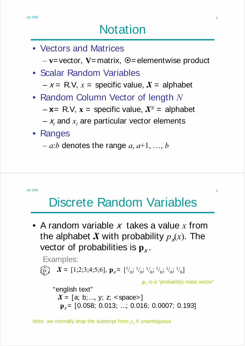
Notation• Vectors and Matrices

– v=vector, V=matrix, =elementwise product

• Scalar Random Variables– x = R.V, x = specific value, X = alphabet

• Random Column Vector of length N– x= R.V, x = specific value, XN = alphabet– xi and xi are particular vector elements

• Ranges– a:b denotes the range a, a+1, …, b

Jan 2008 6

Discrete Random Variables

• A random variable x takes a value x from the alphabet X with probability px(x). The vector of probabilities is px .Examples:

X = [1;2;3;4;5;6], px = [1/6; 1/6; 1/6; 1/6; 1/6; 1/6]

“english text”X = [a; b;…, y; z; <space>]px = [0.058; 0.013; …; 0.016; 0.0007; 0.193]

Note: we normally drop the subscript from px if unambiguous

pX is a “probability mass vector”

Jan 2008 7

Expected Values

• If g(x) is real valued and defined on X then

∑∈

=Xx

xgxpgE )()()(xx

Examples:X = [1;2;3;4;5;6], px = [1/6; 1/6; 1/6; 1/6; 1/6; 1/6]

58.2))((log

3380)1.0sin(

1715

53

2

222

=−=

+==

==

xx

x

x

pE

.E

.E

.E

μσ

μ

This is the “entropy” of X

often write E for EX

Jan 2008 8

Shannon Information Content

• The Shannon Information Content of an outcome with probability p is –log2p

• Example 1: Coin tossing– X = [Heads; Tails], p = [½; ½], SIC = [1; 1] bits

• Example 2: Is it my birthday ?– X = [No; Yes], p = [364/365; 1/365],

SIC = [0.004; 8.512] bitsUnlikely outcomes give more information

Jan 2008 10

Minesweeper

• Where is the bomb ?• 16 possibilities – needs 4 bits to specify

Guess Prob SIC

1. No 15/16 0.093 bits

Jan 2008 11

Entropy

The entropy,– H(x) = the average Shannon Information Content of x– H(x) = the average information gained by knowing its value– the average number of “yes-no” questions needed to find x is in

the range [H(x),H(x)+1)

xxx xx pp 22 log))((log)( TpEH −=−=

H(X ) depends only on the probability vector pX not on the alphabet X, so we can write H(pX)

We use log(x) ≡ log2(x) and measure H(x) in bits– if you use loge it is measured in nats– 1 nat = log2(e) bits = 1.44 bits

•x

e

dx

xdxx 22

2

loglog

)2ln(

)ln()(log ==

Jan 2008 12

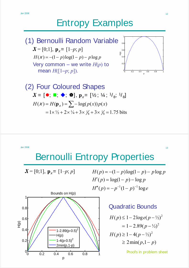
Entropy Examples

(1) Bernoulli Random VariableX = [0;1], px = [1–p; p]

Very common – we write H(p) tomean H([1–p; p]).

(2) Four Coloured ShapesX = [ ; ; ; ], px = [½; ¼; 1/8; 1/8]

ppppH log)1log()1()( −−−−=x

bits75.133¼2½1

)())(log()()(

81

81 =×+×+×+×=

−== ∑ xpxpHH xx p

0 0.2 0.4 0.6 0.8 10

0.2

0.4

0.6

0.8

1

p

H(p

)

Jan 2008 13

Bernoulli Entropy PropertiesX = [0;1], px = [1–p; p]

epppH

pppH

pppppH

log)1()(

log)1log()(

log)1log()1()(

11 −− −−=′′

−−=′−−−−=

Quadratic Bounds

)1,min(2

½)(41)(

½)(89.21

½)(log21)(

2

2

2

pp

ppH

p

pepH

−≥−−≥

−−=

−−≤

Proofs in problem sheet0 0.2 0.4 0.6 0.8 10

0.2

0.4

0.6

0.8

1Bounds on H(p)

p

H(p

)

1-2.89(p-0.5)2

H(p)

1-4(p-0.5)2

2min(p,1-p)

Jan 2008 14

Joint and Conditional Entropy

Joint Entropy: H(x,y)¼0x=1

¼½x=0

y=1y=0p(x,y)

bits 5.1¼log¼0log0¼log¼½log½

),(log),(

=−−−−=−= yxyx pEH

Conditional Entropy : H(y | x)

bits 689.01log¼0log0log¼log½

)|(log)|(

31

32 =−−−−=−= xyxy pEH

Note: 0 log 0 = 0

10x=1

1/32/3x=0

y=1y=0p(y|x)

Note: rows sum to 1

Jan 2008 15

Conditional Entropy – view 1

¼

¾

p(x)

¼0x=1

¼½x=0

y=1y=0p(x, y)Additional Entropy:

{ } { }bits 689.0(¼),¼)0(½,¼,)(),(

)(log),(log

)|(log)|(

)(),()|(

=−=−=−−−=

−=÷=

HHHH

pEpE

pEH

ppp

xyxxyx

xyxyxyxxy

H(Y|X) is the average additional information in Y when you know X

H(y |x)

H(x ,y)

H(x)

Jan 2008 16

Conditional Entropy – view 2

Average Row Entropy:

( ) bits 689.0)0(¼)(¾|)(

)|(log)|()()|(log)|()(

)|(log),()|(log)|(

31

,

,

=×+×===

−=−=

−=−=

∑

∑ ∑∑

∑

∈

∈ ∈

HHxHxp

xypxypxpxypxypxp

xypyxppEH

x

x yyx

yx

X

X Y

xy

xyxy

H(1)

H(1/3)

H(y | x=x)

¼

¾

p(x)

¼0x=1

¼½x=0

y=1y=0p(x, y)

Take a weighted average of the entropy of each row using p(x) as weight

Jan 2008 17

Chain Rules

• Probabilities

• Entropy

The log in the definition of entropy converts products of probability into sums of entropy

)()|(),|(),,( xxyyxzzyx pppp =

∑=

−=

++=n

iiin HH

HHHH

11:1:1 )|()(

)()|(),|(),,(

xxx

xxyyxzzyx

Jan 2008 18

Summary

• Entropy:– Bounded

• Chain Rule:

• Conditional Entropy:

– Conditioning reduces entropy

))((log)())((log)( 22 xpExpxpH Xx

−=−= ∑∈X

x

||log)(0 X≤≤ xH

)()|(),( xxyyx HHH +=

)()|( yxy HH ≤

♦ = inequalities not yet proved

♦

( )∑∈

=−=Xx

xHxpHHH |)()(),()|( yxyxxy

♦

H(x |y) H(y |x)

H(x ,y)

H(x) H(y)

Jan 2008 19

Lecture 2

• Mutual Information– If x and y are correlated, their mutual information is the average

information that y gives about x• E.g. Communication Channel: x transmitted but y received

• Jensen’s Inequality• Relative Entropy

– Is a measure of how different two probability mass vectors are

• Information Inequality and its consequences– Relative Entropy is always positive

• Mututal information is positive• Uniform bound• Conditioning and Correlation reduce entropy

Jan 2008 20

Mutual InformationThe mutual information is the average amount of information that you get about xfrom observing the value of y

);();( xyyx II =

),()()()|()();( yxyxyxxyx HHHHHI −+=−=

Use “;” to avoid ambiguities between I(x;y,z) and I(x,y;z)

Information in x Information in x when you already know y

Mutual information is symmetrical H(x |y) H(y |x)

H(x ,y)

H(x) H(y)

I(x ;y)

Jan 2008 21

Mutual Information Example

• If you try to guess y you have a 50% chance of being correct.

• However, what if you know x ?– Best guess:

H(x |y)=0.5

H(y |x)=0.689

H(x ,y)=1.5

H(x)=0.811 H(y)=1

I(x ;y)=0.311

¼0x=1

¼½x=0

y=1y=0p(x,y)

311.0);(

5.1),(,1)(,811.0)(

),()()(

)|()();(

====

−+=−=

yxyxyx

yxyxyxxyx

I

HHH

HHH

HHI

choose y = x

– If x =0 (p=0.75) then 66% correct prob

– If x =1 (p=0.25) then 100% correct prob

– Overall 75% correct probability

Jan 2008 22

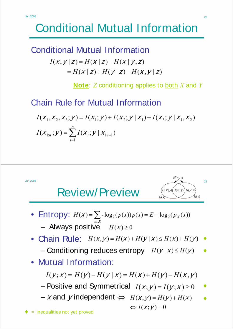
Conditional Mutual Information

Conditional Mutual Information

Note: Z conditioning applies to both X and Y

)|,()|()|(

),|()|()|;(

zyxzyzxzyxzxzyx

HHH

HHI

−+=−=

∑=

−=

++=n

iiin II

IIII

11:1:1

213121321

)|;();(

),|;()|;();();,,(

xyxyx

xxyxxyxyxyxxx

Chain Rule for Mutual Information

Jan 2008 23

Review/Preview

• Entropy:– Always positive

))((log)())((log)( 22 xpExpxp-H Xx

−== ∑∈X

x

0)( ≥xH

)()()|()(),( yxxyxyx HHHHH +≤+=

0);(

)()(),(

=⇔+=

yxxyyx

I

HHH

),()()()|()();( yxyxxyyxy HHHHHI −+=−=

0);();( ≥= xyyx II

)()|( yxy HH ≤

♦ = inequalities not yet proved

♦

♦

♦

♦

H(x |y) H(y |x)

H(x ,y)

H(x) H(y)

I(x ;y)

• Chain Rule:– Conditioning reduces entropy

• Mutual Information:

– Positive and Symmetrical– x and y independent ⇔

Jan 2008 24

Convex & Concave functions

f(x) is strictly convex over (a,b) if

– every chord of f(x) lies above f(x)

– f(x) is concave ⇔ –f(x) is convexConcave is like this

10),,()()1()())1(( <<∈≠∀−+<−+ λλλλλ bavuvfufvuf

),(02

2

baxdx

fd∈∀>

]0[ log,,, 42 ≥xxxexx x

]0[,log ≥xxxx

• Examples– Strictly Convex: – Strictly Concave: – Convex and Concave:

– Test: ⇒ f(x) is strictly convex

“convex” (not strictly) uses “≤” in definition and “≥” in test

Jan 2008 25

Jensen’s Inequality

Jensen’s Inequality: (a) f(x) convex ⇒ Ef(x) ≥ f(Ex)

(b) f(x) strictly convex ⇒ Ef(x) > f(Ex) unless x constant

Proof by induction on |X|

– |X|=1: )()()( 1xfEffE == xx

∑∑−

== −−+==

1

11

)(1

)1()()()(k

ii

k

ikkk

k

iii xf

p

ppxfpxfpfE x

Assume JI is true for |X|=k–1

These sum to 1

Can replace by “>” if f(x) is strictly convex unless pk∈{0,1} or xk = E(x | x∈{x1:k-1})

⎟⎟⎠

⎞⎜⎜⎝

⎛

−−+≥ ∑

−

=

1

1 1)1()(

k

ii

k

ikkk x

p

pfpxfp

( )xEfxp

ppxpf

k

ii

k

ikkk =⎟⎟

⎠

⎞⎜⎜⎝

⎛−

−+≥ ∑−

=

1

1 1)1(

– |X|=k:

Jan 2008 26

Jensen’s Inequality Example

Mnemonic example:f(x) = x2 : strictly convexX = [–1; +1]

p = [½; ½]

E x = 0

f(E x)=0

E f(x) = 1 > f(E x)

-2 -1 0 1 20

1

2

3

4

x

f(x)

Jan 2008 27

Relative Entropy

Relative Entropy or Kullback-Leibler Divergencebetween two probability mass vectors p and q

( ) )()(log)(

)(log

)(

)(log)()||( xx

xx

HqEq

pE

xq

xpxpD

x

−−=== ∑∈

ppqpX

where Ep denotes an expectation performed using probabilities p

D(p||q) measures the “distance” between the probability mass functions p and q. We must have pi=0 whenever qi=0 else D(p||q)=∞Beware: D(p||q) is not a true distance because:

– (1) it is asymmetric between p, q and– (2) it does not satisfy the triangle inequality.

Jan 2008 28

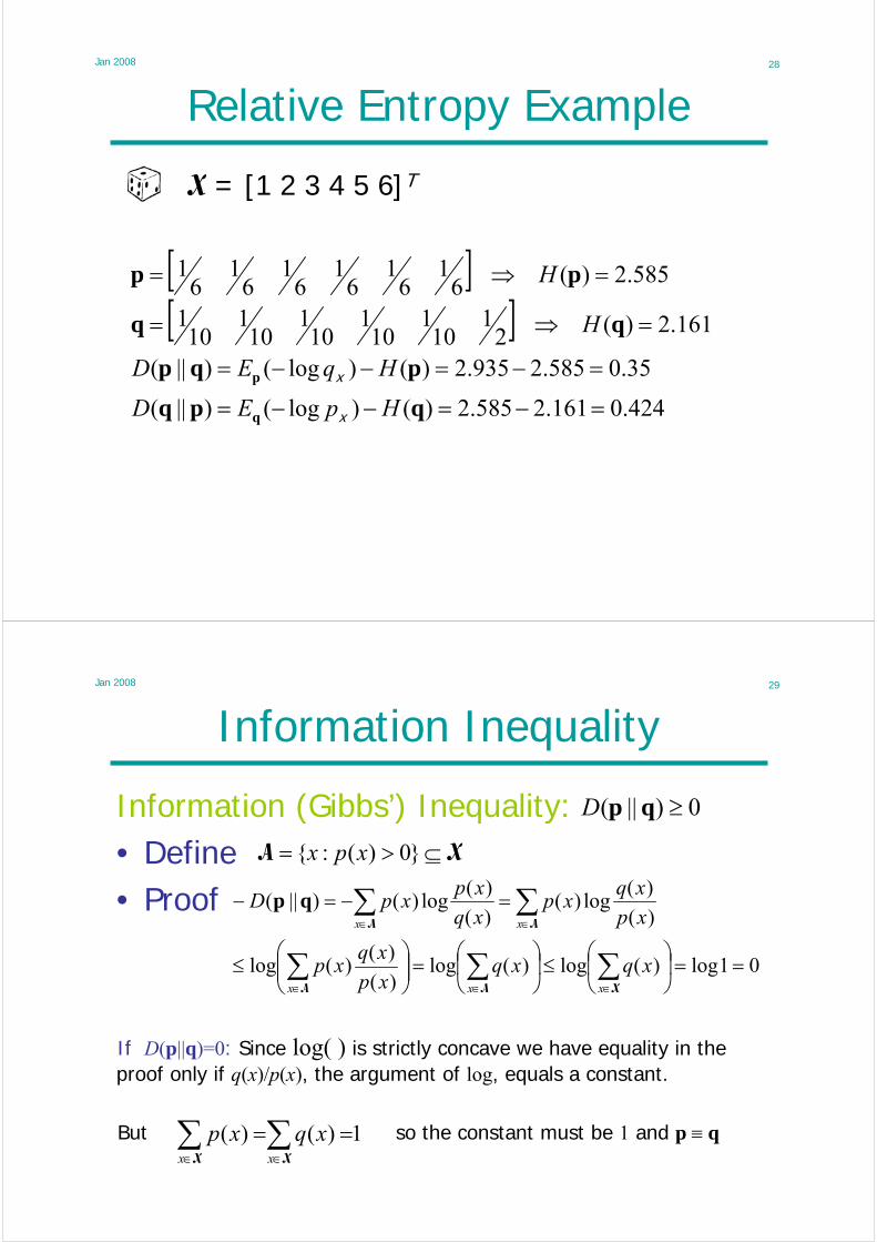
Relative Entropy Example

X = [1 2 3 4 5 6]T

[ ][ ]

424.0161.2585.2)()log()||(

35.0585.2935.2)()log()||(

161.2)(21

101

101

101

101

101

585.2)(61

61

61

61

61

61

=−=−−=

=−=−−=

=⇒=

=⇒=

qpq

pqp

qq

pp

q

p

HpED

HqED

H

H

x

x

Jan 2008 29

Information Inequality

Information (Gibbs’) Inequality:• Define • Proof

0)||( ≥qpD

XA ⊆>= }0)(:{ xpx

01log)(log)(log)(

)()(log

)(

)(log)(

)(

)(log)()||(

==⎟⎠

⎞⎜⎝

⎛≤⎟⎠

⎞⎜⎝

⎛=⎟⎟⎠

⎞⎜⎜⎝

⎛≤

=−=−

∑∑∑

∑∑

∈∈∈

∈∈

XAA

AA

xxx

xx

xqxqxp

xqxp

xp

xqxp

xq

xpxpD qp

If D(p||q)=0: Since log( ) is strictly concave we have equality in the proof only if q(x)/p(x), the argument of log, equals a constant.

But so the constant must be 1 and p ≡ q1)()( ∑∑∈∈

==XX xx

xqxp

Jan 2008 30

Information Inequality Corollaries

• Uniform distribution has highest entropy– Set q = [|X|–1, …, |X|–1]T giving H(q)=log|X| bits

{ } 0)(||log)()(log)||( ≥−=−−= ppqp p HHqED Xx

• Mutual Information is non-negative

0)||(

)()(

),(log),()()();(

, ≥⊗=

=−+=

yxyx

yxyx

yxyxxy

pppD

pp

pEHHHI

with equality only if p(x,y) ≡ p(x)p(y) ⇔ x and y are independent.

Jan 2008 31

More Corollaries

• Conditioning reduces entropy)()|()|()();(0 yxyxyyyx HHHHI ≤⇒−=≤

• Independence Bound

∑∑==

− ≤=n

ii

n

iiin HHH

111:1:1 )()|()( xxxx

with equality only if x and y are independent.

with equality only if all xi are independent.

E.g.: If all xi are identical H(x1:n) = H(x1)

Jan 2008 32

Conditional Independence Bound

• Conditional Independence Bound

• Mutual Information Independence Bound

∑∑==

− ≤=n

iii

n

iniinn HHH

11:11:1:1:1 )|(),|()|( yxyxxyx

If all xi are independent or, by symmetry, if all yi are independent:

∑∑∑===

=−≥

−=n

iii

n

iii

n

ii

nnnnn

IHH

HHI

111

:1:1:1:1:1

);()|()(

)|()();(

yxyxx

yxxyx

E.g.: If n=2 with xi i.i.d. Bernoulli (p=0.5) and y1=x2 and y2=x1, then I(xi;yi)=0 but I(x1:2; y1:2) = 2 bits.

Jan 2008 33

Summary• Mutual Information

0)(

)(log)||( ≥=

xx

q

pED pqp

∑∑==

≤≤n

iiinn

n

iin HHHH

1:1:1

1:1 )|()|()()( yxyxxx

)()|()();( xyxxyx HHHI ≤−=

indep are or if ii

n

iiinn II yxyxyx ∑

=

≥1

:1:1 );();(

• Jensen’s Inequality: f(x) convex ⇒ Ef(x) ≥ f(Ex)

• Relative Entropy:– D(p||q) = 0 iff p ≡ q

• Corollaries– Uniform Bound: Uniform p maximizes H(p)

– I(x ; y) ≥ 0 ⇒ Conditioning reduces entropy

– Indep bounds:

Jan 2008 34

Lecture 3

• Symbol codes– uniquely decodable– prefix

• Kraft Inequality• Minimum code length• Fano Code

Jan 2008 35

Symbol Codes• Symbol Code: C is a mapping X→D+

– D+ = set of all finite length strings from D– e.g. {E, F, G} →{0,1}+ : C(E)=0, C(F)=10, C(G)=11

• Extension: C+ is mapping X+ →D+ formed by concatenating C(xi) without punctuation

• e.g. C+(EFEEGE) =01000110

• Non-singular: x1≠ x2 ⇒ C(x1) ≠ C(x2)

• Uniquely Decodable: C+ is non-singular– that is C+(x+) is unambiguous

Jan 2008 36

Prefix Codes

• Instantaneous or Prefix Code:No codeword is a prefix of another

• Prefix ⇒ Uniquely Decodable ⇒ Non-singular

Examples:UP

PU

UP

PU

UP

– C(E,F,G,H) = (0, 1, 00, 11)

– C(E,F) = (0, 101)

– C(E,F) = (1, 101)

– C(E,F,G,H) = (00, 01, 10, 11)

– C(E,F,G,H) = (0, 01, 011, 111)

Jan 2008 37

Code Tree

Prefix code: C(E,F,G,H) = (00, 11, 100, 101)

1

0

0

0

1

1

E

F

G

H

0

1

– D branches at each node– Each node along the path to

a leaf is a prefix of the leaf⇒ can’t be a leaf itself

– Some leaves may be unusedall used ⇒

111011000000→ FHGEE

Form a D-ary tree where D = |D|

1 of multiple a is 1|| −− DX

Jan 2008 38

Kraft Inequality (binary prefix)

• Label each node at depth l with 2–l

1

0

0

0

1

1

E

F

G

H

0

1

½

½

¼

¼

¼

¼

1/8

1/8

1

• Each node equals the sum of all its leaves

• Codeword lengths:l1, l2, …, l|X| ⇒ 12

||

1

≤∑=

−X

i

li

• Equality iff all leaves are utilised• Total code budget = 1

Code 00 uses up ¼ of the budgetCode 100 uses up 1/8 of the budget

Same argument works with D-ary tree

Jan 2008 40

Kraft Inequality

If uniquely decodable C has codeword lengths

l1, l2, …, l|X| , then

Proof: Let

1||

1

≤∑=

−X

i

liD

,NlMDS ii

li any for then and max||

1

==∑=

−X

( )∑∑ ∑∑= = =

+++−

=

− =⎟⎟⎠

⎞⎜⎜⎝

⎛=

||

1

||

1

||

1

||

1 1 2

21

X X XX

i i i

lll

N

i

lN

N

Niiii DDS

If S > 1 then SN > NM for some N. Hence S ≤ 1

∑∈

− +

=N

CDXx

x)}(length{

∑=

+− ==NM

l

l ClD1

|)}(length{:| xx ∑=

−≤NM

l

ll DD1

NMNM

l

==∑=1

1

Jan 2008 41

Converse to Kraft Inequality

If then ∃ a prefix code withcodeword lengths l1, l2, …, l|X|

Proof:– Assume li ≤ li+1 and think of codewords as

base-D decimals 0.d1d2…dli

– Let codeword with lk digits

–

– So cj cannot be a prefix of ck because they differ in the first lj digits.

1||

1

≤∑=

−X

i

liD

∑−

=

−=1

1

k

i

lk

iDc

⇒ non-prefix symbol codes are a waste of time

jil

j

k

ji

ljk DcDcckj −

−

=

− +≥+=< ∑1

have we any For

Jan 2008 42

Kraft Converse Example

Suppose l = [2; 2; 3; 3; 3] ⇒ 1875.02|5

1

≤=∑=

−

i

li

1100.75 = 0.11023

1010.625 = 0.10123

1000.5 = 0.10023

010.25 = 0.0122

000.0 = 0.0022

Codelk ∑−

=

−=1

1

k

i

lk

iDc

Each ck is obtained by adding 1 to the LSB of the previous row

For code, express ck in binary and take the first lk binary places

Jan 2008 44

Minimum Code Length

If l(x) = length(C(x)) then C is optimal ifLC=E l(X) is as small as possible.

Uniquely decodable code ⇒ LC ≥ H(X)/log2D

Proof:)(log)(log/)( 2 xxx pElEDHL DC +=−

We define q by

with equality only if c=1 and D(p||q) = 0 ⇒ p = q ⇒ l(x) = –logD(x)

1 where)( )()(1 ≤== ∑ −−−

x

xlxl DcDcxq

( ) ( ))(log)(log)(loglog )( xxxx pcqEpDE DDDl

D +−=+−= −

cq

pE DD log

)(

)(log −⎟⎟

⎠

⎞⎜⎜⎝

⎛=

xx ( )( ) 0log||2log ≥−= cDD qp

Jan 2008 45

Fano Code

Fano Code (also called Shannon-Fano code)1. Put probabilities in decreasing order2. Split as close to 50-50 as possible; repeat with each half

0.20

0.19

0.17

0.15

0.14

a

b

c

d

e

0

10.06

0.05

0.04

f

g

h

0

10

1

0

1

0

1

0

10

1

00

010

011

100

101

110

1110

1111

H(p) = 2.81 bits

LSF = 2.89 bits

Always

Not necessarily optimal: the best code for this p actually has L = 2.85 bits

1)(

)min(21)()(

+≤−+≤≤

p

ppp

H

HLH F

Jan 2008 46

Summary

• Kraft Inequality for D-ary codes:– any uniquely decodable C has

– If then you can create a prefix code

1||

1

≤∑=

−X

i

liD

1||

1

≤∑=

−X

i

liD

• Uniquely decodable ⇒ LC ≥ H(X)/log2D

• Fano code– Order the probabilities, then repeatedly split in half to

form a tree.

– Intuitively natural but not optimal

Jan 2008 47

Lecture 4

• Optimal Symbol Code– Optimality implications– Huffman Code

• Optimal Symbol Code lengths– Entropy Bound

• Shannon Code

Jan 2008 48

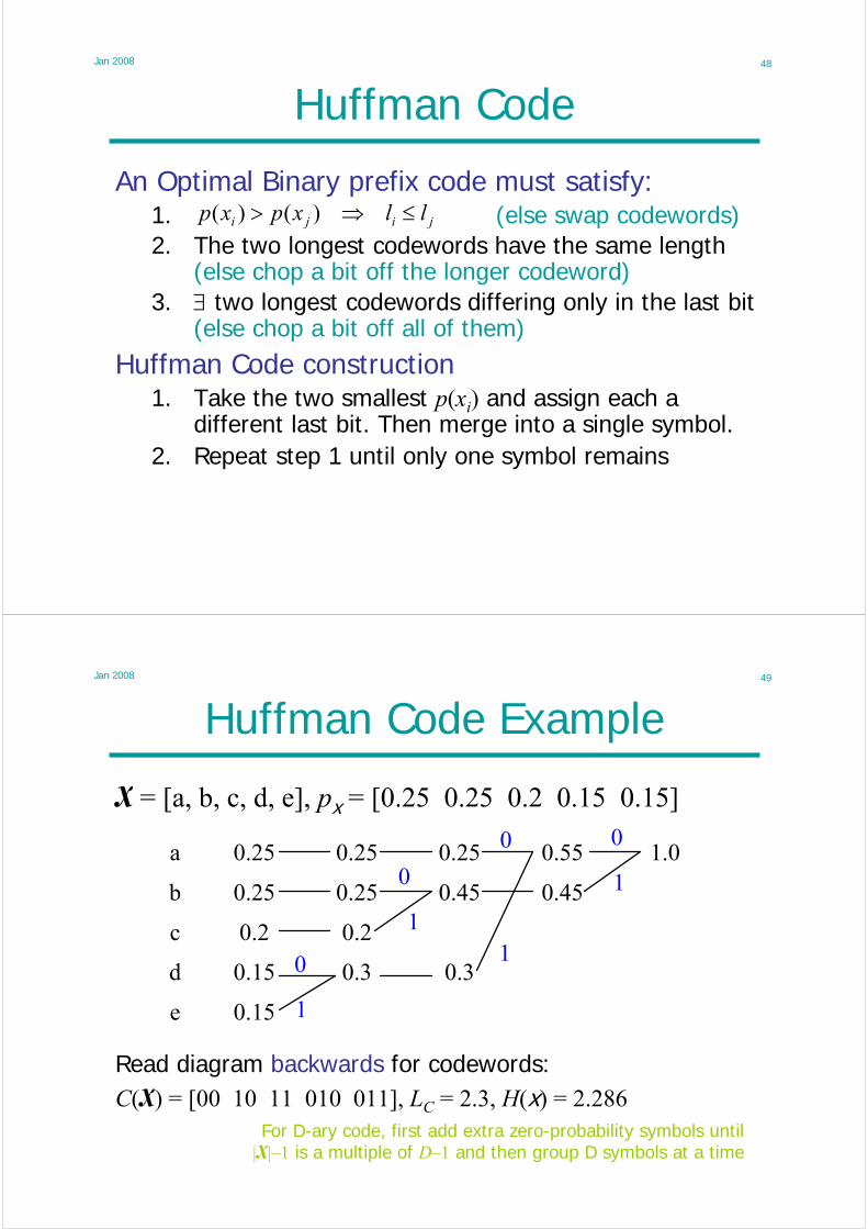
Huffman Code

An Optimal Binary prefix code must satisfy:1. (else swap codewords)jiji llxpxp ≤⇒> )()(

2. The two longest codewords have the same length(else chop a bit off the longer codeword)

3. ∃ two longest codewords differing only in the last bit(else chop a bit off all of them)

Huffman Code construction1. Take the two smallest p(xi) and assign each a

different last bit. Then merge into a single symbol.2. Repeat step 1 until only one symbol remains

Jan 2008 49

Huffman Code Example

X = [a, b, c, d, e], px = [0.25 0.25 0.2 0.15 0.15]

0.25

0.25

0.2

0.15

0.15

0.25

0.25

0.2

0.3

0.25

0.45

0.3

0.55

0.45

1.0a

b

c

d

e

0

1

0

0 0

11

1

Read diagram backwards for codewords:C(X) = [00 10 11 010 011], LC = 2.3, H(x) = 2.286

For D-ary code, first add extra zero-probability symbols until |X|–1 is a multiple of D–1 and then group D symbols at a time

Jan 2008 51

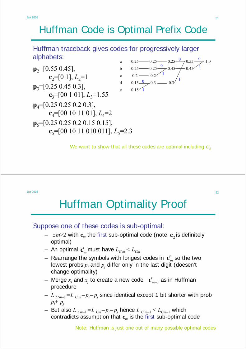
Huffman Code is Optimal Prefix Code

p2=[0.55 0.45],c2=[0 1], L2=1

Huffman traceback gives codes for progressively larger alphabets:

We want to show that all these codes are optimal including C5

p3=[0.25 0.45 0.3],c3=[00 1 01], L3=1.55

p4=[0.25 0.25 0.2 0.3],c4=[00 10 11 01], L4=2

p5=[0.25 0.25 0.2 0.15 0.15],c5=[00 10 11 010 011], L5=2.3

0.25

0.25

0.2

0.15

0.15

0.25

0.25

0.2

0.3

0.25

0.45

0.3

0.55

0.45

1.0a

b

c

d

e

0

1

0

0 0

11

1

Jan 2008 52

Suppose one of these codes is sub-optimal:– ∃m>2 with cm the first sub-optimal code (note is definitely

optimal)

Huffman Optimality Proof

Note: Huffman is just one out of many possible optimal codes

2c

mc′mc′

1−′mc

– An optimal must have LC'm < LCm

– Rearrange the symbols with longest codes in so the two lowest probs pi and pj differ only in the last digit (doesen’tchange optimality)

– Merge xi and xj to create a new code as in Huffman procedure

– L C'm–1 =L C'm– pi– pj since identical except 1 bit shorter with probpi+ pj

– But also L Cm–1 =L Cm– pi– pj hence L C'm–1 < LCm–1 which contradicts assumption that cm is the first sub-optimal code

Jan 2008 53

How short are Optimal Codes?

Huffman is optimal but hard to estimate its length.If l(x) = length(C(x)) then C is optimal if

LC=E l(x) is as small as possible.

We want to minimize subject to

1.

2. all the l(x) are integers

Simplified version:Ignore condition 2 and assume condition 1 is satisfied with equality.

∑∈Xx

xlxp )()(

1)( ≤∑∈

−

Xx

xlD

less restrictive so lengths may be shorter than actually possible ⇒ lower bound

Jan 2008 54

Optimal Codes (non-integer li)

• Minimize subject to∑=

||

1

)(X

iii lxp

0 )(||

1

||

1

=∂∂

+= ∑∑=

−

= ii

l

iii l

JDlxpJ i set and Define

XX

λ

)ln(/)(0)ln()( DxpDDDxpl

Ji

lli

i

ii λλ =⇒=−=∂∂ −−

1||

1

=∑=

−X

i

liD

( ) ( )D

H

D

pEpElEl Di

22

2

log

)(

log

)(log)(log)(,

xxxx =−

=−= these with

no uniquely decodable code can do better than this (Kraft inequality)

li = –logD(p(xi))⇒=⇒=∑=

− )ln(/11||

1

DDi

li λX

also

Use lagrange multiplier:

Jan 2008 55

Shannon Code

Round up optimal code lengths:• li are bound to satisfy the Kraft Inequality (since the

optimum lengths do)

⎡ ⎤)(log iDi xpl −=

or ∑∑−

=

−

=

− ==1

1

1

1

)(k

iik

k

i

lk xpcDc i

1log

)(

log

)(

22

+<≤D

XHL

D

XHC

(since we added <1to optimum values)

Note: since Huffman code is optimal, it also satisfies these limits

• Hence prefix code exists:put li into ascending order and set

to li places

• Average length:

equally good

since ili Dxp −≥)(

Jan 2008 56

Shannon Code Examples

Example 1(good)

⎡ ⎤bits 08.0)( bits, 06.1

]71[log

]64.60145.0[log

]01.099.0[

2

2

===−==−=

xxx

x

x

HLC

pl

p

pExample 2(bad)

⎡ ⎤bits 75.1)( bits, 75.1

]3321[log

]3321[log

]125.0125.025.05.0[

2

2

===−==−=

xxx

x

x

HLC

pl

p

p

We can make H(x)+1 bound tighter by encoding longer blocks as a super-symbol

Dyadic probabilities

(obviously stupid to use 7)

Jan 2008 57

Shannon versus Huffman

Shannon

0.36

0.34

0.25

0.05

0.36

0.34

0.3

0.36

0.64

1.0a

b

c

d

0

0

0

1

1

1

⎡ ⎤bits 15.2

]5222[log

]32.4256.147.1[log

bits 78.1)(]05.025.034.036.0[

2

2

==−==−

=⇒=

S

S

L

H

x

x

x x

pl

p

p

Huffman

bits 94.1

]3321[

==

H

H

L

l

Individual codewords may be longer in Huffman than Shannon but not the average

Jan 2008 58

Shannon Competitive Optimality

• l(x) is length of a uniquely decodable code• is length of Shannon code

then⎡ ⎤)(log)( xpxlS −=

( ) cS cllp −≤−≤ 12)()( xx

⎡ ⎤( ) ( ) )(1)(log)()(log)( A∈=+−−<≤−−≤ xpcplpcplp xxxx

No other symbol code can do much better than Shannon code most of the time

Kraft inequality

}2)(:{ Define 1)( +−−<= cxlxpxA x with especially short l(x)Proof:

)1()()1(1)( 2222 −−−−−+−− ≤=≤ ∑∑ c

x

xlc

x

cxl

∑∑∑∈

+−−

∈∈

<∈≤=AAA

Ax

cxl

xx

xxpxp 1)(2)|)(max()(

now over all x

Jan 2008 59

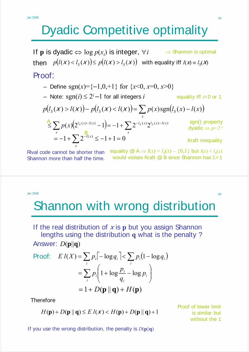
Dyadic Competitive optimality

If p is dyadic ⇔ log p(xi) is integer, ∀i

then ( ) ( ))()()()( xxxx SS llpllp >≤<

01121 )( =+−≤+−= ∑ −

x

xl

with equality iff l(x) ≡ lS(x)

Kraft inequality

equality iff i=0 or 1

sgn() propertydyadic ⇒ p=2–l

Rival code cannot be shorter than Shannon more than half the time.

⇒ Shannon is optimal

Proof:– Define sgn(x)={–1,0,+1} for {x<0, x=0, x>0}

– Note: sgn(i) ≤ 2i –1 for all integers i

( ) ( ) ( )∑ −=<−>x

SSS xlxlxpllpllp )()(sgn)()()()()( xxxx

( ) ∑∑ −−− +−=−≤x

xlxlxl

x

xlxl SSSxp )()()()()( 22112)(

equality @ A ⇒ l(x) = lS(x) – {0,1} but l(x) < lS(x)would violate Kraft @ B since Shannon has Σ=1

A

B

Jan 2008 60

Shannon with wrong distribution

If the real distribution of x is p but you assign Shannon lengths using the distribution q what is the penalty ?

Answer: D(p||q)

⎡ ⎤ ( )∑∑ −<−=i

iii

ii qpqpXlE log1log)(

Therefore

1)||()()()||()( ++<≤+ qppqpp DHlEDH xProof of lower limit

is similar butwithout the 1

If you use the wrong distribution, the penalty is D(p||q)

Proof:

∑ ⎟⎟⎠

⎞⎜⎜⎝

⎛−+=

ii

i

ii p

q

pp loglog1

)()||(1 pqp HD ++=

Jan 2008 61

Summary

• Any uniquely decodable code:D

HHlE D

2log

)()()(

xxx =≥

⎡ ⎤iDi pl log−= 1)()()( +≤≤ xxx DD HlEH

1)()()( +≤≤ xxx DD HlEH• Fano Code:

– Intuitively natural top-down design

• Huffman Code:

– Bottom-up design

– Optimal ⇒ at least as good as Shannon/Fano

• Shannon Code:

– Close to optimal and easier to prove bounds

Note: Not everyone agrees on the names of Shannon and Fano codes

Jan 2008 62

Lecture 5

• Stochastic Processes• Entropy Rate• Markov Processes• Hidden Markov Processes

Jan 2008 63

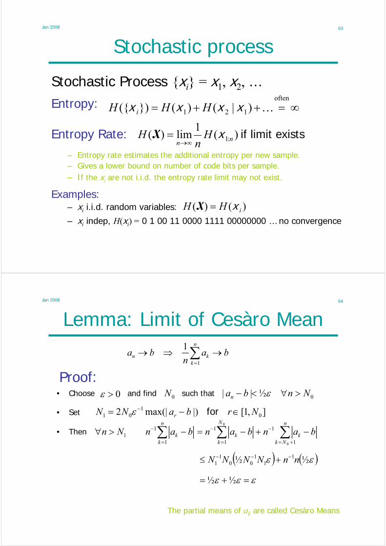
Stochastic process

Stochastic Process {xi} = x1, x2, …Entropy:

Entropy Rate:

– Entropy rate estimates the additional entropy per new sample.– Gives a lower bound on number of code bits per sample.– If the xi are not i.i.d. the entropy rate limit may not exist.

Examples:– xi i.i.d. random variables:

– xi indep, H(xi) = 0 1 00 11 0000 1111 00000000 … no convergence

∞=++=often

121 )|()(})({ …xxxx HHH i

existslimit if )(1

lim)( :1 nn

Hn

H x∞→

=X

)()( iHH x=X

Jan 2008 64

Lemma: Limit of Cesàro Mean

Proof:

ban

ban

kkn →⇒→ ∑

=1

1

• Choose and find such that 0>ε 0N 0½|| Nnban >∀<− ε

],1[|)max(|2 01

01 NrbaNN r ∈−= − for ε

∑∑∑+=

−

=

−

=

− −+−=−>∀n

Nkk

N

kk

n

kk banbanbanNn

1

1

1

1

1

11

0

0

The partial means of ak are called Cesàro Means

• Set

• Then

( ) ( )εε ½½ 11

100

11 nnNNNN −−− +≤

εεε =+= ½½

Jan 2008 65

Stationary Process

Stochastic Process {xi} is stationary iff

X∈∀=== + innknn ankapap ,,)()( :1):1(:1:1 xx

If {xi} is stationary then H(X) exists and

)|(lim)(1

lim)( 1:1:1 −∞→∞→== nn

nn

nHH

nH xxxX

Proof: )|()|()|(0 2:11

)b(

1:2

)a(

1:1 −−−− =≤≤ nnnnnn HHH xxxxxx

Hence H(xn|x1:n-1) is +ve, decreasing ⇒ tends to a limit, say b

(a) conditioning reduces entropy, (b) stationarity

)()|(1

)(1

)|(1

1:1:11:1 XHbHn

Hn

bHn

kkknkk =→=⇒→ ∑

=−− xxxxx

Hence from Cesàro Mean lemma:

Jan 2008 66

Block Coding

If xi is a stochastic process– encode blocks of n symbols– 1-bit penalty of Shannon/Huffman is now shared

between n symbols 1

:11

:11

:11 )()()( −−−− +≤≤ nHnlEnHn nnn xxx

If entropy rate of xi exists (⇐ xi is stationary)

)()()()( :11

:11 XX HlEnHHn nn →⇒→ −− xx

The extra 1 bit inefficiency becomes insignificant for large blocks

Jan 2008 67

Block Coding Example

• n=1codeprobsym

100.10.9BA

11 =− lEn

• n=2

110.09AB

1000.09BA

codeprobsym

10100.010.81BBAA

645.01 =− lEn

• n=3

………

1010.081AAB

100100.009BBA

codeprobsym

1001100.0010.729BBBAAA

583.01 =− lEn

2 4 6 8 10 120.4

0.6

0.8

1

n-1E

l

n

469.0)( =ixH

X = [A;B], px = [0.9; 0.1]

Jan 2008 68

Markov Process

Discrete-valued Stochastic Process {xi} is• Independent iff p(xn|x0:n–1)=p(xn)

• Markov iff p(xn|x0:n–1)=p(xn|xn–1)

1

3 4

2t12

t13t24

t14

t34

t43

Independent Stochastic Process is easiest to deal with, Markov is next easiest

– time-invariant iff p(xn=b|xn–1=a) = pab indep of n

– Transition matrix: T = {tab}• Rows sum to 1: T1 = 1 where 1 is a vector of 1’s• pn = TTpn–1

• Stationary distribution: p$ = TTp$

Jan 2008 69

Stationary Markov Process

If a Markov process isa) irreducible: you can go from any a to any b

in a finite number of steps• irreducible iff (I+TT)|X|–1 has no zero entries

b) aperiodic: ∀a, the possible times to go from a to a have highest common factor = 1

$$ ppT =T

TT

n

n ]111[$ =→∞→

11pT where

then it has exactly one stationary distribution, p$.– p$ is the eigenvector of TT with λ = 1:–

Jan 2008 71

H(p1)=0, H(p

1 | p

0)=0

Chess Board

Random Walk• Move equal prob• p1 = [1 0 … 0]T

– H(p1) = 0

• p$ = 1/40 × [3 5 3 5 8 5 3 5 3]T

– H(p$) = 3.0855

•

–

)log()|(lim)( ,,

,$,1 jiji

jiinnn

ttpHH ∑−== −∞→xxX

2365.2)( =XH

Time-invariant and p1 = p$ ⇒ stationary

Jan 2008 72

Chess Board FramesH(p

1)=0, H(p

1 | p

0)=0 H(p

2)=1.58496, H(p

2 | p

1)=1.58496 H(p

3)=3.10287, H(p

3 | p

2)=2.54795 H(p

4)=2.99553, H(p

4 | p

3)=2.09299

H(p5)=3.111, H(p

5 | p

4)=2.30177 H(p

6)=3.07129, H(p

6 | p

5)=2.20683 H(p

7)=3.09141, H(p

7 | p

6)=2.24987 H(p

8)=3.0827, H(p

8 | p

7)=2.23038

Jan 2008 73

ALOHA Wireless Example

M users share wireless transmission channel– For each user independently in each timeslot:

• if its queue is non-empty it transmits with prob q• a new packet arrives for transmission with prob p

– If two packets collide, they stay in the queues– At time t, queue sizes are xt = (n1, …, nM)

• {xt} is Markov since p(xt) depends only on xt–1

Transmit vector is yt :

– {yt} is not Markov since p(yt) is determined by xt but is not determined by yt–1. {yt} is called a Hidden Markov Process.

⎩⎨⎧

>=

==0

00)1(

,

,,

ti

titi xq

xyp

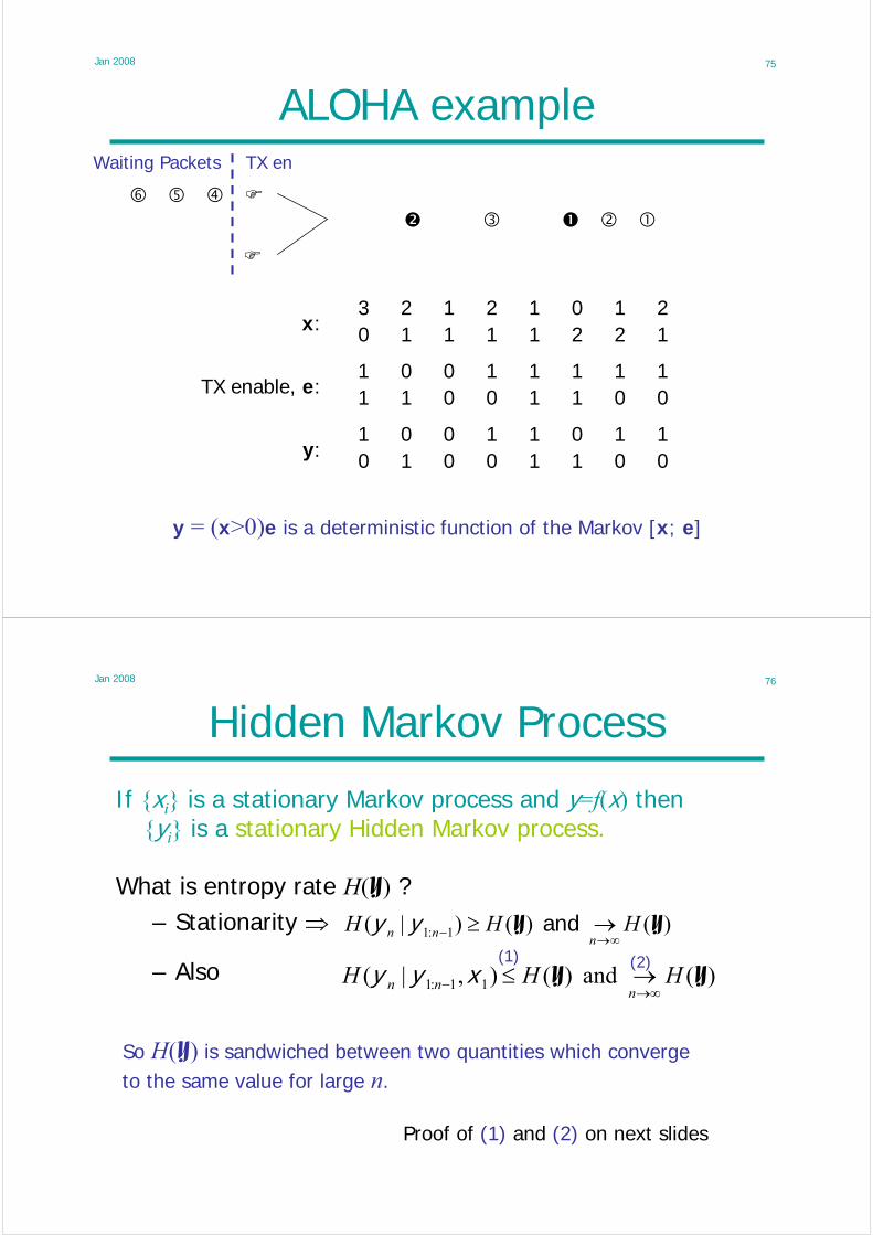
Jan 2008 75

ALOHA example

x:

TX enable, e:

y:

y = (x>0)e is a deterministic function of the Markov [x; e]

Waiting Packets TX en

3 2 1 2 1 0 1 20 1 1 1 1 2 2 1

1 0 0 1 1 1 1 11 1 0 0 1 1 0 0

1 0 0 1 1 0 1 10 1 0 0 1 1 0 0

Jan 2008 76

Hidden Markov Process

If {xi} is a stationary Markov process and y=f(x) then{yi} is a stationary Hidden Markov process.

What is entropy rate H(Y) ?)( )()|( 1:1 YY HHH

nnn ∞→− →≥ andyy

)( and )(),|( 11:1 YY HHHn

nn ∞→− →≤xyy(1) (2)

So H(Y) is sandwiched between two quantities which converge to the same value for large n.

Proof of (1) and (2) on next slides

– Stationarity ⇒

– Also

Jan 2008 77

Hidden Markov Process – (1)

Proof (1): )(),|( 11:1 YHH nn ≤− xyy

)()|( 1:0 YHHk

nknk ∞→−++ →= yy

x markov

y=f(x)

conditioning reduces entropy

y stationary

kHH knnnn ∀= −−− ),|(),|( 1:1:111:1 xyyxyy

),|(),,|( 1:1:1:1:1:1 knknkknn HH −−−−−− == xyyyxyy

kH nkn ∀≤ −− )|( 1:yy

Just knowing x1 in addition to y1:n–1 reduces the conditional entropy to below the entropy rate.

Jan 2008 78

Hidden Markov Process – (2)

Proof (2): )(),|( 11:1 YHHn

nn ∞→− →xyy

defn of I(A;B)

The influence of x1 on yn decreases over time.

0)(

)|;()|(),|( 1:111:111:1

−→−=

∞→

−−−

YH

IHH

n

nnnnnn yyxyyxyy

);()|;( :111

1:11 k

k

nnn II yxyyx =∑

=−Note that

0)|;( 1:11 ∞→− →n

nnI yyxHence

)( 1xH≤

chain rule

bounded sum ofnon-negative terms

So defn of I(A;B)

Jan 2008 79

Summary

• Entropy Rate: )(1

lim)( :1 nn

Hn

H x∞→

=X

)|(lim)( 1:1 −∞→= nn

nHH xxX

)log()|()( ,,

,$,1 jiji

jiinn ttpHH ∑−== −xxX

)|( )(),|( 1:111:1 −− ≤≤ nnnn HHH yyxyy Y

with both sides tending to H(Y)

if it exists

– {xi} stationary:

– {xi} stationary Markov:

– y = f(x): Hidden Markov:

Jan 2008 80

Lecture 6

• Stream Codes• Arithmetic Coding• Lempel-Ziv Coding

Jan 2008 81

Huffman: Good and Bad

Good– Shortest possible symbol code 1

log

)(

log

)(

22

+≤≤D

HL

D

HS

xx

Bad– Redundancy of up to 1 bit per symbol

• Expensive if H(x) is small• Less so if you use a block of N symbols• Redundancy equals zero iff p(xi)=2–k(i) ∀i

– Must recompute entire code if any symbol probability changes• A block of N symbols needs |X|N pre-calculated

probabilities

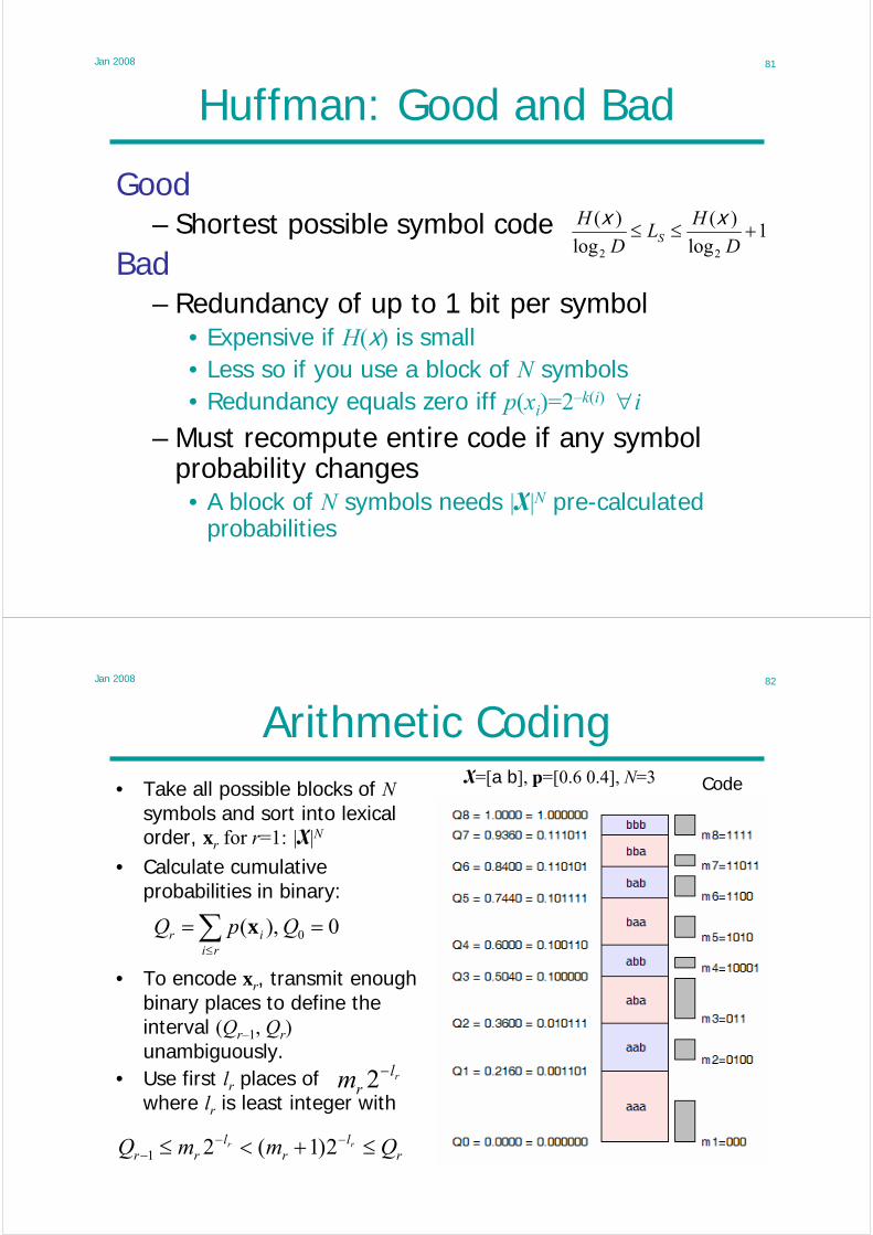
Jan 2008 82

• To encode xr, transmit enough binary places to define the interval (Qr–1, Qr)unambiguously.

Arithmetic Coding• Take all possible blocks of N

symbols and sort into lexical order, xr for r=1: |X|N

• Calculate cumulative probabilities in binary:

X=[a b], p=[0.6 0.4], N=3 Code

0,)( 0 ==∑≤

QpQri

ir x

rlrm −2

rl

rl

rr QmmQ rr ≤+<≤ −−− 2)1(21

• Use first lr places ofwhere lr is least integer with

Jan 2008 83

bab

bba

bbb

Q5 = 0.7440 = 0.101111

Q6 = 0.8400 = 0.110101

Q7 = 0.9360 = 0.111011

m6=1100

m7=11011

m8=1111

• The interval corresponding to xr has width

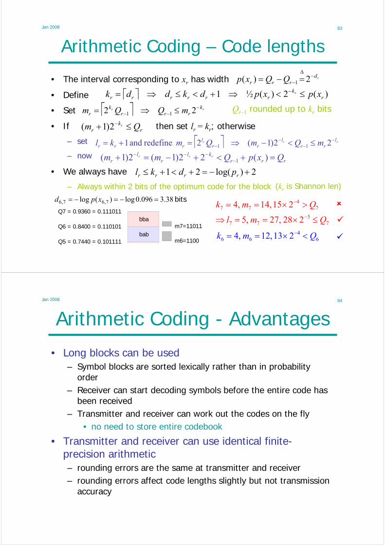
Arithmetic Coding – Code lengthsrd

rrr QQxp −Δ

− =−= 2)( 1

⎡ ⎤ )(2)(½1 rk

rrrrrr xpxpdkddk r ≤<⇒+<≤⇒= −

⎡ ⎤ rr krrr

kr mQQm −

−− ≤⇒= 22 11

rk

r Qm r ≤+ −2)1(

⎡ ⎤ rrr lrr

lrr

lrrr mQmQmkl −

−−

− ≤<−⇒=+= 22)1(2 redefine and 1 11

rrrkl

rl

r QxpQmm rrr =+<+−=+ −−−− )(22)1(2)1( 1

2)log(21 +−=+<+≤ rrrr pdkl

64

66 213,12,4 Qmk <×== −

75

77

74

77

228,27,5

215,14,4

Qml

Qmk

≤×==⇒

>×==−

−bits 38.3096.0log)(log 7,67,6 =−=−= xpd

• Define

• Set

• If then set lr = kr; otherwise

– set

– now

• We always have

– Always within 2 bits of the optimum code for the block

Qr–1 rounded up to kr bits

(kr is Shannon len)

Jan 2008 84

Arithmetic Coding - Advantages

• Long blocks can be used– Symbol blocks are sorted lexically rather than in probability

order– Receiver can start decoding symbols before the entire code has

been received– Transmitter and receiver can work out the codes on the fly

• no need to store entire codebook

• Transmitter and receiver can use identical finite-precision arithmetic – rounding errors are the same at transmitter and receiver– rounding errors affect code lengths slightly but not transmission

accuracy

Jan 2008 85

a

b

aa

ab

ba

bb

aaa

aab

aba

abb

baa

bab

bba

bbb

aaaa

aaab

aaba

aabb

abaa

abab

abbaabbb

baaa

baab

babababbbbaabbabbbba

0.0000 = 0.000000

0.1296 = 0.001000

0.2160 = 0.001101

0.3024 = 0.010011

0.3600 = 0.010111

0.4464 = 0.011100

0.5040 = 0.100000

0.5616 = 0.1000110.6000 = 0.100110

0.6864 = 0.101011

0.7440 = 0.101111

0.8016 = 0.1100110.8400 = 0.110101

0.8976 = 0.1110010.9360 = 0.1110110.9744 = 0.111110

Arithmetic Coding Receiver

X=[a b], p=[0.6 0.4]

Qr probabilities

1 1 0 0 1 1 1

b

babbabbaa

Each additional bit received narrows down the possible interval.

Jan 2008 86

Transmitter Send ReceiverInput Min Max Min Test Max Output

00000000 11111111 00000000 10011001 11111111b 10011001 11111111 1 10011001a 10011001 11010111b 10111110 11010111b 11001101 11010111 10 10011001 ba 11001101 11010011 10011001 11010111 11111111a 11001101 11010000a 11001101 11001111 011 11010111 a

10011001 10111110 11010111 bb 11001110 11001111 1 10111110 11001101 11010111 b

11001101 11010011 11010111 a11001101 11010000 11010011 a11001101 11001111 11010000

… … … … … … …

Arithmetic Coding/Decoding

• Min/Max give the limits of the input or output interval; identical in transmitter and receiver.• Blue denotes transmitted bits - they are compared with the corresponding bits of the receiver’s test

value and Red bit show the first difference. Gray identifies unchanged words.

Jan 2008 87

Arithmetic Coding AlgorithmInput Symbols: X = [a b], p = [p q]

[min , max] = Input Probability RangeNote: only keep untransmitted bits of min and max

Coding Algorithm:Initialize [min , max] = [000…0 , 111…1]

For each input symbol, sIf s=a then max=min+p(max–min) else min=min+p(max–min)

while min and max have the same MSBtransmit MSB and set min=(min<<1) and max=(max<<1)+1

end whileend for

• Decoder is almost identical. Identical rounding errors ⇒ no symbol errors.• Simple to modify algorithm for |X|>2 and/or D>2.• Need to protect against range underflow when [x y] = [011111…, 100000…].

Jan 2008 88

Adaptive Probabilities

Number of guesses for next letter (a-z, space):o r a n g e s a n d l e mo n s

17 7 8 4 1 1 2 1 1 5 1 1 1 1 1 1 1 1

We can change the input symbol probabilities based on the context (= the past input sequence)

n

xp

ini

n +

=+= <≤

1

)(count11

b

Example: Bernoulli source with unknown p. Adapt p based on symbol frequencies so far:

X = [a b], pn = [1–pn pn],

Jan 2008 89

Adaptive Arithmetic Coding

Coder and decoder only need to calculate the probabilities along the path that actually occurs

a

b

aa

ab

ba

bb

aaa

aab

aba

abb

baa

bab

bba

bbb

aaaa

aaab

aabaaabbabaaabababbaabbb

baaabaabbabababbbbaabbab

bbba

bbbb

0.0000 = 0.000000

0.2000 = 0.001100

0.2500 = 0.010000

0.3000 = 0.0100110.3333 = 0.010101

0.3833 = 0.0110000.4167 = 0.0110100.4500 = 0.011100

0.5000 = 0.011111

0.5500 = 0.1000110.5833 = 0.1001010.6167 = 0.100111

0.6667 = 0.1010100.7000 = 0.101100

0.7500 = 0.110000

0.8000 = 0.110011

1.0000 = 0.000000

p1 = 0.5

p2 = 1/3 or 2/3

p3 = ¼ or ½ or ¾

p4 = …

n

xp

ini

n +

=+= <≤

1

)(count11

b

Jan 2008 90

Lempel-Ziv Coding

Memorize previously occurring substrings in the input data– parse input into the shortest possible distinct ‘phrases’– number the phrases starting from 1 (0 is the empty string)

1011010100010…12_3_4__5_6_7

– each phrase consists of a previously occurring phrase(head) followed by an additional 0 or 1 (tail)

– transmit code for head followed by the additional bit for tail01001121402010…

– for head use enough bits for the max phrase number so far:100011101100001000010…

– decoder constructs an identical dictionary

prefix codes are underlined

Jan 2008 91

Input = 1011010100010010001001010010

Dictionary Send Decode

0000 φ 1 10001 1 00 00010 0 011 110011 11 101 010100 01 1000 0100101 010 0100 000110 00 0010 100111 10 1010 01001000 0100 10001 010011001 01001

Input = 1011010100010010001001010010


00 φ 1 101 1 00 010 0

Input = 1011010100010010001001010010


00 φ 1 101 1 00 010 0 011 11

Input = 1011010100010010001001010010


00 φ 1 101 1 00 010 0 011 1111 11

Input = 1011010100010010001001010010


00 φ 1 101 1 00 010 0 011 1111 11 101 01

Lempel-Ziv Example

Input = 1011010100010010001001010010


φ 1 1

Input = 1011010100010010001001010010


0 φ 1 11 1 00 0

Input = 1011010100010010001001010010


000 φ 1 1001 1 00 0010 0 011 11011 11 101 01100 01

Input = 1011010100010010001001010010


000 φ 1 1001 1 00 0010 0 011 11011 11 101 01100 01

Input = 1011010100010010001001010010


000 φ 1 1001 1 00 0010 0 011 11011 11 101 01100 01 1000 010

Input = 1011010100010010001001010010


000 φ 1 1001 1 00 0010 0 011 11011 11 101 01100 01 1000 010101 010

Input = 1011010100010010001001010010


000 φ 1 1001 1 00 0010 0 011 11011 11 101 01100 01 1000 010101 010 0100 00

Input = 1011010100010010001001010010


000 φ 1 1001 1 00 0010 0 011 11011 11 101 01100 01 1000 010101 010 0100 00110 00

Input = 1011010100010010001001010010


000 φ 1 1001 1 00 0010 0 011 11011 11 101 01100 01 1000 010101 010 0100 00110 00 0010 10

Input = 1011010100010010001001010010


000 φ 1 1001 1 00 0010 0 011 11011 11 101 01100 01 1000 010101 010 0100 00110 00 0010 10111 10

Input = 1011010100010010001001010010


000 φ 1 1001 1 00 0010 0 011 11011 11 101 01100 01 1000 010101 010 0100 00110 00 0010 10111 10

Input = 1011010100010010001001010010


000 φ 1 1001 1 00 0010 0 011 11011 11 101 01100 01 1000 010101 010 0100 00110 00 0010 10111 10

Input = 1011010100010010001001010010


000 φ 1 1001 1 00 0010 0 011 11011 11 101 01100 01 1000 010101 010 0100 00110 00 0010 10111 10 1010 0100

Input = 1011010100010010001001010010


0000 φ 1 10001 1 00 00010 0 011 110011 11 101 010100 01 1000 0100101 010 0100 000110 00 0010 100111 10 1010 01001000 0100

Input = 1011010100010010001001010010


0000 φ 1 10001 1 00 00010 0 011 110011 11 101 010100 01 1000 0100101 010 0100 000110 00 0010 100111 10 1010 01001000 0100

Input = 1011010100010010001001010010


0000 φ 1 10001 1 00 00010 0 011 110011 11 101 010100 01 1000 0100101 010 0100 000110 00 0010 100111 10 1010 01001000 0100

Input = 1011010100010010001001010010


0000 φ 1 10001 1 00 00010 0 011 110011 11 101 010100 01 1000 0100101 010 0100 000110 00 0010 100111 10 1010 01001000 0100

Input = 1011010100010010001001010010


0000 φ 1 10001 1 00 00010 0 011 110011 11 101 010100 01 1000 0100101 010 0100 000110 00 0010 100111 10 1010 01001000 0100 10001 01001

Input = 1011010100010010001001010010


0000 φ 1 10001 1 00 00010 0 011 110011 11 101 010100 01 1000 0100101 010 0100 000110 00 0010 100111 10 1010 01001000 0100 10001 010011001 01001

Input = 1011010100010010001001010010


0000 φ 1 10001 1 00 00010 0 011 110011 11 101 010100 01 1000 0100101 010 0100 000110 00 0010 100111 10 1010 01001000 0100 10001 010011001 01001

Input = 1011010100010010001001010010


0000 φ 1 10001 1 00 00010 0 011 110011 11 101 010100 01 1000 0100101 010 0100 000110 00 0010 100111 10 1010 01001000 0100 10001 010011001 01001

Input = 1011010100010010001001010010


0000 φ 1 10001 1 00 00010 0 011 110011 11 101 010100 01 1000 0100101 010 0100 000110 00 0010 100111 10 1010 01001000 0100 10001 010011001 01001

Input = 1011010100010010001001010010


0000 φ 1 10001 1 00 00010 0 011 110011 11 101 010100 01 1000 0100101 010 0100 000110 00 0010 100111 10 1010 01001000 0100 10001 010011001 01001 10010 010010

Improvement• Each head can only

be used twice so at its second use we can:– Omit the tail bit– Delete head from

the dictionary and re-use dictionary entry

Jan 2008 92

LempelZiv CommentsDictionary D contains K entries D(0), …, D(K–1). We need to send M=ceil(log K) bits to

specify a dictionary entry. Initially K=1, D(0)= φ = null string and M=ceil(log K) = 0 bits.

Input Action1 “1” ∉D so send “1” and set D(1)=“1”. Now K=2 ⇒ M=1.0 “0” ∉D so split it up as “φ”+”0” and send “0” (since D(0)= φ) followed by “0”.

Then set D(2)=“0” making K=3 ⇒ M=2.1 “1” ∈ D so don’t send anything yet – just read the next input bit.1 “11” ∉D so split it up as “1” + “1” and send “01” (since D(1)= “1” and M=2)

followed by “1”. Then set D(3)=“11” making K=4 ⇒ M=2.0 “0” ∈ D so don’t send anything yet – just read the next input bit.1 “01” ∉D so split it up as “0” + “1” and send “10” (since D(2)= “0” and M=2)

followed by “1”. Then set D(4)=“01” making K=5 ⇒ M=3.0 “0” ∈ D so don’t send anything yet – just read the next input bit.1 “01” ∈ D so don’t send anything yet – just read the next input bit.0 “010” ∉D so split it up as “01” + “0” and send “100” (since D(4)= “01” and

M=3) followed by “0”. Then set D(5)=“010” making K=6 ⇒ M=3.

So far we have sent 1000111011000 where dictionary entry numbers are in red.

Jan 2008 93

Lempel-Ziv properties

• Widely used– many versions: compress, gzip, TIFF, LZW, LZ77, …– different dictionary handling, etc

• Excellent compression in practice– many files contain repetitive sequences– worse than arithmetic coding for text files

• Asymptotically optimum on stationary ergodic source (i.e. achieves entropy rate)– {Xi} stationary ergodic ⇒

• Proof: C&T chapter 12.10– may only approach this for an enormous file

1)()(suplim :11 prob with XHXln n

n≤−

∞→

Jan 2008 94

Summary

• Stream Codes– Encoder and decoder operate sequentially

• no blocking of input symbols required

– Not forced to send ≥1 bit per input symbol• can achieve entropy rate even when H(X)<1

• Require a Perfect Channel– A single transmission error causes multiple

wrong output symbols– Use finite length blocks to limit the damage

Jan 2008 95

Lecture 7

• Markov Chains• Data Processing Theorem

– you can’t create information from nothing

• Fano’s Inequality– lower bound for error in estimating X from Y

Jan 2008 96

Markov Chains

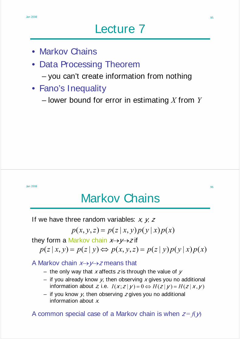
If we have three random variables: x, y, z

)()|(),|(),,( xpxypyxzpzyxp =they form a Markov chain x→y→z if

)()|()|(),,()|(),|( xpxypyzpzyxpyzpyxzp =⇔=

A Markov chain x→y→z means that– the only way that x affects z is through the value of y

),|()|(0)|;( yxzyzyzx HHI =⇔=– if you already know y, then observing x gives you no additional

information about z, i.e.– if you know y, then observing z gives you no additional

information about x.

A common special case of a Markov chain is when z = f(y)

Jan 2008 97

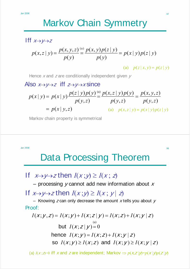
Markov Chain Symmetry

Iff x→y→z

)|()|()(

)|(),(

)(

),,()|,(

)a(

yzpyxpyp

yzpyxp

yp

zyxpyzxp ===

)|(),|((a) yzpyxzp =

Also x→y→z iff z→y→x since

),|(

),(

),,(

),(

)()|,(

),(

)()|()|()|(

(a)

zyxp

zyp

zyxp

zyp

ypyzxp

zyp

ypyzpyxpyxp

=

===

Hence x and z are conditionally independent given y

Markov chain property is symmetrical

)|()|()|,((a) yzpyxpyzxp =

Jan 2008 98

Data Processing Theorem

If x→y→z then I(x ;y) ≥ I(x ; z)– processing y cannot add new information about x

)|;();();(

0)|;((a)

zyxzxyxyzx

III

I

+==

hence

but

(a) I(x ;z)=0 iff x and z are independent; Markov ⇒ p(x,z |y)=p(x |y)p(z |y)

If x→y→z then I(x ;y) ≥ I(x ; y | z)– Knowing z can only decrease the amount x tells you about y

Proof:)|;();()|;();(),;( zyxzxyzxyxzyx IIIII +=+=

)|;();();();( zyxyxzxyx IIII ≥≥ and so

Jan 2008 99

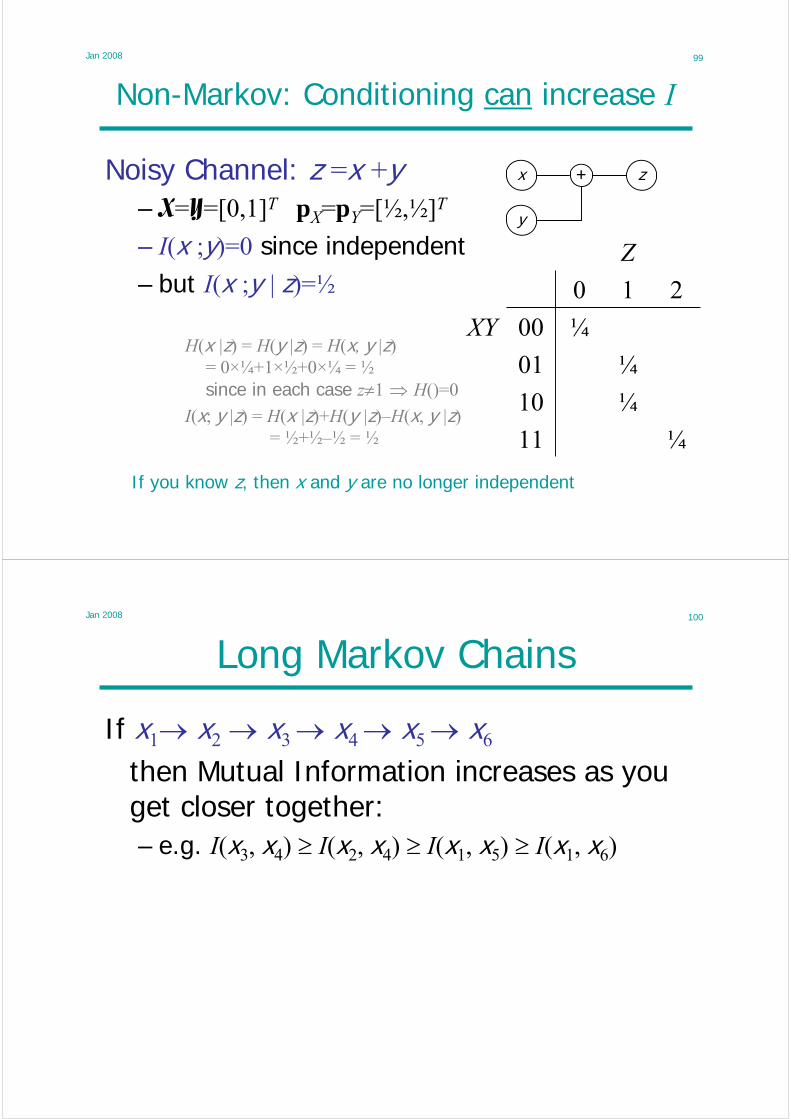
Non-Markov: Conditioning can increase I

Noisy Channel: z =x +y– X=Y=[0,1]T pX=pY=[½,½]T

– I(x ;y)=0 since independent

x z

y

+

¼11

¼10

¼01

¼00XY

210

Z

If you know z, then x and y are no longer independent

H(x |z) = H(y |z) = H(x, y |z) = 0×¼+1×½+0×¼ = ½since in each case z≠1 ⇒ H()=0

I(x; y |z) = H(x |z)+H(y |z)–H(x, y |z)= ½+½–½ = ½

– but I(x ;y | z)=½

Jan 2008 100

Long Markov Chains

If x1→ x2 → x3 → x4 → x5 → x6

then Mutual Information increases as you get closer together:– e.g. I(x3, x4) ≥ I(x2, x4) ≥ I(x1, x5) ≥ I(x1, x6)

Jan 2008 101

Sufficient Statistics

If pdf of x depends on a parameter θ and you extract a statistic T(x) from your observation,then );())(;()( xxxx θθθ ITIT ≤⇒→→

))(|()),(|(

)(

);())(;()(

xxxxxx

xxxx

TpTp

T

ITIT

=⇔→→→⇔

=⇔→→→

θθθ

θθθθ

∑=

=n

iinT

1:1 )( xx ( )

⎪⎩

⎪⎨⎧

≠=

===∑∑∑

−

kx

kxCkxXp

i

ikninn if

if0

,|1

:1:1 xθ

independent of θ ⇒ sufficient

T(x) is sufficient for θ if the stronger condition:

Example: xi ~ Bernoulli(θ ),

Jan 2008 102

Fano’s Inequality

If we estimate x from y, what is ?x xy ^

)ˆ( xx ≠= ppe

( )( )

( )( )

( )1||log

1)|(

1||log

)()|(

1||log)()|((a)

−−

≥−

−≥⇒

−+≤

XX

X

yxyxyx

HpHHp

ppHH

ee

ee

Proof: Define a random variable 0:1?)ˆ( xxe ≠=

eee pppH )1|log(|)1(0)( −+−×+≤ X

(a) the second form is weaker but easier to use

chain rule

H≥0; H(e |y)≤H(e)

H(e)=H(pe)

Fano’s inequality is used whenever you need to show that errors are inevitable

),|()|(),|()|()|,( yexyeyxeyxyxe HHHHH +=+=),|()(0)|( yexeyx HHH +≤+⇒

ee peHpeHH )1,|()1)(0,|()( =+−=+= yxyxe

Jan 2008 103

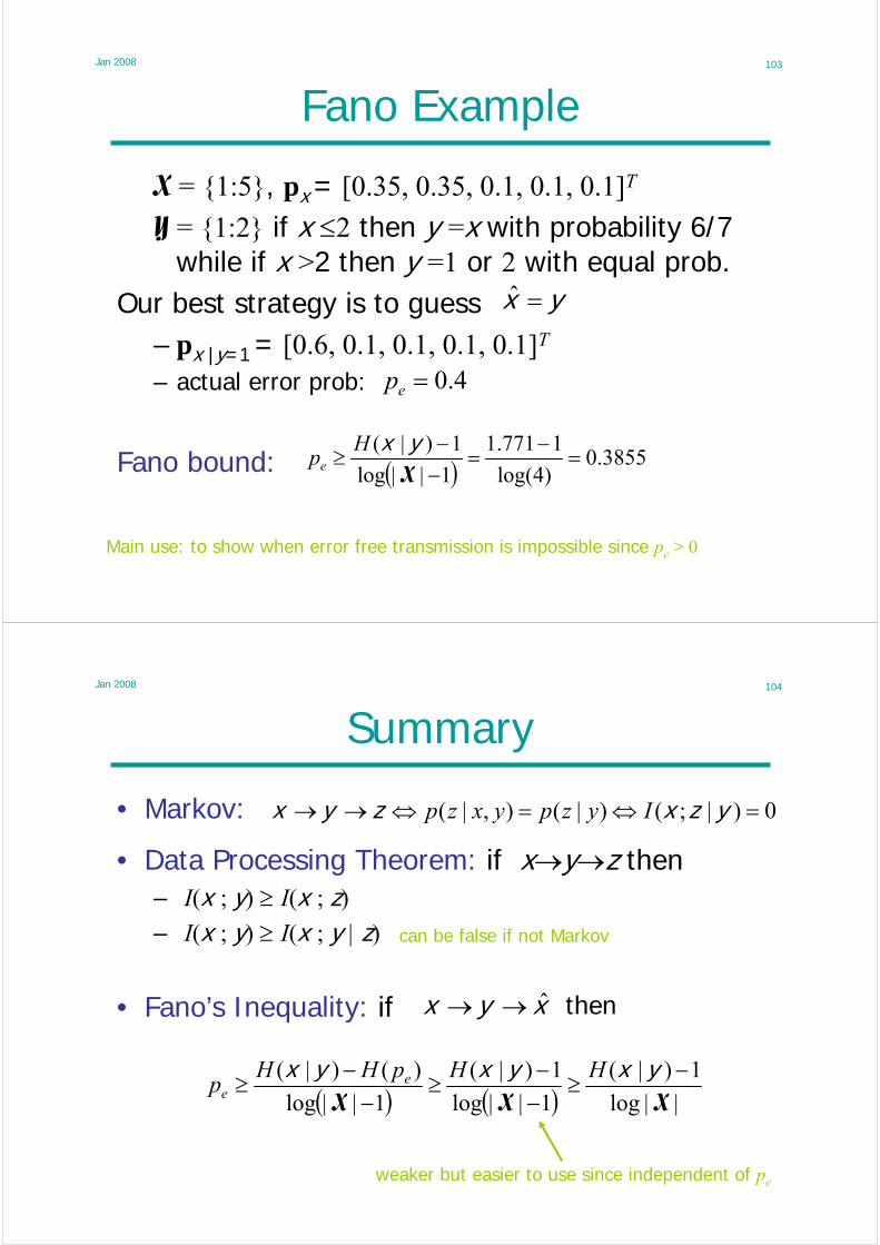
Fano Example

X = {1:5}, px = [0.35, 0.35, 0.1, 0.1, 0.1]T

Y = {1:2} if x ≤2 then y =x with probability 6/7 while if x >2 then y =1 or 2 with equal prob.

Our best strategy is to guess – px |y=1 = [0.6, 0.1, 0.1, 0.1, 0.1]T

– actual error prob:

Fano bound: ( ) 3855.0)4log(

1771.1

1||log

1)|(=

−=

−−

≥XyxH

pe

Main use: to show when error free transmission is impossible since pe > 0

yx =ˆ

4.0=ep

Jan 2008 104

Summary

• Markov:

• Data Processing Theorem: if x→y→z then– I(x ; y) ≥ I(x ; z)

– I(x ; y) ≥ I(x ; y | z)

• Fano’s Inequality: if

can be false if not Markov

then xyx ˆ→→

( ) ( ) ||log

1)|(

1||log

1)|(

1||log

)()|(

XXX−

≥−−

≥−

−≥

yxyxyx HHpHHp e

e

0)|;()|(),|( =⇔=⇔→→ yzxzyx Iyzpyxzp

weaker but easier to use since independent of pe

Jan 2008 105

Lecture 8

• Weak Law of Large Numbers• The Typical Set

– Size and total probability

• Asymptotic Equipartition Principle

Jan 2008 106

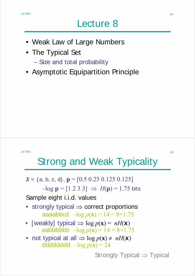
Strong and Weak Typicality

X = {a, b, c, d}, p = [0.5 0.25 0.125 0.125]

–log p = [1 2 3 3] ⇒ H(p) = 1.75 bits

Sample eight i.i.d. values• strongly typical ⇒ correct proportions

aaaabbcd –log p(x) = 14 = 8×1.75• [weakly] typical ⇒ log p(x) = nH(x)

aabbbbbb –log p(x) = 14 = 8×1.75• not typical at all ⇒ log p(x) ≠ nH(x)

dddddddd –log p(x) = 24

Strongly Typical ⇒ Typical

Jan 2008 107

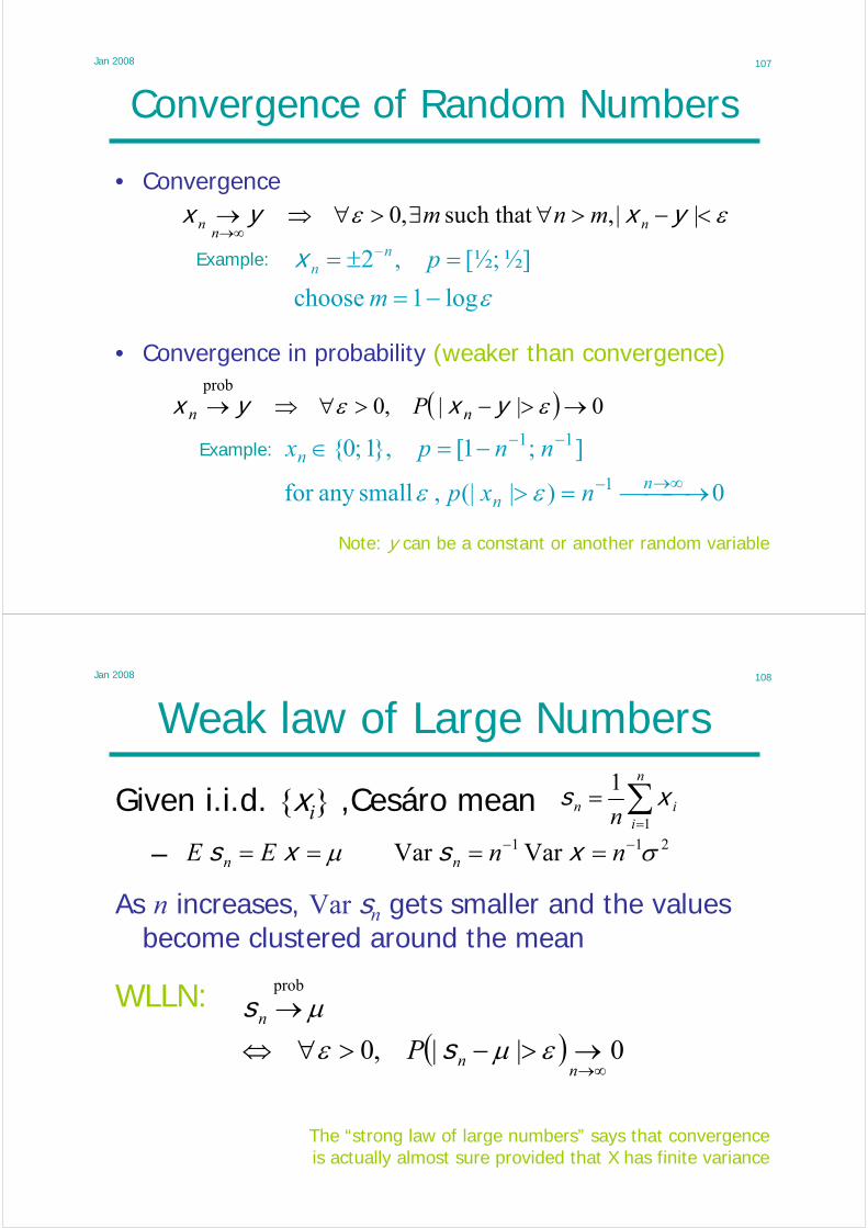
Convergence of Random Numbers

• Convergenceεε <−>∀∃>∀⇒→

∞→||,such that ,0 yxyx n

nn mnm

( ) 0||,0prob

→>−>∀⇒→ εε yxyx nn P

Note: y can be a constant or another random variable

εlog1 choose

½][½;,2–

−==±=

m

pnnxExample:

0)|(| , smallany for

];1[},1;0{1

11

⎯⎯ →⎯=>

−=∈∞→−

−−

nn

n

nxp

nnpx

εε

Example:

• Convergence in probability (weaker than convergence)

Jan 2008 108

Weak law of Large Numbers

Given i.i.d. {xi} ,Cesáro mean

–

As n increases, Var sn gets smaller and the values become clustered around the mean

∑=

=n

iin n 1

1 xs

211 VarVar σμ −− ==== nnEE nn xsxs

( ) 0||,0

prob

∞→→>−>∀⇔

→

nn

n

P εμεμ

ss

The “strong law of large numbers” says that convergence is actually almost sure provided that X has finite variance

WLLN:

Jan 2008 109

Proof of WLLN

• Chebyshev’s Inequality

2

1

Var and where1 σμ === ∑

=ii

n

iin E

nxxxs

( ) ( )

( ) ( )εμεεμ

μμ

εμεμ

>−=≥−≥

−=−=

∑∑

∑

>−>−

∈

ypypypy

ypyE

yyyy

y

2

|:|

2

|:|

2

22

)()(

)(VarY

yy

• WLLN

( ) 0Var2

2

∞→→=≤>−

nnn n

pσεμε ss

μprob

→nsHenceActually true even if σ = ∞

For any choice of ε

Jan 2008 110

Typical Set

xn is the i.i.d. sequence {xi} for 1 ≤ i ≤ n– Prob of a particular sequence is–– Typical set:

Example:– xi Bernoulli with p(xi =1)=p

– e.g. p([0 1 1 0 0 0])=p2(1–p)4

– For p=0.2, H(X)=0.72 bits– Red bar shows T0.1

(n)

∏=

=n

iipp

1

)()( xx

)()(log)(log xnHxpEnpE i =−=− x

{ }εε <−−∈= − )()(log: 1)( xHpnT nn xx X

-2.5 -2 -1.5 -1 -0.5 0

N-1log p(x)

N=1, p=0.2, e=0.1, pT=0%

-2.5 -2 -1.5 -1 -0.5 0

N-1log p(x)

N=2, p=0.2, e=0.1, pT=0%

-2.5 -2 -1.5 -1 -0.5 0

N-1log p(x)

N=4, p=0.2, e=0.1, pT=41%

-2.5 -2 -1.5 -1 -0.5 0

N-1log p(x)

N=8, p=0.2, e=0.1, pT=29%

-2.5 -2 -1.5 -1 -0.5 0

N-1log p(x)

N=16, p=0.2, e=0.1, pT=45%

-2.5 -2 -1.5 -1 -0.5 0

N-1log p(x)

N=32, p=0.2, e=0.1, pT=62%

-2.5 -2 -1.5 -1 -0.5 0

N-1log p(x)

N=64, p=0.2, e=0.1, pT=72%

-2.5 -2 -1.5 -1 -0.5 0

N-1log p(x)

N=128, p=0.2, e=0.1, pT=85%

Jan 2008 111

1111, 1101, 1010, 0100, 000000110011, 00110010, 00010001, 00010000, 000000000010001100010010, 0001001010010000, 0001000100010000, 0000100001000000, 00000000100000001, 011, 10, 00

Typical Set Frames

-2.5 -2 -1.5 -1 -0.5 0

N-1log p(x)

N=1, p=0.2, e=0.1, pT=0%

-2.5 -2 -1.5 -1 -0.5 0

N-1log p(x)

N=2, p=0.2, e=0.1, pT=0%

-2.5 -2 -1.5 -1 -0.5 0

N-1log p(x)

N=4, p=0.2, e=0.1, pT=41%

-2.5 -2 -1.5 -1 -0.5 0

N-1log p(x)

N=8, p=0.2, e=0.1, pT=29%

-2.5 -2 -1.5 -1 -0.5 0

N-1log p(x)

N=16, p=0.2, e=0.1, pT=45%

-2.5 -2 -1.5 -1 -0.5 0

N-1log p(x)

N=32, p=0.2, e=0.1, pT=62%

-2.5 -2 -1.5 -1 -0.5 0

N-1log p(x)

N=64, p=0.2, e=0.1, pT=72%

-2.5 -2 -1.5 -1 -0.5 0

N-1log p(x)

N=128, p=0.2, e=0.1, pT=85%

Jan 2008 112

Typical Set: Properties

1. Individual prob:

2. Total prob:

3. Size:

εε nnHpT n ±−=⇒∈ )()(log)( xxx

εε ε NnTp n >−>∈ for 1)( )(x

εεε εε <>−−>∀∃>∀

=−→−=−

−

=

−− ∑))()(log( s.t. 0 Hence

)()(log)(log)(log

1

prob

1

11

x

x

HpnpNnN

HxpExpnpn i

n

ii

x

x

22)1( ))(()())(( εε

ε ε

ε +>

− ≤<− xx HnnNn

Hn T

)())(())(( 22)()(1)()(

nHn

T

Hn

T

Tppnn

εεε

εε

+−

∈

+−

∈

=≥≥= ∑∑∑ xx

xxx

xx

)())(())(()( 22)(1, f.l.e.)(

nHn

T

Hnn TTpnn

εεε

εε

ε −−

∈

−− =≤∈<− ∑ xx

x

x

Proof 2:

Proof 3a:

Proof 3b:

Jan 2008 113

Asymptotic Equipartition Principle

• for any ε and for n > Nε“Almost all events are almost equally surprising”

• εε −>∈ 1)( )(nTp x and

elements ))((2 ε+≤ xHn

)(nTε∈x)(nTε∉x

( )( )12log

log)(2−+++=

+++≤

nHn

nHn

X

X

εε

εε

εnnHp ±−= )()(log xx

Coding consequence– : ‘0’ + at most 1+n(H+ε) bits – : ‘1’ + at most 1+nlog|X| bits– L = Average code length

|X|n elements

Jan 2008 114

Source Coding & Data Compression

For any choice of δ > 0, we can, by choosing block size, n, large enough, do either of the following:

• make a lossless code using only H(x)+δ bits per symbol on average:

• make a code with an error probability < ε using H(x)+ δbits for each symbol – just code Tε using n(H+ε+n–1) bits and use a random wrong code

if x∉Tε

( )12log −+++≤ nHnL Xεε

Jan 2008 115

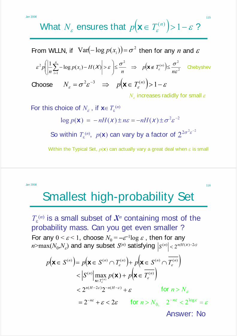
From WLLN, if then for any n and ε( ) 2)(logVar σ=− ixp

( )2

2)(

2

1

2 )()(log1

εσσεε ε n

Tpn

Hxpn

p nn

ii ≤∉⇒≤⎟⎟

⎠

⎞⎜⎜⎝

⎛>−−∑

=

xX

Choose ( ) εεσ εε −>∈⇒= − 1)(32 nTpN x

For this choice of Nε , if x∈Tε(n)

So within Tε(n), p(x) can vary by a factor of

2222−εσ

22)()()(log −±−=±−= εσε xx nHnnHp x

Within the Typical Set, p(x) can actually vary a great deal when ε is small

( ) ? that ensures What εεε −>∈ 1)(nTpN x

εε smallfor radidly increases N

Chebyshev

Jan 2008 116

Smallest high-probability Set

Tε(n) is a small subset of Xn containing most of the

probability mass. Can you get even smaller ?

ε)n(HnS 2)()( 2 −< x

( ) ( ) ( ))()()()()( nnnnn TSpTSpSp εε ∩∈+∩∈=∈ xxx

Answer: No

εεε =<> − log,0 22 nNnfor

εNn >for

For any 0 < ε < 1, choose N0 = –ε–1log ε , then for any n>max(N0,Nε) and any subset S(n) satisfying

( ))()( )(max)(

n

T

n TppSn ε

ε

∈+<∈

xxx

εεε +< −−− )()2( 22 HnHn

εεε 22 <+= −n

Jan 2008 117

Summary

• Typical Set– Individual Prob– Total Prob– Size

• No other high probability set can be much smaller than

• Asymptotic Equipartition Principle– Almost all event sequences are equally surprising



22)1( ))(()())(( εε

ε ε

ε +>


Hn T

)(nTε

Jan 2008 118

Lecture 9

• Source and Channel Coding• Discrete Memoryless Channels

– Symmetric Channels– Channel capacity

• Binary Symmetric Channel• Binary Erasure Channel• Asymmetric Channel

Jan 2008 119

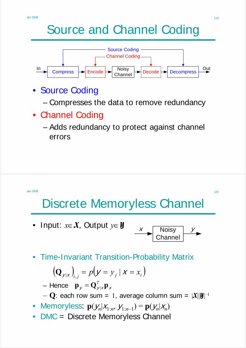
Source and Channel Coding

• Source Coding– Compresses the data to remove redundancy

• Channel Coding– Adds redundancy to protect against channel

errors

Compress DecompressEncode DecodeNoisy

Channel

Source Coding

Channel Coding

In Out

Jan 2008 120

Discrete Memoryless Channel

• Input: x∈X, Output y∈Y

• Time-Invariant Transition-Probability Matrix

– Hence– Q: each row sum = 1, average column sum = |X||Y|–1

• Memoryless: p(yn|x1:n, y1:n–1) = p(yn|xn)• DMC = Discrete Memoryless Channel

( ) ( )ijjixyp === xyxy |

,|Q

xxyy pQp T|=

NoisyChannel

x y

Jan 2008 121

Binary Channels

• Binary Symmetric Channel– X = [0 1], Y = [0 1]

• Binary Erasure Channel– X = [0 1], Y = [0 ? 1]

• Z Channel– X = [0 1], Y = [0 1]

Symmetric: rows are permutations of each other; columns are permutations of each otherWeakly Symmetric: rows are permutations of each other; columns have the same sum

⎟⎟⎠

⎞⎜⎜⎝

⎛−

−ff

ff

1

1

⎟⎟⎠

⎞⎜⎜⎝

⎛−

−ff

ff

10

01

⎟⎟⎠

⎞⎜⎜⎝

⎛− ff 1

01

x0

1

0

1y

x0

1

0

1y

x

0

1

0

? y

1

Jan 2008 122

Weakly Symmetric ChannelsWeakly Symmetric:

1. All columns of Q have the same sum = |X||Y|–1

– If x is uniform (i.e. p(x) = |X|–1) then y is uniform1111

)|()()|()(−−−

∈

−

∈

=×=== ∑∑ YYXXXXX xx

xypxpxypyp

)()()()|()()|( :,1:,1 QQ HxpHxHxpHxx

==== ∑∑∈∈ XX

xyxy

where Q1,: is the entropy of the first (or any other) row of the Q matrix

Symmetric: 1. All rows are permutations of each other2. All columns are permutations of each otherSymmetric ⇒ weakly symmetric

2. All rows are permutations of each other

– Each row of Q has the same entropy so

Jan 2008 123

Channel Capacity

• Capacity of a DMC channel:

– Maximum is over all possible input distributions px

– ∃ only one maximum since I(x ;y) is concave in px for fixed py|x

– We want to find the px that maximizes I(x ;y)

);(max yxx

ICp

=

);(max1

:1:1)(

:1

nnn I

nC

n

yxxp

=

( ) ( )YX log,logmin)(),(min0 ≤≤≤ yx HHC

♦ = proved in two pages time

♦

H(x |y) H(y |x)

H(x ,y)

H(x) H(y)

I(x ;y)• Capacity for n uses of channel:

– Limits on C:

Jan 2008 124

00.2

0.40.6

0.81 0

0.2

0.4

0.6

0.8

1-0.5

0

0.5

1

Channel Error Prob (f)

I(X;Y)

Input Bernoulli Prob (p)

Mutual Information PlotBinary Symmetric ChannelBernoulli Input f

0

1

0

1

yxf

1–f

1–f

1–p

p

)()2(

)|()();(

fHppffH

HHI

−+−=−= yxyyx

Jan 2008 125

Mutual Information Concave in pX

Mutual Information I(x;y) is concave in px for fixed py|x

)|;();()|;();();,( zyxyzxyzyxyzx IIIII +=+=

U

V

X

Z Y

p(Y|X)

1

0

sobut 0),|()|()|;( =−= zxyxyxyz HHI

);()1();( yvyu II λλ −+=

Special Case: y=x ⇒ I(x; x)=H(x) is concave in px= Deterministic

)|;();( zyxyx II ≥)0|;()1()1|;( =−+== zyxzyx II λλ

Proof: Let u and v have prob mass vectors u and v– Define z: bernoulli random variable with p(1) = λ– Let x = u if z=1 and x=v if z=0 ⇒ px=λu+(1–λ)v

Jan 2008 126

Mutual Information Convex in pY|X

Mutual Information I(x ;y) is convex in py|x for fixed px

xvxuxy ||| )1( ppp λλ −+=

)|;();(

);()|;(),;(

yzxyxzxzyxzyx

II

III

+=+=

sobut 0)|;( and 0);( ≥= yzxzx II

)|;();( zyxyx II ≤= Deterministic

Proof (b) define u, v, x etc:–

)0|;()1()1|;( =−+== zyxzyx II λλ);()1();( vxux II λλ −+=

Jan 2008 127

n-use Channel Capacity

We can maximize I(x;y) by maximizing each I(xi;yi)independently and taking xi to be i.i.d.– We will concentrate on maximizing I(x; y) for a single channel use

)|()();( :1:1:1:1:1 nnnnn HHI xyyyx −=For Discrete Memoryless Channel:

with equality if xi are independent ⇒ yi are independent

Chain; Memoryless

ConditioningReducesEntropy

∑∑∑===

=−≤n

iii

n

iii

n

ii IHH

111

);()|()( yxxyy

∑∑==

− −=n

iii

n

iii HH

111:1 )|()|( xyyy

Jan 2008 128

Capacity of Symmetric Channel

∴ Information Capacity of a BSC is 1–H(f)

f

0

1

0

1

yxf

1–f

1–f

)(||log)()()|()();( :,1:,1 QQ HHHHHI −≤−=−= Yyxyyyx

with equality iff input distribution is uniform

If channel is weakly symmetric:

For a binary symmetric channel (BSC):– |Y| = 2

– H(Q1,:) = H(f)

– I(x;y) ≤ 1 – H(f)

∴ Information Capacity of a WS channel is log|y|–H(Q1,:)

Jan 2008 129

Binary Erasure Channel (BEC)

since a fraction f of the bits are lost, the capacity is only 1–fand this is achieved when x is uniform

x

0

1

0

? y

1

f

f

1–f

1–f)|()();( yxxyx HHI −=

⎟⎟⎠

⎞⎜⎜⎝

⎛−

−ff

ff

10

01

since max value of H(x) = 1with equality when x is uniform

H(x |y) = 0 when y=0 or y=1fHH )()( xx −=

0)1()(?)(0)0()( ×=−=−×=−= yxyyx pHppH

f−≤1

)()1( xHf−=

Jan 2008 130

Asymmetric Channel Capacity

Let px = [a a 1–2a]T ⇒ py=QTpx = pxf

0: a

1: a

0

1 yxf

1–f

1–f

2: 1–2a 2

⎟⎟⎟

⎠

⎞

⎜⎜⎜

⎝

⎛−

−=

100

01

01

ff

ff

Q

To find C, maximize I(x ;y) = H(y) – H(y |x)

( ) ( ) )(221log21log2 faHaaaaI −−−−−=

Note:d(log x) = x–1 log e

Examples: f = 0 ⇒ H(f) = 0 ⇒ a = 1/3 ⇒ C = log 3 = 1.585 bits/usef = ½ ⇒ H(f) = 1 ⇒ a = ¼ ⇒ C = log 2 = 1 bits/use

( ) ( ))(2)1()21()(2)|(

21log21log2)(

faHHafaHH

aaaaH

=−+=−−−−=

xyy

( ) ( ) ( )aaaaC fH 21log212log2 )( −−−−=⇒

0)(2)21log(2log2log2log2 =−−++−−= fHaeaeda

dI

( ) )(2log21

log 1 fHaa

a=−=

− − ( ) 1)(22−

+=⇒ fHa

( )a21log −−=

Jan 2008 131

Lecture 10

• Jointly Typical Sets• Joint AEP• Channel Coding Theorem

– Random Coding– Jointly typical decoding

Jan 2008 132

Significance of Mutual Information

– An average input sequence x1:n corresponds to about 2nH(y|x)

typical output sequences– There are a total of 2nH(y) typical output sequences– For nearly error free transmission, we select a number of input

sequences whose corresponding sets of output sequences hardly overlap

– The maximum number of distinct sets of output sequences is2n(H(y)–H(y|x)) = 2nI(y ;x)

NoisyChannel

x1:n y1:n

2nH(x) 2nH(y|x)

2nH(y)

• Consider blocks of n symbols:

Channel Coding Theorem: for large n can transmit at any rate < C with negligible errors

Jan 2008 133

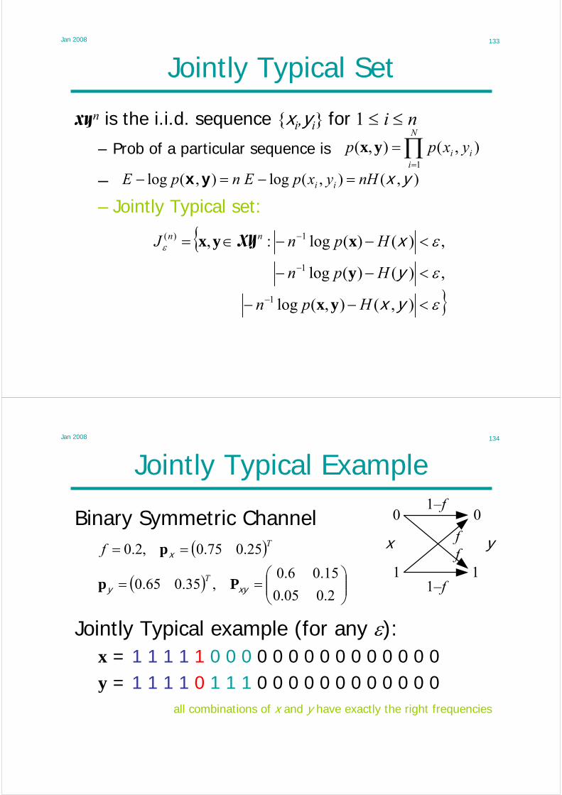
Jointly Typical Set

xyn is the i.i.d. sequence {xi,yi} for 1 ≤ i ≤ n

– Prob of a particular sequence is

–– Jointly Typical set:

∏=

=N

iii yxpp

1

),(),( yx

),(),(log),(log yxnHyxpEnpE ii =−=− yx

{

}εε

εε

<−−

<−−

<−−∈=

−

−

−

),(),(log

,)()(log

,)()(log:,

1

1

1)(

yx

y

x

Hpn

Hpn

HpnJ nn

yx

y

xyx XY

Jan 2008 134

Jointly Typical Example

Binary Symmetric Channelf

0

1

0

1

yxf

1–f

1–f

( )

( ) ⎟⎟⎠

⎞⎜⎜⎝

⎛==

==

2.005.0

15.06.0,35.065.0

25.075.0,2.0

xyy

x

Pp

p

T

Tf

Jointly Typical example (for any ε):x = 1 1 1 1 1 0 0 0 0 0 0 0 0 0 0 0 0 0 0 0y = 1 1 1 1 0 1 1 1 0 0 0 0 0 0 0 0 0 0 0 0

all combinations of x and y have exactly the right frequencies

Jan 2008 135

Jointly Typical DiagramDots represent jointly typical pairs (x,y)

Inner rectangle represents pairs that are typical in x or y but not necessarily jointly typical

2nlog|X| 2nH(x)

2nlog|Y|

2nH(Y)

2nH(y|x)

2nH(x|y)

Typical in both x, y: 2n(H(x)+H(y))

All sequences: 2nlog(|X||Y|)

Jointly typical: 2nH(x,y)

• There are about 2nH(x) typical x’s in all• Each typical y is jointly typical with about 2nH(x|y) of these typical x’s• The jointly typical pairs are a fraction 2–nI(x ;y) of the inner rectangle • Channel Code: choose x’s whose J.T. y’s don’t overlap; use J.T. for decoding

Each point defines both an x sequence and a y sequence

Jan 2008 136

Joint Typical Set Properties

1. Indiv Prob:2. Total Prob: 3. Size:

( ) εε ε NnJp n >−>∈ for1, )(yx( ) ( )ε

εε ε

ε +>

− ≤<− ),()(),( 22)1( yxyx HnnNn

Hn J

Proof 2: (use weak law of large numbers)

( )( )32132

111

,,max,3

)()(log,

NNNNNN

HpnpNnN

=

<>−−>∀ −

ε

εε

set and conditionsother for chooseSimilarly

that such Choose xx

( ) εε nnHpJ n ±−=⇒∈ ),(,log, )( yxyxyx

( )εεε

εε

ε −−

∈∈

=≤<− ∑ ),()(

,

)(

,

2),(max),(1)(

)(

yxHnn

J

n

J

JpJpn

n

yxyxyx

yx

∀n

n>NεProof 3:

( )εεε

εε

+−

∈∈

=≥≥ ∑ ),()(

,

)(

,

2),(min),(1)(

)(

yxHnn

J

n

J

JpJpn

n

yxyxyx

yx

Jan 2008 137

Joint AEP

If px'=px and py' =py with x' and y' independent:( ) ( ) ( )

εε

εεε NnJp InnIn >≤∈≤− −−+− for 3),()(3),( 2','2)1( yxyx yx

Proof: |J| × (Min Prob) ≤ Total Prob ≤ |J| × (Max Prob)

( )( )

εε

εε

εε

Nn

ppJJp

In

J

nn

n

>−≥

≥∈

+−

∈

for 3);(

','

)()(

2)1(

)'()'(min',')(

y x

yxyxyx

( ) ∑∑∈∈

==∈)()( ','','

)( )'()'()','(','nn JJ

n pppJpεε

εyxyx

yxyxyx

( )( ) ( ) ( ) ( )εεεε

εεε

3);()()(),(

','

)()(

2222

)'()'(max',')(

−−−−−−+

∈

=≤

≤∈

y xyxyx InHnHnHn

J

nn ppJJpn

yxyxyx

Jan 2008 138

Channel Codes

• Assume Discrete Memoryless Channel with known Qy|x

• An (M,n) code is– A fixed set of M codewords x(w)∈Xn for w=1:M

– A deterministic decoder g(y)∈1:M

( )( )( ) ( )∑∈

≠=≠=n

wgw wpwwgpYy

yxy )()(| δλ y

∑=

=M

ww

ne M

P1

)( 1 λ

wMw

n λλ≤≤

=1

)( max

δC = 1 if C is true or 0 if it is false

• Error probability

– Maximum Error Probability

– Average Error probability

Jan 2008 139

Achievable Code Rates

• The rate of an (M,n) code: R=(log M)/n bits/transmission• A rate, R, is achievable if

– ∃ a sequence of codes for n=1,2,…

– max prob of error λ(n)→0 as n→∞– Note: we will normally write to mean

⎡ ⎤( )nnR ,2

( )nnR ,2 ⎡ ⎤( )nnR ,2

• The capacity of a DMC is the sup of all achievable rates

• Max error probability for a code is hard to determine– Shannon’s idea: consider a randomly chosen code– show the expected average error probability is small– Show this means ∃ at least one code with small max error prob– Sadly it doesn’t tell you how to find the code

Jan 2008 140

Channel Coding Theorem

• A rate R is achievable if R<C and not achievable if R>C– If R<C, ∃ a sequence of (2nR,n) codes with max prob of error

λ(n)→0 as n→∞– Any sequence of (2nR,n) codes with max prob of error λ(n)→0 as

n→∞ must have R ≤ C

0 1 2 30

0.05

0.1

0.15

0.2

Rate R/C

Bit

err

or

pro

ba

bili

ty Achievable

Impossible

A very counterintuitive result:Despite channel errors you can get arbitrarily low bit error rates provided that R<C

Jan 2008 141

Lecture 11

• Channel Coding Theorem

Jan 2008 142

Channel Coding Principle

– An average input sequence x1:n corresponds to about 2nH(y|x) typical output sequences

NoisyChannel

x1:n y1:n

2nH(x) 2nH(y|x)

2nH(y)

• Consider blocks of n symbols:

Channel Coding Theorem: for large n, can transmit at any rate R < C with negligible errors

– Random Codes: Choose 2nR random code vectors x(w)• their typical output sequences are unlikely to overlap much.

– Joint Typical Decoding: A received vector y is very likely to be in the typical output set of the transmitted x(w) and no others. Decode as this w.

Jan 2008 143

Random (2nR,n) Code• Choose ε ≈ error prob, joint typicality ⇒ Nε , choose n>Nε

( ) ∑ ∑=

−=C

CCEnR

ww

nRpp2

1

)(2)( λ

(a) since error averaged over all possible codes is independent of w

• Choose px so that I(x ;y)=C, the information capacity

• Use px to choose a code C with random x(w)∈Xn, w=1:2nR

– the receiver knows this code and also the transition matrix Q

• Assume (for now) the message W∈1:2nR is uniformly distributed

• If received value is y; decode the message by seeing how many x(w)’s are jointly typical with y– if x(k) is the only one then k is the decoded message– if there are 0 or ≥2 possible k’s then 1 is the decoded message– we calculate error probability averaged over all C and all W

∑∑=

−=nR

ww

nR p2

1

)()(2 CCC

λ )()( 1

)(

CCC

λ∑= pa

( )1| == wEp

Jan 2008 144

Channel Coding Principle

{ } nRnw wJw 2:1),( )( ∈∈= for εyxe

NoisyChannel

x1:n y1:n

• Assume we transmit x(1) and receive y

• Define the events

• We have an error if either e1 false or ew true for w ≥ 2

• The x(w) for w ≠ 1 are independent of x(1) and hence also

independent of y. So ( ) 1any for 2) true( 3),( ≠< −− wep Inw

εyx Joint AEP

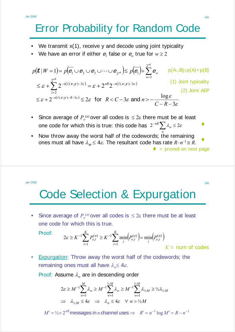
Jan 2008 145

Error Probability for Random Code• We transmit x(1), receive y and decode using joint typicality• We have an error if either e1 false or ew true for w ≥ 2

( ) ( ) ( ) ∑=

+≤∪∪∪∪==nR

nR

wwppWp

2

2123211| eeeeeeE

• Since average of Pe(n) over all codes is ≤ 2ε there must be at least

one code for which this is true: this code has ελ 22 ≤∑−

ww

nR

• Now throw away the worst half of the codewords; the remaining ones must all have λw ≤ 4ε. The resultant code has rate R–n–1 ≅ R.

♦ = proved on next page

♦

♦

(1) Joint typicality

(2) Joint AEP

p(A∪B)≤p(A)+p(B)

( ) ( )εε εε 3);(2

2

3);( 222 −−

=

−− +=+≤ ∑ yxyx InnR

i

In

nR

( )

εεεεε ε

3

log322 3);(

−−−>−<≤+≤ −−−

RCnCRRIn and for yx

Jan 2008 146

Code Selection & Expurgation


one code for which this is true.

Mw

MMM

wM

M

M

wM

M

ww

M

ww

½44

½2

½

½

½

1½

1½

1

1

1

1

>∀≤⇒≤⇒

≥≥≥≥ ∑∑∑=

−

=

−

=

−

ελελ

λλλλε

( ) ( ))(,

1

)(,

1

1

)(,

1 minmin2 nie

i

K

i

nie

i

K

i

nie PPKPK =≥≥ ∑∑

=

−

=

−ε

11 log 2½ −− −=′=′⇒×=′ nRMnRnM nR uses channelin messages

K = num of codes

Proof:

• Expurgation: Throw away the worst half of the codewords; the remaining ones must all have λw≤ 4ε.

Proof: Assume λw are in descending order

Jan 2008 147

Summary of Procedure• Given R´<C, choose ε<¼(C–R´) and set R=R´+ε ⇒ R<C – 3ε

{ }1),3/()(log,max −−−−= εεεε RCNn see (a),(b),(c) below

(a)

(b)

(c)

Note: ε determines both error probability and closeness to capacity

• Set

• Find the optimum pX so that I(x ; y) = C

• Choosing codewords randomly (using pX) and using joint typicality as the decoder, construct codes with 2nR codewords


one code for which this is true. Find it by exhaustive search.

• Throw away the worst half of the codewords. Now the worst codeword has an error prob ≤ 4ε with rate R´ = R – n–1 > R – ε

• The resultant code transmits at a rate R´ with an error probability that can be made as small as desired (but n unnecessarily large).

• The resultant code transmits at a rate R´ with an error probability that can be made as small as desired (but n unnecessarily large).

Jan 2008 148

Lecture 12

• Converse of Channel Coding Theorem– Cannot achieve R>C– Minimum bit-error rate

• Capacity with feedback– no gain but simpler encode/decode

• Joint Source-Channel Coding– No point for a DMC

Jan 2008 149

Converse of Coding Theorem• Fano’s Inequality: if Pe

(n) is error prob when estimating w from y,)()( 1log1)|( n

en

e nRPPH +=+≤ Wyw

• Hence );()|()( yy www IHHnR +==

• Hence for large n, Pe(n) has a lower bound of (R–C)/R if w equiprobable

– If R>C was achievable for small n, it could be achieved also for large n by concatenation. Hence it cannot be achieved for any n.

n-use DMC capacity

Fano

ww ˆ→→→ yx :Markov

Definition of I

));(()|( yxy ww IH +≤

);(1 )( yxInRP ne ++≤

nCnRP ne ++≤ )(1

R

CR

R

nCRP

n

ne

−→

−−≥⇒

∞→

−1)(

Jan 2008 150

Minimum Bit-error Rate

Suppose– v1:nR is i.i.d. bits with H(vi)=1

– The bit-error rate is { } { })()ˆ( ii

iii

b pEpEP evvΔ

=≠=

);( :1:1 nnInC yx(a)

≥

Hence( ) 1)(1 −−≤ bPHCR

(a) n-use capacity

0 1 2 30

0.05

0.1

0.15

0.2

Rate R/C

Bit

err

or

pro

ba

bili

ty

iii vve ˆ⊕=

)ˆ;( :1:1 nRnRI vv(b)

≥ )ˆ|()( :1:1:1 nRnRnR HH vvv −=

∑=

−−=nR

iinRiHnR

11:1:1 ),ˆ|( vvv ∑

=

−≥nR

iiiHnR

1

)ˆ|( vv(c) { }( ))ˆ|(1 ii

iHEnR vv−=

{ }( ))ˆ|(1 iii

HEnR ve−=(d)

{ }( ))(1 ii

HEnR e−≥(c) ( ))(1 bPHnR −=

(b) Data processing theorem(c) Conditioning reduces entropy

(d)

Then

)/1(1 RCHPb −≥ −

( ))(1 ,ibi

PEHnR −≥(e)

(e) Jensen: E H(x) ≤ H(E x)

Jan 2008 151

Channel with Feedback

• Assume error-free feedback: does it increase capacity ?• A (2nR,n) feedback code is

– A sequence of mappings xi = xi(w,y1:i–1) for i=1:n

– A decoding function

NoisyChannel

xi yiEncoder

w∈1:2nR

Decoderw

y1:i–1

)(ˆ:1 ng yw =

0)ˆ()( ⎯⎯ →⎯≠= ∞→nn

e PP ww• A rate R is achievable if ∃ a sequence of (2nR,n) feedback

codes such that

• Feedback capacity, CFB≥C, is the sup of achievable rates

Jan 2008 152

Capacity with Feedback

);()|()( yy www IHHnR +==

)|()();( ww yyy HHI −=

Hence

since xi=xi(w,y1:i–1)

since yi only directly depends on xi

The DMC does not benefit from feedback: CFB = C

cond reduces ent

Fano

NoisyChannel

xi yiEncoder

w∈1:2nR

Decoderw

y1:i–1

∑=

−−=n

iiiHH

11:1 ),|()( wyyy

∑=

−−=n

iiiiHH

11:1 ),,|()( xwyyy

∑=

−=n

iiiHH

1

)|()( xyy

∑∑==

−≤n

iii

n

ii HH

11

)|()( xyy nCIn

iii ≤=∑

=1

);( yx

nCnRP ne ++≤ )(1

R

nCRP n

e

1)(

−−−≥⇒

Jan 2008 153

Example: BEC with feedback

• Capacity is 1–f• Encode algorithm

– If yi=?, retransmit bit i– Average number of transmissions per bit:

x

0

1

0

? y

1

f

f

1–f

1–f

fff

−=+++

1

11 2

• Average number of bits per transmission = 1–f

• Capacity unchanged but encode/decode algorithm much simpler.

Jan 2008 154

Joint Source-Channel Coding

• Assume vi satisfies AEP and |V|<∞– Examples: i.i.d.; markov; stationary ergodic

• Capacity of DMC channel is C– if time-varying:

NoisyChannel

x1:n y1:nEncoder

v1:nDecoder

^v1:n

0)ˆ( :1:1)( ⎯⎯ →⎯≠= ∞→nnn

ne PP vv

);(lim 1 yxInCn

−

∞→=

♦ = proved on next page

♦• Joint Source Channel Coding Theorem:∃ codes with iff H(V) < C– errors arise from incorrect (i) encoding of V or (ii) decoding of Y

• Important result: source coding and channel coding might as well be done separately since same capacity

Jan 2008 155

Source-Channel Proof (⇐)

• For n>Nε there are only 2n(H(V)+ε) v’s in the typical set: encode using n(H(V)+ε) bits– encoder error < ε

• Transmit with error prob less than ε so long as H(V)+ ε < C

• Total error prob < 2ε

Jan 2008 156

Source-Channel Proof (⇒)

Fano’s Inequality: Vlog1)ˆ|( )( nPH ne+≤vv

)()( :11

nHnH v−≤V entropy rate of stationary process

definition of I

Fano + Data Proc Inequ

Memoryless channel

Let CHPn ne ≤⇒→⇒∞→ )(0)( V

NoisyChannel

x1:n y1:nEncoder

v1:nDecoder

^v1:n

)ˆ;()ˆ|( :1:11

:1:11

nnnn InHn vvvv −− +=

( ) );(log1 :1:11)(1

nnn

e InnPn yx−− ++≤ V

CPn ne ++≤ − Vlog)(1

Jan 2008 157

Separation Theorem

• For a (time-varying) DMC we can design the source encoder and the channel coder separately and still get optimum performance

• Not true for– Correlated Channel and Source– Multiple access with correlated sources

• Multiple sources transmitting to a single receiver

– Broadcasting channels• one source transmitting possibly different information to

multiple receivers

Jan 2008 158

Lecture 13

• Continuous Random Variables• Differential Entropy

– can be negative– not a measure of the information in x– coordinate-dependent

• Maximum entropy distributions– Uniform over a finite range– Gaussian if a constant variance

Jan 2008 159

Continuous Random VariablesChanging Variables• pdf: CDF:)(xfx ∫ ∞−

=x

dttfxF )()( xx

)()( 1 yxxy −=⇔= gg

( ) ( ))(1)()( 11 ygFygFyF −− −= xxy or

xxFxxf 5.0)()2,0(5.0)( =⇒∈= xx for

)8,0(125.025.05.0)(25.04 ∈=×=⇒=⇒= yyf foryyxxy

)16,0(125.0¼5.0)( ¾¾¼4 ∈=×=⇒=⇒= −− zzzzf forzzxxz

(a)

(b)

Suppose

according to slope of g(x)

( ) ( ) )()(

)()(

)( 11

1 ygxdy

dxxf

dy

ydgygf

dy

ydFyf Y −

−− ==== wherexxy

• Examples:

• For g(x) monotonic:

Jan 2008 160

Joint Distributions Distributions

Joint pdf:Marginal pdf:Independence:Conditional pdf:

),(, yxf yx

∫∞

∞−= dyyxfxf ),()( ,yxx

)(

),()( ,

| yf

yxfxf

y

yxyx =

)()(),(, yfxfyxf yxyx =⇔

fX

x f Y

y

x

y

)1,(),1,0(1, +∈∈= yyxyf for yx

Example:

)1,(1| +∈= yyxf for yx

( ))1,min(),1,0max()1,min(

1| xxy

xxf −∈

−= for xy

Jan 2008 161

Quantised Random Variables

• Given a continuous pdf f(x), we divide the range of x into bins of width Δ– For each i, ∃xi with

• Define a discrete random variable Y– Y = {xi} and py = {f(xi)Δ}

– Scaled,quantised version of f(x) with slightly unevenly spaced xi

∫Δ+

Δ=Δ

)1()()(

i

ii dxxfxf

( )( )

)(log)(log)(log

)(log)(log

)(log)()(

0x

y

hdxxfxf

xfxf

xfxfH

ii

ii

+Δ−=−Δ−→

Δ−Δ−=

ΔΔ−=

∫∑

∑

∞

∞−→Δ

∫∞

∞−−= dxxfxfh )(log)()( xxx

mean value theorem

• Differential entropy:

•

Jan 2008 162

Differential Entropy

Differential Entropy: )(log)(log)()( xfEdxxfxfh xxxx −=−= ∫∞

∞−

Δ

Good News:– h1(x)–h2(x) does compare the uncertainty of two continuous

random variables provided they are quantised to the same precision

– Relative Entropy and Mutual Information still work fine– If the range of x is normalized to 1 and then x is quantised to n

bits, the entropy of the resultant discrete random variable is approximately h(x)+n

Bad News:– h(x) does not give the amount of information in x– h(x) is not necessarily positive– h(x) changes with a change of coordinate system

Jan 2008 163

Differential Entropy Examples

• Uniform Distribution:–

–

– Note that h(x) < 0 if (b–a) < 1

),(~ baUx

elsewhere and for 0)(),()()( 1 =∈−= − xfbaxabxf

)log()(log)()( 11 abdxababhb

a−=−−−= −−∫x

),(~ 2σμNx( ) ( )22½2 )½(exp2)( −−

−−= σμπσ xxf

∫∞

∞−−= dxxfxfeh )(ln)()(log)(x

• Gaussian Distribution:–

–

( )∫∞

∞−

−−−−−= 222 )½()2ln(½)()(log σμπσ xxfe

( ) bits e )1.4log(2log½ 2 σσπ ≅=

( )( )222 )()2ln()½(log μσπσ −+= − xEe

( )1)2ln()½(log 2 += πσe

Jan 2008 164

Multivariate GaussianGiven mean, m, and symmetric +ve definite covariance matrix K,

( ))()½(exp2)(),(~ 1½

:1 mxKmxKxKmN −−−=⇔ −− Tn f πx

( ) ( ) xKmxKmxx dfefh T∫ −−−−×−= − π2ln½)()½()(log)( 1

( ) ( )( ))()(2lnlog½ 1 mxKmxK −−+×= −TEe π

( ) ( )( )1))((tr2lnlog½ −−−+×= KmxmxK TEe π

( ) ( )( )1tr2lnlog½ −+×= KKKπe ( ) ( )ne +×= Kπ2lnlog½

( ) ( )Kπ2log½log½ += ne

( ) bitsKeπ2log½=

( ) ( )( )1))((tr2lnlog½ −−−+×= KmxmxK TEe π

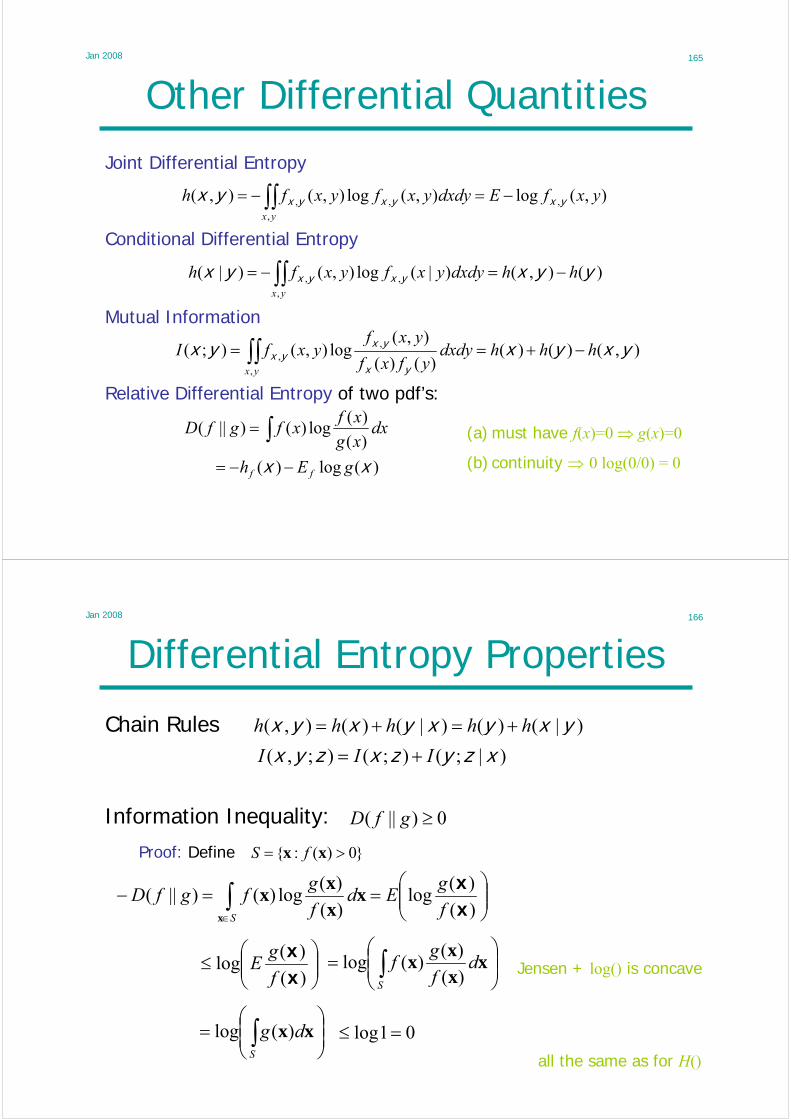
Jan 2008 165

Other Differential QuantitiesJoint Differential Entropy

),(log),(log),(),( ,

,

,, yxfEdxdyyxfyxfhyx

yxyxyxyx −=−= ∫∫

)(),()|(log),()|(,

,, yyxyx yxyx hhdxdyyxfyxfhyx

−=−= ∫∫

)(log)(

)(

)(log)()||(

xx gEh

dxxg

xfxfgfD

ff −−=

= ∫

),()()()()(

),(log),();(

,

,, yxyxyx

yx

yxyx hhhdxdy

yfxf

yxfyxfI

yx

−+== ∫∫

(a) must have f(x)=0 ⇒ g(x)=0

(b) continuity ⇒ 0 log(0/0) = 0

Relative Differential Entropy of two pdf’s:

Mutual Information

Conditional Differential Entropy

Jan 2008 166

Differential Entropy Properties

Chain Rules )|()()|()(),( yxyxyxyx hhhhh +=+=

)|;();();,( xzyzxzyx III +=

0)||( ≥gfD

⎟⎟⎠

⎞⎜⎜⎝

⎛==− ∫

∈ )(

)(log

)(

)(log)()||(

xx

f

gEd

f

gfgfD

Sx

xx

xx

Proof: Define }0)(:{ >= xx fS

Jensen + log() is concave

all the same as for H()

Information Inequality:

⎟⎟⎠

⎞⎜⎜⎝

⎛≤

)(

)(log

xx

f

gE ⎟⎟

⎠

⎞⎜⎜⎝

⎛= ∫

S

df

gf x

x

xx

)(

)()(log

⎟⎟⎠

⎞⎜⎜⎝

⎛= ∫

S

dg xx)(log 01log =≤

Jan 2008 167

Information Inequality Corollaries

Mutual Information ≥ 0

0)||();( , ≥= yxyxyx fffDI

0);()|()( ≥=− yxyxx Ihh

∑∑==

− ≤=n

ii

n

iiin hhh

111:1:1 )()|()( xxxx

all the same as for H()

Independence Bound

Conditioning reduces Entropy

Jan 2008 168

Change of Variable

Change Variable: )(xy g=

( )dy

ydgygfyf

)()()(

11

−−= xyfrom earlier

))(log()( yy yfEh −=

Examples:– Translation: )()(1/ xyxy hhdxdya =⇒=⇒+=

1log)()(/ −−=⇒=⇒= chhcdxdyc xyxy

not the same as for H()

)det(log)()(:1:1 AA +=⇒= xy hhnn xy

( )dy

dxEfE log)(log −−= xx

( )dy

dxEgfE log))((log 1 −−= − yx

dy

dxEh log)( −= x

– Vector version:

– Scaling:

Jan 2008 169

Concavity & Convexity• Differential Entropy:

– h(x) is a concave function of fx(x) ⇒ ∃ a maximum• Mutual Information:

– I(x ; y) is a concave function of fx (x) for fixed fy|x (y)

– I(x ; y) is a convex function of fy|x (y) for fixed fx (x)

U

VX

Z

1

0

U

VX

Z Y

f(y|x)

1

0

U

VY

Z

f(u|x)

X

f(v|x)

1

0

)|()( zxx HH ≥ )()( zyxyx |;I;I ≥ )()( zyxyx |;I;I ≤

Proofs:Exactly the same as for the discrete case: pz = [1–λ, λ]T

Jan 2008 170

Uniform Distribution Entropy

What distribution over the finite range (a,b) maximizes the entropy ?

Answer: A uniform distribution u(x)=(b–a)–1

)||(0 ufD≤

Proof:Suppose f(x) is a distribution for x∈(a,b)

)(log)( xx uEh ff −−=

)log()( abhf −≤⇒ x

)log()( abhf −+−= x

Jan 2008 171

Maximum Entropy Distribution

What zero-mean distribution maximizes the entropy on(–∞, ∞)n for a given covariance matrix K ?

Answer: A multivariate Gaussian ( )xKxKx 1½½exp2)( −−

−= Tπφ

)(log)()||(0 xx φφ ff EhfD −−=≤

Since translation doesn’t affect h(X), we can assume zero-mean w.l.o.g.

EfxxT = K

tr(I)=n=ln(en)

Proof:

( )Keπ2log½=

( ) ( )( )xxx 1½2ln½log)( −−−−≤⇒ KK Tff Eeh π

( ) ( ) ( )( )1tr2lnlog½ −+= KK TfEe xxπ

( ) ( ) ( )( )IK tr2lnlog½ += πe

)(xφh=

Jan 2008 172

Lecture 14

• Discrete-time Gaussian Channel Capacity– Sphere packing

• Continuous Typical Set and AEP• Gaussian Channel Coding Theorem• Bandlimited Gaussian Channel

– Shannon Capacity– Channel Codes

Jan 2008 173

Capacity of Gaussian ChannelDiscrete-time channel: yi = xi + zi

– Zero-mean Gaussian i.i.d. zi ~ N(0,N)

– Average power constraint+

Xi Yi

Zi

Pxnn

ii ≤∑

=

−

1

21

);(max2

yxx

ICPE ≤

=

)|()( xzxy +−= hh

(a) Translation independence

NPEEEEEE +≤++=+= 2222 )()(2)( zzxxzxy X,Z indep and EZ=0

Gaussian Limit withequality when x~N(0,P)

The optimal input is Gaussian & the worst noise is Gaussian

Information Capacity

– Define information capacity:

)|()();( xyyyx hhI −=

)|()()(

xzy hha

−=

( )11log½ −+= PN

)()( zy hh −=

( ) eNNPe ππ 2log½2log½ −+≤

[ ]dB6

1N

NP+=

Jan 2008 174

Gaussian Channel Code Rate

• An (M,n) code for a Gaussian Channel with power constraint is– A set of M codewords x(w)∈Xn for w=1:M with x(w)Tx(w) ≤ nP ∀w

– A deterministic decoder g(y)∈0:M where 0 denotes failure– Errors: )()( n

ei

n

ii P:average :max :codeword λλ

0)(

∞→→

n

nλ

( )11log½ −+=< PNCR

+

z

Encoder Decoderx yw∈1:2nR w∈0:2nR

^

♦ = proved on next pages

♦• Theorem: R achievable iff

• Rate R is achievable if ∃ seq of (2nR,n) codes with

Jan 2008 175

• Volume of hypersphere• Max number of non-overlapping clouds:

Sphere Packing• Each transmitted xi is received as a

probabilistic cloud yi

– cloud ‘radius’ = ( ) nN=xy |Var

( )NPn +

nr∝

( )( )11log½

½

½

2)( −+=

+ PNnn

n

nN

nNnP

• Max rate is ½log(1+PN–1)

• Energy of yi constrained to n(P+N) so clouds must fit into a hypersphere of radius

Jan 2008 176

Continuous AEPTypical Set: Continuous distribution, discrete time i.i.d.

For any ε>0 and any n, the typical set with respect to f(x) is

{ }εε ≤−−∈= − )()(log: 1)( xhfnST nn xx

)(log)(log)(

)()(

1

1

xfEnfEh

xxffn

iii

−

=

−=−=

=∏xx

tindependen are since x


))(()())(( 2)Vol(2)1( εε

ε ε

ε +>

− ≤≤− xx hnnNn

hn T

Proof: WLLN

Proof: Integrate max/min prob

∫∈

=A

dAx

x)Vol( where

Typical Set Properties1.

where S is the support of f ⇔ {x : f(x)>0}

2.

Jan 2008 177

Continuous AEP Proof

Proof 1: By weak law of large numbers)()(log)(log)(log

1

1:1

1 xxxx hfEfnfnprobn

iin =−→−=− ∑

=

−−

( ) εεε εε <>−>∀∃>∀⇒→ ||,,0prob

yxyx nn PNnN that such

( ) ( ) ( ))()()( Vol22)(

nXhn

T

Xhn Tdn

εεε

ε

−−−− =≤ ∫ x

∫∫ ≥=)(

)()(1nn TS

dfdfε

xxxx

max f(x) within T

Property 1

min f(x) within T

Proof 2b:

Proof 2a:

Reminder:

ε

ε

ε NndfnT

>≤− ∫ for )(

)(1 xx

( ) ( ) ( ))()()( Vol22)(

nXhn

T

Xhn Tdn

εεε

ε

+−+− =≥ ∫ x

Jan 2008 178

Jointly Typical SetJointly Typical: xi,yi i.i.d from ℜ2 with fx,y (xi,yi)

{

}εε

εε

<−−

<−−

<−−ℜ∈=

−

−

−

),(),(log

,)()(log

,)()(log:,

,1

1

12)(

yx

y

x

hfn

hfn

hfnJ

YX

Y

Xnn

yx

y

xyx

( ) εε nnhfJ n ±−=⇒∈ ),(,log, ,)( yxyx yxyx

( ) εε ε NnJp n >−>∈ for1, )(yx( ) ( ) ( )ε

εε ε

ε +>

− ≤≤− ),()(),( 2Vol2)1( yxyx hnnNn

hn J

( ) ( ) ( )εε

ε ε

ε 3);()(3);( 2','2)1( −−>

+− ≤∈≤− yxyx InnNn

In Jp yx

Proof of 4.: Integrate max/min f(x´, y´)=f(x´)f(y´), then use known bounds on Vol(J)

4. Indep x′,y′:

3. Size:

2. Total Prob:

Properties:

1. Indiv p.d.:

Jan 2008 179

Gaussian Channel Coding Theorem

R is achievable iff ( )11log½ −+=< PNCR

),0(~2:1 ε−=ℜ∈ PNxw wnRn

w i.i.d. are where for x

( ) εε MnnPp T >≤⇒→> for 0xx

εε ε NnJp n ><∉ for ),( )(yx

)3);((2

2

)( 2)12(),( εε

−−

=

×−≤∈∑ yxInnR

j

nij

nR

Jp yx

( ) εεεε εε 3);(32 3);()( −<≤++≤ −−− YXIRnP RYXInn if largefor

ελ 6)( <n

*:Worst codebook half includes xi: xiTxi >nP ⇒ λi=1

now max error

We have constructed a code achieving rate R–n–1

Expurgation: Remove half of codebook*: Total Err

3. another x J.T. with y

2. y not J.T. with xErrors: 1. Power too bigUse Joint typicality decodingRandom codebook:

Proof (⇐):Choose ε > 0

Jan 2008 180

Gaussian Channel Coding Theorem

Proof (⇒): Assume )(0 1)( wP nP T-n xxx eachfor and <→ε

( )11log½ −+→ PN

Data Proc Inequal

Indep Bound + Translation

Z i.i.d + Fano, |W|=2nR

max Information Capacity

)|();()( :1:1 nn HIHnR ywyww +==

)|();( :1:1:1 nnn HI ywyx +≤)|()|()( :1:1:1:1 nnnn Hhh ywxyy +−=

)|()()( :1:11

nn

n

ii Hhh ywzy +−≤∑

=

)(

1

1);( nn

iii nRPI ε++≤∑

=

yx

( ) )(

1

1 11log½ nn

i

nRPPN ε+++≤∑=

−

( ) )(111log½ nRPnPNR ε+++≤ −−

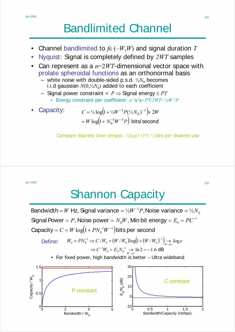
Jan 2008 181

Bandlimited Channel

• Channel bandlimited to f∈(–W,W) and signal duration T

( )( ) dbits/secon PWNW

WNPWC11

0

10

1

1log

2)(½½1log½−−

−−

+=

×+=

Compare discrete time version: ½log(1+PN–1) bits per channel use

• Capacity:

– Signal power constraint = P ⇒ Signal energy ≤ PT• Energy constraint per coefficient: n–1xTx<PT/2WT=½W–1P

– white noise with double-sided p.s.d. ½N0 becomesi.i.d gaussian N(0,½N0) added to each coefficient

• Can represent as a n=2WT-dimensional vector space with prolate spheroidal functions as an orthonormal basis

• Nyquist: Signal is completely defined by 2WT samples

Jan 2008 182

Shannon Capacity

Define:

• For fixed power, high bandwidth is better – Ultra wideband

( ) secondper bits Capacity

energy bit Min , power Noise , Power Signal

varianceNoise, varianceSignal Hz, Bandwidth

110

10

01

1log

½½

−−

−

−

+==

====

===

WPNWC

PCEWNP

NPWW

b

( ) ( )( ) eWWWWWCPNWW

log/1log// 1000

100 ∞→

−− →+=⇒=

dB 6.12ln100

1 −=→=⇒∞→

−−

WbNEWC

0 0.5 1 1.5 2-10

0

10

20

30

Bandwidth/Capacity (Hz/bps)

Eb/N

0 (

dB

)

0 2 4 60

0.5

1

1.5

Bandwidth / W0

Ca

pa

city

/ W

0

P constant

C constant

Jan 2008 183

Practical Channel Codes

Code Classification:– Very good: arbitrarily small error up to the capacity– Good: arbitrarily small error up to less than capacity– Bad: arbitrarily small error only at zero rate (or never)

Practical Good Codes:– Practical: Computation & memory ∝ nk for some k– Convolution Codes: convolve bit stream with a filter

• Concatenation, Interleaving, turbo codes (1993)– Block codes: encode a block at a time

• Hamming, BCH, Reed-Solomon, LD parity check (1995)

Coding Theorem: Nearly all codes are very good– but nearly all codes need encode/decode computation ∝ 2n

Jan 2008 184

Channel Code Performance

• Power Limited– High bandwidth– Spacecraft, Pagers– Use QPSK/4-QAM– Block/Convolution Codes

Diagram from “An overview of Communications” by John R Barry, TTC = Japanese Technology Telecommunications Council

• Value of 1 dB for space– Better range, lifetime,

weight, bit rate– $80 M (1999)

• Bandwidth Limited– Modems, DVB, Mobile

phones– 16-QAM to 256-QAM– Convolution Codes

Jan 2008 185

Lecture 15

• Parallel Gaussian Channels– Waterfilling

• Gaussian Channel with Feedback

Jan 2008 186

Parallel Gaussian Channels

• n gaussian channels (or one channel n times)– e.g. digital audio, digital TV, Broadband ADSL

• Noise is independent zi ~ N(0,Ni)

• Average Power constraint ExTx ≤ P+

x1 y1

z1

+xn yn

zn

);(max:)(

yxxx

ICPEf T

f ≤=

x

• What is the optimal f(x) ?

• R<C ⇔ R achievable– proof as before

• Information Capacity:

Jan 2008 187

Parallel Gaussian: Max Capacity

Need to find f(x):

( )∑=

−+≤n

iii NP

1

11log½(b)

Translation invariance

x,z indep; Zi indep

(a) indep bound;(b) capacity limit

Equality when: (a) yi indep ⇒ xi indep; (b) xi ~ N(0, Pi)

( )∑=

−+n

iii NP

1

11log½

);(max:)(

yxxx

ICPEf T

f ≤=

x

We need to find the Pi that maximise

)|()();( xyyyx hhI −= )|()( xzy hh −=

)()( zy hh −= ∑=

−=n

iihh

1

)()( zy

( )∑=

−≤n

iii hh

1

)()( zy(a)

Jan 2008 188

Parallel Gaussian: Optimal Powers

We need to find the Pi that maximise– subject to power constraint

( )∑=

−+n

iii NPe

1

11ln½)log(

1½ −=+⇒ λii NP

PPn

ii =∑

=1

1

11

½−

==

⎟⎠

⎞⎜⎝

⎛ +=⇒= ∑∑n

ii

n

ii NPnPP λ Also

Water Filling: put most power into least noisy channels to make equal power + noise in each channel

N1

P1

N2

P2

N3

P3

½λ–1

– use Lagrange multiplier

( ) ∑∑==

− −+=n

ii

n

iii PNPJ

11

11ln½ λ

( ) 0½ 1 =−+=∂∂ − λii

i

NPP

J

Jan 2008 189

Very Noisy Channels

• Must have Pj ≥ 0 ∀i

• If ½λ–1 < Nj then set Pj=0 and recalculate λ

N1

P1

N2

P2 N3

½λ–1

Kuhn Tucker Conditions:(not examinable)– Max f(x) subject to Ax+b=0 and

concave with for ii gfMig ,:10)( ∈≥x

Axxxx TM

iii gfJ λ−−= ∑

=1

)()()( μ

0)(,0,0)(,,0)( 000 =≥≥=+=∇ xx0bAxx iiii ggJ μμ– Solution x0, λ, μi iff

– set

Jan 2008 190

Correlated Noise

• Suppose y = x + z where E zzT = KZ and E xxT = KX

( ) nPnPEn

ii ≤⇔≤∑

=XKtr

1

2x

IQQQDQK == TTZ with

( ) ( ) ( )XT

XXT KQQKQKQ trtrtr ==

( )DDIQKQ tr1−+=−= nPLLXT where

( ) TX L QDIQK −=⇒

– Choose

– Power constraint is unchanged

• ⇒ Wi are now independent

– Now QTy = QTx + QTz = QTx + w

where E wwT = E QTzzTQ = E QTKZQ = D is diagonal

– Find noise eigenvectors:

• We want to find KX to maximize capacity subject to

power constraint:

Jan 2008 191

Power Spectrum Water Filling

• If z is from a stationary process then diag(D) power spectrum

-0.5 0 0.50

0.5

1

1.5

2

2.5

3

3.5

4

4.5

5

Frequency

Noise Spectrum

-0 .5 0 0 .50

0 .5

1

1 .5

2

F re q u e n c y

T ra n s m it S p e c tru m( )df

fN

fNLC

W

W∫− ⎟⎟⎠

⎞⎜⎜⎝

⎛ −+=

)(

0),(max1log½

( ) dffNLPW

W∫− −= 0),(max

∞→→

n

– To achieve capacity use waterfilling on noise power spectrum

L

Jan 2008 192

Gaussian Channel + Feedback

Does Feedback add capacity ?+

xi yi

zi

Coderw

( )1:1, −= iii x ywx

z

y

K

Klog½=

xi=xi(w,y1:i–1), z = y – x

z = y – x and translation invariance

zi depends only on z1:i–1

⇒ maximize I(w ; y) by maximizing h(y) ⇒ y gaussian

⇒ we can take z and x = y – z jointly gaussian

Chain rule

Chain rule, ( ) bitsZz Keh π2log½)( =

– White noise – No– Coloured noise – Not much

)|()();( ww yyy hhI −= ∑=

−−=n

iiihh

11:1 ),|()( ywyy

∑=

−−−=n

iiiiihh

11:1:11:1 ),,,|()( zxywyy

∑=

−−−=n

iiiiihh

11:1:11:1 ),,,|()( zxywzy

∑=

−−=n

iiihh

11:1 )|()( zzy

)()( zy hh −=

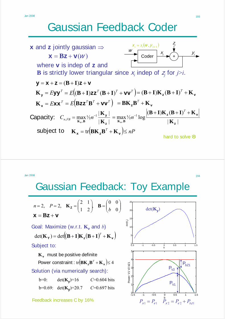
Jan 2008 193

Gaussian Feedback Coder

x and z jointly gaussian ⇒

where v is indep of z andB is strictly lower triangular since xi indep of zj for j>i.

+xi yi

zi

Coderw

( )1:1, −= iii x ywx

)(wvzx += B

Capacity:

subject to

||

)()(log½max 1

,z

vz

v K

KIBKIB

BK

+++= −

T

n

( ) nPT ≤+= vzx KBBKK trhard to solve

vzzxy ++=+= )( IBTEyyy =K ( )TTTE vvzz +++= )()( IBIB vz KIBKIB +++= T)()(

TExxx =K ( )TTTE vvzz += BB vz KBBK += T

||

||½max 1

,,

z

y

v K

KBK

−= nC FBn

Jan 2008 194

-1.5 -1 -0.5 0 0.5 1 1.50

1

2

3

4

5

b

Po

we

r: V

1 V

2 b

Z1

Gaussian Feedback: Toy Example

⎟⎟⎠

⎞⎜⎜⎝

⎛=⎟⎟

⎠

⎞⎜⎜⎝

⎛===

0

00,

21

12,2,2

bPn BKZ

-1.5 -1 -0.5 0 0.5 1 1.50

5

10

15

20

25

b

de

t(K

Y)

det(Ky)

PbZ1

PV1

PV2

vzx += B

( ) ( )( )vzY KIBKIBK +++= Tdet)det(

Goal: Maximize (w.r.t. Kv and b)

Subject to:

( ) 4tr ≤+ vz

v

KBBK

KT :constraintPower

definite positive bemust

Solution (via numerically search):

b=0: det(Ky)=16 C=0.604 bits

Feedback increases C by 16% 12211 zvxvx bPPPPP +==

b=0.69: det(Ky)=20.7 C=0.697 bits

Jan 2008 195

Max Benefit of Feedback: Lemmas

Lemma 1: Kx+z+Kx–z = 2(Kx+Kz)( )( ) ( )( )( )( ) ( )zx

zxzx

zzxx

zzzxxzxxzzzxxzxx

zxzxzxzx

KK

KK

+=+=

+−−++++=

−−+++=+ −+

222 TT

TTTTTTTT

TT

E

E

EE

Lemma 2: If F,G are +ve definite then det(F+G)≥det(F)

Conditioning reduces h()Translation invariance

f,g independent

Hence: det(2(Kx+Kz)) = det(Kx+z+Kx–z) ≥ det(Kx+z) = det(Ky)

( )( ) )()det(2log½ gf +=+ he n GFπ)|()|( gfggf hh =+≥

( )( ))det(2log½)( Fneh π== f

Consider two indep random vectors f~N(0,F), g~N(0,G)

Jan 2008 196

Maximum Benefit of Feedback

Having feedback adds at most ½ bit per transmission

( )missionbits/trans n

nPCn +=

++= −

≤½

)det(

detlog½max½ 1

)tr(z

zx

x K

KKK

det(kA)=kndet(A)

Lemmas 1 & 2:

det(2(Kx+Kz)) ≥ det(Ky)

no constraint on B ⇒ ≤

+xi yi

zi

Coderw

)det(

)det(log½max 1

)tr(,

z

y

x K

KK

−

≤≤ nC

nPFBn

( )( ))det(

2detlog½max 1

)tr(z

zx

x K

KKK

+≤ −

≤n

nP

( ))det(

det2log½max 1

)tr(z

zx

x K

KKK

+= −

≤

n

nPn

Ky = Kx+Kz if no feedback

Jan 2008 197

Lecture 16

• Lossy Coding• Rate Distortion

– Bernoulli Scurce– Gaussian Source

• Channel/Source Coding Duality

Jan 2008 198

Lossy Coding

Distortion function:– examples: (i) (ii)

x1:n Encoderf( )

f(x1:n)∈1:2nRDecoder

g( )

x1:n^

0)ˆ,( ≥xxd2)ˆ()ˆ,( xxxxdS −=

⎩⎨⎧

≠=

=xx

xxxxdH ˆ1

ˆ0)ˆ,(

∑=

−Δ=

n

iii xxdnd

1

1 )ˆ,()ˆ,( xx

( ) ( )))((,ˆ, xxxxx

fgdEdED n == ∈X

DfgdE nnn

n ≤∈∞→

)))((,(lim xxx X

Rate distortion pair (R,D) is achievable for source X if∃ a sequence fn() and gn() such that

Distortion of Code fn(),gn():

– sequences:

Jan 2008 199

Rate Distortion Function

Rate Distortion function for {xi} where p(x) is known is

DdE

p

pIDR

≤

=

)ˆ,(

)(

)ˆ,()ˆ;(min)(

ˆ, xxx

xxxx

xx(b)

correct is (a):that such allover

achievable is that such (R,D)RDR inf)( =

We will prove this next lecture

If D=0 then we have R(D)=I(x ; x)=H(x)

– this expression is the Information Rate Distortion function for X

Theorem:

Jan 2008 200

R(D) bound for Bernoulli Source

Bernoulli: X = [0,1], pX = [1–p , p] assume p ≤ ½– Hamming Distance: xxxxd ˆ)ˆ,( ⊕=

then DxxdE ≤)ˆ,(

monotonic as

for so and

)()()ˆ(

½)ˆ(

pHDHH

DDp

≤⊕

≤≤⊕

xxxx

Conditioning reduces entropy

⊕ is one-to-one

Hence R(D) ≥ H(p) – H(D)

0 0.1 0.2 0.3 0.4 0.50

0.2

0.4

0.6

0.8

1

D

R(D

), p

=0

.2,0

.5

p=0.2

p=0.5

– For D < p ≤ ½, if

– If D≥p, R(D)=0 since we can set g( )≡0

)ˆ|()()ˆ;( xxxxx HHI −=

)ˆ|ˆ()( xxx ⊕−= HpH

)ˆ()( xx ⊕−≥ HpH

)()( DHpH −≥

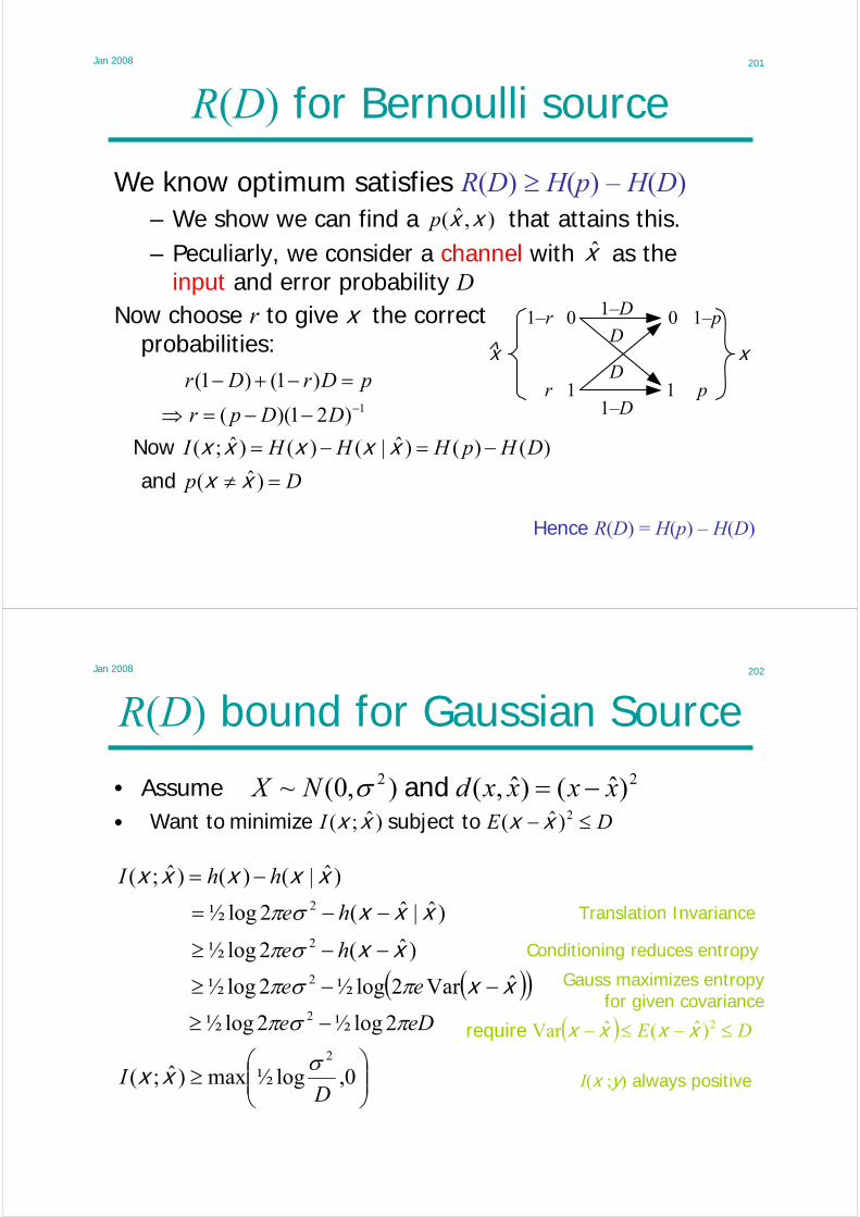
Jan 2008 201

R(D) for Bernoulli source

We know optimum satisfies R(D) ≥ H(p) – H(D)– We show we can find a that attains this.),ˆ( xxp

x

D

0

1

0

1

xD

1–D

1–D

x

1–p

p

1–r

r

Now choose r to give x the correct probabilities:

Hence R(D) = H(p) – H(D)

– Peculiarly, we consider a channel with as the input and error probability D

Dp

DHpHHHI

=≠

−=−=

)ˆ(

)()()ˆ|()()ˆ;(

xxxxxxx

and

Now

1)21)((

)1()1(−−−=⇒

=−+−

DDpr

pDrDr

Jan 2008 202

R(D) bound for Gaussian Source

• Assume 22 )ˆ()ˆ,(),0(~ xxxxdNX −= and σ

Translation Invariance

Conditioning reduces entropy

Gauss maximizes entropyfor given covariance

( ) DE ≤−≤− 2)ˆ(ˆVar xxxx require

DEI ≤− 2)ˆ()ˆ;( xxxx tosubject minimize toWant

I(x ;y) always positive

•

)ˆ|()()ˆ;( xxxxx hhI −=

)ˆ|ˆ(2log½ 2 xxx −−= heσπ

)ˆ(2log½ 2 xx −−≥ heσπ

( )( )xx ˆVar2log½2log½ 2 −−≥ ee πσπ

eDe πσπ 2log½2log½ 2 −≥

⎟⎟⎠

⎞⎜⎜⎝

⎛≥ 0,log½max)ˆ;(

2

DI

σxx

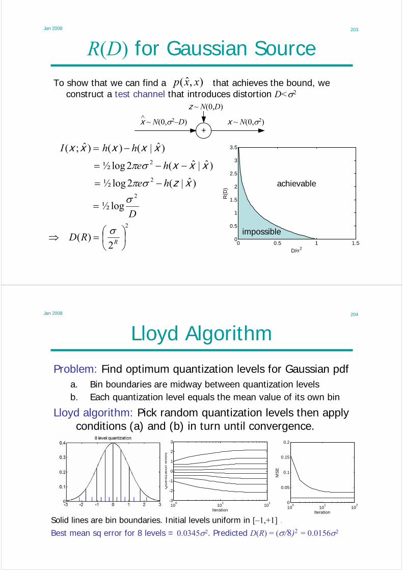
Jan 2008 203

R(D) for Gaussian SourceTo show that we can find a that achieves the bound, we

construct a test channel that introduces distortion D<σ2

+

z ~ N(0,D)

x ~ N(0,σ2)x ~ N(0,σ2–D)^

0 0.5 1 1.50

0.5

1

1.5

2

2.5

3

3.5

D/σ2

R(D

)

achievable

impossible

),ˆ( xxp

)ˆ|()()ˆ;( xxxxx hhI −=

)ˆ|ˆ(2log½ 2 xxx −−= heσπ

)ˆ|(2log½ 2 xzhe −= σπ

D

2

log½σ

=

2

2)( ⎟

⎠⎞

⎜⎝⎛=⇒

RRD

σ

Jan 2008 204

Lloyd Algorithm

Problem: Find optimum quantization levels for Gaussian pdf

100

101

102

-3

-2

-1

0

1

2

3

Iteration

Qu

an

tiza

tion

leve

ls

100

101

102

0

0.05

0.1

0.15

0.2

Iteration

MS

E

Solid lines are bin boundaries. Initial levels uniform in [–1,+1] .

Lloyd algorithm: Pick random quantization levels then apply conditions (a) and (b) in turn until convergence.

b. Each quantization level equals the mean value of its own bina. Bin boundaries are midway between quantization levels

Best mean sq error for 8 levels = 0.0345σ2. Predicted D(R) = (σ/8)2 = 0.0156σ2

Jan 2008 205

Vector Quantization

To get D(R), you have to quantize many values together– True even if the values are independent

0 0.5 1 1.5 2 2.50

0.5

1

1.5

2

2.5D = 0.035

Two gaussian variables: one quadrant only shown– Independent quantization puts dense levels in low prob areas– Vector quantization is better (even more so if correlated)

0 0.5 1 1.5 2 2.50

0.5

1

1.5

2

2.5D = 0.028

Jan 2008 206

Multiple Gaussian Variables

• Assume x1:n are independent gaussian sources with different variances. How should we apportion the available total distortion between the sources?

( ) ( ) DndN Tii ≤−−= − xxxxxx ˆˆ)ˆ,(),0(~ 12 and σx

Mut Info Independence Boundfor independent xi

R(D) for individual Gaussian

We must find the Di that minimize ∑=

⎟⎟⎠

⎞⎜⎜⎝

⎛n

i i

i

D1

2

0,log½maxσ

• Assume

∑=

≥n

iiinn II

1:1:1 )ˆ;()ˆ;( xxxx

∑∑==

⎟⎟⎠

⎞⎜⎜⎝

⎛=≥

n

i i

in

ii D

DR1

2

1

0,log½max)(σ

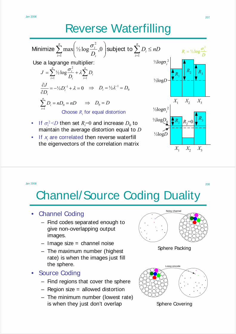
Jan 2008 207

Reverse Waterfilling

Use a lagrange multiplier:

nDDD

n

ii

n

i i

i ≤⎟⎟⎠

⎞⎜⎜⎝

⎛∑∑== 11

2

0,log½max tosubject Minimizeσ

½logσi2

½logD

R3R2R1

X1 X2 X3

½logσi2

½logD0R3R2=0R1

X3

½logD

X2X1

• If σi2 <D then set Ri=0 and increase D0 to

maintain the average distortion equal to D

Choose Ri for equal distortion

∑∑==

+=n

ii

n

i i

i DD

J 11

2

log½ λσ

0½ 1 =+−=∂∂ − λi

i

DD

J0

1½ DDi ==⇒ −λ

nDnDDn

ii ==∑

=0

1

DD =⇒ 0

• If xi are correlated then reverse waterfillthe eigenvectors of the correlation matrix

DR i

i

2

log½σ

=

Jan 2008 208

Channel/Source Coding DualityNoisy channel

• Channel Coding– Find codes separated enough to

give non-overlapping output images.

– Image size = channel noise– The maximum number (highest

rate) is when the images just fill the sphere. Lossy encode

Sphere Packing

Sphere Covering

• Source Coding– Find regions that cover the sphere– Region size = allowed distortion– The minimum number (lowest rate)

is when they just don’t overlap

Jan 2008 209

Channel Decoder as Source Coder

• For , we can find a channel encoder/decoder so that

+

z1:n ~ N(0,D)

x1:n ~ N(0,σ2)Encoder Decoder

w∈2nR w∈2nR^y1:n ~ N(0,σ2–D)

( )( )121log½ −−+=≅ DDCR σDEp ii =−<≠ 2)()ˆ( yxww and ε

( ) DEEpp iiii =−≅−<≠<≠ 22 )()ˆ()ˆ(ˆ yxxxyxww and also , εε

We have encoded x at rate R=½log(σ2D–1) with distortion D

+

Z1:n ~ N(0,D)

X1:n ~ N(0,σ2)Encoder Decoder

W Y1:nEncoder

X1:n^

W∈2nR^

• Reverse the roles of encoder and decoder. Since

Jan 2008 210

High Dimensional Space

In n dimensions– “Vol” of unit hypercube: 1– “Vol” of unit-diameter hypersphere:

– “Area” of unit-diameter hypersphere:

– >63% of Vn is in shell

( )⎩⎨⎧ −

=−

−

even odd

nn

nnnV

nn

n

n)!/(½2

!/!½½½

½½

ππ

( ) nr

nnn nVVr

dr

dA 22

½

===

3.7e–681.9e–70100

5e–22.5e–310

2.470.314

3.140.523

3.140.792

211

AnVnn

RrRn ≤≤− − )1( 1

( ) 3679.01 =→ −<

∞→e

n

n1-n-1 :Proof Most of n-dimensional space is in the corners

Jan 2008 211

Lecture 17

• Rate Distortion Theorem

Jan 2008 212

Review

Rate Distortion function for x whose px(x) is known is

x1:n Encoderfn( )


gn( )

x1:n^

DdEgfRDR nn

nn ≤∃= ∈∞→)ˆ,(lim,inf)( xx

x X with that such

DdExxpIDR ≤= )ˆ,()|ˆ()ˆ;(min)( ˆ, xxxx xxthat such allover

0 0.5 1 1.50

0.5

1

1.5

2

2.5

3

3.5

D/σ2

R(D

) achievable

impossibleR(D) curve depends on your choice of d(,)

We will prove this theorem for discrete Xand bounded d(x,y)≤dmax

Rate Distortion Theorem:

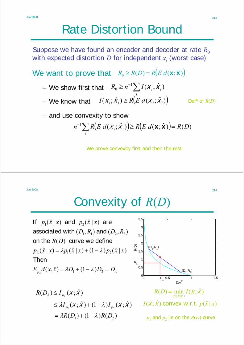
Jan 2008 213

Rate Distortion Bound

We want to prove that

∑−≥i

iiInR )ˆ;(10 xx

( ))ˆ;()ˆ;( iiii dERI xxxx ≥

( ) ( ) )()ˆ;()ˆ;(1 DRdERdERni

ii =≥∑− xxxx

We prove convexity first and then the rest

Defn of R(D)

Suppose we have found an encoder and decoder at rate R0

with expected distortion D for independent xi (worst case)

( ))ˆ;()(0 xxdERDRR =≥

– and use convexity to show

– We know that

– We show first that

Jan 2008 214

Convexity of R(D)

λ

λ

λλ

λλ

λDDDxxdE

xxpxxpxxp

DR

RDRD

xxpxxp

p =−+=

−+=

21

21

2211

21

)1()ˆ,(

)|ˆ()1()|ˆ()|ˆ(

)(

),(),(

)|ˆ()|ˆ(

Then

define we curve the on

and with associated

are and If

0 0.5 1 1.50

0.5

1

1.5

2

2.5

3

3.5

D/σ2

R(D

)

Rλ

Dλ

(D1,R

1)

(D2,R

2)

)|ˆ()ˆ;( xxpI w.r.t.convex xx

p1 and p2 lie on the R(D) curve

)ˆ;(min)()|ˆ(

xxxx

IDRp

=)ˆ;()( xxλλ pIDR ≤

)ˆ;()1()ˆ;(21

xxxx pp II λλ −+≤

)()1()( 21 DRDR λλ −+=

Jan 2008 215

Proof that R ≥ R(D)

Definition of I(;)

bound; Uniform

xi indep: Mut InfIndependence Bound

definition of R

convexity

original assumption that E(d) ≤ Dand R(D) monotonically decreasing

)ˆ( :10 nHnR x≥ )|ˆ()ˆ( :1:1:1 nnn HH xxx −=

);ˆ( :1:1 nnI xx=

∑=

≥n

iiiI

1

)ˆ;( xx

( ) ( )∑∑=

−

=

=≥n

iii

n

iii dERnndER

1

1

1

)ˆ;()ˆ;( xxxx

⎟⎠

⎞⎜⎝

⎛≥ ∑

=

−n

iiidEnnR

1

1 )ˆ;( xx ( ))ˆ;( :1:1 nndEnR xx=

)(DnR≥

0)|ˆ( =xxH

defn of vector d( )

Jan 2008 216

Rate Distortion Achievability

We want to show that for any D, we can find an encoder and decoder that compresses x1:n to nR(D) bits.

• pX is given• Assume we know the that gives

x1:n Encoderfn( )


gn( )

x1:n^

)|ˆ( xxp )()ˆ;( DRI =xx

xx ˆ~ˆ pi

First define the typical set we will use, then prove two preliminary results.

• Encoder: Use joint typicality to design

– We show that there is almost always a suitable codeword

• Random Decoder: Choose 2nR random– There must be at least one code that is as good as the average

Jan 2008 217

Distortion Typical SetDistortion Typical:

{

}εε

ε

εε

<−

<−−

<−−

<−−×∈=

−

−

−

)ˆ,()ˆ,(

)ˆ,()ˆ,(log

,)ˆ()ˆ(log

,)()(log:ˆˆ,

1

1

1)(,

xx

xx

x

x

dEd

Hpn

Hpn

HpnJ nnnd

xx

xx

x

xxx XX

( ) εε nnHpJ nd ±−=⇒∈ )ˆ,(ˆ,logˆ, )(

, xxxxxx

( ) εε ε NnJp nd >−>∈ for1ˆ, )(

,xx

( ) )x~p(x,ii ˆˆˆ, i.i.d. drawn XX×∈xx

new condition

i.i.d. are numbers; large of law weak )ˆ,( iid xx

2. Total Prob:

1. Indiv p.d.:

Properties:

Jan 2008 218

Conditional Probability Bound

Lemma: ( ) ( ) ( )εε

3)ˆ;()(, 2|ˆˆˆ, +−≥⇒∈ xxInn

d ppJ xxxxx

bounds from defn of J

defn of I

take max of top and min of bottom

( ) ( )( )x

xxxx

p

pp

,ˆ|ˆ =

( ) ( )( ) ( )xx

xxx

pp

pp

ˆ,ˆ

ˆ=

( )( )

( ) ( )εε

ε

+−+−

−−

≤)ˆ()(

)ˆ,(

22

2ˆ

xx

xx

HnHn

Hn

p x

( ) ( )ε3)ˆ;(2ˆ += xxInp x

Proof:

Jan 2008 219

Curious but necessary InequalityLemma: vmm euuvmvu −+−≤−⇒>∈ 1)1(0],1,0[,

vmmvm ee −− +−≤−⇒≥ 01)01(0

convexity for u,v ∈ [0,1]

for u,v ∈ [0,1]

0<u<1:

u=1:Proof: u=0:

vv evfvevf −− −=′⇒+−= 1)(1)( Define

]1,0[0)(00)(0)0( ∈≥⇒>>′= vvfvvff for for and

( ) vmmv evevv −− ≤−⇒≤−≤∈ 110],1,0[for Hence

mv uvug )1()( −= Define

convex )(0)1()1()( 22 uguvvmmxg vn

v ⇒≥−−=′′⇒ −

)1()0()1()()1( vvvm ugguuguv +−≤=−

vmvmm euueuvuu −− +−≤+−≤−+−= 11)1(1)1(

Jan 2008 220

Achievability of R(D): preliminaries

•

x1:n Encoderfn( )


gn( )

x1:n^

})|ˆ()()ˆ({0

)ˆ,();()ˆ;()|ˆ(

ˆ ∑==>

≤=

x

xxpxpxp

DxxdEDRIxxpD

x

xx

p define and Choose

that such a find and Choose

δ

nwn

nR wgw x~ˆ)(2:1 px i.i.d. drawn choose eachFor =∈

w J, wf ndwn such no if else that such 1)ˆ(min)( )(

,ε∈= xxx

)ˆ,(, xxx dED g=

δ+= DD– for large n we show so there must be one good code

– over all input vectors x and all random decode functions, g

• Expected Distortion:

• Encoder:

• Decoder:

Jan 2008 221

Expected Distortion

We can divide the input vectors x into two categories:

DdE

DdJ, w wn

dw

≤

+<∈∃

)ˆ,(

)ˆ,()ˆ( )(,

xx

xxxx

since

then that such if εε

We need to show that the expected value of Pe is small

b) if no such w exists we must have since we are assuming that d(,) is bounded. Suposethe probability of this situation is Pe.

a)

)ˆ,(, xxx dED g= Hence

max))(1( dPDP ee ++−≤ ε

maxdPD e++≤ ε

max)ˆ,( dd w <xx

Jan 2008 222

Error ProbabilityDefine the set of valid inputs for code g

0)ˆ,(1)ˆ,( )(, else if Define n

dJK ε∈= xxxx

∑ ∑∑ ∑∉∉

==x xx

xx)(:)(

)()()()(gVgg gV

e gpppgpP

{ })(,))(,(:)( n

dJwgwgV ε∈∃= xx with

∑−x

xxxxxˆ

)ˆ,()ˆ(1ˆ Kp is matchnot does random athat ProbnR

Kp2

ˆ

)ˆ,()ˆ(1 ⎟⎠

⎞⎜⎝

⎛−∑

x

xxx is matchnot does code entire anthat Prob

∑ ∑ ⎟⎠

⎞⎜⎝

⎛−=

x x

xxxx

nR

KppPe

2

ˆ

)ˆ,()ˆ(1)( Hence

We have

Jan 2008 223

Achievability for average codeSince ( ) ( ) ( )ε

ε3)ˆ;()(

, 2|ˆˆˆ, +−≥⇒∈ xxInnd ppJ xxxxx

vmm euuv −+−≤− 1)1( Using

( )∑ ∑ ⎟⎠

⎞⎜⎝

⎛−≤ +−

x x

xxxxx

nR

InKpp2

ˆ

3)ˆ;(2)ˆ,()|ˆ(1)( εxx

∑ ∑ ⎟⎠

⎞⎜⎝

⎛−=

x x

xxxx

nR

KppPe

2

ˆ

)ˆ,()ˆ(1)(

( )( )∑ ∑ ⎟⎠

⎞⎜⎝

⎛−+−≤ +−

x x

xxxxxˆ

3)ˆ;( 22exp)ˆ,()|ˆ(1)( nRInKpp εxx

nRnnI mvKpu 2;2;)ˆ,()|ˆ( 3)ˆ;(

ˆ

=== −−∑ εxx

x

xxxx with

requiredas :Note 1,0 ≤≤ vu

Jan 2008 224

Achievability for average code

δδ +≤=>∀ DdED g made be can Hence )ˆ,(,0 , xxx

( )( )∑ ∑ ⎟⎠

⎞⎜⎝

⎛−+−≤ +−

x x

xxxxxˆ

3)ˆ;( 22exp)ˆ,()|ˆ(1)( nRXXIne KppP ε

( )( )( ) ∑−−+= +−

xx

xxxxxˆ,

3)ˆ;( )ˆ,()|ˆ()(22exp1 KppnRXXIn ε

( )( )ε3)ˆ;(

ˆ,

2exp)ˆ,()ˆ,(1 −−−+−= ∑ XXIRnKpxx

xxxx

take out terms not involving x

{ } ( )( )εε

3)ˆ;()(, 2exp)ˆ,( −−−+∉= XXIRnn

dJP xx

ε3)ˆ,(0 +>∞→→ xxInRn provided as terms both

0⎯⎯ →⎯ ∞→n

Jan 2008 225

Achievability

Hence (R,D) is achievable for any R>R(D)

δ

δδ

+≤

+≤=>∀

DdEg

DdED g

with oneleast at bemust there

made be can Since

)ˆ,(

)ˆ,(,0 ,

xx

xx

x

x

DEnX

n≤

∞→)ˆ,(lim

:1xx isthat

x1:n Encoderfn( )


gn( )

x1:n^

In fact a stronger result is true:

1))ˆ,((,),(,0∞→

→+≤∃>>∀n

nn DdpgfDRRD δδ xx with and

Jan 2008 226

Lecture 18

• Revision Lecture

Jan 2008 227

Summary (1)• Entropy:

– Bounds:– Conditioning reduces entropy:– Chain Rule:

• Relative Entropy:

))((log)(log)()( 22 xpExpxpH Xx

−=−×= ∑∈X

x

Xlog)(0 ≤≤ xH

)()|( yxy HH ≤

∑

∑∑

=

==−

≤

≤=

n

iiinn

n

ii

n

iiin

HH

HHH

1:1:1

111:1:1

)|()|(

)()|()(

yxyx

xxxx

( ) ( ) 0)(/)(log|| ≥= xx qpED pqp

Jan 2008 228

Summary (2)• Mutual Information:

– Positive and Symmetrical:– x, y indep ⇔– Chain Rule:

0);()()(),( =⇔+= yxxyyx IHHH

( )yxyxyxyxxyyxy

ppp ||),()()(

)|()();(

,DHHH

HHI

=−+=−=

0);();( ≥= xyyx II

∑=

−=n

iiin II

11:1:1 )|;();( xyxyx

∑

∑

=−

=

≤⇒=

≥⇒

n

iiinniiini

n

iiinni

IIpp

II

1:1:11:1:1

1:1:1

);();()|();|(

);();(tindependen

yxyxxyyxy

yxyxx

H(x |y) H(y |x)

H(x ,y)

H(x) H(y)

I(x ;y)

Jan 2008 229

Summary (3)

• Convexity: f’’ (x) ≥ 0 ⇒ f(x) convex ⇒ Ef(x) ≥ f(Ex)– H(p) concave in p– I(x ; y) concave in px for fixed py|x

– I(x ; y) convex in py|x for fixed px

• Markov:⇒ I(x ; y) ≥ I(x ; z) and I(x ; y) ≥ I(x; y | z)

• Fano:

• Entropy Rate:– Stationary process

– Markov Process:

– Hidden Markov:

0)|;()|(),|( =⇔=⇔→→ yzxzyx Iyzpyxzp

( ) ( )1||log

1)|(ˆˆ−−

≥≠⇒→→Xyxxxxyx H

p

)(lim)( :11

nn

HnH x−

∞→=X

)|()( 1:1 −≤ nnHH xxX

)|(lim)( 1−∞→= nn

nHH xxX

)|()(),|( 1:111:1 −− ≤≤ nnnn HHH yyxyy Y ∞→= n as

∞→= n as

= if stationary

Jan 2008 230

Summary (4)

• Kraft: Uniquely Decodable ⇒ ⇒ ∃ prefix code

• Average Length: Uniquely Decodable ⇒ LC = E l(x) ≥ HD(x)

• Shannon-Fano: Top-down 50% splits. LSF ≤ HD(x)+1

• Shannon:• Huffman: Bottom-up design. Optimal.

– Designing with wrong probabilities, q ⇒ penalty of D(p||q)

– Long blocks disperse the 1-bit overhead

• Arithmetic Coding:– Long blocks reduce 2-bit overhead– Efficient algorithm without calculating all possible probabilities– Can have adaptive probabilities

1||

1

≤∑=

−X

i

liD

⎡ ⎤ 1)()(log +≤−= xDSDx HLxpl

1)( +≤ xDH HL

∑<

=NN

i xx

Ni

N xpxC )()(

Jan 2008 231

Summary (5)

• Typical Set– Individual Prob– Total Prob– Size– No other high probability set can be much smaller

• Asymptotic Equipartition Principle– Almost all event sequences are equally surprising



22)1( ))(()())(( εε

ε ε

ε +>


Hn T

Jan 2008 232

Summary (6)

• DMC Channel Capacity:• Coding Theorem

– Can achieve capacity: random codewords, joint typical decoding– Cannot beat capacity: Fano

• Feedback doesn’t increase capacity but simplifies coder• Joint Source-Channel Coding doesn’t increase capacity

);(max yxx

ICp

=

Jan 2008 233

Summary (7)

• Differential Entropy:– Not necessarily positive– h(x+a) = h(x), h(ax) = h(x) + log|a|, h(x|y) ≤ h(x)

– I(x; y) = h(x) + h(y) – h(x, y) ≥ 0, D(f||g)=E log(f/g) ≥ 0

• Bounds:– Finite range: Uniform distribution has max: h(x) = log(b–a)

– Fixed Covariance: Gaussian has max: h(x) = ½log((2πe)n|K|)

• Gaussian Channel– Discrete Time: C=½log(1+PN–1)

– Bandlimited: C=W log(1+PN0–1W–1)

• For constant C: – Feedback: Adds at most ½ bit for coloured noise

)(log)( xx xfEh −=

( ) ( )( ) dB 6.12ln12/1/1

011

0 −=→−==∞→

−−− −

W

CWb CWNPCNE

Jan 2008 234

Summary (8)

• Parallel Gaussian Channels: Total power constraint– White noise: Waterfilling:– Correlated noise: Waterfill on noise eigenvectors

• Rate Distortion:

– Bernoulli Source with Hamming d: R(D) = max(H(px)–H(D),0)

– Gaussian Source with mean square d: R(D) = max(½log(σ2 D–1),0)

– Can encode at rate R: random decoder, joint typical encoder

– Can’t encode below rate R: independence bound

• Lloyd Algorithm: iterative optimal vector quantization

∑ = PPi

( )0,max 0 ii NPP −=

)ˆ;(min)()ˆ,(..|ˆ

xxxxxx

IDRDEdts ≤

=p

information theory - ee.ic.ac.uk · pdf fileinformation theory mike brookes e4.40, ise4.51,...

Documents