information theory and statistics -

Chapter 12

Information Theory and Statistics

We now explore the relationship between information theory and statistics. We begin by describing the method of types, which is a powerful technique in large deviation theory. We use the method of types to calculate the probability of rare events and to show the existence of universal source codes. We also consider the problem of testing hypotheses and derive the best possible error exponents for such tests (Stein’s lemma). Finally, we treat the estimation of the parameters of a distribution and describe the role of Fisher information.

12.1 THE METHOD OF TYPES

The AEP for discrete random variables (Chapter 3) focuses our atten- tion on a small subset of typical sequences. The method of types is an even more powerful procedure in which we consider the sequences that have the same empirical distribution. With this restriction, we can derive strong bounds on the number of sequences of a particular empirical distribution and the probability of each sequence in this set. It is then possible to derive strong error bounds for the channel coding theorem and prove a variety of rate-distortion results. The method of types was fully developed by Csiszar and Korner [83], who obtained most of their results from this point of view.

Let X1,X,, . . . ,X, be a sequence of n symbols from an alphabet 2 = {a,, fJ2, * * * , a,*,). We will use the notation xn and x interchange- ably to denote a sequence ;xl, x2, . . . , x, .

Definition: The type P, (or empirical probability distribution) of a sequence x,, x,, . . . , x, is the relative proportion of occurrences of each

279

Elements of Information TheoryThomas M. Cover, Joy A. Thomas

Copyright 1991 John Wiley & Sons, Inc.Print ISBN 0-471-06259-6 Online ISBN 0-471-20061-1

280 ZNFORMATZON THEORY AND STATZSTZCS

symbol of %‘, i.e., P&z) = N(alx)ln for all a E %‘, where N(aIx) is the number of times the symbol a occurs in the sequence x E %“.

The type of a sequence x is denoted as P,. It is a probability mass function on Z. (Note that in this chapter, we will use capital letters to denote types and distributions. We will also loosely use the word “distribution” to mean a probability mass function.)

Definition: Let 9,, denote the set of types with denominator n.

For example, if 8? = (0, l}, then the set of possible types with denominator n is

~~={(P(o),PUk(;, ;),(;,g ,..., (I, !)}. (12.1)

DefZnition: If P E P,,, then the set of sequences of length n and type P is called the type class of P, denoted T(P), i.e.,

T(P)= {XEr:P,=P}. (12.2)

The type class is sometimes called the composition class of P.

EmmpZe 12.1.1: Let %‘= {1,2,3}, a ternary alphabet. Let x = 11321. Then the type P, is

P,(l)= 5, P,(2)= 5, P,(3)= 5. (12.3)

The type class of P, is the set of all sequences of length 5 with three l’s, one 2 and one 3. There are 20 such sequences, and

T(P,) = {11123,11132,11213,. . . ,321ll) . (12.4)

The number of elements in T(P) is

IzIP,I=(,; 1)=&=20. 9 9 . . . (12.5)

The essential power of the method of types arises from the following theorem, which shows that the number of types is at most polynomial in n.

Theorem 12.1.1:

lgnl 22 (n + l)l&( . (12.6)

12.1 THE METHOD OF TYPES 281

Proof: There are 1 Z 1 components in the vector that specifies Px. The numerator in each component can take on only n + 1 values. So there are at most (n + l)la”’ choices for the type vector. Of course, these choices are not independent (for example, the last choice is fixed by the others). But this is a sufficiently good upper bound for our needs. Cl

The crucial point here is that there are only a polynomial number of types of length n. Since the number of sequences is exponential in n, it follows that at least one type has exponentially many sequences in its type class. In fact, the largest type class has essentially the same number of elements as the entire set of sequences, to first order in the exponent.

Now, we will assume that the sequence X,, X,, . . . , X, is drawn i.i.d. according to a distribution Q(x). AI1 sequences with the same type will have the same probability, as shown in the following theorem. Let Q”(x”) = II;=, Q&) denote the product distribution associated with Q.

Theorem 12.1.2: If X1,X,, . . . ,X, are drawn Cd. according to Q(x), then the probability of x depends only on its type and is given by

Proof:

Q”(x) = 2- nW(P,&+D(P,"Q)) .

Q”(x) = ii Q(xi) i=l

= fl Q(a)N(uIx) aE&”

= n Q(a)npJa) aE%

= l-I 2 nP,(u) log Q(a)

UEEe”

= n 2 n(P.,&z) log Q(a)-P,(a) log P&)+P,b) log P,(a))

aE%

nC = 2

aE* (-P,(a) log ~+PJaI logP,W

= p-NP,llQ)-H(P,H . q

Corollary: If x is in the type class of Q, then

Qn(x) = 24(Q) .

(12.7)

(12.8)

(12.9)

(12.10)

(12.11)

(12.12)

(12.13)

(12.14)

(12.15)

282 1NFORMATlON THEORY AND STATISTICS

Proof: If x E T(Q), then Px = Q, which can be substituted into (12.14). q

Example 12.1.2: The probability that a fair die produces a particular sequence of length n with precisely n/6 occurrences of each face (n is a multiple of 6) is 2-nHcaP 8’. . . ’ Q’ = 6-“. This is obvious. However, if the die has a probability mass function ( i, $, i, &, &, 0), the probability of observing a particular sequence with precisely these frequencies is precisely 2 --nH(i, g, Q, i&P $270) f or n a multiple of 12. This is more interesting.

We now give an estimate of the size of a type class Z’(P).

Theorem 12.1.3 (Size of a type class Z’(P)): For any type P E gn,

1 (n + l)‘Z’ 2

nN(P) ( IT(P)I 5 y-) . (12.16)

Proof: The exact size of Z’(P) is easy to calculate. It is a simple combinatorial problem-the number of ways of arranging nP(a, ), nP(a,), . . . , nP(a,,,) objects in a sequence, which is

IT(P)I = ( n nP(a, 1, nP(a,), . . . , nP(algl) > ’

(12.17)

This value is hard to manipulate, so we derive simple exponential bounds on its value.

We suggest two alternative proofs for the exponential bounds. The first proof uses Stirling% formula [ 1101 to bound the factorial

function, and after some algebra, we can obtain the bounds of the theorem.

We give an alternative proof. We first prove the upper bound. Since a type class must have probability I 1, we have

11 P”(T(P)) (12.18)

= c P”(x) xE!r(P)

= x&J) 2-

nH(P 1

= IT(P))2-“H’P) ,

(12.19)

(12.20)

(12.21)

using Theorem 12.1.2. Thus

1 T(P)1 5 2nH(P) , (12.22)

12.1 THE METHOD OF 7YPES 283

Now for the lower bound. We first prove that the type class T(P) has the highest probability among all type classes under the probability distribution P, i.e.,

JWYPN 1 P”u@)), for all P E 9n . (12.23)

We lower bound the ratio of probabilities,

P”(T(PN _ JT(P)p,,, PwP(a)

P”(m) - 1 T@)ll-l,,, P(czypca) (12.24)

( nPbl), nP$?, . . . , nP(qq) ) fla,, P(cFa) =

( n

n&al), n&a2), . . . , nP(algI) >fl

(12 25)

uE* P(a)npca) *

= fl (da))! p(a)n(P(a)-B(a))

aEg WbN . (12.26)

Now using the simple bound (easy to prove by separately considering the cases m 2 n and m < n)

(12.27)

we obtain

~“UYP))

P”(m)

L n (np(u))n~(a)-nP(a)p(a)n(P(u)-~(a)) (12.28) aE2f

= l-I n n@(a)-P(a))

aEl

= nn(caEZ P(a)-C aEIP P(a))

(12.29)

=n &l-l) (12.31) .

=l. (12.32)

Hence P”(T(P)) 2 P”(@)). The lower bound now follows easily from this result, since

l= c P”U’(QN QEB,

(12.33)

(12.34)

(12.35)

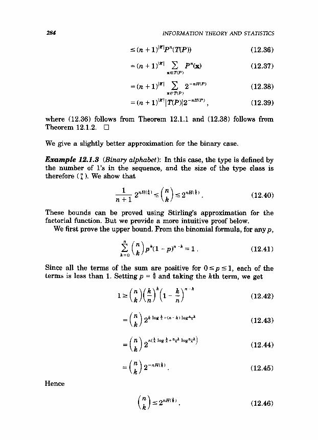
284 INFORMATZON THEORY AND STATZSTZCS

< (n + l)‘x’P”(T(P)) - (12.36)

= (n + l)‘%’ c P”(x) (12.37) XET(P)

= (n + r>l"l 2 243(P) (12.38) xET(P)

=(n + lfa'lT(P)12-nH'P' ? (12.39)

where (12.36) follows from Theorem 12.1.1 and (12.38) follows from Theorem 12.1.2. Cl

We give a slightly better approximation for the binary case.

Example 12.1.3 (Binary alphabet): In this case, the type is defined by the number of l’s in the sequence, and the size of the type class is therefore ( g ). We show that

1 -2 rzH(h< n

( > nH(!i)

n-II -k12 . (12.40)

These bounds can be proved using Stirling’s approximation for the factorial function. But we provide a more intuitive proof below.

We first prove the upper bound. From the binomial formula, for any p,

p&(1 -p)n-k = 1 . (12.41)

Since all the terms of the sum are positive for 0 I p I 1, each of the terms is less than 1. Setting p = $ and taking the Filth term, we get

k log h+(n-k) log%?

( > i2

n(h log ff+* log+ = >

= ( > nZ!Z(!i) ;2- .

(12.42)

(12.43)

(12.44)

(12.45)

nH(i) 52 . (12.46)

12.1 THE METHOD OF TYPES 285

For the lower bound, let S be a random variable with a binomial distribution with parameters n and p. The most likely value of S is S = ( np ) . This can be easily verified from the fact that

P(S=i+l)-n-i p P(S = i) i+l l-p

(12.47)

and considering the cases when i < np and when i > np. Then, since there are n + 1 terms in the binomial sum,

1= i (;)p*(l -p)n-k r(n + l)m*ax( ;)pkU -pTk k=O

(12.48)

=(n+l)( (&) > p’“P’(l -p)“-‘“P’ .

(12.49)

Now let p = $. Then we have

l~~n+l)(~)(t)k(l-%)“-k, (12.50)

which by the arguments in (12.45) is equivalent to

1 -2s n-+1

(12.51)

or

(12.52)

Combining the two results, we see that

(12.53)

Theorem 12.1.4 (Probdbility of type c2ass): For any P E gn and any distribution Q, the probability of the type class T(P) under Q” is 2-nD’p”Q) to first order in the exponent. More precisely,

cyD(PllQ) I Q”(T(p)) I 2-nDU-‘llQ) . (12.54)

Proof: We have

&VW) = c Q”(x) XET(P)

(12.55)

286 UVFORMATION THEORY AND STATZSTlCS

= IT(P)12- n(D(P(lQ)+H(PN 2

(12.56)

(12.57)

by Theorem 12.1.2. Using the bounds on IT(P)) derived in Theorem 12.1.3, we have

1 (n + 1)'"'

2-no(pllQ)IQn(~(p))~2-no(pltQ). q (12.58)

We can summarize the basic theorems concerning types in four equations:

lLPnl I (n + 1)‘“’ , (12.59)

Q"(x)= 2- n(D(P,llQ)+H(P,N 7

1 T(P)1 A 2nH(P) ,

Qn(T(p))~2-'11Q) . (12.62)

These equations state that there are only a polynomial number of types and that there are an exponential number of sequences of each type. We also have an exact formula for the probability of any sequence of type P under distribution Q and an approximate formula for the probability of a type class.

These equations allow us to calculate the behavior of long sequences based on the properties of the type of the sequence. For example, for long sequences drawn i.i.d. according to some distribution, the type of the sequence is close to the distribution generating the sequence, and we can use the properties of this distribution to estimate the properties of the sequence. Some of the applications that will be dealt with in the next few sections are as follows:

l The law of large numbers. l Universal source coding. l Sanov’s theorem.

l Stein’s lemma and hypothesis testing. l Conditional probability and limit theorems.

12.2 THE LAW OF LARGE NUMBERS

The concept of type and type classes enables us to give an alternative interpretation to the law of large numbers. In fact, it can be used as a proof of a version of the weak law in the discrete case.

12.2 THE LAW OF LARGE NUMBERS 287

The most important property of types is that there are only a polynomial number of types, and an exponential number of sequences of each type. Since the probability of each type class depends exponentially on the relative entropy distance between the type P and the distribution Q, type classes that are far from the true distribution have exponentially smaller probability.

Given an E > 0, we can define a typical set T’, of sequences for the distribution Q” as

T’, = {xn: D(P,,IIQ)s E} . (12.63)

Then the probability that X” is not typical is

1 - Q”(T;) = 2 Q”UVN zJ:DuqQ)>c

(12.64)

I P:D(P,,Q)>~ 2-nD(P”Q) c (Theorem 12.1.4) (12.65)

5 c 2-“’ (12.66) P:LXPJJQDe

-= (n + 1)‘“‘2-“’ - (Theorem 12.1.1) (12.67)

= 2 -,(,-,*,*)

7 (12.68)

which goes to 0 as n + 00. Hence, the probability of the typical set goes to 1 as n * 00. This is similar to the AEP proved in Chapter 3, which is a form of the weak law of large numbers.

Theorem 12.2.1: Let Xl, X,, . . . , X, be i.i.d. -P(x). Then

Pr{D(P,, lip> > E} I 2 -,(,-l*l~)

7 (12.69)

and consequently, D(P,, II P)+ 0 with probability I.

Proof: The inequality (12.69) was proved in (12.68). Summing over n, we find

2 Pr{D(P,,IIP) > E} < 00. n=l

(12.70)

Thus the expected number of occurrences of the event { D(P,, II P) > E} for all n is finite, which implies that the actual number of such occurrences is also finite with probability 1 (Borel-Cantelli lemma). Hence D(P,, II P) --, 0 with probability 1. Cl

We now define a stronger version of typicality.

288 INFORMATION THEORY AND STATZSTKS

Definition: We will define the strongZy typicaL set A:’ to be the set of sequences in %‘” for which the sample frequencies are close to the true values, i.e.,

A(n) = l

{rtrr”:I~N(alr)Po)l<~, for allaE% (1271)

.

Hence the typical set consists of sequences whose type does not differ from the true probabilities by more than E/I %‘I in any component.

By the strong law of large numbers, it follows that the probability of the strongly typical set goes to 1 as n+ 00.

The additional power afforded by strong typicality is useful in proving stronger results, particularly in universal coding, rate distortion theory and large deviation theory.

12.3 UNIVERSAL SOURCE CODING

Huffman coding compresses an i.i.d. source with a known distribution p(x) to its entropy limit H(X). However, if the code is designed for some incorrect distribution q(x), a penalty of D( p 119) is incurred. Thus Huff- man coding is sensitive to the assumed distribution.

What compression can be achieved if the true distribution p(x) is unknown? Is there a universal code of rate R, say, that suffices to describe every i.i.d. source with entropy H(X)< R? The surprising answer is yes.

The idea is based on the method of types. There are 2nncP’ sequences of type P. Since there are only a polynomial number of types with denominator n, an enumeration of all sequences xn with type Pzn such that H(P,,) =C R will require roughly nR bits. Thus, by describing all such sequences, we are prepared to describe any sequence that is likely to arise from definition.

Definition: A which has an encoder,

any distribution Q with H(Q) < R. We begin with a

fied rate block code of rate R for a source X1, X,, . . . , X, unknown distribution Q consists of two mappings, the

fn:~n+{l,2,...,2nR}, (12.72)

and the decoder,

4${1,2 ,..., ZnR)+3!?. (12.73)

12.3 UNIVERSAL SOURCE CODZNG 289

Here R is called the rate of the code. The probability of error for the code with respect to the distribution Q is

P~‘=Q”(X,,X, ,..., X,:~,(f,cx,,x,,...,x,)~~cx,,x,,..~~x,))~

(12.74)

Definition: A rate R block code for a source will be called universal if the functions f, and & do not depend on the distribution Q and if Pr’+O as n+m ifR>H(Q).

We now describe one such universal encoding scheme, due to Csiszar and Korner [83], that is based on the fact that the number of sequences of the type P increases exponentially with the entropy and the fact that there are only a polynomial number of types.

Theorem 12.3.1: There exists a sequence of (2nR, n) universal source codes such that Pr’ + 0 for every source Q such that H(Q) < R.

Proof= Fix the rate R for the code. Let

Consider the set of sequences

A={xE%‘“:H(P,)sR,}.

Then

I4 = c I WV PEG, : H(P)<R,

I c 2 nH(P)

PE9, : H(P)sR,,

I c 2 4l PEP, : H(P)sR,,

((n + 1y*'2nRn -

= 2 n(R,+[&(q)

= 2”R.

(12.75)

(12.76)

(12.77)

(12.78)

(12.79)

(12.80)

(12.81)

(12.82)

By indexing the elements of A, we define the encoding f, as


fn<x> = { tdex of x in A iE;h;i= . (12.83)

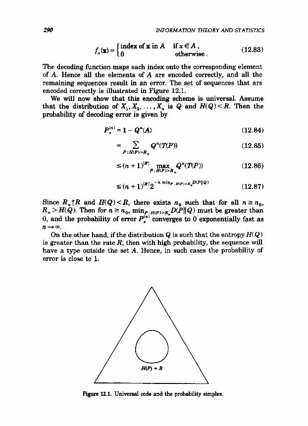
The decoding function maps each index onto the corresponding element of A. Hence all the elements of A are encoded correctly, and all the remaining sequences result in an error. The set of sequences that are encoded correctly is illustrated in Figure 12.1.

We will now show that this encoding scheme is universal. Assume that the distribution of XI, X,, . . . , X,, is Q and H(Q) CR. Then the probability of decoding error is given by

I’:’ = 1 - Q”(A) (12.84)

= c Q’VW) (12.85) P : H(P)>R,

I (n + 1)‘“’ max Q”(W)) P : H(P)>R,,

(12.86)

-=I (n + 1)‘“‘2 -n m%wP)>R”wIQ) - (12.87)

Since R, TR and H(Q) < R, there exists n, such that for all n L n,, R, > H(Q). Then for n 1 n,, minp,Htpl,Rno(PIIQ> must be greater than 0, and the probability of error Pr’ converges to 0 exponentially fast as n-a.

On the other hand, if the distribution Q is such that the entropy H(Q) is greater than the rate R, then with high probability, the sequence will have a type outside the set A. Hence, in such cases the probability of error is close to 1.

Figure 12.1. Universal code and the probability simplex.

12.4 LARGE DEVIATION THEORY 291

H(Q) Rate of code

Figure 12.2. Error exponent for the universal code.

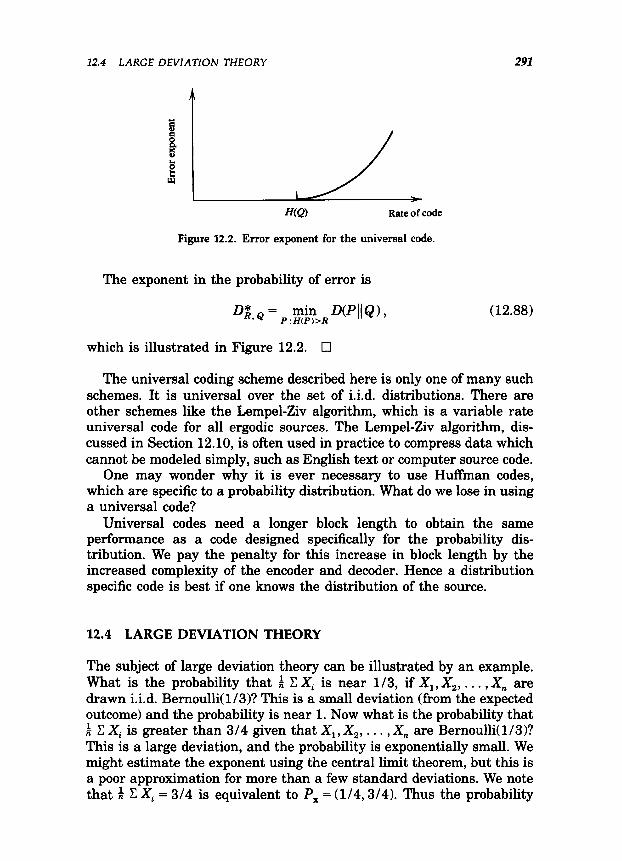
The exponent in the probability of error is

D&g = min DP((Q), P : H(P)>R

(12.88)

which is illustrated in Figure 12.2. Cl

The universal coding scheme described here is only one of many such schemes. It is universal over the set of i.i.d. distributions. There are other schemes like the Lempel-Ziv algorithm, which is a variable rate universal code for all ergodic sources. The Lempel-Ziv algorithm, discussed in Section 12.10, is often used in practice to compress data which cannot be modeled simply, such as English text or computer source code.

One may wonder why it is ever necessary to use Huffman codes, which are specific to a probability distribution. What do we lose in using a universal code?

Universal codes need a longer block length to obtain the same performance as a code designed specifically for the probability distribution. We pay the penalty for this increase in block length by the increased complexity of the encoder and decoder. Hence a distribution specific code is best if one knows the distribution of the source.

12.4 LARGE DEVIATION THEORY

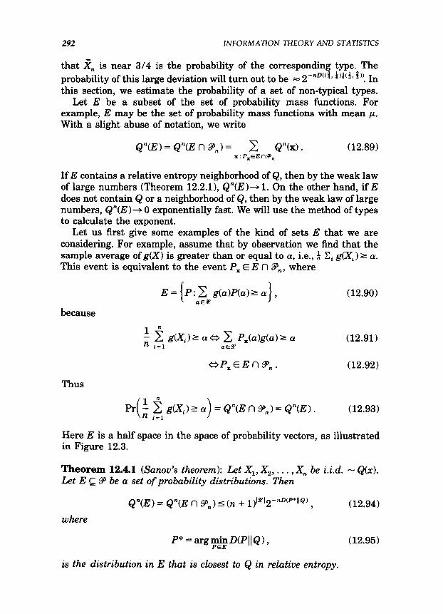
The subject of large deviation theory can be illustrated by an example. What is the probability that w C Xi is near l/3, if X1, X,, . . . , X, are drawn i.i.d. Bernoulli( l/3)? This is a small deviation (from the expected outcome) and the probability is near 1. Now what is the probability that k C Xi is greater than 3/4 given that X1, X,, . . . , X, are Bernoulli(l/3)? This is a large deviation, and the probability is exponentially small. We might estimate the exponent using the central limit theorem, but this is a poor approximation for more than a few standard deviations. We note that i C Xi = 3/4 is equivalent to P, = (l/4,3/4). Thus the probability

292 INFORMATION THEORY AND STATISTICS

that X, is near 3/4 is the probability of the corresponding type. The probability of this large deviation will turn out to be = 2 -nD(( lf f )‘I( f, % “! In this section, we estimate the probability of a set of non-typical types.

Let E be a subset of the set of probability mass functions. For example, E may be the set of probability mass functions with mean p. With a slight abuse of notation, we write

Q”(E) = Q”(E n 9’J = 2 Q”(x). x: P,EE~~,,

(12.89)

If E contains a relative entropy neighborhood of Q, then by the weak law of large numbers (Theorem 12.2.1), Q”(E)+ 1. On the other hand, if E does not contain Q or a neighborhood of Q, then by the weak law of large numbers, Q”(E )+ 0 exponentially fast. We will use the method of types to calculate the exponent.

Let us first give some examples of the kind of sets E that we are considering. For example, assume that by observation we find that the sample average of g(X) is greater than or equal to QI, i.e., k Ci g<x, > L ar. This event is equivalent to the event Px E E n P,, where

because

E = {P: 2 g(a)P(u)r a}, aE&

(12.90)

(12.91)

~P,EEM’~. (12.92)

Thus

(12.93)

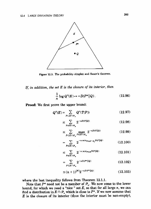
Here E is a half space in the space of probability vectors, as illustrated in Figure 12.3.

Theorem 12.4.1 (Sunov’s theorem): Let Xl, X2, . . . , X, be i.i.d. - Q(x). Let E c 9 be a set of probability distributions. Then

where

Q”(E) = Q”(E n 9,) 5 (n + ~)I*~~-~D(P*IIQ) ? (12.94)

P* = argyigD(PII&), (12.95)

is the distribution in E that is closest to Q in relative entropy.

12.4 LARGE DEVIATION THEORY 293

Figure 12.3. The probability simplex and Sanov’s theorem.

If, in addition, the set E is the closure of its interior, then

; log Qn(E)+ -D(P*llQ) . (12.96)

Proof: We first prove the upper bound:

Q”(E)= 2 Q”W-‘N PEEPS’,,

(12.97)

5 c 6pvPIlQ) (12.98)

PEEW,

5 c max 2 -nD(PllQ)

PEEr-9, PEEn9’,

(12.99)

= c 2 -n minpEEnpn~(PllQ) (12.100) PEEnp’,

I 2 2 -n minp&XP(lQ) (12.101) PEEnB,

= 2 spwJ*llQ) PEEn9,

(12.102)

< cn + ~~l~l2-~~(J’*llQ) (12.103)

where the last inequality follows from Theorem 12.1.1. Note that P* need not be a member of .Pn. We now come to the lower

bound, for which we need a “nice ” set E, so that for all large n, we can find a distribution in E n .P,, which is close to P. If we now assume that E is the closure of its interior (thus the interior must be non-empty),

294 INFORMATION THEORY AND STATISTZCS

then since U n 9,, is dense in the set of all distributions, it follows that E n 9n is non-empty for all n 1 n, for some n,. We can then fknd a sequence of distributions P,, such that P, E E n 9n and D(P, IIQ) +D(P*IIQ). For each n 2 n,,

Q”(E)= 2 &VW) PeErW,

1 Q”U’Pn ))

1 21 (n + lj”l

2-~~(P,llQ) .

Consequently,

(12.104)

(12.105)

(12.106)

1 lim inf ; log Q”(E) I lim i

IS?1 logh + 1) -

n

= -D(P*)lQ).

- D(P,llQ$

(12.107)

Combining this with the upper bound establishes the theorem. Cl

This argument can also be extended to continuous distributions using quantization.

12.5 EXAMPLES OF SANOV’S THEOREM

Suppose we wish to find Pr{ i Cy=, gj(X,> 2 a!, j = 1,2,. . . , k}. Then the set E is defined as

E = {P: 2 P(a)gj(a) 1 ~j, j = 1,2, . . . , k} . (12.108) a

To find the closest distribution in E to Q, we minimize D(PII Q) subject to the constraints in (12.108). Using Lagrange multipliers, we construct the functional

P(x) J(P) = c Rd log g<=c> + C Ai C P<x)gi(~> + VC p(~) . (12’log) x i x x

We then differentiate and calculate the closest distribution to Q to be of the form

P*(x) = Q(& ci %gi(x)

c a~&” Q(a)e”i *igi(a) ’ (12.110)

12.5 EXAMPLES OF SANOV’S THEOREM 295

where the constants Ai are chosen to satisfy the constraints. Note that if Q is uniform, then P* is the maximum entropy distribution. Verification that P* is indeed the minimum follows from the same kind of arguments as given in Chapter 11.

Let us consider some specific examples:

Example 12.5.1 (Dice): Suppose we toss a fair die n times; what is the probability that the average of the throws is greater than or equal to 4? From Sanov’s theorem, it follows that

Q”(E)& 2-P*llQJ , (12.111)

where P* minimizes D(PIIQ) over all distributions P that satisfy

$ iP(i)l4. i=l

From (12.110), it follows that P* has the form

2 p*w = g$ , z-l

(12.112)

(12.113)

with h chosen so that C iP*(i) = 4. Solving numerically, we obtain A=0.2519, and P*= (0.1031,0.1227,0.1461,0.1740,0.2072,0.2468), and therefore D(P*II Q) = 0.0624 bits. Thus, the probability that the average of 10000 throws is greater than or equal to 4 is = 2-624.

Example 12.62 (Coins): Suppose we have a fair coin, and want to estimate the probability of observing more than 700 heads in a series of 1000 tosses. The problem is like the previous example. The probability is

(12.114)

where P* is the (0.7,0.3) distribution and Q is the (0.5,0.5) distribution. In this case, D(P*IIQ) = 1 - H(P*) = 1 - H(0.7) = 0.119. Thus th;lgprobability of 700 or more heads in 1000 trials is approximately 2- .

Example 12.6.3 (Mutual dependence): Let Q(x, y) be a given joint distribution and let QJx, y) = Q(x>Q( y) be the associated product distribution formed from the marginals of Q. We wish to know the likelihood that a sample drawn according to Q0 will “appear” to be jointly distributed according to Q. Accordingly, let (Xi, Yi) be i.i.d. -Q&, y)= Q(x)&(y). W e d fi e ne joint typicality as we did in Section 8.6,

296 INFORMATlON THEORY AND STATISTICS

i.e., (x”, y”) is jointly typical with respect to a joint distribution Q(x, y) iff the sample entropies are close to their true values, i.e.,

-i log&(x")-H(x) SE, (12.115)

+ogQ(y”)-H(Y) SE, (12.116)

and

1 -,logQ(x”,y”)-H(X,Y) SE. (12.117)

We wish to calculate the probability (under the product distribution) of seeing a pair (x”, y”) that looks jointly typical of Q, i.e., (x”, y”) satisfies (12.115)-(12.117). Thus (x”, y”) are jointly typical with respect to Q(x, y) if P xn, yn E E n iFn (X, Y), where

E= - 2 P(x, y) log Q(x) - H(X) 5 E , x9 Y

-c Rx, y) log Q(y) - H(Y) 5 E , x* Y

-c P(x, y) log Q(x, y) - H(X, Y) . (12.118) x9 Y

Using Sanov’s theorem, the probability is

Q;(E) & 2-n~(p*!lQ,) , (12.119)

where P* is the distribution satisfying the constraints that is closest to Q0 in relative entropy. In this case, as E + 0, it can be verified (Problem 10) that P* is the joint distribution Q, and Q0 is the product distribution, so that the probability is 2-nDcQcX9 y)ttQ(x)Q(y)) = 2-nrcXi y’, which is the same as the result derived in Chapter 8 for the joint AEP

In the next section, we consider the empirical distribution of the sequence of outcomes given that the type is in a particular set of distributions E. We will show that not only is the probability of the set E essentially determined by D(P*II Q), the distance of the closest element of E to Q, but also that the conditional type is essentially P*, so that given that we are in set E, the type is very likely to be close to P*.

12.6 THE CONDZTZONAL LlMlT THEOREM 297

12.6 THE CONDITIONAL LIMIT THEOREM

It has been shown that the probability of a set of types under a distribution Q is essentially determined by the probability of the closest element of the set to Q; the probability is 2-nD* to first order in the exponent, where

D” = yn; D(PllQ) . (12.120)

This follows because the probability of the set of types is the sum of the probabilities of each type, which is bounded by the largest term times the number of terms. Since the number of terms is polynomial in the length of the sequences, the sum is equal to the largest term to first order in the exponent.

We now strengthen the argument to show that not only is the probability of the set E essentially the same as the probability of the closest type P* but also that the total probability of other types that are far away from P* is negligible. This implies that with very high probability, the observed type is close to P*. We call this a conditional limit theorem.

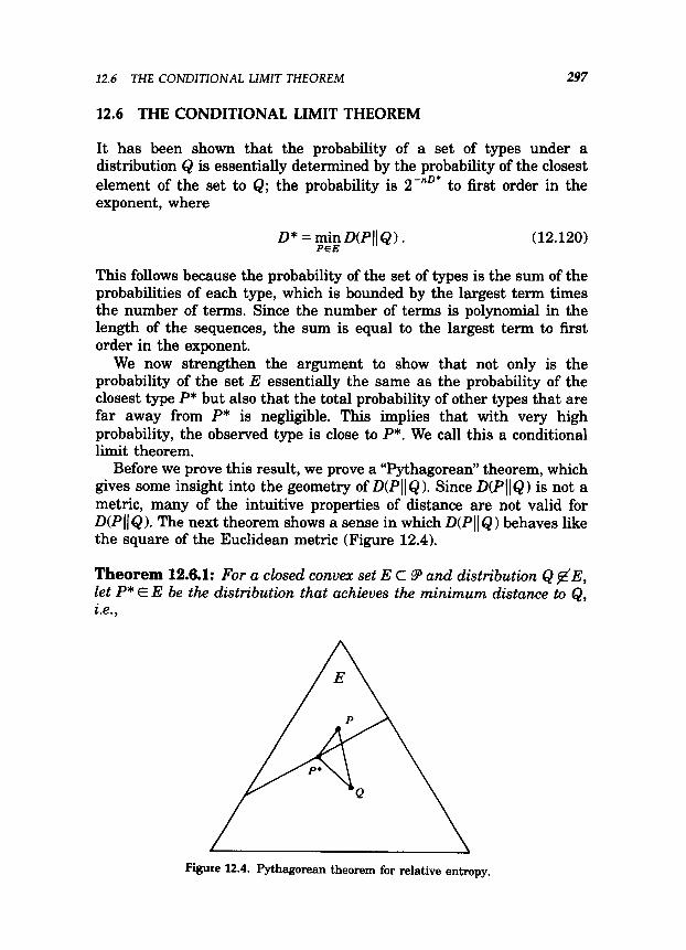
Before we prove this result, we prove a “Pythagorean” theorem, which gives some insight into the geometry of D(P 11 Q ). Since D(P 11 Q ) is not a metric, many of the intuitive properties of distance are not valid for D(P(lQ). The next theorem shows a sense in which D(PIIQ) behaves like the square of the Euclidean metric (Figure 12.4).

Theorem 12.6.1: For a closed convex set E C 9 and distribution Q $E, let P* E E be the distribution that achieves the minimum distance to Q, i.e.,

Figure 12.4. Pythagorean theorem for relative entropy.

298 1NFORMATlON THEORY AND STATKTZCS

Then

for all P E E.

D(P(IQ)rD(PIIP*)+D(P*I(Q) (12.122)

Note: The main use of this theorem is as follows: suppose we have a sequence P, E E that yields D(P, II Q ) + D(P* II Q 1. Then from the Py- thagorean theorem, D(P, II P*)+ 0 as well.

Proof: Consider any P E E. Let

PA = AP + (1 - A)P* . (12.123)

Then PA + P* as A + 0. Also since E is convex, PA E E for 0 I A I 1. Since D(P*IlQ) is the minimum of D(P,IIQ) along the path P*+P, the derivative of D(P, I I Q ) as a function of A is non-negative at A = 0. Now

P,(x) D,=D(P,IIQ)=C.P,(z)logQo, (12.124)

d4 -= dh (Rx) - P”(x)) log g + (P(x) - P*(x))) .

X (12.125)

Setting A = 0, so that PA = P* and using the fact that C P(x) = C P*(x) = 1, we have

= 2 (P(x) - P”(x)) log $+ X

= 2 P(x) log $L$ - c P*‘(x) log p+ X

= 2 P(x) log z s - c P*(x) log z X

= DU’((Q) - D(P(IP*) - DP*llQ>,

which proves the theorem. Cl

(12.126)

(12.127)

(12.128)

(12.129)

(12.130)

12.6 THE CONDITIONAL LZMlT THEOREM 299

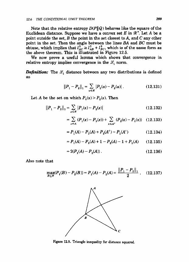
Note that the relative entropy D(PII Q) behaves like the square of the Euclidean distance. Suppose we have a convex set E in % n. Let A be a point outside the set, B the point in the set closest to A, and C any other point in the set. Then the angle between the lines BA and BC must be obtuse, which implies that Zic 1 IL + I&, which is of the same form as the above theorem. This is illustrated in Figure 12.5.

We now prove a useful lemma which shows that convergence in relative entropy implies convergence in the ZI norm.

The .ZI distance between any two distributions is defined

Let A be the set on which P,(X) > P&G). Then

lp$ - Pz 111 = c IP&) - P&)1 xE&

Also note that

= c P,(r) - P,(x)> + c (P&d - P,(x)> XEA ZEAC

= P,(A) - P,(A) + &(A”) - &(A”)

= P,(A) -P,(A) + 1 -P,(A) - 1 + P,(A)

= W,(A) - P,(A)) .

(12.131)

(12.132)

(12.133)

(12.134)

(12.135)

(12.136)

(12.137)

Figure 12.5. Triangle inequality for distance squared.

300 INFORMATlON THEORY AND STATZSTZCS

The left hand side of (12.137) is called the variational distance between PI and Pz.

Lemma 12.6.1:

(12.138)

Proof: We first prove it for the binary case. Consider two binary distributions with parameters p and q with p 1 q. We will show that

l-p 4 plog~+(l-p)logi_g~~(P-q)2~ (12.139)

The difference g(p, q) between the two sides is

l-p 4 g~p,q)=Plog~+u-p)log--

1-q m(P - d2 *

(12.140)

Then

dg(P,d P 1-P 4 dq -- = qln2

+ (1 -q)ln2 - g&Kq -p) (12.141)

Q-P 4 = q(l- q)ln2 - &I -P) (12.142)

10 9 (12.143)

since q(1 - q) 5 f and q 5 p. For q = p, g(p, q) = 0, and hence g( p, q) 2 0 for q 5 p, which proves the lemma for the binary case.

For the general case, for any two distributions P, and P2, let

A = {x: PI(x) > P,(x)} . (12.144)

Define a new binary random variable Y = 4(X), the indicator of the set A, and let P, and P2 be the distributions of Y. Thus P, and P, correspond to the quantized versions of P, and P,. Then by the data processing inequality applied to relative entropies (which is proved in the same way as the data processing inequality for mutual information), we have

(12.145)

(12.146)

12.6 THE CONDITIONAL LlMlT THEOREM 301

= & IlPl - PzllT (12.147)

by (12.137), and the lemma is proved. Cl

We can now begin the proof of the conditional limit theorem. We first outline the method used. As stated at the beginning of the chapter, the essential idea is that the probability of a type under Q depends exponentially on the distance of the type from Q, and hence types that are further away are exponentially less likely to occur. We divide the set of types in E into two categories: those at about the same distance from Q as P* and those a distance 26 farther away. The second set has exponentially less probability than the first, and hence the first set has a conditional probability tending to 1. We then use the Pythagorean theorem to establish that all the elements in the first set are close to P*, which will establish the theorem.

The following theorem is an important strengthening of the maximum entropy principle.

Theorem 12.6.2 (Conditional limit theorem): Let E be a closed convex subset of 9 and let Q be a distribution not in E. Let XI, X2, . . . , X, be discrete random variables drawn i.i.d. -Q. Let P* achieve min,,, WP(IQ). Then

Pr(x, = alPxn E E)+ P*(a) (12.148)

in probability as n + 00, i.e., the conditional distribution of XI, given that the type of the sequence is in E, is close to P* for large n.

Example 12.6.1: If Xi i.i.d. - Q, then

where P*(a) minimizes D(PIJQ) over P satisfying C P(a)a2 1 a. This minimization results in

ha2

P*(a) = Q(a) e C, Q(a)eAa2 ’

(12.150)

where A is chosen to satisfy C P*(a)a2 = CL Thus the conditional distribution on X1 given a constraint on the sum of the squares is a (normalized) product of the original probability mass function and the maximum entropy probability mass function (which in this case is Gaussian).

302 ZNFORMATZON THEORY AND STATISTICS

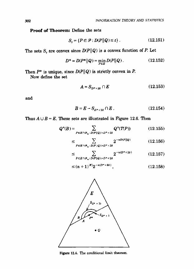
Proof of Theorem: Define the sets

S, = {PE cP:D(PIlQ)st}. (12.151)

The sets S, are convex since D(P 11 Q ) is a convex function of P. Let

D* = D(P*IIQ) = pE~D(PllQ). (12.152)

Then P* is unique, since D(P II Q ) is strictly convex in I? Now define the set

A = SDefz6 n E (12.153)

and

B=E-S,,,,,nE. (12.154)

Thus A U B = E. These sets are illustrated in Figure 12.6. Then

Q”(B) = PEE”~‘, :&,Q,>o.+26 QvYP)) (12.155)

I c ywllQ) (12.156) PEEW, :D(PllQ)>D*+26

I c 2 -n(D*+2s) (12.157) PEEM’,:D(PJJQ)>D*+2S

< cn + 1)1&“12-4D*+2~) - 9 (12.158)

Figure 12.6. The conditional limit theorem.

12.6 THE CONDITZONAL LlMlT THEOREM 303

since there are only a polynomial number of types. On the other hand,

Q"(A) 2 &"CS,.+, n E) (12.159)

= (12.160)

c 1 1 PEEn9, :DG’llQ)sD*+6 (?Z + l)‘*’

yW’11Q) (12.161)

1 2 (n + 1)‘“’

2- n(D*+S) ’ for n sufficiently large , (12.162)

since the sum is greater than one of the terms, and for sufficiently large n, there exists at least one type in SD*+6 n E fl 9,. Then for n sufficiently large

I Q"(B) Q”(A)

(12.163)

(12.164)

I (n + l)l&“l2-dD*+w

&2- n(D*+6) (12.165)

= (n + l)2iz12-n6 ’ (12.166)

which goes to 0 as n --* m. Hence the conditional probability of B goes to 0 as n + 00, which implies that the conditional probability of A goes to 1.

We now show that all the members of A are close to P* in relative entropy. For all members of A,

D(PIlQ)5D*+26. (12.167)

Hence by the “Pythagorean” theorem (Theorem 12.6.1))

D(pIIP*) + D(P*IlQ) 5 D(Pl(Q) 5 D* + 2s , (12.168)

which in turn implies that

D(PJ(P”) 5 2s ) (12.169)

since D(P*(I Q) = D*. Thus P, E A implies that D(P,II Q) 5 D* + 26, and therefore that D(P,IIP*) I 28. Consequently, since Pr{P,, E A(P,, E E} --) 1, it follows that

304 INFORMATION THEORY AND STATZSTZCS

Pr(D(P,,IIP”)I2SIP,,EE)-,l (12.170)

By Lemma 12.6.1, the fact that the relative entropy is small implies that the 3, distance is small, which in turn implies that max,,zt” ppw - P”(a>l is small. Thus Pr(IP,,(a) - P*(a)) 2 EIP,, E E)+ 0 as n + 00. Alternatively, this can be written as

Pr(x, = a IPxn E E) + P*(a) in probability . (12.171)

In this theorem, we have only proved that the marginal distribution goes to P* as n --) co. Using a similar argument, we can prove a stronger version of this theorem, i.e.,

m

Pr(x, = u,,X, = uz,. . . ,x, = u,lPp EE)+ n P”(u,) in probability . i=l

(12.172)

This holds for fked m as n + 00. The result is not true for m = n, since there are end effects; given that the type of the sequence is in E, the last elements of the sequence can be determined from the remaining elements, and the elements are no longer independent. The conditional limit theorem states that the first few elements are asymptotically independent with common distribution P*.

Example 12.6.2: As an example of the conditional limit theorem, let us consider the case when n fair dice are rolled. Suppose that the sum of the outcomes exceeds 4n. Then by the conditional limit theorem, the probability that the first die shows a number a E { 1,2, . . . ,6} is approximately P*(u), where P*(u) is the distribution in E that is closest to the uniform distribution, where E = {P: C P(u)u 14). This is the maximum entropy distribution given by

2 p*w = & , i-l

(12.173)

with A chosen so that C iP*(i) = 4 (see Chapter 11). Here P* is the conditional distribution on the first (or any other) die. Apparently the first few dice inspected will behave as if they are independently drawn according to an exponential distribution.

12.7 HYPOTHESIS TESTING

One of the standard problems in statistics is to decide between two alternative explanations for the observed data. For example, in medical

12.7 HYPOTHESlS TESTZNG 305

testing, one may wish to test whether a new drug is effective or not. Similarly, a sequence of coin tosses may reveal whether the coin is biased or not.

These problems are examples of the general hypothesis testing problem. In the simplest case, we have to decide between two i.i.d. distributions. The general problem can be stated as follows:

Problem: Let X, , X,, . . . , X,, be i.i.d. - Q(Z). We consider two hypotheses:

l H,: Q=P,.

l H2:Q=P2.

Consider the general decision function g(xl, xs, . . . , x, ), where g&9 x2, * * * 9 XJ = 1 implies that HI is accepted and g(+ x2, . . . , xn) = 2 implies that H, is accepted. Since the function takes on only two values, the test can also be specified by specifying the set A over which &Xl, 372, * * * 2 x,J is 1; the complement of this set is the set where gb,, 3t2, * * * 9 rn ) has the value 2. We define the two probabilities of error:

a = Pr<g(X,,X,, . . . , X,) = 21H, true) = Py(A”) (12.174)

and

p = pr(g(x,,x,, * * * , X,) = 11H2 true) = Pi(A). (12.175)

In general, we wish to minimize both probabilities, but there is a trade-off. Thus we minimize one of the probabilities of error subject to a constraint on the other probability of error. The best achievable error exponent in the probability of error for this problem is given by Stein’s lemma.

We first prove the Neyman-Pearson lemma, which derives the form of the optimum test between two hypotheses. We derive the result for discrete distributions; the same results can be derived for continuous distributions as well.

Theorem 12.7.1 (Neyman-Pearson lemma): Let Xl, X2, . . . ,X, be drawn i.i.d. according to probability mass function P Consider the decision problem corresponding to hypotheses Q = PI vs. Q = P2. For T 2 0, define a region

(12.176)

Let

a* = P;(A”,(T)), p* = P&4,(T)), (12.177)

306 INFORMATION THEORY AND STATZSTZCS

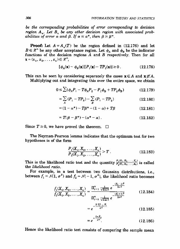
be the corresponding probabilities of error corresponding to decision region A,. Let B, be any other decision region with associated probabilities of error C-X and p. If a 5 a*, then p L p*.

Proof: Let A = A,(T) be the region defined in (12.176) and let B E 35’” be any other acceptance region. Let $Q and 4B be the indicator functions of the decision regions A and B respectively. Then for all x=(x1,x2 ,..., xJE2rn,

h/&d - ~&dlP,(x> - Tp,(X)l~ 0 l (12.178)

This can be seen by considering separately the cases x E A and xeA. Multiplying out and integrating this over the entire space, we obtain

=zP,-TP,)-aP,-TP,) (12.180) A B

=(l-o!*)-Tp*-(l-cw)+Tp (12.181)

= T(p - p*) -(a* - a). (12.182)

Since T 2 0, we have proved the theorem. Cl

The Neyman-Pearson lemma indicates that the optimum test for two hypotheses is of the form

(12.183)

This is the likelihood ratio test and the quantity :i::z:::: $1 is called the likelihood ratio.

For example, in a test between two Gaussian distributions, i.e., between f, = .@l, a2> and f, = JV( - 1, 02), the likelihood ratio becomes

(Xi-1j2

f,<x,,X,, . . . ,x,> T=l & e 2az f2WpX2, ’ * * 9x,) = (Xi+l12

l-l;.-, * e 2u2

2 Cr=l Xi +-

=e cl2

(12.184)

(12.185)

+s =e cr.2 . (12.186)

Hence the likelihood ratio test consists of comparing the sample mean

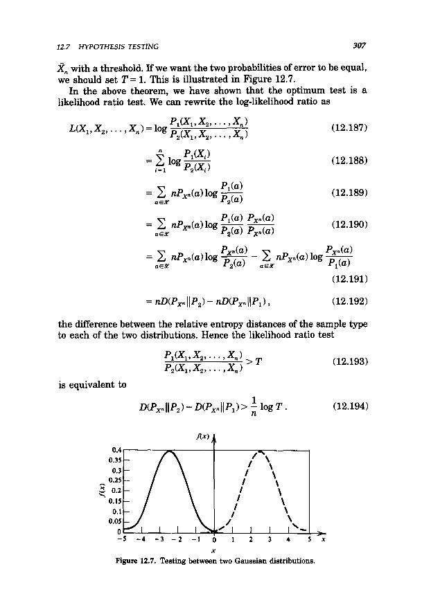
12.7 HYPOTHESIS TESTZNG 307

rl, with a threshold. If we want the two probabilities of error to be equal, we should set 2’ = 1. This is illustrated in Figure 12.7.

In the above theorem, we have shown that the optimum test is a likelihood ratio test. We can rewrite the log-likelihood ratio as

= 2 nP,,(a) log E aE&0 2

= 2 nP,,(a) log $$ x aEX Xn

(12.187)

(12.188)

(12.189)

(12.190)

= C nPxnW log p2(a) aE%

EE@ - C nP,,(U) log E aE& 1

(12.191)

= n~(P,,((P,) - nD(P,,((P,), (12.192)

the difference between the relative entropy distances of the sample type to each of the two distributions. Hence the likelihood ratio test

0.4 0.35

0.3 0.25

G 0.2 ST

0.15

0.1 0.05

0

1 // 1 ’ // ’

I : / ’ : I I I \ \

I’ I’ \ \ \ \

: :

\ \

*/ 1 */ 1 I ;\ -5-4-3-2-10 12 3 4 ,5 -4 -3 -2 -1 O 1 2 3 4 5x

X

Figure 12.7. Testing between two Gaussian distributions. X

Fi igure 12.7. Testing between two Gaussian distribut

is equivalent to

(12.193)

(12.194)


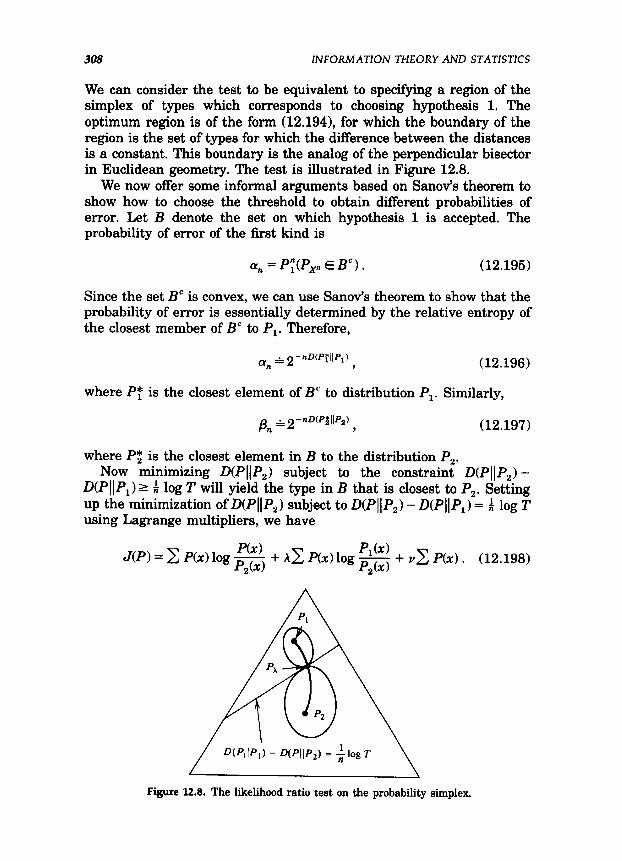
We can consider the test to be equivalent to specifying a region of the simplex of types which corresponds to choosing hypothesis 1. The optimum region is of the form (12.1941, for which the boundary of the region is the set of types for which the difference between the distances is a constant. This boundary is the analog of the perpendicular bisector in Euclidean geometry. The test is illustrated in Figure 12.8.

We now offer some informal arguments based on Sanov’s theorem to show how to choose the threshold to obtain different probabilities of error. Let B denote the set on which hypothesis 1 is accepted. The probability of error of the first hind is

%a = PycPp E B”) . (12.195)

Since the set B” is convex, we can use Sanov’s theorem to show that the probability of error is essentially determined by the relative entropy of the closest member of B” to P,. Therefore,

% ‘2-- nmqp~)

9 (12.196)

where PT is the closest element of B” to distribution PI. Similarly,

pn &2- nmq IlP~) 9 (12.197)

where Pz is the closest element in B to the distribution P,. Now minimizing D(PIIP,) subject to the constraint D(PIIP,) -

D(P(( PI) 2 A log T will yield the type in B that is closest to P2. Setting up the minimization of D(PIIP,) subject to D(PIIP,) - D(P)IP,) = $ log T using Lagrange multipliers, we have

Rx) J(P) = 2 P(x) log p + AC Rx) log p p1(=c) + vc P(x). (12.198) 2 2

Figure 12.8. The likelihood ratio test on the probability simplex.

12.8 STEIN’S LEMMA

Differentiating with respect to P(X) and setting to 0, we have

log %) Pl(=G)

P&d -+v=o. + 1+ A loI3 p&) (12.199)

Solving this set of equations, we obtain the minimizing P of the form

(12.200)

where A is chosen so that D(P,, 11 PI ) - D(P,, 11 Pz> = v. From the symmetry of expression (12.200), it is clear that PT = PX

and that the probabilities of error behave exponentially with exponents given by the relative entropies D(P*lI PI) and D(P*ll P2). Also note from the equation that as h + 1, Pn + P, and as A+ 0, PA + Pz. The line that PA traces out as h varies is a geodesic in the simplex. Here PA is a normalized convex combination, where the combination is in the exponent (Figure 12.8).

In the next section, we calculate the best error exponent when one of the two types of error goes to zero arbitrarily slowly (Stein’s lemma). We will also minimize the weighted sum of the two probabilities of error and obtain the Chernoff bound.

12.8 STEIN’S LEMMA

We now consider the case when one of the probabilities of error is fixed and we wish to minimize the other probability of error. The best error exponent in this case is given by Stein’s lemma.

Theorem 12.8.1 (Stein’s lemma): Let Xl, X2, . . . , X,, be i.i.d. - Q. Con- sider the hypothesis test between two alternatives, Q = PI and Q = Pz, where DP,I(p,)< 00. Let A, c P be an acceptance region for hypothesis 1. Let the probabilities of ermr be

a, = Py(Ae,) , pn =Pi(An) l (12.201)

and for O<E<& define

El= min &. A,W”

(12.202) U,<C

Then

(12.203)

310 INFORMATION THEORY AND STATISTICS

Proofi To prove the theorem, we construct a sequence of acceptance regions A, c Sep” such that (x,, < (E and 6,, k 2-“D’p”‘P2! We then show that no other sequence of tests has an asymptotically better exponent.

First, we define

A, = xEBY:2 +nux4(IP2)-6) ( P,(x) (2 - P&d -

Then we have the following properties:

1. Py(A,)+ 1. This follows from

P;ca,,l=f’;(; 8 ‘ogp i-l

p1w E(D(P,((P,)- s,D(PJP,)+ s,) 2 i

(12.205)

-,l (12.206)

by the strong law of large numbers, since DP, llP2) =

I!&+, (log s). Hence for sufficiently large n, a, < E.

2. Pi(A,) 5 2-n(D(PlllP2)? Using the definition of A,, we have

P;(A, I= c P,(x) *?a

I C p1(x)2-n(~‘P’Il%)-6)

4

= 2 -n(D(P111P2)-S) c P,(x)

*Ia

= 2--n(D(P~IIW-a)(1 _ a n

1.

Similarly, we can show that

Hence

P;(A,,)r2 -n(D(P11(P2)+G 1 Cl- a, ) l

1 logtl - an) ;logP,I -D(p,IIP,)+S+ n ,

and

1 i logBra

log(1 - ar,) -wqp,b-~+ n 9

(12.207)

(12.208)

(12.209)

(12.210)

(12.211)

(12.212)

(12.213)

12.8 STEIN’S LEMMA 311

1 lim $+i ; log Pn = - D(P,IIP,) . (12.214)

3. We now prove that no other sequence of acceptance regions does better. Let B, c %‘” be any other sequence of acceptance regions with cy,, B = Py(BC,) < E. Let &B, = Pi@,). We will show that

Pn,B 22 -kD(P,((P,kE) .

H”ere

P n, 4, =P~(B,)~P~(An’B,) (12.215)

= c P,(x) A”*Bn

= C pl~x)2-n(~(P’IIP,)+~)

An”Bn

(12.216)

(12.217)

= 2 -nuw,((P2)+S 1 c Pi(x) (12.218) A,“Bn

z(l - (y, - cy,, Bn)2-n(D(p1i’p2)+*) , (12.219)

where the last inequality follows from the union of events bound as follows:

(12.220)

(12.221)

'l-PICA',)-P,(B",) (12.222)

1 -$og&,5 -HP,IIP,)-a- log(l - an - an, 8,)

9 (12.224) n

and since 6 > 0 is arbitrary,

(12.225)

Thus no sequence of sets B, has an exponent better than D(P, IIP,). But the sequence A, achieves the exponent D(P, I(P,). Thus A, is asymptotically optimal, and the best error exponent is D(P, 11 P&. 0


12.9 CHERNOFF BOUND

We have considered the problem of hypothesis testing in the classical setting, in which we treat the two probabilities of error separately. In the derivation of Stein’s lemma, we set a, I E and achieved 6, * 2-“4 But this approach lacks symmetry. Instead, we can follow a Bayesian approach, in which we assign prior probabilities to both the hypotheses. In this case, we wish to minimize the overall probability of error given by the weighted sum of the individual probabilities of error. The resulting error exponent is the Chernoff information.

The setup is as follows: X1, X,, . . . , X, i.i.d. - Q. We have two hypotheses: Q = P, with prior probability w1 and Q = P, with prior probability rr2. The overall probability of error is

P;’ = ?r,ar, + nip, . (12.226)

Let

1 D* = !.i+.iArnz” - ; log PF’ . (12.227)

R

Theorem 12.9.1 (Chenwff): The best achievable exponent in the Bayesian probability of error is D*, where

D* = D(P#l) = D(P,*IIP,), (12.228)

with

(12.229)

and A* the value of A such that

D(p,#‘,) = W’,~IIP,) . (12.230)

Proof: The basic details of the proof were given in the previous section. We have shown that the optimum test is a likelihood ratio test, which can be considered to be of the form

D(P~rllP~)-D(P,,llP,)> 2’. (12.231)

The test divides the probability simplex into regions corresponding to hypothesis 1 and hypothesis 2, respectively. This is illustrated in Figure 12.9.

Let A be the set of types associated with hypothesis 1. From the

12.9 CHERNOFF BOUND 313

Figure 12.9. The probability simplex and Chernoffs bound.

discussion preceding (12.200), it follows that the closest point in the set A” to P, is on the boundary of A, and is of the form given by (12.229). Then from the discussion in the last section, it is clear that PA is the distribution in A that is closest to P2; it is also the distribution in A” that is closest to P,. By Sanov’s theorem, we can calculate the associated probabilities of error

and ff?l

= plf(AC)&2-nD(p~*11P1)

p, = p;(A) & 2 -nD(P~*11P2) .

(12.232)

(12.233)

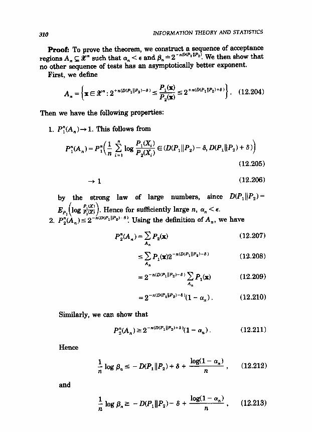
In the Bayesian case, the overall probability of error is the weighted sum of the two probabilities of error,

since the exponential rate is determined by the worst exponent. Since D(P, 11 PJ increases with A and D(P, 11 Pz) decreases with A, the maximum value of the minimum of {D(P, II P, ), D(P, II P, >} is attained when they are equal. This is illustrated in Figure 12.10.

Hence, we choose A so that

WqlP,) = D(P*IIP,) i C(P,, PSI. (12.235)

Thus C(P,, Pz> is the highest achievable exponent for the probability of error and is called the Chernoff information. Cl

The above definition is equivalent to the standard definition of Chernoff information,

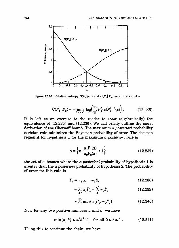
314 lNFORMATlON THEORY AND STATZSTKS

Figure 12.10. Relative entropy D(P,IJP,) and D(P,(IP,) as a function of A.

(12.236)

It is left as an exercise to the reader to show (algebraically) the equivalence of (12.235) and (12.236). We will briefly outline the usual derivation of the Chernoff bound. The maximum a posteriori probability decision rule minimizes the Bayesian probability of error. The decision region A for hypothesis 1 for the maximum a posteriori rule is

?r P (d A={x:-&>l (12.237)

the set of outcomes where the a posteriori probability of hypothesis 1 is greater than the a posteriori probability of hypothesis 2. The probability of error for this rule is

P, = Tl% + 48 (12.238)

(12.239)

= C min{ n,P,, r2P,} . (12.240)

Now for any two positive numbers a and 6, we have

min{a, b} sa*b’-*, for all 0~ AS 1. (12.241)

Using this to continue the chain, we have


P, = C min{ qP,, ?r,P,) (12.242)

(12.243)

5 c P;P;-̂ . (12.244)

For a sequence of i.i.d. observations, Pk(x) = II:= 1 Pk(xi ), and

(12.245)

(12.246)

(12.247)

= (c P:P:-^)’ , where (a) follows since rI 5 1, 7~~ I 1. Hence, we have

i log Py 5 log c P;(x)P;-A(x)

(12.248)

(12.249)

Since this is true for all A, we can take the minimum over 0 I h I 1, resulting in the Chernoff bound. This proves that the exponent is no better than C(P,, P,>. Achievability follows from Theorem 12.9.1.

Note that the Bayesian error exponent does not depend on the actual value of ?rI and rZ, as long as they are non-zero. Essentially, the effect of the prior is washed out for large sample sizes. The optimum decision rule is to choose the hypothesis with the maximum a posteriori probability, which corresponds to the test

(12.250)

Taking the log and dividing by n, this test can be rewritten as

1 P,(x-1 ;1og3+---log&JsO,

r2 i 2 i (12.251)

where the second term tends to D(P, IIP,> or - D(P, IIP,> accordingly as PI or P2 is the true distribution. The first term tends to 0, and the effect of the prior distribution washes out.

Finally, to round off our discussion of large deviation theory and hypothesis testing, we consider an example of the conditional limit theorem.

316 ZNFORMATZON THEORY AND STATISTKS

Example 12.9.1: Suppose major league baseball players have a batting average of 260 with a standard deviation of 15 and suppose that minor league ballplayers have a batting average of 240 with a standard deviation of 15. A group of 100 ballplayers from one of the leagues (the league is chosen at random) is found to have a group batting average greater than 250, and is therefore judged to be major leaguers. We are now told that we are mistaken; these players are minor leaguers. What can we say about the distribution of batting averages among these 100 players? It will turn out that the distribution of batting averages among these players will have a mean of 250 and a standard deviation of 15. This follows from the conditional limit theorem. To see this, we abstract the problem as follows.

Let us consider an example of testing between two Gaussian distributions, fi = Crr(l, a2> and f, = JV( - 1, 02), with different means and the same variance. As discussed in the last section, the likelihood ratio test in this case is equivalent to comparing the sample mean with a threshold. The Bayes test is “Accept the hypothesis f = f, if a Cr=, Xi > 0.”

Now assume that we make an error of the first kind (we say f = f, when indeed f = f,> in this test. What is the conditional distribution of the samples given that we have made an error?

We might guess at various possibilities:

l The sample will look like a ( $, 4 ) mix of the two normal distributions. Plausible as this is, it is incorrect.

. Xi = 0 for all i. This is quite clearly very very unlikely, although it is conditionally likely that X, is close to 0.

l The correct answer is given by the conditional limit theorem. If the true distribution is f, and the sample type is in the set A, the conditional distribution is close to f*, the distribution in A that is closest to f,. By symmetry, this corresponds to A = 4 in (12.229). Calculating the distribution, we get

f*(x) = ( 1 (*-1J2 l/2 --

m e 2u2 > (

1 (x+1j2 l/2 --

m e 2c72 >

I( 1 (x-1J2 l/2 -- > ( 1 (z+1j2 l/2 --

m e 2=2 m e 2u2 dx >

1 -- (x2+1)

m e 2u2

= I 1 -- (x2+1)

m e 202 dx

(12.252)

(12.253)


1 -- =-

+j&3 e zcz2 (12.254)

= h-(0, (r2). (12.255)

It is interesting to note that the conditional distribution is normal with mean 0 and with the same variance as the original distributions. This is strange but true; if we mistake a normal population for another, the “shape” of this population still looks normal with the same variance and a different mean. Apparently, this rare event does not result from bizarre looking data.

Example 12.9.2 (Large deviation theory and football): Consider a very simple version of football in which the score is directly related to the number of yards gained. Assume that the coach has a choice between two strategies: running or passing. Associated with each strategy is a distribution on the number of yards gained. For example, in general, running results in a gain of a few yards with very high probability, while passing results in huge gains with low probability. Examples of the distributions are illustrated in Figure 12.11.

At the beginning of the game, the coach uses the strategy that promises the greatest expected gain. Now assume that we are in the closing minutes of the game and one of the teams is leading by a large margin. (Let us ignore first downs and adaptable defenses.) So the trailing team will win only if it is very lucky. If luck is required to win, then we might as well assume that we will be lucky and play accordingly. What is the appropriate strategy?

Assume that the team has only n plays left and it must gain I yards, where Z is much larger than n times the expected gain under each play. The probability that the team succeeds in achieving I yards is exponentially small; hence, we can use the large deviation results and Sanov’s theorem to calculate the probability of this event.

Yards gained in pass Yards gained in run

Figure 12.11. Distribution of yards gained in a run or a pass play.

318 1NFORMATlON THEORY AND STATISTKS

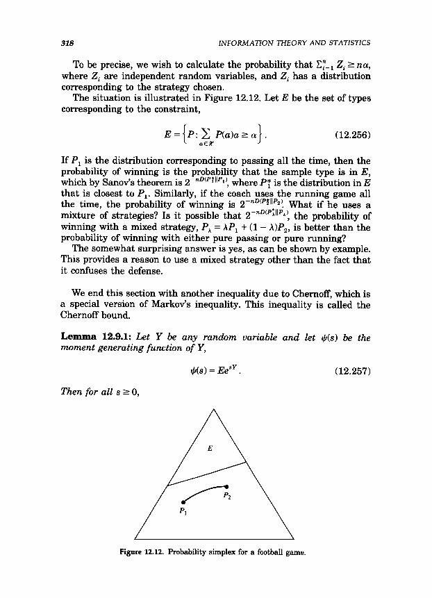
To be precise, we wish to calculate the probability that Cy= 1 Zi 1 ncx, where Zi are independent random variables, and Zi has a distribution corresponding to the strategy chosen.

The situation is illustrated in Figure 12.12. Let E be the set of types corresponding to the constraint,

E={P: 2 Papa}. aE%

(12.256)

If P, is the distribution corresponding to passing all the time, then the probability of winning is the probability that the sample type is in E, which by Sanov’s theorem is 2-nD(PT”P1), where PT is the distribution in E that is closest to P,. Similarly, if the coach uses the running game all the time, the probability of winning is 2-RD(p5”p2! What if he uses a mixture of strategies? Is it possible that 2-nD(P;“PA), the probability of winning with a mixed strategy, PA = AP, + (1 - h)P,, is better than the probability of winning with either pure passing or pure running?

The somewhat surprising answer is yes, as can be shown by example. This provides a reason to use a mixed strategy other than the fact that it confuses the defense.

We end this section with another inequality due to Chernoff, which is a special version of Markov’s inequality. This inequality is called the Chernoff bound.

Lemma 12.9.1: Let Y be any random variable and let e(s) be the moment generating function of Y,

+5(s) = Eesy .

Then for all s 2 0,

Figure 12.12. Probability simplex for a football game.

12.10 LEMPEL-ZN CODING 319

Proofi able es7

APPlY cl

Pr(Y L a) I e-““+(s) . (12.258)

Markov’s inequality to the non-negative random vari-

12.10 LEMPEL-ZIV CODING

We now describe a scheme for universal data compression due to Ziv and Lempel [291], which is simple to implement and has an asymptotic rate approaching the entropy of the source. The algorithm is particularly simple and has become popular as the standard algorithm for file compression on computers because of its speed and efficiency.

We will consider a binary source throughout this section. The results generalize easily to any finite alphabet.

Algorithm: The source sequence is sequentially parsed into strings that have not appeared so far. For example, if the string is 1011010100010.. . , we parse it as 1,0,11,01,010,00,10,. . . . After every comma, we look along the input sequence until we come to the shortest string that has not been marked off before. Since this is the shortest such string, all its prefixes must have occurred earlier. In particular, the string consisting of all but the last bit of this string must have occurred earlier. We code this phrase by giving the location of the prefix and the value of the last bit.

Let c(n) be the number of phrases in the parsing of the input n-sequence. We need log c(n) bits to describe the location of the prefix to the phrase and 1 bit to describe the last bit. For example, the code for the above sequence is (OOO,l)(OOO,O)(OOl,l)(OlO,l)( lOO,O)(OlO,O)(OOl,O), where the first number of each pair gives the index of the prefix and the second number gives the last bit of the phrase. Decoding the coded sequence is straightforward and we can recover the source sequence without error.

The above algorithm requires two passes over the string-in the first pass, we parse the string and calculate c(n), the number of phrases in the parsed string. We then use that to decide how many bits (log c(n)) to allot to the pointers in the algorithm. In the second pass, we calculate the pointers and produce the coded string as indicated above. The algorithm described above allots an equal number of bits to all the pointers. This is not necessary, since the range of the pointers is smaller at the initial portion of the string. The algorithm can be modified so that it requires only one pass over the string and uses fewer bits for the initial pointers. These modifications do not affect the asymptotic ef-

320 1NFORMATZON THEORY AND STATISTICS

ficiency of the algorithm. Some of the implementation details are discussed by Welch [269] and Bell, Cleary and Witten 1221.

In the example, we have not compressed the string; instead, we have expanded the number of bits by more than a factor of 2. But for long strings the phrases will get longer, and describing the phrases by describing the location of the prefix will be more efficient. We will show that this algorithm asymptotically achieves the entropy rate for the unknown ergodic source.

Without loss of generality, we will assume that the source alphabet is binary. Thus %’ = { 0, 1) throughout this section. We first define a parsing of the string to be a decomposition into phrases.

Definition: A pursing S of a binary string x,x, . . . x, is a division of the string into phrases, separated by commas. A distinct pursing is a parsing such that no two phrases are identical.

For example, O,lll,l is a distinct parsing of 01111, but O,ll,ll is a parsing which is not distinct.

The Lempel-Ziv algorithm described above gives a distinct parsing of the source sequence. Let c(n) denote the number of phrases in the Lempel-Ziv parsing of a sequence of length n. Of course, c(n) depends on the sequence X”. The compressed sequence (after applying the Lempel- Ziv algorithm) consists of a list of c(n) pairs of numbers, each pair consisting of a pointer to the previous occurrence of the prefix of the phrase and the last bit of the phrase. Each pointer requires log c(n) bits, and hence the total length of the compressed sequence is c(n)(log c(n) + 1) bits. We will now show that c(n’log$n) + ‘) + H(g) for a stationary ergodic sequence X1, X,, . . . , X,. Our proof is based on the simple proof of asymptotic optimality of Lempel-Ziv coding due to Wyner and Ziv [2851.

We first prove a few lemmas that we need for the proof of the theorem. The first is a bound on the number of phrases possible in a distinct parsing of a binary sequence of length n.

Lemma 12.10.1 (Lempel and Ziv): The number of phrases c(n) in a distinct parsing of a binary sequence Xl, X2, . . . , X, satisfies

c(n) I n

u- Qlogn (12.259)

where l n+0 as n+m.

Proof: Let

k

n& = C j2’ = (k - 1)2’+’ + 2 (12.260) j=l


be the sum of the lengths of all distinct strings of length less than or equal to k. The number of phrases c in a distinct parsing of a sequence of length n is maximized when all the phrases are as short as possible. If n = nA, this occurs when all the phrases are of length Sk, and thus

C(?Z,)ZS A 2-j =p+l -2<2k+‘C&. - j=l

(12.261)

If nA 5 n < n,,,, we write n = nA + A, where A<(k + 1)2? Then the parsing into shortest phrases has each of the phrases of length Sk and Al(k + 1) phrases of length k + 1. Thus

(12.262)

we now bound the size of k for a given n. Let nA 5 n < nk +1* Then

n2nik=(k-1)2A+1+2r2k, (12.263)

and therefore

kslogn. (12.264)

Moreover,

n 5 nA+l = k2 h+2+2~(k+2)2’+2r(logn+2)2”2 (12.265)

by (12.264), and therefore

k+2rlog n logn +2 ’ (12.266)

or, for all n 2 4,

k-lrlogn-log(logn+2)-3 (12.267)

( 1 log(logn+2)+3 = - log n > log n (12.268)

) 1 (

log(2logn)+3 - - log n > log n (12.269)

= - ( 1 log(log n) + 4

log n > log n (12.270)

=(l- Qlogn. (12.271)

Note that Ed = min(1, obtain the lemma. 0

‘N:z,‘+ 4 }. Combining (12.271) with (12.262), we

322 INFORMATZON THEORY AND STATZSTICS

We will need a simple result on maximum entropy in the proof of the main theorem.

Lemma 12.10.2: Let Z be a positive integer valued random variable with mean p. Then the entropy H(Z) is bounded by

H(Z)~(~+l)log(~+l1)-~log~. (12.272)

Proofi The lemma follows directly from the results of Chapter 11, which show that the probability mass function that maximizes entropy subject to a constraint on the mean is the geometric distribution, for which we can compute the entropy. The details are left as an exercise for the reader. 0

Let {Xi}~= --m be a stationary ergodic process with probability mass function P(q , x2, . . . , x,). (Ergodic processes are discussed in greater detail in Section 15.7.) For a fixed integer k, define the kth order Markov approximation to P as

Qcb+l,, . . . 9 ~0, ~1, . - - 9 Xn) L ~(~o_(~-~)) fi P(~~~~;I:), (12.273) j=l

where xi A txi> Xi+13 l * *

, xi), i 5 j, and the initial state JcO_(~-~) will be part of the specification of Qi. Since P(X, 1X:1:> is itself an ergodic process, we have

+ -E log P(XjIXiI:) (12.275)

= H(XjIX::_:). (12.276)

We will bound the rate of the Lempel-Ziv code by the entropy rate of the kth order Markov approximation for all k. The entropy rate of the Markov approximation H(Xj IX~I: ) converges to the entropy rate of the process as k + 00 and this will prove the result.

Suppose X?ck-lj = d&), and suppose that XI is parsed into c distinct phrases, yl, y2, . . . , y,. Let vi be the index of the start of the ith phrase, i.e., yi =x:+‘-‘. For each i = 1,2,. . . , C, define Si = x:I:. Thus Si is the k bits of x ireceding yi. Of course, s1 = xfck -1 ).

Let cl8 be the number of phrases yi with length I and preceding state Si = S for I = 1,2, . . . and s E %?. We then have

c Cl* = c (12,277) 1. 8


and Cl cl8 =n. 1.8

(12.278)

We now prove a surprising upper bound on the probability of a string based on the parsing of the string.

Lemma 12.10.3 (Ziv’s inequality): For any distinct parsing (in particular, the Lempel-Ziv parsing) of the string x1x2 . . . x,, we have

log Q&l, ~2, . . . > x,Is+ -c Cl8 logqs * 1,s

(12.279)

Note that the right hand side does not depend on Qk.

Proof: We write

or

QJx1, ~2, - - - 9 x,Isl) = Q<Y,, ~2, - - 0 9 ycls1) (12.280)

= fi RY,lSi), (12.281) i=l

log Q&, ~2, . . -3 X,ISl)= i l”gp(yi(si) (12.282) i=l

=C C l”gp(yilsi) (12.283) I,8 i : (yi )=I, si=s

where the inequality follows from Jensen’s inequality and the concavity of the logarithm.

Now since the yi are distinct, we have C i:lyi I=l, .yi=,RYi(Si) 5 1. Thus

1 log &,(x1, ~2, . . -9 x,lsl) 5 2 cls log < 9

1,s

proving the lemma. 0

We can now prove the main theorem:

(12.286)

Theorem 12.10.1: Let {X,,} be a stationary ergodicprocess with entropy rate H(Z), and let c(n) be the number of phrases in a distinct parsing of a sample of length n from this process. Then

324 ZNFORMATZON THEORY AND STATISTICS

lim sup c(n) log c(n) 5 H(E) n-+00 n

(12.287)

with probability 1.

Proof: We will begin with Ziv’s inequality, which we rewrite as

log Q&Q, x2, . . . 3 clsc x,IQ 5 -c Cl* log c 1, s

(12.288)

= -c log c - c 2 s log c,, . 1s c C

(12.289)

Writing rlS = %, we have

from (12.227) and (12.278). We now define random variables U, V, such that

Pr(U = Z, V= s) = q, . (12.291)

Thus EU = $ and

log Q&q, ~2, . . . , r,~s,)~cH(U,V)-clogc (12.292)

or

1 - ; log Q&5, ~2, . . - 9 z,~s,~~~logc-~H~u,v~.

(12.293)

Now

H(U, V) rH(U) + H(V),

and H(V) 5 loglElk = k. By Lemma 12.10.2, we have

(12.294)

H(U)I(EU+~)~O~(EU+~)-EU~~~EU (12.295)

=(~+l)Log(~+l)-;1og;

= log p + (i+l)log(;+l).

(12.296)

(12.297)

Thus


(12.298)

For a given n, the maximum of $ log 3 is attained for the maximum value of c (for $ I i). But from Lemma 12.10.1, c 5 &(l + o(1)). Thus

f log i 50(10;o;;n) (12.299)

and therefore $H( U, V)+ 0 as n + 00. Therefore

c(n) log c(n) 1 n

I -; i0g Qk(=cl, x2, . . . , x,Is~) + Ek(d (12.300)

where ck(n) + 0 as n + 00. Hence, with probability 1,

lim sup c(n) log c(n) < lirn n -llo,Q,Wl,x,,.. n--*m -n-m n - 9 x,IXL,)

(12.301)

= H(x,Ixq, . . . ,X-k) (12.302)

+ mu ask+a. Cl (12.303)

We now prove that Lempel-Ziv coding is asymptotically optimal.

Theorem 12.10.2: Let {Xi}“_, b e a stationary ergodic stochastic process. Let z<x,,x,, . . . ,X,> be the Lempel-Ziv codeword length associated with XI, X2, . . . , X,,. Then

lim sup 1 ; RX,, X2, . . . , X,) 5 H(g) with probability 1

n+m

(12.304)

where H(E) is the entropy rate of the process.

Proof: We have shown that &XI, X,, . . . ,X,> = c(n)(log c(n) + 1), where c(n) is the number of phrases in the Lempel-Ziv parsing of the string XI, X,, . . . ,X,. By Lemma 12.10.1, lim sup c(n)ln = 0, and thus Theorem 12.10.1 establishes that

lim sup zcx,,x,, ’ * - ,x,1

n = lim sup

with probability 1. q (12.305)


Thus the length per source symbol of the Lempel-Ziv encoding of an ergodic source is asymptotically no greater than the entropy rate of the source. The Lempel-Ziv code is a simple example of a universal code, i.e., a code that does not depend on the distribution of the source. This code can be used without knowledge of the source distribution and yet will achieve an asymptotic compression equal to the entropy rate of the source.

The Lempel-Ziv algorithm is now the standard algorithm for compression of files-it is implemented in the compress program in UNIX and in the arc program for PC’s The algorithm typically compresses ASCII text files by about a factor of 2. It has also been implemented in hardware and is used to effectively double the capacity of communica- tion links for text files by compressing the file at one end and decom- pressing it at the other end.

12.11 FISHER INFORMATION AND THE CRAMkR-RAO INEQUALITY

A standard problem in statistical estimation is to determine the parameters of a distribution from a sample of data drawn from that distribution. For example, let X, , X2, . . . , X, be drawn i.i.d. - N( 0, 1). Suppose we wish to estimate 8 from a sample of size n. There are a number of functions of the data that we can use to estimate 8. For example, we can use the first sample X1. Although the expected value of X1 is 0, it is clear that we can do better by using more of the data. We guess that the best estimate -of 8 is the sample mean X, = a C Xi. Indeed, it can be shown that X, is the minimum mean squared error unbiased estimator.

We begin with a few definitions. Let {fix; e)}, 8 E 0, denote an indexed family of densities, fix; 0) I 0, J fix; 6) dx = 1 for all 8 E 0. Here 0 is called the parameter set.

Definition: An estimator for 8 for sample size n is a function T:8?“+0.

An estimator is meant to approximate the value of the parameter. It is therefore desirable to have some idea of the goodness of the approximation. We will call the difference T - 8 the error of the estimator. The error is a random variable.

Definition: The bias of an estimator T(x, , X,, . . . , X, ) for the parameter 8 is the expected value of the error of the estimator, i.e., the bias is E, T(x,,&, . . . , X,> - 8. The subscript 8 means that the expectation is with respect to the density fl. ; 0). The estimator is said to be unbiased if

12.11 FlSHER 1NFORMATlON AND THE CRAMiR-RAO ZNEQUALZTY 327

the bias is zero, i.e., the expected value of the estimator is equal to the parameter.

Example 12.11.1: Let X1,X,, . . . ,X, drawn i.i.d. - fly) = (l/A) e-x’A, x 2 0 be a sequence of exponentially distributed random variables. Estimators of h include X, and X,. Both estimators are unbiased.

The bias is the expected value of the error, and the fact that it is zero does not guarantee that the error is low with high probability. We need to look at some loss function of the error; the most commonly chosen loss function is the expected square of the error. A good estimator should have a low expected squared error and should have an error that approaches 0 as the sample size goes to infinity. This motivates the following definition:

Definition: An estimator T(x,, X,, . . . , X, > for 8 is said to be consistent in probability if T(X,,X,, . . . , XJ + 8 in probability as n + cc).

Consistency is a desirable asymptotic property, but we are interested in the behavior for small sample sizes as well. We can then rank estimators on the basis of their mean squared error.

Definition: An estimator TJX,, X,, . . . , X, > is said to dominate another estimator T2(Xl, X,, . . . , XJ if, for all 0,

E,(T,(X,, X2, . . .,XJ-e)2~EB(T2(Xl,X2 ,..., XJ-~)~, (12.306)

This definition raises a natural question: what is the minimum variance unbiased estimator of 0? To answer this question, we derive the Cramer-Rao lower bound on the mean squared error of any estimator. We first define the score function of the distribution fix; 8). We then use the Cauchy-Schwarz inequality to prove the Cramer-Rao lower bound on the variance of all unbiased estimators.

Definition: The score V is a random variable defined by

V= 5 f(x; to

$lnf(x;e)= flxej , 9 where X- fix; e).

The mean value of the score is

Ev= I

5 fke)

fix. 0) Rx; e)d31G 9

(12.307)

(12.308)

ZNFORMATZON THEORY AND STATZSTZCS

= I 5 flx;eMx (12.309)

(12.310)

al =- ae

= 0,

(12.311)

(12.312)

and therefore EV2 = var(V). The variance of the score has a special significance.

Definition: The Fisher information J(6) is the variance of the score, i.e.,

1 2

. (12.313)

If we consider a sample of n random variables XI, X2, . . . , X, drawn i.i.d. - fix; e), we have

flqr %> ’ ’ - 7 xn; e)= ii f(xi;e), (12.314) i-l

and the score function is the sum of the individual score functions,

vq, x2, l l l , x , , =$lnflXI,X2,...,xn;e) (12.315)

n a = i=l s ln f(xi; 0) c (12.316)

= 2 v(xi>, (12.317) i=l

where the V(Xi) are independent, identically distributed with zero mean. Hence the Fisher information is

[ I 2

J,(e) = E, 3 In /7x,, x2, . . . ,x,; 0) (12.318)

= E,V2(Xl, X2,. . . ,X,) (12.319)

= Eo( i VWi))’ i=l

= i E,V2(X ) i i=l

= d(e).

(12.320)

(12.321)

(12.322)

12.11 FISHER 1NFORMATION AND THE CRAMiR-RAO 1NEQUALlZ-Y 329

Consequently, the Fisher information for n i.i.d. samples is n times the individual Fisher information. The significance of the Fisher information is shown in the following theorem:

Theorem: 12.11.1 (Cram&Rao inequality): The mean squared error of any unbiased estimator T(X) of the parameter 8 is lower bounded by the reciprocal of the Fisher information, i.e.,

1 var(Tk JO . (12.323)

Proof: Let V be the score function and 2’ be the estimator. By the Cauchy-Schwarz inequality, we have

(EJW- E,V)(T - E,T)D2 5 E,(V- EJq2E,(T - E,zy2 . (12.324)

By (12.312), E,V= 0 and hence E&V- E,V)(T - E,T) = EJVT). Also, by definition, var(V) = J(0). Substituting these conditions in (12.324), we have

[E,(VT)12 5 J(O) var(T) .

Now,

Tb)fl~; e) dx (12.326)

=$E,T

(12.327)

(12.328)

(12.329)

de =- de (12.330)

= 1. (12.331)

where the interchange of differentiation and integration in (12.328) can be justified using the bounded convergence theorem for appropriately well behaved fix; 0) and (12.330) follows from the fact that the estimator T is unbiased. Substituting this in (12.325), we obtain

330 lNFORh4ATiON THEORY AND STATISTICS

1 var(Tk JCS, , (12.332)

which is the Cramer-Rao inequality for unbiased estimators. Cl

By essentially the same arguments, we can show that for any estimator

E,(T- to2 2 [l +J!(;;e)12 + b;(e),

where br( 6) = E,T - 8 and b# ) is the derivative of b,( 0) with respect to 6. The proof of this is left as an exercise at the end of the chapter.

EmzmpZe 12.11.2: Let X1, X2, . . . ,X, be i.i.d. - .N(e, 02), o_” known. HereJ@)=$ LetZ’(X,,X2,...,X,)=X,=ACXi.ThenE,(X,-8)2= us- 1 ii -J(B)* Thus Xn is the minimum variance unbiased estimator of 0, since it achieves the Cramer-Rao lower bound.

The Cramer-Rao inequality gives us the lowest possible variance for all unbiased estimators. We now use it to define the most efficient estimator.

Definition: An unbiased estimator 2’ is said to be efficient if it meets the Cramer-Rao bound with equality, i.e., if var(T) = &.

The Fisher information is therefore a measure of the amount of “information” about 8 that is present in the data. It gives a lower bound on the error in estimating 8 from the data. However, it is possible that there does not exist an estimator meeting this lower bound. We can generalize the concept of Fisher information to the multi- parameter case, in which case we define the Fisher information matrix J(e) with elements

J,(e) = 1 f(~; e) -& In f(x; e) -& In f(lx:; e) &. (12.334) i j

The Cramer-Rao inequality becomes the matrix inequality

x2P(e), (12.335)

where Z is the covariance matrix of a set of unbiased estimators for the parameters 8 and I: I J-‘(S) in the sense that the difference Z - J-l is a non-negative definite matrix. We will not go into the details of the proof for multiple parameters; the basic ideas are similar.

SUMMARY OF CHAPTER 12 331

Is there a relationship between the Fisher information J(e) and quantities like entropy defined earlier? Note that Fisher information is defined with respect to a family of parametric distributions, unlike entropy, which is defined for all distributions. But we can parametrize any distribution, fix), by a location parameter 0 and define Fisher information with respect to the family of densities { f(~ - 8)) under translation. We will explore the relationship in greater detail in Section 16.7, where we show that while entropy is related to the volume of the typical set, the Fisher information is related to the surface area of the typical set. Further relationships of Fisher information to relative entropy are developed in the exercises.

SUMMARY OF CHAPTER 12

Basic identities:

Q”(x) = 2- n(D(P,I)Q)+H(P,)) ,

pnl 5 (n + 1)‘“’ ,

1 T(P)1 s 2nH(P) ,

Q”(flp))d4-“~‘p114’.

Universal data compression:

where

Pj”‘12 -nD(P;l(Q) , for all Q ,

Large deviations (Sanov’s theorem):

Q”(E) = Q”(E n P,,) I (n + 1) WI 2-nD(P*“e),

WP*IIQ) = p~;WllQ),

If E is the closure of its interior, then

Qn(E)&2-nD(p*118).

5fI bound on relative entropy:

(12.336)

(12.337)

(12.338)

(12.339)

(12.340)

(12.341)

(12.342)

(12.343)

(12.344)

(12.345)

332 INFORMATlON THEORY AND STATlSTlCS

Pythagorean theorem: If E is a convex set of types, distribution Q$E, and P* achieves D(P*liQ) = minpEE D(P(lQ), we have

for all PEE.

D(PI(Q) 1 D(PI(P*) + D<P*llQ> (12.346)

Conditional limit theorem: If X,, X2, . . . , X,, i.i.d. - Q, then

Pr(X, = alPxm E E)* P*(a) in probability , (12.347)

where P* minimizes D(P(( Q ) over P E E. In particular,

(12.348)

Neyman-Pearson lemma: The optimum test betwee% ~~~~,den~ities P, and Pz has a decision region of the form “Accept P = P, if ~~Cxl:xz~. . . : ,I, > T.”

Stein’s lemma: The best achievable error exponent 6 ‘, if (Y, 5 E :

P’,= min 6,. (12.349) A,CIP” a,-=t

limFl.iW i logp’, = - mp, p,, * (12.350)

Chernoff information: The best achievable exponent for a Bayesian probability of error is

D* = D(P,.(IP,) = D(P,eIjP,), (12.351)

where

with h = A* chosen so that

D(P,(lP,)= D(P,IIP,), (12.353)

Lempel-Ziv: Universal data compression. For a stationary ergodic source,

lim sup z<x,,x,, . . . ,x,>

= lim sup c(n) log c(n) n n

5 H(%‘) . (12.354)

Fisher information:

(12.355)

Cram&-Rao inequality: For any unbiased estimator 2’ of 0,

E,(T(X) - 0)” = var(T) L --& . (12.356)

PROBLEMS FOR CHAPTER 12 333

PROBLEMS FOR CHAPTER 12

1. Stein’s lemma. Consider the two hypothesis test

H,:f=f, vs. Hz:f=fi

Find D(f,IIf,) if (a) fi(x) = MO, a:), i = 1,2 (b) fi(x) = hieeAiX, x: 2 0, i = 1,2 Cc) f,(x) is the uniform density over the interval [0, 11 and f&r) is the

uniform density over [a, a + 11. Assume 0 < a < 1. (d) fi corresponds to a fair coin and fi corresponds to a two-headed

coin.

2. A relation between D(PII Q) and c&square. Show that the x2 statistic

X2=X VW - QW2

x Q(x)

is (twice) the first term in the Taylor series expansion of D(P 11 Q ) about Q. Thus D(P(IQ) = $x2 +. . s .

Hint: Write $ = 1 + v and expand the log.

3. Error exponent for universal codes. A universal source code of rate R achieves a probability of error Pr’ + e-nD(P*“Q ‘, where Q is the true distribution and P* achieves min D(PIJ Q) over all P such that H(P) I R. (a) Find P* in terms of Q and R. (b) Now let X be b’ mary. Find the region of source probabilities

Q(x), x E (0, l}, f or which rate R is sufficient for the universal source code to achieve Pr’+ 0.

4. Sequential projection. We wish to show that projecting Q onto P, and then projecting the projection Q onto P, f~ P2 is the same as projecting Q directly onto P, n P,. Let 9, be the set of probability mass functions on 8? satisfying

2 p(x) = 1 , (12.357) x

Z p(x)h,(x) 2 q, i = 1,2, . . . , r . (12.358) x

Let P2 be the set of probability mass functions on Z?Y satisfying

Ix p(x) = 1 , (12.359)

~pWg,(x)~pi, j=lJ,...,s. x

(12.360)

Suppose QgP, UP,. Let P* minimize D(PllQ) over all PE 8,. Let R* minimize D(R 11 Q) over all R E PI n P2. Argue that R* minimizes D(RI(P*) over all REP, CI P2.

334 INFORMATlON THEORY AND STATlSTlCS

5. Counting. Let 2f = {1,2, . . . , m}. Show that the number of sequences xn E $Y satisfying A Cy= 1 g(zi ) 1 LY is approximately equal to 2nH*, to first order in the exponent, for n sufficiently large, where

H*= max HP). P:CYz”,, P(i )gCi &=a

(12.361)

6. Biased estimates may be better. Consider the problem of estimating p and g2 from n samples of data drawn i.i.d. from a .N( p, (r2) distribution. (a) Show that X is an unbiased estimator of p. (b) Show that the estimator

S:=~ ~ (xi-X,>2 rl

is biased and the estimator

(12.362)

is unbiased. (c) Show that 8: h as a lower mean squared error than Sz- 1. This

illustrates the idea that a biased estimator may be “better” than an unbiased estimator.

7. Fisher information and relative entropy. Show for a parametric family {p,(x)} that

1 e,+e (0 +),)2 weIlPe~)= lim ---- &J(e). (12.364)

8. Examples of Fisher information. The Fisher information J(f?> for the family f,(z), 8 E R is defined by

af,(x)iae 2 J(e) =E,( f,(x) 1 I

(f; I2 = f, .

Find the Fisher informatio? for the following families: (a) f,(x) = N(0, e) = -&CT+ (b) f,(=c> = K”“, x I 0 (c) What is th e C ram&-Rae lower bound on E,($X) - e)“, where &X>

is an unbiased estimator of 8 for (a) and (b)?

9. Two conditionally independent looks double the Fisher information. Let g,b,, x2) = f,(=c,)fe(~,). show J,(e) = w,(e).

10. Joint distributions and product distributions. Consider a joint distribution Q(x, y) with marginals Q(x) and Q(y). Let E be the set of types that look jointly typical with respect to Q, i.e.,

HZSTORZCAL NOTES 335

jp{p(qy): - ~P(%,y)logQ(x)-HCX)=O* x. Y

- x p(x, y) log Q(y) - WY) = 0, x, Y

- 2 Rx,, y) log Q<x, y) - H(X, Y) = O> . (12.365) x. Y

(a) Let Q,(x, y) be another distribution on E x 9. Argue that the distribution P* in E that is closest to Q. is of the form

f’*b, Y) = Q&, yk Ao+Al 101~ Q(x)+A2 log Q(y)++ log Q(x, y) ,

(12.366)

where A,, A,, A, and A, are chosen to satisfy the constraints. Argue that this distribution is unique.

(b) Now let Q,(x, y) = Q(x)&(y). Veri@ that Q(x, y) is of the form (12.366) and satisfies the constraints. Thus P*(x, y) = Q(x, y), i.e., the distribution in E closest to the product distribution is the joint distribution.

11. Cnme’r-Rae inequality with a bias term. Let X-fix; 0) and let Z’(X) be an estimator for 8. Let b,(e) = E,T - 8 be the bias of the estimator. Show that

E,(T - 812 2 ” +~j~‘12 + b;(e). (12.367)

12. Lempel-Ziv. Give the Lempel-Ziv parsing and encoding of 000000110- 10100000110101.

HISTORICAL NOTES

The method of types evolved from notions of weak typicality and strong typicality; some of the ideas were used by Wolfowitz [277] to prove channel capacity theorems. The method was fully developed by CsiszAr and Kiimer [83], who derived the main theorems of information theory from this viewpoint. The method of types described in Section 12.1 follows the development in Csiszir and Kiimer. The 2, lower bound on relative entropy is due to Csiszir [78], Kullback [151] and Kemperman [227]. Sanov’s theorem [175] was generalized by Csisz6r [289] using the method of types.

The parsing algorithm for Lempel-Ziv encoding was introduced by Lempel and Ziv [175] and was proved to achieve the entropy rate by Ziv [289]. The algorithm described in the text was first described in Ziv and Lempel [289]. A more transparent proof was provided by Wyner and Ziv [285], which we have used to prove the results in Section 12.10. A number of different variations of the basic Lempel-Ziv algorithm are described in the book by Bell, Cleary and Witten Ia.

information theory and statistics -

Documents