Information Revelation of Decentralized CrisisManagement: Evidence from Natural Experiments on

Mask Mandates

Nathan Seegert∗

University of UtahMaclean Gaulin†

University of UtahMu-Jeung Yang‡

University of Utah

Francisco Navarro-Sanchez§¶

University of Utah

November 23, 2020

Abstract

We highlight the importance of signaling effects in determining whether publicpolicy should be implemented at a decentralized or centralized level. For example,although a public policy may have the same direct effect if enacted at a state or countylevel, people may perceive these policies differently, leading to different indirect effects.We explore this mechanism using the patchwork of mask mandate orders in the U.S.from April to September 2020. State-wide mask mandates stimulate economic activitywhile also reducing COVID-19 case growth. Surprisingly, county-level mask mandatesgenerally have the opposite effect, depressing economic activity. We argue that differentunintended signaling effects can explain these differences in policy effects: householdsinfer from county mask mandates that infection risks have increased in their local areaand, therefore, socially distance more and spend less. In contrast, state mask mandatesdo not lead to similar local inferences, and thus overall, they stimulate the economy.

JEL: I15, I18, J68Keywords: COVID-19, voluntary social distancing, federalism, public information disclo-sure

∗Corresponding Author, nathan.seegert@eccles.utah.edu. David Eccles School of

Business, University of Utah. 1655 East Campus Center Drive, Spencer Fox Eccles Business

Bldg. Salt Lake City, Utah 84112, USA.†mac.gaulin@eccles.utah.edu.‡mjyang@eccles.utah.edu.§francisconavarrosanchez@eccles.utah.edu.¶Acknowledgements: We are grateful for helpful comments from Josh Hausman, Adam Meirowitz,

Erik Snowberg, Derek Hoff, Ravideep Sethi, Johannes Wieland, Taylor Randall, Adam Looney, MatthewSamore, Adam Hersh, Andrew Pavia, Tom Greene, and Brian Orleans.

1 Introduction

To what degree should public policy be decentralized? This is both a classic question of

governance and a topic of ongoing controversy. An obvious case in point has been the na-

tion’s response to the COVID-19 pandemic, during which crisis management has been almost

entirely decentralized and dominated by the state and local levels. A natural question re-

mains: should the response to the pandemic be set at the state level or further delegated to

the county level? The traditional view on devolution of policy responsibility focuses on the

tension between better coordination with centralization and better adaptation to local con-

ditions with decentralization, see Oates (1999), and Alonso, Dessein and Matouschek (2008).

We introduce a new component to this debate focused on private information revelation of

policy. We show that this information channel is empirically relevant and, in our context,

favors centralization.1

We empirically analyze the effects of various county- and state-level mask orders to un-

derstand how decentralization impacts the effectiveness of these policies. We evaluate these

policies in terms of health and economic outcomes. Mask mandates provide a particularly

useful lens for studying policy devolution for at least two reasons. First, due to the absence of

a national mask mandate, there has been wide variation in when states and counties adopted

mask mandates. This variation offers a rich natural laboratory for analyzing mask orders at

different levels of government. Second, mask orders (like most public policies) have direct ef-

fects and additionally indirectly change behavior through information revelation. The direct

effect of these policies is to limit transmission because the virus spreads largely through res-

piratory droplets. The indirect effects consist of two potentially conflicting economic forces.

On the one hand, mask mandates boost consumer confidence due to lower infection risks

and thereby stimulate the economy. On the other hand, mask mandates increase consumer

risk assessments, as the government would only put a policy in place if infection risk is high.

1We focus on state and county levels of government because these are the relevant levels currently in theUnited States, from which our data comes.

1

This effect reduces economic activity. Whether a policy should be enacted at a centralized

or decentralized level depends on the balance of the two indirect effects.

We find that state mask mandates stimulate the economy. In contrast, county mask

mandates do not. The difference in effects by the level of government can be understood

as resulting from the two conflicting economic forces. Specifically, mask mandates at both

levels signal that economic activity is safer—stimulating the economy. However, when a

county enacts a mask mandate, people also believe the risk from COVID-19 in their local

area is higher—dampening economic activity. We find both of these effects are empirically

large, such that state mask mandates stimulate the economy, but county mandates do not.

To quantify the effects of mask orders, we need to address a fundamental problem in

identifying the dynamic effects of deliberate government policy (Romer and Romer, 2004,

2010). Specifically, policymakers’ expectations are unobservable and are simultaneously

correlated with policy decisions and future values of the outcome variables. For example,

consider a regression of growth in locally reported COVID-19 cases on local decisions to

adopt a mask order. If local governments anticipate a substantial rise in local cases, they

are more likely to impose mask orders. As a result, a simple regression of case growth on

mask orders might show that the imposition of mask orders is positively correlated with case

growth, even if the true effect of masks is to limit the spread of COVID-19. Deliberate policy

induces an upward bias in the correlation of mask orders and case growth and a downward

bias in the estimate of the effectiveness of the mask order to limit COVID case growth.

We use several strategies to address this fundamental identification problem of deliberate

policy. Our main approach is an event-study approach, which exploits the variation in dates

at which states and counties enacted mask orders and the discontinuous nature of mask

orders. States and counties imposed mask restrictions at varying points from April 2020

through September 2020 (in our sample). In addition, mask orders typically led to a sudden

jump in the fraction of people wearing a mask in public. At the same time, COVID-19

prevalence and unobserved expectations of policymakers change smoothly. As a result, the

2

event-study method estimates the immediate impact of mask mandates on economic activity

and COVID-19 case growth. We confirm that our results from this initial approach are

robust to using alternative approaches, such as parametric and non-parametric regression-

discontinuity designs (RDD). Furthermore, we offer estimates of longer-run impacts using

Synthetic Control and Differences-in-Differences methods.

We also note that mask orders sometimes are accompanied by other restrictions, such

as limits on gatherings or school and restaurant closures. When we control for these

other restrictions using data from Killeen, Wu, Shah, Zapaishchykova, Nikutta, Tamhane,

Chakraborty, Wei, Gao, Thies and Unberath (2020), our estimates do not change substan-

tially. In addition, these types of measures typically directly reduce mobility and economic

activity and are by themselves unlikely to explain our results.

We combine high-frequency (daily) data on economic activity, COVID-19 case growth,

and mask mandates on the county level. Economic activity is measured using cellphone-GPS-

based mobility data from Google and credit card transaction data from Safegraph/Facteus.

To put the mobility data in context, a 10-percentage point increase in mobility is associ-

ated with a two percentage point reduction in state unemployment rates (Yang, Looney,

Gaulin and Seegert, 2020a). COVID-19 case growth has been calculated based on county-

level data maintained by The New York Times. To measure mask mandates, we manually

collected county-level data on mask mandates issued either by the state or the county. To

provide additional direct evidence on mask orders on economic activity, we also conducted

a representative consumer survey for the state of Utah.

We establish three sets of main results with our data. First, our analysis of state mask

mandates reveals that these mandates are effective policy tools. Specifically, we show that

state mask mandates dampened COVID-19 case growth while stimulating consumer confi-

dence, as measured by increased mobility and credit card spending. We find evidence for

these effects immediately after states enact mask mandates and up to two months after im-

plementation. We estimate a one percentage point increase in mobility in response to state

3

mask mandates, which is roughly associated with a 0.2 percentage point reduction in state

unemployment. We find that a state mask mandate immediately reduces the growth of new

cases and that this effect persists over the next 2–3 months. Ultimately, the mandate results

in a reduction of 10 new cases per day per 100,000 people compared to before the mandate.

These estimates emphasize that mask mandates can persistently promote economic activ-

ity while at the same time safeguarding public health. Our results, therefore, suggest that

policymakers do not face a trade-off between lives and livelihoods in combating COVID-19.

Second, we fail to find similar policy effects for mask mandates implemented by counties.

While COVID-19 case growth decreases immediately after counties implement a mask man-

date, mobility, and credit card spending decrease. In accordance with the traditional view

on decentralization of public policy, one might think that a county mask order is more effec-

tive than a state mask order because counties are better at evaluating their local conditions.

However, our findings suggest a key economic argument against county mask orders: they

may decrease consumer confidence by revealing to people that the risk in their immediate

neighborhood has increased. As a result, people reduce their mobility, spending, and demand

for local businesses.

Third, we provide direct evidence for consumer responses to mask mandates and COVID

case growth. In a purpose-built representative survey for the state of Utah, we find that

consumers are highly responsive to information on both confirmed cases and the adoption

of mask mandates. In response to a 10% reduction in confirmed cases, households report a

15% higher likelihood of going out to a store. This evidence is consistent with the notion

that people perceive higher COVID-19 case growth as implying higher infection risks; see

also Yang et al. (2020a). At the same time, people report a 49% higher likelihood of going

out to a store if their state enforces a mask mandate. This evidence is consistent with the

stimulative effects of state mask mandates.

Our study builds on an illustrious federalism literature by considering how information

inferences may change the optimal level of government that should implement a policy.

4

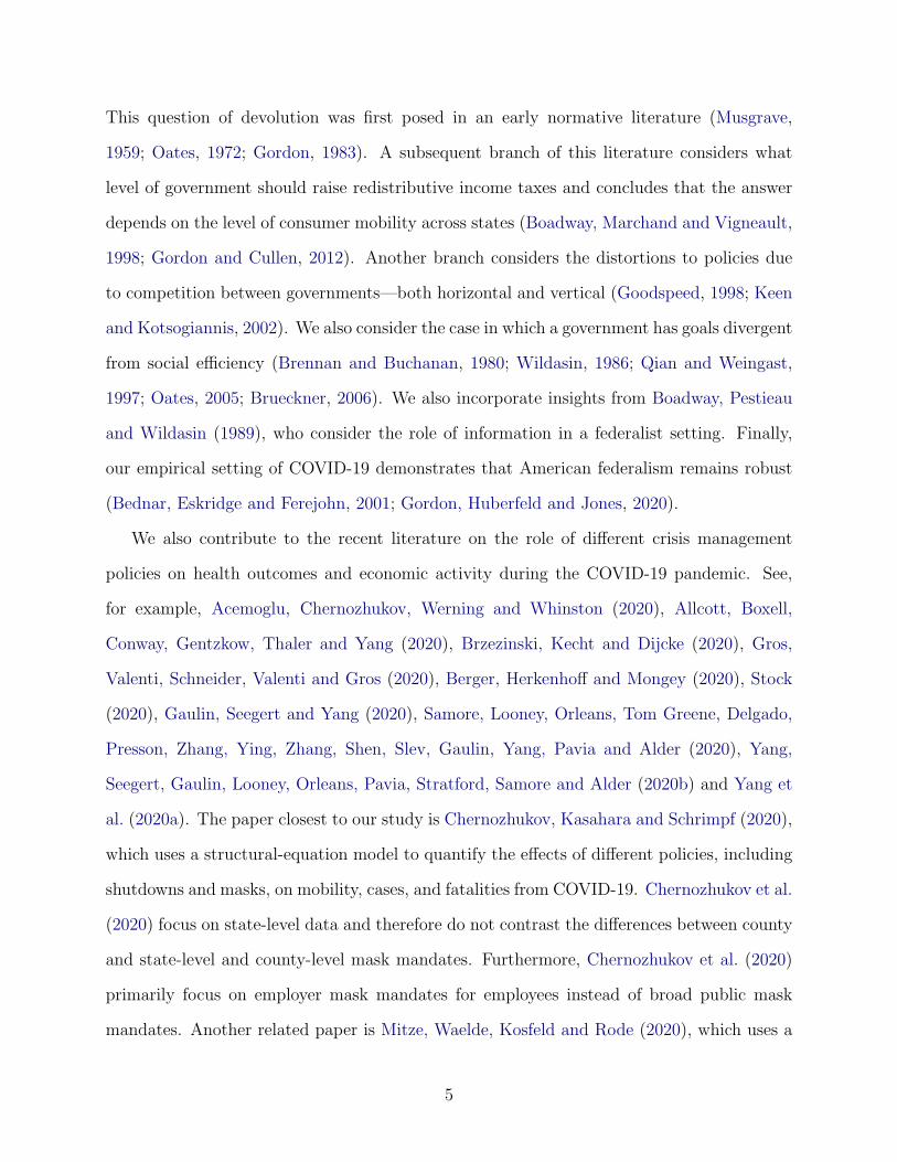
This question of devolution was first posed in an early normative literature (Musgrave,

1959; Oates, 1972; Gordon, 1983). A subsequent branch of this literature considers what

level of government should raise redistributive income taxes and concludes that the answer

depends on the level of consumer mobility across states (Boadway, Marchand and Vigneault,

1998; Gordon and Cullen, 2012). Another branch considers the distortions to policies due

to competition between governments—both horizontal and vertical (Goodspeed, 1998; Keen

and Kotsogiannis, 2002). We also consider the case in which a government has goals divergent

from social efficiency (Brennan and Buchanan, 1980; Wildasin, 1986; Qian and Weingast,

1997; Oates, 2005; Brueckner, 2006). We also incorporate insights from Boadway, Pestieau

and Wildasin (1989), who consider the role of information in a federalist setting. Finally,

our empirical setting of COVID-19 demonstrates that American federalism remains robust

(Bednar, Eskridge and Ferejohn, 2001; Gordon, Huberfeld and Jones, 2020).

We also contribute to the recent literature on the role of different crisis management

policies on health outcomes and economic activity during the COVID-19 pandemic. See,

for example, Acemoglu, Chernozhukov, Werning and Whinston (2020), Allcott, Boxell,

Conway, Gentzkow, Thaler and Yang (2020), Brzezinski, Kecht and Dijcke (2020), Gros,

Valenti, Schneider, Valenti and Gros (2020), Berger, Herkenhoff and Mongey (2020), Stock

(2020), Gaulin, Seegert and Yang (2020), Samore, Looney, Orleans, Tom Greene, Delgado,

Presson, Zhang, Ying, Zhang, Shen, Slev, Gaulin, Yang, Pavia and Alder (2020), Yang,

Seegert, Gaulin, Looney, Orleans, Pavia, Stratford, Samore and Alder (2020b) and Yang et

al. (2020a). The paper closest to our study is Chernozhukov, Kasahara and Schrimpf (2020),

which uses a structural-equation model to quantify the effects of different policies, including

shutdowns and masks, on mobility, cases, and fatalities from COVID-19. Chernozhukov et al.

(2020) focus on state-level data and therefore do not contrast the differences between county

and state-level and county-level mask mandates. Furthermore, Chernozhukov et al. (2020)

primarily focus on employer mask mandates for employees instead of broad public mask

mandates. Another related paper is Mitze, Waelde, Kosfeld and Rode (2020), which uses a

5

synthetic-control method to quantify the impact of mask mandates across German states.

This paper primarily focuses on changes in case growth and analyzes neither the economic

impact of mask mandates nor the question of the optimal governmental level of implemen-

tation. We add to this literature an investigation of how institutional design and delegation

of policy responsibility affect the effectiveness of policy tools in combating COVID-19 and

the related economic crisis.

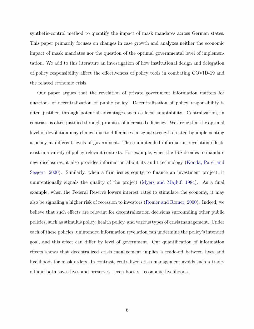
Our paper argues that the revelation of private government information matters for

questions of decentralization of public policy. Decentralization of policy responsibility is

often justified through potential advantages such as local adaptability. Centralization, in

contrast, is often justified through promises of increased efficiency. We argue that the optimal

level of devolution may change due to differences in signal strength created by implementing

a policy at different levels of government. These unintended information revelation effects

exist in a variety of policy-relevant contexts. For example, when the IRS decides to mandate

new disclosures, it also provides information about its audit technology (Konda, Patel and

Seegert, 2020). Similarly, when a firm issues equity to finance an investment project, it

unintentionally signals the quality of the project (Myers and Majluf, 1984). As a final

example, when the Federal Reserve lowers interest rates to stimulate the economy, it may

also be signaling a higher risk of recession to investors (Romer and Romer, 2000). Indeed, we

believe that such effects are relevant for decentralization decisions surrounding other public

policies, such as stimulus policy, health policy, and various types of crisis management. Under

each of these policies, unintended information revelation can undermine the policy’s intended

goal, and this effect can differ by level of government. Our quantification of information

effects shows that decentralized crisis management implies a trade-off between lives and

livelihoods for mask orders. In contrast, centralized crisis management avoids such a trade-

off and both saves lives and preserves—even boosts—economic livelihoods.

6

2 Motivating Stylized Facts

The United States federal government left the determination of public safety measures in

response to the COVID-19 pandemic up to the individual states and counties throughout

2020. Riverside County, California, imposed the first mask mandate at the beginning of

April. The first state mask mandate was put in place by New York state on April 17,

and the most recent state mandate in our sample was put in place by Mississippi at the

beginning of August. From the beginning of April to the beginning of August, 37 states plus

Washington D.C. enacted state-wide mask-wearing mandates. Additionally, from April to

September, 136 counties across 29 states put in place county-wide mask-wearing mandates.

This patch-work approach provides heterogeneity in the timing and the level of government

policy interventions. This heterogeneity offers a natural laboratory to study the public’s

reactions to public-safety regulations.

Table 1 presents the summary statistics for our sample period. The sample period spans

the 90 days before and after a state- or county-level mask mandate was put in place (offset

by one week before the mask mandate to account for announcement effects). Our primary

proxies of economic activity are consumer mobility,2 which measures the amount of traffic

at economically relevant activities (e.g., retail shopping and transportation) as a percentage

of the prior year’s activity levels, and consumer spending from Facteus, with which we

calculate average spending per person per month.3 Over the sample period (90 days before

and after a mask mandate), the average mobility is 14% lower than for the equivalent period

2Our mobility proxy comes from Google’s cellphone-location based mobility data, a daily-frequency com-parison of mobility relative to the same calendar day in the prior year; for more detail see Yang et al.(2020a).

3The Facteus data contains credit card spending data from multiple payment processing companies butonly covers a subset of processed spending. This data provides spending based on residence and, unfor-tunately, does not distinguish between online versus in-person spending. To derive an economically inter-pretable coefficient of ”spending per person per month,” we calculate the full-sample average number oftransactions from Facteus per population, which is 0.04 daily transactions per person, or, assuming roughlyone credit card transaction per person per day (a conservative estimate), the Facteus data comprises 1/0.04or 1/25 of daily spending or 1/(30 * 25) of monthly spending. However, we have no reason to believe thereare selection issues in this consumer spending proxy. To arrive at our final proxy for spending / month, wemultiply our spending per person by 30 * 25.

7

in 2019, reflecting the general reduction in economic activity observed throughout much of

2020 (Yang et al., 2020a). However, the average mobility around county-level mandates is

23% lower than the equivalent period in 2019. Similarly, spending per month is lower in the

county-level mandate sample.

The information conveyed by the news of a mandate might differ depending on whether it

comes from the county or the state. For example, the daily new infection rate in states around

the mandates was 10 per 100,000 residents, while the equivalent number around county

mandates was 15. This evidence suggests that the difference in information revealed may be

partially due to true differences in new cases. The increased rate for county mandates is also

reflected in the variable High county, which shows that 78% of the county mandates have

above-median event-day-0 infection rates, compared to only 49% for state-level mandates.

This evidence is consistent with the idea that county mandates were put in place in response

to heightened infection rates and depressed economic activity in that county, whereas state

mandates, which affect a larger region, may not reflect such acute statistics.

The counties enacting mandates are more urban (Urban county is 76% compared to 23%

for state mandates) and adopt those mandates earlier in time (Early county is 66% com-

pared to 55% for state mandates). According to survey data published by The New York

Times (Comply county), 87% of residents covered by a county mandate reported compliance

with a mask mandate, a figure substantially higher than the 67% under state mandates.

Lastly, the counties enacting mask mandates are slightly more liberal, with only 43% being

majority conservative. However, 82% counties under state mandates are conservative (Red

county, based on 2016 presidential vote). Similarly, 77% of the counties with county man-

dates occurred in conservative states, and 65% of counties with state mandates occurred in

conservative states. Liberal counties also adopted mandates earlier than their conservative

counterparts, as we see in Table A.1, which shows a –0.2 correlation coefficient between Early

county and Red county. In Figure 1, we show the geographic dispersion of counties and states

with mask mandates. There is significant overlap between county-level mask mandates and

8

state-level mask mandates. In these cases, we consider the order which was put in place

earlier (e.g., Riverside County, California).

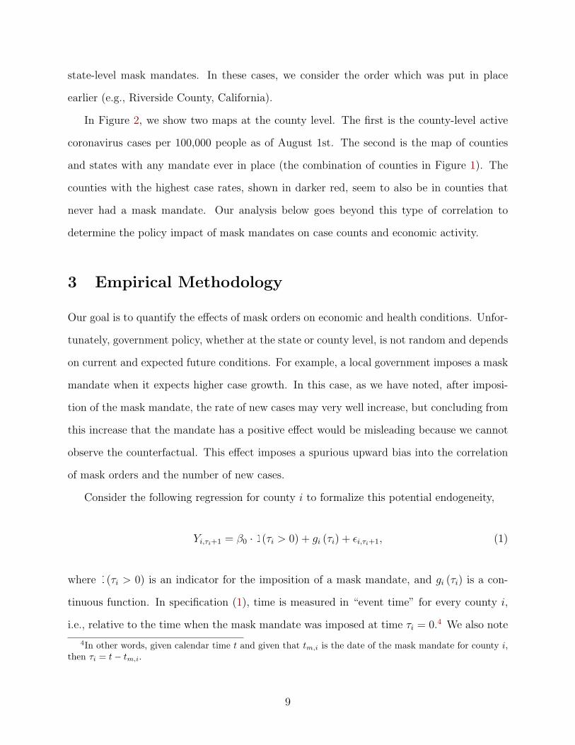
In Figure 2, we show two maps at the county level. The first is the county-level active

coronavirus cases per 100,000 people as of August 1st. The second is the map of counties

and states with any mandate ever in place (the combination of counties in Figure 1). The

counties with the highest case rates, shown in darker red, seem to also be in counties that

never had a mask mandate. Our analysis below goes beyond this type of correlation to

determine the policy impact of mask mandates on case counts and economic activity.

3 Empirical Methodology

Our goal is to quantify the effects of mask orders on economic and health conditions. Unfor-

tunately, government policy, whether at the state or county level, is not random and depends

on current and expected future conditions. For example, a local government imposes a mask

mandate when it expects higher case growth. In this case, as we have noted, after imposi-

tion of the mask mandate, the rate of new cases may very well increase, but concluding from

this increase that the mandate has a positive effect would be misleading because we cannot

observe the counterfactual. This effect imposes a spurious upward bias into the correlation

of mask orders and the number of new cases.

Consider the following regression for county i to formalize this potential endogeneity,

Yi,τi+1 = β0 · 1(τi > 0) + gi (τi) + εi,τi+1, (1)

where 1(τi > 0) is an indicator for the imposition of a mask mandate, and gi (τi) is a con-

tinuous function. In specification (1), time is measured in “event time” for every county i,

i.e., relative to the time when the mask mandate was imposed at time τi = 0.4 We also note

4In other words, given calendar time t and given that tm,i is the date of the mask mandate for county i,then τi = t− tm,i.

9

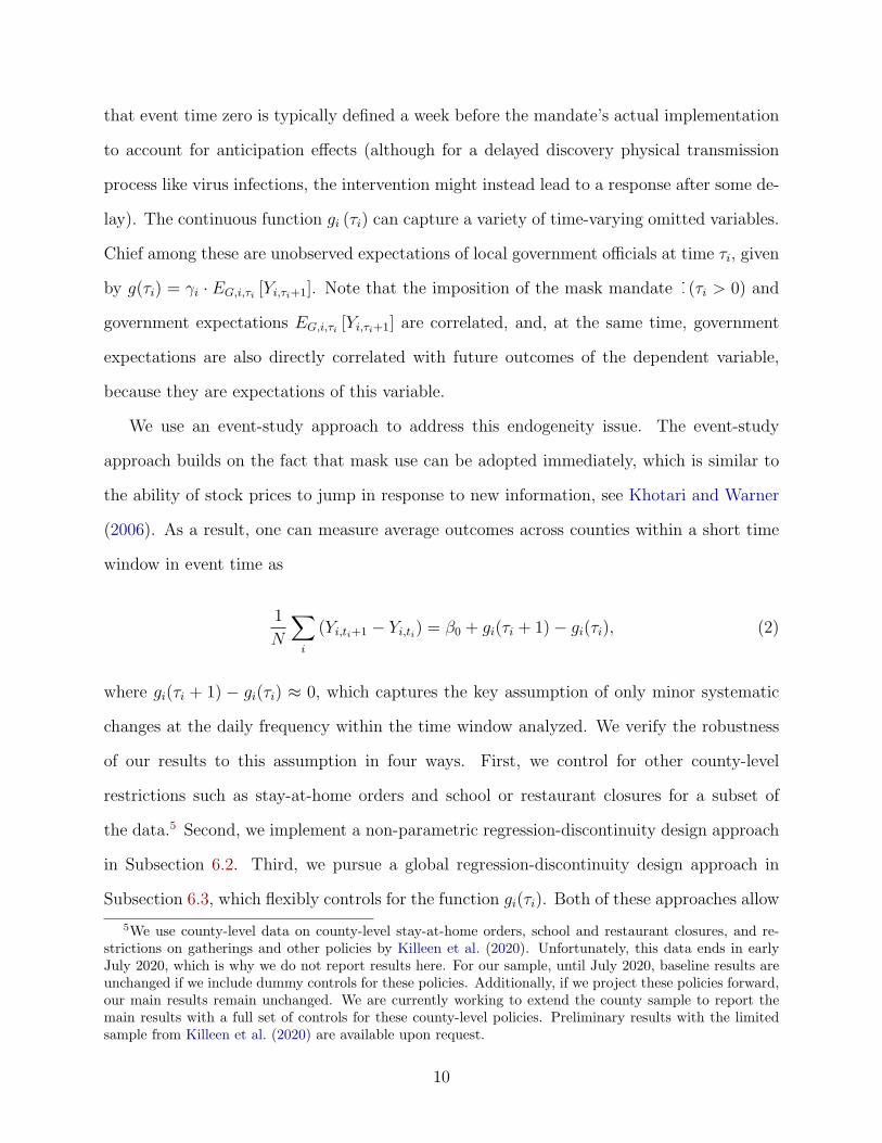
that event time zero is typically defined a week before the mandate’s actual implementation

to account for anticipation effects (although for a delayed discovery physical transmission

process like virus infections, the intervention might instead lead to a response after some de-

lay). The continuous function gi (τi) can capture a variety of time-varying omitted variables.

Chief among these are unobserved expectations of local government officials at time τi, given

by g(τi) = γi · EG,i,τi [Yi,τi+1]. Note that the imposition of the mask mandate 1(τi > 0) and

government expectations EG,i,τi [Yi,τi+1] are correlated, and, at the same time, government

expectations are also directly correlated with future outcomes of the dependent variable,

because they are expectations of this variable.

We use an event-study approach to address this endogeneity issue. The event-study

approach builds on the fact that mask use can be adopted immediately, which is similar to

the ability of stock prices to jump in response to new information, see Khotari and Warner

(2006). As a result, one can measure average outcomes across counties within a short time

window in event time as

1

N

∑i

(Yi,ti+1 − Yi,ti) = β0 + gi(τi + 1)− gi(τi), (2)

where gi(τi + 1) − gi(τi) ≈ 0, which captures the key assumption of only minor systematic

changes at the daily frequency within the time window analyzed. We verify the robustness

of our results to this assumption in four ways. First, we control for other county-level

restrictions such as stay-at-home orders and school or restaurant closures for a subset of

the data.5 Second, we implement a non-parametric regression-discontinuity design approach

in Subsection 6.2. Third, we pursue a global regression-discontinuity design approach in

Subsection 6.3, which flexibly controls for the function gi(τi). Both of these approaches allow

5We use county-level data on county-level stay-at-home orders, school and restaurant closures, and re-strictions on gatherings and other policies by Killeen et al. (2020). Unfortunately, this data ends in earlyJuly 2020, which is why we do not report results here. For our sample, until July 2020, baseline results areunchanged if we include dummy controls for these policies. Additionally, if we project these policies forward,our main results remain unchanged. We are currently working to extend the county sample to report themain results with a full set of controls for these county-level policies. Preliminary results with the limitedsample from Killeen et al. (2020) are available upon request.

10

us to control for continuous, time-varying unobservables in event-time, which correspond to

gi(τi). Finally, in Subsections 6.2 and 6.2, we report estimates from placebo tests using

variation in location and time.

4 Empirical Evidence

In this section, we study the effects of a mask mandate and how they vary when a state

or a county establishes the order. We report three different measures at the county level.

Mobility, the change in consumer activity with respect to the same day last year, Cases/pop,

the daily new cases per 100,000 population, and Spend/month, daily credit card spending

per person (scaled to the monthly level for economic interpretation).

A county mandate likely provides more information about contagion risk to people be-

cause the county’s case rates probably drive the government decision. In contrast, the

decision to enact a state-wide mandate weighs information from the entire state. As such,

it provides an attenuated signal about the contagion risk in any given county. Therefore,

we expect to observe a stronger information signal from enacting county mandates than

state mandates, leading individuals to update their beliefs about contagion rates more so

for county mandates. As a result, we expect this signal to reduce or even overwhelm the

mask-mandate’s direct effect to minimize risk and increase economic activity.

When the mask mandates’ direct effect is larger than the information channel, we expect

mobility and spending to increase because these activities have now become safer. When

enacting a mandate is accompanied by a larger information shock, we expect increased

mobility and spending to be attenuated and potentially decrease. We expect cases to fall

after a mandate; the extent, however, may differ by level of government due to enforcement.

In Table 2 and Figure 3, we report estimates of how the three dependent variables change

over the 25 days before and after a county or state mandate. We measure mobility and

spending one week before the mask mandate to account for leakage of information. We

11

measure the new case rates ten days after to account for testing delays (of three to four days

on average) and symptom onset (of two to fourteen days).6 Our findings are not sensitive to

this timing. We report estimates with different timing and time polynomials to account for

potential information leakage and mechanical testing lags as an alternative. The sample in

the first three columns comprises all counties in a state with a state mandate that did not

already have a county mandate. The sample in the last three columns comprises counties

that enacted a county mandate (when no state mandate was already in place). We include

county-fixed effects, as well as calendar-day-fixed effects.

From Table 2, we find that when a mask mandate is ordered by the state, mobility and

spending increase by 2.7% and 2.0% of their means, respectively, which is consistent with

the direct effect being stronger than the information effect. Specifically, in columns (1) and

(3), we report that mobility increases by 0.39 percentage points and spending increases by

$23.89 per person per month, respectively. This evidence suggests that people believe that

they face less risk when engaging in economic activity with the mask mandate in place.

Simply put, they go out and consume more. Meanwhile, cases per population decrease,

despite the increased mobility. In Figure 3, we show that after the mandate, new cases

appear to stop increasing entirely, suggesting that the mask mandate reduces the spread of

the disease. Together, this evidence suggests that state-wide mask mandates achieve their

economic and health goals.

As expected, the information channel appears to be stronger for county-level mask man-

dates. After a county enacts a mask mandate, we observe a decrease in mobility of 0.51

percentage points or 2.2% relative to the mean. This reaction is consistent with people

updating their risk assessment of COVID-19 and partially or fully quarantining. Spending

does not increase as it does under the state mandate, and Figure 3 shows that the downward

trend in spending continues relatively unaffected. The number of new cases per 100,000

people decreases substantially after the mandate; column (5) reports that cases decreased by

6See 50-State COVID-19 project covidstates.org and CDC cdc.gov/coronavirus/2019-ncov/symptoms-testing/symptoms.html.

12

two people per 100,000, a 13% decrease relative to the mean. Consistent with this finding, in

Figure 3, we show a significant decrease in the growth of new cases. This strong public health

impact likely combines the effect of increased mask-wearing and the substantial decrease in

mobility observed after county mask orders.

In sum, we find that, although county-level mask mandates may seek to decrease health

risks and potentially benefit consumer confidence, they also provide a strong signal that

increases consumers’ perceived risk of contracting COVID-19. When this indirect channel is

significant enough, as observed in county mandates, the information effect dominates, and

the net impact on economic activity is negative.

5 Treatment Effect Heterogeneity

This section considers heterogeneous responses across several dimensions that affect the

response to mask mandates. For example, prior beliefs about COVID-19 contagion risk

likely depended on information people received before the mask mandate. The information

people receive, in turn, is partially influenced by news consumption habits (e.g., conservative

or liberal sources). People’s prior beliefs were also likely affected by whether the cases were

initially high or low and whether the mandate came early in the pandemic or later. Similarly,

people’s priors are likely affected by externalities from other people’s choices, which varies

based on the local population density.

While we present one interaction effect at a time here, we show in Appendix B that our

results are broadly unchanged if we jointly analyze all interaction effects together.

5.1 Differences by political affiliation counties

In Table 3, we report the effect of state and county mask orders on mobility, case growth

per population, and spending per person, interacted with an indicator variable for conser-

13

vative counties.7 We denote conservative counties as red for short. We designate a county

as conservative if it recorded more votes for the Republican presidential candidate in 2016

than the Democratic one, and liberal otherwise. The estimates are similar for other polit-

ical affiliation measures, including vote shares in different elections and google searches for

partisan phrases such as “plandemic.”

We find that mobility increases after a state-enforced mask order, but substantially less

so in conservative counties. Specifically, in column (1), we report that the coefficient on the

interaction between state mask mandate and conservative county is roughly -0.40, and the

coefficient on state mask mandate is about 0.71, both relatively precisely estimated. This

evidence suggests that mobility increases following a state mandate but less so in conservative

counties than liberal ones. This result is consistent with the presence of an information effect

in state mandates, albeit weaker than the information effect in the county mask mandates.

In other words, this evidence is consistent with conservatives, who previously believed the

risks from COVID-19 were low, after the mask mandate believing the risk is high—leading

them to go out and spend less, while liberals, who previously thought the risks were high,

now start going out and spending with a new confidence that comes with the mandate.8 For

county mask mandates, column (4) shows that this information effect is strongly driven by

red counties and is strong enough to reduce mobility. Column (4) also shows that liberal

counties see a slight increase in mobility in response to county mask mandates, though this

is imprecisely estimated. These findings suggest that people in liberal counties either had

a higher prior risk assessment or did not view the county-level mask mandate as providing

much new information about local infection risks.

Confirmed cases decrease substantially less in conservative counties in the days imme-

diately following state-level mask mandates, which we report in column (2) of Table 3.

Specifically, the coefficient on state mask is -2.58, and the coefficient on the interaction be-

7We also report figures for non-parametric regression-discontinuity design estimates in Figure A.1.8We consider this a reasonable assumption. For example, at a Trump campaign rally in February, Presi-

dent Trump said, “Now the Democrats are politicizing the coronavirus ... This is their new hoax.”

14

tween state mask and conservative county is 2.07, both estimated relatively precisely. One

possible explanation for this pattern is that people in conservative counties respond to state

mandates less and are therefore more mobile and continue to get infected.

There is no discernible difference in spending per person in conservative and liberal

counties following a mask mandate. In columns (3) and (6) of Table 3, we report that

spending increases following a state mask order but does not following a county order. The

interaction effect for conservative counties, while typically positive, is small economically

and statistically insignificant.

We provide additional estimates of political affiliation in appendix Table A.2. In this

table, we report estimates allowing differing responses for conservative or non-conservative

counties in conservative states or non-conservative states. We find that counties—either

liberal or conservative—in conservative states decrease their mobility more than conservative

counties, whether in conservative or liberal states. Although state mask mandates still imply

increased mobility for conservative counties in blue states, mobility responses are almost zero

for (liberal or conservative) counties in conservative states. Furthermore, Table A.2 shows

that case growth tends to fall less in conservative states and conservative counties. This

evidence is consistent with conservative states having a greater threshold to enforce a mask

mandate and, therefore, a larger information revelation effect when the mandate is enforced.

5.2 Differences across urban and rural counties

In Table 4, we report the effect of mask mandates separately for urban and rural counties9.

We designate a county as urban if more than 50% of its population lives in an urban area,

and rural otherwise. The externality created by going out to stores or restaurants without a

mask is greater in urban areas than rural because contagion risk increases with population

density. As a result of this relative difference in the direct effect, we expect that mask

mandates will increase mobility and spending and decrease case rates more in urban areas

9We also report results from non-parametric regression-discontinuity design estimates in figure A.2

15

than in rural areas.

The evidence across urban and rural counties is consistent with our predictions of dif-

ferences in the direct channel. In Column (1) of Table 4, we report that mobility increases

less in urban counties following a state mask mandate as shown by the coefficient −0.295.

This evidence is consistent with the view that infection risk is generally higher in denser

areas, which implies that people will be more hesitant to be mobile, even if other people

wear masks.

Following county-level mask mandates, mobility decreases more in urban counties. Re-

garding case growth, we find that both state and county mask mandates effectively dampen

COVID-19 spread. It should be noted that urban counties see a consistent reduction in case

growth by about 2.7 cases per 100K, while case growth reduction from state mask mandates

is somewhat less effective for rural counties.

Consistent with our mobility estimates, we also document in Table 4 that urban counties

see a strong increase in credit card spending in response to state mask mandates. In contrast,

they see a slight decrease by around $8 per month ($26.58− $35.52).

5.3 Differences across counties with high and low number of cases

A mask mandate might reveal especially high levels of infection risk in counties with a high

initial level of case counts. This prediction follows from the pitfalls of monitoring infection

risks of contagious diseases with exponential growth dynamics. Initially, case numbers are

very low, and the risks of exponential growth in infectious people are underestimated. How-

ever, with higher base rates, the same exponential growth rate implies a non-linear increase

in the number of newly infected people. This non-linear dynamic can result in sudden shifts

in risk assessment, as risks are deemed negligible in the initial weeks but then appear sud-

denly very imminent as the number of new cases rises higher. Therefore, a given infection

growth rate might signal disproportionately higher infection risk if the currently known base

rate of cases is high.

16

Consistent with our predictions, we find that mobility increases in response to state mask

mandates are very muted in counties with a high number of cases. Specifically, in Columns

(1) and (4) of Table 5, we report that the interaction between high case county and state mask

mandate (in Column 1) and high case county and county mask mandate (in Column 4) are

negative, large, and relatively precisely estimated.10 In the case of county mask mandates,

the effect on mobility in high case counties is large enough to reduce overall mobility. The

negative interaction effects are consistent with the view that mask mandates in general signal

particularly high risks in counties with high initial levels of confirmed COVID-19 cases.

Columns (2) and (5) of Table 5 show that both state and county mask mandates are

effective in dampening case growth, especially for counties with a high initial level of cases.

The evidence on spending is more mixed. While state mandates stimulate credit card spend-

ing, they do so actually more in high case counties. The effect of state mask mandates in

high case counties is almost double the effect with an increase by $31.23 = ($16.25 + $14.98)

per month and person. In contrast, there is no significant effect of county mask mandates

on credit card spending.

5.4 Differences across counties with earlier or later mandates

COVID-19 initially arrived in major global cities, such as the New York metropolitan area,

the San Francisco Bay area, and Seattle-Tacoma metropolitan area. As a result of the

disease’s early geographic concentration, locations that imposed mask mandates early reveal

much more information on infection risk. In contrast, by fall 2020, COVID-19 had spread

from the coastal areas of the U.S. to almost all counties and had penetrated rural and even

remote areas. Consequently, later adoption of mask mandates is likely to have revealed

less information about infection risks, both because more time had passed and because the

disease was more widespread.

If this is the case, then mobility in early counties with county-level mandates will decrease

10We also report results from non-parametric regression-discontinuity design estimates in Figure A.3.

17

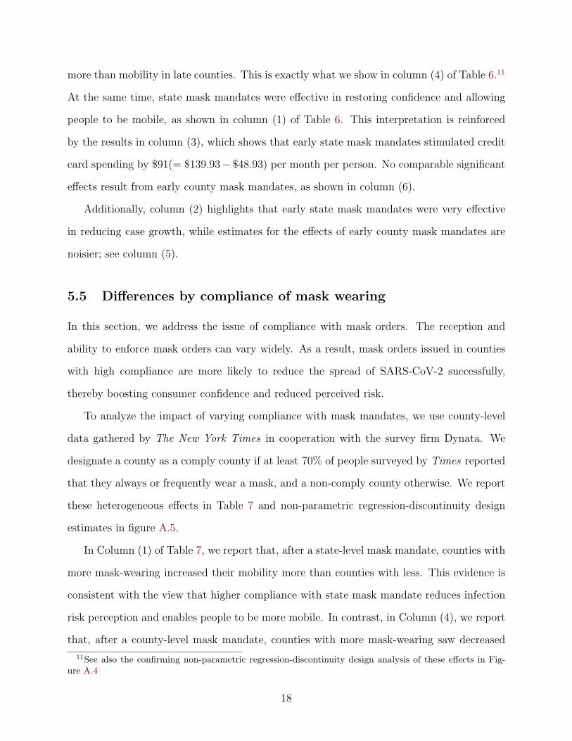
more than mobility in late counties. This is exactly what we show in column (4) of Table 6.11

At the same time, state mask mandates were effective in restoring confidence and allowing

people to be mobile, as shown in column (1) of Table 6. This interpretation is reinforced

by the results in column (3), which shows that early state mask mandates stimulated credit

card spending by $91(= $139.93− $48.93) per month per person. No comparable significant

effects result from early county mask mandates, as shown in column (6).

Additionally, column (2) highlights that early state mask mandates were very effective

in reducing case growth, while estimates for the effects of early county mask mandates are

noisier; see column (5).

5.5 Differences by compliance of mask wearing

In this section, we address the issue of compliance with mask orders. The reception and

ability to enforce mask orders can vary widely. As a result, mask orders issued in counties

with high compliance are more likely to reduce the spread of SARS-CoV-2 successfully,

thereby boosting consumer confidence and reduced perceived risk.

To analyze the impact of varying compliance with mask mandates, we use county-level

data gathered by The New York Times in cooperation with the survey firm Dynata. We

designate a county as a comply county if at least 70% of people surveyed by Times reported

that they always or frequently wear a mask, and a non-comply county otherwise. We report

these heterogeneous effects in Table 7 and non-parametric regression-discontinuity design

estimates in figure A.5.

In Column (1) of Table 7, we report that, after a state-level mask mandate, counties with

more mask-wearing increased their mobility more than counties with less. This evidence is

consistent with the view that higher compliance with state mask mandate reduces infection

risk perception and enables people to be more mobile. In contrast, in Column (4), we report

that, after a county-level mask mandate, counties with more mask-wearing saw decreased

11See also the confirming non-parametric regression-discontinuity design analysis of these effects in Fig-ure A.4

18

mobility relative to counties with less mask-wearing. This result potentially stems from

people in counties with higher mask-wearing compliance being more risk-averse to the virus.

For both state and county mask mandates, we find that case growth is significantly

reduced for high mask-wearing compliance counties. Interestingly the reduction in case

growth is even larger for county mask mandates than state mask mandates. This result is

consistent with high compliance people being more risk-averse to infection risks.

6 Sensitivity of estimates

This section considers additional specifications and placebo tests to explore potential threats

to identification. To identify the effects of mask orders, the estimates presented previously

have relied on the staggered implementation of mask orders and the smoothness of potential

confounding factors around the time of implementation.

Our identification strategy relied on two key features. First, mask mandate policies

vary both across time and across counties. Second, our event-study approach relied on the

assumption that continuous unobservable effects are negligible within our short-run time

windows.

This section stress tests these two features in reverse order. First, we address the potential

impact of continuous unobservables on our event-study design. We extend these estimates

by considering a (non-parametric and parametric) regression-discontinuity design.

Second, we provide two placebo tests to ensure that the mask mandate variation drives

our results and not unobserved features of either the time or the treatment counties we

analyze.

First, we provide a location placebo created by assigning treatment status to counties

that did not enact mandates but are adjacent to counties that did. The placebo treatment

assignment is chosen at the same time as the treatment assignment of the counties with

mask mandates. This location placebo allows us to verify that our effects are not driven by

19

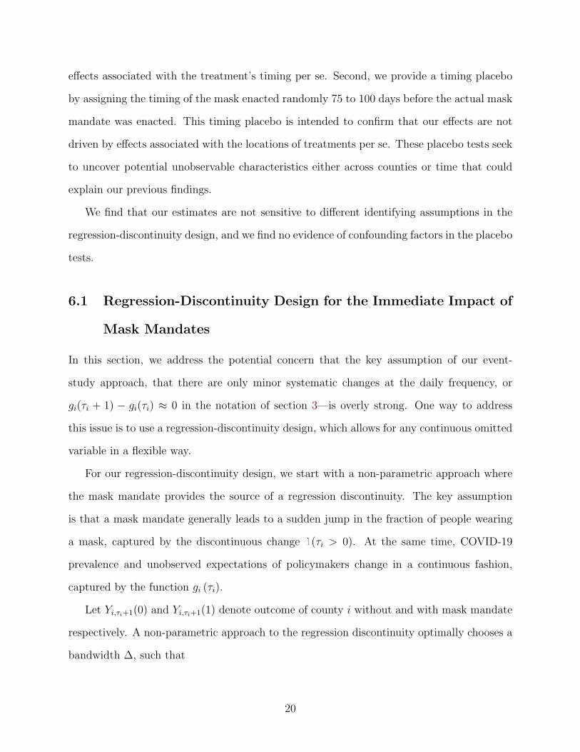
effects associated with the treatment’s timing per se. Second, we provide a timing placebo

by assigning the timing of the mask enacted randomly 75 to 100 days before the actual mask

mandate was enacted. This timing placebo is intended to confirm that our effects are not

driven by effects associated with the locations of treatments per se. These placebo tests seek

to uncover potential unobservable characteristics either across counties or time that could

explain our previous findings.

We find that our estimates are not sensitive to different identifying assumptions in the

regression-discontinuity design, and we find no evidence of confounding factors in the placebo

tests.

6.1 Regression-Discontinuity Design for the Immediate Impact of

Mask Mandates

In this section, we address the potential concern that the key assumption of our event-

study approach, that there are only minor systematic changes at the daily frequency, or

gi(τi + 1) − gi(τi) ≈ 0 in the notation of section 3—is overly strong. One way to address

this issue is to use a regression-discontinuity design, which allows for any continuous omitted

variable in a flexible way.

For our regression-discontinuity design, we start with a non-parametric approach where

the mask mandate provides the source of a regression discontinuity. The key assumption

is that a mask mandate generally leads to a sudden jump in the fraction of people wearing

a mask, captured by the discontinuous change 1(τi > 0). At the same time, COVID-19

prevalence and unobserved expectations of policymakers change in a continuous fashion,

captured by the function gi (τi).

Let Yi,τi+1(0) and Yi,τi+1(1) denote outcome of county i without and with mask mandate

respectively. A non-parametric approach to the regression discontinuity optimally chooses a

bandwidth ∆, such that

20

E[Yi,τi+1

∣∣−∆ < τi < 0]≈E

[Yi,τi+1(0)

∣∣τi = 0]

E[Yi,τi+1

∣∣0 ≤ τi < ∆]≈E

[Yi,τi+1(1)

∣∣τi = 0],

(3)

where, as we will show in the estimation section ∆ is typically 25 days, using optimal band-

width selection methods such as Imbens and Kalyanaraman (2011) and Calonico, Cattaneo

and Titinuik (2014). The jump in outcome Yi,τi+1 at τi = 0, therefore, identifies the imme-

diate mask impact

β0 = E[Yi,τi+1(1)

∣∣τi = 0]− E

[Yi,τi+1(0)

∣∣τi = 0]. (4)

We also consider parametric versions of specification in equation (1), by using flexible

polynomial functions to control for gi (τi). This specification is especially useful for analyzing

interaction effects because it allows us to report comparable estimates across specifications

while also allowing us to control for location- and time-fixed effects.

Being aware of recent criticisms of using regression-discontinuity designs with time as

a forcing variable, such as in Hausman and Rapson (2018), we caution the reader not to

overweight the importance of these estimates relative to our main results. However, we also

note that our setting is different from many of the setups discussed in Hausman and Rapson

(2018) in at least two respects.

First, Hausman and Rapson (2018) focus on settings without cross-sectional variation,

where estimation bandwidths are often extended to increase power. In contrast, we have

rich cross-sectional variation, such that we can rely on cross-sectional asymptotics instead of

time-series asymptotics as criticized by Hausman and Rapson (2018). Second, Hausman and

Rapson (2018) caution that dependent variables might exhibit persistence. We maintain that

this is less of an issue for our economic variables, especially mobility and spending because

these are flow variables that can adjust almost immediately. Additionally, we use changes in

case growth precisely to reduce the influence of persistence in this data.

21

Table 8 reports the result of the non-parametric regression-discontinuity design in event

time. Almost all of our main results are qualitatively similar in this specification, confirming

that our event-study approach is not systematically biased. We note that the economic

effects are generally larger in magnitude in the non-parametric regression-discontinuity design

specification, while the county mask mandate effects tend to be noisier than in our baseline

event study result recorded in Table 2.

Table 9 reports additional parametric regression-discontinuity design estimates using ei-

ther first- or third-order polynomials to control for continuous unobservables in event time.

Encouragingly, these results are quantitatively very close to our main results in Table 2 for

linear event-time controls and somewhat stronger for third-order polynomials.

Overall, the assumption that continuous unobservables only have a small impact on

outcomes is reasonably robust.

6.2 Location Placebo Tests

Placebo tests provide a check on the likelihood that unobservable characteristics could drive

the results. If our specifications measure the true effect of mask mandates, we should find no

impact if we assign treatment to counties that did not enact a mask mandate and rerun our

specifications. We select all counties without a county or state mandate that are adjacent

to a county that enacts one (or is in a state that enacts one). Initially, 2,188 counties have

a county or state mandate, and with this designation, we have 370 placebo counties. We

assign the time of the mask mandate for these placebo counties to be the adjacent county’s

time, and if there are multiple adjacent counties with mask mandates, we take the average

time.

In Table 10, we report these placebo tests for both our event-study design (in equation (2))

and regression-discontinuity design (in equation (4)). In panel A, we find no statistically sig-

nificant effects on mobility, cases per 100,000 people, or spending per person per month with

state or county mask mandates. In panel B, we similarly find no evidence of a discontinuity

22

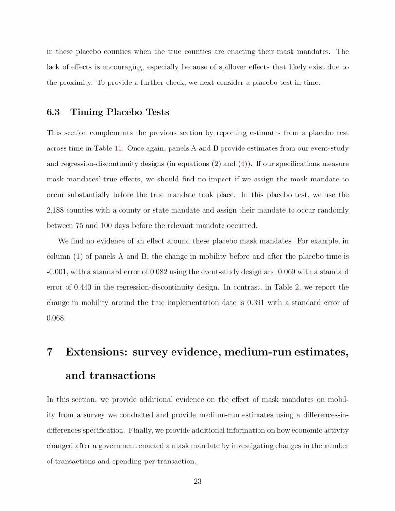
in these placebo counties when the true counties are enacting their mask mandates. The

lack of effects is encouraging, especially because of spillover effects that likely exist due to

the proximity. To provide a further check, we next consider a placebo test in time.

6.3 Timing Placebo Tests

This section complements the previous section by reporting estimates from a placebo test

across time in Table 11. Once again, panels A and B provide estimates from our event-study

and regression-discontinuity designs (in equations (2) and (4)). If our specifications measure

mask mandates’ true effects, we should find no impact if we assign the mask mandate to

occur substantially before the true mandate took place. In this placebo test, we use the

2,188 counties with a county or state mandate and assign their mandate to occur randomly

between 75 and 100 days before the relevant mandate occurred.

We find no evidence of an effect around these placebo mask mandates. For example, in

column (1) of panels A and B, the change in mobility before and after the placebo time is

-0.001, with a standard error of 0.082 using the event-study design and 0.069 with a standard

error of 0.440 in the regression-discontinuity design. In contrast, in Table 2, we report the

change in mobility around the true implementation date is 0.391 with a standard error of

0.068.

7 Extensions: survey evidence, medium-run estimates,

and transactions

In this section, we provide additional evidence on the effect of mask mandates on mobil-

ity from a survey we conducted and provide medium-run estimates using a differences-in-

differences specification. Finally, we provide additional information on how economic activity

changed after a government enacted a mask mandate by investigating changes in the number

of transactions and spending per transaction.

23

7.1 Survey Evidence

In this section, we report evidence from the October and November 2020 Utah Consumer

Sentiment Survey. The survey samples 400 Utah residents a month and is designed to be

similar to the Michigan Surveys of Consumers, which includes 500 completed interviews

per month. For the questions we are interested in, the sample was recruited by sending

participants a letter and paying participants $10. The sample is the universe of addresses in

Utah and sampled based on prior nonresponse rates that provide a final sample representative

of Utah (Samore et al., 2020; Yang et al., 2020b). This sampling has been shown to have

minimal nonresponse sample selection Gaulin et al. (2020). In appendix Appendix A, we

provide more details on recruitment, nonresponse, and sample balance.

In Table 12, we report responses to the question “How much more or less likely (as a

percent) would you be to go out to a store if ...” with the following seven scenarios: “The

number of confirmed cases fell by 10%,” “The number of confirmed cases fell by 50%,” “The

number of confirmed cases fell by 90%,” “Half of the people were wearing a mask,” “Everyone

was wearing a mask,” “The store enforced wearing a mask,” “The state enforced wearing a

mask.” This question is meant to determine how responsive people are to the perceived risks

associated with COVID-19.

Overall, participants report that they are very responsive to the number of confirmed

cases and how many people are wearing a mask in their locality. In response to a drop

in confirmed cases of 10%, 50%, and 90%, participants report they would increase their

likelihood of going to a store by 13%, 30%, and 57%, respectively. These correspond to elas-

ticities between 0.6 and 1.3. Similarly, respondents report that they would be substantially

more likely to go out to a store if everyone was wearing a mask (51% more likely), the store

enforced wearing a mask (50% more likely), and the state enforced wearing a mask (49%

more likely). Despite participants recognizing that a state mask mandate would not ensure

compliance, a state enforced mask mandate substantially increases their willingness to go

out to a store.

24

These survey responses suggest that mask mandates increase mobility. Mobility decreased

sharply in response to COVID-19. As a result, spending has decreased and shifted from local

services toward goods that can be shipped to one’s door. These survey responses suggest

that people believe the risk of going out to a store is substantially less if people are wearing

masks—and, as a result, increases their likelihood of going out to a store.

These survey responses also suggest the potential for a large information effect. Par-

ticipants report that they are very responsive to the COVID-19 environment. Therefore,

if mask mandates also update their beliefs of this environment, they may reduce mobility.

This highlights the importance of government messaging of policy initiatives.

7.2 Medium-run estimates

To extend our analysis to the medium-run, we rely on synthetic control methods developed

by Abadie, Diamond and Hainmueller (2010, 2015) and Abadie and Gardeazabal (2003).

The basic identification challenge we face is that expectations of local government officials

are unobservable, as discussed in Section 3. However, as we increase the time horizon T

for estimation, the assumption that changes in continuous omitted variables are negligible

gi(τi + T )− gi(τi) ≈ 0, becomes clearly untenable. Instead, synthetic control methods allow

us to flexibly control for time-varying functions gi(τi + T ), which capture variables such as

unobserved expectations of local government officials.

We construct synthetic control counties to control for time-varying unobservable charac-

teristics. Specifically, we construct control counties by weighting counties that do not have

a county or state mask mandate to match counties with a state or county mandate

Yi,τi+1 =N∑j=1

wj · Yj,τi+1 (5)

where j indexes counties without mask mandates. Weights wj are chosen to match pre-

treatment characteristics of county i, which eventually imposes a mask mandate. For weights

25

wj, we employ entropy weights as proposed by Hainmueller (2012). We generate these

weights matching the mean on county population, mobility, change in cases, and spending

in a pre-period.

Given our measurement in equation (5) is successful, we measure Yi,τi+T (0) = gi(τi+T )+

εi,τi+T, so we can correctly identify

βT = E[Yi,τi+T (1)− Yi,τi+T (0)

∣∣1(τi > 0), {wj}]. (6)

In Table 13 and Figure 4, we report the medium-run effects of mask mandates on mobil-

ity, cases per 100,000 people, and spending per person per month, separately for state and

county mandates. Consistent with our short-run estimates in Table 2, we find that mobility

continues the same trend as in the short-term—increasing after state mandates but decreas-

ing following county mandates. We report as much in columns (1) and (4) of Table 13.

For state mandates, medium-run mobility responses are about 9.4% higher than short-run

increases, representing a moderate increase over the two months analyzed here. In contrast,

the decline in mobility in response to county mask mandates in column (4) of Table 13 is

four times higher in the medium run than in the short run, documented in column (4) of

Table 2.

Despite this pattern in mobility, we find, as reported in columns (2) and (5) of Table 13,

that cases per 100,000 people are substantially lower after a state enacts a mask mandate

than if a county does. The quantitative impact of state mandates is similar in the short and

medium run. In contrast, while the impact of county mandates on case growth is larger in

the short run than that of state mandates, as shown in column (5) of Table 2, in the medium

run, the case-growth effect becomes insignificant and even changes sign.

Finally, in the medium term, spending increases more after a state enacts a mask mandate

than in the short-run. As shown in column (3) of Table 13, the stimulating effect of state

mask mandates substantially increases over time. The medium-run spending effect of state

26

mask mandates is 37% higher than the short-run spending effect in column (3) of Table 2.

Therefore, the medium-run analysis reinforces the ability of state mask mandates to restrict

case growth while simultaneously stimulating the economy. As in our short-run analysis, we

fail to find similar benefits for county mask mandates.

In conclusion, state mandates achieve their main policy goals by increasing mobility

and spending while reducing virus cases. In contrast, county mandates are ineffective at

increasing economic activity and do not seem to lower case counts in the medium-run.

Additionally, in Appendix C, we show that the main medium-run results of state mask

mandates—persistent beneficial effects for public health as well as economic activity—also

emerge if we use a completely different identification strategy. In Appendix C, we deploy

a differences-in-differences approach that uses adjacent counties to treatment counties as

the control group while assigning as the event date for the control group the date of mask

mandates for treatment counties. This strategy tends to strengthen our results, a surprising

outcome given that the presence of local spillovers is likely to attenuate the effects. We

discuss this point in detail in the appendix.

We interpret these results as evidence that county mask mandates’ information revelation

effects erode the potential economic benefits as consumers revise their perceived infection

risk upward.

7.3 Number of transactions and spending per transaction

In this subsection, we briefly discuss how the number of transactions and spending per trans-

action change around implementing a mask mandate. We expect the number of transactions

to be related to economic activity. For example, transactions may increase if people are

shopping at more stores. Spending per transaction may also indicate elevated economic

activity—especially if the number of transactions increases and spending per transaction

increases.

In Figure A.6, we show the number of transactions and spending per transaction 25

27

days before and after a mask mandate. The left two panels indicate that the number of

transactions and the spending per transaction increase in response to a state mask mandate.

This evidence is consistent with our other estimates of economic activity increasing around

the state mandate. The right two panels indicate that a county mandate did not produce a

large change in the percent of transactions occurring and produced only a small increase in

spending per transaction. Again, this evidence is consistent with our conclusion that mask

mandates enacted at the county-level fail to stimulate the economy.

8 Discussion: Information Effects of Mask Mandates:

Lessons for Public Policy

Government policies result in a variety of intended and unintended effects. We have shown

how information revealed by government policies can have countervailing effects to their

intended consequences. In the context of mask orders, unintended-information effects can

attenuate or reverse the sign of the intended effect. In this section, we expand our discussion

to the consequences of unintended-information effects for the evaluation of public policy.

Consider an empirical study that analyzes the effect of policy Γ on behavior or outcome

Y , which is also influenced by unobserved beliefs of economic agents B:

Y = γ · Γ + δ ·B. (7)

If policy Γ affects beliefs B, then Cov(Γ, B) 6= 0, so that any policy evaluation that ignores

the impact of the policy on beliefs results in classical omitted variables bias:

γ = γ + δ · Cov(P,B)

V ar[P ]. (8)

For concreteness, consider the case in this paper—mask mandates. The first effect is that

mask mandates increase mobility by making mobility safer (γ > 0) and thereby boosting

28

consumer confidence. However, implementing a mask mandate can also signal risk perception

by government officials. This signal affects people’s prior beliefs of the true infection rates

(Cov(P,B) 6= 0), which will decrease mobility for higher infection rates (δ < 0).

Why does this omitted-variables bias matter if the net effect is driven by the same

government policy? It matters because the relative importance of both effects can sometimes

be understood as a consequence of which level of government deploys the policy. In our

case, a centralized policy is unlikely to reveal higher risk assessments for specific counties,

thereby implying Cov(P,B) = 0 and leading to overall economic effects being dominated

by γ > 0. On the other hand, decentralized county-level mask mandates are very likely to

reveal information about local risks, so that Cov(P,B) > 0.

9 Conclusion

This paper highlights the importance of information-revelation effects of public policy and

its impact on whether or not a policy should be decentralized. This information channel has

broad implications for devolution and immediate implications for policy decisions surround-

ing COVID-19.

We document that state mask mandates during the 2020 COVID-19 pandemic reduced

case growth and promoted economic activity, as measured by mobility and credit card spend-

ing. This evidence highlights that slowing the growth of COVID-19 cases and fostering eco-

nomic activity can be complements—not substitutes. Put differently, state mask mandates

expand the policy frontier and show there is no conflict between public health and economic

recovery.

Unfortunately, not all mask mandates are created equal. We also document that county

mask mandates during the COVID-19 pandemic, while generally successful at slowing case

growth, also depressed economic activity. The stark contrast between the effects of state

and county mask mandates should be a cautionary tale for policymakers.

29

In terms of the effectiveness of mask mandates, this paper adds to a growing consensus

that increased mask-wearing slows the growth of new cases and is a critical tool in the public

health arsenal. This paper also shows the importance of mask-wearing in terms of economic

activity. Mask mandates enforced at the state level increased consumer confidence and led

to increased economic activity. Evidence from our survey bolsters this claim. People report

that they are nearly 50% more likely to go out to a store if their state enforces a mask

mandate.

Our findings provide a new consideration in determining what level of government is most

effective at implementing different policies. An information treatment accompanies many, if

not most, policy changes. For example, when the SEC changes firms’ regulations, it sends

these firms a signal about the relative importance of different activities. Similarly, when

Congress passes a stimulus package, it signals the risk and severity of a recession.

In our context, an understanding of the information effects explains why mask mandates

imply a trade-off between lives and livelihoods on the county level and why they do not

indicate such a trade-off on the state-level. These insights, therefore, highlight how public

policy can most effectively deploy mask mandates to save lives and, at the same time,

stimulate the economy.

30

References

Abadie, Alberto, Alexis Diamond, and Jens Hainmueller, “Synthetic control meth-ods for comparative case studies: Estimating the effect of California’s tobacco controlprogram,” Journal of the American Statistical Association, 2010, 105 (490), 493–505.

Abadie, Alberto, Alexis Diamond, and Jens Hainmueller, “Comparative politicsand the synthetic control method,” American Journal of Political Science, 2015, 59 (2),495–510.

Abadie, Alberto and Javier Gardeazabal, “The economic costs of conflict: A case studyof the Basque Country,” American Economic Review, 2003, 93 (1), 113–132.

Acemoglu, D., C. Chernozhukov, I. Werning, and M. Whinston, “A Multi-RiskSIR Model with Optimally Targeted Lockdown,” NBER Working Paper, 2020.

Allcott, H., L. Boxell, J. Conway, M. Gentzkow, M. Thaler, and D. Yang, “Dif-ferences in Social Distancing During the Coronavirus Pandemic,” NBER Working Paper,2020.

Alonso, Richardo, Wouter Dessein, and Nico Matouschek, “When does coordinationrequire centralization?,” American Economic Review, 2008.

Bednar, Jenna, William Eskridge, and John Ferejohn, “A Political Theory of Feder-alism,” Constitutional Culture and Democratic Rule, 2001, 223, 224.

Berger, D., K Herkenhoff, and S. Mongey, “An SEIR Infectious Disease Model withTesting and Conditional Quarantine,” NBER Working Paper, 2020.

Boadway, Robin, Maurice Marchand, and Marianne Vigneault, “The Consequencesof Overlapping Tax Bases for Redistribution and Public Spending in a Federation,” Journalof Public Economics, 1998, 68 (3), 453–478.

Boadway, Robin, Pierre Pestieau, and David Wildasin, “Tax-transfer Policies andthe Voluntary Provision of Public Goods,” Journal of public Economics, 1989, 39 (2),157–176.

Brennan, Geoffrey and James M. Buchanan, The Power to Tax, Cambridge UniversityPress, New York, 1980.

Brueckner, Jan K., “Fiscal Federalism and Economic Growth,” Journal of Public Eco-nomics, 2006, 90 (10-11), 2107–2120.

Brzezinski, A., V. Kecht, and D. Dijcke, “The Cost of Staying Open: Voluntary SocialDistancing and Lockdowns in the US,” Working Paper, Oxford University, 2020.

Calonico, S., M. Cattaneo, and R. Titinuik, “Robust Nonparametric Confidence In-tervals for Regression-Discontinuity Designs,” Econometrica, 2014.

31

Chernozhukov, Victor, Hiroyuki Kasahara, and Paul Schrimpf, “Causal Impact ofMasks, Policies, Behavior on Early Covid-19 Pandemic in the U.S.,” Journal of Econo-metrics, 2020.

Gaulin, Maclean, Nathan Seegert, and Mu-Jeung Yang, “Doing Good rather thanDoing Well: What Stimulates Personal Data Sharing and Why?,” Working Paper, Uni-versity of Utah, 2020.

Goodspeed, Timothy J., “Tax competition, benefit taxes, and fiscal federalism,” NationalTax Journal, 1998, pp. 579–586.

Gordon, Roger H., “An optimal taxation approach to fiscal federalism,” The QuarterlyJournal of Economics, 1983, 98 (4), 567–586.

Gordon, Roger H. and Julie Berry Cullen, “Income redistribution in a federal systemof governments,” Journal of Public Economics, 2012, 96 (11-12), 1100–1109.

Gordon, Sarah H., Nicole Huberfeld, and David K. Jones, “What Federalism Meansfor the US Response to Coronavirus Disease 2019,” in “JAMA Health Forum,” Vol. 1American Medical Association 2020, pp. e200510–e200510.

Gros, C., R. Valenti, L. Schneider, K. Valenti, and D. Gros, “Containment efficiencyand control strategies for the Corona pandemic costs,” Working Paper, UC Berkeley, 2020.

Hainmueller, Jens, “Entropy balancing for causal effects: A multivariate reweightingmethod to produce balanced samples in observational studies,” Political Analysis, 2012,pp. 25–46.

Hausman, Catherine and David Rapson, “Regression Discontinuity in Time: Consid-erations for Empirical Applications,” Annual Review of Resource Economics, 2018.

Imbens, Guido. and Karthik Kalyanaraman, “Optimal Bandwidth Choice for theRegression Discontinuity Estimator,” Review of Economic Studies, 2011.

Keen, Michael J. and Christos Kotsogiannis, “Does federalism lead to excessively hightaxes?,” American Economic Review, 2002, 92 (1), 363–370.

Khotari, Sagar P. and Jerold B. Warner, “Econometrics of Event Studies,” Handbookof Corporate Finance: Empirical Corporate Finance, 2006.

Killeen, Benjamin D., Jie Ying Wu, Kinjal Shah, Anna Zapaishchykova, PhillippNikutta, Aniruddha Tamhane, Shreya Chakraborty, Jinchi Wei, Tiger Gao,Mareike Thies, and Mathias Unberath, “A County-level Dataset for Informing theUnited States’ Response to COVID-19,” arxiv preprint, 2020.

Konda, Laura, Elena Patel, and Nathan Seegert, “Tax Enforcement and the Intendedand Unintended Consequences of Information Disclosure,” Working Paper, University ofUtah 2020.

32

Mitze, Timo, Klaus Waelde, Reinhold Kosfeld, and Johannes Rode, “Face MasksConsiderably Reduce COVID-19 Cases in Germany: A Synthetic Control Method Ap-proach,” COVID Economics, 2020.

Musgrave, Richard, Public Finance, McGraw-Hill, New York, 1959.

Myers, Stewart C. and Nicholas S. Majluf, “Corporate Financing and Investment De-cisions When Firms Have Information That Investors Do Not Have,” Journal of FinancialEconomics, 1984.

Oates, Wallace E., Fiscal Federalism, Harcourt Brace Jovanovich, New York, 1972.

Oates, Wallace E., “An Essay on Fiscal Federalism,” Journal of Economic Literature,1999, 37 (3), 1120–1149.

Oates, Wallace E., “Toward a Second-generation Theory of Fiscal Federalism,” Interna-tional Tax and Public Finance, 2005, 12 (4), 349–373.

Qian, Yingyi and Barry R. Weingast, “Federalism as a Commitment to ReservingMarket Incentives,” Journal of Economic Perspectives, 1997, 11 (4), 83–92.

Romer, Christina D. and David H. Romer, “Federal Reserve Information and theBehavior of Interest Rates,” American Economic Review, 2000.

Romer, Christina D. and David H. Romer, “A New Measure of Monetary Shocks:Derivation and Implications,” American Economic Review, 2004.

Romer, Christina D. and David H. Romer, “The Macroeconomic Effects of TaxChanges: Estimates Based on a New Measure of Fiscal Shocks,” American EconomicReview, 2010.

Samore, Matthew, Adam Looney, Brian Orleans, Nathan Seegert Tom Greene,Julio C Delgado, Angela Presson, Chong Zhang, Jian Ying, Yue Zhang,Jincheng Shen, Patricia Slev, Maclean Gaulin, Mu-Jeung Yang, Andrew T.Pavia, and Stephen C. Alder, “Seroprevalence of SARS-CoV-2–Specific AntibodiesAmong Central-Utah Residents,” Working Paper, University of Utah, 2020.

Stock, J., “Data Gaps and the Policy Response to the Novel Coronavirus,” NBER WorkingPaper, 2020.

Wildasin, David, Urban Public Finance, Vol. 10, Harwood Academic Publishers, NewYork), 1986.

Yang, Mu-Jeung., Adam Looney, Maclean Gaulin, and Nathan Seegert, “WhatDrives the Effectiveness of Social Distancing in Combatting COVID-19 across U.S.States?,” Working Paper, University of Utah, 2020.

Yang, Mu-Jeung, Nathan Seegert, Maclean Gaulin, Adam Looney, Brian Or-leans, Andrew Pavia, Kristina Stratford, Matthew Samore, and Steven Alder,“What is the Active Prevalence of COVID-19?,” Working Paper, University of Utah, 2020.

33

Table 1: Summary Statistics

Mandate

State County

Mean Median Std Dev. N Mean Median Std Dev. NMobility -14.4 -14 15.7 295,373 -23.4 -24 15.8 19,347Cases/pop 10.3 2.98 27.1 308,748 15.4 8.45 22.0 18,672Spend/month 1,211 776 1,700 304,541 879 710 705 18,800Red county 0.82 1 0.38 340,344 0.43 0 0.50 19,600Red state 0.65 1 0.48 340,344 0.77 1 0.42 19,600Urban county 0.23 0 0.42 340,344 0.76 1 0.43 19,600High county 0.49 0 0.50 340,344 0.78 1 0.42 19,600Early county 0.55 1 0.50 340,344 0.66 1 0.47 19,600Comply county 0.67 1 0.47 340,344 0.87 1 0.34 19,600

NOTE.— This table presents summary statistics for all variables used in the analysis. We consider valuesfrom day -90 to day 90, where day 0 is a week before the mask mandate. First four columns for countieswhere the mandate was enacted by the state, while last four columns where the mandate was enacted by thecounty. Mobility is relative to mobility 2019 using cell phone data in percent. Cases/pop is the new confirmedcases in a day per 100,000 based on county-level population from the Census Bureau. Spend/month is theaverage county credit card spending per person per month, scaled to the monthly level assuming one dailytransaction per person on average. Red county is an indicator equal to one if the Republican party gotmore votes than the Democratic party on the 2016 Presidential Election, and zero otherwise. Red state isan indicator equal to one if the Republican party got more votes than the Democratic party in the 2016Presidential Election, and zero otherwise. Urban county is an indicator equal to one if urban areas includemore than 50% of the county population, and zero otherwise. High county is an indicator equal to one if thenumber of cases on event-day 0 are above the median value of event-day 0 values, and zero otherwise. Earlycounty is an indicator equal to one if the mandate was issued on or before June 30th, and zero otherwise.Comply county is an indicator equal to one if at 70% of people surveyed stated that they were a mask alwaysor frequently, and zero otherwise.

34

Table 2: Mobility, cases, and spending by state and county mask mandates

Mandate

State County

Mobility Cases/pop Spend/month Mobility Cases/pop Spend/month(1) (2) (3) (4) (5) (6)

State mask 0.391∗∗∗ -0.909∗∗∗ 23.892∗∗∗

(0.078) (0.341) (6.712)County mask -0.511∗∗ -2.019∗ -0.087

(0.221) (1.036) (10.234)

Day fixed effects X X X X X XCounty fixed effects X X X X X X

Adj. R-Square 0.917 0.209 0.930 0.939 0.526 0.921Observations 87,300 99,437 97,801 5,787 5,779 5,754

NOTE.— This table reports changes in mobility, cases, and spending as a result from state and countymask orders. We consider a time period from day -25 to day 25, where day 0 is a week before the maskmandate for Mobility and Spend/month, and 10 days after the mandate for Cases/pop. Mobility is relativeto mobility 2019 using cell phone data in percent. Cases/pop is the new confirmed cases in a day per 100,000based on county-level population from the Census Bureau. Spend/month is the average county credit cardspending per person per month, scaled to the monthly level assuming one daily transaction per person onaverage. State mask is an indicator equal to one if an order mandated at the state level is in place, and zerootherwise. County mask is an indicator equal to one if an order mandated at the county level is in place,and zero otherwise. Standard errors clustered at the county level are in parentheses. We denote statisticalsignificance by ∗ p < 0.10, ∗∗ p < 0.05, ∗∗∗ p < 0.01.

35

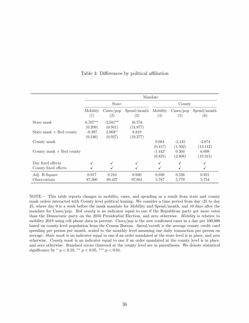
Table 3: Differences by political affiliation

Mandate

State County

Mobility Cases/pop Spend/month Mobility Cases/pop Spend/month(1) (2) (3) (4) (5) (6)

State mask 0.707∗∗∗ -2.581∗∗∗ 16.754(0.209) (0.941) (14.877)

State mask × Red county -0.397 2.069∗∗ 8.819(0.246) (0.927) (19.277)

County mask 0.084 -2.145 -2.874(0.417) (1.502) (13.112)

County mask × Red county -1.442∗ 0.304 6.698(0.825) (2.808) (19.315)

Day fixed effects X X X X X XCounty fixed effects X X X X X X

Adj. R-Square 0.917 0.210 0.930 0.939 0.526 0.921Observations 87,300 99,437 97,801 5,787 5,779 5,754

NOTE.— This table reports changes in mobility, cases, and spending as a result from state and countymask orders interacted with County level political leaning. We consider a time period from day -25 to day25, where day 0 is a week before the mask mandate for Mobility and Spend/month, and 10 days after themandate for Cases/pop. Red county is an indicator equal to one if the Republican party got more votesthan the Democratic party on the 2016 Presidential Election, and zero otherwise. Mobility is relative tomobility 2019 using cell phone data in percent. Cases/pop is the new confirmed cases in a day per 100,000based on county-level population from the Census Bureau. Spend/month is the average county credit cardspending per person per month, scaled to the monthly level assuming one daily transaction per person onaverage. State mask is an indicator equal to one if an order mandated at the state level is in place, and zerootherwise. County mask is an indicator equal to one if an order mandated at the county level is in place,and zero otherwise. Standard errors clustered at the county level are in parentheses. We denote statisticalsignificance by ∗ p < 0.10, ∗∗ p < 0.05, ∗∗∗ p < 0.01.

36

Table 4: Differences by urban and rural counties

Mandate

State County

Mobility Cases/pop Spend/month Mobility Cases/pop Spend/month(1) (2) (3) (4) (5) (6)

State mask 0.469∗∗∗ -0.626 20.967∗∗∗

(0.095) (0.382) (7.299)State mask × Urban county -0.295 -1.230∗∗ 12.772

(0.189) (0.568) (8.729)County mask 1.205 -2.703 26.584

(0.971) (3.074) (28.125)County mask × Urban county -2.274∗ 0.913 -35.524

(1.183) (3.871) (33.684)

Day fixed effects X X X X X XCounty fixed effects X X X X X X

Adj. R-Square 0.917 0.210 0.930 0.940 0.526 0.921Observations 87,300 99,437 97,801 5,787 5,779 5,754

NOTE.— This table reports changes in mobility, cases, and spending as a result from state and county maskorders interacted with County level extent of Urban population. We consider a time period from day -25 today 25, where day 0 is a week before the mask mandate for Mobility and Spend/month, and 10 days afterthe mandate for Cases/pop. Urban county is an indicator equal to one if urban areas include more than 50%of the county population, and zero otherwise. Mobility is relative to mobility 2019 using cell phone datain percent. Cases/pop is the new confirmed cases in a day per 100,000 based on county-level populationfrom the Census Bureau. Spend/month is the average county credit card spending per person per month,scaled to the monthly level assuming one daily transaction per person on average. State mask is an indicatorequal to one if an order mandated at the state level is in place, and zero otherwise. County mask is anindicator equal to one if an order mandated at the county level is in place, and zero otherwise. Standarderrors clustered at the county level are in parentheses. We denote statistical significance by ∗ p < 0.10, ∗∗

p < 0.05, ∗∗∗ p < 0.01.

37

Table 5: Differences by high and low case count counties

Mandate

State County

Mobility Cases/pop Spend/month Mobility Cases/pop Spend/month(1) (2) (3) (4) (5) (6)

State mask 0.735∗∗∗ 1.021∗∗ 16.250∗

(0.125) (0.483) (9.040)State mask × High county -0.628∗∗∗ -3.761∗∗∗ 14.982

(0.176) (0.552) (11.672)County mask 0.730 0.458 -2.230

(0.780) (1.849) (31.467)County mask × High county -1.629∗ -3.258 2.798

(0.941) (2.619) (36.793)

Day fixed effects X X X X X XCounty fixed effects X X X X X X

Adj. R-Square 0.917 0.211 0.930 0.939 0.526 0.921Observations 87,300 99,437 97,801 5,787 5,779 5,754

NOTE.— This table reports changes in mobility, cases, and spending as a result from state and county maskorders interacted with County level case severity. We consider a time period from day -25 to day 25, whereday 0 is a week before the mask mandate for Mobility and Spend/month, and 10 days after the mandatefor Cases/pop. High county is an indicator equal to one if the number of cases on event-day 0 are abovethe median value of event-day 0 values, and zero otherwise. Mobility is relative to mobility 2019 using cellphone data in percent. Cases/pop is the new confirmed cases in a day per 100,000 based on county-levelpopulation from the Census Bureau. Spend/month is the average county credit card spending per person permonth, scaled to the monthly level assuming one daily transaction per person on average. State mask is anindicator equal to one if an order mandated at the state level is in place, and zero otherwise. County mask isan indicator equal to one if an order mandated at the county level is in place, and zero otherwise. Standarderrors clustered at the county level are in parentheses. We denote statistical significance by ∗ p < 0.10, ∗∗

p < 0.05, ∗∗∗ p < 0.01.

38

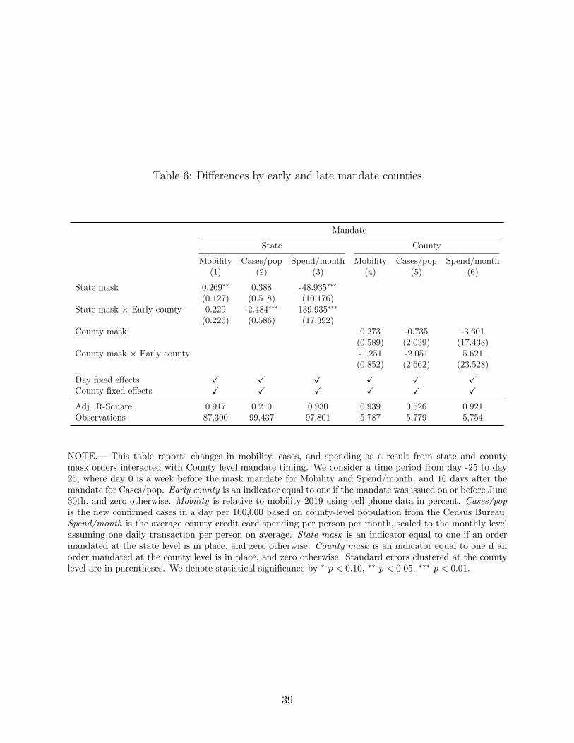
Table 6: Differences by early and late mandate counties

Mandate

State County

Mobility Cases/pop Spend/month Mobility Cases/pop Spend/month(1) (2) (3) (4) (5) (6)

State mask 0.269∗∗ 0.388 -48.935∗∗∗

(0.127) (0.518) (10.176)State mask × Early county 0.229 -2.484∗∗∗ 139.935∗∗∗

(0.226) (0.586) (17.392)County mask 0.273 -0.735 -3.601

(0.589) (2.039) (17.438)County mask × Early county -1.251 -2.051 5.621

(0.852) (2.662) (23.528)

Day fixed effects X X X X X XCounty fixed effects X X X X X X

Adj. R-Square 0.917 0.210 0.930 0.939 0.526 0.921Observations 87,300 99,437 97,801 5,787 5,779 5,754

NOTE.— This table reports changes in mobility, cases, and spending as a result from state and countymask orders interacted with County level mandate timing. We consider a time period from day -25 to day25, where day 0 is a week before the mask mandate for Mobility and Spend/month, and 10 days after themandate for Cases/pop. Early county is an indicator equal to one if the mandate was issued on or before June30th, and zero otherwise. Mobility is relative to mobility 2019 using cell phone data in percent. Cases/popis the new confirmed cases in a day per 100,000 based on county-level population from the Census Bureau.Spend/month is the average county credit card spending per person per month, scaled to the monthly levelassuming one daily transaction per person on average. State mask is an indicator equal to one if an ordermandated at the state level is in place, and zero otherwise. County mask is an indicator equal to one if anorder mandated at the county level is in place, and zero otherwise. Standard errors clustered at the countylevel are in parentheses. We denote statistical significance by ∗ p < 0.10, ∗∗ p < 0.05, ∗∗∗ p < 0.01.

39

Table 7: Differences by compliance to wearing a mask

Mandate

State County

Mobility Cases/pop Spend/month Mobility Cases/pop Spend/month(1) (2) (3) (4) (5) (6)

State mask -0.021 0.024 18.048(0.146) (0.455) (13.034)

State mask × Comply county 0.595∗∗∗ -1.409∗∗ 8.855(0.177) (0.568) (14.700)

County mask 1.897 6.204∗∗ -2.817(1.280) (3.038) (21.079)

County mask × Comply county -2.755∗ -9.442∗∗∗ 3.129(1.425) (3.490) (22.421)

Day fixed effects X X X X X XCounty fixed effects X X X X X X

Adj. R-Square 0.917 0.210 0.930 0.940 0.529 0.921Observations 87,300 99,437 97,801 5,787 5,779 5,754

NOTE.— This table reports changes in mobility, cases, and spending as a result from state and countymask orders interacted with County level mark-wearing compliance, based on responses to a New YorkTimes survey. We consider a time period from day -25 to day 25, where day 0 is a week before the maskmandate for Mobility and Spend/month, and 10 days after the mandate for Cases/pop. Comply county isan indicator equal to one if at 70% of people surveyed stated that they were a mask always or frequently,and zero otherwise. Mobility is relative to mobility 2019 using cell phone data in percent. Cases/pop isthe new confirmed cases in a day per 100,000 based on county-level population from the Census Bureau.Spend/month is the average county credit card spending per person per month, scaled to the monthly levelassuming one daily transaction per person on average. State mask is an indicator equal to one if an ordermandated at the state level is in place, and zero otherwise. County mask is an indicator equal to one if anorder mandated at the county level is in place, and zero otherwise. Standard errors clustered at the countylevel are in parentheses. We denote statistical significance by ∗ p < 0.10, ∗∗ p < 0.05, ∗∗∗ p < 0.01.

40

Table 8: Regression Discontinuity Estimation in Event Time

Mandate

State County

Mobility Cases/pop Spend/month Mobility Cases/pop Spend/month(1) (2) (3) (4) (5) (6)

RD Estimate 0.912∗∗∗ -0.643 131.581∗∗∗ -0.341 -2.174∗ 51.631(0.323) (0.435) (23.371) (0.954) (1.283) (41.010)

Optimal BW 15.1 19.8 28.3 26.0 37.3 22.8Observations 396,565 374,594 361,645 25,688 23,300 22,382

NOTE.— This table reports changes in mobility, cases, and spending in a regression discontinuity frameworkusing event time as the forcing variable. We consider a time period from day -25 to day 25, where day 0 is aweek before the mask mandate for Mobility and Spend/month, and 10 days after the mandate for Cases/pop.Mobility is relative to mobility 2019 using cell phone data in percent. Cases/pop is the new confirmed casesin a day per 100,000 based on county-level population from the Census Bureau. Spend/month is the averagecounty credit card spending per person per month, scaled to the monthly level assuming one daily transactionper person on average. State mask is an indicator equal to one if an order mandated at the state level isin place, and zero otherwise. County mask is an indicator equal to one if an order mandated at the countylevel is in place, and zero otherwise. Standard errors clustered at the county level are in parentheses. Wedenote statistical significance by ∗ p < 0.10, ∗∗ p < 0.05, ∗∗∗ p < 0.01.

41

Table 9: Parametric Event Study with Event Time Controls

Panel A: Linear Event time ControlMandate

State County

Mobility Cases/pop Spend/month Mobility Cases/pop Spend/month(1) (2) (3) (4) (5) (6)

State mask 0.385∗∗∗ -0.916∗∗∗ 23.359∗∗∗

(0.079) (0.337) (6.656)County mask -0.576∗∗ -2.207∗∗ 0.869

(0.223) (1.024) (10.122)

Linear Event-time Controls X X X X X XDay fixed effects X X X X X XCounty fixed effects X X X X X X

Adj. R-Square 0.917 0.209 0.930 0.939 0.527 0.921Observations 87,300 99,437 97,801 5,787 5,779 5,754

Panel B: Cubic Event time ControlMandate

State County

Mobility Cases/pop Spend/month Mobility Cases/pop Spend/month(1) (2) (3) (4) (5) (6)

State mask 0.855∗∗∗ -2.049∗∗∗ 71.251∗∗∗

(0.142) (0.639) (14.413)County mask -1.007∗∗∗ 2.653 31.331

(0.375) (1.672) (22.931)

Cubic Event-time Controls X X X X X XDay fixed effects X X X X X XCounty fixed effects X X X X X X

Adj. R-Square 0.917 0.210 0.930 0.939 0.528 0.921Observations 87,300 99,437 97,801 5,787 5,779 5,754

NOTE.— This table reports changes in mobility, cases, and spending mirroring the specification in Table 2,with the addition of Event Time as a control variable interacted with the State and County mask variables.Panel A includes event time as a linear interacted control, and Panel B includes event time as a linear, second,and third order controls. We consider a time period from day -25 to day 25, where day 0 is a week beforethe mask mandate for Mobility and Spend/month, and 10 days after the mandate for Cases/pop. Mobilityis relative to mobility 2019 using cell phone data in percent. Cases/pop is the new confirmed cases in a dayper 100,000 based on county-level population from the Census Bureau. Spend/month is the average countycredit card spending per person per month, scaled to the monthly level assuming one daily transaction perperson on average. State mask is an indicator equal to one if an order mandated at the state level is in place,and zero otherwise. County mask is an indicator equal to one if an order mandated at the county level isin place, and zero otherwise. Standard errors clustered at the county level are in parentheses. We denotestatistical significance by ∗ p < 0.10, ∗∗ p < 0.05, ∗∗∗ p < 0.01.

42

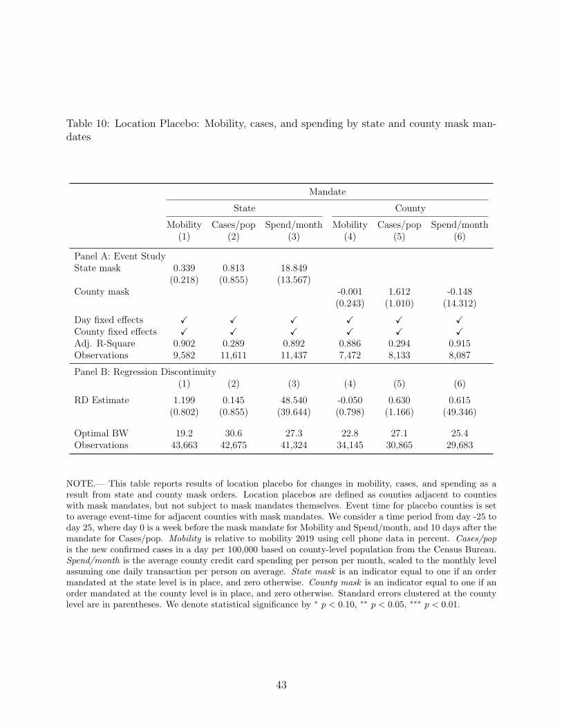
Table 10: Location Placebo: Mobility, cases, and spending by state and county mask man-dates

Mandate

State County

Mobility Cases/pop Spend/month Mobility Cases/pop Spend/month(1) (2) (3) (4) (5) (6)

Panel A: Event StudyState mask 0.339 0.813 18.849

(0.218) (0.855) (13.567)County mask -0.001 1.612 -0.148

(0.243) (1.010) (14.312)

Day fixed effects X X X X X XCounty fixed effects X X X X X XAdj. R-Square 0.902 0.289 0.892 0.886 0.294 0.915Observations 9,582 11,611 11,437 7,472 8,133 8,087

Panel B: Regression Discontinuity(1) (2) (3) (4) (5) (6)

RD Estimate 1.199 0.145 48.540 -0.050 0.630 0.615(0.802) (0.855) (39.644) (0.798) (1.166) (49.346)

Optimal BW 19.2 30.6 27.3 22.8 27.1 25.4Observations 43,663 42,675 41,324 34,145 30,865 29,683

NOTE.— This table reports results of location placebo for changes in mobility, cases, and spending as aresult from state and county mask orders. Location placebos are defined as counties adjacent to countieswith mask mandates, but not subject to mask mandates themselves. Event time for placebo counties is setto average event-time for adjacent counties with mask mandates. We consider a time period from day -25 today 25, where day 0 is a week before the mask mandate for Mobility and Spend/month, and 10 days after themandate for Cases/pop. Mobility is relative to mobility 2019 using cell phone data in percent. Cases/popis the new confirmed cases in a day per 100,000 based on county-level population from the Census Bureau.Spend/month is the average county credit card spending per person per month, scaled to the monthly levelassuming one daily transaction per person on average. State mask is an indicator equal to one if an ordermandated at the state level is in place, and zero otherwise. County mask is an indicator equal to one if anorder mandated at the county level is in place, and zero otherwise. Standard errors clustered at the countylevel are in parentheses. We denote statistical significance by ∗ p < 0.10, ∗∗ p < 0.05, ∗∗∗ p < 0.01.

43

Table 11: Time placebo: Mobility, cases, and spending by state and county mask mandates

Mandate

State County

Mobility Cases/pop Spend/month Mobility Cases/pop Spend/month(1) (2) (3) (4) (5) (6)

Panel A: Event StudyState mask -0.001 -0.139 -15.582

(0.116) (0.421) (11.483)County mask -0.288 -0.451 -0.634

(0.343) (0.397) (19.429)

Day fixed effects X X X X X XCounty fixed effects X X X X X XAdj. R-Square 0.894 0.222 0.860 0.944 0.365 0.908Observations 71,530 59,556 47,843 5,006 4,800 4,033

Panel B: Regression Discontinuity(1) (2) (3) (4) (5) (6)

RD Estimate 0.069 0.545 29.445 0.358 -0.257 -27.501(0.440) (0.409) (38.752) (1.483) (0.450) (57.665)

Optimal BW 10.1 14.9 13.0 13.6 21.3 22.1Observations 396,565 374,594 361,645 25,688 23,300 22,382

NOTE.— This table reports results of a time placebo for changes in mobility, cases, and spending as a resultfrom state and county mask orders. Time placebos are determined by randomly reassigning an event timeat least 75 days before the true event time. Event time for placebo counties is set to average event-timefor adjacent counties with mask mandates. We consider a time period from day -25 to day 25. Mobility isrelative to mobility 2019 using cell phone data in percent. Cases/pop is the new confirmed cases in a dayper 100,000 based on county-level population from the Census Bureau. Spend/month is the average countycredit card spending per person per month, scaled to the monthly level assuming one daily transaction perperson on average. State mask is an indicator equal to one if an order mandated at the state level is in place,and zero otherwise. County mask is an indicator equal to one if an order mandated at the county level isin place, and zero otherwise. Standard errors clustered at the county level are in parentheses. We denotestatistical significance by ∗ p < 0.10, ∗∗ p < 0.05, ∗∗∗ p < 0.01.

44

Table 12: Survey Evidence

How much more or less likely (as a percent) would you be to go out to a store if:

The number of confirmed cases fell by 10% 12.62%(1.49)

The number of confirmed cases fell by 50% 29.62%(1.69)

The number of confirmed cases fell by 90% 56.82%(2.22)

Half of the people were wearing a mask -13.48%(1.93)

Everyone was wearing a mask 50.72%(2.28)

The store enforced wearing a mask 49.73%(2.50)

The state enforced wearing a mask 48.76%(2.79)

Observations 305

NOTE.— Survey evidence from the October and November Utah Consumer Sentiment Survey. Standarderrors in parentheses.

45

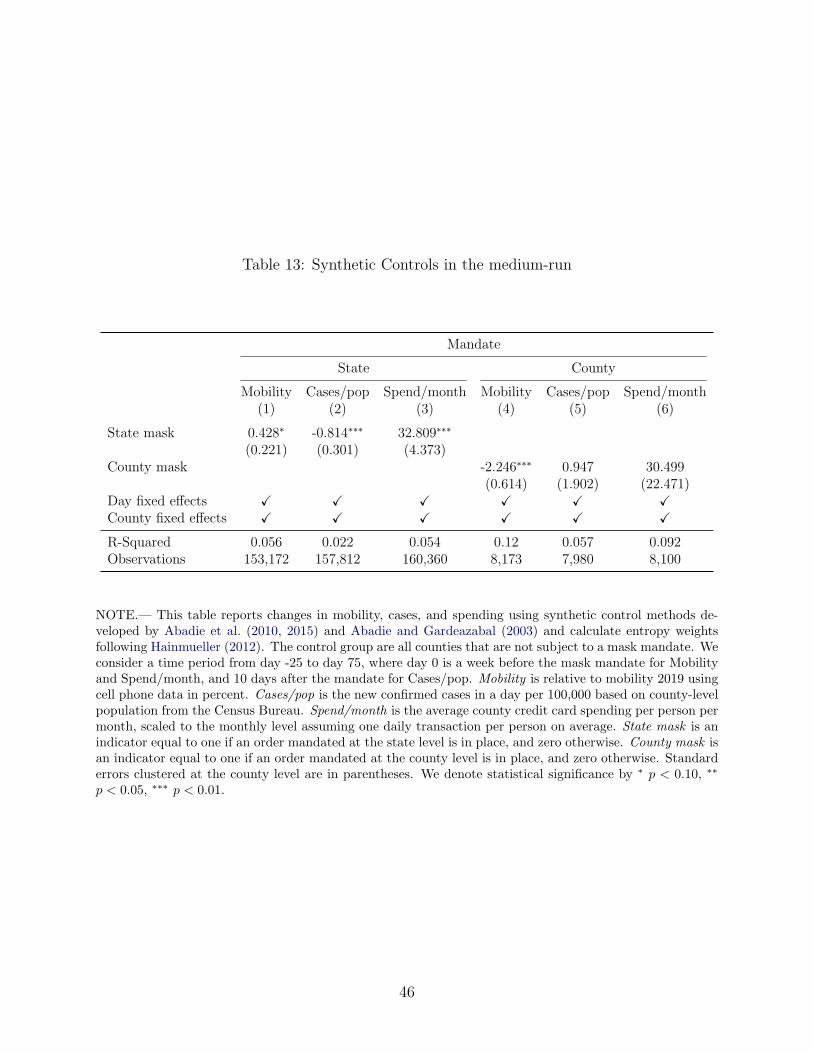
Table 13: Synthetic Controls in the medium-run

Mandate

State County

Mobility Cases/pop Spend/month Mobility Cases/pop Spend/month(1) (2) (3) (4) (5) (6)

State mask 0.428∗ -0.814∗∗∗ 32.809∗∗∗

(0.221) (0.301) (4.373)County mask -2.246∗∗∗ 0.947 30.499

(0.614) (1.902) (22.471)Day fixed effects X X X X X XCounty fixed effects X X X X X X

R-Squared 0.056 0.022 0.054 0.12 0.057 0.092Observations 153,172 157,812 160,360 8,173 7,980 8,100

NOTE.— This table reports changes in mobility, cases, and spending using synthetic control methods de-veloped by Abadie et al. (2010, 2015) and Abadie and Gardeazabal (2003) and calculate entropy weightsfollowing Hainmueller (2012). The control group are all counties that are not subject to a mask mandate. Weconsider a time period from day -25 to day 75, where day 0 is a week before the mask mandate for Mobilityand Spend/month, and 10 days after the mandate for Cases/pop. Mobility is relative to mobility 2019 usingcell phone data in percent. Cases/pop is the new confirmed cases in a day per 100,000 based on county-levelpopulation from the Census Bureau. Spend/month is the average county credit card spending per person permonth, scaled to the monthly level assuming one daily transaction per person on average. State mask is anindicator equal to one if an order mandated at the state level is in place, and zero otherwise. County mask isan indicator equal to one if an order mandated at the county level is in place, and zero otherwise. Standarderrors clustered at the county level are in parentheses. We denote statistical significance by ∗ p < 0.10, ∗∗

p < 0.05, ∗∗∗ p < 0.01.

46

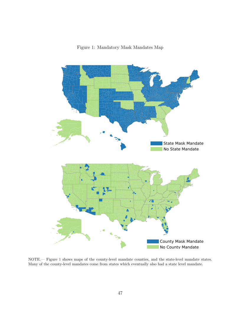
Figure 1: Mandatory Mask Mandates Map

State Mask MandateNo State Mandate

County Mask MandateNo County Mandate

NOTE.— Figure 1 shows maps of the county-level mandate counties, and the state-level mandate states.Many of the county-level mandates come from states which eventually also had a state level mandate.

47

Figure 2: Covid-19 Case Rates in August

0

200

400

600

800

1000

1200

1400

1600

Mask MandateNo Mandate

NOTE.— Figure 2 shows a map of the county-level active coronavirus cases per 100,000 people as of August1st, and under that for comparison, the map of counties and states with any mandate in place (which is thecombination of the State and County maps from Figure 1). Coronavirus case rate data come from the NewYork Times, and population statistics come from the 2019 Census estimate of county level residence.

48

Figure 3: Mobility, cases, and spending around mask mandate for county or state mandates

Mobility State Mandate

-15

-14

-13

-12

-11

-10

Mob

ility

(% c

hang

e fro

m 2

019)

-21 -14 -7 0 7 14 21Days around State Mask-Mandate

Mobility County Mandate

-22

-21

-20

-19

-18

Mob

ility

(% c

hang

e fro

m 2

019)

-21 -14 -7 0 7 14 21Days around County Mask-Mandate

Cases State Mandate

810

1214

16D

aily

New

Cas

es /

100,

000

-21 -14 -7 0 7 14 21Days around State Mask-Mandate

Cases County Mandate

1520

2530

35D

aily

New

Cas

es /

100,

000

-21 -14 -7 0 7 14 21Days around County Mask-Mandate

Spending State Mandate

1000

1100

1200

1300

1400

1500

Dai

ly S

pend

ing

/ per

son

(in m

onth

ly $

)

-21 -14 -7 0 7 14 21Days around State Mask-Mandate

Event Day Average Fit Linear Estimation

Spending County Mandate

700

800

900

1000

1100

Dai

ly S

pend

ing

/ per

son

(in m

onth

ly $

)

-21 -14 -7 0 7 14 21Days around County Mask-Mandate

Event Day Average Fit Linear Estimation

NOTE.— Figure 3 shows how mobility, cases per 100,000 people, and spending per person per month changearound the implementation of a mandate.

49

Figure 4: Medium-Run Synthetic Controls

Mobility State Mandate Mobility County Mandate

Cases State Mandate Cases County Mandate

Spending State Mandate Spending County Mandate

NOTE.— Figure 4 shows how mobility, cases per 100,000 people, and spending per person per month changearound the implementation of a mandate.

50

Appendix A Survey data

The survey evidence we report in Section 7.1 is from a short survey we conducted in con-junction with the State of Utah on consumer sentiment.12 Participants were recruited bymail and included a link to a survey. We selected addresses from a database of all addressesin the state of Utah. We recruited a representative sample of Utah by selecting addressesbased on nonresponse rates from previous surveys the HERO project conducted (Gaulin etal., 2020). For example, we over sampled census block groups with lower income and a higherpercentage of Hispanics to ensure our resulting survey was representative of the populationof Utah.

We pooled the answers from the October and the November waves of the survey. Partic-ipants were paid $10 to take the survey in the November wave.

Utah as a state is more white, less Hispanic, has a higher median income, and slightlylower percentage with a bachelor’s degree or higher than the US. Our survey participants hada similar white percentage and median income to Utah’s population but were less Hispanicand had higher education attainment.

Population Survey

White 90% 87%Hispanic 14% 11%Median income $68,374 $50,000–$74,999Bachelor’s or higher 33% 50%

Appendix B Joint Estimation of Heterogeneous Treat-

ment Effects

In this section we document that almost all of our analysis of treatment effect heterogeneityfrom section 5 is robust to joint estimation of all interaction effects. Since most of theanalyzed effects remain qualitatively and quantitatively similar, we focus here and just threeinteractions that are affected by the joint estimation.

The comparison of table A.3 with the results in table 4 shows that the joint analysis ofall interaction terms shifts some of the effects of urban counties. For example, responses ofcase growth to state mask mandates fall by about 60% and become insignificant in the jointanalysis. At the same time, the response of case growth to county mask mandates turnsstrongly positive and significant. This suggests that the mobility decline through countymask mandates is insufficient to offset higher virus exposure in denser areas.

Additionally, the joint analysis of all interaction terms renders the response of earlycounties to state mask mandates insignificant. This is most likely related to the fact thatearly counties with mask mandates were primarily in urban and liberal areas.

12As part of the HERO project, University of Utah faculty worked with the State of Utah to provideanswers about COVID-19. https://eccles.utah.edu/utah-health-economic-recovery-outreach/

51

Appendix C Differences-in-Differences Approach

This appendix extends our analysis to the medium-run using a difference-in-differences ap-proach. In Table A.4 and Figure A.7, we report estimates from a differences-in-differencesanalysis. The short-run estimates rely on the identifying assumption that all omitted vari-ables are continuous around the time of the mask mandate. This assumption becomes lesstenable in the medium-run. To control for potential conflating factors, we rely on a controlgroup of counties adjacent to counties that are ever subject to a county or state mask man-date. We assign an event time to the control counties equal to that of the adjacent countysubject to a mask mandate. This differences-in-differences specification relies on the paralleltrend assumption, which we investigate in Figure A.7. We find no evidence of differentialtrends for any of our dependent variables before a government enacts a mask mandate. Acontrol group allows us to estimate up to 75 days after a government enacts a mask mandate.

We also note that control counties’ geographic adjacency to treatment counties is likelyto bias our estimates against finding results. This bias is the result of possible spilloversacross adjacent counties. For example, suppose as a result of a mask mandate in county A,people in the adjacent county B also increase their mobility. Our differences-in-differencesstrategy can only identify the difference between the mobility increase in county A andcounty B, which is smaller than the absolute value for the mobility increase in county A.Similar arguments can be made for spillovers in spending or case growth.

The impact of state mask mandates on mobility and case growth is 4−5× larger than theimmediate short-run impact we report in Table 2. Specifically, in column (1) of Table A.4,we report that mobility is 1.3 percentage points higher after a state enacts a mask mandateand cases are lower by five people per 100,000. These results confirm that the treatmenteffects of state mask mandates are persistent and accumulate over time, as would be thecase if mask mandates can consistently impact the trajectory of COVID-19 infection risk.

The opposite dynamic is at work in counties with county-only mask mandates. We report,in the last three columns of Table A.4, that mobility strongly increases over the medium-run, after immediately dropping as documented in Table 2. This transitory negative effectis consistent with the view that information effects are transient in nature and that themedium-run effects of mask orders are qualitatively the same for state and county maskmandates.

52

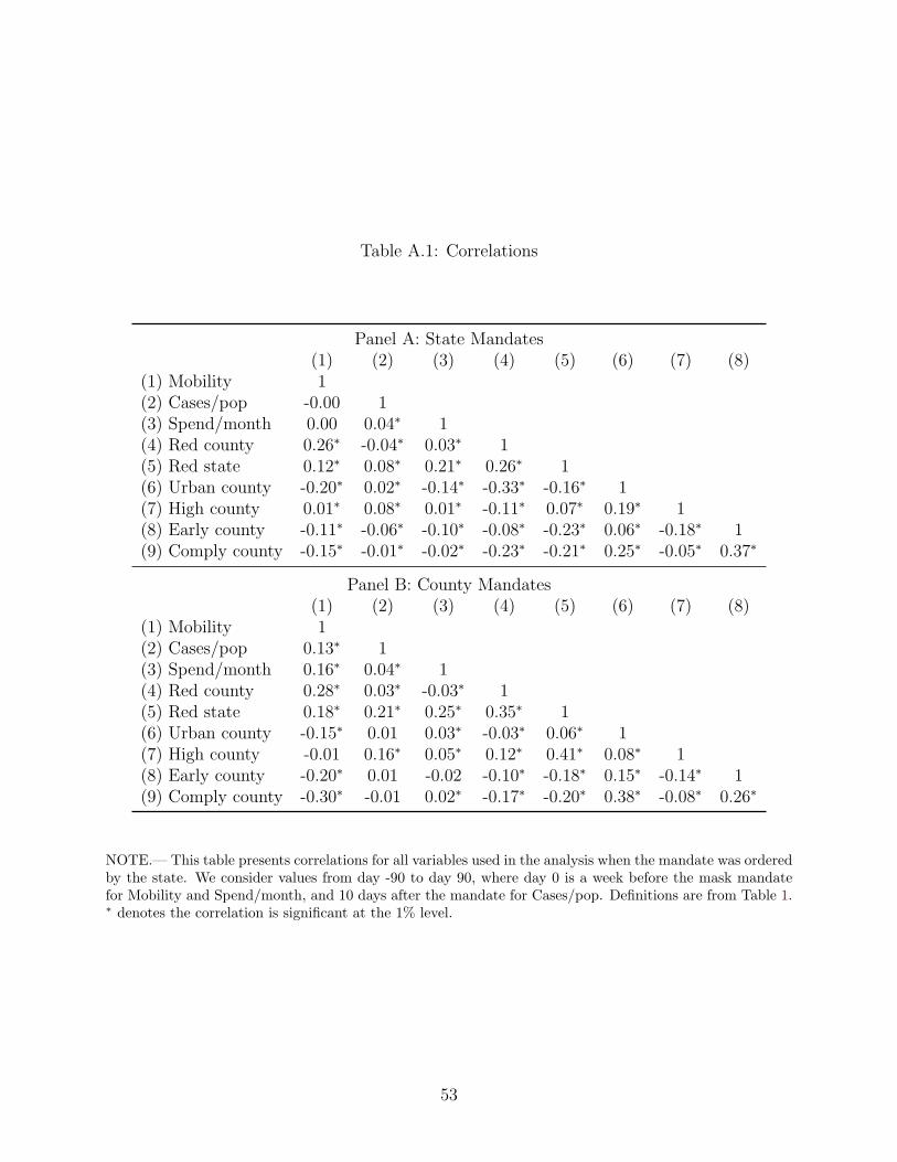
Table A.1: Correlations

Panel A: State Mandates(1) (2) (3) (4) (5) (6) (7) (8)

(1) Mobility 1(2) Cases/pop -0.00 1(3) Spend/month 0.00 0.04∗ 1(4) Red county 0.26∗ -0.04∗ 0.03∗ 1(5) Red state 0.12∗ 0.08∗ 0.21∗ 0.26∗ 1(6) Urban county -0.20∗ 0.02∗ -0.14∗ -0.33∗ -0.16∗ 1(7) High county 0.01∗ 0.08∗ 0.01∗ -0.11∗ 0.07∗ 0.19∗ 1(8) Early county -0.11∗ -0.06∗ -0.10∗ -0.08∗ -0.23∗ 0.06∗ -0.18∗ 1(9) Comply county -0.15∗ -0.01∗ -0.02∗ -0.23∗ -0.21∗ 0.25∗ -0.05∗ 0.37∗

Panel B: County Mandates(1) (2) (3) (4) (5) (6) (7) (8)

(1) Mobility 1(2) Cases/pop 0.13∗ 1(3) Spend/month 0.16∗ 0.04∗ 1(4) Red county 0.28∗ 0.03∗ -0.03∗ 1(5) Red state 0.18∗ 0.21∗ 0.25∗ 0.35∗ 1(6) Urban county -0.15∗ 0.01 0.03∗ -0.03∗ 0.06∗ 1(7) High county -0.01 0.16∗ 0.05∗ 0.12∗ 0.41∗ 0.08∗ 1(8) Early county -0.20∗ 0.01 -0.02 -0.10∗ -0.18∗ 0.15∗ -0.14∗ 1(9) Comply county -0.30∗ -0.01 0.02∗ -0.17∗ -0.20∗ 0.38∗ -0.08∗ 0.26∗

NOTE.— This table presents correlations for all variables used in the analysis when the mandate was orderedby the state. We consider values from day -90 to day 90, where day 0 is a week before the mask mandatefor Mobility and Spend/month, and 10 days after the mandate for Cases/pop. Definitions are from Table 1.∗ denotes the correlation is significant at the 1% level.

53

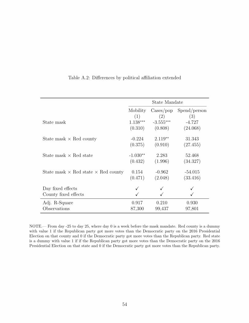
Table A.2: Differences by political affiliation extended

State Mandate

Mobility Cases/pop Spend/person(1) (2) (3)

State mask 1.138∗∗∗ -3.555∗∗∗ -4.727(0.310) (0.808) (24.068)

State mask × Red county -0.224 2.119∗∗ 31.343(0.375) (0.910) (27.455)

State mask × Red state -1.030∗∗ 2.283 52.468(0.432) (1.996) (34.327)

State mask × Red state × Red county 0.154 -0.962 -54.015(0.471) (2.048) (33.416)

Day fixed effects X X XCounty fixed effects X X X

Adj. R-Square 0.917 0.210 0.930Observations 87,300 99,437 97,801

NOTE.— From day -25 to day 25, where day 0 is a week before the mask mandate. Red county is a dummywith value 1 if the Republican party got more votes than the Democratic party on the 2016 PresidentialElection on that county and 0 if the Democratic party got more votes than the Republican party. Red stateis a dummy with value 1 if if the Republican party got more votes than the Democratic party on the 2016Presidential Election on that state and 0 if the Democratic party got more votes than the Republican party.

54

Table A.3: Mobility, cases, and spending by state and county mask mandates

Mandate

State County

Mobility Cases/pop Spend/month Mobility Cases/pop Spend/month(1) (2) (3) (4) (5) (6)

State mask 0.795∗∗ 1.740 -73.477∗∗∗

(0.318) (1.307) (25.086)State mask × Red county -0.502∗ 1.425 15.635

(0.276) (1.014) (21.528)State mask × Urban county -0.459∗∗ 0.448 11.317

(0.221) (0.707) (12.067)State mask × High county -0.599∗∗∗ -3.799∗∗∗ 20.878∗

(0.184) (0.576) (11.972)State mask × Early county 0.028 -2.757∗∗∗ 143.021∗∗∗

(0.239) (0.633) (18.995)State mask × Comply county 0.619∗∗∗ -0.779 -4.487

(0.189) (0.598) (15.790)County mask 4.922∗∗∗ 8.698∗∗ -3.003

(1.619) (4.336) (41.614)County mask × Red county -1.541∗ -0.465 8.536

(0.794) (2.686) (19.056)County mask × Urban county -1.442 4.556 -43.610

(1.175) (4.015) (36.012)County mask × High county -1.470 -3.973 7.898

(0.894) (2.466) (33.439)County mask × Early county -1.026 -1.334 7.688

(0.797) (2.916) (22.718)County mask × Comply county -2.226∗ -11.572∗∗∗ 24.358

(1.307) (4.029) (29.267)

Day fixed effects X X X X X XCounty fixed effects X X X X X X

Adj. R-Square 0.917 0.211 0.930 0.941 0.531 0.921Observations 87,300 99,437 97,801 5,787 5,779 5,754

NOTE.— This table reports changes in mobility, cases, and spending as a result from state and countymask orders. We consider a time period from day -25 to day 25, where day 0 is a week before the maskmandate for Mobility and Spend/month, and 10 days after the mandate for Cases/pop. Mobility is relativeto mobility 2019 using cell phone data in percent. Cases/pop is the new confirmed cases in a day per 100,000based on county-level population from the Census Bureau. Spend/month is the average county credit cardspending per person per month, scaled to the monthly level assuming one daily transaction per person onaverage. State mask is an indicator equal to one if an order mandated at the state level is in place, and zerootherwise. County mask is an indicator equal to one if an order mandated at the county level is in place,and zero otherwise. Standard errors clustered at the county level are in parentheses. We denote statisticalsignificance by ∗ p < 0.10, ∗∗ p < 0.05, ∗∗∗ p < 0.01.

55

Table A.4: Differences-in-Differences in the medium-run

Mandate

State County

Mobility Cases/pop Spend/month Mobility Cases/pop Spend/month(1) (2) (3) (4) (5) (6)

State mask 1.259** -5.179*** 10.592(0.572) (1.155) (20.631)

County mask 2.746*** -0.457 121.978***(1.024) (1.726) (33.270)

Day fixed effects X X X X X XCounty fixed effects X X X X X X

R-Square 0.394 0.107 0.868 0.552 0.191 0.819Observations 284,124 307,265 301,034 38,245 38,234 38,723

NOTE.— This table reports changes in mobility, cases, and spending in a differences-in-differences frameworkusing event time and whether the county has a mask mandate as the two dimensions. The control groupare all counties that are adjacent to treated counties that do not ever have a mask mandate. We considera time period from day -75 to day 75, where day 0 is a week before the mask mandate for Mobility andSpend/month, and 10 days after the mandate for Cases/pop. Mobility is relative to mobility 2019 using cellphone data in percent. Cases/pop is the new confirmed cases in a day per 100,000 based on county-levelpopulation from the Census Bureau. Spend/month is the average county credit card spending per person permonth, scaled to the monthly level assuming one daily transaction per person on average. State mask is anindicator equal to one if an order mandated at the state level is in place, and zero otherwise. County mask isan indicator equal to one if an order mandated at the county level is in place, and zero otherwise. Standarderrors clustered at the county level are in parentheses. We denote statistical significance by ∗ p < 0.10, ∗∗

p < 0.05, ∗∗∗ p < 0.01.

56

Figure A.1: Mobility, cases, and spending around mask mandate for county or state mandatesby political affiliation

Mobility in Red County

-13

-12

-11

-10

-9-8

Mob

ility

(% c

hang

e fro

m 2

019)

-21 -14 -7 0 7 14 21Days around State Mask-Mandate

Mobility in Blue County

-26

-24

-22

-20

-18

Mob

ility

(% c

hang

e fro

m 2

019)

-21 -14 -7 0 7 14 21Days around State Mask-Mandate

Cases in Red County

810

1214

16D

aily

New

Cas

es /

100,

000

-21 -14 -7 0 7 14 21Days around State Mask-Mandate

Cases in Blue County

1015

2025

Dai

ly N

ew C

ases

/ 10

0,00

0

-21 -14 -7 0 7 14 21Days around State Mask-Mandate

Spending in Red County

1000

1100

1200

1300

1400

1500

Dai

ly S

pend

ing

/ per

son

(in m

onth

ly $

)

-21 -14 -7 0 7 14 21Days around State Mask-Mandate

Event Day Average Fit Linear Estimation

Spending in Blue County

1000

1100

1200

1300

1400

1500

Dai

ly S

pend

ing

/ per

son

(in m

onth

ly $

)

-21 -14 -7 0 7 14 21Days around State Mask-Mandate

Event Day Average Fit Linear Estimation

NOTE.— Figure A.1 shows how mobility, cases per 100,000 people, and spending per person per monthchange around the implementation of a state mandate, differentiated by average State political affiliation ofthe county (Red or Blue for majority conservative and majority non-conservative respectively.

57

Figure A.2: Mobility, cases, and spending around mask mandate for county or state mandatesby urban vs rural

Mobility in Urban County

-20

-19

-18

-17

-16

-15

Mob

ility

(% c

hang

e fro

m 2

019)

-21 -14 -7 0 7 14 21Days around State Mask-Mandate

Mobility in Rural County

-13

-12

-11

-10

-9-8

Mob

ility

(% c

hang

e fro

m 2

019)

-21 -14 -7 0 7 14 21Days around State Mask-Mandate

Cases in Urban County

1012

1416

18D

aily

New

Cas

es /

100,

000

-21 -14 -7 0 7 14 21Days around State Mask-Mandate

Cases in Rural County

810

1214

Dai

ly N

ew C

ases

/ 10

0,00

0

-21 -14 -7 0 7 14 21Days around State Mask-Mandate

Spending in Urban County

750

800

850

900

950

1000

Dai

ly S

pend

ing

/ per

son

(in m

onth

ly $

)

-21 -14 -7 0 7 14 21Days around State Mask-Mandate

Event Day Average Fit Linear Estimation

Spending in Rural County

1100

1200

1300

1400

1500

1600

Dai

ly S

pend

ing

/ per

son

(in m

onth

ly $

)

-21 -14 -7 0 7 14 21Days around State Mask-Mandate

Event Day Average Fit Linear Estimation

NOTE.— Figure A.2 shows how mobility, cases per 100,000 people, and spending per person per monthchange around the implementation of a state mandate, differentiated by whether the majority of populationlives in an urban center.

58

Figure A.3: Mobility, cases, and spending around mask mandate for county or state mandatesby infection severity

Mobility in High County

-14

-13

-12

-11

-10

Mob

ility

(% c

hang

e fro

m 2

019)

-21 -14 -7 0 7 14 21Days around State Mask-Mandate

Mobility in Low County

-16

-14

-12

-10

-8M

obilit

y (%

cha

nge

from

201

9)

-21 -14 -7 0 7 14 21Days around State Mask-Mandate

Cases in High County

1012

1416

1820

Dai

ly N

ew C

ases

/ 10

0,00

0

-21 -14 -7 0 7 14 21Days around State Mask-Mandate

Cases in Low County

05

1015

Dai

ly N

ew C

ases

/ 10

0,00

0

-21 -14 -7 0 7 14 21Days around State Mask-Mandate

Spending in High County

900

1000

1100

1200

1300

1400

Dai

ly S

pend

ing

/ per

son

(in m

onth

ly $

)

-21 -14 -7 0 7 14 21Days around State Mask-Mandate

Event Day Average Fit Linear Estimation

Spending in Low County

1100

1200

1300

1400

1500

Dai

ly S

pend

ing

/ per

son

(in m

onth

ly $

)

-21 -14 -7 0 7 14 21Days around State Mask-Mandate

Event Day Average Fit Linear Estimation

NOTE.— Figure A.3 shows how mobility, cases per 100,000 people, and spending per person per monthchange around the implementation of a state mandate, differentiated by whether the county had abovemedian event-day 0 new cases per 100,000.

59

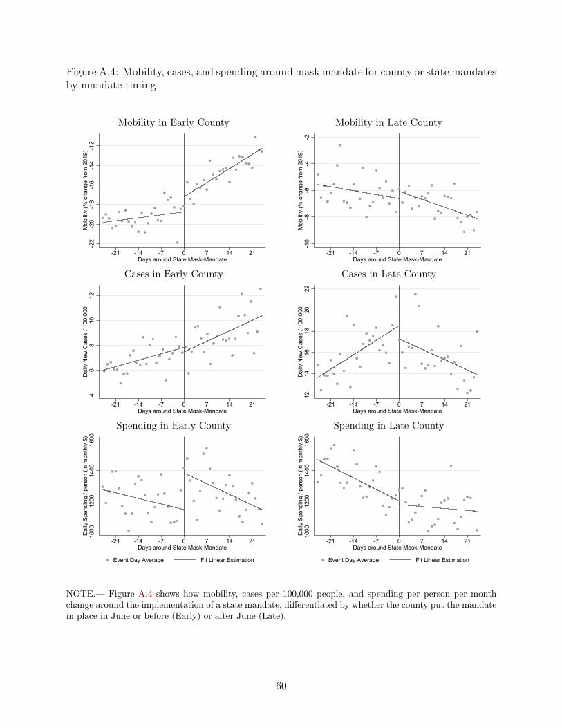
Figure A.4: Mobility, cases, and spending around mask mandate for county or state mandatesby mandate timing

Mobility in Early County

-22

-20

-18

-16

-14

-12

Mob

ility

(% c

hang

e fro

m 2

019)

-21 -14 -7 0 7 14 21Days around State Mask-Mandate

Mobility in Late County

-10

-8-6

-4-2

Mob

ility

(% c

hang

e fro

m 2

019)

-21 -14 -7 0 7 14 21Days around State Mask-Mandate

Cases in Early County

46

810

12D

aily

New

Cas

es /

100,

000

-21 -14 -7 0 7 14 21Days around State Mask-Mandate

Cases in Late County

1214

1618

2022

Dai

ly N

ew C

ases

/ 10

0,00

0

-21 -14 -7 0 7 14 21Days around State Mask-Mandate

Spending in Early County

1000

1200

1400

1600

Dai

ly S

pend

ing

/ per

son

(in m

onth

ly $

)

-21 -14 -7 0 7 14 21Days around State Mask-Mandate

Event Day Average Fit Linear Estimation

Spending in Late County

1000

1200

1400

1600

Dai

ly S

pend

ing

/ per

son

(in m

onth

ly $

)

-21 -14 -7 0 7 14 21Days around State Mask-Mandate

Event Day Average Fit Linear Estimation

NOTE.— Figure A.4 shows how mobility, cases per 100,000 people, and spending per person per monthchange around the implementation of a state mandate, differentiated by whether the county put the mandatein place in June or before (Early) or after June (Late).

60

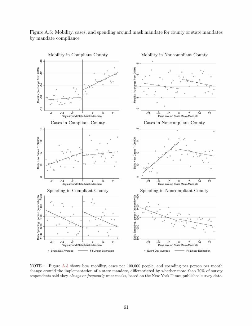
Figure A.5: Mobility, cases, and spending around mask mandate for county or state mandatesby mandate compliance

Mobility in Compliant County

-18

-16

-14

-12

-10

Mob

ility

(% c

hang

e fro

m 2

019)

-21 -14 -7 0 7 14 21Days around State Mask-Mandate

Mobility in Noncompliant County

-9-8

-7-6

-5M

obilit

y (%

cha

nge

from

201

9)

-21 -14 -7 0 7 14 21Days around State Mask-Mandate

Cases in Compliant County

810

1214

16D

aily

New

Cas

es /

100,

000

-21 -14 -7 0 7 14 21Days around State Mask-Mandate

Cases in Noncompliant County

810

1214

16D

aily

New

Cas

es /

100,

000

-21 -14 -7 0 7 14 21Days around State Mask-Mandate

Spending in Compliant County

1100

1200

1300

1400

1500

Dai

ly S

pend

ing

/ per

son

(in m

onth

ly $

)

-21 -14 -7 0 7 14 21Days around State Mask-Mandate

Event Day Average Fit Linear Estimation

Spending in Noncompliant County

800

1000

1200

1400

1600

Dai

ly S

pend

ing

/ per

son

(in m

onth

ly $

)

-21 -14 -7 0 7 14 21Days around State Mask-Mandate

Event Day Average Fit Linear Estimation

NOTE.— Figure A.5 shows how mobility, cases per 100,000 people, and spending per person per monthchange around the implementation of a state mandate, differentiated by whether more than 70% of surveyrespondents said they always or frequently wear masks, based on the New York Times published survey data.

61

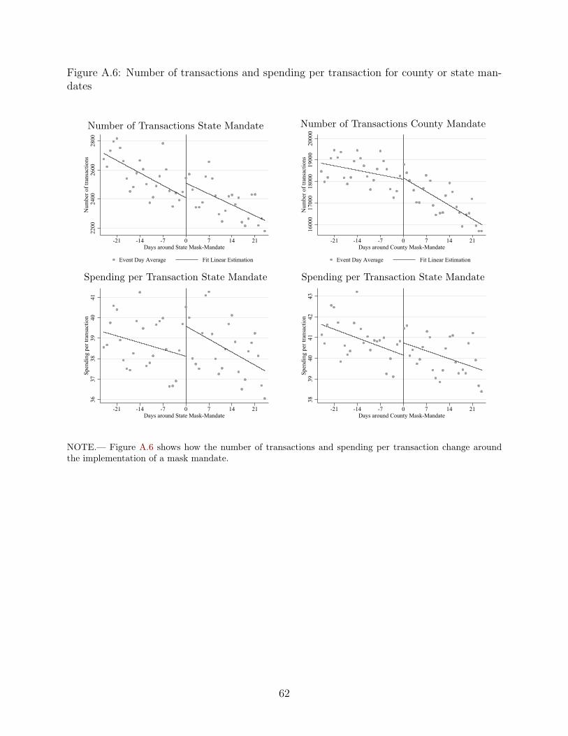
Figure A.6: Number of transactions and spending per transaction for county or state man-dates

Number of Transactions State Mandate

2200

2400

2600

2800

Num

ber o

f tra

nsac

tions

-21 -14 -7 0 7 14 21Days around State Mask-Mandate

Event Day Average Fit Linear Estimation

Number of Transactions County Mandate

1600

017

000

1800

019

000

2000

0N

umbe

r of t

rans

actio

ns

-21 -14 -7 0 7 14 21Days around County Mask-Mandate

Event Day Average Fit Linear Estimation

Spending per Transaction State Mandate

3637

3839

4041

Spen

ding

per

tran

sact

ion

-21 -14 -7 0 7 14 21Days around State Mask-Mandate

Spending per Transaction State Mandate

3839

4041

4243

Spen

ding

per

tran

sact

ion

-21 -14 -7 0 7 14 21Days around County Mask-Mandate

NOTE.— Figure A.6 shows how the number of transactions and spending per transaction change aroundthe implementation of a mask mandate.

62

Figure A.7: Mobility, cases, and spending around mask mandate for county or state mandatescompared to adjacent non-mandate counties

Mobility State Mandate

-50

510

15M

obilit

y (%

cha

nge

from

con

trol)

-25 0 25 50 75Days around state mask order

Mobility County Mandate

-50

510

15M

obilit

y (%

cha

nge

from

con

trol)

-25 0 25 50 75Days around county mask order

Cases State Mandate

-20

-10

010

Dai

ly N

ew C

ases

/ 10

0,00

0

-25 0 25 50 75Days around state mask order

Cases County Mandate

-40

-20

020

Dai

ly N

ew C

ases

/ 10

0,00

0

-25 0 25 50 75Days around county mask order

Spending State Mandate

-400

-200

020

040

0D

aily

Spe

ndin

g / p

erso

n (in

mon

thly

$)

-25 0 25 50 75Days around state mask order

DD Coefficient 95% Confidence Interval

Spending County Mandate

-200

020

040

0D

aily

Spe

ndin

g / p

erso

n (in

mon

thly

$)

-25 0 25 50 75Days around county mask order

DD Coefficient 95% Confidence Interval

NOTE.— Figure A.7 shows how mobility, cases per 100,000 people, and spending per person per monthchange around the implementation of a mandate compared to a set of geographically adjacent control coun-ties.

63