information, hedging demand, and institutional investors: evidence from the taiwan futures exchange

J. of Multi. Fin. Manag. 23 (2013) 394– 414

Contents lists available at ScienceDirect

Journal of Multinational FinancialManagement

journal homepage: www.elsevier.com/locate/econbase

Information, hedging demand, and institutionalinvestors: Evidence from the Taiwan FuturesExchange

Cheng-Yi Chiena,∗, Hsiu-Chuan Leeb, Shih-Wen Taic,Tzu-Hsiang Liaob

a Department of Finance, Feng Chia University, Taichung, Taiwanb Department of Finance, Ming Chuan University, Taipei, Taiwanc Department of Business Administration, Lunghwa University of Science and Technology, Taoyuan, Taiwan

a r t i c l e i n f o

Article history:Received 21 November 2012Accepted 2 August 2013Available online 13 August 2013

JEL classification:G12G14G15

Keywords:InformationHedging demandInstitutional investorsFutures marketGlobal financial turmoil

a b s t r a c t

This paper examines the effect of hedging demand by varioustypes of institutional investor on subsequent returns and volatility.Using data from the Taiwan Futures Exchange, empirical resultsindicate that the hedging demand of foreign investors has a sig-nificant negative impact on subsequent returns and volatility. Inaddition, trading strategies based on the extreme hedging demandof foreigners are positively correlated with trading performance.Furthermore, there is evidence to show that returns (volatility) alsoaffect the subsequent hedging demand of foreign investors, sug-gesting a feedback relation. Finally, the hedging demand of foreigninvestors has a greater impact on subsequent returns and volatil-ity after global financial turmoil. Accordingly, this paper concludesthat foreign investors are informed hedgers in the Taiwan futuresmarket, especially after global financial turmoil.

© 2013 Elsevier B.V. All rights reserved.

1. Introduction

This paper examines the effect of hedging demand by various types of institutional investor onsubsequent returns and volatility. A growing body of literature investigates investor flows of insti-tutional investors in stock markets (e.g., Brennan and Cao, 1997; Bae et al., 2008; Boyer and Zheng,

∗ Corresponding author. Tel.: +886 4 2451 7250x4172; fax: +886 4 2451 3796.E-mail address: [email protected] (C.-Y. Chien).

1042-444X/$ – see front matter © 2013 Elsevier B.V. All rights reserved.http://dx.doi.org/10.1016/j.mulfin.2013.08.001

dx.doi.org/10.1016/j.mulfin.2013.08.001

http://www.sciencedirect.com/science/journal/1042444X

http://www.elsevier.com/locate/econbase

http://crossmark.crossref.org/dialog/?doi=10.1016/j.mulfin.2013.08.001&domain=pdf

mailto:[email protected]

dx.doi.org/10.1016/j.mulfin.2013.08.001

C.-Y. Chien et al. / J. of Multi. Fin. Manag. 23 (2013) 394– 414 395

2009; Bailey et al., 2009). Furthermore, previous research examines the impact of trading demand ofspeculators and hedgers on returns (e.g., Wang, 2003) and volatility (e.g., Wang, 2002). In particular, deRoon et al. (2000) provide evidence that hedging demand affects subsequent futures and spot returns.Despite this evidence, the existing literature does not consider how hedging demand by various typesof institutional investor affects subsequent returns and volatility for futures and spot markets. Hence,this paper seeks to address this gap in the literature.

The relationship between institutional investment flows and stock returns receives much attention.For stock markets, Grinblatt and Keloharju (2000) and Froot et al. (2001) find that the relationshipbetween foreign investment flows and host-country stock returns is positive, thereby implying thatforeign investors possess more information on local stocks than domestic investors. Boyer and Zheng(2009) report that the investor flows of foreigners and mutual funds have a significant impact onstock returns at the quarterly frequency. For the option market, Chang et al. (2009) find that foreigninvestment flows have a greater predictive power with regard to near-the-money and middle-horizonoptions than other institutional investment flows.1 While previous literature investigates the impact ofinstitutional investment flows regarding stock and option markets on stock returns, no work examinesthe impact of institutional investor flows of futures markets on returns and volatility. Since April 7,2008, the Taiwan Futures Exchange (TAIFEX) has published the trading volume and open interestfor foreigners, proprietary traders and mutual funds. These unique data provide an opportunity toexamine this issue.

This paper uses hedging demand as a proxy of investor flows and examines the effect of institutionalinvestor hedging demand on subsequent returns and volatility. Institutional investors can be regardedas informed hedgers if their hedging demand is significantly negative correlated with subsequentreturns (Working, 1953) as well as volatility (Hellwig, 1980; Wang, 1993). Empirical results show thatthe hedging demand of foreigners is significantly negatively related to subsequent futures and spotreturns. In contrast, the hedging demands of proprietary traders and mutual funds are insignificantlynegatively correlated with subsequent futures and spot returns. Furthermore, the hedging demandof foreigners is significantly negatively correlated with subsequent futures and spot volatility. On thecontrary, the hedging demands of proprietary traders and mutual funds are significantly positivelycorrelated with subsequent futures and spot volatility. In addition, the total cumulative futures andspot returns based on the extreme hedging demand of foreigners are positive and largest over theholding period. Furthermore, there is evidence that returns (volatility) also affect the subsequenthedging demand of foreign investors, suggesting a feedback relation. Finally, the hedging demand offoreign investors has more impact on subsequent returns and volatility after global financial turmoil.Overall, this paper concludes that foreign investors are informed hedgers in the Taiwan futures market,especially after global financial turmoil. The results are consistent with Chou and Wang (2009), in thatforeign investors are better informed than other institutional investors.2

Our contribution to the existing literature is two-fold. First, to our knowledge, this is the firststudy of the effect of institutional investment flows with regards to hedging demand on subsequentreturns and volatility in futures markets. This paper complements the existing literature regarding theinvestor flows of institutional investors in the derivatives markets. Second, this paper relates to theinvestment community that the extreme hedging demand of foreign investors is positively correlatedwith trading performance. Intraday data with trader types is not available for practitioners in theTAIFEX. Nevertheless, the TAIFEX publishes the daily trading activity for various types of institutionaltraders. As the data used in this study are daily data and are available for practitioners, strategic traderscan develop a trading strategy according to the extreme hedging demand of foreign investors.

1 Chang et al. (2009) examine the predictive power of the put and call positions of different types of traders in the Taiwanoption market.

2 Chou and Wang (2009) explore the strategic order-splitting behavior and order aggressiveness of different types of tradersusing a dataset of the Taiwan Futures Exchange. This paper differs from Chou and Wang (2009), in that whereas Chou and Wang(2009) investigated the strategic order-splitting behavior using a unique intraday data, this study uses daily data to investigatethe effect of hedging demand by various types of institutional investors on subsequent returns and volatility.

396 C.-Y. Chien et al. / J. of Multi. Fin. Manag. 23 (2013) 394– 414

The remainder of this article is organized as follows. Section 2 presents a literature review. Section 3introduces the theoretical considerations. The data, methodology, and empirical results are presentedin Sections 4–6. The last section presents the conclusions.

2. Literature review

In the finance literature, previous studies investigate the impact of the hedging (trading) demandon futures returns. Bessembinder (1992) indicates that hedging pressure is an important variable as adeterminant of futures risk premiums. Furthermore, de Roon et al. (2000) present a simple model toexplain the relationship between futures risk premiums and hedging demand. de Roon et al. (2000)find that futures risk premiums not only depend on own market hedging pressure but also on cross-market hedging pressures. Wang (2003) investigates the effect of trading demand by different typesof traders on subsequent futures returns, and find that trades of speculators (hedgers) are positively(negatively) associated with subsequent futures returns.3,4 Wang (2003) concludes that this findingsupports the argument of hedging pressure effects.

Additionally, previous research examines the relationship between hedging (trading) demand byvarious types of traders and market volatility. Bessembinder and Seguin (1993) suggest that the rela-tionship between trading activity and volatility may depend on the type of trader. Chang et al. (2000)examine the relationship between stock market volatility and the demand for hedging in S&P 500index futures contracts. Using open interest as a proxy for hedging demand, Chang et al. (2000) find apositively significant relationship between daily open interest of hedgers and stock market volatility,and no significant relationship between daily open interest of speculators and stock market volatil-ity. Wang (2002) investigates the relationship between futures price volatility and trading demandby type of trader in the S&P 500 index futures market.5 Wang (2002) finds that volatility co-variesnegatively with unexpected speculative trading demand (trading demand of speculators), but is posi-tively related to unexpected hedging demand (trading demand of hedgers), thus suggesting that largerspeculators (hedgers) are informed traders (uninformed traders). Pan et al. (2003) examine how mar-ket volatility and futures risk premiums affect trading demands for hedging and speculation in S&P500 index futures contracts. Pan et al. (2003) find a positive relationship between volatility and openinterest for both hedgers and speculators.

On the other hand, the relationship between institutional investor flows and stock returns receivesmuch attention in the literature. Brennan and Cao (1997) provide an information-based explanation ofthe momentum trading pattern of foreign investors. Grinblatt and Keloharju (2000) find that foreign-ers buy more stocks that perform better in the next 120 trading days than domestic investors. Bae et al.(2008) indicate that foreign investors are likely to demand liquidity as their trades follow momen-tum trading patterns with regards to market returns. Moreover, Bae et al. (2008) find that domesticinvestors tend to sell significantly as market returns increase. Boyer and Zheng (2009) find a significantand positive contemporaneous relationship between stock market returns and flows of mutual fundsand foreign investors. Furthermore, whether foreign investors are more or less informed relative todomestic investors is an interesting issue in the finance literature. Froot et al. (2001) provide circum-stantial evidence that foreign investors have superior information in 44 countries. Choe et al. (2005)and Dvorak (2005) show that foreign investors have information disadvantages in South Korea andIndonesia. Using the perfect market segmentation setting of China’s stock market, Chan et al. (2007)examine the information content of the stock trades of domestic and foreign investors. Chan et al.(2007) support the hypothesis that domestic investors are more informed than foreign investors. WhileLuo and Li (2008) find that foreign investors are information-based traders and domestic investors are

3 Wang (2003) defines the trading demand as the long position less the short position of a trader type.4 Wang (2004) examines the relationship between futures trading activity by trader type and returns over short horizons

in five foreign currency futures markets. Using a sentiment measure as the proxy of trading activity, Wang (2004) finds thatspeculator sentiment is correlated with futures returns. In contrast, hedger sentiment co-varies negatively with futures returns.Wang (2004) also finds that extreme sentiment by trader type is more correlated with subsequent market movements thanmoderate sentiment.

5 Trading demand used in Wang (2002) is defined as the long open interest minus the short open interest.


behavior-based traders in the Taiwan Stock Exchange (TWSE), Chiao et al. (2009, 2010) find that mutualfunds are informed and influential traders in the Taiwan stock market, indicating that mutual fundsexhibit an information advantage over foreign investors and proprietary traders.

Prior studies examine the effects of hedging (trading) demand of speculators and hedgers on marketreturns and volatility. Furthermore, previous research investigates the investor flows of institutionalinvestors and whether foreigners have an information advantage over domestic investors. However,less attention is paid to how the hedging demand of institutional investors affects market returns andvolatility. Hence, this paper attempts to fill the gap.

3. Theoretical consideration

To distinguish whether hedgers are informed or uninformed traders, prior research examines theeffects of hedging demand on market returns and market volatility. From the perspective of marketreturns, to transfer nonmarketable risks, hedgers are required to pay a significant premium to spec-ulators for risk bearing services, which is usually termed hedging pressure effects (see Wang, 2003).Thus, according to hedging pressure effects, hedging demand is positively related to subsequent mar-ket returns (Bessembinder, 1992; de Roon et al., 2000). As indicated by Wang (2003), hedging pressureeffects suggest that hedgers consistently get the direction of market movements wrong, and hencethis implies that hedgers are uninformed traders. In contrast, Working (1953) suggests that hedgershave to keep informed regarding market conditions and may often have opinions on prospective pricechanges. Following the argument of Working (1953), hedging demand is negatively associated withsubsequent market returns, implying that hedgers are informed traders.6

From the volatility point of view, informed (uninformed) hedging demand is negatively (positively)related to market volatility. Prior theoretical models indicate that the relationship between volatilityand trading activity depends on the information possessed by traders (e.g., Hellwig, 1980; Admati andPfleiderer, 1988; Shalen, 1993; Wang, 1993).7 Both noisy rational expectations models of Hellwig(1980) and Wang (1993) indicate that volatility increases with liquidity and uninformed trading.Conversely, volatility decreases with informed trading. Specifically, informed traders have a supe-rior forecasting ability or private information regarding fundamentals. Trades by these traders tend tonarrow the price range between the current price and the true value of the asset, thus decreasing pricevolatility (see Wang, 1993, 2002). Moreover, Shalen (1993) develop a model of dispersion of beliefs toexplain the relationship between uniformed traders and volatility. Specifically, Shalen’s model asso-ciates volatility with uninformed traders’ dispersion of beliefs. Groups possessing different responsesto change volatilities have differing qualities of information, and uninformed traders tend to exag-gerate price movements, causing greater volatility (see Chen and Daigler, 2008). Consistent with thetheoretical predictions of Hellwig (1980), Wang (1993) and Avramov et al. (2006) provide empiricalevidence that the selling activity of informed (uninformed) traders governs the next period volatilitydecline (increase). Similarly, Li and Wang (2010) also point out that informed trading is significantlynegatively related to price volatility. Accordingly, if hedgers are informed traders, hedging demandwill be negatively related to subsequent price volatility, and vice versa.

Particularly, Wang (2002, 2003) argues that a trader can be regarded as an informed trader if thetrades of the trader are positively related to subsequent performance and are negatively correlatedwith subsequent volatility. Hence, according to the above discussions, if the hedging demand of insti-tutional investors is negatively related to subsequent market returns and volatility, then institutionalinvestors are informed hedgers.

6 In fact, de Roon et al. (2000) show that hedging demand can have either a positive or negative impact on subsequent futuresreturns.

7 In addition, as suggested by Admati and Pfleiderer (1988), liquidity traders attempt to minimize adverse selection costs,whereas informed traders want to time their trades to maximize the advantage. Thus, all strategic traders will choose to tradeduring the same periods, and more information is incorporated into prices, resulting in a smaller subsequent price volatility.


4. Data, trading activity, and volatility estimators

4.1. Data

The data used in this study include the Taiwan Stock Exchange Capitalization Weighted IndexPrices (TAIEX) and the TAIEX corresponding futures contracts. For TAIEX index prices, daily opening,high, low, and closing prices are obtained from the TWSE. For the corresponding futures contracts,daily opening, high, low, and closing prices are obtained from the TAIFEX. Furthermore, daily tradingactivity by various types of traders is obtained from the TAIFEX. Specifically, daily long and shorttrading volumes as well as long and short open interests by various types of traders, including foreigninvestors, proprietary traders, and mutual funds, are obtained from the TAIFEX.8 Data regarding thetrading activity of institutional investors have been published daily since April 7, 2008; the data canbe obtained from July 2, 2007. Accordingly, the sample period covers almost three years, from July 2,2007 to May 21, 2010. To avoid potential expiration effects, the nearby futures contract is rolled overto the next nearest contract when it emerges as the most active contract.

It is noted that, while this dataset has an advantage with regards to various types of institutionaltrading activities, the dataset has one limitation. The limitation is that the data, with respect to tradingactivities by various types of institutional traders displayed from the TAIFEX, are the summation of thespot month, the next calendar month, and the next three-quarter months futures contracts for eachtype of institutional trader. Nevertheless, the nearby futures contracts are the most liquid contractsin the Taiwan futures markets and thus contain more information with regards to traders’ viewsthan other contract months. Hence, this dataset contains information for predicting short-run pricemovements. In particular, practitioners in Taiwan also compute the daily net positions of open interestsusing this dataset to forecast short-run subsequent futures and spot price movements. Therefore, eventhough the data has a limitation, this dataset is suitable for this research to examine which types ofinvestors are informed hedgers.

4.2. Trading activity

4.2.1. Hedging demandAs suggested by Chang et al. (2000), open interest can be regarded as a proxy of hedging activity.

Furthermore, de Roon et al. (2000) and Pan et al. (2003) indicate that the hedging pressure vari-able represents the net positions of open interests in a futures market. de Roon et al. (2000) suggestthat hedging demand can be seen as a proxy for nonmarketable risks that hedgers do not want totrade. Working (1953) argues that hedgers might contain important information regarding opinionson prospective price changes. Hence, the hedging demand can be used as a proxy of investor flowsin the futures markets. Following de Roon et al. (2000) and Pan et al. (2003), the hedging demand foreach type of institutional investor is calculated as:

HDj,t = SOIj,t − LOIj,tSOIj,t + LOIj,t

, j = F, P, and M. (1)

where SOIj,t and LOIj,t are the short open interest and long open interest for type j at time t, respectively.F, P, and M are the foreign investors, proprietary traders and mutual funds, respectively.

4.2.2. Turnover ratioAccording to Chang et al. (1997), the turnover ratio is defined as follows:

TORj,t = STVj,t + LTVj,t

SOIj,t + LOIj,t, j = F, P, and M. (2)

8 Daily trading volume and open interest by trader type, such as foreigners, proprietary traders, and mutual funds, for theTAIEX futures contracts, min-TAIEX futures contracts, the Taiwan Stock Exchange Electronic Sector Index (TAIEXE) futurescontracts, and the Taiwan Stock Exchange Finance Sector Index (TAIEXF) futures contracts are released from the TAIFEX. Thispaper uses the TAIEX futures index for analyses because index futures contracts are the most liquid in Taiwan.


where STVj,t and LTVj,t are the short trading volume and long trading volume for type j at time t,respectively. SOIj,t and LOIj,t are the short open interest and long open interest for type j at time t,respectively. F, P, and M are the foreign investors, proprietary traders, and mutual funds, respectively.As indicated by Chang et al. (1997), the turnover ratio measures speculative trading activity. The higherthe turnover ratio, the more speculative trading can be observed.

4.3. Volatility estimators

Following Vipul and Jacob (2007) and Jacob and Vipul (2008), range-based volatility estimatorsare used as a proxy of the market volatility in this paper.9 Three range-based estimators, includingParkinson (1980), Garman and Klass (1980), and Rogers and Satchell (1991), are calculated as follows:

�2t (PKi) = (Hi,t − Li,t)

2

[4 ln(2)], i = FM and SM. (3)

�2t (GKi) = 1/2(Hi,t − Li,t)

2 − [2 ln(2) − 1](Oi,t − Ci,t)2, i = FM and SM. (4)

�2t (RSi) = (Hi,t − Ci,t)(Hi,t − Oi,t) + (Li,t − Ci,t)(Li,t − Oi,t), i = FM and SM. (5)

where Oi,t, Hi,t, Li,t, and Ci,t are the log-transformed opening, highest, lowest, and closing prices at timet for index i. FM and SM represent the futures and stock markets, respectively. �2

t (PKi), �2t (GKi), and

�2t (RSi) are the volatility estimators of Parkinson (1980), Garman and Klass (1980), and Rogers and

Satchell (1991) for i market at time t.10 Then, this paper transforms the daily range-based estimatorsto annualized range-based volatility.11

5. Methodology

5.1. The impact of hedging demand on subsequent futures and spot returns

To examine the impact of hedging demand by various types of institutional trader on subsequentmarket returns, the following equation suggested by de Roon et al. (2000) is estimated:

Reti,t = ˛0 + ˛1 HDj,t−1 + ˛2 TORj,t−1 + ˛3 DHDj,t−1 + ˛4 RetSM,t−1 + ˛5 RetFM,t−1

+ ˛6(St−1 − �0 − �1 Ft−1) + ei,t, i = FM and SM and j = F, P, and M. (6)

where Reti,t is the futures (spot) returns at time t when i = FM (i = SM). HDj,t − 1, TORj,t − 1, and DHDj,t − 1are the hedging demand, turnover ratio, and difference in hedging demand for type j at time t − 1.RetSM,t − 1 and RetFM,t − 1 are the spot and futures returns at time t − 1, respectively. (St−1 − �0 − �1Ft−1) is the error correction term at time t − 1. St−1 and Ft−1 are the logarithms of stock and futuresprices at time t − 1, respectively. ei,t is the residual for index i at time t. FM and SM represent the futuresand stock markets, respectively. F, P, and M are the foreign investors, proprietary traders, and mutualfunds, respectively.

The regression coefficient of ˛1 in Eq. (6) can be either positive or negative (de Roon et al., 2000).Nevertheless, as argued by de Roon et al. (2000), the regression coefficient of ˛1 in Eq. (6) should bepositive as the hedging pressure effect is observed. On the other hand, if hedgers have private market-wide information, the regression coefficient of ˛1 in Eq. (6) should be negative. As presented by

9 Vipul and Jacob (2007) report that range-based volatility can provide substantially better short-term and long-term forecastscompared to historical volatility. Jacob and Vipul (2008) show that daily range-based estimators provide an efficient and low-biasalternative to the return-based estimators.

10 More discussions of these estimators can be found in Vipul and Jacob (2007) and Jacob and Vipul (2008).11 This paper assumes 256 trading days per year. All the volatility estimators are multiplied by 100 to adjust for scale.


de Roon et al. (2000), the price pressure, DHDj,t − 1, is also included as a control variable in Eq. (6).12

This paper expects that the regression coefficient of ˛1 remains significantly negative (positive)when the private information (hedging pressure) effect is observed. In addition, Baker and Stein(2004) suggest that the turnover ratio can predict subsequent returns. Hence, this paper includesthe turnover ratio in Eq. (6) as a control variable. Finally, the lagged futures and spot returns anderror correction term are also included in Eq. (6). If the dependent variable is futures (spot) returns,the regression coefficient of ˛6 should be positive (negative). This paper employs Newey and West(1987) standard errors to account for potential residual correlation.

5.2. The impact of hedging demand on subsequent futures and spot volatility

To investigate the relationship between hedging demand and volatility by various types of institu-tional investor, the regression model is estimated as follows (Wang, 2002):

�t = ˇ0 + ˇ1 HDj,t−1 + ˇ2 TORj,t−1 + ˇ3 �t−1 + εt, (7)

where �t is the futures (spot) annualized volatility at time t. This paper uses PKFM,t, GKFM,t, RSFM,t,PKSM,t, GKSM,t, and RSSM,t as a proxy of the market volatility. PKFM,t (PKSM,t), GKFM,t (GKSM,t), and RSFM,t(RSSM,t) are the volatility estimators of Parkinson (1980), Garman and Klass (1980), and Rogers andSatchell (1991) for the futures (spot) market at time t. HDj,t − 1 and TORj,t − 1, are the hedging demandand turnover ratio for type j at time t − 1, respectively. εt is the residual at time t. Following Wang(2002), this paper includes lagged volatility and turnover ratio as control variables.13 Based on thetheoretical predictions of Hellwig (1980), Shalen (1993), and Wang (1993), this paper proposes that ifhedgers have private market-wide information, the regression coefficient of ˇ1 in Eq. (7) should be neg-ative. Similarly, this study utilizes Newey and West’s (1987) procedures to adjust for heteroskedasticand autocorrelated errors in the regressions.

6. Empirical results

6.1. Descriptive statistics

Table 1 reports the summary statistics of hedging demand and turnover ratios for foreigners, propri-etary traders, and mutual funds. Panel A of Table 1 displays preliminary statistics for hedging demandand turnover ratios for various types of institutional investor. Panel A of Table 1 presents the meanvalues of the hedging demand over the sample period for foreigners, proprietary traders, and mutualfunds to be −0.0745, 0.0113, and 0.4913, respectively. The standard deviation of the hedging demandfor foreigners is 0.2253 and is smaller than that of proprietary traders (0.3510) and mutual funds(0.4080). Panel A of Table 1 also displays that the mean values of the turnover ratios for foreigners,proprietary traders, and mutual funds are 0.3426, 2.7457, and 0.2449, respectively. The mean valueof the turnover ratio for proprietary traders is larger than those of foreigners and mutual funds. Assuggested by Chang et al. (1997), a larger turnover ratio implies higher speculative trading activity.Hence, the results suggest that proprietary traders are more speculative than foreign investors andmutual funds in the Taiwan futures markets. Moreover, the standard deviation of the turnover ratio forproprietary traders is 1.2230 and is larger than that of foreigners (0.1926) and mutual funds (0.1931).

Panel B of Table 1 illustrates the contemporaneous relationship between hedging demand andturnover ratios by trader type. In Panel B of Table 1, the hedging demands between foreigners andothers are shown to be negatively correlated. For example, the correlation between foreigners and

12 de Roon et al. (2000) indicate that price pressure may result from any change in demand or supply of futures contracts,and not merely from a change in hedging demand or supply. Following de Roon et al. (2000), the traditional price pressurehypothesis indicates that an increase in supply (demand) for futures contracts causes a (an) downward (upward) bias in futuresprices, which is temporary in nature, and will therefore subsequently be reserved. Accordingly, a sudden supply (demand) offutures contracts will be associated with positive (negative) futures returns.

13 Wang (2002) uses trading volume and open interest as the proxy of trading activity in the regression model. In this paper,we use the turnover ratio suggested by Chang et al. (1997) as the proxy of trading activity.


Table 1Descriptive statistics for hedging demand and turnover ratio for foreigners, proprietary traders, and mutual funds.

Panel A: Preliminary statistics

HDF HDP HDM TORF TORP TORM

Mean −0.0745 0.0113 0.4913 0.3426 2.7457 0.2449Maximum 0.3849 0.8451 0.9539 1.1793 9.5481 1.0784Minimum −0.6488 −0.7454 −0.4619 0.0082 0.4404 0.0165Std dev 0.2253 0.3510 0.4080 0.1926 1.2230 0.1931

Panel B: Correlation matrix

HDF HDP HDM TORF TORP TORM

HDF 1.0000 – – – – –HDP −0.2178*** 1.0000 – – – –HDM −0.3016*** 0.2662*** 1.0000 – – –TORF −0.0254 0.0642* −0.1015*** 1.0000 – –TORP −0.1415*** 0.1283*** −0.2061*** 0.4455*** 1.0000 –TORM 0.0595 0.0039 −0.1502*** 0.6754*** 0.3304*** 1.0000

This table reports the descriptive statistics of hedging demand and turnover ratio for foreigners, proprietary traders, and mutualfunds. HDF , HDP , and HDM are the hedging demands for foreigners, proprietary traders, and mutual funds. TORF , TORP , and TORM

are the turnover ratios for foreigners, proprietary traders, and mutual funds. The hedging demand for each type of trader iscalculated as: (short open interest − long open interest)/(short open interest + long open interest). The turnover ratio for eachtype of trader is calculated as: (short trading volume + long trading volume)/(short open interest + long open interest). Thesample period is from 2 July 2007 to 21 May 2010.

* Denotes significance at the 10% level.** Denotes significance at the 5% level.

*** Denotes significance at the 1% level.

mutual funds is −0.3016. In contrast, the hedging demand between proprietary traders and mutualfunds is positively correlated (0.2662). Overall, this suggests that the hedging behavior of foreignersis different to that of proprietary traders and mutual funds. The correlations of the turnover ratiosby various types of institutional trader are all positive. Particularly, foreigners and mutual funds arehighly correlated (0.6754).

Fig. 1 displays the futures and spot prices over the sample period. Fig. 1 indicates that futures andspot prices experience a dramatic decline during the sub-prime crisis and experience an increase afterthe sub-prime crisis. As the nearby futures contract is rolled over to the next nearest contract whenit emerges as the most active contract, the prices in the futures market move closely with the spotmarket. Accordingly, the expiration effects will not affect the results in the paper.

Table 2 provides the summary statistics of the range-based annualized volatility for futures andstock markets by different volatility estimators. Panel A of Table 2 reports preliminary statistics of

Futures Market

Year

Pri

ces

2007 2008 20093000

4000

5000

6000

7000

8000

9000

10000Spot Market

Year

Pri

ces

2007 2008 20093000

4000

5000

6000

7000

8000

9000

10000

Fig. 1. Time series paths for futures and spot prices.


Table 2Descriptive statistics for futures and spot range-based volatility for the futures and stock markets by different estimators.

Panel A: Preliminary statistics (%)

PKFM GKFM RSFM PKSM GKSM RSSM

Mean 21.0590 20.9647 20.5367 16.5569 15.7388 15.1734Maximum 119.5717 103.4887 95.2085 71.1340 62.5975 56.4288Minimum 3.2003 3.7681 1.9680 3.1983 2.7878 1.0214Std dev 12.0758 11.2359 11.4586 9.0617 7.9573 8.1733

Panel B: Correlation matrix

PKFM GKFM RSFM PKSM GKSM RSSM

PKFM 1.0000 – – – – –GKFM 0.9483*** 1.0000 – – – –RSFM 0.8414*** 0.9648*** 1.0000 – – –PKSM 0.9226*** 0.8770*** 0.7709*** 1.0000 – –GKSM 0.8428*** 0.8830*** 0.8394*** 0.9132*** 1.0000 –RSSM 0.6758*** 0.7766*** 0.7926*** 0.7311*** 0.9350*** 1.0000

This table displays the range-based annualized volatility for the futures and stock markets by different estimators. PKFM, GKFM,and RSFM are the volatility estimators of Parkinson (1980), Garman and Klass (1980), and Rogers and Satchell (1991) for thefutures market. PKSM, GKSM, and RSSM are the volatility estimators of Parkinson (1980), Garman and Klass (1980), and Rogersand Satchell (1991) for the stock market. The sample period is from July 2, 2007 to May 21, 2010.



PK, GK, and RS volatility for futures and spot markets. Panel A of Table 2 indicates that the meanvalues of PK, GK, and RS for the futures market are 21.0590, 20.9647, and 20.5367, respectively. Thestandard deviation of GK is 11.2359 and is smaller than that of PK (12.0758) and RS (11.4586) in thefutures market. The volatility estimators of PK, GK, and RS for the spot market are 16.5569, 15.7388, and15.1734, respectively. The standard deviations of PK, GK, and RS for spot market are 9.0617, 7.9573, and8.1733, respectively, and the standard deviation of GK is smaller than that of PK and RS. Overall, PanelA of Table 2 provides evidence that the mean values and standard deviations of volatility estimatorsfor the futures market are larger than those of the spot market. In addition, the mean values of RSestimators for the futures and spot markets are smaller than those of the PK and GK estimators, andthe standard deviations of the GK estimators for the futures and spot markets are smaller than thoseof the PK and RS estimators. Panel B of Table 2 illustrates the contemporaneous relationship betweenvolatility by different volatility estimators for futures and spot markets. The results indicate that all ofthe correlations between the volatility estimators are positive and highly correlated.

6.2. Impact of hedging demand of each type of institutional trader

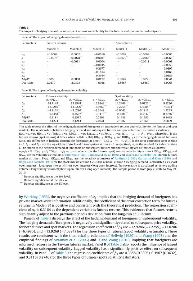
Table 3 reports the effect of the hedging demand of foreigners on subsequent returns and volatilityfor futures and spot markets.14 Panel A of Table 3 illustrates the impact of hedging demand of foreign-ers on subsequent returns. The hedging demand of foreigners has a significantly negative impact onsubsequent returns for futures and spot markets. The regression coefficients of ˛1 in Models (1), (2),and (3) are −0.0078, −0.0078, and −0.0081 for futures returns, and −0.0070, −0.0068, and −0.0063for spot returns, respectively. These results are inconsistent with hedging pressure effects. Never-theless, the results are consistent with the findings of de Roon et al. (2000) that hedging demand isnegatively related to subsequent returns for S&P 500 index futures, while the negative relationshipbetween hedging demand and subsequent returns in de Roon et al. (2000) is insignificant. As suggested

14 Before examining the effect of the hedging demand of institutional traders on subsequent returns and volatility for futuresand spot markets, this paper first tests for the stationarity of the time series of each variable in Tables 1 and 2. Using AugmentedDickey–Fuller (ADF) tests suggested by Dickey and Fuller (1979), the series of each variable appears to be stationary becausethe hypothesis of a unit root is rejected significantly with a p-value of 10% or lower.


Table 3The impact of hedging demand on subsequent returns and volatility for the futures and spot markets—foreigners.

Panel A: The impact of hedging demand on returns

Parameters Futures returns Spot returns

Model (1) Model (2) Model (3) Model (1) Model (2) Model (3)

˛0 −0.0009 0.0002 −0.0010 −0.0008 −0.0004 −0.0005˛1 −0.0078** −0.0078*** −0.0081** −0.0070** −0.0068** −0.0063**

˛2 – −0.0031 0.0004 – −0.0011 −0.0008˛3 – – -−0.0035 – – −0.0050˛4 – – 0.2677 – – 0.0397˛5 – – −0.1814 – – 0.0169˛6 – – 0.3164* – – −0.0389Adj-R2 0.0056 0.0050 0.0172 0.0062 0.0050 0.0041DW-stats 2.0270 2.0323 1.9988 1.8667 1.8689 1.9965

Panel B: The impact of hedging demand on volatility

Parameters Futures volatility Spot volatility�t = PKFM,t �t = GKFM,t �t = RSFM,t �t = PKSM,t �t = GKSM,t �t = RSSM,t

ˇ0 14.7149*** 13.8948*** 13.8848*** 11.2408 *** 9.6126*** 9.8286***

ˇ1 −12.9286*** −13.0206*** −13.9269*** −7.2255*** −6.4985*** −7.0324***

ˇ2 −4.9161** −3.6280* −2.2649 −2.0043 −0.1911 1.9245ˇ3 0.3358*** 0.3507*** 0.3116*** 0.3306*** 0.3632*** 0.2746***

Adj-R2 0.2181 0.2517 0.2295 0.1636 0.1982 0.1445DW-stats 2.1273 2.1213 2.0941 2.1302 2.1368 2.0899

This table reports the effect of the hedging demand of foreigners on subsequent returns and volatility for the futures and spotmarkets. The relationships between hedging demand and subsequent futures and spot returns are estimated as follows:Reti,t = ˛0 + ˛1 HDF,t − 1 + ˛2 TORF,t − 1 + ˛3 DHDF,t − 1 + ˛4 RetSM,t − 1 + ˛5 RetFM,t − 1 + ˛6 (St − 1 − �0 − �1 Ft − 1) + ei,t , where Reti,t is thefutures returns (spot returns) at time t when i = FM (i = SM). HDF,t − 1, TORF,t − 1, and DHDF,t − 1 are the hedging demand, turnoverratio, and difference in hedging demand for foreigners at time t − 1. (St−1 − �0 − �1 Ft−1) is the error correction term at timet − 1. St−1 and Ft−1 are the logarithms of stock and futures prices at time t − 1, respectively. ei,t is the residual for index i at timet. The effects of the hedging demand of foreigners on subsequent futures and spot volatility are estimated as follows:�t = ˇ0 + ˇ1 HDF,t − 1 + ˇ2 TORF,t − 1 + ˇ3 �t − 1 + εt , where �t is the futures (spot) annualized volatility at time t. PKFM,t , GKFM,t , andRSFM,t are the volatility estimators of Parkinson (1980), Garman and Klass (1980), and Rogers and Satchell (1991) for the futuresmarket at time t. PKSM,t , GKSM,t , and RSSM,t are the volatility estimators of Parkinson (1980), Garman and Klass (1980), andRogers and Satchell (1991) for the stock market at time t. εt is the residual at time t. Hedging demand is calculated as: (shortopen interest − long open interest)/(short open interest + long open interest). Turnover ratio is calculated as: (short tradingvolume + long trading volume)/(short open interest + long open interest). The sample period is from July 2, 2007 to May 21,2010.



by Working (1953), the negative coefficient of ˛1 implies that the hedging demand of foreigners hasprivate market-wide information. Additionally, the coefficient of the error correction term for futuresreturns in Model (3) is positive and consistent with the theoretical prediction. The regression coeffi-cient of ˛6 is 0.3164 as the dependent variable is futures returns. This evidences that futures returnssignificantly adjust to the previous period’s deviation from the long-run equilibrium.

Panel B of Table 3 displays the effect of the hedging demand of foreigners on subsequent volatility.The hedging demand of foreigners is negatively and significantly related to subsequent price volatility,for both futures and spot markets. The regression coefficients of ˇ1 are −12.9286 (−7.2255), −13.0206(−6.4985), and −13.9269 (−7.0324) for the three types of futures (spot) volatility estimators. Theseresults are consistent with the theoretical predictions of Hellwig (1980) and Wang (1993) and theempirical findings of Avramov et al. (2006) and Li and Wang (2010), implying that foreigners areinformed hedgers in the Taiwan futures market. Panel B of Table 3 also reports the influence of laggedvolatility on subsequent volatility. Lagged volatility has a significantly positive effect on subsequentvolatility. In Panel B of Table 3, the regression coefficients of ˇ3 are 0.3358 (0.3306), 0.3507 (0.3632),and 0.3116 (0.2746) for the three types of futures (spot) volatility estimators.


Table 4The impact of hedging demand on subsequent returns and volatility for the futures and spot markets—proprietary traders.




˛0 −0.0003 0.0006 −0.0027 −0.0003 −0.0026 −0.0027*

˛1 −0.0018 −0.0017 −0.0030 −0.0024 −0.0028 −0.0020˛2 – −0.0026 0.0009 – 0.0008 0.0009*

˛3 – – 0.0034 – – 0.0031˛4 – – 0.2606 – – 0.0423˛5 – – −0.1572 – – 0.0355˛6 – – 0.3648** – – 0.0117Adj-R2 −0.0005 −0.0013 0.0139 0.0009 0.0028 0.0022DW-stats 2.0268 2.0303 2.0030 1.8772 1.8744 2.0036


Parameters Futures volatility Spot volatility

�t = PKFM,t �t = GKFM,t �t = RSFM,t �t = PKSM,t �t = GKSM,t �t = RSSM,t

ˇ0 16.2411*** 15.2130*** 15.0754*** 12.8774*** 11.2020*** 11.2239***

ˇ1 7.5577*** 6.7062*** 6.7007*** 5.9784*** 4.9357*** 4.9967***

ˇ2 −1.1688*** −1.0858*** −0.8291** −0.5769** −0.4496** −0.0792ˇ3 0.3776*** 0.4135*** 0.3737*** 0.3146*** 0.3639*** 0.2714***

Adj-R2 0.2141 0.2387 0.2068 0.1835 0.2127 0.1495DW-stats 2.1298 2.1400 2.1210 2.0986 2.1099 2.0780

This table reports the effect of the hedging demand of proprietary traders on subsequent returns and volatility for the futures andspot markets. The relationships between hedging demand and subsequent futures and spot returns are estimated as follows:Reti,t = ˛0 + ˛1 HDP,t − 1 + ˛2 TORP,t − 1 + ˛3 DHDP,t − 1 + ˛4 RetSM,t − 1 + ˛5 RetFM,t − 1 + ˛6 (St − 1 − �0 − �1 Ft − 1) + ei,t , where Reti,t is thefutures returns (spot returns) at time t when i = FM (i = SM). HDP,t − 1, TORP,t − 1, and DHDP,t − 1 are the hedging demand, turnoverratio, and difference in hedging demand for proprietary traders at time t − 1. (St−1 − �0 − �1 Ft−1) is the error correction termat time t − 1. St−1 and Ft−1 are the logarithms of stock and futures prices at time t − 1, respectively. ei,t is the residual for index iat time t. The effects of the hedging demand of proprietary traders on subsequent futures and spot volatility are estimated asfollows:�t = ˇ0 + ˇ1 HDP,t − 1 + ˇ2 TORP,t − 1 + ˇ3 �t − 1 + εt , where �t is the futures (spot) annualized volatility at time t. PKFM,t , GKFM,t , andRSFM,t are the volatility estimators of Parkinson (1980), Garman and Klass (1980), and Rogers and Satchell (1991) for the futuresmarket at time t. PKSM,t , GKSM,t , and RSSM,t are the volatility estimators of Parkinson (1980), Garman and Klass (1980), andRogers and Satchell (1991) for the stock market at time t. εt is the residual at time t. Hedging demand is calculated as: (shortopen interest − long open interest)/(short open interest + long open interest). Turnover ratio is calculated as: (short tradingvolume + long trading volume)/(short open interest + long open interest). The sample period is from July 2, 2007 to May 21,2010.


*** Denote significance at the 1% level.

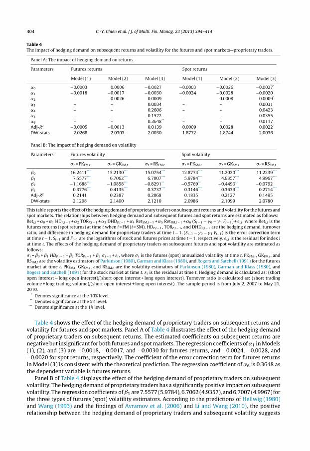
Table 4 shows the effect of the hedging demand of proprietary traders on subsequent returns andvolatility for futures and spot markets. Panel A of Table 4 illustrates the effect of the hedging demandof proprietary traders on subsequent returns. The estimated coefficients on subsequent returns arenegative but insignificant for both futures and spot markets. The regression coefficients of ˛1 in Models(1), (2), and (3) are −0.0018, −0.0017, and −0.0030 for futures returns, and −0.0024, −0.0028, and−0.0020 for spot returns, respectively. The coefficient of the error correction term for futures returnsin Model (3) is consistent with the theoretical prediction. The regression coefficient of ˛6 is 0.3648 asthe dependent variable is futures returns.

Panel B of Table 4 displays the effect of the hedging demand of proprietary traders on subsequentvolatility. The hedging demand of proprietary traders has a significantly positive impact on subsequentvolatility. The regression coefficients of ˇ1 are 7.5577 (5.9784), 6.7062 (4.9357), and 6.7007 (4.9967) forthe three types of futures (spot) volatility estimators. According to the predictions of Hellwig (1980)and Wang (1993) and the findings of Avramov et al. (2006) and Li and Wang (2010), the positiverelationship between the hedging demand of proprietary traders and subsequent volatility suggests


Table 5The impact of hedging demand on subsequent returns and volatility for the futures and spot markets—mutual funds.




˛0 −0.0003 0.0008 0.0001 −0.0002 −0.0002 −0.0003˛1 0.0000 −0.0003 −0.0002 −0.0002 −0.0002 0.0001˛2 – −0.0040 −0.0013 – −0.0001 0.0000˛3 – – −0.0178 – – −0.0122˛4 – – 0.2449 – – 0.0253˛5 – – −0.1732 – – 0.0257˛6 – – 0.2995* – – −0.0362Adj-R2 −0.0014 −0.0015 0.0122 −0.0014 −0.0028 −0.0011DW-stats 2.0129 2.0171 1.9955 1.8536 1.8538 1.9950




ˇ0 11.3701*** 10.6261*** 10.5744*** 9.5605*** 8.3903*** 8.7399***

ˇ1 6.0071*** 5.2470*** 5.1782*** 4.2751*** 3.6377*** 3.8482***

ˇ2 −1.8239 −0.6809 0.6020 −1.1101 −0.1880 1.3134ˇ3 0.3414*** 0.3785*** 0.3544*** 0.3126*** 0.3567*** 0.2784***

Adj-R2 0.1992 0.2215 0.1933 0.1672 0.1988 0.1409DW-stats 2.1510 2.1664 2.1427 2.1194 2.1350 2.0963

This table reports the effect of the hedging demand of mutual funds on subsequent returns and volatility for the futures andspot markets. The relationships between hedging demand and subsequent futures and spot returns are estimated as follows:Reti,t = ˛0 + ˛1 HDM,t − 1 + ˛2 TORM,t − 1 + ˛3 DHDM,t − 1 + ˛4 RetSM,t − 1 + ˛5 RetFM,t − 1 + ˛6 (St − 1 − �0 − �1 Ft − 1) + ei,t , where Reti,t is thefutures returns (spot returns) at time t when i = FM (i = SM). HDM,t − 1, TORM,t − 1, and DHDM,t − 1 are the hedging demand, turnoverratio, and difference in hedging demand for mutual funds at time t − 1. (St−1 − �0 − �1 Ft−1) is the error correction term at timet − 1. St − 1 and Ft−1 are the logarithms of stock and futures prices at time t − 1, respectively. ei,t is the residual for index i at timet. The effects of the hedging demand of mutual funds on subsequent futures and spot volatility are estimated as follows:�t = ˇ0 + ˇ1 HDM,t − 1 + ˇ2 TORM,t − 1 + ˇ3 �t − 1 + εt , where �t is the futures (spot) annualized volatility at time t. PKFM,t , GKFM,t ,and RSFM,t are the volatility estimators of Parkinson (1980), Garman and Klass (1980), and Rogers and Satchell (1991) for thefutures market at time t. PKSM,t , GKSM,t , and RSSM,t are the volatility estimators of Parkinson (1980), Garman and Klass (1980),and Rogers and Satchell (1991) for the stock market at time t. εt is the residual at time t. Hedging demand is calculated as: (shortopen interest − long open interest)/(short open interest + long open interest). Turnover ratio is calculated as: (short tradingvolume + long trading volume)/(short open interest + long open interest). The sample period is from July 2, 2007 to May 21,2010.



that proprietary traders are not informed hedgers, as volatility increases with liquidity (or uninformed)trading. Panel B of Table 4 also reports the influence of lagged volatility on subsequent volatility. Laggedvolatility has a significantly positive effect on subsequent volatility. The regression coefficients of ˇ3in Panel B of Table 4 are 0.3776 (0.3146), 0.4135 (0.3639), and 0.3737 (0.2714) for the three types offutures (spot) volatility estimators.

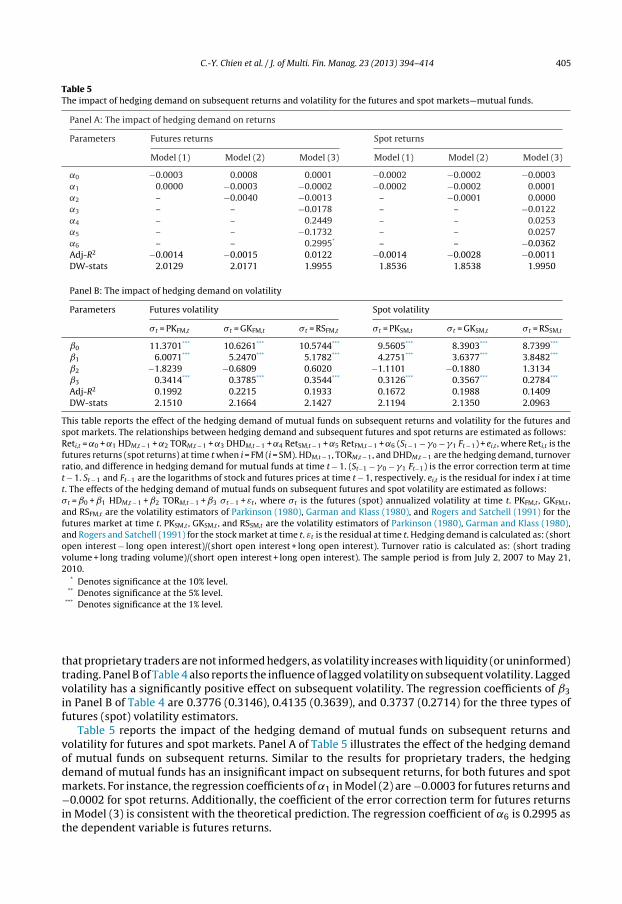
Table 5 reports the impact of the hedging demand of mutual funds on subsequent returns andvolatility for futures and spot markets. Panel A of Table 5 illustrates the effect of the hedging demandof mutual funds on subsequent returns. Similar to the results for proprietary traders, the hedgingdemand of mutual funds has an insignificant impact on subsequent returns, for both futures and spotmarkets. For instance, the regression coefficients of ˛1 in Model (2) are −0.0003 for futures returns and−0.0002 for spot returns. Additionally, the coefficient of the error correction term for futures returnsin Model (3) is consistent with the theoretical prediction. The regression coefficient of ˛6 is 0.2995 asthe dependent variable is futures returns.


Panel B of Table 5 displays the effect of the hedging demand of mutual funds on subsequent volatil-ity. The hedging demand of mutual funds has a significantly positive impact on subsequent volatility.The regression coefficients of ˇ1 are 6.0071, 5.2470 and 5.1782 for the three types of futures volatilityestimators, and 4.2751, 3.6377 and 3.8482 for the three types of spot volatility estimators. Similar tothe results of Table 4, the positive relationship between the hedging demand of mutual funds andsubsequent volatility implies that mutual funds are not informed hedgers, as volatility increases withliquidity (or uninformed) trading. Panel B of Table 5 also reports the influence of lagged volatility onsubsequent volatility. Lagged volatility has a significantly positive effect on subsequent volatility. Theregression coefficients of ˇ3 in Panel B of Table 5 are 0.3414 (0.3126), 0.3785 (0.3567), and 0.3544(0.2784) for the three types of futures (spot) volatility estimators.

6.3. Impact of hedging demand of all types of institutional trader

The hedging demand of each type of institutional trader may interact with the hedging demand ofothers. To control this possible interaction, this paper includes the hedging demand of various types ofinstitutional trader in the regression model. Table 6 reports the effect of the hedging demand of insti-tutional traders on subsequent returns and volatility for futures and spot markets. Panel A of Table 6shows the effects of hedging demands of institutional traders on subsequent returns. Consistent withthe results presented in Tables 3–5, the hedging demand of foreigners is significantly and negativelyrelated to subsequent returns. The coefficient estimate of the hedging demand of foreigners is nega-tive, at a value of −0.0096 (−0.0070), for futures (spot) returns. Moreover, the impacts of the hedgingdemands of proprietary traders and mutual funds on subsequent returns are insignificant. Panel B ofTable 6 reports the effect of the hedging demand of institutional traders on subsequent volatility. Thehedging demand of foreigners has a significantly negative effect on subsequent volatility. The coeffi-cient of the hedging demand of foreigners is significantly negative, at values of −10.8405 (−5.1266),−11.4592 (−4.8685), and −10.2027 (−4.9711) for the three types of futures (spot) volatility estima-tors. In contrast, the hedging demands of proprietary traders and mutual funds have a significant andpositive impact on subsequent volatility. As the coefficients of foreigners are negative for subsequentfutures (spot) returns and volatility, this paper suggests that foreigners are informed hedgers in theTaiwan futures market.

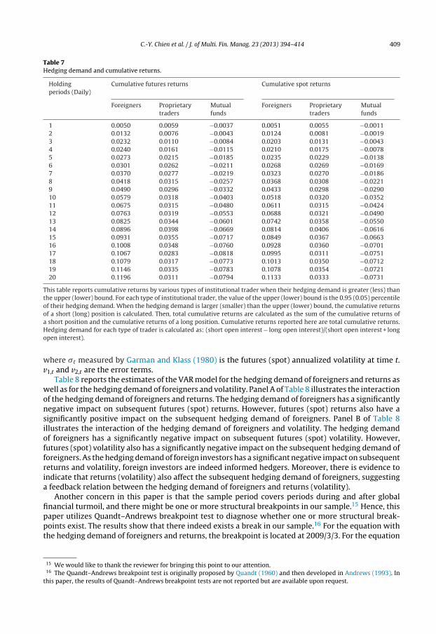
In addition, this study also examines the relationship between trading rules based on the extremehedging demand of institutional traders and trading performance. If the trading rule based on thehedging demand of institutional traders is positively correlated with trading performance, investorscan profit from hedging demand information. Wang (2004) indicates that extreme sentiment by tradertype is more correlated with future market movements than moderate sentiment. As this paper arguesthat foreigners are informed hedgers, we expect that a strategy conditional on the large positive(negative) hedging demand of foreigners should be more profitable than those conditional on thelarge positive (negative) hedging demand of the other two institutional traders. To test this argument,this paper examines the profitability of the following trading rule. For each type of institutional trader,the value of the upper (lower) bound is the 0.95 (0.05) percentile of their hedging demand. When thehedging demand is larger (smaller) than upper (lower) bound, the cumulative returns of a short (long)position are calculated. Then, total cumulative returns are calculated as the sum of the cumulativereturns of a short position and the cumulative returns of a long position.

Figs. 2 and 3 present the relationship between the extreme hedging demand of institutionalinvestors and total cumulative returns for futures and spot markets over the holding periods. As theresults shown in Figs. 2 and 3 are similar, our interpretations focus on the results shown in Fig. 2.In Fig. 2, the total cumulative futures returns regarding the extreme hedging demand of foreignersare positive and are largest over the holding period. Total cumulative returns regarding the extremehedging demand of mutual funds are negative and smallest during the holding period. Table 7 reportstotal cumulative returns by various types of institutional trader when their hedging demand is greater(less) than the upper (lower) bound. Consistent with conjecture, Table 7 shows that a strategy con-ditional on a large positive (negative) hedging demand of foreigners is more profitable than thoseconditional on a large positive (negative) hedging demand of the other two types of institutionaltrader. As the holding period increases, the total cumulative futures (spot) returns based on the upper


Table 6The impact of hedging demand on subsequent returns and volatility for the futures and spot markets—all institutional traders.



˛0 −0.0021 −0.0022˛1 −0.0096*** −0.0070**

˛2 −0.0042 −0.0030˛3 −0.0008 −0.0001˛4 0.0002 −0.0040˛5 0.0007 0.0009*

˛6 −0.0020 0.0014˛7 0.2154 0.0053˛8 −0.1468 0.0421˛9 0.3729** 0.0065Adj-R2 0.0191 0.0059DW-stats 2.0022 2.0030




ˇ0 15.2782*** 14.6323*** 14.6122*** 11.5711*** 10.1713*** 11.3814***

ˇ1 −10.8405*** −11.4592*** −10.2027*** −5.1266*** −4.8685*** −4.9711***

ˇ2 6.2117*** 5.8100*** 6.1570*** 4.9968*** 4.6216*** 5.5065***

ˇ3 3.2362*** 2.9995*** 3.7408*** 2.6728*** 2.9078*** 3.1922***

ˇ4 −4.1103 −3.7225 −4.3811 −0.2741 1.4338 −0.3984ˇ5 −0.5534 −0.4413 0.5157 −0.2261 0.0653 −0.0089ˇ6 2.4607 3.8434 3.6543 −0.1069 −0.0068 0.2744ˇ7 0.2682*** 0.2676*** 0.2830*** 0.2408*** 0.2021*** 0.2163***

Adj-R2 0.2635 0.2899 0.2652 0.2118 0.2236 0.2030DW-stats 2.0638 2.0199 1.9533 2.0619 1.9261 1.8544

This table reports the effect of the hedging demand of all institutional traders on subsequent returns and volatility for thefutures and spot markets. The relationships between hedging demand and subsequent futures and spot returns are estimatedas follows:Reti,t = ˛0 + ˛1 HDF,t − 1 + ˛2 HDP,t − 1 + ˛3 HDM,t − 1 + ˛4 TORF,t − 1 + ˛5 TORP,t − 1 + ˛6 TORM,t − 1 + ˛7 RetSM,t − 1 + ˛8 RetFM,t − 1 + ˛9

(St − 1−�0−�1 Ft − 1) + ei,t , where Reti,t is the futures returns (spot returns) at time t when i = FM (i = SM). HDF,t − 1, HDP,t − 1, andHDM,t − 1 are the hedging demand for foreigners, proprietary traders, and mutual funds at time t − 1. TORF,t − 1, TORP,t − 1, andTORM,t − 1 are the turnover ratios for foreigners, proprietary traders, and mutual funds at time t − 1. (St−1 − �0 − �1 Ft−1) is theerror correction term at time t − 1. St−1 and Ft−1 are the logarithms of stock and futures prices at time t − 1, respectively. ei,t

is the residual for index i at time t. The effects of the hedging demand of institutional traders on subsequent futures and spotvolatility are estimated as follows:�t = ˇ0 + ˇ1 HDF,t − 1 + ˇ2 HDP,t − 1 + ˇ3 HDM,t − 1 + ˇ4 TORF,t − 1 + ˇ5 TORP,t − 1 + ˇ6 TORM,t − 1 + ˇ7 �t − 1 + εt , where �t is the futures(spot) annualized volatility at time t. PKFM,t , GKFM,t , and RSFM,t are the volatility estimators of Parkinson (1980), Garman andKlass (1980), and Rogers and Satchell (1991) for the futures market at time t. PKSM,t , GKSM,t , and RSSM,t are the volatility esti-mators of Parkinson (1980), Garman and Klass (1980), and Rogers and Satchell (1991) for the stock market at time t. εt is theresidual at time t. Hedging demand for each type of trader is calculated as: (short open interest−long open interest)/(shortopen interest + long open interest). Turnover ratio for each type of trader is calculated as: (short trading volume + long tradingvolume)/(short open interest + long open interest). The sample period is from July 2, 2007 to May 21, 2010.



and lower bounds of the hedging demand of foreigners increases from 0.0050 (0.0051) to 0.1196(0.1133). However, the cumulative returns based on the upper and lower bounds of the hedgingdemand of mutual funds decreases from −0.0037 (−0.0011) to −0.0794 (−0.0731), and the cumulativereturns based on the upper and lower bounds of the hedging demand of proprietary traders slightlyincrease from 0.0059 (0.0055) to 0.0311 (0.0333). Again, these findings provide evidence that thehedging demand of foreign investors contains more information than that of proprietary traders andmutual funds.


Holding Periods (Daily)

Cu

mu

lati

ve F

utu

res

Ret

urn

s

1 2 3 4 5 6 7 8 9 10 11 12 13 14 15 16 17 18 19 20-0.100

-0.075

-0.050

-0.025

-0.000

0.025

0.050

0.075

0.100

0.125

Foreigners

Proprietary Traders

Mutual Funds

Fig. 2. Hedging demand and cumulative futures returns.

Holding Periods (Daily)

Cu

mu

lati

ve S

po

t R

etu

rns

1 2 3 4 5 6 7 8 9 10 11 12 13 14 15 16 17 18 19 20-0.100

-0.075

-0.050

-0.025

-0.000

0.025

0.050

0.075

0.100

0.125

Foreigners

Proprietary Traders

Mutual Funds

Fig. 3. Hedging demand and cumulative spot returns.

6.4. Robustness tests

In this section, we check the robustness regarding whether foreign investors are informed hedgers.First, this paper considers a question of possible endogeneity. Second, this paper considers the impactof global financial turmoil.

In order to control for possible endogeneity, we run vector autoregressive (VAR) models for thehedging demand of foreigners and returns as well as for the hedging demand of foreigners and volatil-ity. A VAR model between the hedging demand of foreigners and returns can be expressed as follows:

Reti,t = a0 + a1Reti,t−1 + a2HDF,t−1 + u1,t, (8)

HDF,t = b0 + b1Reti,t−1 + b2HDF,t−1 + u2,t, (9)

where Reti,t is the futures returns (spot returns) at time t when i = FM (i = SM). HDF,t is the hedgingdemand for foreigners at time t. u1,t and u2,t are the error terms.

In addition, a VAR model between the hedging demand of foreigners and volatility can be expressedas follows:

�t = c0 + c1�t−1 + c2 HDF,t−1 + v1,t, (10)

HDF,t = d0 + d1�t−1 + d2HDF,t−1 + v2,t, (11)


Table 7Hedging demand and cumulative returns.

Holdingperiods (Daily)

Cumulative futures returns Cumulative spot returns

Foreigners Proprietarytraders

Mutualfunds

Foreigners Proprietarytraders

Mutualfunds

1 0.0050 0.0059 −0.0037 0.0051 0.0055 −0.00112 0.0132 0.0076 −0.0043 0.0124 0.0081 −0.00193 0.0232 0.0110 −0.0084 0.0203 0.0131 −0.00434 0.0240 0.0161 −0.0115 0.0210 0.0175 −0.00785 0.0273 0.0215 −0.0185 0.0235 0.0229 −0.01386 0.0301 0.0262 −0.0211 0.0268 0.0269 −0.01697 0.0370 0.0277 −0.0219 0.0323 0.0270 −0.01868 0.0418 0.0315 −0.0257 0.0368 0.0308 −0.02219 0.0490 0.0296 −0.0332 0.0433 0.0298 −0.029010 0.0579 0.0318 −0.0403 0.0518 0.0320 −0.035211 0.0675 0.0315 −0.0480 0.0611 0.0315 −0.042412 0.0763 0.0319 −0.0553 0.0688 0.0321 −0.049013 0.0825 0.0344 −0.0601 0.0742 0.0358 −0.055014 0.0896 0.0398 −0.0669 0.0814 0.0406 −0.061615 0.0931 0.0355 −0.0717 0.0849 0.0367 −0.066316 0.1008 0.0348 −0.0760 0.0928 0.0360 −0.070117 0.1067 0.0283 −0.0818 0.0995 0.0311 −0.075118 0.1079 0.0317 −0.0773 0.1013 0.0350 −0.071219 0.1146 0.0335 −0.0783 0.1078 0.0354 −0.072120 0.1196 0.0311 −0.0794 0.1133 0.0333 −0.0731

This table reports cumulative returns by various types of institutional trader when their hedging demand is greater (less) thanthe upper (lower) bound. For each type of institutional trader, the value of the upper (lower) bound is the 0.95 (0.05) percentileof their hedging demand. When the hedging demand is larger (smaller) than the upper (lower) bound, the cumulative returnsof a short (long) position is calculated. Then, total cumulative returns are calculated as the sum of the cumulative returns ofa short position and the cumulative returns of a long position. Cumulative returns reported here are total cumulative returns.Hedging demand for each type of trader is calculated as: (short open interest − long open interest)/(short open interest + longopen interest).

where �t measured by Garman and Klass (1980) is the futures (spot) annualized volatility at time t.v1,t and v2,t are the error terms.

Table 8 reports the estimates of the VAR model for the hedging demand of foreigners and returns aswell as for the hedging demand of foreigners and volatility. Panel A of Table 8 illustrates the interactionof the hedging demand of foreigners and returns. The hedging demand of foreigners has a significantlynegative impact on subsequent futures (spot) returns. However, futures (spot) returns also have asignificantly positive impact on the subsequent hedging demand of foreigners. Panel B of Table 8illustrates the interaction of the hedging demand of foreigners and volatility. The hedging demandof foreigners has a significantly negative impact on subsequent futures (spot) volatility. However,futures (spot) volatility also has a significantly negative impact on the subsequent hedging demand offoreigners. As the hedging demand of foreign investors has a significant negative impact on subsequentreturns and volatility, foreign investors are indeed informed hedgers. Moreover, there is evidence toindicate that returns (volatility) also affect the subsequent hedging demand of foreigners, suggestinga feedback relation between the hedging demand of foreigners and returns (volatility).

Another concern in this paper is that the sample period covers periods during and after globalfinancial turmoil, and there might be one or more structural breakpoints in our sample.15 Hence, thispaper utilizes Quandt–Andrews breakpoint test to diagnose whether one or more structural break-points exist. The results show that there indeed exists a break in our sample.16 For the equation withthe hedging demand of foreigners and returns, the breakpoint is located at 2009/3/3. For the equation

15 We would like to thank the reviewer for bringing this point to our attention.16 The Quandt–Andrews breakpoint test is originally proposed by Quandt (1960) and then developed in Andrews (1993). In

this paper, the results of Quandt–Andrews breakpoint tests are not reported but are available upon request.

410C.-Y.

Chien et

al. /

J. of

Multi.

Fin. M

anag. 23 (2013) 394– 414

Table 8Estimates of vector autoregressive (VAR) models for hedging demand and returns as well as for hedging demand and volatility—foreigners.

Panel A: VAR models for hedging demand and returns

Futures Returns Hedging demand Spot Returns Hedging demand

Coefficient Coefficient Coefficient Coefficient

a0 −0.0009 (−1.0947) b0 −0.0023 (−1.1296) a0 −0.0008 (−1.1103) b0 −0.0023 (−1.1420)a1 −0.0147 (−0.3927) b1 0.2515*** (2.7276) a1 0.0650* (1.7392) b1 0.2504** (2.2667)a2 −0.0080** (−2.2821) b2 0.9744*** (113.2905) a2 −0.0064** (−2.2014) b2 0.9740*** (113.0788)Adj-R2 0.0045 Adj-R2 0.9473 Adj-R2 0.0091 Adj-R2 0.9471

Panel B: VAR models for hedging demand and volatility

Futures Volatility Hedging demand Spot Volatility Hedging demand


c0 12.9230*** (16.5058) d0 0.0071* (1.7177) c0 9.5640*** (16.1675) d0 0.0072* (1.6701)c1 0.3371*** (9.6565) d1 −0.0005*** (−2.6536) c1 0.3621*** (10.4325) d1 −0.0006** (−2.5515)c2 −13.1973*** (−7.5798) d2 0.9631*** (104.2321) c2 −6.5050*** (−5.3071) d2 0.9662*** (108.5685)Adj-R2 0.2490 Adj-R2 0.9473 Adj-R2 0.1993 Adj-R2 0.9473

This table reports the estimates of vector autoregressive (VAR) models for the hedging demand of foreigners and returns as well as for the hedging demand of foreigners and volatility. AVAR model between hedging demand of foreigners and returns could be expressed as follows:Reti,t = a0 + a1Reti,t − 1 + a2HDF,t − 1 + u1,t , HDF,t = b0 + b1Reti,t − 1 + b2HDF,t − 1 + u2,t , where Reti,t is the futures returns (spot returns) at time t when i = FM (i = SM). HDF,t is the hedging demandfor foreigners at time t. u1,t and u2,t are the error terms.In addition, a VAR model between the hedging demand of foreigners and volatility could be expressed as follows:�t = c0 + c1�t − 1 + c2HDF,t − 1 + v1,t , HDF,t = d0 + d1�t − 1 + d2HDF,t − 1 + v2,t , where �t measured by Garman and Klass (1980) is the futures (spot) annualized volatility at time t. v1,t and v2,t are theerror terms. The sample period is from July 2, 2007 to May 21, 2010.



C.-Y. Chien

et al.

/ J.

of M

ulti. Fin.

Manag.

23 (2013) 394– 414411

Table 9Estimates of vector autoregressive (VAR) models during and after the global financial turmoil—foreigners.

Panel A: VAR models for hedging demand and returns—during the global financial turmoil

Futures returns Hedging demand Spot returns Hedging demand


a0 −0.0021* (−1.6640) b0 −0.0030 (−1.0892) a0 −0.0019* (−1.8021) b0 −0.0029 (−1.0852)a1 −0.0579 (−1.1666) b1 0.1777* (1.6714) a1 0.0266 (0.5351) b1 0.1911 (1.4579)a2 −0.0029 (−0.5941) b2 0.9814*** (95.4194) a2 −0.0021 (−0.5268) b2 0.9813*** (95.3445)Adj-R2 −0.0008 Adj-R2 0.9570 Adj-R2 −0.0035 Adj-R2 0.9569Panel B: VAR models for hedging demand and volatility—during the global financial turmoilc0 14.1154*** (12.0373) d0 0.0070 (1.1462) c0 10.9278*** (12.3217) d0 0.0056 (0.8957)c1 0.3489*** (7.2447) d1 −0.0004* (−1.7230) c1 0.3320*** (6.8326) d1 −0.0005 (−1.4162)c2 −18.3260*** (−6.8452) d2 0.9603*** (69.2403) c2 −9.7685*** (−5.2910) d2 0.9651*** (73.8641)Adj-R2 0.3378 Adj-R2 0.9449 Adj-R2 0.2358 Adj-R2 0.9448Panel C: VAR models for hedging demand and returns—after the global financial turmoila0 0.0003 (0.2799) b0 −0.0021 (−0.6643) a0 0.0003 (0.3773) b0 −0.0021 (−0.6663)a1 0.0675 (1.1976) b1 0.4332** (2.2555) a1 0.1044* (1.8449) b1 0.3327 (1.5620)a2 −0.0198*** (−4.1934) b2 0.9599*** (59.7273) a2 −0.0171*** (−3.9980) b2 0.9572*** (59.3464)Adj-R2 0.0632 Adj-R2 0.9237 Adj-R2 0.0674 Adj-R2 0.9231Panel D: VAR models for hedging demand and volatility—after the global financial turmoilc0 14.8724*** (14.0215) d0 0.0104* (1.6566) c0 9.3615*** (11.6634) d0 0.0109* (1.7458)c1 0.1445*** (2.7315) d1 −0.0007** (−2.3742) c1 0.3121*** (6.0830) d1 −0.0010** (−2.4794)c2 −11.7854*** (−5.3531) d2 0.9633*** (74.2679) c2 −4.9793*** (−3.0627) d2 0.9661*** (76.5736)Adj-R2 0.1226 Adj-R2 0.9478 Adj-R2 0.1380 Adj-R2 0.9479

This table reports, during and after the global financial turmoil, the estimates of vector autoregressive (VAR) models for the hedging demand of foreigners and returns as well as for thehedging demand of foreigners and volatility. The Quandt–Andrews Breakpoint test is utilized to diagnose structural breaks during and after the global financial turmoil. A VAR modelbetween the hedging demand of foreigners and returns could be expressed as follows:Reti,t = a0 + a1Reti,t − 1 + a2HDF,t − 1 + u1,t , HDF,t = b0 + b1Reti,t − 1 + b2HDF,t − 1 + u2,t , where Reti,t is the futures returns (spot returns) at time t when i = FM (i = SM). HDF,t is the hedging demandfor foreigners at time t. u1,t and u2,t are the error terms.In addition, a VAR model between the hedging demand of foreigners and volatility could be expressed as follows:�t = c0 + c1�t − 1 + c2HDF,t − 1 + v1,t ,HDF,t = d0 + d1�t − 1 + d2HDF,t − 1 + v2,t , where �t measured by Garman and Klass (1980) is the futures (spot) annualized volatility at time t. v1,t and v2,t are the error terms. The sample periodis from July 2, 2007 to May 21, 2010.




with the hedging demand of foreigners and volatility, the breakpoint is located at 2009/1/6. As notedby Ivashina and Scharfstein (2010), the financial turmoil period ends at December 2008. Thus, thestructural break helps to divide the sample period into the global financial turmoil subperiod and thepost global financial turmoil subperiod.

Then, we compare the results of the VAR models during and after the global financial turmoil.Table 9 presents the estimates of the VAR models for the hedging demand of foreigners and returns aswell as for the hedging demand of foreigners and volatility in the global financial turmoil subperiod andthe post global financial turmoil subperiod.17 Panel A of Table 9 presents the interaction of the hedgingdemand of foreigners and returns in the global financial turmoil subperiod. Panel B of Table 9 presentsthe interaction of the hedging demand of foreigners and volatility in the global financial turmoilsubperiod. The results indicate that, during global financial turmoil, the hedging demand of foreignersand returns do not have a strong relationship, but the hedging demand of foreigners has a significantlynegative impact on subsequent volatility. Moreover, Panel C of Table 9 presents the interaction of thehedging demand of foreigners and returns in the post global financial turmoil subperiod. Panel D ofTable 9 presents the interaction of the hedging demand of foreigners and volatility in the post globalfinancial turmoil subperiod. The results show that, after the global financial turmoil, the hedgingdemand of foreigners has a significantly negative impact on subsequent returns (volatility). Thus,relative to the global financial turmoil period, foreign investors are more informed after the globalfinancial turmoil.

7. Conclusions

This study uses data from the Taiwan futures market to examine how the hedging demand ofvarious types of institutional trader affects market returns and price volatility. Although previousstudies explore the institutional investor flows on stock and option markets, little research examinesthis issue on futures markets. This paper uses hedging demand as a proxy of investor flow to addressthis issue. As suggested by Working (1953), if hedgers are informed traders, their hedging demandwill be negatively associated with subsequent market returns. In addition, according to the theoreticalprediction of Hellwig (1980) and Wang (1993) and the empirical findings of Avramov et al. (2006) andLi and Wang (2010), if hedgers are informed traders, their hedging demand will be negatively relatedto subsequent price volatility. Taken together, hedging demand will be negatively associated withsubsequent returns as well as volatility if hedgers are informed traders.

On April 7, 2008, the TAIFEX published the daily trading activity of institutional investors. Thedata detail daily trading volume and open interests for foreign investors, proprietary traders, andmutual funds. The data used in this study include both bear and bull markets, from July 2, 2007 toMay 21, 2010. Empirical results indicate that foreigners are informed hedgers in the Taiwan futuresmarket, because the hedging demand of foreigners has a significantly negative impact on both sub-sequent returns and volatility. In contrast, proprietary traders and mutual funds are not informedhedgers because the relationship between hedging demand and subsequent returns is insignificant,and hedging demand has a significantly positive impact on subsequent volatility. In addition, trad-ing performance based on the extreme hedging demand of foreign investors is more profitable thanthat of proprietary traders and mutual funds. Furthermore, there is evidence to indicate that returns(volatility) also affect the subsequent hedging demand of foreign investors, suggesting a feedbackrelation. Finally, the hedging demand of foreign investors has a greater impact on subsequent returnsand volatility after global financial turmoil. Therefore, our findings have implications for academics interms of understanding the effects of the hedging demands of various types of institutional investorand for practitioners to develop trading strategies with regards to the hedging position of institutionalinvestors.

17 Testing for Granger causality (Granger, 1969) can be conducted within the context of a VAR model. As the results of theVAR models and Granger causality tests are very similar, for brevity, this paper only shows the results of the VAR models.


Acknowledgments

We would like to thank the editor, Professor Stephen Ferris, and an anonymous referee for help-ful comments and suggestions. All remaining errors are our own. Hsiu-Chuan Lee is grateful for thefinancial support from the National Science Council of Taiwan (NSC 100-2410-H-130-023).

References

Admati, A., Pfleiderer, P., 1988. A theory of intraday patterns: volume and price variability. Rev. Finan. Stud. 1, 3–40.Andrews, D., 1993. Tests for parameter instability and structural change with unknown change point. Econometrica 61,

821–856.Avramov, D., Chordia, T., Goyal, A., 2006. The impact of trades on daily volatility. Rev. Finan. Stud. 19, 1241–1277.Bae, K.H., Yamada, T., Ito, K., 2008. Interaction of investor trades and market volatility: evidence from Tokyo Stock Exchange.

Pac.-Basin Finan. J. 16, 370–388.Bailey, W., Cai, J., Cheung, Y.L., Wang, F., 2009. Stock returns, order imbalances, and commonality: evidence on individual,

institutional, and proprietary investors in China. J. Banking Finan. 33, 9–19.Baker, M., Stein, J.C., 2004. Market liquidity as a sentiment indicator. J. Finan. Markets 7, 271–299.Bessembinder, H., 1992. Systematic risk, hedging pressure, and risk premiums in futures markets. Rev. Finan. Stud. 5,

637–667.Bessembinder, H., Seguin, P.J., 1993. Price volatility, trading volume, and market depth: evidence from futures markets. J. Finan.

Quant. Anal. 28, 21–39.Boyer, B., Zheng, L., 2009. Investor flows and stock market returns. J. Empirical Finance 16, 87–100.Brennan, M.J., Cao, H., 1997. International portfolio investment flows. J. Finance 52, 1851–1880.Chan, K., Menkveld, A.J., Yang, Z., 2007. The informativeness of domestic and foreign investors’ stock trades: evidence from the

perfectly segmented Chinese market. J. Finan. Markets 10, 391–415.Chang, C.C., Hsieh, P.F., Lai, H.N., 2009. Do informed option investors predict stock returns? evidence from the Taiwan stock

exchange. J. Banking Finance 33, 757–764.Chang, E., Chou, R.Y., Nelling, E.F., 2000. Market volatility and the demand for hedging in stock index futures. J. Futures Markets

20, 105–125.Chang, E., Pinegar, M., Schachter, B., 1997. Interday variations in volume, variance, and participation of large speculators. J.

Banking Finance 21, 797–810.Chen, Z., Daigler, R.T., 2008. An examination of the complementary volume-volatility information theories. J. Futures Markets

28, 963–992.Chiao, C., Chen, S.H., Hu, J.M., 2010. Informational differences among institutional investors in an increasingly institutionalized

market. Japan World Economy 22, 118–129.Chiao, C., Wang, Z.M., Lai, H.L., 2009. Order submission behaviors and opening price behaviors: evidence from an emerging

market. Rev. Quant. Finance Acc. 33, 253–278.Choe, H., Kho, B.C., Stulz, R.M., 2005. Do domestic investors have an edge? the trading experience of foreign investors in Korea.

Rev. Finan. Stud. 18, 795–829.Chou, R.K., Wang, Y.Y., 2009. Strategic order splitting, order choice, and aggressiveness: evidence from Taiwan futures exchange.

J. Futures Markets 29, 1102–1129.de Roon, F., Nijman, T.E., Veld, C., 2000. Hedging pressure effects in futures markets. J. Finance 55, 1437–1456.Dickey, D.A., Fuller, W.A., 1979. Distribution of the estimators for autoregressive time series with a unit root. J. Am. Stat. Assoc.

74, 427–431.Dvorak, T., 2005. Do domestic investors have an information advantage? evidence from Indonesia. J. Finance 60, 817–839.Froot, K.A., O’Connell, P.G.J., Seasholes, M.S., 2001. The portfolio flows of international investors. J. Finan. Econ. 59, 151–193.Garman, M., Klass, M., 1980. On the estimation of security price volatilities from historical data. J. Bus. 53, 67–78.Granger, C., 1969. Investigate causal relations by econometric models and cross spectral methods. Econometrica 37,

424–438.Grinblatt, M., Keloharju, M., 2000. The investment behavior and performance of various investor types: a study of Finland’s

unique data set. J. Finan. Econ. 55, 43–67.Hellwig, M.F., 1980. On the aggregation of information in competitive markets. J. Econ. Theory 22, 477–498.Ivashina, V., Scharfstein, D., 2010. Bank lending during the financial crisis of 2008. J. Finan. Econ. 97, 319–338.Jacob, Vipul, J., 2008. Estimation and forecasting of stock volatility with range-based estimators. J. Futures Markets 28,

561–581.Li, W., Wang, S.S., 2010. Daily institutional trades and stock price volatility in a retail investor dominated emerging market. J.

Finan. Markets 13, 448–474.Luo, J.S., Li, C.A., 2008. Futures market sentiment and institutional investor behavior in the spot market: the emerging market

in Taiwan. Emerg. Markets Finance Trade 44, 70–86.Newey, W., West, K., 1987. A simple, positive semi-definite, heteroskedasticity and autocorrelation consistent covariance matrix.

Econometrica 55, 703–708.Pan, M.S., Liu, Y.A., Roth, H.J., 2003. Volatility and trading demands in stock index futures. J. Futures Markets 23, 399–414.Parkinson, M., 1980. The extreme value method for estimating the variance of the rate of return. J. Bus. 53, 61–65.Quandt, R., 1960. Tests of the hypothesis that a linear regression system obeys two separate regimes. J. Am. Stat. Assoc. 55,

324–330.Rogers, L.C.G., Satchell, S.E., 1991. Estimating variance from high, low and closing prices. Ann. Appl. Probab. 1, 504–512.Shalen, C.T., 1993. Volume, volatility, and the dispersion of beliefs. Rev. Finan. Stud. 6, 405–434.Vipul, Jacob, J., 2007. Forecasting performance of extreme-value volatility estimators. J. Futures Markets 27, 1085–1105.

http://refhub.elsevier.com/S1042-444X(13)00033-9/sbref0005








































































































































































































































































































































































































































































































































































































































































Wang, C., 2002. Information, trading demand, and futures price volatility. Finan. Rev. 37, 295–316.Wang, C., 2003. The behavior and performance of major types of futures traders. J. Futures Markets 23, 1–31.Wang, C., 2004. Futures trading activity and predictable foreign exchange market movements. J. Banking Finance 28,

1023–1041.Wang, J., 1993. A model of intertemporal asset prices under asymmetric information. Rev. Econ. Stud. 60, 249–282.Working, H., 1953. Futures trading and hedging. Am. Econ. Rev. 43, 314–343.










































































information, hedging demand, and institutional investors: evidence from the taiwan futures exchange

Documents